Abbas Edalat

Imperial College London

www.doc.ic.ac.uk/~ae

joint work with Marko Krznaric and Andre Lieutier

Domain-theoretic Solution of Differential EquationsDomain-theoretic Solution of Differential Equations

2

AimAim

• Develop data types for ordinary differential equations.

• Solve initial value problems up to any given precision:

= v(t,x) with v: R2 R continuous and Lipschitz in x

x(t0) = x0 with (t0,x0) R2

dt

dx

3

• Let IR={ [a,b] | a, b R} {R}

• (IR, ) is a cpo with R as bottom and:

⊔i 0 ai = i 0 ai

• (IR, ⊑) is a continuous Scott domain: countable basis {[p,q] | p < q & p, q Q}

x {x}

R

I R

• x {x} : R IRgives an embedding onto the maximal elements

The Domain of Intervals of The Domain of Intervals of RR

4

Data-type for FunctionsData-type for Functions

• Lubs of finite and bounded collections of single- step functions

⊔1 i n(ai ↘ bi)

are called step functions.

• Single-step function: a↘b : [0,1] IR, with a I[0,1], b IR:

b x interior of a x otherwise

is Scott continuous.

b

a x

5

Step Functions-An ExampleStep Functions-An Example

0 1

R

b1

a3

a2

a1

b3

b2

6

Refining the Step FunctionsRefining the Step Functions

0 1

R

b1

a3

a2

a1

b3

b2

7

Domain for ContinuousDomain for Continuous FunctionsFunctions

• Partial order on functions [0,1] IR : f ⊑ g x R . f(x) ⊑ g(x)

• ([0,1] IR, ) ⊑ is a continuous Scott domain.

• Step functions, with ai, bi rational intervals, give a basis for [0,1] IR

• f If: C0[0,1] ↪ ( [0,1] IR) is an embedding into a subset of maximal elements of [0,1] IR .

• Scott continuous function g: [0,1] IR is given by g(x) = [g (x), g+(x)], for x dom(g), where g , g+: dom(g) R

• f : [0,1] R, f C0[0,1] (continuous functions) has continuous

extension If : [0,1] IR

x {f (x)}

8

Domain for DifferentiableDomain for Differentiable Functions Functions

• If h C1[0,1] (continuously differentiale functions), then

( Ih , Ih ) ([0,1] IR) ([0,1] IR)

• What pairs ( f, g) ([0,1] IR)2 approximate a differentiable function?

• We can approximate ( Ih, Ih ) in ([0,1] IR)2

i.e. ( f, g) ⊑ ( Ih ,Ih ) with f ⊑ Ih and g ⊑ Ih

9

Function and Derivative ConsistencyFunction and Derivative Consistency

• Consistency relation: For basis elements (f,g) ([0,1] IR) ([0,1] IR) define (f,g) Cons if there is a piecewise linear map h: dom(g) R

with f Ih ⊑ and g (⊑ wherever h is linear).Ih'

• Theorem. (f,g) Cons iff there is a least function L(f,g) and a greatest function G(f,g) with the above properties in each connected component of dom(g) which intersects dom(f) .

10

Approximating function: f = ⊔i ai↘bi

• (⊔1 i n ai ↘ bi , ⊔1 j m cj ↘ dj) Cons is decidable:

Consistency for basis elementsConsistency for basis elements

L(f,g) = least function

G(f,g)= greatest function

• Updating. Up(f,g) := (fg , g) where fg : t [ L(f,g)(t) , G(f,g)(t) ]

fg(t)

t

Approximating derivative: g = ⊔j cj↘dj

11

f

1

1

Function and Derivative Information Function and Derivative Information

g

1

2

12

f

1

1

UpdatingUpdating

g

1

2

13

f

1

1

Updating AlgorithmUpdating Algorithm

g

1

2

14

f

1

1

Updating Algorithm (left to right)Updating Algorithm (left to right)

g

1

2

15

f

1

1

Updating Algorithm (left to right)Updating Algorithm (left to right)

g

1

2

16

f

1

1

Updating Algorithm (right to left)Updating Algorithm (right to left)

g

1

2

17

f

1

1

Updating Algorithm (right to left)Updating Algorithm (right to left)

g

1

2

18

f

1

1

Dually for the upper boundaryDually for the upper boundary

g

1

2

19

f

1

1

Output of the Updating Algorithm Output of the Updating Algorithm

g

1

2

20

• Theorem.D1 [0,1]:= { (f,g) ([0,1]IR)2 | (f,g) Cons} is a continuous Scott domain.

The Domain of The Domain of DifferentiableDifferentiable FunctionsFunctions

• Theorem. C1[0,1] embeds into the set of maximal elements of D1

[0,1]

21

Solving Initial Value ProblemsSolving Initial Value Problems

= v(t,x) with v: R2 R continuous and Lipschitz in x

x(0) = 0

dt

dx

• The function v is bounded by M say in a rectangle K around the origin. Take positive a<1, say, such that [-a,a] [-Ma,Ma] K.

• The initial condition x(0) = 0 is captured by the Scott continuous map:

f = ⊔n 0 fn where fn = [-a/2n,a /2n] ↘ [-Ma/2n , Ma/ 2n ] • This is the initial function approximation.

• It also gives the initial derivative approximation: t. v (t , f(t) ))

[-Ma,Ma]

[-a,a]

22

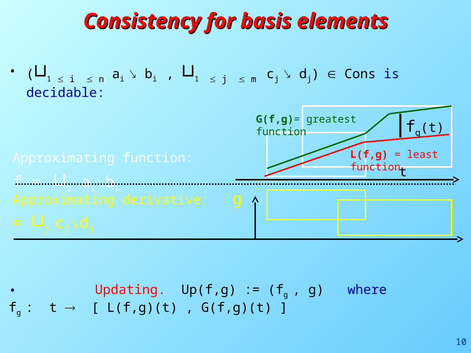
• Solve the ODE by iterating Up ⃘ Apv on D1 [-1,1]

starting with (f, t. v (t , f(t) ))

• Theorem. The domain-theoretic solution

⊔n 0 (Up ⃘ Apv )n (f, t. v (t , f(t) ))

is the unique classical solution through (0,0).

Function and Derivative UpgradingFunction and Derivative Upgrading

• Derivative upgrading:

Apv : ([-1,1] IR)2 ([-1,1] IR)2

(f,g) ( f , t. v (t , f(t) ))

• Function upgrading:

Up : ([-1,1] IR)2 ([-1,1] IR)2

Up(f,g) = (fg , g) where fg (t) = [ L (f,g) (t) , G (f,g) (t) ]

23

Computation of the solution for a given precision Computation of the solution for a given precision >0

• Let (un , wn) := (Pv )n (fn , t. vn (t , fn(t) ) ) with un = [un

- ,un+]n

• We express f and v as lubs of step functions:

f = ⊔n 0 fn v = ⊔n 0 vn

• Putting Pv := Up ⃘ Apv the solution is obtained as:

• For all n 0 we have: un- un+1

- un+1+ un

+ with un+ - un

- t. 0

• Compute the piecewise linear maps un- , un

+ until

the first n 0 with un+ - un

-

• ⊔n 0 (Pv )n (f , t. v (t , f(t) ) ) = ⊔n 0 (Pv )

n (fn , t. vn (t , fn(t) ) ) n

24

ExampleExample

1

f

g

1

1

1

v

v is approximated by a sequence of step functions, v0, v1, …

v = ⊔i vi

We solve: = v(t,x), x(t0) =x0

for t [0,1] with

v(t,x) = t and t0=1/2, x0=9/8.

dt

dx

a3

b3

a2

b2

a1

b1

v3

v2

v1

The initial condition is approximated by rectangles aibi:

{(1/2,9/8)} = ⊔i aibi,

t

t

.

25

SolutionSolution

1

f

g

1

1

1

At stage n we find un

- and un +

.

26

SolutionSolution

1

f

g

1

1

1 .

At stage n we find un

- and un +

27

SolutionSolution

1

f

g

1

1

1 un - and un

+ tend to

the exact solution:f: t t2/2 + 1

.

At stage n we find un

- and un +

28

Computing with polynomial step functionsComputing with polynomial step functions

29

Current and Further WorkCurrent and Further Work

• Implementation in Haskell

• Differential Calculus with Several Variables: PDE’s

• Construction of Smooth Curves and Surfaces

• Hybrid Systems, robotics,…

30

THE ENDTHE END

http://www.doc.ic.ac.uk/~aehttp://www.doc.ic.ac.uk/~ae