Embed Size (px)
Citation preview
CHAPTER 21
Structural Transformations and Market Failures inDevelopment
Together with the process of economic development and the changes in the structure ofproduction, there is also a transformation of the economy, which both involves major so-cial changes and induces greater (and perhaps more �complex�) coordination of economicactivities. Loosely speaking, we can think of a society that is relatively developed as func-tioning along (or at any rate, nearer) the frontier of its production possibilities set, while aless-developed economy may be in the interior of its �notional� production possibilities set.This may be because certain arrangements necessary for an economy to reach the frontier ofits production possibility set require a large amount of capital or some speciÞc technologicaladvances (in which case, even though we may think of the society as functioning in the inte-rior of its production possibility set, this may not be the outcome of market failure, thus thequaliÞer �notional� in the previous sentence). Alternatively, less developed economies maybe in the interior of their production possibility set because these societies are subject tosevere market failures. In this chapter, I discuss these approaches to economic development.
I Þrst focus on various dimensions of structural transformations and how these may belimited by the amount of capital or technology available in a society. I will then discussa number of approaches suggesting that less-developed economies might be su ering dis-proportionately from market failures or may even be �stuck� in �development traps�. Inthis context, I will also discuss di erences between models with multiple equilibria and withmultiple steady states.
The topics covered in this chapter are part of a large and diverse literature. My purposeis not to do justice to this literature, but to emphasize how certain major structural trans-formations take place as part of the process of economic development and also highlight thepotential importance of market failures in this process. Given this objective and the largenumber of potential models, my choice of models is selective and my treatment will be moreinformal than the rest of the book. In addition, I often make reduced-form assumptions inorder to keep the exposition brief and simple.
21.1. Financial Development
An important aspect of the structural transformation brought about by economic devel-opment is a change in Þnancial relations and deepening of Þnancial markets. Section 17.6in Chapter 17 already presented a model where economic growth goes hand-in-hand with
801
Introduction to Modern Economic Growth
Þnancial deepening. However, the model in that section only focused on a speciÞc aspect ofthe role of Þnancial institutions. In general, Þnancial development brings about a number ofcomplementary changes in the economy. First, there is greater depth in the Þnancial market,allowing better diversiÞcation of aggregate risks, a feature also emphasized in the model ofSection 17.6. Second, one of the key roles of Þnancial markets is to allow risk sharing andconsumption smoothing for individuals. In line with this, Þnancial development also allowsbetter diversiÞcation of idiosyncratic risks. Section 17.6 showed that better diversiÞcation ofaggregate risks leads to a better allocation of funds across sectors/projects. Similarly, bettersharing of idiosyncratic risks leads to a better allocation of funds across individuals. Third,Þnancial development might also reduce credit constraints on investors and thus may directlyenable the transfer of funds to individuals with better investment opportunities. The secondand the third channels not only a ect the allocation of resources in the society but also thedistribution of income, because diversiÞcation of idiosyncratic risks and relaxation of creditmarket constraints might lead to better income and risk sharing. On the other hand, as thepossibility of such risk-sharing arrangements reduce consumption risk, individuals might takeriskier actions, also potentially a ecting the distribution of income.
To provide a brief introduction to these issues, I now present a simple model of Þnan-cial development, focusing on the diversiÞcation of idiosyncratic risks and complementingthe analysis in Section 17.6. The model is inspired by the work of Townsend (1979) andGreenwood and Jovanovic (1990). It will illustrate how Þnancial development takes placeendogenously and interacts with economic growth, and will also provide some simple insightsabout the implications of Þnancial development for income distribution. Given the similarityof the model to that in Section 17.6, my treatment here will be relatively informal.
I consider an OLG economy in which each individual lives for two periods and has pref-erences given by
(21.1) E ( ( ) ( + 1)) = log ( ) + E log ( + 1)
where ( ) denotes the consumption of the unique Þnal good of the economy and E denotesthe expectation operator given time information.
There is no population growth and the total population of each generation is normalized to1. Let us assume that each individual is born with some labor endowment . The distributionof endowments across agents is given by the distribution function ( ) over some support£ ¤
This distribution of labor endowments is constant over time with mean = 1 and laboris supplied inelastically by all individuals in the Þrst period of their lives. In the secondperiod of their lives, individuals simply consume their capital income.
The aggregate production function of the economy is given by
( ) = ( ) ( )1 = ( )
where (0 1) and the second equality uses the fact that total labor supply will be equalto 1 at each date. As in Section 17.6, the only risk is in transforming savings into capital,
802
Introduction to Modern Economic Growth
thus the lifecycle of an individual looks identical to that shown in Figure 17.3 in that section.Moreover, suppose that agents can either save all of their labor earnings from the Þrst periodof their lives using a safe technology with rate of return (in terms of capital at the nextdate) or invest all of their labor income in the risky technology with return + , whereis a mean zero independently and identically distributed stochastic shock and as in Section17.6, we assume that . This implies that the risky technology is more productive. Theassumption that individuals have to choose one of these two technologies rather than dividingtheir savings between the two is made for simplicity (see Exercise 21.1).
Although the model looks very similar to that in Section 17.6, there is a crucial di erence.Because is identically and independently distributed across individuals, if individuals couldpool their resources, they could perfectly diversify idiosyncratic risks. In particular, if a largenumber (a continuum) of individuals pooled their resources, they would guarantee an averagereturn of . Let us assume that this is not possible because of a standard informationalproblem�the actual return of an individual�s saving decision is not observed by others unlesssome Þnancial monitoring is undertaken. Let us assume that this type of Þnancial monitoringcosts 0 for each individual. This implies that by paying the cost of , each individualcan join the Þnancial market (or in the language of Townsend, he can become part of a�Þnancial coalition�). In this case, the actual returns of his savings become fully observable.Intuitively, this cost captures the Þxed costs that individuals have to pay to be engaged inÞnancial markets as well as the Þxed costs associated with monitoring or being monitored.An immediate implication of this speciÞcation is that joining the Þnancial markets is moreattractive for richer individuals, since the Þxed cost is less important for them. This featureis both plausible and also generates predictions consistent with microdata, where we observericher individuals investing in more complex Þnancial securities.
If an individual does not join the Þnancial markets, then no other agent in the economycan observe the realization of the returns on his savings. In this case, no Þnancial contractfor sharing of idiosyncratic risks is possible, since such a contract would involve agents thathave a high (realized) value of making transfers to those who are unlucky and have lowrealized values of . However, without monitoring, each agent will claim to have a low valueof , thus receive ex post payments. The anticipation of this type of opportunistic behaviorprevents any risk sharing in the absence of monitoring.
Let us also assume that has a distribution with positive probability of = , so thatif an individual undertakes the risky investments, there is a positive probability that all hissavings will be lost. This implies that without some type of risk sharing, individuals willchoose the safe project. This observation simpliÞes the analysis of the model. Suppose thatthe economy starts with some initial capital stock of (0) 0, so an individual with laborendowment will have labor earnings of (0) = (0) , where
(21.2) ( ) = (1 ) ( )
803
Introduction to Modern Economic Growth
is the competitive wage rate at time . After labor incomes are realized, individuals Þrst maketheir savings decisions and then choose which assets to invest in. The preferences in (21.1)imply that individuals will save a constant fraction (1 + ) of their income regardlessof their income level or the rate of return (in particular, independent of whether they areinvesting in the risky or the safe asset). In view of this, the value to not participating in theÞnancial markets for individual at time is
( ( ) ( + 1)) = logµ
11 +
( )¶+ log
µ( + 1)1 +
( )
which takes into account that the rate of return on capital in the second period of the life ofthe individual will be ( + 1) and the individual will receive a gross return on his savings of
( ) (1 + ). Next, suppose that there are su ciently many (that is, a positive measureof) other individuals taking part in Þnancial markets. Then, when the individual decides totake part in Þnancial markets, his value will be
( ( ) ( + 1)) = logµ
11 +
( ( ) )¶+ log
µ( + 1)1 +
( ( ) )
which takes into account that the individual will have to spend the amount out of his laborincome on the cost of joining the Þnancial market, leaving him a net income of ( ) .He will then save a fraction (1 + ) of this, but in return, he will receive the higherreturn for sure. The reason why the individual receives , rather than a risky return, isbecause, conditional on joining the Þnancial market, each individual is able to fully diversifyhis idiosyncratic risks. The comparison of these two expressions gives the threshold level
(21.3)1 ( ) (1+ )
0
such that individuals with Þrst-period earnings greater than will join the Þnancial marketand those with less than will not. A notable feature of this threshold is that it isindependent of the rate of return on capital in the second period of the lives of the individuals,. This is an implication of log preferences in (21.1).Given the behavior of individuals concerning whether they will join the Þnancial market,
let us next determine the evolution of the economy by studying the evolution of individualearnings. Individual earnings are determined by two factors: labor endowments and thecapital stock at time , which gives the wage per unit of labor, ( ), as in (21.2). Given( ), the fraction of individuals who will join the Þnancial market at time , ( ), is given
by the fraction of individuals who have ( ). Alternatively, using the fact thatlabor endowments have a distribution given by (·), the fraction of individuals investing inÞnancial markets is obtained as
(21.4) ( ) 1µ
( )
¶= 1
µ
(1 ) ( )
804
Introduction to Modern Economic Growth
In view of this and deÞning ( ) (1 ) ( ) , the capital stock at time + 1 canbe written as
(21.5) ( + 1) =1 +
" Z ( )( ) +
Z
( )( ) ( )
#(1 ) ( )
which takes into account that all individuals with labor endowment less than ( ) choose thesafe project and receive the gross return on their savings, while those above this thresholdspend on monitoring and receive the higher return . It can be veriÞed that ( + 1) isincreasing in ( ) and there will be growth in the capital stock (and thus output) of theeconomy provided that ( ) is less than the �steady-state� level of capital; see Exercise21.2).
Now inspection of the accumulation equation (21.5) together with the threshold rule forjoining the Þnancial market leads to a number of interesting conclusions.
1. As ( ) increases, that is, as the economy develops, equation (21.4) implies that moreindividuals will join the Þnancial market. Consequently, a greater level of capital will leadto more risk taking, but these risks will also be shared better. More importantly, economicdevelopment also induces a better composition of investment as a greater fraction of theindividuals start using their savings more e ciently. Thus with a mechanism similar to thatin Section 17.6, economic development improves the allocation of funds in the economy andincreases productivity. Consequently, this model, like the one in Section 17.6, implies thateconomic development and Þnancial development go hand-in-hand.
2. However, there is also a distinct sense in which the economy here allows for a po-tential causal e ect of Þnancial development on economic growth. Imagine that societiesdi er according to their �s, which can be interpreted as a measure of the institutionally- ortechnologically-determined costs of monitoring or some other costs associated with Þnancialtransactions that may depend on the degree of investor protection. Societies with lower �swill have a greater participation in Þnancial markets and this will endogenously increase theirproductivity. Thus, while the equilibrium behavior of Þnancial and economic developmentare jointly determined, di erences in Þnancial development driven by exogenous institutionalfactors related to will have a potential causal e ect on economic growth.
3. As noted above, at any given point in time it will be the richer agents�those withgreater labor endowment�that will join the Þnancial market. Therefore, initially, the Þnan-cial market will help those who are already well-o to increase the rate of return on theirsavings. This can be thought of as the unequalizing e ect of the Þnancial market.
4. The fact that participation in Þnancial markets increases with ( ) also implies thatas the economy grows, at least at the early stages of economic development, the unequalizinge ect of Þnancial intermediation will become stronger. Therefore, presuming that the econ-omy starts with relatively few rich individuals, the Þrst expansion of the Þnancial market willincrease the level of overall inequality in the economy as a greater fraction of the agents inthe economy now enjoy the greater returns.
805
Introduction to Modern Economic Growth
5. As ( ) increases even further, eventually the equalizing e ect of the Þnancial marketstarts operating. At this point, the fraction of the population joining the Þnancial marketand enjoying the greater returns is steadily increasing. If the steady-state level of capitalstock is such that (1 ) ( ) , then eventually all individuals will join theÞnancial market and receive the same rate of return on their savings.
The last two observations are interesting in part because the relationship between growthand inequality is a topic of great interest to development economics (one to which I returnlater in this chapter). One of the most important ideas in this context is that of the Kuznetscurve, which claims that economic growth Þrst increases and then reduces income inequalityin the society. Whether the Kuznets curve is a good description of the relationship betweengrowth and inequality is a topic of current debate. While many European societies seemto have gone through a phase of increasing and then decreasing inequality during the 19thcentury, the evidence for the 20th century is more mixed. The last two observations showthat a model with endogenous Þnancial development based on risk sharing among individualscan generate a pattern consistent with the Kuznets curve. Whether there is indeed a Kuznetscurve in general, and if so, whether the mechanism highlighted here plays an important rolein generating this pattern are areas for future theoretical and empirical work.
21.2. Fertility, Mortality and the Demographic Transition
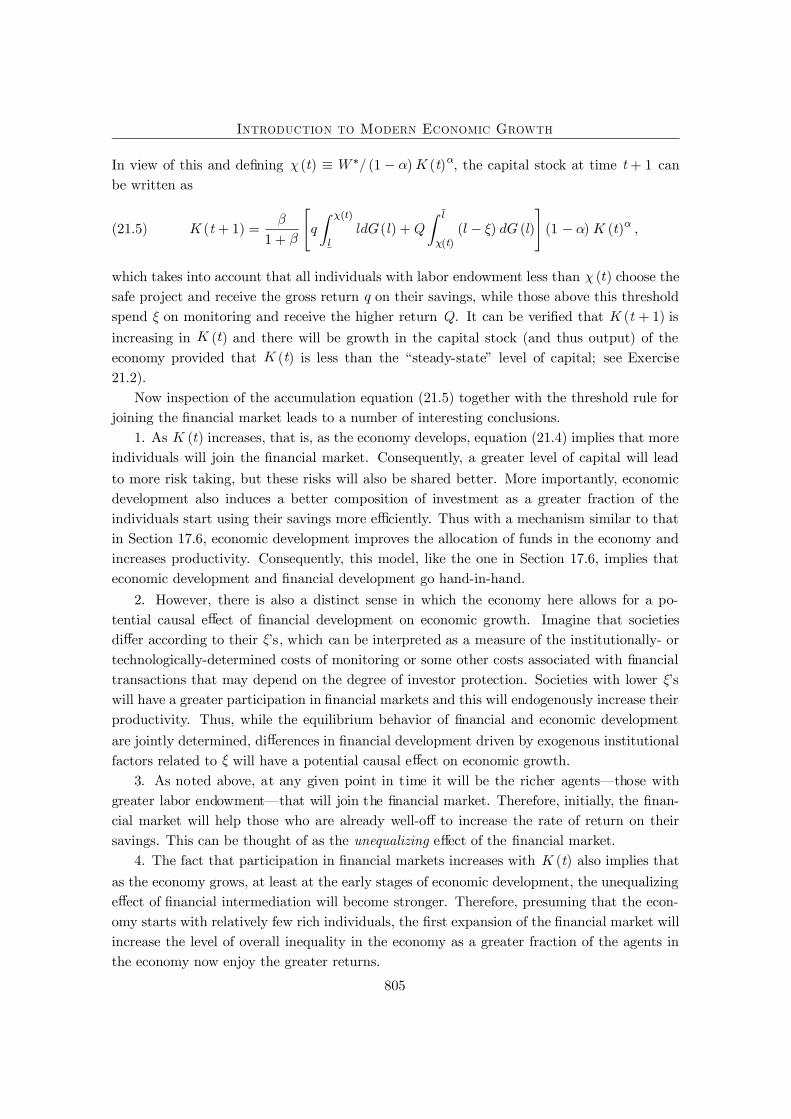
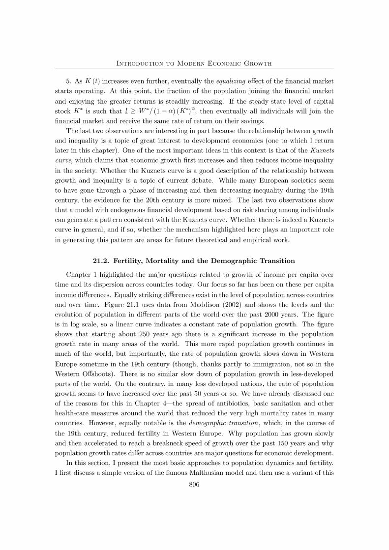
Chapter 1 highlighted the major questions related to growth of income per capita overtime and its dispersion across countries today. Our focus so far has been on these per capitaincome di erences. Equally striking di erences exist in the level of population across countriesand over time. Figure 21.1 uses data from Maddison (2002) and shows the levels and theevolution of population in di erent parts of the world over the past 2000 years. The Þgureis in log scale, so a linear curve indicates a constant rate of population growth. The Þgureshows that starting about 250 years ago there is a signiÞcant increase in the populationgrowth rate in many areas of the world. This more rapid population growth continues inmuch of the world, but importantly, the rate of population growth slows down in WesternEurope sometime in the 19th century (though, thanks partly to immigration, not so in theWestern O shoots). There is no similar slow down of population growth in less-developedparts of the world. On the contrary, in many less developed nations, the rate of populationgrowth seems to have increased over the past 50 years or so. We have already discussed oneof the reasons for this in Chapter 4�the spread of antibiotics, basic sanitation and otherhealth-care measures around the world that reduced the very high mortality rates in manycountries. However, equally notable is the demographic transition, which, in the course ofthe 19th century, reduced fertility in Western Europe. Why population has grown slowlyand then accelerated to reach a breakneck speed of growth over the past 150 years and whypopulation growth rates di er across countries are major questions for economic development.
In this section, I present the most basic approaches to population dynamics and fertility.I Þrst discuss a simple version of the famous Malthusian model and then use a variant of this
806
Introduction to Modern Economic Growth
Asia
Western Offshoots
Europe
Africa
Latin America10000
50000
500000
2000000
5000000
0 500 1000 1500 2000Year
Figure 21.1. Total population in di erent parts of the world over the past2000 years.
model to investigate potential causes of the demographic transition. Thomas Malthus wasone of the most brilliant and inßuential economists of the 19th century and is responsible forone of the Þrst general equilibrium growth models. The next subsection will present a versionof this model. The Malthusian model is responsible for earning the discipline of economicsthe name �the dismal science� because of its dire prediction that population will adjust up ordown (by births or deaths) until all individuals are at the subsistence level of consumption.Nevertheless, this dire prediction is not the most important part of the Malthusian model.Instead, at the heart of this model is the negative relationship between income per capita andpopulation, which is itself endogenously determined. In this sense, it is closely related to theSolow and the neoclassical growth models, augmented with a behavioral rule that determinesthe rate of population growth. It is this less extreme version of the Malthusian model thatwill be presented in the next subsection. I then enrich this model by the important andinßuential idea due to Gary Becker that there is a tradeo between the quantity and qualityof children and that this tradeo changes over the process of development. I show how asimple model can incorporate the notion that over the course of development parents maystart valuing the quality (human capital) of their o spring more and how this may lead to apattern reminiscent to the demographic transition.
21.2.1. A Simple Malthusian Model. Consider the following non-overlapping gen-erations model that starts with a population of (0) 0 at time = 0. A representative
807
Introduction to Modern Economic Growth
individual living at time supplies one unit of labor inelastically and has utility
(21.6) ( ) ( + 1) ( + 1)12 0 ( + 1)2
¸
where ( ) denotes the consumption of the unique Þnal good of the economy by the individualhimself, ( + 1) denotes the number of o spring the individual begets and ( + 1) is theincome of each o spring, and 0 and 0 0. The last term in square brackets is the child-rearing costs and is assumed to be convex to reßect the fact that the costs of having more andmore children will be higher (for example, because of time constraints of parents, though onecan also make arguments for why the costs of child-rearing might exhibit increasing returnsto scale over a certain range). Clearly, these preferences introduce a number of simplifyingassumptions. First, each individual is allowed to have as many o spring as he likes, whichis unrealistic because it does not restrict the number of o spring to a natural number. Thetechnology also does not incorporate possible specialization in child-rearing and market workwithin the family. Second, these preferences introduce the �warm glow� type altruism weencountered in Chapter 9, so that parents receive utility not from the future utility of theiro spring, but from some characteristic of their o spring. Here it is a transform of the totalincome of all the o spring that features in the utility function of the parent. Third, the costsof child-rearing are in terms of �utils� rather than forgone income, and current consumptionmultiplies both the beneÞts and the costs of having additional children. This feature, whichis motivated by balanced growth type reasoning, implies that the demand for children will beindependent of current income (otherwise, growth will automatically lead to greater demandfor children). All three of these assumptions are adopted for simplicity. I have also writtenthe number of o spring that an individual has a time as ( + 1), since this will determinepopulation at time + 1.
Each individual has one unit of labor and there are no savings. The production functionfor the unique good takes the form
(21.7) ( ) = ( )1
where is the total amount of land available for production and ( ) is total labor supply.There is no capital and land is introduced in order to create diminishing returns to labor,which is an important element of the Malthusian model. Without loss of generality, I normal-ize the total amount of land to = 1. A key question in models of this sort is what happensto the returns to land. The most satisfactory way of dealing with this problem would beto allocate the property rights to land among the individuals and let them bequeath this totheir o spring. This, however, introduces another layer of complication, and since my pur-pose here is to illustrate the basic ideas, I follow the unsatisfactory assumption often madein the literature, that land is owned by another set of agents, whose behavior will not beanalyzed here.
By deÞnition, population at time + 1 is given as
(21.8) ( + 1) = ( + 1) ( )
808
Introduction to Modern Economic Growth
which takes into account new births as well as the death of the parent.Labor markets are competitive, so the wage at time + 1 is given as
(21.9) ( + 1) = (1 ) ( + 1)
Since there is no other source of income, this is also equal to the income of each individualliving at time + 1, ( + 1). Thus an individual with income ( ) at time will solvethe problem of maximizing (21.6) subject to the constraint that ( ) ( ), together with( + 1) = (1 ) ( + 1) . Naturally, in equilibrium ( + 1) must be consistent with( + 1) according to equation (21.8). Individual maximization implies
( + 1) = (1 ) 10 ( + 1)
Now substituting for (21.8) and rearranging, we obtain
(21.10) ( + 1) = (1 )1
1+1
1+0 ( )
11+
This equation implies that ( + 1) is an increasing concave function of ( ). In fact, thelaw of motion for population implied by (21.10) resembles the dynamics of capital-labor ratioin the Solow growth model (or the OLG model) and is plotted in Figure 21.2. The Þguremakes it clear that starting with any (0) 0, there exists a unique globally stable statestate given by
(21.11) (1 )1 10
If the economy starts with (0) , then population will slowly (and monotonically) adjusttowards this steady-state level. Moreover, (21.9) shows that as population increases wagesfall. If in contrast, (0) , then the society experiences a decline in population and risingreal wages. It is straightforward to introduce shocks to population and show that in this case,the economy will ßuctuate around the steady-state population level (with an invariantdistribution depending on the distribution of the shocks) and experience cycles reminiscentto the Malthusian cycles, with periods of increasing population and decreasing wages followedby periods of decreasing population and increasing wages (see Exercise 21.3).
The main di erence of this model from the simplest (or the crudest) version of the Malthu-sian model is that there is no biologically determined subsistence level of consumption. Thesteady-state level of consumption instead reßects technology and preferences, and is given by
= (1 ) ( ) = 0
21.2.2. The Demographic Transition. To study the demographic transition, I nowintroduce a quality-quantity tradeo along the lines of the ideas suggested by Gary Becker.Each parent can choose his o spring to be unskilled or skilled. To make them skilled, theparent has to exert the additional e ort for child-rearing denoted by ( ) {0 1}. If hechooses not to do this, his o spring will be unskilled.
The total population of unskilled individuals at time is denoted by ( ) and the totalpopulation of the skilled is denoted by ( ), clearly with
( ) = ( ) + ( )
809
Introduction to Modern Economic Growth
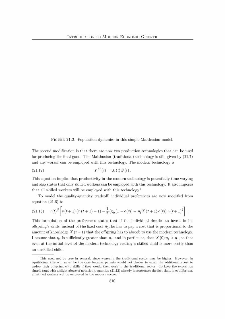
Figure 21.2. Population dynamics in this simple Malthusian model.
The second modiÞcation is that there are now two production technologies that can be usedfor producing the Þnal good. The Malthusian (traditional) technology is still given by (21.7)and any worker can be employed with this technology. The modern technology is
(21.12) ( ) = ( ) ( )
This equation implies that productivity in the modern technology is potentially time varyingand also states that only skilled workers can be employed with this technology. It also imposesthat all skilled workers will be employed with this technology.1
To model the quality-quantity tradeo , individual preferences are now modiÞed fromequation (21.6) to
(21.13) ( ) ( + 1) ( ( + 1) 1)12( 0 (1 ( )) + 1 ( + 1) ( )) ( + 1)2
¸
This formulation of the preferences states that if the individual decides to invest in hiso spring�s skills, instead of the Þxed cost 0, he has to pay a cost that is proportional to theamount of knowledge ( + 1) that the o spring has to absorb to use the modern technology.I assume that 1 is su ciently greater than 0, and in particular, that (0) 1 0, so thateven at the initial level of the modern technology rearing a skilled child is more costly thanan unskilled child.
1This need not be true in general, since wages in the traditional sector may be higher. However, inequilibrium this will never be the case because parents would not choose to exert the additional e ort toendow their o spring with skills if they would then work in the traditional sector. To keep the expositionsimple (and with a slight abuse of notation), equation (21.12) already incorporates the fact that, in equilibrium,all skilled workers will be employed in the modern sector.
810
Introduction to Modern Economic Growth
Finally, I assume learning-by-doing is external as in Romer (1986a), so that
(21.14) ( + 1) = ( )
which implies that the improvement in the technology of the modern sector is a function ofthe number of skilled workers employed in this sector. This type of reduced-form assumptionis clearly unsatisfactory, but as noted above, one could get similar results with an endogenoustechnology model with the market size e ect. Another important feature of this productionfunction is that it does not use land. This assumption is consistent with the fact that mostmodern production processes make little use of land, instead relying on technology, physicalcapital and human capital.
The output of the traditional and the modern sectors are perfect substitutes�they bothproduce the same Þnal good. In view of the observation that all unskilled workers will work inthe traditional sector and all skilled workers will work in the modern sector, wages of skilledand unskilled workers at time are
(21.15) ( ) = (1 ) ( ) and
(21.16) ( ) = ( )
where (21.15) is identical to (21.9) in the previous subsection, except that it features onlythe unskilled workers instead of the entire labor force.
Let us next turn to the fertility and quality-quantity decisions of individuals. As before,current income has no e ect on fertility and quality-quantity decisions. Thus we do not needto distinguish between high-skill and low-skill parents. Using this observation, let us simplylook at the optimal number of o spring that an individual will have when he chooses ( ) = 0.This is given by
(21.17) ( + 1) = ( + 1) 10 = (1 ) ( + 1) 1
0
where the second line uses (21.15). Instead, if the parent decides to exert e ort ( ) = 1 andinvest in the skills of his o spring, then he will choose the number of o spring equal to
(21.18) ( + 1) = ( + 1) ( + 1) 1 11 = 1
1
The comparison of equations (21.17) and (21.18) suggests that unless unskilled wages arevery low, an individual who decides to provide additional skills to his o spring will havefewer o spring. This is because bringing up skilled children is more expensive (i.e., because
1 is su ciently larger than 0). Thus the comparison of these two equations captures thequality-quantity tradeo .
Substituting these equations back into the utility function (21.13), we obtain the utilityfrom the two strategies (normalized by consumption, that is, the utility divided by ( ) ) as
( ) =12(1 )2 ( + 1) 2 1
0 and ( ) =12
( + 1) 11
811
Introduction to Modern Economic Growth
Inspection of these two expressions shows that in equilibrium, some workers must be unskilled,since otherwise would become inÞnite. Therefore, in equilibrium
(21.19) ( ) ( )
This equilibrium condition implies that there are two possible conÞgurations. First, (0)can be so low that (21.19) will hold as a strict inequality. In this case, all individuals will beunskilled. The condition for this inequality to be strict is
(0) 11 (1 )2 (1) 2 1
0
which uses the fact that when there are no skilled workers, there is no production in themodern sector and thus (1) = (0). If this inequality satisÞed, there would be no skilledchildren at date = 0. However, as long as (1) is less than as given in (21.11), populationwill grow. It is therefore possible that at some point (21.19) holds with equality. The conditionfor this never to happen is that
(21.20) (0) 11 (1 )2 ( ) 2 1
0
In this case, the law of motion of population is identical to that in the previous subsection andthere is never any investment in skills. We can think of this is a pure Malthusian economy.
If, on the other hand, condition (21.20) is not satisÞed, then at least at some pointindividuals will start investing in the skills of their o spring. From then on, (21.19) musthold as equality. Let the fraction of parents having unskilled children at time be denotedby ( + 1). Then, by deÞnition
( + 1) = ( + 1)¡
( + 1) 1¢( )
= ( + 1)1 (1+ ) (1 )2 (1+ ) 1 (1+ )0 ( )1 (1+ )(21.21)
and
( + 1) = (1 ( + 1))¡
( + 1) 1¢( )
= (1 ( + 1)) 11 ( )(21.22)
Moreover, to satisfy (21.19) as equality, we need (1 )2 ( + 1) 2 10 = ( + 1) 1
1 ,or rearranging
(21.23) ( + 1) 11 = ( + 1) 2 (1+ ) (1 )2(1 ) (1+ ) (1 ) (1+ )
0 ( ) 2 (1+ )
Equilibrium dynamics are then determined by equations (21.21)-(21.23) together with (21.16).While the details of the behavior of this dynamical system are somewhat involved, the generalpicture is clear. Most interestingly, if an economy starts with both a low level of (0) anda low level of (0), but does not satisfy condition (21.20), then the economy will start inthe Malthusian regime, only making use of the traditional technology and not investing inskills. As population increases wages fall, and at that point parents start Þnding it beneÞcialto invest in the skills of their children and Þrms start using the modern technology. Parentsthat invest in the skills of their children will typically have fewer children than parentsrearing unskilled o spring (because 1 is su ciently larger than 0, (21.17) will be greater
812
Introduction to Modern Economic Growth
than (21.18)). The aggregate rate of population growth and fertility are still high at Þrst,but as the modern technology improves and the demand for skills increases, a larger fractionof parents start investing in the skills of their children and the rate of population growthdeclines. Ultimately, the rate of population growth approaches 1
1 . This model thus gives astylized representation of the demographic transition based on quality-quantity trade-o .
There are substantially richer models of the demographic transition in the literature. Forexample, there are many ways of introducing quality-quantity tradeo s, and what spurs achange in the quality-quantity tradeo may be an increase in capital intensity of production,changes in the wages of workers, or changes in the wages of women di erentially a ectingthe desirability of market and home activities. Nevertheless, the general qualitative featuresare similar in that the quality-quantity tradeo is often viewed as the major reason for thedemographic transition. Despite this emphasis on the quality-quantity tradeo , there isrelatively little direct evidence that this tradeo is important in general or in leading to thedemographic transition. Other social scientists have suggested social norms, the large declinesin mortality starting in the 19th century, or the reduced need for child labor as potentialfactors contributing to the demographic transition. As of yet, there is no general consensuson the causes of the demographic transition or on the role of the quality-quantity tradeoin determining population dynamics. The study of population growth and demographictransition is an exciting and important area, and theoretical and empirical analyses of thefactors a ecting fertility decisions and how they interact with the reallocation of workersacross di erent tasks (sectors) remain important and interesting questions to be explored.
21.3. Migration, Urbanization and The Dual Economy
Another major structural transformation over the process of development relates tochanges in social and living arrangements. For example, as an economy develops, moreindividuals move from rural areas to cities and also undergo the social changes associatedwith separation from a small community and becoming part of a larger, more anonymousenvironment. Other social changes might also be important. For instance, certain socialscientists regard the replacement of �collective responsibility systems� by �individual respon-sibility systems� as an important social transformation. This is clearly related to changes inthe living arrangements of individuals (e.g., villages versus cities, or extended versus nuclearfamilies). It is also linked to whether di erent types of contracts are being enforced by so-cial norms and community enforcement, or whether they are enforced by legal institutions.There may also be a similar shift in the importance of the market, as more activities aremediated via prices rather than taking place inside the home or using the resources of anextended family or a broader community. This process of social change is both complex andinteresting to study, though a detailed discussion of the literature and possible approachesto these issues falls beyond the scope of the current book.
813
Introduction to Modern Economic Growth
Nevertheless, a brief discussion of some of these social changes are useful to illustrateother, more diverse facets of structural transformations associated with economic develop-ment. I illustrate the main ideas by focusing on the process of migration from rural areas andurbanization. Another reason to study migration and urbanization is that the reallocation oflabor from rural to urban areas is closely related to the popular concept of the dual economy ,which is an important theme of some of the older literature on development economics. Ac-cording to this notion, less-developed economies consist of a modern sector and a traditionalsector, but the connection between these two sectors is imperfect. The model of industri-alization in the previous chapter (Section 20.3) featured a traditional and a modern sector,but these sectors traded their outputs and competed for labor in competitive markets. Dualeconomy approaches, instead, emphasize situations in which the traditional and the modernsectors function in parallel, but with only limited interactions. Moreover, the traditionalsector is often viewed as less e cient than the modern sector, thus the lack of interactionmay also be a way of shielding the traditional economy from its more e cient competitor. Anatural implication of this approach will then be to view the process of development as onein which the less e cient traditional sector is replaced by the more e cient modern sector.Lack of development may in turn correspond to an inability to generate such reallocation.
In this section I Þrst present a model of migration that builds on the work by Arthur Lewis(1954). A less-developed economy is modeled as a dual economy, with the traditional sectorassociated with villages and the modern sector with the cities. I then present a model inspiredby Banerjee and Newman (1998) and Acemoglu and Zilibotti (1999), in which the traditionalsector and the rural economy have a comparative advantage in community enforcement, eventhough in line with the other dual economy approaches, the modern economy (the city)enables the use of more e cient technologies. This model also illustrates how certain aspectsof the traditional sector can shield the less productive Þrms from more productive competitorsand slow down the process of development. Finally, I show how the import of technologiesfrom more developed economies, along the lines of the models discussed in Section 18.4 ofChapter 18, may also lead to dual economy features as a byproduct of the introduction ofmore skill-intensive, modern technologies into less-developed economies.
21.3.1. Surplus Labor and the Dual Economy. Lewis argued that less-developedeconomies typically had surplus labor, that is, unemployed or underemployed labor, oftenin the villages. The dual economy can then be viewed as the juxtaposition of the modernsector, where workers are productively employed, with the traditional sector, where they areunderemployed. The general tendency of less-developed economies to have lower levels ofemployment to population ratios was one of the motivations for Lewis�s model. A key featureof Lewis�s model is the presence of some barriers preventing, or slowing down, the allocationof workers away from the traditional sector towards urban areas, and the modern sector. Inow present a reduced-form model that formalizes these notions.
Consider a continuous-time inÞnite-horizon economy that consists of two sectors or re-gions, which I refer to as urban and rural. Total population is normalized to 1. At time
814
Introduction to Modern Economic Growth
= 0, (0) individuals are in the urban area and (0) = 1 (0) are in the rural area.In the rural area, the only economic activity is agriculture and, for simplicity, suppose thatthe production function for agriculture is linear, thus total agricultural output is
( ) = ( )
where 0. In the urban area, the main economic activity is manufacturing. Manufactur-ing can only employ workers in the urban area and will employ all of the available workers.The production function therefore takes the form
( ) =¡( ) ( )
¢
where ( ) is the capital stock, with initial condition (0). is a standard neoclassicalproduction function satisfying Assumptions 1 and 2. Let us also assume, for simplicity, thatthe manufacturing and the agricultural goods are perfect substitutes. Labor markets both inthe rural and urban area are competitive. There is no technological change in either sector.
The key assumption is that because of barriers to mobility, there will only be slow migra-tion of workers from rural to urban areas even when manufacturing wages are greater thanrural wages. In particular, let us capture the dynamics in this model in a reduced-form waywhereby capital accumulates only out of the savings of individuals in the urban area, thus
(21.24) ú ( ) =¡
( ) ( )¢
( )
where is the exogenous saving rate and is the depreciation rate of capital. The importantfeature implied by this speciÞcation is that greater output in the modern sector leads tofurther accumulation of capital for the modern sector. An alternative, adopted in Section20.3 of the previous chapter that will also be used in the next subsection, is to allow the sizeof the modern sector to directly inßuence its productivity growth, for example because oflearning-by-doing externalities as in Romer (1986a) or because of endogenous technologicalchange depending on the market size commanded by this sector (e.g., Exercise 20.19). Forthe purposes of the model in this subsection, which of these alternatives is adopted has nomajor consequences.
Given competitive labor markets, the wage rates in the urban and rural areas are
( ) =¡
( ) ( )¢and ( ) =
Let us assume that
(21.25)( (0) 1)
so that even if all workers are employed in the manufacturing sector at the initial capitalstock, they will have a higher marginal product than working in agriculture.
Migration dynamics are assumed to take the following simple form:
(21.26) ú ( )= ( ) if ( ) ( )£
( ) 0¤if ( ) = ( )
= 0 if ( ) ( )
815
Introduction to Modern Economic Growth
This equation implies that as long as wages in the urban sector are greater than those in therural sector, there is a constant rate of migration. The speed of migration does not dependon the wage gap, which is an assumption adopted only to simplify the exposition. We maywant to think of as small, so that there are barriers to migration and even when there aresubstantial gains to migrating to the cities, migration will take place slowly. When there isno wage gain to migrating, there will be no migration.
Now (21.25) implies that at date = 0, there will be migration from the rural areastowards the cities. Moreover, assuming that (0) (0) is below the steady-state capital-labor ratio, the wage will remain high and will continue to attract further workers. To analyzethis process in slightly greater detail, let us deÞne
(0)(0)(0)
as the capital-labor ratio in manufacturing (the modern sector). As usual, let us also de-Þne the per capita production function in manufacturing as ( ( )). Clearly, ( ) =( ( )) ( ) 0 ( ( )). Combining (21.24) and (21.26), we obtain that, as long as( ( )) ( ) 0 ( ( )) , the dynamics of this capital-labor ratio will be given by
(21.27) ú ( ) = ( ( )) ( + ( )) ( )
where ( ) ( ) ( ) is the ratio of the rural to urban population. Notice that whenurban wages are greater than rural wages, the rate of migration, , times the ratio ( ),plays the role of the rate of population growth in the basic Solow model. In contrast, when( ( )) ( ) 0 ( ( )) , there is no migration and
(21.28) ú ( ) = ( ( )) ( )
Let us focus on the former case. DeÞne the level of capital-labor ratio ¯ such that urban andrural wages are equalized. This is given by
(21.29) (¯) ¯ 0(¯) =
Once this level is reached, migration stops and ( ) remains constant. After this level,equilibrium dynamics are given by (21.28). Therefore, the steady state must involve
(21.30)(�)� =
For the analysis of transitional dynamics, which are our primary interest here, there areseveral cases to study. Let us focus on the one that appears most relevant for the experiencesof many less-developed economies (leaving the rest to Exercise 21.4). In particular, supposethat the following conditions hold:
1. (0) �, so that the economy starts with lower capital-labor ratio (in the urbansector) than the steady-state level. This assumption also implies that ( (0)) (0) 0.
2. (0) ¯, which implies that ( (0)) (0) 0 ( (0)) , that is, wages are initiallyhigher in the urban sector than in the rural sector.
816
Introduction to Modern Economic Growth
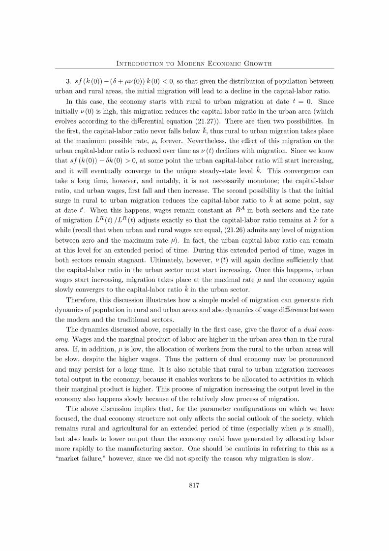
3. ( (0)) ( + (0)) (0) 0, so that given the distribution of population betweenurban and rural areas, the initial migration will lead to a decline in the capital-labor ratio.
In this case, the economy starts with rural to urban migration at date = 0. Sinceinitially (0) is high, this migration reduces the capital-labor ratio in the urban area (whichevolves according to the di erential equation (21.27)). There are then two possibilities. Inthe Þrst, the capital-labor ratio never falls below ¯, thus rural to urban migration takes placeat the maximum possible rate, , forever. Nevertheless, the e ect of this migration on theurban capital-labor ratio is reduced over time as ( ) declines with migration. Since we knowthat ( (0)) (0) 0, at some point the urban capital-labor ratio will start increasing,and it will eventually converge to the unique steady-state level �. This convergence cantake a long time, however, and notably, it is not necessarily monotone; the capital-laborratio, and urban wages, Þrst fall and then increase. The second possibility is that the initialsurge in rural to urban migration reduces the capital-labor ratio to ¯ at some point, sayat date 0. When this happens, wages remain constant at in both sectors and the rateof migration ú ( ) ( ) adjusts exactly so that the capital-labor ratio remains at ¯ for awhile (recall that when urban and rural wages are equal, (21.26) admits any level of migrationbetween zero and the maximum rate ). In fact, the urban capital-labor ratio can remainat this level for an extended period of time. During this extended period of time, wages inboth sectors remain stagnant. Ultimately, however, ( ) will again decline su ciently thatthe capital-labor ratio in the urban sector must start increasing. Once this happens, urbanwages start increasing, migration takes place at the maximal rate and the economy againslowly converges to the capital-labor ratio � in the urban sector.
Therefore, this discussion illustrates how a simple model of migration can generate richdynamics of population in rural and urban areas and also dynamics of wage di erence betweenthe modern and the traditional sectors.
The dynamics discussed above, especially in the Þrst case, give the ßavor of a dual econ-omy. Wages and the marginal product of labor are higher in the urban area than in the ruralarea. If, in addition, is low, the allocation of workers from the rural to the urban areas willbe slow, despite the higher wages. Thus the pattern of dual economy may be pronouncedand may persist for a long time. It is also notable that rural to urban migration increasestotal output in the economy, because it enables workers to be allocated to activities in whichtheir marginal product is higher. This process of migration increasing the output level in theeconomy also happens slowly because of the relatively slow process of migration.
The above discussion implies that, for the parameter conÞgurations on which we havefocused, the dual economy structure not only a ects the social outlook of the society, whichremains rural and agricultural for an extended period of time (especially when is small),but also leads to lower output than the economy could have generated by allocating labormore rapidly to the manufacturing sector. One should be cautious in referring to this as a�market failure,� however, since we did not specify the reason why migration is slow.
817
Introduction to Modern Economic Growth
21.3.2. Community Enforcement, Migration and Development. I now present amodel inspired by Banerjee and Newman (1998) and Acemoglu and Zilibotti (1999). Baner-jee and Newman consider an economy where the traditional sector has low productivity butis less a ected by informational asymmetries and thus individuals can engage in borrowingand lending with limited monitoring and incentive costs. In contrast, the modern sectoris more productive, but informational asymmetries create more severe credit market prob-lems. Banerjee and Newman discuss how the process of development is associated with thereallocation of economic activity from the traditional to the modern sector and how this real-location is slowed down by the informational advantage of the traditional sector. Acemogluand Zilibotti (1999) view the development process as one of �information accumulation,�and greater information enables individuals to write more sophisticated contracts and enterinto more complex production relations. This process is then associated with changes intechnology, changes in Þnancial relations and social transformations, since greater availabil-ity of information and better contracts enable individuals to abandon less e cient and lessinformation-dependent social and productive relationships.
The model in this subsection is simpler than both of these papers, but features a similareconomic mechanism. Individuals who live in rural areas are subject to community enforce-ment. This means that they can enter into economic and social relationships without beingunduly a ected by moral hazard problems. When individuals move to cities, they can takepart in more productive activities, but other enforcement systems are necessary to ensurecompliance to social rules, contracts and norms. These systems will typically be associatedwith certain costs. As in the model of industrialization in the previous section, I also assumethat the modern sector is subject to learning-by-doing externalities. Thus the productivityadvantage of the modern sector grows as more individuals migrate to cities and work there.However, the community enforcement advantage of villages slows down this process.
Both labor markets are competitive and total population is normalized to 1. There arethree di erences from the model in the previous subsection. First, migration between therural and urban areas is costless. Thus at any point in time an individual can switch fromone sector to another. Second, instead of capital accumulation, there is an externality, sothat output in the modern sector is given by
( ) = ( )¡
( )¢
where ( ) denotes the productivity of the modern sector, which will be determined endoge-nously via learning-by-doing externalities. In addition, denotes another factor of productionin Þxed supply (so that there are diminishing returns to labor), and the production functionsatisÞes Assumptions 1 and 2. The returns to factor are distributed back to individuals
(and how they are distributed has no e ect on the results). Moreover, let us assume that thetechnology in the modern sector evolves according to the di erential equation
ú ( ) = ( ) ( )
818
Introduction to Modern Economic Growth
where (0 1). This equation builds in learning-by-doing externalities along the lines ofRomer�s (1986a) paper. The fact that 1 implies that these externalities are less thanthose necessary for sustained growth.
Finally, let us also assume that rural areas have a comparative advantage in communityenforcement. In particular, individuals engage in many social and economic activities, rangingfrom Þnancial relations and employment to marriage and social relations. Many of theserelationships in cities are anonymous and enforcement is through some type of monitoringby the law and relies on complex institutions. Such institutions often work imperfectly inmost societies and particularly in less-developed economies. In contrast, rural areas housea small number of individuals who are typically engaged in long-term relationships. Theselong-term relationships enable the use of community enforcement in many activities. Thuswith long-term relationships, individuals can pledge their reputation to borrow money, toobtain information about which individual would be most appropriate for a particular job orto ensure cooperation in other work or social relations. I represent these in a reduced-formway by assuming that, when in the urban area, an individual pays a ßow cost of 0 dueto imperfect monitoring and lack of community enforcement.
All individuals maximize the net present discounted value of their lifetime incomes. Sincemoving between urban and rural areas is costless, this implies that each individual shouldwork in the sector that has the higher net wage at that time. This implies that in an interiorequilibrium (where both the rural and the urban sectors are active), we must have
( ) = ( )
Competitive labor markets then imply that
( ) = ( )¡
( )¢
( ) �¡
( )¢
where the second line deÞnes the function �, which is strictly decreasing in view of Assumption1 on the production function . Substituting from the above relationships, labor marketclearing implies that ( ) �
¡( )¢= + , or
( ) = �1µ
+( )
¶ µ( )+
where the second equality deÞnes the function , which is strictly increasing in view of thefact that � (and thus � 1) is strictly decreasing. Therefore, the evolution of this economycan be represented by the di erential equation
ú ( ) =µ
( )+
¶( )
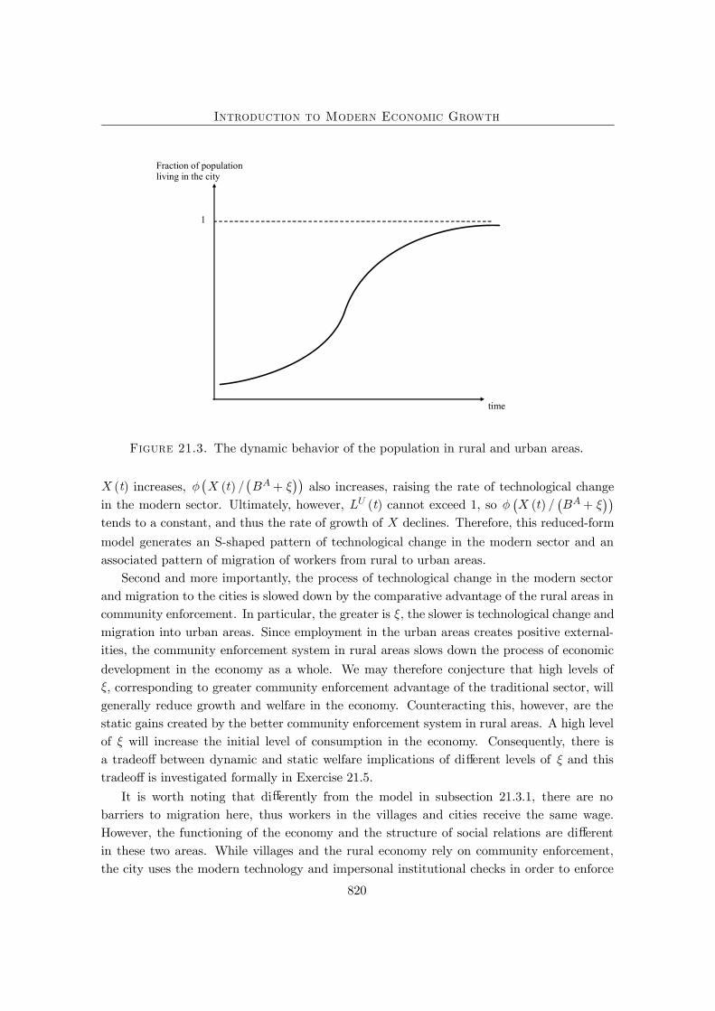
A number of features about this law of motion are worth noting. First, the typical evolu-tion of ( ) will be given as in Figure 21.3, with an S-shaped pattern. This is because startingwith a low initial value of (0), equilibrium in urban employment,
¡( )
¡+¢¢, will
also be low during the early stages of development. This implies that there will be limitedlearning-by-doing and the modern sector technology will progress only slowly. However, as
819
Introduction to Modern Economic Growth
time
1
Fraction of populationliving in the city
Figure 21.3. The dynamic behavior of the population in rural and urban areas.
( ) increases,¡
( )¡
+¢¢also increases, raising the rate of technological change
in the modern sector. Ultimately, however, ( ) cannot exceed 1, so¡( )
¡+¢¢
tends to a constant, and thus the rate of growth of declines. Therefore, this reduced-formmodel generates an S-shaped pattern of technological change in the modern sector and anassociated pattern of migration of workers from rural to urban areas.
Second and more importantly, the process of technological change in the modern sectorand migration to the cities is slowed down by the comparative advantage of the rural areas incommunity enforcement. In particular, the greater is , the slower is technological change andmigration into urban areas. Since employment in the urban areas creates positive external-ities, the community enforcement system in rural areas slows down the process of economicdevelopment in the economy as a whole. We may therefore conjecture that high levels of, corresponding to greater community enforcement advantage of the traditional sector, willgenerally reduce growth and welfare in the economy. Counteracting this, however, are thestatic gains created by the better community enforcement system in rural areas. A high levelof will increase the initial level of consumption in the economy. Consequently, there isa tradeo between dynamic and static welfare implications of di erent levels of and thistradeo is investigated formally in Exercise 21.5.
It is worth noting that di erently from the model in subsection 21.3.1, there are nobarriers to migration here, thus workers in the villages and cities receive the same wage.However, the functioning of the economy and the structure of social relations are di erentin these two areas. While villages and the rural economy rely on community enforcement,the city uses the modern technology and impersonal institutional checks in order to enforce
820
Introduction to Modern Economic Growth
various economic and social arrangements. Consequently, the dual economy in this modelexhibits itself as much in the social dimension as in the economic dimension.
21.3.3. Inappropriate Technologies and the Dual Economy. I now discuss howideas related to appropriate and inappropriate technologies presented in Chapter 18 mayprovide promising clues about other important aspects of the dual economy. Recall from Sec-tion 18.4 that less-developed economies often import their technologies from more advancedeconomies and that these technologies are typically designed for di erent factor proportionsthan those of the less-developed economy. For example, in Section 18.4, I emphasized theimplications of a potential mismatch between the skills of the workforce of a less-developedeconomy and the skill requirements of modern technologies. However, in that model theequilibrium always involved all workers in the less-developed economy using the moderntechnology.
Here suppose that each technology is of the Leontief type, so that it requires a certainnumber of skilled and unskilled workers. For example, technology will produce a totalof units of the unique Þnal good, where is the number of unskilled workers, but thistechnology requires a ratio of skilled to unskilled workers exactly equal to (for example,the skilled workers will be the managers of the unskilled workers). Suppose is increasingin , so that more advanced technologies are more productive.
Now consider a less-developed economy that has access to all technologies for£0 ¯¤
for some ¯ . Suppose that the population of this economy consists of skilled andunskilled workers, such that ¯. This inequality implies that not all workers can beemployed with the most skill-intensive technology. What will the form of equilibrium be inthis economy?
To answer this question, imagine that all markets are competitive, so that the allocation ofworkers to tasks will simply maximize output (recall the Second Welfare Theorem, Theorem5.7). Then, the problem can be written as
(21.31) max[ ( )] [0 ¯]
Z ¯
0( )
subject toZ ¯
0( ) = and ( ) =
where ( ) is the number of unskilled workers assigned to work with technology . TheÞrst-order conditions for this maximization problem can be written as
(21.32) + for all£0 ¯¤
where is the multiplier associated with the Þrst constraint and is the multiplier asso-ciated with the second constraint. The Þrst-order condition is written as an inequality, sincenot all technologies
£0 ¯¤will be used, and those that are not active might satisfy this
condition with a strict inequality.
821
Introduction to Modern Economic Growth
Inspection of the Þrst-order conditions implies that if ¯ is su ciently high and if 0 0,the solution to this problem will have a simple feature. All skilled workers will be employed attechnology ¯, and together with them, there will be
¡¯¢= ¯ unskilled workers employedwith this technology. The remaining
¡¯¢ workers will be employed with the technology= 0 (see Exercise 21.6). This equilibrium will then have the feature of a dual economy.
Two very di erent technologies will be used for production, one more advanced (modern),and the other corresponding to the least advanced technology that is feasible. This dualeconomy structure emerges because of a non-convexity�to maximize output, it is necessaryto operate the most advanced technology, but this exhausts all of the available skilled workers,implying that unskilled workers must be employed in technologies that do not require skilledinputs. This perspective therefore suggests that a dual economy structure may result fromthe import of technologies that are potentially mismatched with the supply of skills in aneconomy.
Models of dual economy based on this type of appropriate technology ideas have not beeninvestigated in detail, though the literature on appropriate technology, which was discussedin Chapter 18, suggests that they may be important in practice. While this model focuses onthe dual economy aspect in production, one can easily generalize this framework by assumingthat the more advanced technology will be operated in urban areas and with contractualarrangements enforced by modern institutions, while the less advanced technology is operatedin villages or rural areas. Thus models based on appropriate (or inappropriate) technologymay be able to account for the broad patterns related to the dual economy, including ruralto urban migration and changes in social arrangements.
21.4. Distance to the Frontier and Changes in the Organization of Production
In this section, I discuss how the structure of production changes over the process ofdevelopment, and how this might be related both to changes in certain aspects of the internalorganization of the Þrm and to a shift in the �growth strategy� of an economy�here, meaningwhether the engine of growth is innovation or imitation. I illustrate these ideas using a simplemodel based on Acemoglu, Aghion and Zilibotti (2006). Because of space restrictions, I onlyprovide a sketch of the model, mainly focusing on the production side.
Consider an economy that is behind the world technology frontier. There is no needto use country indices, since I focus on a single country, taking the behavior of the worldtechnology frontier as given. Time is discrete and the economy is populated by two-periodlived overlapping generations. Total population is normalized to 1. There is a unique Þnalgood, which is also taken as the numeraire. It is produced competitively using a continuumof machines with a technology similar to those in endogenous growth models in Chapter 14,
(21.33) ( ) =Z 1
0( ) ( )1
where ( ) is the productivity of machine variety at time , ( ) is the amount of thismachine used in the production of the Þnal good at time , and (0 1).
822
Introduction to Modern Economic Growth
Each machine good is produced by a monopolist [0 1] at a unit marginal cost interms of the unique Þnal good. The monopolist faces a competitive fringe of imitators thatcan copy its technology and also produce an identical machine with productivity ( ), butcan only do so at the cost of 1 units of Þnal good. The existence of this competitivefringe forces the monopolist to charge a limit price:
(21.34) ( ) = 1
This limit price conÞguration will be an equilibrium when is not so high that the monopolistcan set the unconstrained monopoly price. The condition for this is
1 (1 )
which I impose throughout. The parameter captures both technological factors and govern-ment regulations regarding competitive policy. A higher corresponds to a less competitivemarket. Given the demand implied by the Þnal goods technology in (21.33) and the equilib-rium limit price in (21.34), equilibrium monopoly proÞts are simply:
(21.35) ( ) = ( )
where( 1) 1 (1 )1
is a measure of the extent of monopoly power. In particular it can be veriÞed that isincreasing in for all 1 (1 ).
In this model, the process of economic development will be driven not by capitalaccumulation�which was the force emphasized in some of the earlier models�but by techno-logical progress, that is, by increases in ( ). Let us assume that each monopolist [0 1]can increase its ( ) by two complementary processes: (i) imitation (adoption of existingtechnologies); and (ii) innovation (discovery of new technologies). The key economic trade-o s in the model arise from the fact that di erent economic arrangements (both in terms ofthe organization of Þrms and in terms of the growth strategy of the economy) will lead todi erent amounts of imitation and innovation.
To prepare for this point, let us deÞne the average productivity of the economy in questionat date as:
( )Z 1
0( )
Let ¯ ( ) denote the productivity at the world technology frontier. The fact that this econ-omy is behind the world technology frontier means that ( ) ¯ ( ) for all . The worldtechnology frontier progresses according to the di erence equation
(21.36) ¯ ( ) = (1 + ) ¯ ( 1)
where the growth rate of the world technology frontier is taken to be
(21.37) + ¯ 1
where and ¯ will be deÞned below.
823
Introduction to Modern Economic Growth
I assume that the process of imitation and innovation leads to the following law of motionof each monopolist�s productivity:
(21.38) ( ) = ¯ ( 1) + ( 1) + ( )
where 0 and 0, and ( ) is a random variable with zero mean, capturing di erencesin innovation performance across Þrms and sectors.
In equation (21.38), ¯ ( 1) stands for advances in productivity coming from adoptionof technologies from the frontier (and thus depends on the productivity level of the frontier,¯( 1)), while ( 1) stands for the component of productivity growth coming frominnovation (building on the existing knowledge stock of the economy in question at time
1, ( 1)). Let us also deÞne
( )( )¯ ( )
as the (inverse) measure of the country�s distance to the technological frontier at date .Now, integrate (21.38) over [0 1], use the fact that ( ) has mean zero, divide
both sides by ¯ ( ) and use (21.36) to obtain a simple linear relationship between a country�sdistance to frontier ( ) at date and the distance to frontier ( 1) at date 1:
(21.39) ( ) =1
1 +( + ( 1))
This equation is similar to the technological catch-up equation in Section 18.2 in Chapter18. It shows how the dual process of imitation and innovation may lead to a process ofconvergence. In particular, as long as 1 + , equation (21.39) implies that ( ) willeventually converge to 1. Second, the equation also shows that the relative importance ofimitation and innovation depends on the distance to the frontier of the economy in question.In particular when ( ) is large (meaning the country is close to the frontier), innovation,, matters more for growth. In contrast when ( ) is small (meaning the country is fartherfrom the frontier), imitation, , is relatively more important.
To obtain further insights, let us now endogenize and using a reduced-form approach.Following the analysis in Acemoglu, Aghion and Zilibotti (2006), I model the parametersand as functions of the investments undertaken by the entrepreneurs and the contractualarrangement between Þrms and entrepreneurs. The key idea is that there are two types ofentrepreneurs: high-skill and low-skill. When an entrepreneur starts a business, his skilllevel is unknown and is revealed over time through his subsequent performance. This impliesthat there are two types of �growth strategies� that are possible. The Þrst one emphasizesselection of high-skill entrepreneurs and will replace any entrepreneur that is revealed to below skill. This growth strategy will involve a high degree of churning (creative destruction)and a large number of young entrepreneurs (as older unsuccessful entrepreneurs are replacedby new young entrepreneurs). The second strategy maintains experienced entrepreneurs inplace even when they have low skills. This strategy therefore involves an organization of Þrmsrelying on �longer-term relationships� (here between entrepreneurs and the credit market),an emphasis on experience and cumulative earnings, and less creative destruction. While
824
Introduction to Modern Economic Growth
low-skill entrepreneurs are less productive than high-skill entrepreneurs, there are potentialreasons for why an experienced low-skill entrepreneur might be preferred to a new youngentrepreneur. For example, experience may increase productivity, at least in certain tasks.Alternatively, Acemoglu, Aghion and Zilibotti (2006) show that in the presence of creditmarket imperfections, the retained earnings of an old entrepreneur may provide him with anadvantage in the credit market (because he can leverage his existing earnings to raise moremoney and undertake greater productivity-enhancing investments). I denote the strategybased on selection by = 0, while the strategy that maintains experienced entrepreneurs inplace is denoted by = 1.
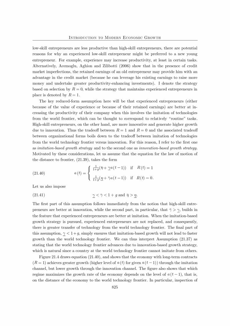
The key reduced-form assumption here will be that experienced entrepreneurs (eitherbecause of the value of experience or because of their retained earnings) are better at in-creasing the productivity of their company when this involves the imitation of technologiesfrom the world frontier, which can be thought to correspond to relatively �routine� tasks.High-skill entrepreneurs, on the other hand, are more innovative and generate higher growthdue to innovation. Thus the tradeo between = 1 and = 0 and the associated tradeobetween organizational forms boils down to the tradeo between imitation of technologiesfrom the world technology frontier versus innovation. For this reason, I refer to the Þrst oneas imitation-based growth strategy and to the second one as innovation-based growth strategy.Motivated by these considerations, let us assume that the equation for the law of motion ofthe distance to frontier, (21.39), takes the form
(21.40) ( ) =
11+ (¯ + ( 1)) if ( ) = 1
11+ ( + ¯ ( 1)) if ( ) = 0
Let us also impose
(21.41) ¯ 1 + and ¯
The Þrst part of this assumption follows immediately from the notion that high-skill entre-preneurs are better at innovation, while the second part, in particular, that ¯ , builds inthe feature that experienced entrepreneurs are better at imitation. When the imitation-basedgrowth strategy is pursued, experienced entrepreneurs are not replaced, and consequently,there is greater transfer of technology from the world technology frontier. The Þnal part ofthis assumption, 1+ , simply ensures that imitation-based growth will not lead to fastergrowth than the world technology frontier. We can thus interpret Assumption (21.37) asstating that the world technology frontier advances due to innovation-based growth strategy,which is natural since a country at the world technology frontier cannot imitate from others.
Figure 21.4 draws equation (21.40), and shows that the economy with long-term contracts( = 1) achieves greater growth (higher level of ( ) for given ( 1)) through the imitationchannel, but lower growth through the innovation channel. The Þgure also shows that whichregime maximizes the growth rate of the economy depends on the level of ( 1), that is,on the distance of the economy to the world technology frontier. In particular, inspection of
825
Introduction to Modern Economic Growth
45º
a(t)1
a(t+1)
â
R = 1
R = 0
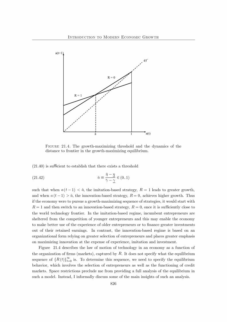
Figure 21.4. The growth-maximizing threshold and the dynamics of thedistance to frontier in the growth-maximizing equilibrium.
(21.40) is su cient to establish that there exists a threshold
(21.42) �¯¯
(0 1)
such that when ( 1) �, the imitation-based strategy, = 1 leads to greater growth,and when ( 1) �, the innovation-based strategy, = 0, achieves higher growth. Thusif the economy were to pursue a growth-maximizing sequence of strategies, it would start with= 1 and then switch to an innovation-based strategy, = 0, once it is su ciently close to
the world technology frontier. In the imitation-based regime, incumbent entrepreneurs aresheltered from the competition of younger entrepreneurs and this may enable the economyto make better use of the experience of older entrepreneurs or to Þnance greater investmentsout of their retained earnings. In contrast, the innovation-based regime is based on anorganizational form relying on greater selection of entrepreneurs and places greater emphasison maximizing innovation at the expense of experience, imitation and investment.
Figure 21.4 describes the law of motion of technology in an economy as a function ofthe organization of Þrms (markets), captured by . It does not specify what the equilibriumsequence of { ( )} =0 is. To determine this sequence, we need to specify the equilibriumbehavior, which involves the selection of entrepreneurs as well as the functioning of creditmarkets. Space restrictions preclude me from providing a full analysis of the equilibrium insuch a model. Instead, I informally discuss some of the main insights of such an analysis.
826
Introduction to Modern Economic Growth
Conceptually, one might want to distinguish among four conÞgurations, which arise asequilibria under di erent institutional settings and parameter values.
1. Growth-maximizing equilibrium : the Þrst and the most obvious possibility is an equi-librium that is growth maximizing. In particular, if markets and entrepreneurs have growthmaximization as their objective and are able to solve the agency problems, have the rightdecision-making horizon and are able to internalize the pecuniary and non-pecuniary exter-nalities, we would obtain an e cient equilibrium. This equilibrium will take a simple form:
( ) =1 if ( 1) �
0 if ( 1) �
so that the economy achieves the upper envelope of the two lines in Figure 21.4. In thiscase, there is no possibility of outside intervention to increase the growth rate of the econ-omy.2 Moreover, an economy starting with (0) 1 always achieves a growth rate greaterthan , and will ultimately converge to the world technology frontier, that is, ( ) 1. Inthis growth-maximizing equilibrium, the economy Þrst starts with a particular set of orga-nizations/institutions, corresponding to = 1. Then, the economy undergoes a structuraltransformation�in this case, a change in its organizational form�switching from = 1to = 0. In our simple economy, this structural transformation takes the form of long-term relationships disappearing and being replaced by shorter-term relationships, by greatercompetition among entrepreneurs and Þrms and by better selection of entrepreneurs.
2. Underinvestment equilibrium: the second potential equilibrium conÞguration involvesthe following equilibrium organizational form:
( ) =1 if ( 1) ( )
0 if ( 1) ( )
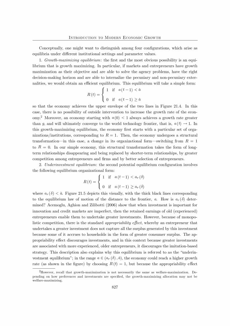
where ( ) �. Figure 21.5 depicts this visually, with the thick black lines correspondingto the equilibrium law of motion of the distance to the frontier, . How is ( ) deter-mined? Acemoglu, Aghion and Zilibotti (2006) show that when investment is important forinnovation and credit markets are imperfect, then the retained earnings of old (experienced)entrepreneurs enable them to undertake greater investments. However, because of monopo-listic competition, there is the standard appropriability e ect, whereby an entrepreneur thatundertakes a greater investment does not capture all the surplus generated by this investmentbecause some of it accrues to households in the form of greater consumer surplus. The ap-propriability e ect discourages investments, and in this context because greater investmentsare associated with more experienced, older entrepreneurs, it discourages the imitation-basedstrategy. This description also explains why this equilibrium is referred to as the �underin-vestment equilibrium�; in the range ( ( ) �), the economy could reach a higher growthrate (as shown in the Þgure) by choosing ( ) = 1, but because the appropriability e ect
2However, recall that growth-maximization is not necessarily the same as welfare-maximization. De-pending on how preferences and investments are speciÞed, the growth-maximizing allocation may not bewelfare-maximizing.
827
Introduction to Modern Economic Growth
45º
a(t)1
a(t+1)
â
R = 1
R = 0
ar( )
Figure 21.5. Dynamics of the distance to frontier in the underinvestment equilibrium.
discourages investments, there is a switch to the innovation-based equilibrium earlier thanthe growth-maximizing threshold.
A notable feature is that although the equilibrium is di erent from the previous case, itagain starts with = 1 and is followed by a structural transformation, that is, by a switch tothe innovation-based regime ( = 0). Moreover, the economy still ultimately converges to theworld technology frontier, that is, ( ) = 1 is reached as . The only di erence is thatthe structural transformation from = 1 to = 0 happens too soon, at ( 1) = ( ),rather than at the growth-maximizing threshold �.
Consequently, in this case, a temporary government intervention may increase the growthrate of the economy. The temporary aspect is important here, since the best that the gov-ernment can do is to increase the growth rate while ( ( ) �). How can the governmentachieve this? Subsidies to investment would be one possibility. Acemoglu, Aghion and Zili-botti (2006) show that the degree of competition in the product market also has an indirecte ect on the equilibrium, as emphasized by the notation ( ). In particular, a higher levelof , which corresponds to lower competition in the product market (higher ), will increase( ), and thus may close the gap between ( ) and �. Nevertheless, it has to be noted
that reducing competition will create other, static distortions (because of higher markups).Moreover and more importantly, we will see in the next two conÞgurations that reducingcompetition can have much more detrimental e ects on economic growth, so any use ofcompetition policy for this purpose must be subject to serious caveats.
828
Introduction to Modern Economic Growth
45º
a(t)1
a(t+1)
â
R = 1
R = 0
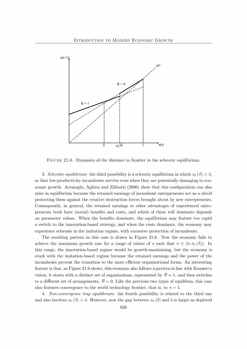
ar( )
Figure 21.6. Dynamics of the distance to frontier in the sclerotic equilibrium.
3. Sclerotic equilibrium: the third possibility is a sclerotic equilibrium in which ( ) �,so that low-productivity incumbents survive even when they are potentially damaging to eco-nomic growth. Acemoglu, Aghion and Zilibotti (2006) show that this conÞguration can alsoarise in equilibrium because the retained earnings of incumbent entrepreneurs act as a shieldprotecting them against the creative destruction forces brought about by new entrepreneurs.Consequently, in general, the retained earnings or other advantages of experienced entre-preneurs both have (social) beneÞts and costs, and which of these will dominate dependson parameter values. When the beneÞts dominate, the equilibrium may feature too rapida switch to the innovation-based strategy, and when the costs dominate, the economy mayexperience sclerosis in the imitation regime, with excessive protection of incumbents.
The resulting pattern in this case is drawn in Figure 21.6. Now the economy fails toachieve the maximum growth rate for a range of values of such that (� ( )). Inthis range, the innovation-based regime would be growth-maximizing, but the economy isstuck with the imitation-based regime because the retained earnings and the power of theincumbents prevent the transition to the more e cient organizational forms. An interestingfeature is that, as Figure 21.6 shows, this economy also follows apattern in line with Kuznets�svision; it starts with a distinct set of organizations, represented by = 1, and then switchesto a di erent set of arrangements, = 0. Like the previous two types of equilibria, this casealso features convergence to the world technology frontier, that is, to = 1.
4. Non-convergence trap equilibrium: the fourth possibility is related to the third oneand also involves ( ) �. However, now the gap between ( ) and � is larger as depicted
829
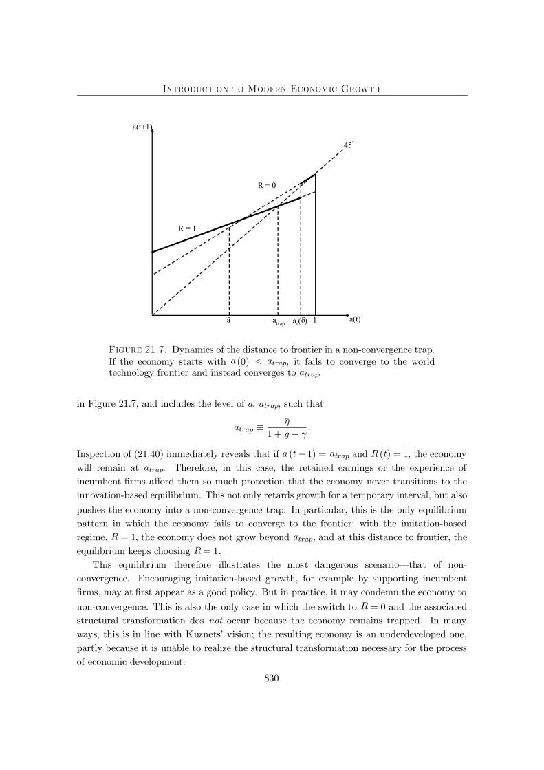
Introduction to Modern Economic Growth
45º
a(t)1
a(t+1)
â
R = 1
R = 0
ar( )atrap
Figure 21.7. Dynamics of the distance to frontier in a non-convergence trap.If the economy starts with (0) , it fails to converge to the worldtechnology frontier and instead converges to .
in Figure 21.7, and includes the level of , , such that
¯1 +
Inspection of (21.40) immediately reveals that if ( 1) = and ( ) = 1, the economywill remain at . Therefore, in this case, the retained earnings or the experience ofincumbent Þrms a ord them so much protection that the economy never transitions to theinnovation-based equilibrium. This not only retards growth for a temporary interval, but alsopushes the economy into a non-convergence trap. In particular, this is the only equilibriumpattern in which the economy fails to converge to the frontier; with the imitation-basedregime, = 1, the economy does not grow beyond , and at this distance to frontier, theequilibrium keeps choosing = 1.
This equilibrium therefore illustrates the most dangerous scenario�that of non-convergence. Encouraging imitation-based growth, for example by supporting incumbentÞrms, may at Þrst appear as a good policy. But in practice, it may condemn the economy tonon-convergence. This is also the only case in which the switch to = 0 and the associatedstructural transformation dos not occur because the economy remains trapped. In manyways, this is in line with Kuznets� vision; the resulting economy is an underdeveloped one,partly because it is unable to realize the structural transformation necessary for the processof economic development.
830

Introduction to Modern Economic Growth
Taken together the four scenarios suggest that depending on the details of the model,there should be no presumption that the e cient or the growth-maximizing sequence ofgrowth strategies will be pursued. Thus, some degree of government intervention might beuseful. However, the third and the fourth cases also emphasize that government interventioncan have negative unintended consequences. It may improve growth during a limited periodof time (in the second scenario this will be when ( ( ) �)), but it may subsequentlycreate much more substantial costs by leading to a non-convergence trap as shown in Figure21.7.
Even though the implications of these four scenarios for government intervention aremixed, their implications for changes in the structure of organizations over the developmentprocess are clearer; regardless of which scenario applies, the economy starts with a distinctorganization of production, where longer-term contracts, incumbent producers, experienceand imitation are more important, and then, except in the non-convergence trap equilibrium,it ultimately switches to an equilibrium with greater creative destruction, shorter-term rela-tionships, younger entrepreneurs and more innovation. This is another facet of the structuraltransformations emphasized by Kuznets as part of the process of economic development. Theframework presented here, though reduced-form, can also be used to study other aspects ofchanges in the organization of production over the process of development (see Exercise 21.7).
21.5. Multiple Equilibria From Aggregate Demand Externalities and the BigPush
I now present a simple model of multiple equilibria arising from aggregate demand ex-ternalities, based on Murphy, Shleifer and Vishny�s (1989) �big push� model. This modelformalizes ideas Þrst proposed by Rosenstein-Rodan (1943), Hirschman (1958) and Nurske(1958), that economic development can (or should) be viewed as a move from one (Paretoine cient) equilibrium to another, more e cient equilibrium. Moreover, these early de-velopment economists argued that this type of move requires coordination among di erentindividuals and Þrms in the economy, thus a big push. As already discussed in Chapter 4,multiple equilibria, literally interpreted, are unlikely to be the root cause of persistently lowlevels of development, since if there is indeed a Pareto improvement�a change that will makeall individuals better-o �it is unlikely that the necessary coordination cannot be achievedfor decades or even centuries. Nevertheless, the forces leading to multiple equilibria highlightimportant economic mechanisms that can be associated with market failures slowing down,or even preventing, the process of development. Moreover, dynamic versions of models ofmultiple equilibria can lead to multiple state states, whereby once an economy ends up in asteady state with low economic activity, it may get stuck there (and there is no possibilityof a coordination to jump to the other steady state). Models with multiple steady states,which are more useful for thinking about the process of long-run development than modelswith multiple equilibria, will be discussed in the next section.
831
Introduction to Modern Economic Growth
Murphy, Shleifer and Vishny formalize the ideas related to the big push using a modelwith multiple equilibria due to aggregate demand externalities. The economy has two periods,= 1 and 2, and admits a representative household with preferences
( (1) (2)) =(1)1 11
+(2)1 11
where (1) and (2) denote consumption at the two dates; is the discount factor ofthe households; and plays a similar role to before; 1 is the intertemporal elasticity ofsubstitution and determines how willing individuals are to substitute consumption betweendate 1 and date 2. The representative household supplies labor inelastically and the totallabor supply is denoted by .
The resource constraints are
(21.43) (1) + (1) (1) and (2) (2)
where (1) denotes investment in the Þrst date, ( ) is total output at date , and investmentis only possible in the Þrst date.
Households can borrow and lend, so their budget constraint can be represented as
(1) +(2)
1 +(1) + (1) +
(2) + (2)1 +
where ( ) denotes the proÞts accruing to the representative household, and ( ) is the wagerate at time . is the interest rate between periods 1 and 2 and will adjust in equilibriumso that the aggregate the resource constraints, (21.43), hold.
The Þnal good is produced from a CES aggregate of di erentiated intermediate goods,with production function
( ) =µZ 1
0( )
1
1
where ( ) is the output level of intermediate at date . As usual is the elasticity ofsubstitution between intermediate goods and we assume that 1.
The production functions of intermediate goods in the two periods are as follows:
( 1) = ( 1)
(21.44) ( 2) =½
( 2) with old technology( 2) with new technology
where 1 and ( ) denotes labor devoted to the production of intermediate good attime . Labor market clearing requires
(21.45)Z 1
0( )
At date 1, there is a designated producer for each intermediate, which I also refer toas a �monopolist�. A competitive fringe of Þrms can also enter and produce each goodas productively as the designated producer. At date 1, the designated producer can alsoinvest in the new technology, which costs in terms of the Þnal good. If this investmentis undertaken, this producer�s productivity at date 2 will be higher by a factor 1 as
832
Introduction to Modern Economic Growth
indicated by equation (21.44). In contrast, the fringe will not beneÞt from this technologicalimprovement, thus the designated producer will have some degree of monopoly power. TheproÞts from intermediate producers are naturally allocated to the representative household.
We will look for the pure-strategy symmetric Subgame Perfect Equilibria (SSPE) of thistwo-period economy (see, for example, Section 18.5 in Chapter 18). SSPE is deÞned inthe usual fashion, as a combination of production and investment decisions for Þrms andconsumption decisions for households that are best responses to each other in both periods.
First, since all goods are symmetric, the Þrst period labor market clearing is straightfor-ward and requires
( 1) = for all [0 1]
(recall that the measure of sectors and Þrms is normalized to 1). This implies that
(1) =
At date 2, the equilibrium will depend on how many Þrms have adopted the new technology.Since the focus is on SSPE, it is su cient to consider the two extreme allocations, whereall Þrms adopt the new technology and where no Þrm adopts. In either case, the marginalproductivity of all sectors is the same, so labor will be allocated equally so that
( 2) = for all [0 1]
Consequently, when the technology is not adopted,
(2) =
and when the technology is adopted by all the Þrms,
(2) =
I now turn to the pricing decisions. In the Þrst date, the designated producers have nomonopoly power because of the competitive fringe, thus they charge price equal to marginalcost, which is (1), and they make zero proÞts. Since total output is equal to (1) = , thisalso implies that the equilibrium wage rate is (1) = 1. In the second date, if the technologyis not adopted, the equilibrium is identical to that at date 1, so (2) = 1, and thus there willbe no proÞts. In this case there is also no investment, so consumption at both dates is equalto . Since the consumption Euler equation is (1) = (1 + ) (2) , the equilibriuminterest rate in this case is
(21.46) �= 1 1.
Next consider the situation in which the designated producers have invested in the ad-vanced technology. Now they can produce units of output with one unit of labor, while thefringe of competitive Þrms still produces one unit of output with one unit of labor. This im-plies that the designated producers have some monopoly power. The extent of this monopolypower depends on the comparison of and .
833
Introduction to Modern Economic Growth
Let us Þrst determine the demand facing each producer, which is given as a solution tothe following program of proÞt maximization for the Þnal good sector:
max[ ( 2)] [0 1]
Z 1
0( 2)
1¸
1Z 1
0( 2) ( 2)
where ( 2) is the price of intermediate at date 2. The Þrst-order condition to thisprogram implies
(21.47) ( 2) = ( 2) (2)
This expression is useful in laying the foundations for the aggregate demand externalities; thedemand for intermediate depends on the total amount of production, (2). The familiarfeature of the demand curve (21.47) is that it is isoelastic. To make further progress, Þrstimagine the situation in which there is no fringe of competitive producers. In that case, eachdesignated producer will act as an unconstrained monopolist and maximize its proÞts givenby price minus marginal cost times quantity, that is,
( 2) =µ( 2)
(2)
( 2)
Substituting from (21.47), the Þrm maximization problem is thus
max( 2)
µ( 2)
(2)¶( 2) (2)
which gives the proÞt-maximizing price as
( 2) =1
(2)
This is the standard monopoly price formula with a markup related to demand elasticity overthe marginal cost. The markup is constant because the demand elasticity is constant.
However, the monopolist can only charge this price if the competitive fringe cannot en-ter and make proÞts stealing the entire market at this price. Since the competitive fringecan produce one unit using one unit of labor, the monopolist can only charge this price if(( 1) ) 1. Otherwise, the price would be too high and the competitive fringe would
enter. Let us assume that is not so high as to make the monopolist unconstrained. In otherwords, let us assume
(21.48)11
1
Under this assumption, the monopolist will be forced to charge a limit price. It is straight-forward to see that this equilibrium limit price would be = (2). Consequently, given(21.48), each monopolist would make per unit proÞts equal to
(2)(2)
=1(2)
Total proÞts are then obtained from (21.47) as
(21.49) (2) =1(2)1 (2)
834
Introduction to Modern Economic Growth
The wage rate can be determined from income accounting. Total production will be equalto (2) = , and this has to be distributed between proÞts and wages, thus
1(2)1 + (2) =
which has a solution of (2) = 1, exactly the same as in the case without the technologicalinvestments. Intuitively, wages in this economy are determined by the demand from thecompetitive fringe and thus the greater marginal product does not directly beneÞt workers.Instead, it increases monopolists� proÞts. Nevertheless, all of these proÞts are redistributedto households, who are the owners of the Þrms. Thus (2) = . However, because ofinvestment in the new technology at date 1, (1) = . The consumption Euler equationnow requires ( ) = (1 + �) ( ) , which gives the equilibrium interest-rate in thiscase as
�= 1µ 
1 �
where � is given by (21.46). The interest rate in this case, �, is higher than � becauseindividuals are now being asked to forgo date 1 consumption for date 2 consumption. Notealso that the greater is , the higher is �, since with a greater , there is less intertemporalsubstitution. Also a higher , meaning a greater consumption sacriÞce at date 1, implies ahigher interest rate.
The question is whether a monopolist will Þnd it proÞtable to undertake the investmentat date 1. The reason for the possibility of multiplicity of equilibria is that the answer to thisquestion will depend on whether other Þrms are undertaking the investment or not. Let usÞrst consider a situation in which no other Þrm is undertaking the investment, and considerthe incentives of a single monopolist to undertake such an investment.
In this case total output at date 2 is equal to (since the Þrm considering investmentis inÞnitesimal), and the market interest rate is given by �. Moreover, from (21.49) and thefact that (2) = 1, proÞts at date 2 are
(2) =1
where the superscript denotes that no other Þrm is undertaking the investment. Therefore,the net discounted proÞts at date 1 for the Þrm in question are
= +11+ �
1= +
1
Next consider the case in which all other Þrms are undertaking the investment. In thiscase, proÞts at date 2 are
(2) = ( 1)
where the superscript designates that all other Þrms are undertaking the investment. Con-sequently, the proÞt gain from investing at date 1 is
= +11 + �
( 1) = +µ 
( 1)
835
Introduction to Modern Economic Growth
As discussed above, the idea of the paper by Murphy, Shleifer and Vishny (1989), sim-ilar to the ideas of many economists writing on economic development before them, was togenerate multiple equilibria, with one corresponding to backwardness and the other to in-dustrialization. In this context, this means that for the same parameter values, both theallocations with no investment in the new technology and with all monopolists investing inthe new technology should be equilibria. This is possible if
(21.50) 0 and 0
that is, when nobody else invests, investment is not proÞtable, and when all other Þrms invest,investment is proÞtable. This is clearly possible because the aggregate demand externalitiesensure that ; when other Þrms invest, they produce more, there is greater aggregatedemand, and proÞts from the new technology are higher. Counteracting this e ect is the factthat the interest rate is also higher when all Þrms invest. Therefore, the existence of multipleequilibria requires the interest rate e ect not to be too strong. For example, in the extremecase where preferences are linear ( = 0), we have
= + ( 1) = +1
so the conÞguration in (21.50) is certainly possible. More generally, the condition for theexistence of multiple equilibria is that:
(21.51)µ 
( 1)1
It is also straightforward to see that whenever both equilibria exist, the equilibrium withinvestment Pareto dominates the one without investment, since condition (21.51) implies thatall households are better-o with the upward sloping consumption proÞle giving them higherconsumption at date 2 (see Exercise 21.8). Therefore, this analysis establishes that whencondition (21.51) is satisÞed, there will exist two SSPE. In one of these, all Þrms undertakethe investment at date 1 and households are better-o , while in the other one there are noinvestments in new technology and greater market failures. Intuitively, investing in the newtechnology at date 1 is proÞtable only when there is su cient aggregate demand at date2, and in turn, there will be su cient demand at date 2 when all Þrms invest in the newtechnology. Aggregate demand externalities are responsible for multiple equilibria here. Inparticular, the investment decision of a Þrm creates a positive (pecuniary) externality on otherÞrms by increasing the level of demand facing their products. These pecuniary externalitiescorrespond to �Þrst-order� e ects because of monopoly markups: Þrms do not capture thefull gains from increased production, which instead creates Þrst-order gains for householdsand for other Þrms that can sell more.
The interpretation for this result suggested by Murphy, Shleifer and Vishny is to considerthe equilibrium with no investment in the new technology as representing a �developmenttrap,� where the economy remains in �underdevelopment� because no Þrm undertakes theinvestment in new technology and this behavior implies that the demand necessary to make
836
Introduction to Modern Economic Growth
such investments proÞtable is absent. In contrast, the equilibrium with investment in newtechnology is interpreted as corresponding to �industrialization�. According to this inter-pretation, societies that can somehow coordinate on the equilibrium with investment (eitherbecause private expectations are aligned or because of some type of government action)will industrialize and realize both economic growth and Pareto improvement. As such, thismodel is argued to provide a formalization of the �big push� type industrialization describedby economists such as Nurske or Rosenstein-Rodan. Although the idea of the big push andthe aggregate demand externalities are attractive, the model here su ers from a number ofobvious shortcomings. First, even though the process of industrialization is a dynamic one,the model here is static. Therefore, it does not allow a literal interpretation of a society beingÞrst in the no investment equilibrium and then changing to the investment equilibrium andindustrializing. Second, as already discussed in Chapter 4, models with multiple equilibriado not provide satisfactory theories of development, since it is di cult to imagine a societyremaining unable to coordinate on a simple range of actions that would make all households(and Þrms) better-o . Instead, it is much more likely that the ideas related to aggregatedemand externalities (or other potential forces leading to multiple equilibria) are more im-portant as sources of persistence or as mechanisms generating multiple steady states (whilestill maintaining a unique equilibrium path).
21.6. Inequality, Credit Market Imperfections and Human Capital
The previous section illustrated how aggregate demand externalities can generate devel-opment traps. Investment by di erent Þrms may require coordination, leading to multipleequilibria. Underdevelopment may be thought to correspond to a situation in which thecoordination is on the bad equilibrium, and the development process starts with the �bigpush,� ensuring coordination to the high-investment equilibrium. Here I illustrate a relatedset of issues in the context of the impact of the distribution of income on human capital underimperfect credit markets. In contrast to the previous section, I will emphasize the possibil-ity of multiple steady states (rather than multiple equilibria). In addition, while I focus onhuman capital investments, inequality and credit market problems inßuence not only humancapital investments, but also business creation, occupational choices and other aspects of theorganization of production. Nevertheless, models focusing on the link between inequalityand human capital are both more tractable and also constitute a natural continuation of thetheories of human capital investments presented in Chapter 10.
21.6.1. A Simple Case With No Borrowing. When credit markets are imperfect, amajor determinant of human capital investments will be the distribution of income (as wellas the degree of imperfection in credit markets). I start with a discussion of the simplest casein which there is no borrowing or lending, which introduces an extreme form of credit marketproblems. I then enrich this model by introducing imperfect credit markets, where the costof borrowing is greater than the interest rate received by households engaged in saving.
837
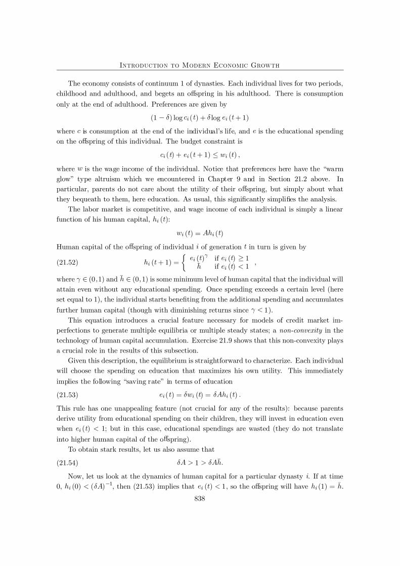
Introduction to Modern Economic Growth
The economy consists of continuum 1 of dynasties. Each individual lives for two periods,childhood and adulthood, and begets an o spring in his adulthood. There is consumptiononly at the end of adulthood. Preferences are given by
(1 ) log ( ) + log ( + 1)
where is consumption at the end of the individual�s life, and is the educational spendingon the o spring of this individual. The budget constraint is
( ) + ( + 1) ( )
where is the wage income of the individual. Notice that preferences here have the �warmglow� type altruism which we encountered in Chapter 9 and in Section 21.2 above. Inparticular, parents do not care about the utility of their o spring, but simply about whatthey bequeath to them, here education. As usual, this signiÞcantly simpliÞes the analysis.
The labor market is competitive, and wage income of each individual is simply a linearfunction of his human capital, ( ):
( ) = ( )
Human capital of the o spring of individual of generation in turn is given by
(21.52) ( + 1) =½
( ) if ( ) 1¯ if ( ) 1
where (0 1) and ¯ (0 1) is some minimum level of human capital that the individual willattain even without any educational spending. Once spending exceeds a certain level (hereset equal to 1), the individual starts beneÞting from the additional spending and accumulatesfurther human capital (though with diminishing returns since 1).
This equation introduces a crucial feature necessary for models of credit market im-perfections to generate multiple equilibria or multiple steady states; a non-convexity in thetechnology of human capital accumulation. Exercise 21.9 shows that this non-convexity playsa crucial role in the results of this subsection.
Given this description, the equilibrium is straightforward to characterize. Each individualwill choose the spending on education that maximizes his own utility. This immediatelyimplies the following �saving rate� in terms of education
(21.53) ( ) = ( ) = ( )
This rule has one unappealing feature (not crucial for any of the results): because parentsderive utility from educational spending on their children, they will invest in education evenwhen ( ) 1; but in this case, educational spendings are wasted (they do not translateinto higher human capital of the o spring).
To obtain stark results, let us also assume that
(21.54) 1 ¯
Now, let us look at the dynamics of human capital for a particular dynasty . If at time0, (0) ( ) 1, then (21.53) implies that ( ) 1, so the o spring will have (1) = ¯.
838
Introduction to Modern Economic Growth
Given (21.54), (1) = ¯ ( ) 1, and repeating this argument, ( ) = ¯ ( ) 1 forall . Therefore, a dynasty that starts with (0) ( ) 1 will never reach a human capitallevel greater than ¯.
45º
hi(t)( A)-1
hi(t+1)
1
h h*
Figure 21.8. Dynamics of human capital with nonconvexities and no borrowing.
Next consider a dynasty with (0) ( ) 1. Then, from (21.54), (1) = ( (0))1, so this dynasty will gradually accumulate more and more human capital over generationsand ultimately reach the �steady state� given by = ( ) or
= ( )1 1
Naturally, this description applies to a dynasty with (0) (( ) 1 ). If (0) ,then the dynasty would have too much human capital and would decumulate human capital.
Figure 21.8 illustrates the dynamics of individual human capital decisions. It shows thatthere are two steady-state levels of human capital for individuals, ¯ and ¯. An importantquestion when there are multiple steady states is where, given initial conditions, the economy(or a particular individual) will converge to. Assume for now that, even though there aremultiple steady states, the equilibrium is unique (meaning that given initial conditions thereis a unique equilibrium path�this will be the case in all the models discussed in this section).Then, equilibrium dynamics are represented by a dynamical system with the only di erencethat there are multiple steady states. Each (locally) asymptotically stable steady state willhave a basin of attraction, meaning a set of initial conditions, which will ultimately lead tothis particular steady state. Both steady states in the model studied here are asymptoticallystable and Figure 21.8 plots their basins of attractions. In particular, inspection of this Þgure
839
Introduction to Modern Economic Growth
shows that dynasties with (0) ( ) 1 will tend to the lower steady state level of humancapital, ¯ , while those with (0) ( ) 1 will tend to the higher level, .
This Þgure also reveals why the dynamics in this model are so simple; the dynamics ofthe human capital of a single individual contain all the information relevant for the dynamicsof the human capital and income of the entire economy. This is because there are no prices(such as the rate of return to human capital or the interest rate) that are determined inequilibrium here. For this reason, dynamics in this type of models are sometimes describedas Markovian�because they are summarized by the Markov process describing the behaviorof the human capital of a single individual (without any general equilibrium interactions).Markovian models are much more tractable than those where dynamics of inequality dependon equilibrium prices. An example of this richer type of model is given in Exercise 21.13.
The most important implication of this analysis is again the presence of poverty traps.This is most clearly illustrated by an economy with two groups starting at income levels
1 and 2 1 such that ( ) 12. Now if inequality (poverty) is high so that 1
( ) 1, a signiÞcant fraction of the population will never accumulate much human capital.In contrast, if inequality is limited so that 1 ( ) 1, all agents will accumulate humancapital, eventually reaching . This example also illustrates that there are (many) multiplesteady states in this economy. Depending on the fraction of dynasties that start with initialhuman capital below ( ) 1, any fraction of the population may end up at the low level ofhuman capital, ¯ . The greater is this fraction, the poorer is the economy.
There are certain parallels between the multiplicity of steady states here and the multipleequilibria highlighted in the model of the previous section. Nevertheless, the di erences arein fact more important. In the model of the previous section, there are multiple equilibria in astatic model. Thus nothing determines which equilibrium the economy will be in. At best, wecan appeal to �expectations,� arguing that the better equilibrium will emerge when everybodyexpects the better equilibrium to emerge. One can informally appeal to the role of �history,�for example, suggesting that if an economy has been in the low investment equilibrium fora while, it is likely to stay there, but this argument is misleading. First of all, the modelis a static one, thus a discussion of an economy �that has been in the low equilibrium for awhile� is not quite meaningful. Secondly, even if the model were turned into a dynamic oneby repeating it over time, the history of being in one equilibrium for a number of periods willhave no e ect on the existence of multiple equilibria at the next period. In particular, eachstatic equilibrium would still remain an equilibrium in the �dynamic� environment, and theeconomy could suddenly jump from one equilibrium to another. This highlights that modelswith multiple equilibria have a degree of indeterminacy that is both theoretically awkwardand empirically di cult to map to reality. Instead, models with multiple steady states avoidthese thorny issues. The equilibrium is unique, but the initial conditions determine wherethe dynamical system will eventually end up. Because the equilibrium is unique, there is noissue of indeterminacy or expectations a ecting the path of the economy. But also, because
840
Introduction to Modern Economic Growth
multiple steady states are possible, the model can be useful for thinking about potentialdevelopment traps.
This model also shows the importance of the distribution of income in an economy withimperfect credit markets (here with no credit markets). In particular, the distribution ofincome a ects which individuals will be unable to invest in human capital accumulation andthus inßuences the long-run income level of the economy. For this reason, models of this sortare sometimes interpreted as implying that an unequal distribution of income will lead to loweroutput (and growth). The above example with two classes seems to support this conclusion.However, this is not a general result and it is important to emphasize that this class of modelsdoes not make speciÞc predictions about the relationship between inequality and growth. Toillustrate this, consider again the same economy with two classes, but now starting with 1
2 ( ) 1. In this case, neither group will accumulate human capital, but redistributingresources away from group 1 to group 2 (thus increasing inequality), so that we push group2 to 2 ( ) 1, would increase human capital accumulation. This is a general feature:in models with non-convexities, there are no unambiguous results about whether greaterinequality is good or bad for economic growth; it depends on whether greater inequalitypushes more people below or above the critical thresholds. Somewhat sharper results canbe obtained about the e ect of inequality on human capital accumulation and developmentunder additional assumptions. Exercise 21.10 presents a parameterization of inequality in themodel here, which delivers the results that greater inequality leads to lower human capitaland lower output per capita in relatively rich economies, but to greater investments in humancapital in poorer economies.
21.6.2. Human Capital Investments with Imperfect Credit Markets. I nowenrich the environment in the previous subsection by introducing credit markets followingGalor and Zeira�s (1993) model. Each individual still lives for two periods. In his youth, hecan either work or acquire education. The utility function of each individual is
(1 ) log ( ) + log ( )
where again denotes consumption at the end of the life of the individual. The budgetconstraint is
( ) + ( ) ( )
where ( ) is individual �s income at time . Note that preferences still take the �warmglow� form, but the utility of the parent now depends on monetary bequest to the o springrather than the level of education expenditures. It will now be the individuals themselveswho will use the monetary bequests to invest in education. Also, the logarithmic formulationonce again ensures a constant saving rate equal to .
Education is a binary outcome, and educated (skilled) workers earn wage while un-educated workers earn . The required education expenditure to become skilled is , andworkers acquiring education do not earn the unskilled wage, , during the Þrst period of their
841
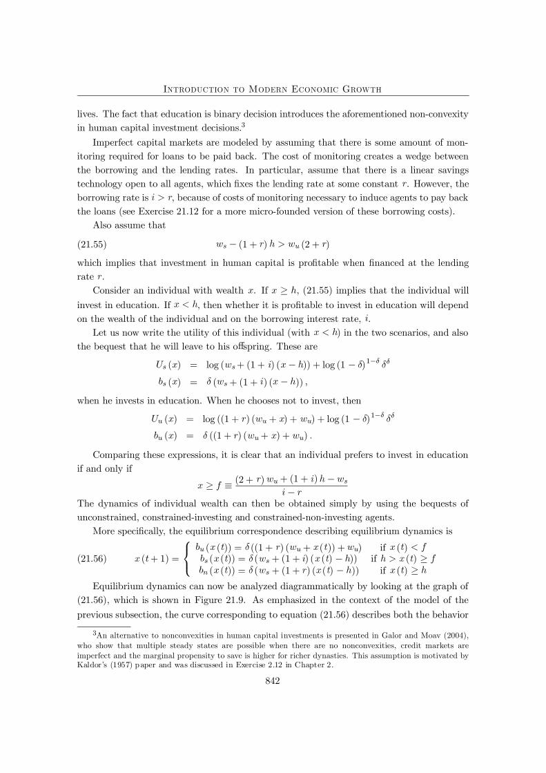
Introduction to Modern Economic Growth
lives. The fact that education is binary decision introduces the aforementioned non-convexityin human capital investment decisions.3
Imperfect capital markets are modeled by assuming that there is some amount of mon-itoring required for loans to be paid back. The cost of monitoring creates a wedge betweenthe borrowing and the lending rates. In particular, assume that there is a linear savingstechnology open to all agents, which Þxes the lending rate at some constant . However, theborrowing rate is , because of costs of monitoring necessary to induce agents to pay backthe loans (see Exercise 21.12 for a more micro-founded version of these borrowing costs).
Also assume that
(21.55) (1 + ) (2 + )
which implies that investment in human capital is proÞtable when Þnanced at the lendingrate .
Consider an individual with wealth . If , (21.55) implies that the individual willinvest in education. If , then whether it is proÞtable to invest in education will dependon the wealth of the individual and on the borrowing interest rate, .
Let us now write the utility of this individual (with ) in the two scenarios, and alsothe bequest that he will leave to his o spring. These are
( ) = log ( + (1 + ) ( )) + log (1 )1
( ) = ( + (1 + ) ( ))
when he invests in education. When he chooses not to invest, then
( ) = log ((1 + ) ( + ) + ) + log (1 )1
( ) = ((1 + ) ( + ) + )
Comparing these expressions, it is clear that an individual prefers to invest in educationif and only if
(2 + ) + (1 + )
The dynamics of individual wealth can then be obtained simply by using the bequests ofunconstrained, constrained-investing and constrained-non-investing agents.
More speciÞcally, the equilibrium correspondence describing equilibrium dynamics is
(21.56) ( + 1) =( ( )) = ((1 + ) ( + ( )) + ) if ( )( ( )) = ( + (1 + ) ( ( ) )) if ( )( ( )) = ( + (1 + ) ( ( ) )) if ( )
Equilibrium dynamics can now be analyzed diagrammatically by looking at the graph of(21.56), which is shown in Figure 21.9. As emphasized in the context of the model of theprevious subsection, the curve corresponding to equation (21.56) describes both the behavior
3An alternative to nonconvexities in human capital investments is presented in Galor and Moav (2004),who show that multiple steady states are possible when there are no nonconvexities, credit markets areimperfect and the marginal propensity to save is higher for richer dynasties. This assumption is motivated byKaldor�s (1957) paper and was discussed in Exercise 2.12 in Chapter 2.
842
Introduction to Modern Economic Growth
of the wealth of each individual and the behavior of the wealth distribution in the aggregateeconomy. This is again a feature of the �Markovian� nature of the current model.
Now deÞne as the intersection of the equilibrium curve (21.56) with the 45 degree linewhen the equilibrium correspondence is steeper. Such an intersection will exist when theborrowing interest rate, , is large enough. Suppose this is the case. Then, Figure 21.9 makesit clear that there will be three intersections between (21.56) and the 45 degree line, ¯ ,and ¯ . Moreover, the Þgure shows that corresponds to an unstable steady state, whilethe other two are locally asymptotically stable.
Figure 21.9. Multiple steady-state equilibria in the Galor and Zeira model.
The basis of attraction of the steady states for ¯ and ¯ are also easy to obtain fromthis Þgure. In particular, all individuals with ( ) converge to the wealth level ¯ ,while all those with ( ) converge to the greater wealth level ¯ . Thus the basinof attraction of ¯ is [0 ], and this corresponds to a �poverty trap,� in the sense thatindividuals (dynasties) with initial wealth in this interval will converge to ¯ . The initialdistribution of income again has a Þrst-order e ect on the e ciency and income level ofthe economy. If the majority of the individuals start with ( ) , the economy willhave low productivity, low human capital and low wealth. Therefore, this model extendsthe insights of the simple model with no borrowing from the previous subsection to a richerenvironment in which individuals make forward-looking human capital investments. The keyis again the interaction between credit market imperfections (which here make the interestrate for borrowing greater than the interest rate for saving) and inequality. As in the modelof the previous subsection, it is straightforward to construct examples where an increase in
843
Introduction to Modern Economic Growth
inequality can lead to either worse or better outcomes depending on whether it pushes moreindividuals into the basin of attraction of the low steady state.
An important feature of the model of this subsection is that because it allows individualsto borrow and lend in Þnancial markets, it enables an investigation of the implications ofÞnancial development for human capital investments. In an economy with better Þnancialinstitutions, the wedge between the borrowing rate and the lending rate will be smaller, thatis, will be smaller for a given level of . With a smaller , more agents will escape the povertytrap, and in fact, the poverty trap may not exist at all (there may not be an intersectionbetween (21.56) and the 45 degree line where (21.56) is steeper). This shows that Þnancialdevelopment not only improves risk sharing as demonstrated in Section 21.1, but in addition,by relaxing credit market constraints, it contributes to human capital accumulation.
Although the model in this section is considerably richer than that in the previous sub-section, it is still a partial equilibrium model. Multiple steady states are possible for di erentindividuals as a function of their initial level of human capital (or wealth), but individual dy-namics are not a ected by general equilibrium prices. Galor and Zeira (1993), Banerjee andNewman (1994), Aghion and Bolton (1997) and Piketty (1997) consider richer environmentsin which income dynamics of each dynasty (individual) are a ected by general equilibriumprices (such as the interest rate or the wage rate), which are themselves a function of the in-come inequality. Exercise 21.11 shows that the type of multiple steady states generated by themodel presented here may not be robust to the addition of noise in income dynamics�insteadof multiple steady states, the long-run equilibrium may generate a stationary distribution ofhuman capital levels, though this stationary distribution would exhibit a large amount ofpersistence.4 In contrast, models in which prices are determined in general equilibrium anda ect wealth (income) dynamics can generate more �robust� multiplicity of steady states.
21.7. Towards a UniÞed Theory of Development and Growth?
There has been a uniÞed theme to the models discussed in this chapter. They have eitheremphasized the transformation of the economy and the society over the process of develop-ment or potential reasons for why such a transformation might be halted. This transformationtakes the form of the structure of production changing, the process of industrialization gettingunderway, a greater fraction of the population migrating from rural areas to cities, Þnancialmarkets becoming more developed, mortality and fertility rates changing via health improve-ments and the demographic transition, and the extent of ine ciencies and market failuresbecoming less pronounced over time. In many instances, the driving force for this process isreinforced by the structural transformation that it causes.
4The reader will note that this is related to the �Markovian� nature of the model. Markovian models cangenerate multiple steady states because the Markov chain or the Markov process implied by the model is notergodic (e.g., poor individuals can never accumulate to become rich). A small amount of noise then ensuresthat di erent parts of the distribution �communicate,� making the Markov process ergodic, thus removingthe multiplicity of steady states.
844
Introduction to Modern Economic Growth
My purpose in this section is not to o er a uniÞed model of structural transformations andmarket failures in development. An attempt to pack many di erent aspects of developmentinto a single model often leads to a framework that is complicated, whereas I believe thatrelatively abstract representations of reality are more insightful. Moreover, the literature hasnot made su cient progress for us to be able to develop a uniÞed framework. Instead, I wishto provide a reduced-form model intended to bring out the salient common features of themodels presented in this chapter.
In all of the models presented in this and the previous chapters, economic developmentis associated with capital deepening, that is, with greater use of capital instead of humanlabor. Thus we can also approximate the growth process with an increase in the capital-laborratio of the economy, ( ). This does not necessarily mean that capital accumulation is theengine of economic growth. In fact, previous chapters have emphasized how technologicalchange is often at the root of the process of economic growth (and economic development)and thus capital deepening may be the result of technological change. Moreover, Section 21.4showed how the crucial variable capturing the stage of development might be the distance ofan economy�s technology to the world technology frontier. Nevertheless, even in these cases,an increase in the capital-labor ratio will take place along the equilibrium path and can thusbe used as a proxy for the stage of development (though in this case one must be carefulnot to confuse increasing the capital-labor ratio with ensuring economic development). Withthis caveat in mind, in this section I take the capital-labor ratio as the proxy for the stage ofdevelopment and for analytical convenience, I use the Solow model to represent the dynamicsof the capital-labor ratio.
In particular, consider a continuous-time economy, with output per capita given by
(21.57) ( ) = ( ( ) ( ))
where ( ) is the capital-labor ratio and ( ) is some �social variable,� such as Þnancialdevelopment, urbanization, structure of production, the structure of the family and so on.As usual, is assumed to be di erentiable and also increasing and concave in . Moreover,the social variable potentially a ects the e ciency of the production process and thus ispart of the per capita production function in (21.57). As a convention, suppose that anincrease in corresponds to �structural change� (for example, a move from the countrysideto cities). Therefore, is also increasing in and the partial derivative with respect to isnonnegative, that is, 0. Naturally, not all structural change is beneÞcial. Nevertheless,for simplicity, I focus on the case in which is increasing in .
Suppose that structural change can be represented by the di erential equation
(21.58) ú ( ) = ( ( ) ( ))
where is also assumed to be twice di erentiable. Since corresponds to structural changeassociated with development, should be increasing in , and in particular, its partial de-rivative with respect to is strictly positive, that is, 0. Moreover, standard meanreversion type reasoning suggests that the case in which the derivative is negative is the
845
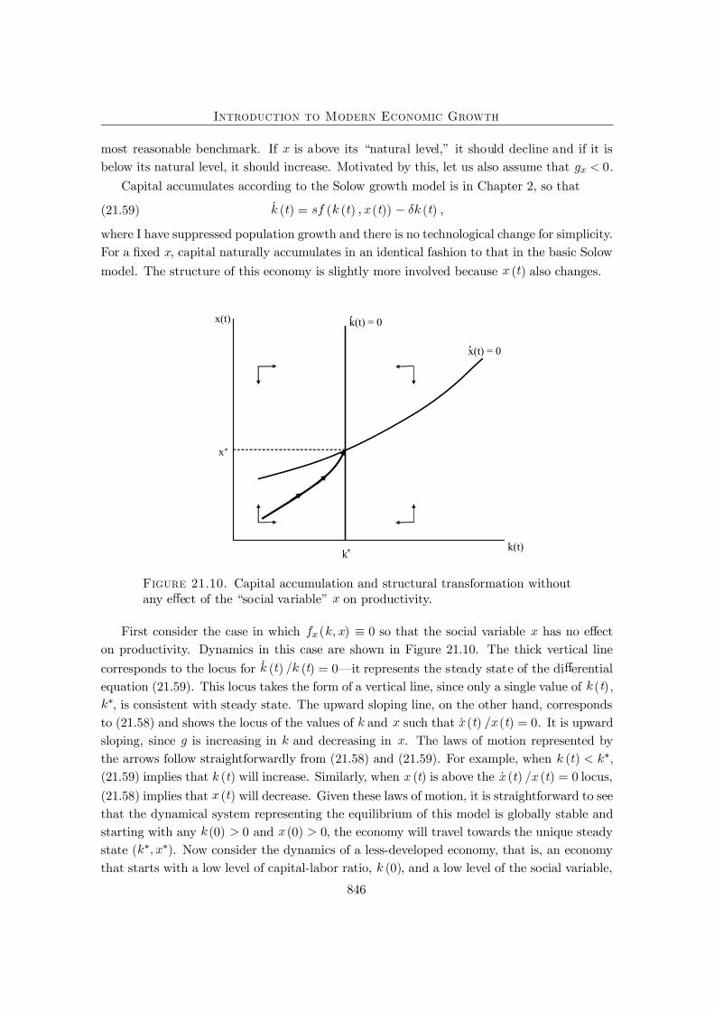
Introduction to Modern Economic Growth
most reasonable benchmark. If is above its �natural level,� it should decline and if it isbelow its natural level, it should increase. Motivated by this, let us also assume that 0.
Capital accumulates according to the Solow growth model is in Chapter 2, so that
(21.59) ú ( ) = ( ( ) ( )) ( )
where I have suppressed population growth and there is no technological change for simplicity.For a Þxed , capital naturally accumulates in an identical fashion to that in the basic Solowmodel. The structure of this economy is slightly more involved because ( ) also changes.
x(t)
k(t)
k(t) = 0
k*
x*
.x(t) = 0
.
Figure 21.10. Capital accumulation and structural transformation withoutany e ect of the �social variable� on productivity.
First consider the case in which ( ) 0 so that the social variable has no e ecton productivity. Dynamics in this case are shown in Figure 21.10. The thick vertical linecorresponds to the locus for ú ( ) ( ) = 0�it represents the steady state of the di erentialequation (21.59). This locus takes the form of a vertical line, since only a single value of ( ),, is consistent with steady state. The upward sloping line, on the other hand, corresponds
to (21.58) and shows the locus of the values of and such that ú ( ) ( ) = 0. It is upwardsloping, since is increasing in and decreasing in . The laws of motion represented bythe arrows follow straightforwardly from (21.58) and (21.59). For example, when ( ) ,(21.59) implies that ( ) will increase. Similarly, when ( ) is above the ú ( ) ( ) = 0 locus,(21.58) implies that ( ) will decrease. Given these laws of motion, it is straightforward to seethat the dynamical system representing the equilibrium of this model is globally stable andstarting with any (0) 0 and (0) 0, the economy will travel towards the unique steadystate ( ). Now consider the dynamics of a less-developed economy, that is, an economythat starts with a low level of capital-labor ratio, (0), and a low level of the social variable,
846
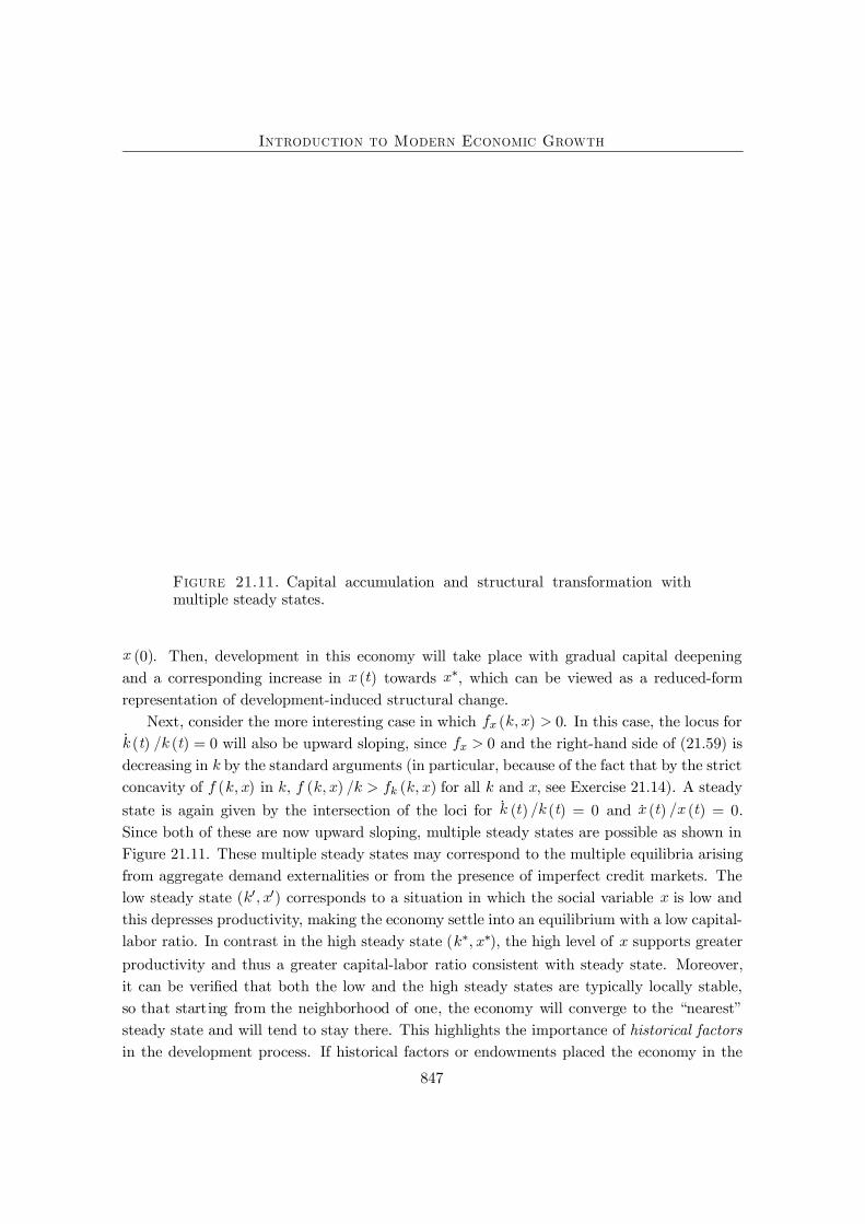
Introduction to Modern Economic Growth
Figure 21.11. Capital accumulation and structural transformation withmultiple steady states.
(0). Then, development in this economy will take place with gradual capital deepeningand a corresponding increase in ( ) towards , which can be viewed as a reduced-formrepresentation of development-induced structural change.
Next, consider the more interesting case in which ( ) 0. In this case, the locus forú ( ) ( ) = 0 will also be upward sloping, since 0 and the right-hand side of (21.59) isdecreasing in by the standard arguments (in particular, because of the fact that by the strictconcavity of ( ) in , ( ) ( ) for all and , see Exercise 21.14). A steadystate is again given by the intersection of the loci for ú ( ) ( ) = 0 and ú ( ) ( ) = 0.Since both of these are now upward sloping, multiple steady states are possible as shown inFigure 21.11. These multiple steady states may correspond to the multiple equilibria arisingfrom aggregate demand externalities or from the presence of imperfect credit markets. Thelow steady state ( 0 0) corresponds to a situation in which the social variable is low andthis depresses productivity, making the economy settle into an equilibrium with a low capital-labor ratio. In contrast in the high steady state ( ), the high level of supports greaterproductivity and thus a greater capital-labor ratio consistent with steady state. Moreover,it can be veriÞed that both the low and the high steady states are typically locally stable,so that starting from the neighborhood of one, the economy will converge to the �nearest�steady state and will tend to stay there. This highlights the importance of historical factorsin the development process. If historical factors or endowments placed the economy in the
847
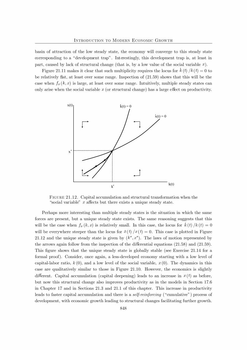
Introduction to Modern Economic Growth
basin of attraction of the low steady state, the economy will converge to this steady statecorresponding to a �development trap�. Interestingly, this development trap is, at least inpart, caused by lack of structural change (that is, by a low value of the social variable ).
Figure 21.11 makes it clear that such multiplicity requires the locus for ú ( ) ( ) = 0 tobe relatively ßat, at least over some range. Inspection of (21.59) shows that this will be thecase when ( ) is large, at least over some range. Intuitively, multiple steady states canonly arise when the social variable (or structural change) has a large e ect on productivity.
x(t)
k(t)
k(t) = 0
k*
x*
.x(t) = 0
.
Figure 21.12. Capital accumulation and structural transformation when the�social variable� a ects but there exists a unique steady state.
Perhaps more interesting than multiple steady states is the situation in which the sameforces are present, but a unique steady state exists. The same reasoning suggests that thiswill be the case when ( ) is relatively small. In this case, the locus for ú ( ) ( ) = 0will be everywhere steeper than the locus for ú ( ) ( ) = 0. This case is plotted in Figure21.12 and the unique steady state is given by ( ). The laws of motion represented bythe arrows again follow from the inspection of the di erential equations (21.58) and (21.59).This Þgure shows that the unique steady state is globally stable (see Exercise 21.14 for aformal proof). Consider, once again, a less-developed economy starting with a low level ofcapital-labor ratio, (0), and a low level of the social variable, (0). The dynamics in thiscase are qualitatively similar to those in Figure 21.10. However, the economics is slightlydi erent. Capital accumulation (capital deepening) leads to an increase in ( ) as before,but now this structural change also improves productivity as in the models in Section 17.6in Chapter 17 and in Sections 21.3 and 21.1 of this chapter. This increase in productivityleads to faster capital accumulation and there is a self-reinforcing (�cumulative�) process ofdevelopment, with economic growth leading to structural changes facilitating further growth.
848
Introduction to Modern Economic Growth
However, since the e ect of on productivity is limited, this process ultimately takes ustowards a unique steady state.
This reduced-form representation of structural change, therefore, captures some of thesalient features emphasized in this chapter. It is not meant to be a uniÞed model; on thecontrary, rather than combining multiple dimensions of structural change, it presents an ab-stract representation emphasizing how the process of development, corresponding to capitalaccumulation, can go hand-in-hand with structural change, which may in turn increase pro-ductivity and facilitate further capital accumulation. Developing a truly uniÞed model ofeconomic development and structural change is an area for future work.
21.8. Taking Stock
This chapter provided a large number of models focusing on various aspects of the struc-tural transformation accompanying economic development. As emphasized in the previoussection, there is no single framework unifying all these distinct aspects, even though thereare many common themes in these models. The previous section was an attempt to bringout these common themes. Instead of repeating these commonalities, I would like to con-clude by pointing out that many of the topics covered in this chapter are at the frontier ofcurrent research and much still remains to be done. Economic development is intimatelylinked to economic growth, but it may require di erent, even specialized, models that do notjust focus on balanced growth and the orderly growth behavior captured by the neoclassicaland endogenous technology models. These models may also need to take market failures andhow these market failures might change over time more seriously. This view stems from therecognition that the essence of economic development is the process of structural transforma-tion, including Þnancial development, the demographic transition, migration, urbanization,organizational change and other social changes.
Another potentially important aspect of economic development is the possibility thatthe ine ciencies in the organization of production, credit markets and product markets mayculminate in potential development traps. These ine ciencies may stem from lack of coor-dination in the presence of aggregate demand externalities or from the interaction betweenimperfect credit markets and human capital investments. These topics not only highlightsome of the questions that need to be addressed for understanding the process of economicdevelopment, but they also bring a range of issues that are often secondary in the standardgrowth literature to the forefront of analysis. These include, among other things, the orga-nization of Þnancial markets, the distribution of income and wealth and issues of incentives,such as problems of moral hazard, adverse selection and incomplete contracts both in creditmarkets and in production relationships.
The recognition that the analysis of economic development necessitates a special focuson these topics also opens the way for a more constructive interaction between empiricaldevelopment studies and the theories of economic development surveyed in this chapter. Asalready noted above, there is now a large literature on empirical development economics,
849
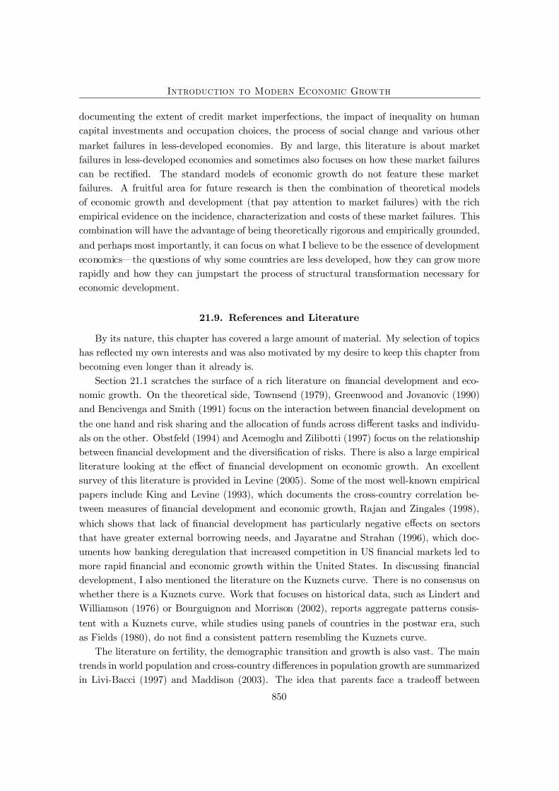
Introduction to Modern Economic Growth
documenting the extent of credit market imperfections, the impact of inequality on humancapital investments and occupation choices, the process of social change and various othermarket failures in less-developed economies. By and large, this literature is about marketfailures in less-developed economies and sometimes also focuses on how these market failurescan be rectiÞed. The standard models of economic growth do not feature these marketfailures. A fruitful area for future research is then the combination of theoretical modelsof economic growth and development (that pay attention to market failures) with the richempirical evidence on the incidence, characterization and costs of these market failures. Thiscombination will have the advantage of being theoretically rigorous and empirically grounded,and perhaps most importantly, it can focus on what I believe to be the essence of developmenteconomics�the questions of why some countries are less developed, how they can grow morerapidly and how they can jumpstart the process of structural transformation necessary foreconomic development.
21.9. References and Literature
By its nature, this chapter has covered a large amount of material. My selection of topicshas reßected my own interests and was also motivated by my desire to keep this chapter frombecoming even longer than it already is.
Section 21.1 scratches the surface of a rich literature on Þnancial development and eco-nomic growth. On the theoretical side, Townsend (1979), Greenwood and Jovanovic (1990)and Bencivenga and Smith (1991) focus on the interaction between Þnancial development onthe one hand and risk sharing and the allocation of funds across di erent tasks and individu-als on the other. Obstfeld (1994) and Acemoglu and Zilibotti (1997) focus on the relationshipbetween Þnancial development and the diversiÞcation of risks. There is also a large empiricalliterature looking at the e ect of Þnancial development on economic growth. An excellentsurvey of this literature is provided in Levine (2005). Some of the most well-known empiricalpapers include King and Levine (1993), which documents the cross-country correlation be-tween measures of Þnancial development and economic growth, Rajan and Zingales (1998),which shows that lack of Þnancial development has particularly negative e ects on sectorsthat have greater external borrowing needs, and Jayaratne and Strahan (1996), which doc-uments how banking deregulation that increased competition in US Þnancial markets led tomore rapid Þnancial and economic growth within the United States. In discussing Þnancialdevelopment, I also mentioned the literature on the Kuznets curve. There is no consensus onwhether there is a Kuznets curve. Work that focuses on historical data, such as Lindert andWilliamson (1976) or Bourguignon and Morrison (2002), reports aggregate patterns consis-tent with a Kuznets curve, while studies using panels of countries in the postwar era, suchas Fields (1980), do not Þnd a consistent pattern resembling the Kuznets curve.
The literature on fertility, the demographic transition and growth is also vast. The maintrends in world population and cross-country di erences in population growth are summarizedin Livi-Bacci (1997) and Maddison (2003). The idea that parents face a tradeo between
850
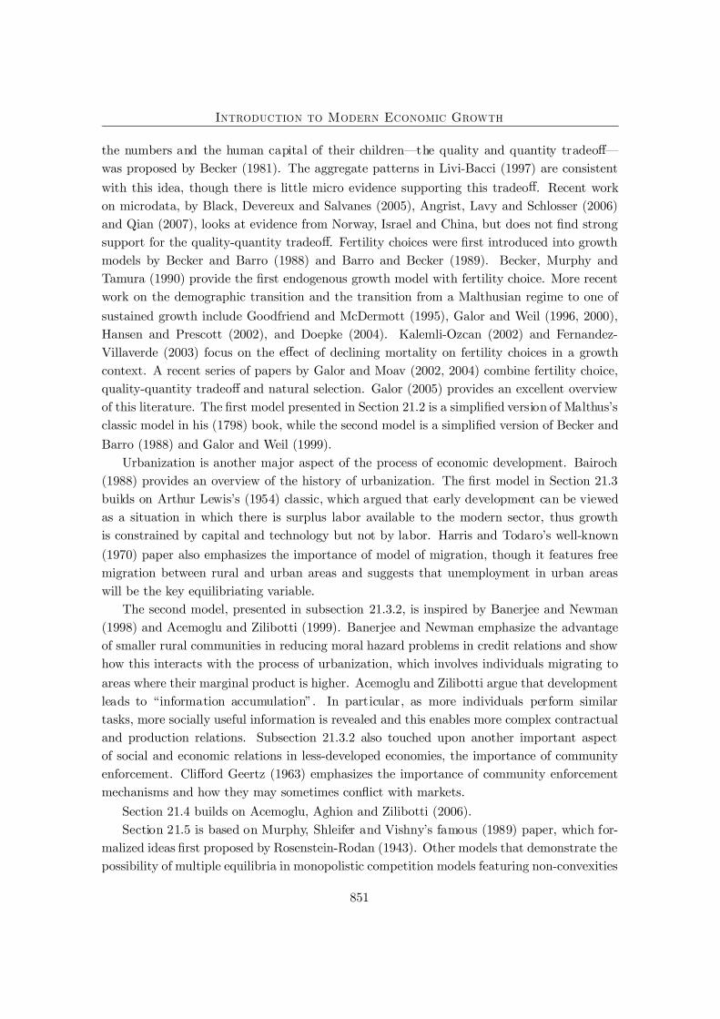
Introduction to Modern Economic Growth
the numbers and the human capital of their children�the quality and quantity tradeo �was proposed by Becker (1981). The aggregate patterns in Livi-Bacci (1997) are consistentwith this idea, though there is little micro evidence supporting this tradeo . Recent workon microdata, by Black, Devereux and Salvanes (2005), Angrist, Lavy and Schlosser (2006)and Qian (2007), looks at evidence from Norway, Israel and China, but does not Þnd strongsupport for the quality-quantity tradeo . Fertility choices were Þrst introduced into growthmodels by Becker and Barro (1988) and Barro and Becker (1989). Becker, Murphy andTamura (1990) provide the Þrst endogenous growth model with fertility choice. More recentwork on the demographic transition and the transition from a Malthusian regime to one ofsustained growth include Goodfriend and McDermott (1995), Galor and Weil (1996, 2000),Hansen and Prescott (2002), and Doepke (2004). Kalemli-Ozcan (2002) and Fernandez-Villaverde (2003) focus on the e ect of declining mortality on fertility choices in a growthcontext. A recent series of papers by Galor and Moav (2002, 2004) combine fertility choice,quality-quantity tradeo and natural selection. Galor (2005) provides an excellent overviewof this literature. The Þrst model presented in Section 21.2 is a simpliÞed version of Malthus�sclassic model in his (1798) book, while the second model is a simpliÞed version of Becker andBarro (1988) and Galor and Weil (1999).
Urbanization is another major aspect of the process of economic development. Bairoch(1988) provides an overview of the history of urbanization. The Þrst model in Section 21.3builds on Arthur Lewis�s (1954) classic, which argued that early development can be viewedas a situation in which there is surplus labor available to the modern sector, thus growthis constrained by capital and technology but not by labor. Harris and Todaro�s well-known(1970) paper also emphasizes the importance of model of migration, though it features freemigration between rural and urban areas and suggests that unemployment in urban areaswill be the key equilibriating variable.
The second model, presented in subsection 21.3.2, is inspired by Banerjee and Newman(1998) and Acemoglu and Zilibotti (1999). Banerjee and Newman emphasize the advantageof smaller rural communities in reducing moral hazard problems in credit relations and showhow this interacts with the process of urbanization, which involves individuals migrating toareas where their marginal product is higher. Acemoglu and Zilibotti argue that developmentleads to �information accumulation�. In particular, as more individuals perform similartasks, more socially useful information is revealed and this enables more complex contractualand production relations. Subsection 21.3.2 also touched upon another important aspectof social and economic relations in less-developed economies, the importance of communityenforcement. Cli ord Geertz (1963) emphasizes the importance of community enforcementmechanisms and how they may sometimes conßict with markets.
Section 21.4 builds on Acemoglu, Aghion and Zilibotti (2006).Section 21.5 is based on Murphy, Shleifer and Vishny�s famous (1989) paper, which for-
malized ideas Þrst proposed by Rosenstein-Rodan (1943). Other models that demonstrate thepossibility of multiple equilibria in monopolistic competition models featuring non-convexities
851
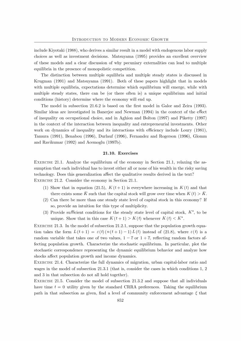
Introduction to Modern Economic Growth
include Kiyotaki (1988), who derives a similar result in a model with endogenous labor supplychoices as well as investment decisions. Matsuyama (1995) provides an excellent overviewof these models and a clear discussion of why pecuniary externalities can lead to multipleequilibria in the presence of monopolistic competition.
The distinction between multiple equilibria and multiple steady states is discussed inKrugman (1991) and Matsuyama (1991). Both of these papers highlight that in modelswith multiple equilibria, expectations determine which equilibrium will emerge, while withmultiple steady states, there can be (or there often is) a unique equilibrium and initialconditions (history) determine where the economy will end up.
The model in subsection 21.6.2 is based on the Þrst model in Galor and Zeira (1993).Similar ideas are investigated in Banerjee and Newman (1994) in the context of the e ectof inequality on occupational choice, and in Aghion and Bolton (1997) and Piketty (1997)in the context of the interaction between inequality and entrepreneurial investments. Otherwork on dynamics of inequality and its interactions with e ciency include Loury (1981),Tamura (1991), Benabou (1996), Durlauf (1996), Fernandez and Rogerson (1996), Glommand Ravikumar (1992) and Acemoglu (1997b).
21.10. Exercises
Exercise 21.1. Analyze the equilibrium of the economy in Section 21.1, relaxing the as-sumption that each individual has to invest either all or none of his wealth in the risky savingtechnology. Does this generalization a ect the qualitative results derived in the text?Exercise 21.2. Consider the economy in Section 21.1.
(1) Show that in equation (21.5), ( + 1) is everywhere increasing in ( ) and thatthere exists some ¯ such that the capital stock will grow over time when ( ) ¯ .
(2) Can there be more than one steady state level of capital stock in this economy? Ifso, provide an intuition for this type of multiplicity.
(3) Provide su cient conditions for the steady state level of capital stock, , to beunique. Show that in this case ( + 1) ( ) whenever ( ) .
Exercise 21.3. In the model of subsection 21.2.1, suppose that the population growth equa-tion takes the form ( + 1) = ( ) ( ( + 1) 1) ( ) instead of (21.8), where ( ) is arandom variable that takes one of two values, 1 or 1 + , reßecting random factors af-fecting population growth. Characterize the stochastic equilibrium. In particular, plot thestochastic correspondence representing the dynamic equilibrium behavior and analyze howshocks a ect population growth and income dynamics.Exercise 21.4. Characterize the full dynamics of migration, urban capital-labor ratio andwages in the model of subsection 21.3.1 (that is, consider the cases in which conditions 1, 2and 3 in that subsection do not all hold together).Exercise 21.5. Consider the model of subsection 21.3.2 and suppose that all individualshave time = 0 utility given by the standard CRRA preferences. Taking the equilibriumpath in that subsection as given, Þnd a level of community enforcement advantage that
852
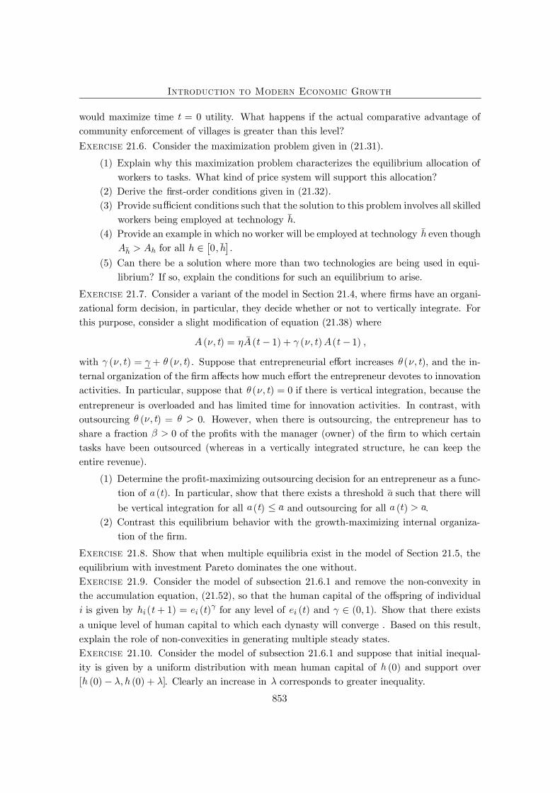
Introduction to Modern Economic Growth
would maximize time = 0 utility. What happens if the actual comparative advantage ofcommunity enforcement of villages is greater than this level?Exercise 21.6. Consider the maximization problem given in (21.31).
(1) Explain why this maximization problem characterizes the equilibrium allocation ofworkers to tasks. What kind of price system will support this allocation?
(2) Derive the Þrst-order conditions given in (21.32).(3) Provide su cient conditions such that the solution to this problem involves all skilled
workers being employed at technology ¯.(4) Provide an example in which no worker will be employed at technology ¯ even though
¯ for all£0 ¯¤.
(5) Can there be a solution where more than two technologies are being used in equi-librium? If so, explain the conditions for such an equilibrium to arise.
Exercise 21.7. Consider a variant of the model in Section 21.4, where Þrms have an organi-zational form decision, in particular, they decide whether or not to vertically integrate. Forthis purpose, consider a slight modiÞcation of equation (21.38) where
( ) = ¯ ( 1) + ( ) ( 1)
with ( ) = + ( ). Suppose that entrepreneurial e ort increases ( ), and the in-ternal organization of the Þrm a ects how much e ort the entrepreneur devotes to innovationactivities. In particular, suppose that ( ) = 0 if there is vertical integration, because theentrepreneur is overloaded and has limited time for innovation activities. In contrast, withoutsourcing ( ) = 0. However, when there is outsourcing, the entrepreneur has toshare a fraction 0 of the proÞts with the manager (owner) of the Þrm to which certaintasks have been outsourced (whereas in a vertically integrated structure, he can keep theentire revenue).
(1) Determine the proÞt-maximizing outsourcing decision for an entrepreneur as a func-tion of ( ). In particular, show that there exists a threshold ¯ such that there willbe vertical integration for all ( ) ¯ and outsourcing for all ( ) ¯.
(2) Contrast this equilibrium behavior with the growth-maximizing internal organiza-tion of the Þrm.
Exercise 21.8. Show that when multiple equilibria exist in the model of Section 21.5, theequilibrium with investment Pareto dominates the one without.Exercise 21.9. Consider the model of subsection 21.6.1 and remove the non-convexity inthe accumulation equation, (21.52), so that the human capital of the o spring of individualis given by ( + 1) = ( ) for any level of ( ) and (0 1). Show that there existsa unique level of human capital to which each dynasty will converge . Based on this result,explain the role of non-convexities in generating multiple steady states.Exercise 21.10. Consider the model of subsection 21.6.1 and suppose that initial inequal-ity is given by a uniform distribution with mean human capital of (0) and support over[ (0) (0) + ]. Clearly an increase in corresponds to greater inequality.
853
Introduction to Modern Economic Growth
(1) Show that when (0) is su ciently small, an increase in will increase long-run av-erage human capital and income, whereas when (0) is su ciently large, an increasein will reduce them. [Hint: use Figures 21.8-21.9].
(2) What other types of distributions (besides uniform) would lead to the same result?(3) Show that the same result generalizes to the model of 21.6.2.(4) On the basis of this result, discuss whether we should expect greater inequality to
lead to higher income in poor societies and lower income in rich societies. (If youranswer is no, then sketch an environment in which this will not be the case).
Exercise 21.11. Consider the model presented in subsection 21.6.2. Make the following twomodiÞcations. First, the utility function is now
(21.60) (1 ) (1 ) 1
and second, unskilled agents receive a wage of + where is a mean-zero random shock.
(1) Suppose that is distributed with support [ ], and show that if is su cientlyclose to 0, then the multiple steady states characterized in 21.6.2 �survive� in thesense that depending on their initial conditions some dynasties become high skilledand others become low skilled.
(2) Why was it convenient to change the utility function from the log form used in thetext to (21.60)?
(3) Now suppose that is distributed with support [ ), where . Show thatin this case there is a unique ergodic distribution of wealth and no poverty trap.Explain why the results here are di erent from those in part 1?
(4) How would the results be di erent if, in addition, the skilled wage is equal to + ,where is another mean-zero random shock? [Hint: simply sketch the analysis andthe structure of the equilibrium without repeating the full analysis of part 3].
Exercise 21.12. (1) In the model of subsection 21.6.2, suppose that each individualcan run away without paying his debts, and if he does so, he will never be caught.However, a bank can prevent this by paying a monitoring cost per unit of borrow-ing equal to . Suppose that there are many banks competing a la Bertrand forlending opportunities. Under these assumptions, show that all bank lending will beaccompanied with monitoring, and the lending rate will satisfy = + . Showthat in this case all of the results in the text apply.
(2) Next suppose that the bank can prevent individual from running away by paying aÞxed monitoring cost of . Under the same assumptions as in part 1 above showthat in this case the interest rate charged to an individual that borrows an amount
will be ( ) = + ( ). Given this assumption, characterize theequilibrium of the model in subsection 21.6.2. How do the conclusions change inthis case?
(3) Next suppose that there is no way of preventing running away by individuals, butif an individual runs away, he will be caught with probability , and in this case,
854
Introduction to Modern Economic Growth
a fraction (0 1) of his income will be conÞscated. Given this assumption,characterize equilibrium dynamics of the model in subsection 21.6.2. How do theconclusions change in this case?
(4) Now consider an increase in (for a given level of ) so that the skill premium inthe economy increases. In which of the three scenarios outlined above will this havethe largest e ect on human capital investments?
Exercise 21.13. In this exercise, you are asked to study Banerjee and Newman�s (1994)model of occupational choice. The utility of each individual is again (1 ) (1 ) 1
, where denotes whether the individual is exerting e ort, with cost of e ort normalizedto 1. Each agent chooses one of four possible occupations. These are (1) subsistence and nowork, which leads to no labor income and has a rate of return on assets equal to � 1 ;(2) work for a wage ; (3) self-employment, which requires investment plus the labor of theindividual; and (4) entrepreneurship, which requires investment plus the employment ofworkers, and the individual himself becomes the boss, monitoring the workers (and does
not take part in production). All occupations other than subsistence involve e ort. Let usassume that both entrepreneurship and self-employment generate a rate of return greaterthan subsistence (that is, the mean return for both activities is ¯ �).
(1) Derive the indirect utility function associated with the preferences above. Show thatno individual will work as a worker for a wage less than 1.
(2) Assume that [ (¯ �) 1] 1 (¯ �) 1 0. Interpret this assumption.[Hint: it relates the proÞtabilities of entrepreneurship and self-employment at theminimum possible wage of 1].
(3) Suppose that only agents that have wealth can borrow enough to becomeself-employed and only agents that have wealth can borrow tobecome an entrepreneur. Provide intuition for these borrowing constraints.
(4) Now compute the expected indirect utility from the four occupations. Show that if¯ ( 1) (¯ �) , then self-employment is preferred to entrepreneurship.
(5) Suppose the wealth distribution at time is given by ( ). On the basis of theresults in part 4, show that the demand for labor in this economy is given by
= 0 if ¯[0 (1 ( ))] if = ¯= (1 ( )) if ¯
(6) Let � (¯ �) ¯. Then, show that the supply of labor is given by
= 0 if 1[0 ( )] if = 1= ( ) if 1 �[ ( ) 1] if = �= 1 if �
855
Introduction to Modern Economic Growth
(7) Show that if ( ) [1 ( )], there will be an excess supply of labor andthe equilibrium wage rate will be = 1. Show that if ( ) [1 ( )],there will be an excess demand for labor and the equilibrium wage rate will be = ¯.
(8) Now derive the individual wealth (bequest) dynamics (for a worker with wealth) as follows: (1) subsistence and no work: ( ) = � ; (2) worker: ( ) =(� + ); (3) self-employment: ( ) = (¯ + � ( )); (4) entrepreneurship:( ) = (¯ + � ( ) ). Explain the intuition for each of these expres-sions.
(9) Now using these wealth dynamics show that multiple steady states with di erentwealth distributions and occupational choices are possible. In particular, showthat the steady-state wealth level of a worker when the wage rate is will be( ) = (1 �), while the steady-state wealth level of a self-employed individ-
ual will be = (¯ �) (1 �), and the wealth level of an entrepreneur willbe ( ) = (¯ � ) (1 �). Now show that when ( = 1)and ( = ¯) , a steady state in which the equilibrium wage rate is equalto = 1 would involve workers not accumulating su cient wealth to become self-employed, while entrepreneurs accumulate enough wealth to remain entrepreneurs.Explain why this is the case. [Hint: it depends on the equilibrium wage rate].
(10) Given the result in part 9, show that if we start with a wealth distribution suchthat (1 ( )) ( ), the steady state will involve an equilibrium wage= 1 and no self-employment, whereas if we start with (1 ( )) ( ),
the equilibrium wage would be = ¯ and there will be self-employment. Contrastthe level of output in these two steady states.
(11) Is the comparison of the steady states in terms of output in this model plausible?Is it consistent with historical evidence? What are the pros and cons of this modelrelative to the Galor-Zeira model in subsection 21.6.2?
Exercise 21.14. This exercise asks you to analyze the dynamics of the reduced-form modelin Section 21.7 more formally.
(1) Show that when 0, the locus for ú = 0 implied by (21.58) is an upwardsloping curve.
(2) Consider the di erential equations (21.58) and (21.59), and a steady state ( ).By linearizing the two di erential equations around ( ), show that if ( )is su ciently small, the steady state is locally stable.
(3) Provide a uniform bound on ( ) so that there exists a unique steady state.Show that when this bound applies, the unique steady state is globally stable.
(4) Construct a parameterized example where there are multiple steady states. Interpretthe conditions necessary for this example. Do you Þnd them economically likely?
856