AGT 関係式とその一般化に向け

て(String Advanced Lectures No.22)

高エネルギー加速器研究機構 (KEK)

素粒子原子核研究所 (IPNS)

柴　正太郎

2010 年 7 月 5 日（月） 14:00-15:40

Contents

1. Gaiotto’s discussion

2. AGT relation for SU(2) quiver theories

3. AGT-W relation for SU(N) quiver

theories

4. AdS/CFT correspondence of AGT’s

system

Gaiotto’s discussion

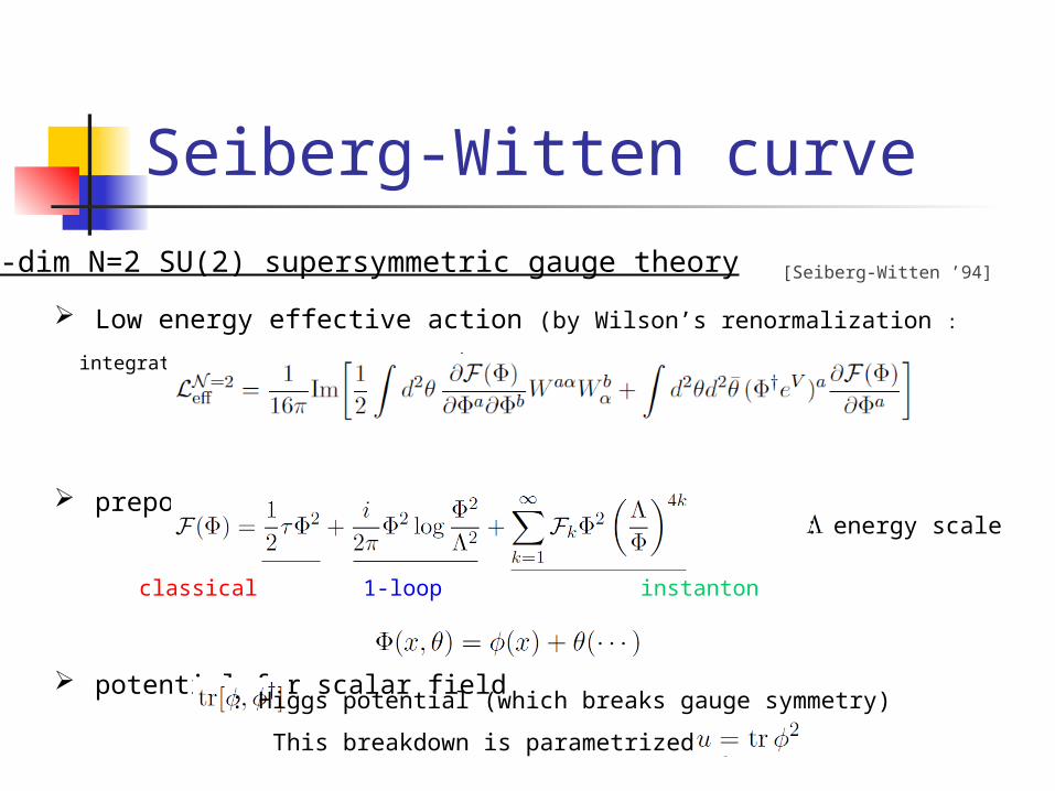
Seiberg-Witten curve

Low energy effective action (by Wilson’s renormalization : integration out of

massive fields)

prepotential

potential for scalar field

4-dim N=2 SU(2) supersymmetric gauge theory [Seiberg-Witten ’94]

classical 1-loop instanton

: energy scale

: Higgs potential (which breaks gauge symmetry)

This breakdown is parametrized by

u (VEV) : shift of color brane

mass : shift of flavor

brane

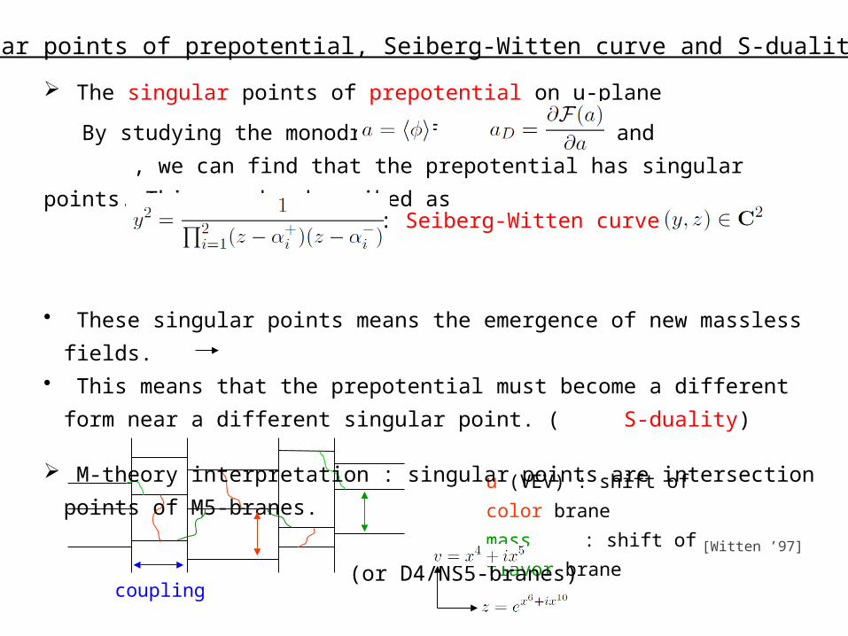
Singular points of prepotential, Seiberg-Witten curve and S-duality

The singular points of prepotential on u-plane

By studying the monodromy of and , we can find

that the prepotential has singular points. This can be described as

• These singular points means the emergence of new massless fields.• This means that the prepotential must become a different form near

a different singular point. ( S-duality)

M-theory interpretation : singular points are intersection points of M5-

branes.

(or D4/NS5-

branes)

[Witten ’97]

: Seiberg-Witten curve in

coupling

SU(2) generalized quivers[Gaiotto ’09]

SU(2) gauge theory with 4 fundamental flavors (hypermultiplets)

S-duality group SL(2,Z)

coupling const. :

flavor sym. : SO(8) ⊃ SO(4)×SO(4) ～

[SU(2)a×SU(2)b]×[SU(2)c×SU(2)d]

: (elementary) quark

: monopole

: dyon

D4

NS5

Subgroup of S-duality without permutation of masses

In massive case, we especially consider this subgroup.

• mass : mass parameters can be associated to each SU(2) flavor.

Then the mass eigenvalues of four hypermultiplets in 8v is ,

.

• coupling : cross ratio (moduli) of the four punctures, i.e. z =

Actually, this is equal to the exponential of the UV coupling

→ This is an aspect of correspondence between the 4-dim N=2 SU(2)

gauge theory and the 2-dim Riemann surface with punctures.

SU(2) gauge theory with massive fundamental hypermultiplets

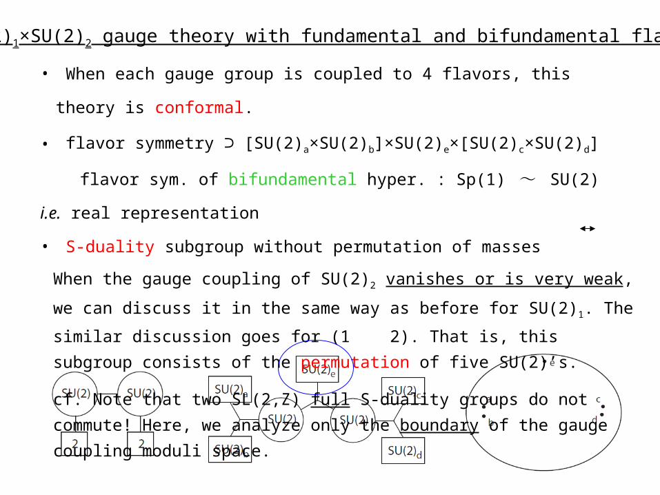
SU(2)1×SU(2)2 gauge theory with fundamental and bifundamental flavors

• When each gauge group is coupled to 4 flavors, this theory is

conformal.

• flavor symmetry ⊃ [SU(2)a×SU(2)b]×SU(2)e×[SU(2)c×SU(2)d]

flavor sym. of bifundamental hyper. : Sp(1) ～ SU(2) i.e. real

representation

• S-duality subgroup without permutation of masses

When the gauge coupling of SU(2)2 vanishes or is very weak, we can

discuss it in the same way as before for SU(2)1. The similar discussion

goes for (1 2). That is, this subgroup consists of the permutation of

five SU(2)’s.

cf. Note that two SL(2,Z) full S-duality groups do not commute! Here,

we analyze only the boundary of the gauge coupling moduli space.

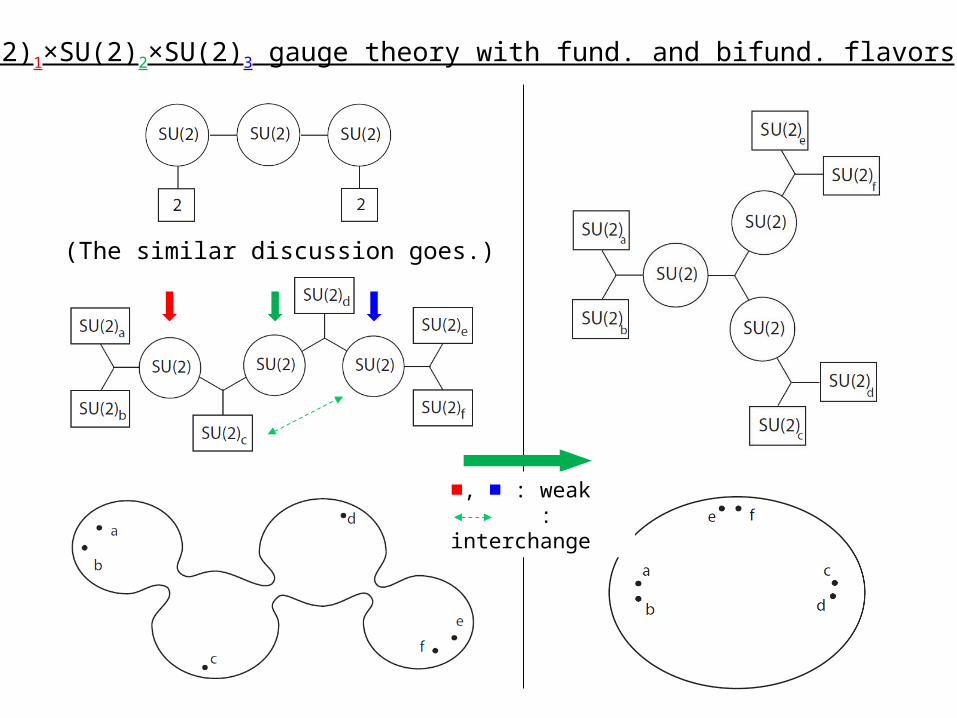
SU(2)1×SU(2)2×SU(2)3 gauge theory with fund. and bifund. flavors

(The similar discussion goes.)

■, ■ : weak : interchange

turn on/off a gauge coupling

For more generalized SU(2) quivers : more gauge groups, loops…

Seiberg-Witten curve for quiver SU(2) gauge theories

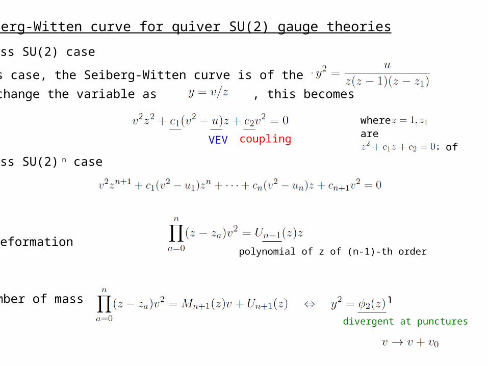
massless SU(2) case

In this case, the Seiberg-Witten curve is of the form

If we change the variable as , this becomes

massless SU(2) n case

or

mass deformation

The number of mass parameters is n+3, because of the freedom .

where are the solutions of

VEV coupling

polynomial of z of (n-1)-th order

divergent at punctures

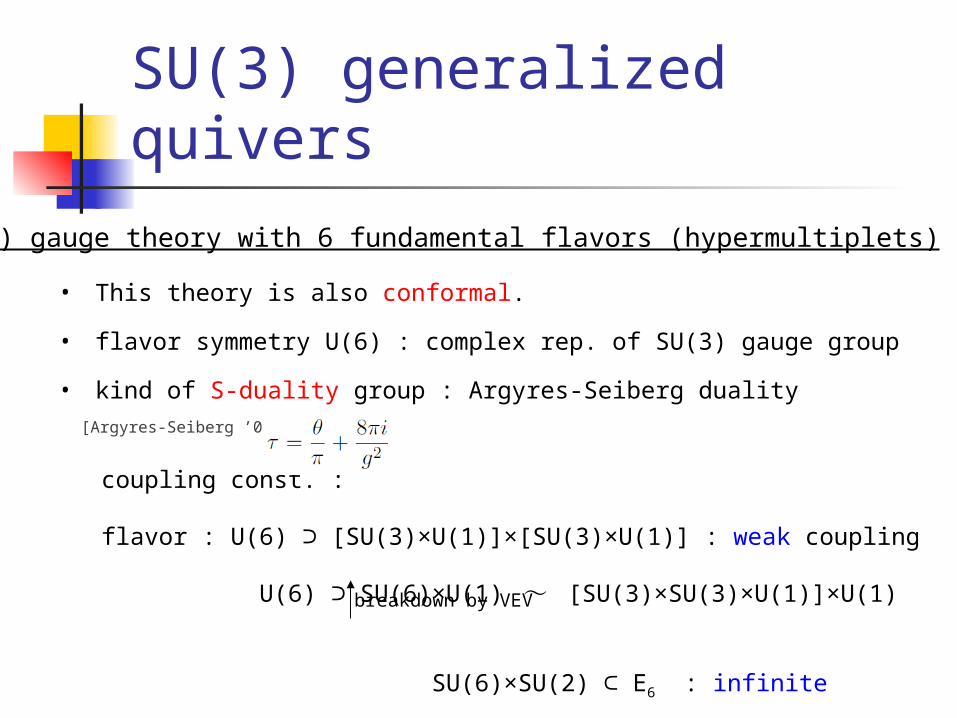
SU(3) generalized quivers

SU(3) gauge theory with 6 fundamental flavors (hypermultiplets)

• This theory is also conformal.

• flavor symmetry U(6) : complex rep. of SU(3) gauge group

• kind of S-duality group : Argyres-Seiberg duality [Argyres-Seiberg ’07]

coupling const. :

flavor : U(6) ⊃ [SU(3)×U(1)]×[SU(3)×U(1)] : weak coupling

U(6) ⊃ SU(6)×U(1) ～ [SU(3)×SU(3)×U(1)]×U(1)

SU(6)×SU(2) ⊂ E6 : infinite coupling of SU(3) theory

Moreover, weakly coupled gauge group becomes SU(2) instead of

SU(3) !

breakdown by VEV

Argyres-Seiberg duality for SU(3) gauge theory

infinite coupling

D4

NS5

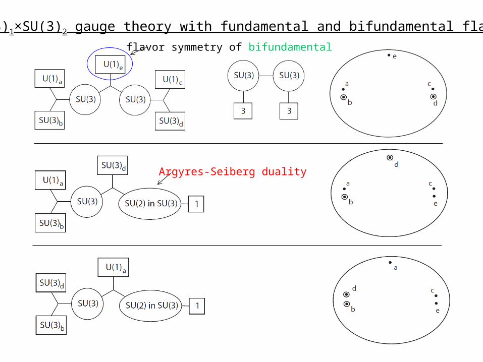
SU(3)1×SU(3)2 gauge theory with fundamental and bifundamental flavors

flavor symmetry of bifundamental

Argyres-Seiberg duality

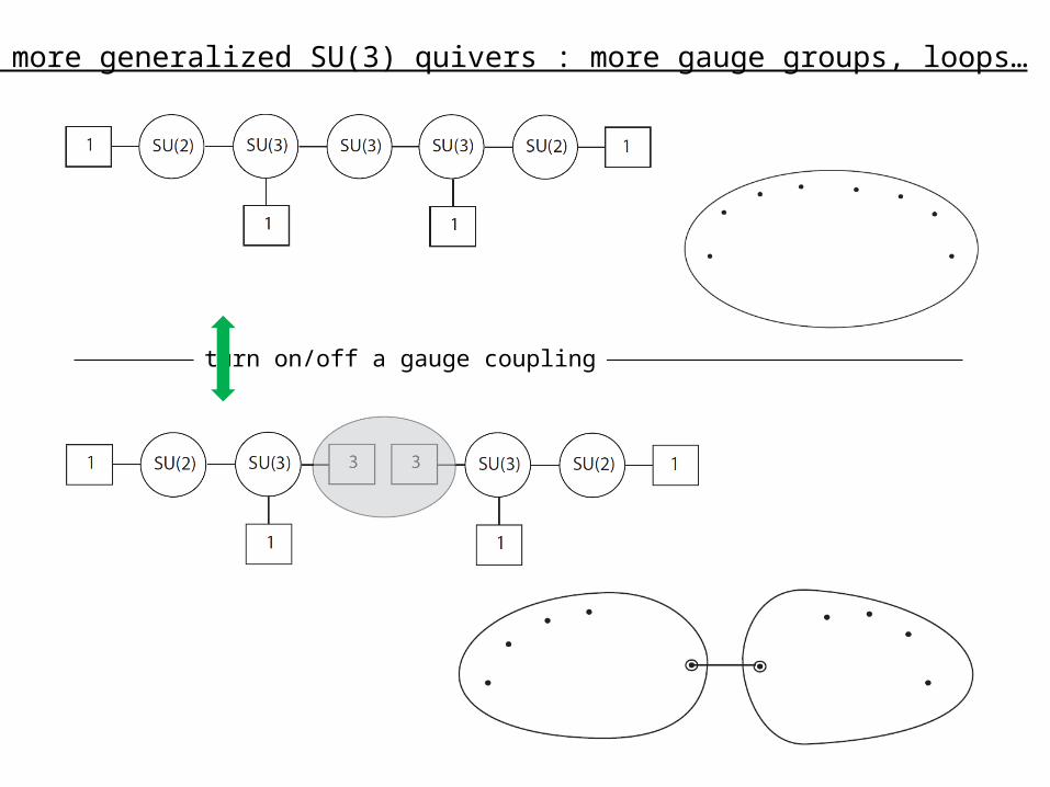
For more generalized SU(3) quivers : more gauge groups, loops…

turn on/off a gauge coupling

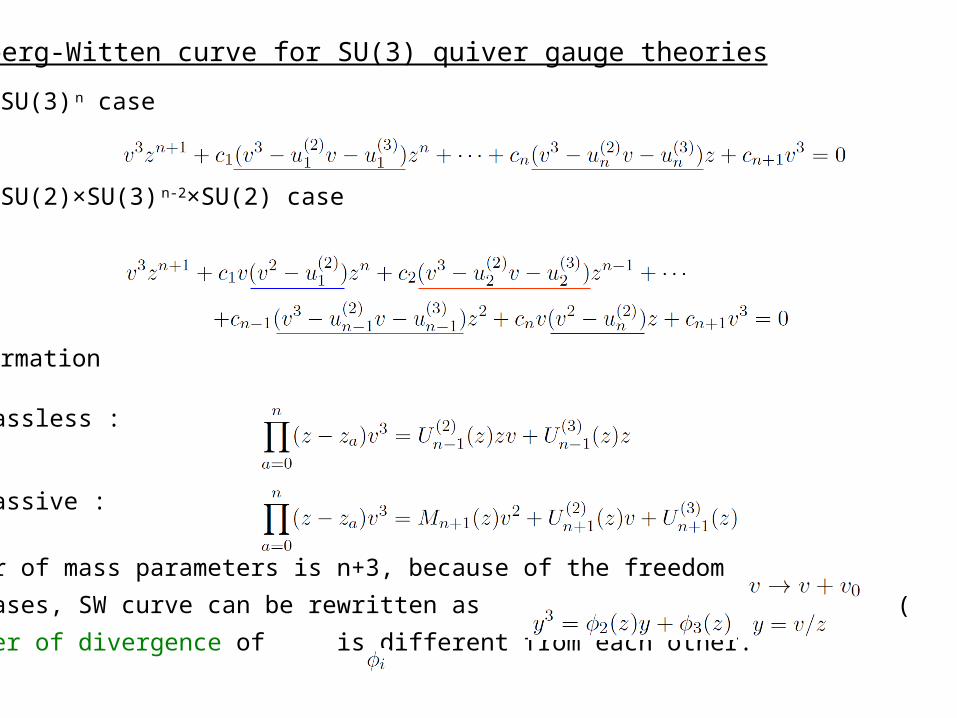
Seiberg-Witten curve for SU(3) quiver gauge theories

massless SU(3) n case

massless SU(2)×SU(3) n-2×SU(2) case

mass deformation

massless :

massive :

The number of mass parameters is n+3, because of the freedom .

In both cases, SW curve can be rewritten as ( ),

but the order of divergence of is different from each other.

SU(N) generalized quivers

Seiberg-Witten curve in this case is of the form

The variety of quiver gauge group

where

is reflected in the various order of divergence of 　　 at punctures.

For example…

Seiberg-Witten curve for massless SU(N) quiver gauge theories

SU(2) quiver case

• order of divergence :

• mass parameters :

• flavor symmetry : SU(2)

SU(3) quiver case

• order of divergence :

• mass parameters :

• flavor symmetry : U(1) SU(3)

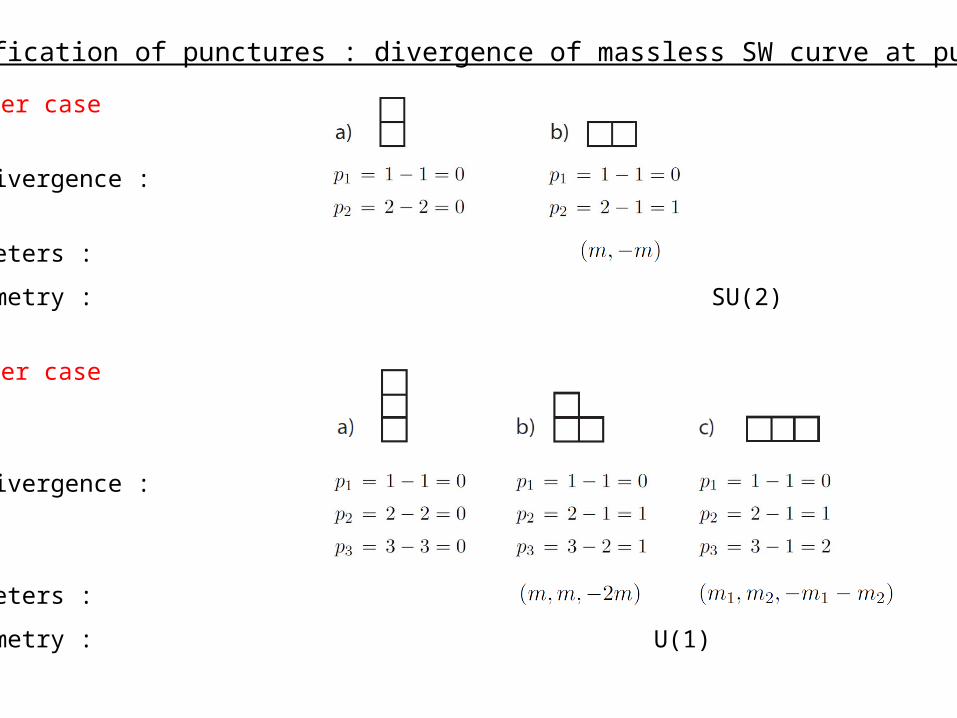
Classification of punctures : divergence of massless SW curve at punctures

SU(3) quiver case

corresponding puncture :

SU(4) quiver case (and the natural analogy is valid for general SU(N) case)

Classification of punctures : divergence of massless SW curve at punctures

AGT relation for SU(2)

quivers

SU(2) partition function

We now consider only the linear quiver gauge theories in AGT relation.

Gaiotto’s discussion

Nekrasov’s partition function of 4-dim gauge theory

Action

classical part

1-loop correction : more than 1-loop is cancelled, because of N=2

SUSY.

instanton correction : Nekrasov’s calculation with Young tableaux

Parameters

coupling constants

masses of fundamental / antifund. / bifund. fields and VEV’s of gauge

fields

deformation parameters :

background of graviphoton or deformation (rotation) of extra

dimensions

(Note that they are different from Gaiotto’s ones!)

Now we calculate Nekrasov’s partition function of 4-dim SU(2) quiver

gauge theory as the quantity of interest.

D4

NS5

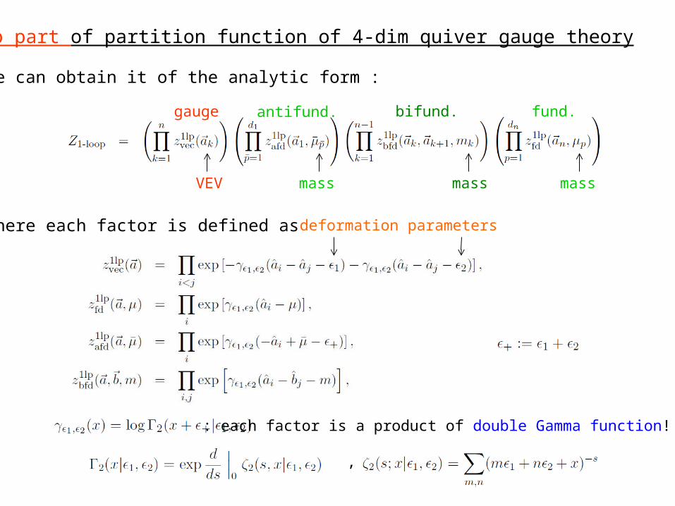
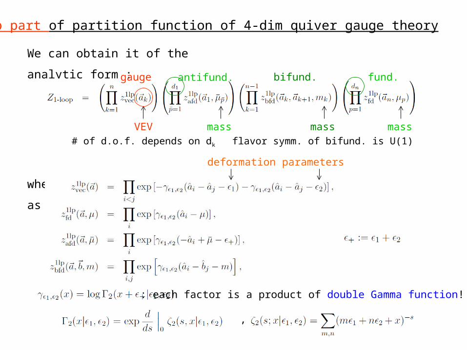
1-loop part of partition function of 4-dim quiver gauge theory

We can obtain it of the analytic form :

where each factor is defined as

: each factor is a product of double Gamma function!

,

gauge antifund. bifund. fund.

mass massmassVEV

deformation parameters

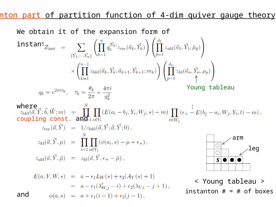
We obtain it of the expansion form of instanton

number :

where : coupling const. and

and

Instanton part of partition function of 4-dim quiver gauge theory

Young tableau

< Young tableau >

instanton # = # of boxes

leg

arm

The Nekrasov partition function for the simple case of SU(2) with four

flavors is

Since the mass dimension of is 1, so we fix the scale as ,

. (by definition)

Mass parameters : mass eigenvalues of four hypermultiplets

• : mass parameters of

• : mass parameters of

VEV’s : we set --- decoupling of U(1) (i.e. trace)

part.

We must also eliminate the contribution from U(1) gauge multiplet.

This makes the flavor symmetry SU(2)i ×U(1)i enhanced to SU(2)i

×SU(2)i .(next page…)

SU(2) with four flavors : Calculation of Nekrasov function for U(2)

U(2), actually

Manifest flavor symmetry is now

U(2)0×U(2)1 , while actual symmetry is

SO(8)⊃[SU(2)×SU(2)]×[SU(2)×SU(2)].

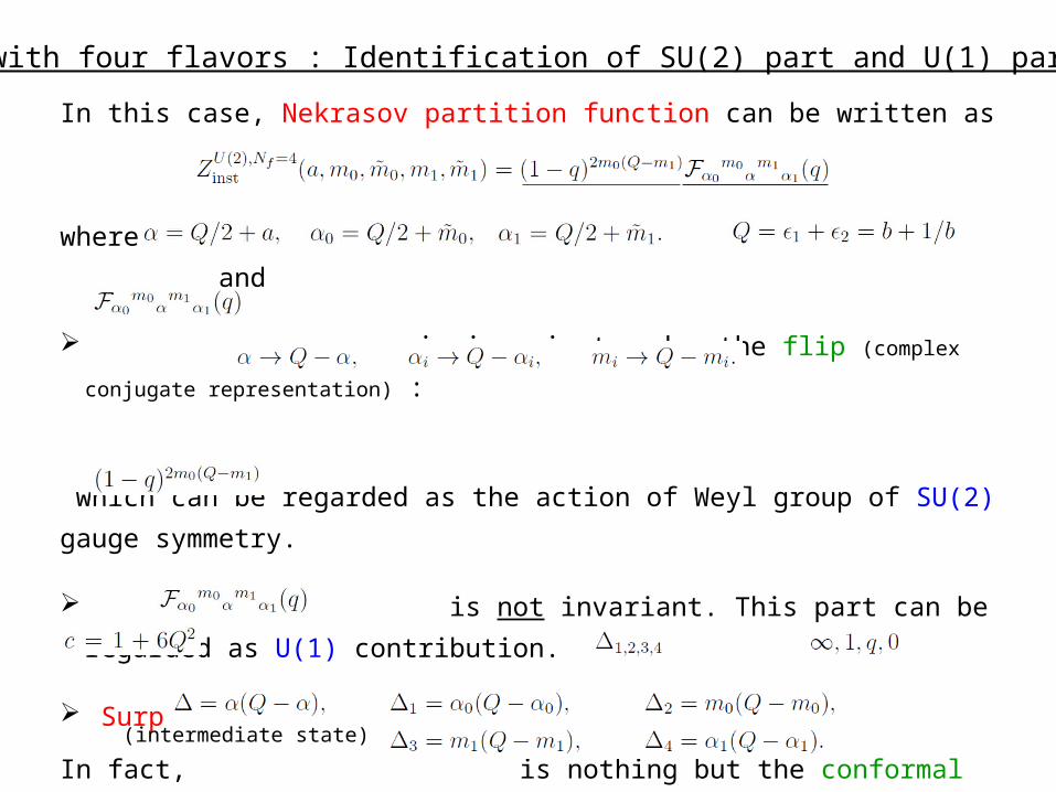
In this case, Nekrasov partition function can be written as

where and

is invariant under the flip (complex conjugate representation) :

which can be regarded as the action of Weyl group of SU(2) gauge

symmetry.

is not invariant. This part can be regarded as U(1)

contribution.

Surprising discovery by Alday-Gaiotto-Tachikawa

In fact, is nothing but the conformal block of Virasoro

algebra with

for four operators of dimensions inserted at :

SU(2) with four flavors : Identification of SU(2) part and U(1) part

(intermediate state)

Correlation function of Liouville theory with 　　　　　　 .

Thus, we naturally choose the primary vertex operator

as the examples of such operators. Then the 4-point function on a

sphere is

3-point function conformal block

where

The point is that we can make it of the form of square of absolute

value!

… only if

… using the properties : and

Liouville correlation function

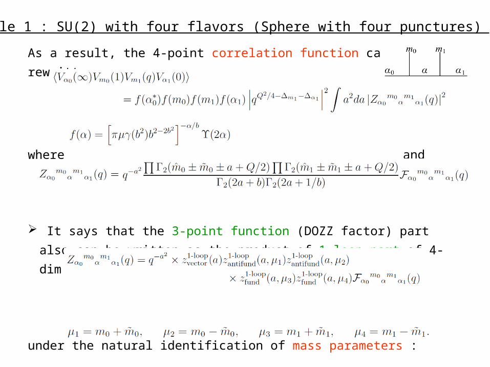
As a result, the 4-point correlation function can be rewritten as

where and

It says that the 3-point function (DOZZ factor) part also can be

written as the product of 1-loop part of 4-dim SU(2) partition

function :

under the natural identification of mass parameters :

Example 1 : SU(2) with four flavors (Sphere with four punctures)

Example 2 : Torus with one puncture

The SW curve in this case corresponds to 4-dim N=2* theory :

N=4 SU(2) theory deformed by a mass for the adjoint hypermultiplet

Nekrasov instanton partition function

This can be written as

where equals to the conformal block of Virasoro algebra with

Liouville correlation function (corresponding 1-point function)

where is Nekrasov’s partition

function.

Example 3 : Sphere with multiple punctures

The Seiberg-Witten curve in this case corresponds to

4-dim N=2 linear quiver SU(2) gauge theory.

Nekrasov instanton partition function

where equals to the conformal block of

Virasoro algebra with for the vertex operators which are

inserted at z=

Liouville correlation function (corresponding n+3-point function)

where is Nekrasov’s full partition function.

(↑ including 1-loop part)

U(1) part

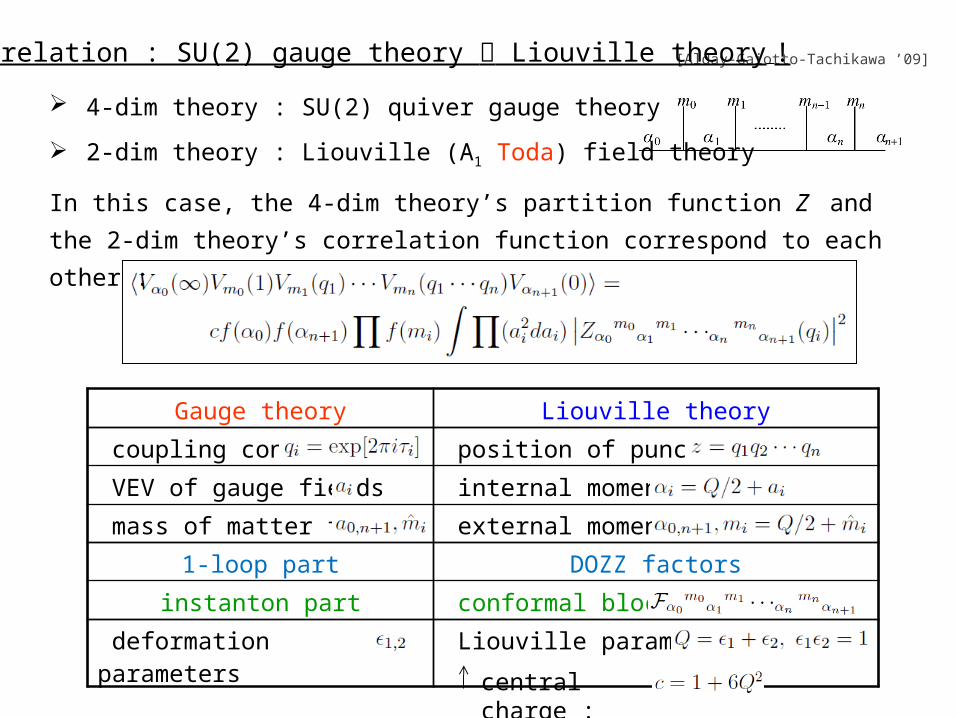
[Alday-Gaiotto-Tachikawa ’09]AGT relation : SU(2) gauge theory Liouville theory !

Gauge theory Liouville theory

coupling const. position of punctures

VEV of gauge fields internal momenta

mass of matter fields external momenta

1-loop part DOZZ factors

instanton part conformal blocks

deformation parameters Liouville parameters

4-dim theory : SU(2) quiver gauge theory

2-dim theory : Liouville (A1 Toda) field theory

In this case, the 4-dim theory’s partition function Z and the 2-dim

theory’s correlation function correspond to each other :

central charge :

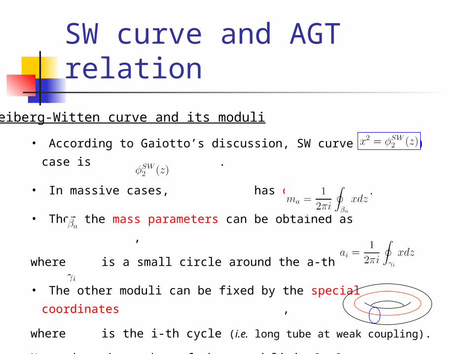
• According to Gaiotto’s discussion, SW curve for SU(2) case is

.

• In massive cases, has double poles.

• Then the mass parameters can be obtained as ,

where is a small circle around the a-th puncture.

• The other moduli can be fixed by the special coordinates

,

where is the i-th cycle (i.e. long tube at weak coupling).

Note that the number of these moduli is 3g-3+n. (g : # of genus, n : # of punctures)

SW curve and AGT relation

Seiberg-Witten curve and its moduli

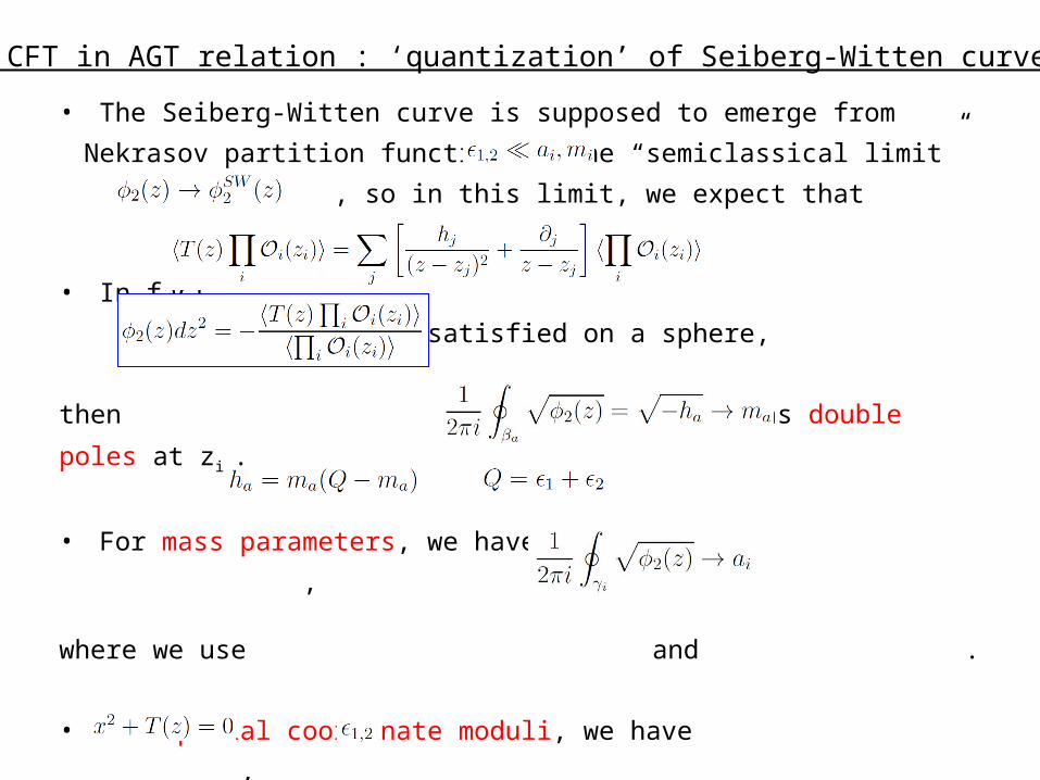
• The Seiberg-Witten curve is supposed to emerge from Nekrasov

partition function in the “semiclassical limit” , so in this

limit, we expect that .

• In fact, is satisfied on a

sphere,

then has double poles at zi .

• For mass parameters, we have ,

where we use and .

• For special coordinate moduli, we have ,

which can be checked by order by order calculation in concrete

examples.

• Therefore, it is natural to speculate that Seiberg-Witten curve is

‘quantized’ to at finite .

2-dim CFT in AGT relation : ‘quantization’ of Seiberg-Witten curve??

AGT-W relation for SU(N)

Now we calculate Nekrasov’s partition function of 4-dim SU(N) quiver

gauge theory as the quantity of interest.

SU(2) case : We consider only SU(2)×…×SU(2) quiver gauge

theories.

SU(N) case : According to Gaiotto’s discussion, we consider, in

general, the

cases of SU(d1) x SU(d2) x … x SU(N) x … x SU(N) x … x SU(d’2) x

SU(d’1) group,

where is non-negative.

SU(N) partition function

Nekrasov’s partition function of 4-dim gauge theory

xx xxx

*

… …x

*

…

…

…

d’3 – d’2d’2 – d’1d’1

… ………

…

d3 – d2

d2 – d1

d1… ………

1-loop part of partition function of 4-dim quiver gauge theory

We can obtain it of the analytic

form :

where each factor is defined as

: each factor is a product of double Gamma function!

,

gauge antifund. bifund. fund.

mass massmassflavor symm. of bifund. is U(1)

VEV# of d.o.f. depends on dk

deformation parameters

We obtain it of the expansion form of instanton

number :

where : coupling const. and

and

Instanton part of partition function of 4-dim quiver gauge theory

Young tableau

< Young tableau >

instanton # = # of boxes

leg

arm

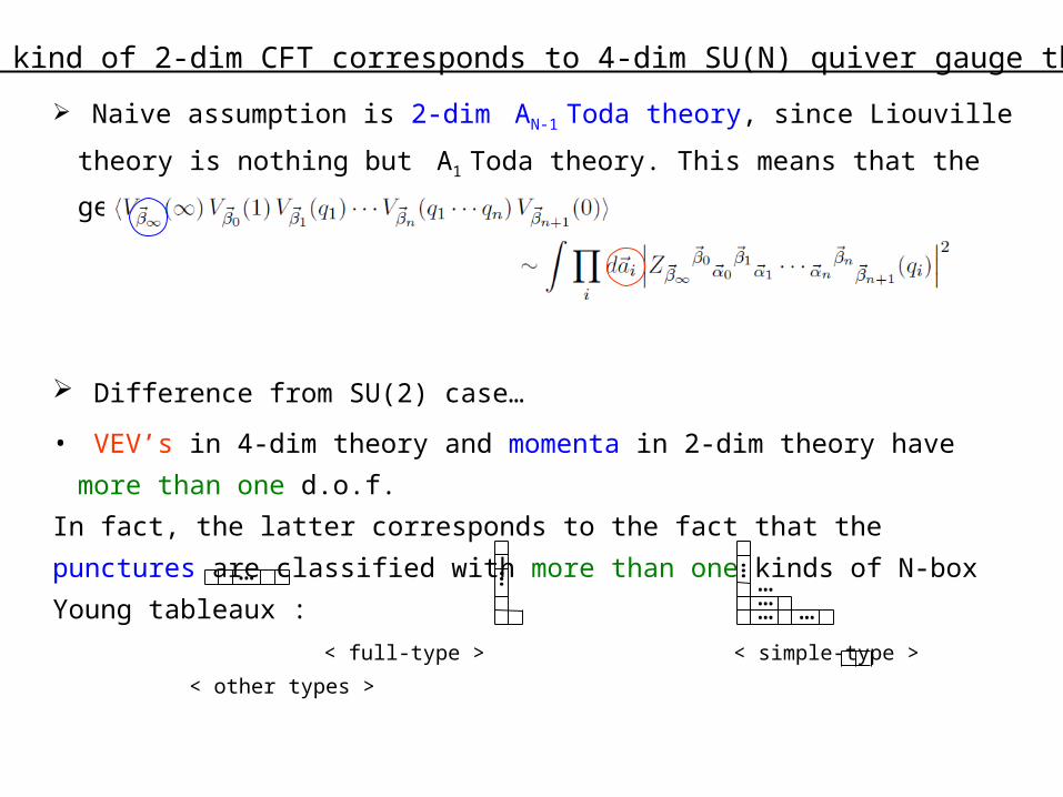
Naive assumption is 2-dim AN-1 Toda theory, since Liouville theory is

nothing but A1 Toda theory. This means that the generalized AGT

relation seems

Difference from SU(2) case…

• VEV’s in 4-dim theory and momenta in 2-dim theory have more than

one d.o.f.

In fact, the latter corresponds to the fact that the punctures are

classified with more than one kinds of N-box Young tableaux :

< full-type > < simple-type > < other types >

(cf. In SU(2) case, all these Young tableaux become ones of the same type .)

• In general, we don’t know how to calculate the conformal blocks of

Toda theory.

……

…

…

………

What kind of 2-dim CFT corresponds to 4-dim SU(N) quiver gauge theory?

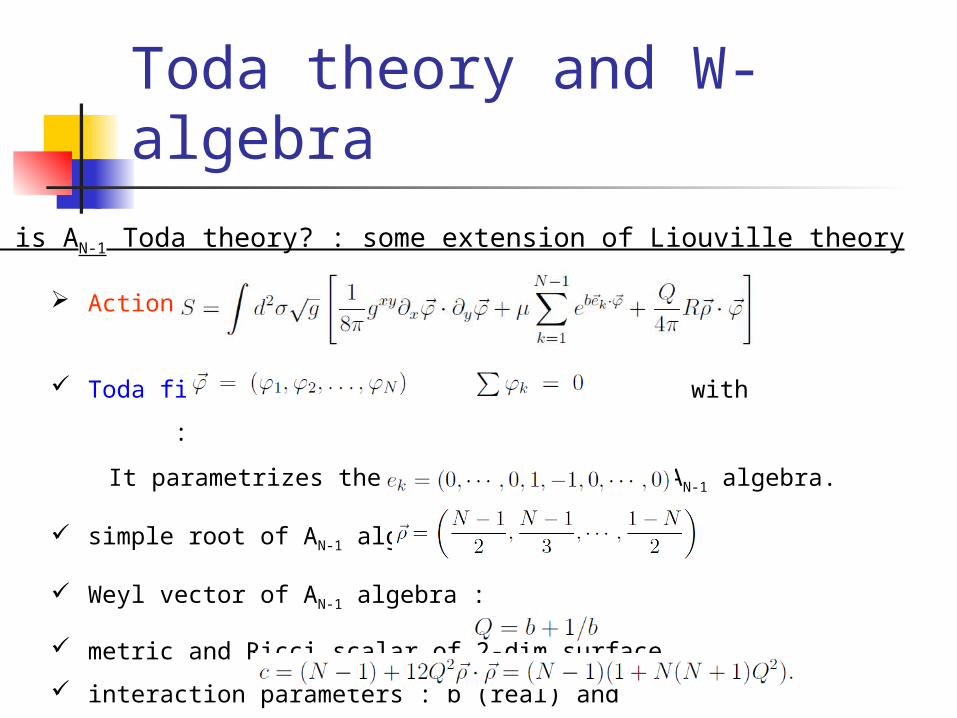
Action :

Toda field with :

It parametrizes the Cartan subspace of AN-1 algebra.

simple root of AN-1 algebra :

Weyl vector of AN-1 algebra :

metric and Ricci scalar of 2-dim surface

interaction parameters : b (real) and

central charge :

Toda theory and W-algebra

What is AN-1 Toda theory? : some extension of Liouville theory

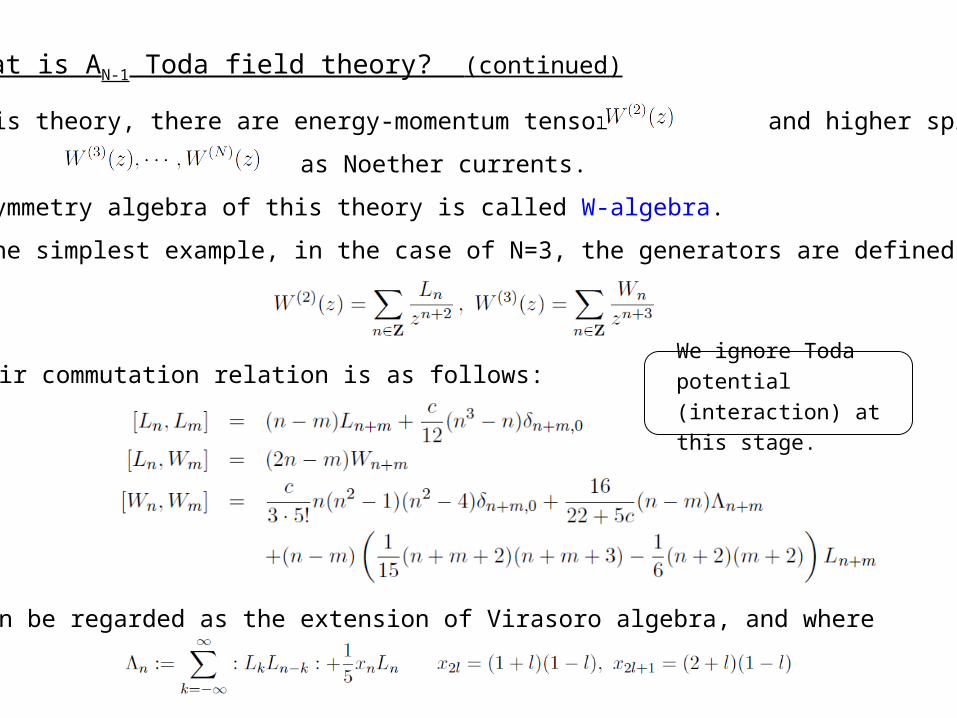
• In this theory, there are energy-momentum tensor and higher spin fields

as Noether currents.

• The symmetry algebra of this theory is called W-algebra.

• For the simplest example, in the case of N=3, the generators are defined as

And, their commutation relation is as follows:

which can be regarded as the extension of Virasoro algebra, and where

　　　　　　 ,

What is AN-1 Toda field theory? (continued)

We ignore Toda potential

(interaction) at this stage.

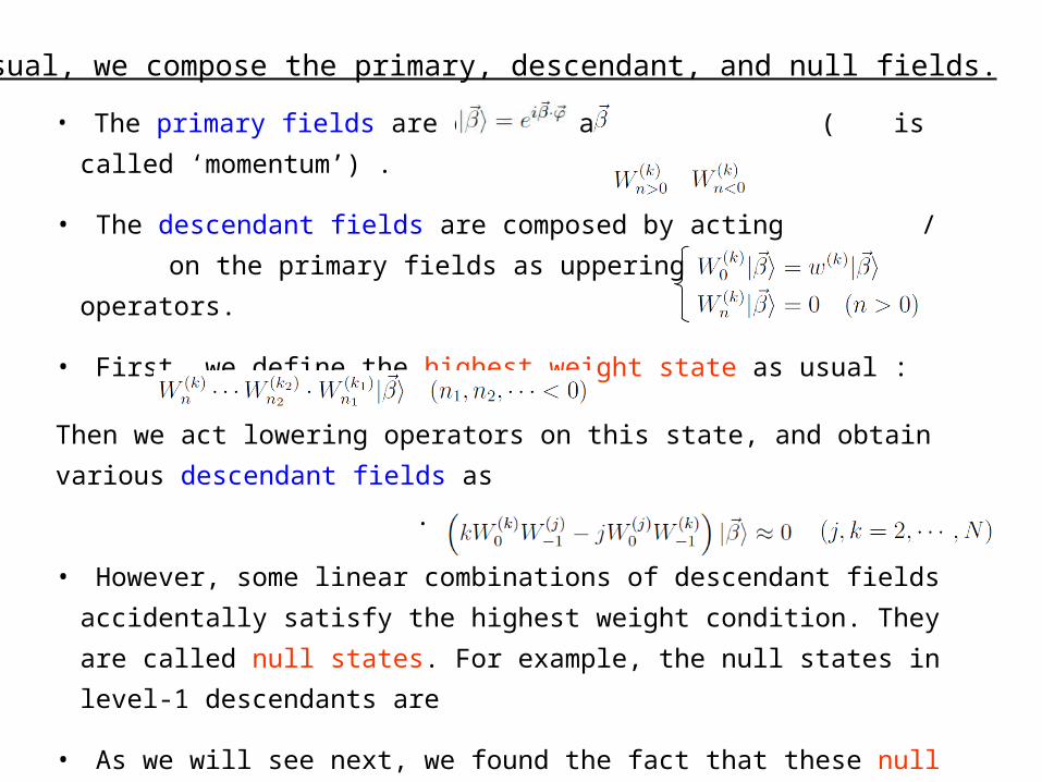
• The primary fields are defined as 　　　　　　　 ( is called

‘momentum’) .

• The descendant fields are composed by acting / 　 on the

primary fields as uppering / lowering operators.

• First, we define the highest weight state as usual :

Then we act lowering operators on this state, and obtain various

descendant fields as .

• However, some linear combinations of descendant fields

accidentally satisfy the highest weight condition. They are called

null states. For example, the null states in level-1 descendants are

• As we will see next, we found the fact that these null states in W-

algebra are closely related to the singular behavior of Seiberg-

Witten curve near the punctures. That is, Toda fields whose

existence is predicted by AGT relation may in fact describe the form

(or behavior) of Seiberg-Witten curve.

As usual, we compose the primary, descendant, and null fields.

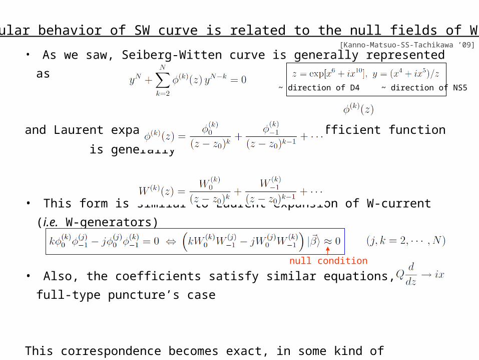
• As we saw, Seiberg-Witten curve is generally represented as

and Laurent expansion near z=z0 of the coefficient function is

generally

• This form is similar to Laurent expansion of W-current (i.e. W-

generators)

• Also, the coefficients satisfy similar equations, except full-type

puncture’s case

This correspondence becomes exact, in some kind of ‘classical’ limit:(which is related to Dijkgraaf-Vafa’s discussion on free fermion’s system?)

• This fact strongly suggests that vertex operators corresponding non-

full-type punctures must be the primary fields which has null states

in their descendants.

The singular behavior of SW curve is related to the null fields of W-algebra.[Kanno-Matsuo-SS-Tachikawa ’09]

null condition

~ direction of D4 　 ~ direction of NS5

• If we believe this suggestion, we can conjecture the form of

momentum of Toda field in vertex

operators , which corresponds to each kind of punctures.

• To find the form of vertex operators which have the level-1 null state,

it is useful to consider the screening operator (a special type of

vertex operator)

• We can show that the state satisfies the highest

weight condition, since the screening operator commutes with all the

W-generators.(Note a strange form of a ket, since the screening operator itself has non-zero

momentum.)

• This state doesn’t vanish, if the momentum satisfies

for some j. In this case, the vertex operator has a null state at level

.

The punctures on SW curve corresponds to the ‘degenerate’ fields![Kanno-Matsuo-SS-Tachikawa ’09]

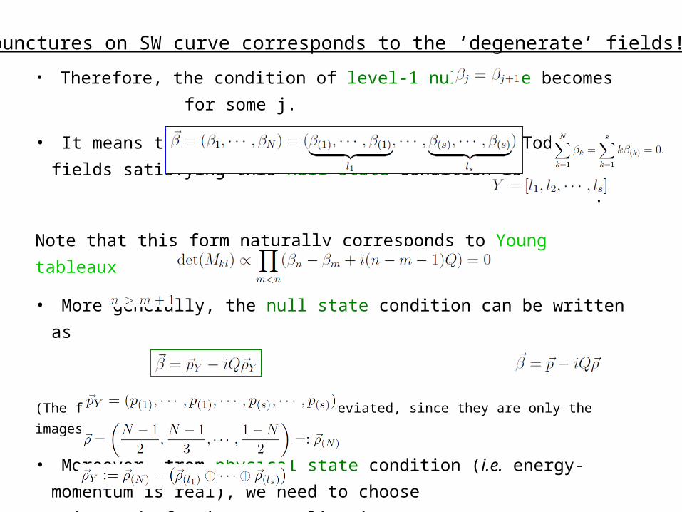
• Therefore, the condition of level-1 null state becomes for

some j.

• It means that the general form of mometum of Toda fields

satisfying this null state condition is

.

Note that this form naturally corresponds to Young tableaux

.

• More generally, the null state condition can be written as

(The factors are abbreviated, since they are only the images under Weyl

transformation.)

• Moreover, from physical state condition (i.e. energy-momentum is

real), we need to choose , instead of naive

generalization:

Here, is the same form of β,

is Weyl vector,

and .

The punctures on SW curve corresponds to the ‘degenerate’ fields!

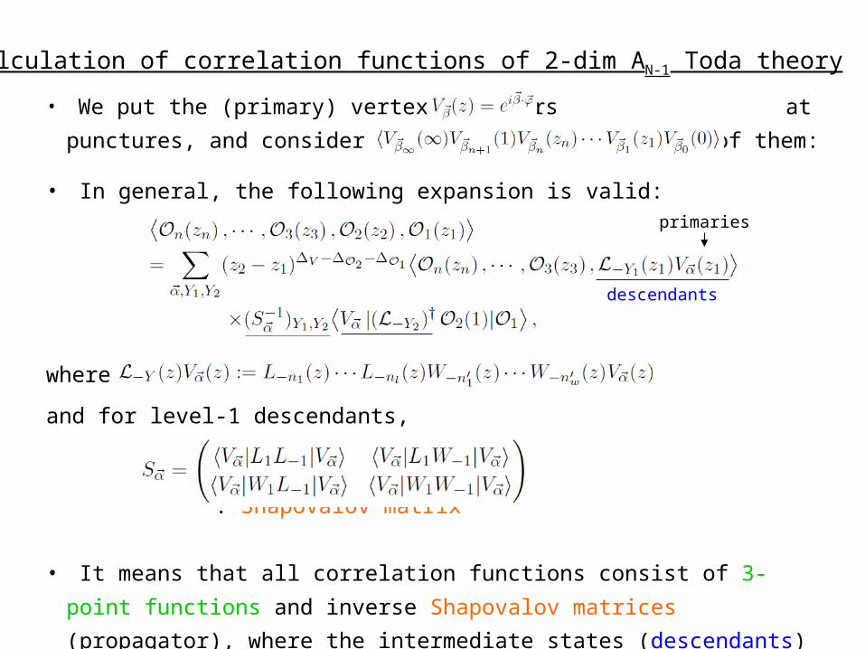
• We put the (primary) vertex operators at punctures, and

consider the correlation functions of them:

• In general, the following expansion is valid:

where

and for level-1 descendants,

: Shapovalov matrix

• It means that all correlation functions consist of 3-point functions

and inverse Shapovalov matrices (propagator), where the

intermediate states (descendants) can be classified by Young

tableaux.

On calculation of correlation functions of 2-dim AN-1 Toda theory

descendants

primaries

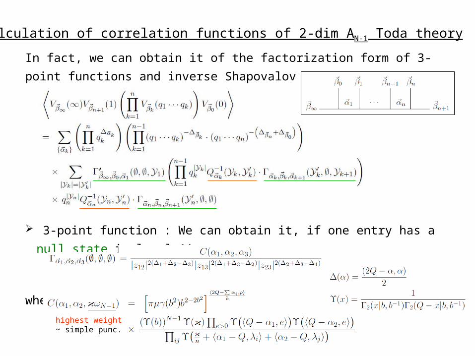
In fact, we can obtain it of the factorization form of 3-point functions

and inverse Shapovalov matrices :

3-point function : We can obtain it, if one entry has a null state in

level-1!

where

highest weight~ simple punc.

On calculation of correlation functions of 2-dim AN-1 Toda theory

’

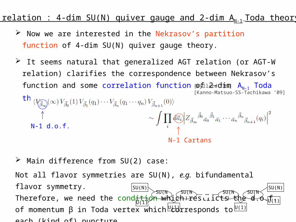
Now we are interested in the Nekrasov’s partition function of 4-dim

SU(N) quiver gauge theory.

It seems natural that generalized AGT relation (or AGT-W relation)

clarifies the correspondence between Nekrasov’s function and some

correlation function of 2-dim AN-1 Toda theory:

Main difference from SU(2) case:

Not all flavor symmetries are SU(N), e.g. bifundamental flavor

symmetry.

Therefore, we need the condition which restricts the d.o.f. of

momentum β in Toda vertex which corresponds to

each (kind of) puncture.

→ level-1 null state condition

[Wyllard ’09][Kanno-Matsuo-SS-Tachikawa ’09]

N-1 Cartans

SU(N)

SU(N)

SU(N)

U(1)

SU(N)

U(1) U(1)

SU(N)U(1)

SU(N)…

N-1 d.o.f.

AGT relation : 4-dim SU(N) quiver gauge and 2-dim AN-1 Toda theory

Correspondence between each kind of punctures and vertices

:

we conjectured it, using level-1 null state condition for non-full-type

punctures.

• full-type : correponds to SU(N) flavor symmetry (N-

1 d.o.f.)

• simple-type : corresponds to U(1) flavor symmetry (1 d.o.f.)

• other types : corresponds to other flavor symmetry

The corresponding momentum is of the form

which naturally corresponds to Young tableaux .

More precisely, the momentum is , where

[Kanno-Matsuo-SS-Tachikawa ’09]

…

…

…

…

………

Level-1 null state condition resolves the problems of AGT-W relation.

Difficulty for calculation of conformal blocks :

Here we consider the case of A2 Toda theory and W3-algebra. In usual,

the conformal blocks are written as the linear combination of

which cannot be determined by recursion formula.

However, in this case, thanks to the level-1 null state condition

we can completely determine all the conformal blocks.

Also, thanks to the level-1 null state condition, the 3-point function of

primary vertex fields can be determined completely:

Level-1 null state condition resolves the problems of AGT-W relation.

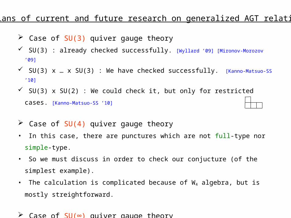
Case of SU(3) quiver gauge theory

SU(3) : already checked successfully. [Wyllard ’09] [Mironov-Morozov ’09]

SU(3) x … x SU(3) : We have checked successfully. [Kanno-Matsuo-SS ’10]

SU(3) x SU(2) : We could check it, but only for restricted cases. [Kanno-Matsuo-

SS ’10]

Case of SU(4) quiver gauge theory

• In this case, there are punctures which are not full-type nor simple-type.

• So we must discuss in order to check our conjucture (of the simplest

example).

• The calculation is complicated because of W4 algebra, but is mostly

streightforward.

Case of SU(∞) quiver gauge theory

• In this case, we consider the system of infinitely many M5-branes, which

may relate to AdS dual system of 11-dim supergravity.

• AdS dual system is already discussed using LLM’s droplet ansatz, which is

also governed by Toda equation. [Gaiotto-Maldacena ’09] →

subject of next section…

Our plans of current and future research on generalized AGT relation

AdS/CFT of AGT’s system

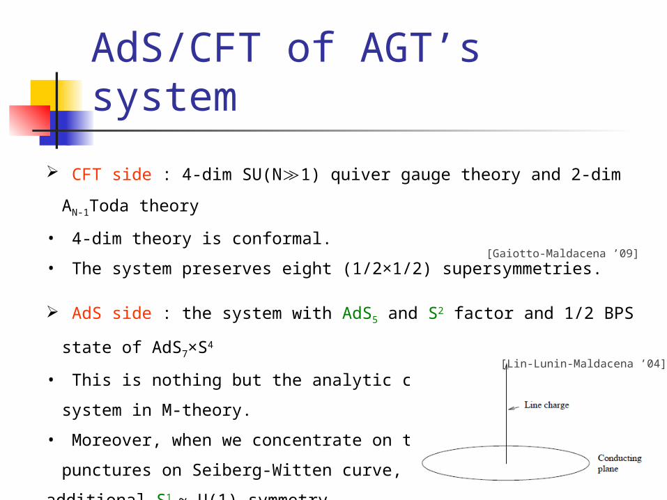
AdS/CFT of AGT’s system

CFT side : 4-dim SU(N≫1) quiver gauge theory and 2-dim AN-1Toda

theory

• 4-dim theory is conformal.

• The system preserves eight (1/2×1/2) supersymmetries.

AdS side : the system with AdS5 and S2 factor and 1/2 BPS state of

AdS7×S4

• This is nothing but the analytic continuation of LLM’s system in M-

theory.

• Moreover, when we concentrate on the neighborhood of punctures

on Seiberg-Witten curve, the system gets the

additional S1 ~ U(1) symmetry.

• According to LLM’s discussion, such system can

be analyzed using 3-dim electricity system:

[Gaiotto-Maldacena ’09]

[Lin-Lunin-Maldacena ’04]

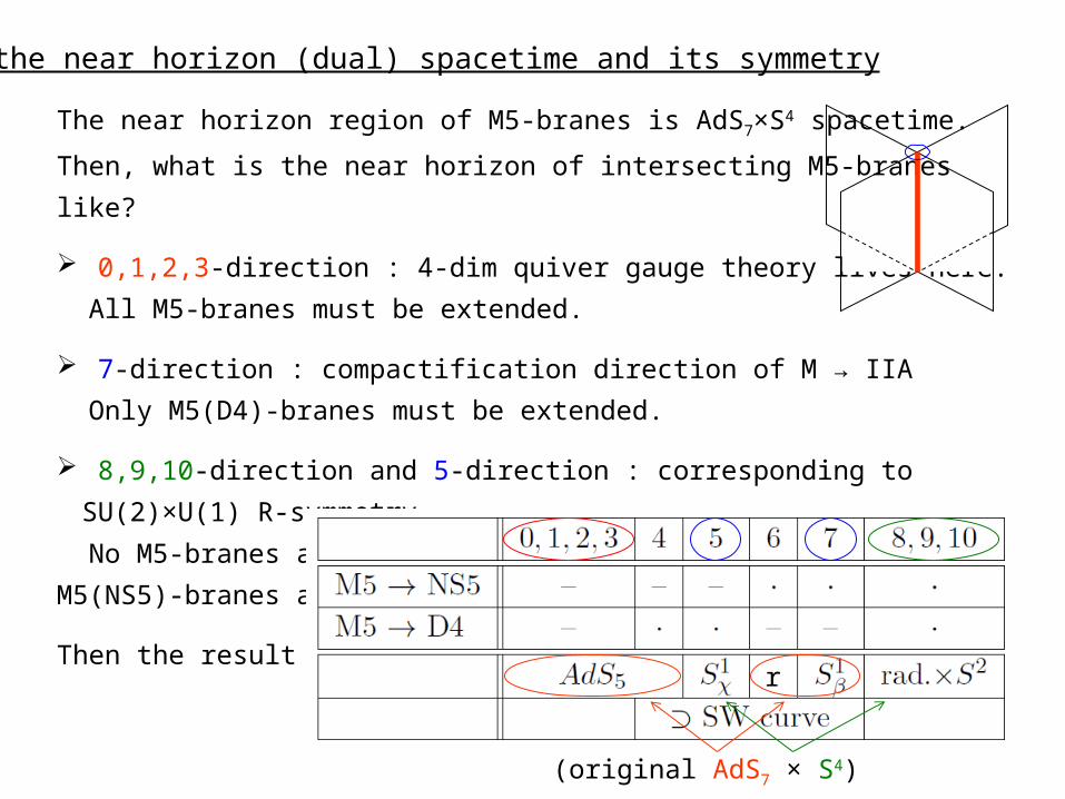
On the near horizon (dual) spacetime and its symmetry

The near horizon region of M5-branes is AdS7×S4 spacetime.

Then, what is the near horizon of intersecting M5-branes like?

0,1,2,3-direction : 4-dim quiver gauge theory lives here.

All M5-branes must be extended.

7-direction : compactification direction of M → IIA

Only M5(D4)-branes must be extended.

8,9,10-direction and 5-direction : corresponding to SU(2)×U(1) R-

symmetry

No M5-branes are extended to the former, and only M5(NS5)-branes

are to the latter.

Then the result is …

(original AdS7 × S4)

r

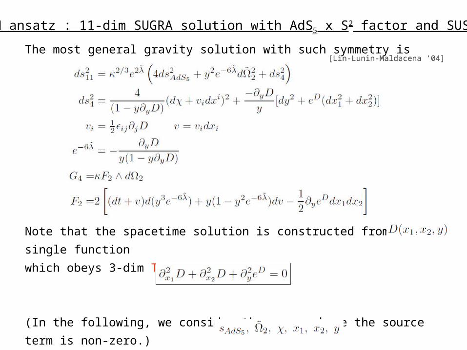
The most general gravity solution with such symmetry is

Note that the spacetime solution is constructed from a single

function

which obeys 3-dim Toda equation

(In the following, we consider the cases where the source term is

non-zero.)

cf. coordinates of 11-dim spacetime:

LLM ansatz : 11-dim SUGRA solution with AdS5 x S2 factor and SUSYs

[Lin-Lunin-Maldacena ’04]

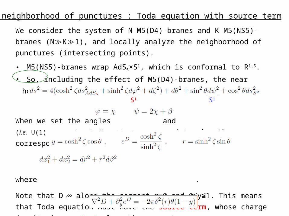
The neighborhood of punctures : Toda equation with source term

We consider the system of N M5(D4)-branes and K M5(NS5)-branes

(N≫K≫1), and locally analyze the neighborhood of punctures

(intersecting points).

• M5(NS5)-branes wrap AdS5×S1, which is conformal to R1,5.

• So, including the effect of M5(D4)-branes, the near horizon

geometry is also AdS7×S4 :

When we set the angles and (i.e. U(1) symm. for β-

direction), we can determine the correspondence to LLM ansatz

coordinates as

where .

Note that D→∞ along the segment r=0 and 0≦y≦1. This means that

Toda equation must have the source term, whose charge density is

constant along the segment:

S1 S1

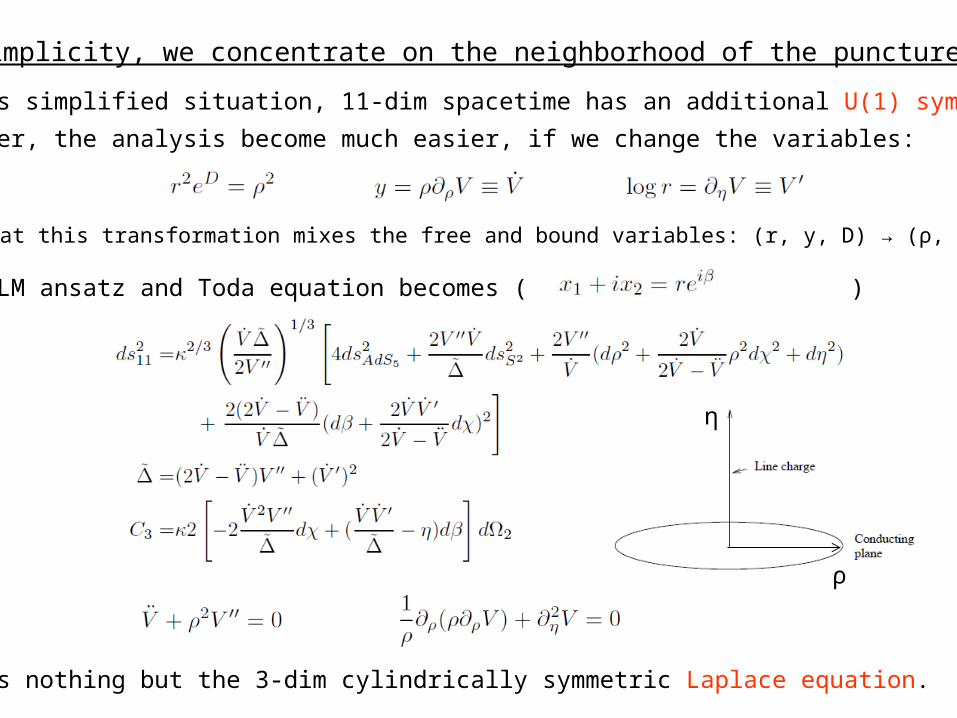
In this simplified situation, 11-dim spacetime has an additional U(1) symmetry.

Moreover, the analysis become much easier, if we change the variables:

Note that this transformation mixes the free and bound variables: (r, y, D) → (ρ, η, V)…

Then LLM ansatz and Toda equation becomes ( )

and

i.e.

This is nothing but the 3-dim cylindrically symmetric Laplace equation.

For simplicity, we concentrate on the neighborhood of the punctures.

ρ

η

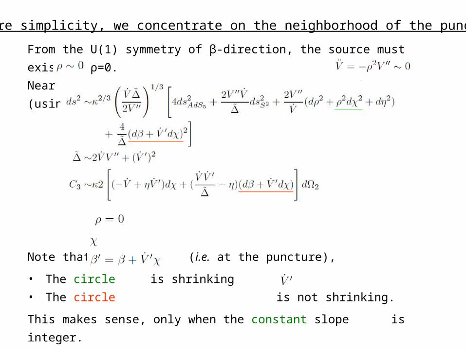
From the U(1) symmetry of β-direction, the source must exist at

ρ=0.

Near , LLM ansatz becomes more simple form (using

)

Note that at (i.e. at the puncture),

• The circle is shrinking

• The circle is not shrinking.

This makes sense, only when the constant slope is integer.

In fact, this integer slopes correspond to the size of quiver gauge

groups.(→ the next page…)

For more simplicity, we concentrate on the neighborhood of the punctures.

The neighborhood of punctures : Laplace equation with source term

We consider the such distribution of source charge:

When the slope is 1, we get smooth geometry.

When the slope is k, which corresponds to the

rescale and ,

we get Ak-1 singularity at and ,

since the period of β becomes .

In general, if the slope changes by k units, we get Ak-1 singularity there.

This can be regard the flavor symmetry of

additional k fundamental hypermultiplets.

This means the source charge corresponds to

nothing but the size of quiver gauge group.

N

Near , the potential can be written as (since ,

)

Then we obtain

,

So the boundary condition (~ source at r=0) is

On the source term : AdS/CFT correspondence for AGT relation !

integer

x*

x

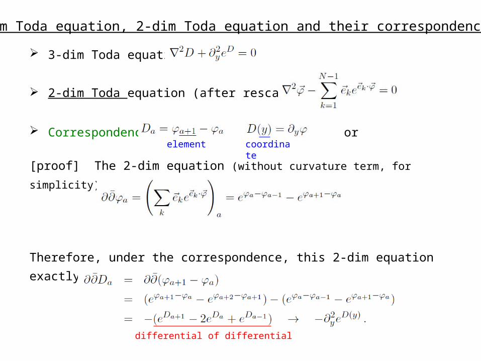
3-dim Toda equation, 2-dim Toda equation and their correspondence

3-dim Toda equation :

2-dim Toda equation (after rescaling of μ) :

Correspondence : or

[proof] The 2-dim equation (without curvature term, for simplicity) says

Therefore, under the correspondence, this 2-dim equation exactly

becomes the 3-dim equation:

differential of differential

element coordinate

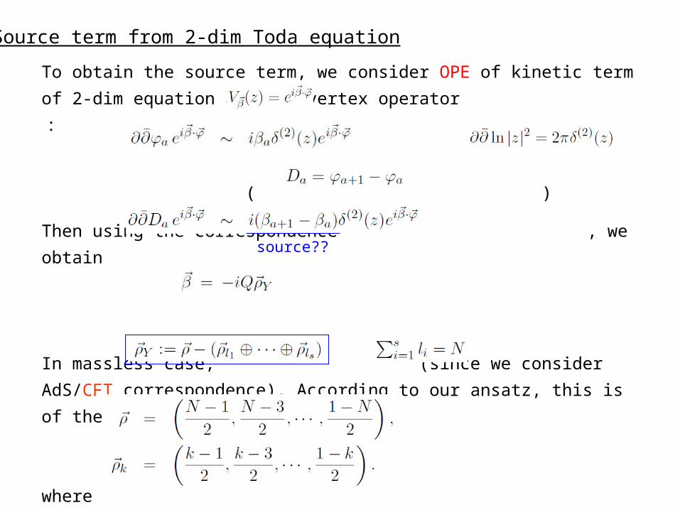
To obtain the source term, we consider OPE of kinetic term of 2-dim

equation and the vertex operator :

( )

Then using the correspondence , we obtain

In massless case, (since we consider AdS/CFT

correspondence). According to our ansatz, this is of the form

where

: N elements (Weyl

vector)

: k elements

Source term from 2-dim Toda equation

source??

Towards the correspondence of “source” in AdS/CFT context…?

• For full [1,…,1]-type puncture:

• For simple [N-1,1]-type puncture :

• For [l1,l2,…]-type puncture :

Conclusion

AGT relation reveals the interesting correspondence between 4-

dim N=2 linear or necklace SU(2) quiver gauge theory and 2-dim

Liouville theory.

We show (in part) that AGT-W relation for 4-dim linear SU(3)

quiver gauge theory and 2-dim A2 Toda theory is satisfied, by

checking 1-loop factor and some lower levels of instanton factor.

Here we use effectively the level-1 null state condition for vertices

in Toda theory.

As one way to study AGT-W relation for SU(N≫1) quiver gauge

theory, it can be useful to discuss AdS/CFT correspondence. Our

conjecture for general vertices in Toda theory enables us to study

this correspondence. This will be an important future work.