AND PROCEDURES GUIDE - Ohio State University · Your progress report on “Earthquake ... ranging from collaboration with NASA scientists or giving a seminar, ... (radar,"laser,"lidar),"synthetic"aperture"radar

Chunli DAI1

1 Division of Geodetic Science, School of Earth Sciences, The Ohio State Univ.

March 28, 2013 SMD/Earth Science Division Ms. Chunli Dai Division of Geodetic Science Ohio State University Columbus, OH 43210 Dear Ms. Dai: Thank you for your renewal application to the NASA Earth and Space Science Fellowship (NESSF) Program. Your progress report on “Earthquake Seismic Deformation From Spaceborne Gravimetry” (13-EARTH13R-76) is satisfactory, and has been approved for renewal. Attached is a copy of the updated NASA Earth and Space Science Fellowship Guide. This document contains information that you will find useful throughout the course of your fellowship. Please keep it handy for reference. Through a survey of previous graduates awarded with the NESSF grants, we have learned about the desire of many who would like to have the opportunity to visit NASA Centers. The reasons vary, ranging from collaboration with NASA scientists or giving a seminar, to job searching. The desired length of the visits also vary, ranging from days or a few weeks, to a full summer. If you have such a desire, we encourage you to familiarize yourself with the research and development undertaken by the various Centers. If we can help you or facilitate such a visit, please let Dr. Ming Ying Wei know by telephone (202) 358-0771 or via email at [email protected]. Upon receipt of your Ph.D. degree, you may wish to consider applying to the NASA Postdoctoral Program (NPP). The NPP offers unique research opportunities to highly talented national and international individuals to engage in ongoing NASA research programs at a NASA Center. These fellowship appointments, one to three years in duration, are competitive and are designed to advance NASA's goals and objectives. The NPP is administered for NASA by Oak Ridge Associated Universities. You will find more detailed information by visiting the NPP website at http://nasa.orau.org/postdoc/.

THE NATIONAL SCIENCE FOUNDATION

PROPOSAL AWARD POLICIES

AND

AND

PROCEDURES GUIDE

OCTOBER 2012 EFFECTIVE JANUARY 14, 2013NSF 13-1OMB Control Number: 3145-0058

Supported by:

A SCIENCE DISCIPLINE TO STUDY THE EARTH’S (PLANETS’) SIZE (GRAVITY), SHAPE (VOLUME), AND THEIR CHANGES; AND TO DETERMINE THE POSITION, VELOCITY AND FOR TIME-TRANSFER OF A POINT ANYWHERE ON EARTH’S SURFACE OR IN SPACE!

WHAT IS GEODESY?!

http://geodeticscience.osu.edu!http://geodeticscience.org!

NASA, ESA, CNES, JAXA

CONTEMPORARY GEODETIC SATELLITES

ALEX BRAUN

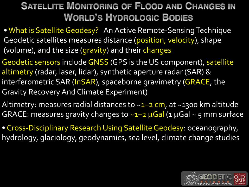
•"What"is"Satellite"Geodesy?"""An"Active"Remote7Sensing"Technique"Geodetic"satellites"measures"distance"(position,"velocity),"shape"(volume),"and"the"size"(gravity)"and"their"changes"Geodetic"sensors"include"GNSS"(GPS"is"the"US"component),"satellite"altimetry"(radar,"laser,"lidar),"synthetic"aperture"radar"(SAR)"&"interferometric"SAR"(InSAR),"spaceborne"gravimetry"(GRACE,"the"Gravity"Recovery"And"Climate"Experiment)"

•"Cross7Disciplinary"Research"Using"Satellite"Geodesy:"oceanography,"hydrology,"glaciology,"geodynamics,"sea"level,"climate"change"studies"

Altimetry:"measures"radial"distances"to"~1–2"cm,"at"~1300"km"altitude"GRACE:"measures"gravity"changes"to"~1–2"µGal"(1"µGal"~"5"mm"surface"

* Bangladesh*Sea,Level*Coastal*Vulnerability**

4"

Not to scale

Schematic Credit: Steven Tseng, Ohio State Univ.

Not to scale

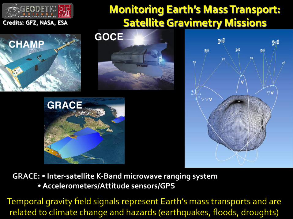
Monitoring"Earth’s"Mass"Transport:"Satellite"Gravimetry"Missions"

CHAMP GOCE

GRACE

GRACE:"•"Inter>satellite"K>Band"microwave"ranging"system""""""""""""""""•"Accelerometers/Attitude"sensors/GPS"

Temporal"gravity"field"signals"represent"Earth’s"mass"transports"and"are"related"to"climate"change"and"hazards"(earthquakes,"floods,"droughts)"

Credits: GFZ, NASA, ESA

6"

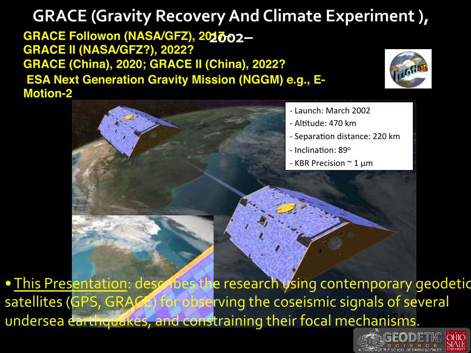
GRACE"(Gravity"Recovery"And"Climate"Experiment"),"2002–"

!"Launch:"March"2002"! "Al0tude:"470"km"! "Separa0on"distance:"220"km"! "Inclina0on:"89o"

! "KBR"Precision"~"1"μm*

NASA

GRACE Followon (NASA/GFZ), 2017– GRACE II (NASA/GFZ?), 2022? GRACE (China), 2020; GRACE II (China), 2022?

!

ESA Next Generation Gravity Mission (NGGM) e.g., E-Motion-2

•"This"Presentation:"describes"the"research"using"contemporary"geodetic"satellites"(GPS,"GRACE)"for"observing"the"coseismic"signals"of"several"undersea"earthquakes,"and"constraining"their"focal"mechanisms."

* 

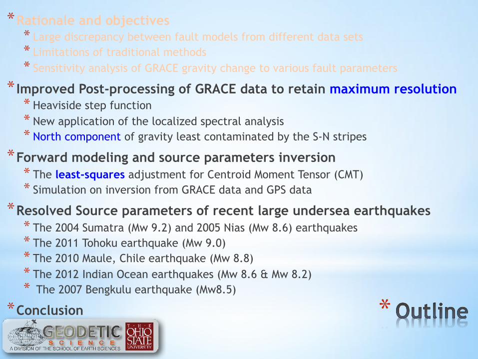
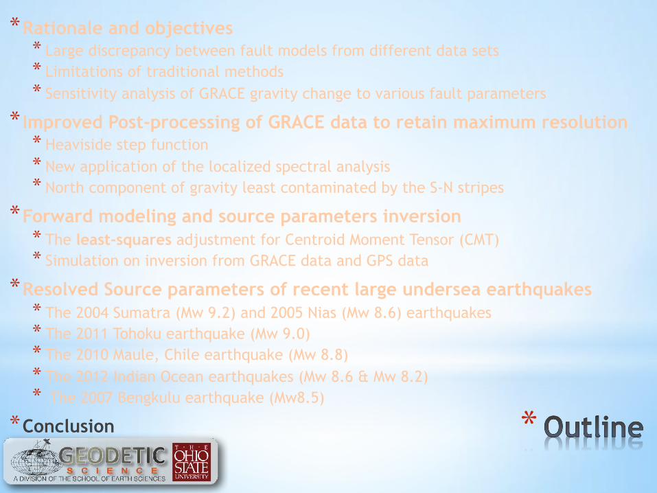
* Rationale and objectives * Large discrepancy between fault models from different data sets * Limitations of traditional methods * Sensitivity analysis of GRACE gravity change to various fault parameters

* Improved Post-processing of GRACE data to retain maximum resolution * Heaviside step function * New application of the localized spectral analysis * North component of gravity least contaminated by the S-N stripes

* Forward modeling and source parameters inversion * The least-squares adjustment for Centroid Moment Tensor (CMT) * Simulation on inversion from GRACE data and GPS data

* Resolved Source parameters of recent large undersea earthquakes * The 2004 Sumatra (Mw 9.2) and 2005 Nias (Mw 8.6) earthquakes * The 2011 Tohoku earthquake (Mw 9.0) * The 2010 Maule, Chile earthquake (Mw 8.8) * The 2012 Indian Ocean earthquakes (Mw 8.6 & Mw 8.2) * The 2007 Bengkulu earthquake (Mw8.5)

* Conclusion

* 

* Traditional methods on solving for source parameters and their limitations * Seismological data * Difficulty for rupture with long duration due to the overlap of interfering

arrivals [Lay et al., 2005; Bilek et al., 2007; Chlieh et al., 2007]

* Shortcomings for detecting slow or aseismic slip and postseismic slip [Chlieh et al., 2007; Han et al., 2013]

* Sensitive to waveform types and the frequency band

* Highly dependent on the velocity structure

* GPS data, Interferometric Synthetic Aperture Radar (InSAR) data, vertical displacements on coral reefs, Repeated airborne LiDAR data * Limited by the spatial distribution of the observations

* Tsunami data

* 

* How can GRACE measure the earthquakes signal?

10 µGal = 10-8 g

Mass redistribution caused by earthquakes

* 

* Hypothesis: by surveying right above the fault area, GRACE can better constrain the centroid location and slip orientation, with our new approach for GRACE data processing with no filter.

* Recent studies of estimating source parameters using GRACE data * Based on finite fault model [Cambiotti and Sabadini, 2012; Wang

et al., 2012a, 2012b; Dai et al., 2014] * Based on Centroid Moment Tensor [Han et al., 2011, 2013;

Cambiotti and Sabadini, 2013].

* This study * emphasizes the use of the north component of the gravity change * achieves enhanced resolutions, using higher degree solutions * applies the localized spectral analysis [Wieczorek & Simons, 2005]

to determine the practical spherical harmonic truncation degree * solves for CMT, using the least-squares adjustment considering the

linear algorithm between coseismic gravity change and CMT

http://www.gps.alaska.edu

* 

Trade-off between strike and rake angle [Han et al., 2011, 2013; Dai et al., 2014]

Acknowledge Prof. Jeff Freymueller

* 




* Resolved Source parameters of recent large undersea earthquakes * The 2004 Sumatra (Mw 9.2) and 2005 Nias (Mw 8.6) earthquakes * The 2011 Tohoku earthquake (Mw 9.0) * The 2010 Maule, Chile earthquake (Mw 8.8) * The 2012 Indian Ocean earthquakes (Mw 8.6 & Mw 8.2) *  The 2007 Bengkulu earthquake (Mw8.5)

* Conclusion

Time series on the grid point (140.2°E 36.85°N). The red line is the fitting value using the annual, semiannual, 161-days periods, and the Heaviside step function. CSR RL05 high degree monthly gravity solution (NMAX 96), used to derive gravity and gravity gradient disturbance time series up to degree 70§

140.2°E(36.85°N(

* 

gN

Txx

Comparison to other

methods:

1.  Subtracting gravity change before and after the earthquake [Han et al., 2006, 2010, 2011] -> deficiency on reducing random noise

2.  Utilizing Slepian functions [Wang et al., 2012a, 2012b] ->not a rigorous representation

§Updated from Dai et al. GRL [2014]

* GRACE measured inter-satellite K/Ka-band range acceleration is directly driven by the gravity vector difference projected to the line of sight direction which is mostly north-south direction

12ρ!!

112 ge !!⋅ 212 ge !!

⋅gN = −

1r∂T∂θ

Txx (r,θ,λ) = 1r

Tr (r,θ,λ)+ 1r2 Tθθ (r,θ,λ)

Txy (r,θ,λ) = Tyx (r,θ,λ) = 1r2 sinθ

−cotθTλ (r,θ,λ)+Tθλ (r,θ,λ)( )

Txz (r,θ,λ) = Tzx (r,θ,λ) = 1r2 Tθ (r,θ,λ)− 1

rTrθ (r,θ,λ) x, y, z direction: North, West, Up

* 

* 





* Conclusion

* 

* CMT M = I3 =determinant (M)= 0

* M for a shear fault can be expressed by the strike, dip, rake angle, and the seismic moment, M0

! The linear relationship between gravity change and moment tensor

= [B1, B2, B3, B4, B5]

M xx M xy M xz

M xy M yy M yz

M xz M yz Mzz

!

"

####

$

%

&&&&

M xx +M yy +Mzz = 0

TnDiDD

ngggy ]......[ ,,1,

1=

×

ξ5×1= M xx M xy M xz M yz Mzz"#$

%&'

T

ξ5×1

yn×1

Acknowledge Dr. Junyi Guo

* 

* To be consistent with GRACE-observed gravity and gravity gradient change 1.  The gravity change are evaluated at the ocean floor using

Wang’s PSGRN/PSCMP software [Wang et al., 2006, Courtesy, R. Wang].

2.  Evaluate the effect of ocean response [de Linage et al., 2009; Cambiotti et al., 2011; Li and Chen, 2013; Broerse et al., 2014]. σ = −H ×ρw ×OF


12km

30~60% of the solid Earth gravity increase

* 

* To be consistent with GRACE-observed gravity and gravity gradient change 1.  The gravity change are evaluated at the ocean floor using

Wang’s PSGRN/PSCMP software [Wang et al., 2006, Courtesy, R. Wang].

2.  Evaluate the effect of ocean response [de Linage et al., 2009; Cambiotti et al., 2011; Li and Chen, 2013; Broerse et al., 2014].

3.  Gravity change due to solid earth deformation and surface density change at ocean floor is transformed to SH coefficients up to degree 899.

4.  gN, Txx computed on Earth’s mean semi-major axis (6378.1363 km) from SH coefficients up to degree 70.

* Difference of the gravity evaluated on the ocean floor and on Earth’s semi-major axis can be significant, e.g., causing the magnitude to drop for about 40% for the 2011 Tohoku earthquake, but it has not been discussed in many previous publications

σ = −H ×ρw ×OF


* 

* Observation equation

With fixed constraint I3=0 :

=0

* To find the optimal centroid location and depth, adopt the simulated annealing algorithm. Target function is:

yI4n1×1

= AI4n1×5

ξ5×1+ eI

4n1×1

M xxM yyMzz + 2M xyM xzM yz −M xxM yz2 −M yyM xz

2 −MzzM xy2

Φ lat, lon, depth( ) = rdgN+ rdTxx

+ rdTxy+ rdTxz( ) / 4

* 

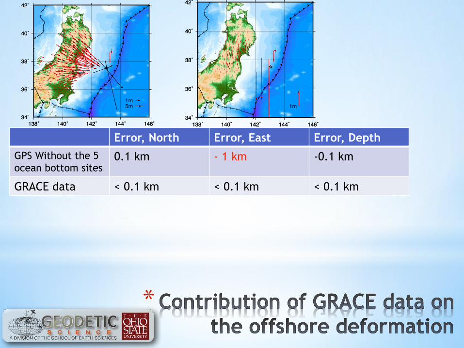
Error, North Error, East Error, Depth

GPS Without the 5 ocean bottom sites

0.1 km - 1 km -0.1 km

GRACE data < 0.1 km < 0.1 km < 0.1 km

138˚ 140˚ 142˚ 144˚ 146˚34˚

36˚

38˚

40˚

42˚

138˚ 140˚ 142˚ 144˚ 146˚34˚

36˚

38˚

40˚

42˚

1m5m

138˚ 140˚ 142˚ 144˚ 146˚34˚

36˚

38˚

40˚

42˚

138˚ 140˚ 142˚ 144˚ 146˚34˚

36˚

38˚

40˚

42˚

1m

* 





* Conclusion

* 

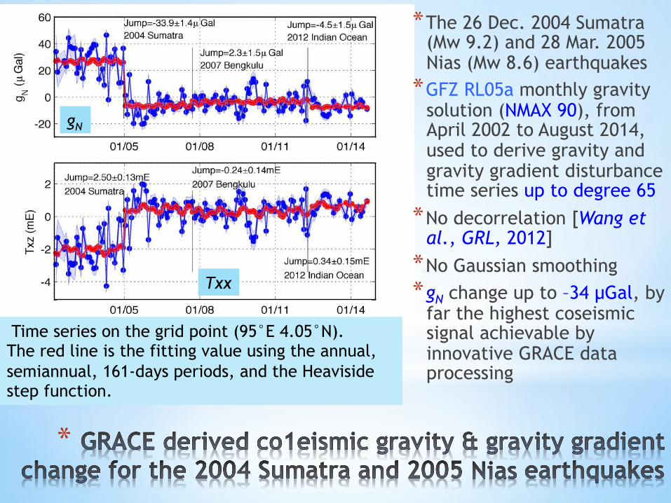
Time series on the grid point (95°E 4.05°N). The red line is the fitting value using the annual, semiannual, 161-days periods, and the Heaviside step function.

gN

Txx

* The 26 Dec. 2004 Sumatra (Mw 9.2) and 28 Mar. 2005 Nias (Mw 8.6) earthquakes * GFZ RL05a monthly gravity

solution (NMAX 90), from April 2002 to August 2014, used to derive gravity and gravity gradient disturbance time series up to degree 65

* No decorrelation [Wang et al., GRL, 2012] * No Gaussian smoothing * gN change up to –34 µGal, by

far the highest coseismic signal achievable by innovative GRACE data processing

140˚ 141˚ 142˚ 143˚ 144˚ 145˚35˚

36˚

37˚

38˚

39˚

40˚

41˚

140˚ 141˚ 142˚ 143˚ 144˚ 145˚35˚

36˚

37˚

38˚

39˚

40˚

41˚

09

182736

(m)

*  Finite Fault: the rake angle, fault location, width, and average slip

*  Slip orientation about 8° clockwise of GCMT, consistent with observation by GOCE [Fuchs et al., 2013]

*  Location and slip azimuth consistent for two GRACE products and two inversion scheme

* 

Model name Data Sources Centroid Strike (°)

Dip (°) Rake (°)

Slip azimuth (°)

Seismic Moment [Nm]

Wei et al., 2012 Ozawa et al., 2011

GPS and Seismic data

Blue beach ball 200 10 88 112 4.04×1022

GCMT Long-period mantle waves

Black beach ball 203 10 88 115 5.31×1022

USGS CMT Seismic data Green beach ball 187 14 68 120 4.5×1022

This study CSR RL05 N60 - 201* 10* 77 124 6.43×1022

This study CSR RL05 N96 Red beach ball 236 12 113 123 4.03×1022 Strike Dip Rake M0

Strike 1 0.4 1 0 Dip 0.4 1 0.2 0.1

Rake 1 0.2 1 0.1 M0 0 0.1 0.1 1

β = φs − arctan sinλ cosδ / cosλ( ) ≈ φs −λ

* GRACE data is able to provide additional constraint similar to the offshore GPS observation

* 

gN Txx Txy Txz CSR RMS 3.08 µGal 0.18 mE 0.15 mE 0.23 mE

CSR minus Model 1*

RMS 1.5 µGal 0.078 mE 0.086 mE 0.118 mE Relative difference 47.75% 43.72% 57.94% 50.42%

CSR minus Model 4§

RMS 1.6 µGal 0.093 mE 0.089 mE 0.131 mE Relative difference 53.11% 52.01% 60.19% 55.82%

Table 4.1. RMS and relative differences between the GRACE observation and two slip models predictions. *Model 1 is the slip model [Wang et al. 2013] determined using both onshore and offshore GPS/Acoustic Network data §Model 4 is the slip model [Wang et al. 2013] determined using only onshore GPS data

−76˚ −74˚ −72˚

−38˚

−36˚

−34˚

−32˚

−76˚ −74˚ −72˚

−38˚

−36˚

−34˚

−32˚

048

1216

(m)

*  GRACE-observed gN up to +10.6±1.3 µGal,

compared to gD change up to –8.0 µGal [Wang et al., 2012a]

* 

Strike (°) Dip (°) Rake (°) gN/gD 270 9 90 0.97 0 9 90 0.35 19 18 116 0.39

69.4°W'32.45°S'

* 

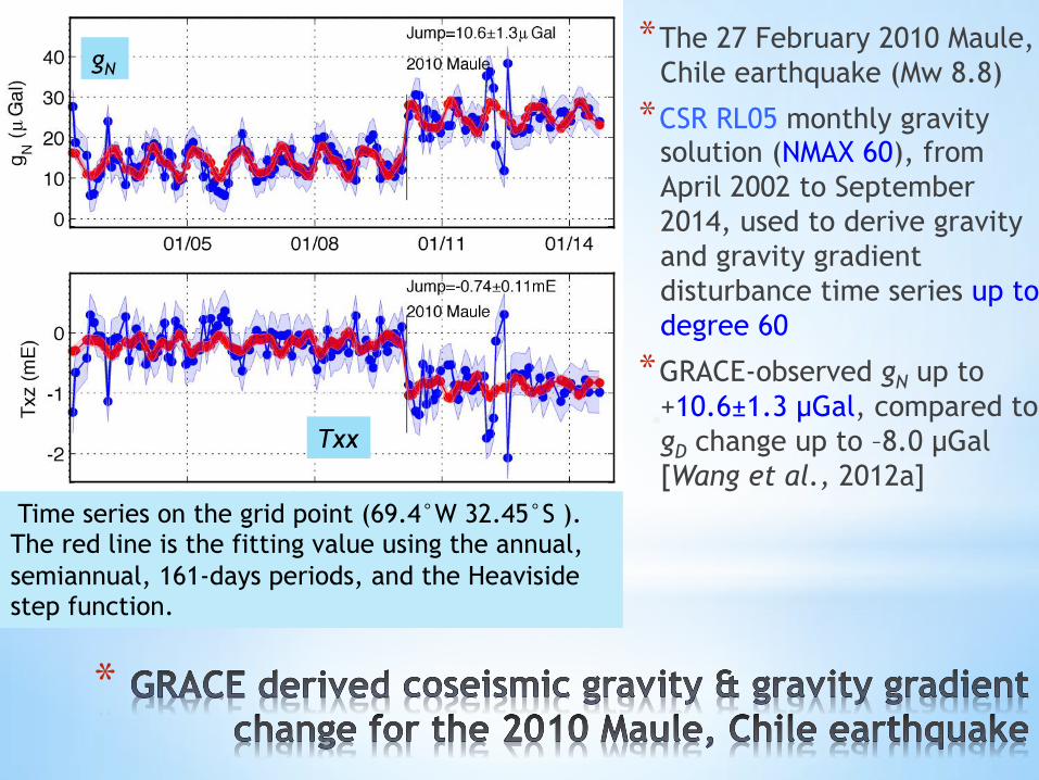
Time series on the grid point (69.4°W 32.45°S ). The red line is the fitting value using the annual, semiannual, 161-days periods, and the Heaviside step function.

gN

Txx

* The 27 February 2010 Maule, Chile earthquake (Mw 8.8)

* CSR RL05 monthly gravity solution (NMAX 60), from April 2002 to September 2014, used to derive gravity and gravity gradient disturbance time series up to degree 60

* GRACE-observed gN up to +10.6±1.3 µGal, compared to gD change up to –8.0 µGal [Wang et al., 2012a]

*  The 11 April 2012 Indian Ocean earthquakes (Mw 8.6 & Mw 8.2)

*  Geodetic constraints on the static fault geometry are limited

*  Debates about whether east-west right-lateral slips or meridian-aligned left-lateral slips

*  Vertical strike-slip earthquake indicating small gD change -> up to –5.7±0.7 µGal for gN and 0.26±0.03 mE for Txz

* 

RMS of the residual gN ( µGal) Txx (mE) Txy (mE) Txz (mE)

OSU 0.77 0.024 0.017 0.030

CSR RL05 0.76 0.024 0.017 0.032 CSR RL05* 0.88 0.030 0.018 0.037

GFZ RL05a 1.01 0.028 0.023 0.037

3.45%N%88.4%E%

* 

Time series on the grid point (88.4°E 3.45°N). The red line is the fitting value using the annual, semiannual, 161-days periods, and the Heaviside step function.

gN

Txx

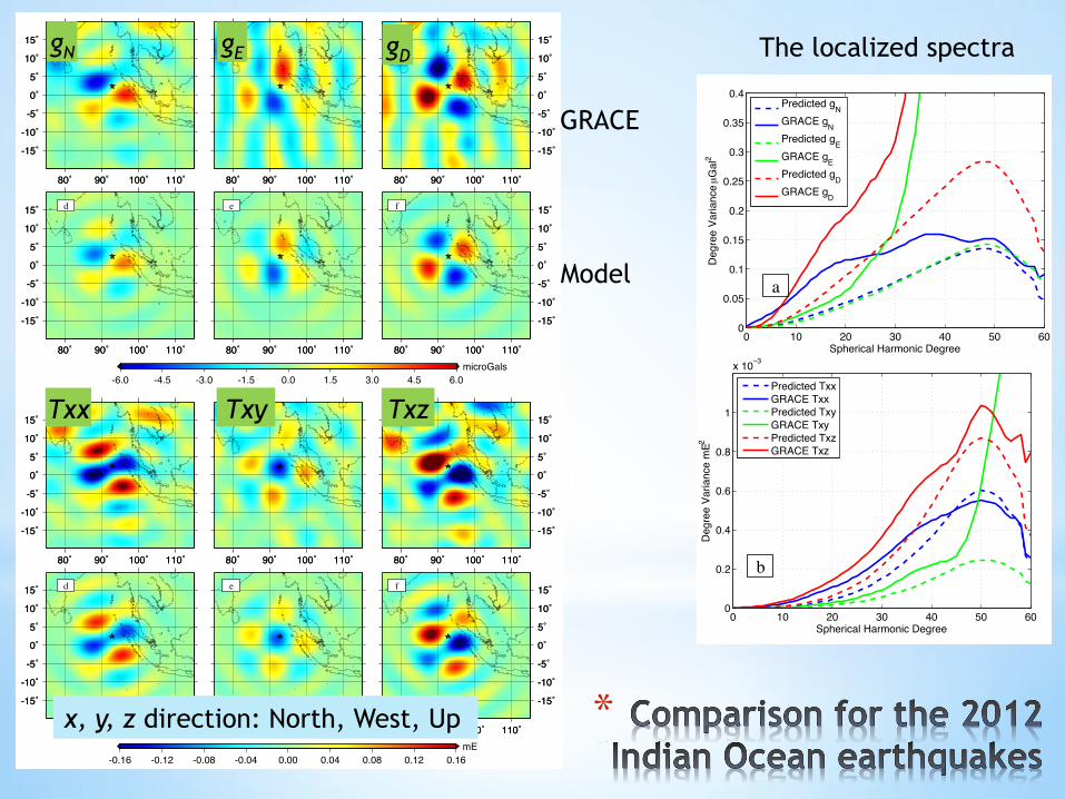
* The 11 April 2012 Indian Ocean earthquakes (Mw 8.6 & Mw 8.2)

* CSR RL05 monthly gravity solution (NMAX 60), from April 2002 to September 2014, used to derive gravity and gravity gradient disturbance time series up to degree 40

* No decorrelation [Wang et al., GRL, 2012]

* No Gaussian smoothing

0 10 20 30 40 50 600

0.2

0.4

0.6

0.8

1

x 10−3

Spherical Harmonic Degree

Deg

ree

Varia

nce

mE2

Predicted TxxGRACE TxxPredicted TxyGRACE TxyPredicted TxzGRACE Txz

0 10 20 30 40 50 600

0.05

0.1

0.15

0.2

0.25

0.3

0.35

0.4


Deg

ree

Varia

nce µ

Gal

2

Predicted gNGRACE gNPredicted gEGRACE gEPredicted gDGRACE gD

a b

0 10 20 30 40 50 600

0.2

0.4

0.6

0.8

1

x 10−3


Deg

ree

Varia

nce

mE2


0 10 20 30 40 50 600

0.05

0.1

0.15

0.2

0.25

0.3

0.35

0.4


Deg

ree

Varia

nce µ

Gal

2


a b

80˚ 90˚ 100˚ 110˚

-15˚

-10˚

-5˚

0˚

5˚

10˚

15˚

80˚ 90˚ 100˚ 110˚

-15˚

-10˚

-5˚

0˚

5˚

10˚

15˚

80˚ 90˚ 100˚ 110˚80˚ 90˚ 100˚ 110˚ 80˚ 90˚ 100˚ 110˚

-15˚

-10˚

-5˚

0˚

5˚

10˚

15˚

80˚ 90˚ 100˚ 110˚

-15˚

-10˚

-5˚

0˚

5˚

10˚

15˚

-0.16 -0.12 -0.08 -0.04 0.00 0.04 0.08 0.12 0.16mE

80˚ 90˚ 100˚ 110˚

-15˚

-10˚

-5˚

0˚

5˚

10˚

15˚

80˚ 90˚ 100˚ 110˚

-15˚

-10˚

-5˚

0˚

5˚

10˚

15˚

80˚ 90˚ 100˚ 110˚80˚ 90˚ 100˚ 110˚ 80˚ 90˚ 100˚ 110˚

-15˚

-10˚

-5˚

0˚

5˚

10˚

15˚

80˚ 90˚ 100˚ 110˚

-15˚

-10˚

-5˚

0˚

5˚

10˚

15˚

-0.16 -0.12 -0.08 -0.04 0.00 0.04 0.08 0.12 0.16mE

b a c b a c

d e f

80˚ 90˚ 100˚ 110˚

-15˚

-10˚

-5˚

0˚

5˚

10˚

15˚

80˚ 90˚ 100˚ 110˚

-15˚

-10˚

-5˚

0˚

5˚

10˚

15˚

80˚ 90˚ 100˚ 110˚80˚ 90˚ 100˚ 110˚ 80˚ 90˚ 100˚ 110˚

-15˚

-10˚

-5˚

0˚

5˚

10˚

15˚

80˚ 90˚ 100˚ 110˚

-15˚

-10˚

-5˚

0˚

5˚

10˚

15˚

-6.0 -4.5 -3.0 -1.5 0.0 1.5 3.0 4.5 6.0microGals

80˚ 90˚ 100˚ 110˚

-15˚

-10˚

-5˚

0˚

5˚

10˚

15˚

80˚ 90˚ 100˚ 110˚

-15˚

-10˚

-5˚

0˚

5˚

10˚

15˚

80˚ 90˚ 100˚ 110˚80˚ 90˚ 100˚ 110˚ 80˚ 90˚ 100˚ 110˚

-15˚

-10˚

-5˚

0˚

5˚

10˚

15˚

80˚ 90˚ 100˚ 110˚

-15˚

-10˚

-5˚

0˚

5˚

10˚

15˚

-6.0 -4.5 -3.0 -1.5 0.0 1.5 3.0 4.5 6.0microGals

b a c b a c

d e f

gN gE gD

Txy Txx Txz

The localized spectra

* 

GRACE

Model

x, y, z direction: North, West, Up

* 

RMS of the residual

gN (µGal)

Txx (mE)

Txy (mE)

Txz (mE)

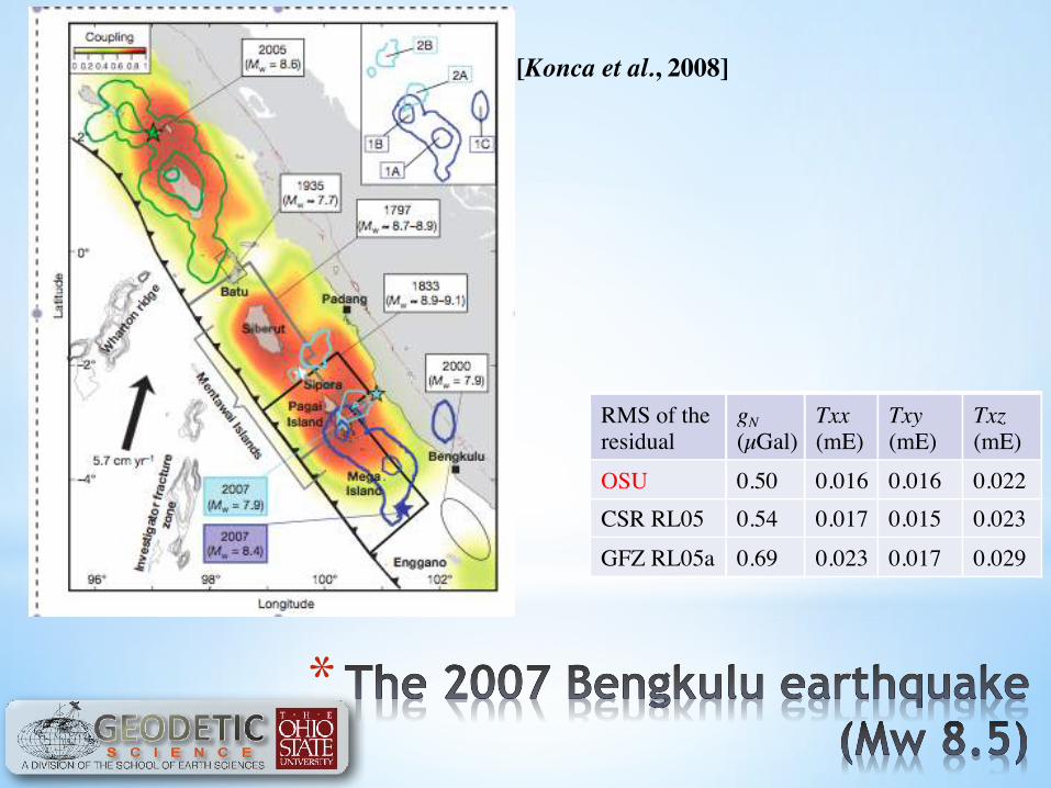
OSU 0.50 0.016 0.016 0.022 CSR RL05 0.54 0.017 0.015 0.023 GFZ RL05a 0.69 0.023 0.017 0.029

[Konca et al., 2008]

* 

Time series on the grid point (100.6°E 7.95°S). The red line is the fitting value using the annual, semiannual, 161-days periods, and the Heaviside step function.

gN

Txx

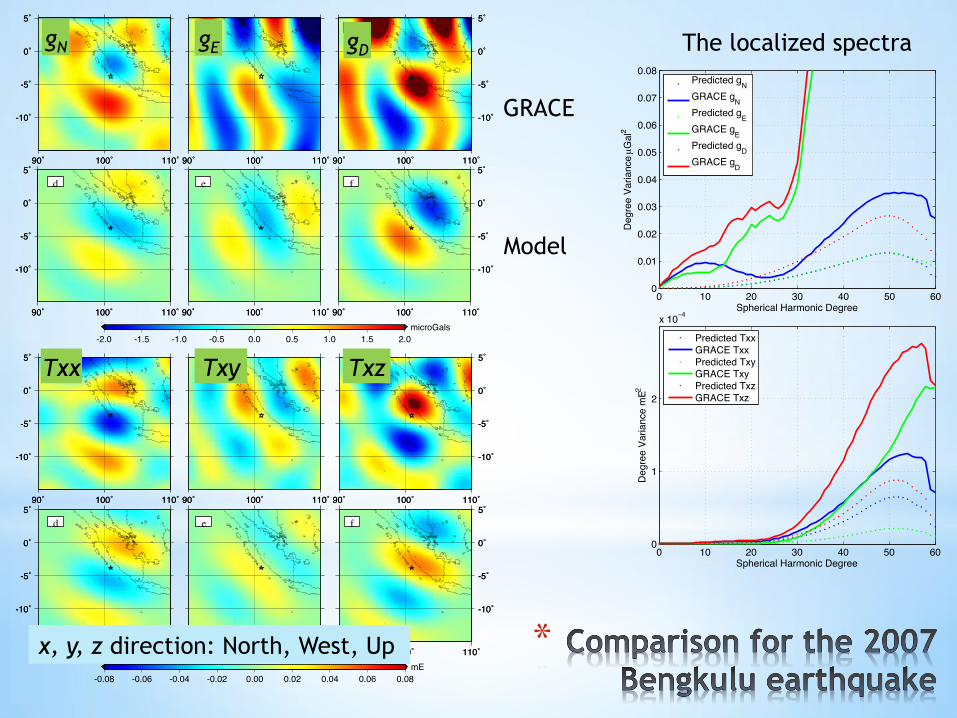
* The 12 September 2007 Bengkulu earthquake (Mw8.5) * OSU monthly gravity solution

(NMAX 60), from January 2003 to December 2013, based on energy method [Guo et al. 2014; Shang et al., 2014], used to derive gravity and gravity gradient disturbance time series up to degree 40

* No decorrelation [Wang et al., GRL, 2012] * No Gaussian smoothing

0 10 20 30 40 50 600

1

2

x 10−4


Deg

ree

Varia

nce

mE2


90˚ 100˚ 110˚

-10˚

-5˚

0˚

5˚

90˚ 100˚ 110˚

-10˚

-5˚

0˚

5˚

90˚ 100˚ 110˚90˚ 100˚ 110˚ 90˚ 100˚ 110˚

-10˚

-5˚

0˚

5˚

90˚ 100˚ 110˚

-10˚

-5˚

0˚

5˚

-2.0 -1.5 -1.0 -0.5 0.0 0.5 1.0 1.5 2.0microGals

90˚ 100˚ 110˚

-10˚

-5˚

0˚

5˚

90˚ 100˚ 110˚

-10˚

-5˚

0˚

5˚

90˚ 100˚ 110˚90˚ 100˚ 110˚ 90˚ 100˚ 110˚

-10˚

-5˚

0˚

5˚

90˚ 100˚ 110˚

-10˚

-5˚

0˚

5˚

-2.0 -1.5 -1.0 -0.5 0.0 0.5 1.0 1.5 2.0microGals

b a c

d e f

90˚ 100˚ 110˚

-10˚

-5˚

0˚

5˚

90˚ 100˚ 110˚

-10˚

-5˚

0˚

5˚

90˚ 100˚ 110˚90˚ 100˚ 110˚ 90˚ 100˚ 110˚

-10˚

-5˚

0˚

5˚

90˚ 100˚ 110˚

-10˚

-5˚

0˚

5˚

-0.08 -0.06 -0.04 -0.02 0.00 0.02 0.04 0.06 0.08mE

90˚ 100˚ 110˚

-10˚

-5˚

0˚

5˚

90˚ 100˚ 110˚

-10˚

-5˚

0˚

5˚

90˚ 100˚ 110˚90˚ 100˚ 110˚ 90˚ 100˚ 110˚

-10˚

-5˚

0˚

5˚

90˚ 100˚ 110˚

-10˚

-5˚

0˚

5˚

-0.08 -0.06 -0.04 -0.02 0.00 0.02 0.04 0.06 0.08mE

b a c

d e f

gN gE gD

Txy Txx Txz

The localized spectra

* 

0 10 20 30 40 50 600

0.01

0.02

0.03

0.04

0.05

0.06

0.07

0.08


Deg

ree

Varia

nce µ

Gal

2


GRACE

Model

x, y, z direction: North, West, Up

*  Slip direction about 14° counterclockwise w.r.t. GCMT; Konca et al.’s about 11° clockwise w.r.t. GCMT

*  Consider the trade-off [Kanamori and Given, 1981]

* 

M0 sin2δ

98˚ 100˚ 102˚ 104˚-6˚

-4˚

-2˚

0˚

98˚ 100˚ 102˚ 104˚-6˚

-4˚

-2˚

0˚

02468

(m)

* 





* Conclusion

* Conclusions

35"

•""Multiple"geodetic"satellites"are"abundant"and"measures"different"quantities"(water"level"and"mass"changes)"at"different"resolutions."""

•"The"improvement"of"measurement"precision"are"anticipated"for"GRACE7Followon"or"GRACE7II"missions"for"the"detecting"of"smaller"earthquakes."

•"Examples"provided"here"include"monitoring"the"focal"mechanisms"of"several"large"undersea"earthquakes"using"GRACE"gravimetry"

* 

* This research is primarily supported by NASA’s Earth and Space Science Fellowship (ESSF) Program (Grant NNX12AO06H), partially supported by National Science Foundation (NSF) Division of Earth Sciences (Grant EAR-1013333). * GRACE data products are from NASA’s PODAAC via Jet Propulsion

Laboratory/California Institute of Technology (JPL), University of Texas Center for Space Research (CSR), and GeoForschungsZentrum Potsdam (GFZ). * Preliminary GPS time series provided by the ARIA team at JPL

and Caltech. All original GEONET RINEX data were provided to California Institute of Technology by the Geospatial Information Authority (GSI) of Japan. * Some figures in this paper were generated using the Generic

Mapping Tools (GMT) [Wessel and Smith, 1991]. * This work was also supported in part by an allocation of

computing resources from the Ohio Supercomputer Center (http://www.osc.edu)

Thank you

* 

Strike Dip Rake M0

Strike 1 0.4 1 –0.4 Dip 0.4 1 0.5 –0.4

Rake 1 0.5 1 –0.6 M0 –0.4 –0.4 –0.6 1

Strike Dip Rake M0

Strike 1 0.4 1 0 Dip 0.4 1 0.2 0.1

Rake 1 0.2 1 0.1 M0 0 0.1 0.1 1

2004 Sumatra, dip 8~32

2011 Tohoku, dip 10~14

*  Explanation on why the strike and rake angles are correlated [Han et al., 2013] :

M xz ≈ −M0 cos φs −λ( ) M yz ≈ M0 sin λ −φs( ) M xy ≈ M0δ cos 2φs −λ( ) M yy −M xx ≈ 2M0δ sin(2φs −λ)


Strike, , dip, , rake angle, φs δ λ

Slip Direction:

* 

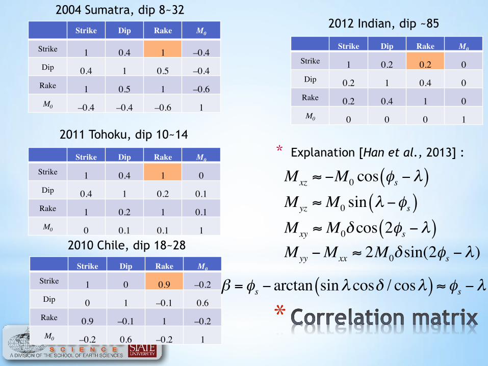
Strike Dip Rake M0

Strike 1 0.4 1 –0.4 Dip 0.4 1 0.5 –0.4

Rake 1 0.5 1 –0.6 M0 –0.4 –0.4 –0.6 1

Strike Dip Rake M0

Strike 1 0.2 0.2 0 Dip 0.2 1 0.4 0

Rake 0.2 0.4 1 0 M0 0 0 0 1

Strike Dip Rake M0

Strike 1 0 0.9 –0.2 Dip 0 1 –0.1 0.6

Rake 0.9 –0.1 1 –0.2 M0 –0.2 0.6 –0.2 1

Strike Dip Rake M0

Strike 1 0.4 1 0 Dip 0.4 1 0.2 0.1

Rake 1 0.2 1 0.1 M0 0 0.1 0.1 1

2004 Sumatra, dip 8~32

2011 Tohoku, dip 10~14

2010 Chile, dip 18~28

2012 Indian, dip ~85

*  Explanation [Han et al., 2013] :

M xz ≈ −M0 cos φs −λ( ) M yz ≈ M0 sin λ −φs( ) M xy ≈ M0δ cos 2φs −λ( ) M yy −M xx ≈ 2M0δ sin(2φs −λ)


* 

Error, North Error, East Error, Depth

GPS Without the 5 ocean bottom sites

0.1 km - 1 km -0.1 km

GRACE data < 0.1 km < 0.1 km < 0.1 km

138˚ 140˚ 142˚ 144˚ 146˚34˚

36˚

38˚

40˚

42˚

138˚ 140˚ 142˚ 144˚ 146˚34˚

36˚

38˚

40˚

42˚

1m5m

138˚ 140˚ 142˚ 144˚ 146˚34˚

36˚

38˚

40˚

42˚

138˚ 140˚ 142˚ 144˚ 146˚34˚

36˚

38˚

40˚

42˚

1m

GRACE only GPS only GPS and GRACE

Documents

AND PROCEDURES GUIDE - Ohio State University · Your progress report on “Earthquake ... ranging from collaboration with NASA scientists or giving a seminar, ... (radar,"laser,"lidar),"synthetic"aperture"radar