Embed Size (px)
Citation preview
arX
iv:1
906.
0032
6v1
[cs
.CC
] 2
Jun
201
9
Approximate degree, secret sharing, and concentration phenomena
Andrej Bogdanov1, Nikhil S. Mande2, Justin Thaler2, and Christopher Williamson1
andrejb, [email protected]
nikhil.mande, [email protected] University of Hong Kong
2Georgetown University
Abstract
The ε-approximate degree degε(f) of a Boolean function f is the least degree of a real-valued poly-
nomial that approximates f pointwise to within ε. A sound and complete certificate for approximate
degree being at least k is a pair of probability distributions, also known as a dual polynomial, that are
perfectly k-wise indistinguishable, but are distinguishable by f with advantage 1− ε. Our contributions
are:
• We give a simple, explicit new construction of a dual polynomial for the AND function on n bits,
certifying that its ε-approximate degree is Ω(√
n log 1/ε)
. This construction is the first to extend
to the notion of weighted degree, and yields the first explicit certificate that the 1/3-approximate
degree of any (possibly unbalanced) read-once DNF is Ω(√n). It draws a novel connection be-
tween the approximate degree of AND and anti-concentration of the Binomial distribution.
• We show that any pair of symmetric distributions on n-bit strings that are perfectly k-wise indis-
tinguishable are also statistically K-wise indistinguishable with at most K3/2 · exp(−Ω
(k2/K
))
error for all k < K ≤ n/64. This bound is essentially tight, and implies that any symmetric func-
tion f is a reconstruction function with constant advantage for a ramp secret sharing scheme that
is secure against size-K coalitions with statistical errorK3/2 ·exp(−Ω
(deg
1/3(f)2/K
))for all
values of K up to n/64 simultaneously. Previous secret sharing schemes required that K be de-
termined in advance, and only worked for f = AND. Our analysis draws another new connection
between approximate degree and concentration phenomena.
As a corollary of this result, we show that for any d ≤ n/64, any degree d polynomial approx-
imating a symmetric function f to error 1/3 must have coefficients of ℓ1-norm at least K−3/2 ·exp
(Ω(
deg1/3 (f)
2 /d))
. We also show this bound is essentially tight for any d > deg1/3(f).
These upper and lower bounds were also previously only known in the case f = AND.
1 Introduction
The ε-approximate degree of a function f : −1, 1n → 0, 1, denoted degε(f), is the least degree of a
multivariate real-valued polynomial p such that |p(x)− f(x)| ≤ ε for all inputs x ∈ −1, 1n.1 Such a p is
said to be an approximating polynomial for f . This is a central object of study in computational complexity,
owing to its polynomial equivalence to many other complexity measures including sensitivity, exact degree,
deterministic and randomized query complexity [21], and quantum query complexity [6].
By linear programming duality, f has ε-approximate degree more than k if and only if there exist a pair
of probability distributions µ and ν over the domain of f such that µ and ν are perfectly k-wise indistin-
guishable (i.e., all k-wise projections of µ and ν are identical), but are (1− ε)-distinguishable by f , namely
EX∼µ[f(X)]−EY∼ν [f(Y )] ≥ 1−ε. Said equivalently, a sound and complete certificate for ε-approximate
degree being more than k is a dual polynomial q = (µ − ν)/2 that contains no monomials of degree k or
less, and such that∑
x |q(x)| = 1 and∑
x q(x)f(x) ≥ ε.Dual polynomials have immediate applications to cryptographic secret sharing: a dual polynomial q =
(µ−ν)/2 for f is a description of a cryptographic scheme for sharing a 1-bit secret amongst n parties, where
the secret can be reconstructed by applying f to the shares, and the scheme is secure against coalitions of
size k (see [4] for details).
Motivation for explicit constructions of dual polynomials. Recent years have seen significant progress
in proving new approximate degree lower bounds by explicitly constructing dual polynomials exhibiting
the lower bound [7, 8, 10–12, 25, 26, 28]. These new lower bounds have in turn resolved significant open
questions in quantum query complexity and communication complexity. At the technical core of these
results are techniques for constructing a dual polynomial for composed functions f g := f(g, . . . , g),given dual polynomials for f and g individually.
Often, an explicitly constructed dual polynomial showing that degε(g) ≥ d exhibits additional metric
properties, beyond what is required simply to witness degε(g) ≥ d. Much of the major recent progress in
proving approximate degree lower bounds has exploited these additional metric properties [7, 11, 12, 28].
Accordingly, even if cases where an approximate degree lower bound for a function g is known, it can often
be useful to construct an explicit dual polynomial witnessing the lower bound. Hence, we are optimistic that
the new constructions of dual polynomials given in this work will find future applications.
Explicit constructions of dual polynomials are also necessary to implement the corresponding secret-
sharing scheme, and to analyze the complexity of the algorithm that samples the shares of the secret.
Our results in a nutshell. Our results fall into two categories. In the first category, we reprove several
known approximate degree lower bounds by giving the first explicit constructions of dual polynomials wit-
nessing the lower bounds. Specifically, our dual polynomial certifies that the ε-approximate degree of the
n-bit AND function is Θ(√n log 1/ε). This construction is the first to extend to the notion of weighted
degree, and yields the first explicit certificate that the 1/3-approximate degree of any (possibly unbalanced)
read-once DNF is Ω(√n). Interestingly, our dual polynomial construction draws a novel and clean connec-
tion between the approximate degree of AND and anti-concentration of the Binomial distribution.
In the second category, we prove new and tight results about the size of the coefficients of polyno-
mials that approximate symmetric functions. Specifically, we show that for any d ≤ n/64, any degree
d polynomial approximating f to error 1/3 must have coefficients of weight (ℓ1-norm) at least d3/2 ·exp
(Ω(
deg1/3 (f)2 /d
)). We show this bound is tight (up to logarithmic factors in the exponent) for
any d > deg1/3(f). These bounds were previously only known in the case f = AND [5, 24]. Our analysis
1In this work, for convenience we also consider functions mapping 0, 1n to 0, 1.
1
actually establishes a considerably more general result, and as a consequence we obtain new cryptographic
secret sharing schemes with symmetric reconstruction procedures (see Section 1.2 for details).
1.1 A New Dual Polynomial for AND
To describe our dual polynomial for AND, it will be convenient to consider the AND function to have
domain −1, 1n and range 0, 1, with AND(x) = 1 if and only if x = 1n. In their seminal work, Nisan
and Szegedy [21] proved that the 1/3-approximate degree of the AND function on n inputs is Θ(√n). More
generally, it is now well-known that the ε-approximate degree of AND is Θ(√
n log(1/ε))
[6, 16]. These
works do not construct explicit dual polynomials witnessing the lower bounds; this was achieved later in
works of Spalek [29] and Bun and Thaler [8].
Our first contribution is the construction of a new dual polynomial φ for AND, which is simple enough
to describe in a single equation:
φ(x) =(−1)n
Z
(∏
i∈[n]
xi
)(ES
∏
i∈S
xi
)2
. (1)
Here, S is a random subset of 1, . . . , n of size at most 12(n − d) (where d determines the degree of the
polynomials against which the exhibited lower bound holds), and Z is an (explicit) normalization constant.
In the language of secret sharing, to share a secret s ∈ −1, 1, the dealer samples shares x ∈ −1, 1nwith probability proportional to (ES
∏i∈S xi)
2, conditioned on the parity of the shares∏xi being equal to
s.In Corollary 2.2 we show that φ certifies that every degree-d polynomial must differ from the AND func-
tion by 2−n∑(n−d)/2
k=0
(nk
)at some input. In other words, the approximation error of a degree-d polynomial
is lower bounded by the probability that a sum of unbiased independent bits deviates from its mean by d/2.
Our function φ given in (1), unlike previous dual polynomials [10, 16, 27, 29], also certifies that the
weighted 1/3-approximate degree of AND with weights w ∈ Rn≥0 is Ω(‖w‖2) (see Corollary 2.3).2 This
lower bound is tight for all w, matching an upper bound of Ambainis [1]. The only difference in our dual
polynomial construction for the weighted case is in the distribution over sets S, and the lower bound in the
weighted case is derived from anti-concentration of weighted sums of Bernoulli random variables.
Both statements are corollaries of the following theorem.
Theorem 1.1. Define AND : −1, 1n → 0, 1 as AND(x) = 1 if and only if x = 1n. The function φ
defined in Equation (1) is a dual witness for degw,ε(AND) ≥ d for ε = PrX∼−1,1n [〈w,X〉 ≥ d].
By combining, in a black-box manner, the dual polynomial for the weighted-approximate degree of AND
with prior work (e.g., [17, Proof of Theorem 7]), one obtains, for any read-once DNF f , an explicit dual
polynomial for the fact that deg1/3(f) ≥ Ω(n1/2). Very recent work of Ben-David et al. [2] established this
result for the first time, shaving logarithmic factors off of prior work [10, 17]. In fact, Ben-David et al. [2]
prove more generally that any depth-d read-once AND-OR formula has approximate degree 2−O(d)√n.
Their method, however, does not appear to yield an explicit dual polynomial, even in the case d = 2.
Discussion. It has been well known that the ε-approximate degree of the AND function on n variables
is Θ(√
n log(1/ε))
[6, 21], a fact which has many applications in theoretical computer science. This is
2 For a polynomial p(x1, . . . , xn), a weight vector w ∈ Rn≥0 assigns weight wi to variable xi. The weighted degree of p is the
maximum weight over all monomials appearing in p, where the weight of a monomial is the sum of the weights of the variables
appearing within it. The weighted ε-approximate degree of f , denoted degw,ε(f), is the least weighted degree of any polynomial
that approximates f pointwise to error ε.
2

superficially reminiscent of Chernoff bounds, which state that the middle Θ(√
n log(1/ε))
layers of the
Hamming cube contain a 1− ε fraction of all inputs (i.e., “most” n-bit strings have Hamming weight close
to n/2). However, these two phenomena have not previously been connected, and it is not a priori clear why
approximate degree should be related to concentration of measure. An approximating polynomial p for fmust approximate f at all inputs in −1, 1n. Why should it matter that most (but very far from all) inputs
have Hamming weight close to n/2?
The new dual witness for AND constructed in Equation (1) above provides a surprising answer to this
question. The connection between (anti-)concentration and approximate degree of AND arises not because
of the number of inputs to f that have Hamming weight close to n/2, but because of the number of parity
functions on n bits that have degree close to n/2. This connection appears to be rather deep, as evidenced
by our construction’s ability to yield a tight lower bound in the case of weighted approximate degree.
1.2 Indistinguishability for Symmetric Distributions
In this section, for convenience we consider functions mapping 0, 1n to 0, 1. Two distributions µ and νover 0, 1n are (statistically) (k, δ)-wise indistinguishable if for all subsets S ⊆ 1, . . . , n of size k, the
induced marginal distributions µ|S and ν|S are within statistical distance δ. When δ = 0, we say they are
(perfectly) k-wise indistinguishable.
For general pairs of distributions, perfect k-wise indistinguishability does not imply any sort of security
against distinguishers of size k + 1. Any binary linear error-correcting code of distance k + 1 and block
length n induces a pair of distributions (the uniform distribution over codewords and one of its affine shifts)
that are perfectly k-wise indistinguishable, yet perfectly (k + 1)-wise distinguishable.
In contrast, we prove that perfect k-wise indistinguishability for symmetric distributions implies strong
statistical security against larger adversaries:
Theorem 1.2. If µ and ν are symmetric over 0, 1n and perfectly k-wise indistinguishable, then they are
statistically (K,O(K3/2) · e−k2/1156K)-wise indistinguishable for all 1 ≤ k < K ≤ n/64.
Theorem 1.2 has the following direct consequence for secret sharing schemes over bits with symmetric
reconstruction. We say (µ, ν) are α-reconstructible by f if EX∼µ[f(X)]− EY∼ν [f(Y )] ≥ α.
Corollary 1.3. Let f be a symmetric Boolean function. There exists a pair of distributions µ and ν that are(K,K3/2 · e−Ω(deg1/3(f)
2/K))
-indistinguishable for all K ≤ n/64, but are Ω(1)-reconstructible by f .
Corollary 1.3 is an immediate consequence of our Theorem 1.2, and the fact that any symmetric function
has an optimal dual polynomial that is itself symmetric. In the special case f = AND (or equivalently
f = OR), Corollary 1.3 implies the existence of a visual secret sharing scheme (see, for example [20])
that is(K,K3/2 · e−Ω(n/K)
)-statistically secure against all coalitions of size K , simultaneously for all K
up to size n/64. This property, where security guarantees are in place for many coalition sizes at the same
time, is in contrast to an earlier result of Bogdanov and Williamson [5] where they proved that for any fixed
coalition size K , there is a visual secret sharing scheme that is (K, e−Ω(n/K))-statistically secure. In their
construction, the distribution of shares µ and ν depend on the value of K .
We remark that the bound of Corollary 1.3 cannot hold in general for K = n, since there exists distribu-
tions that are perfectly Ω(n)-wise indistinguishable but are reconstructible by the majority function on all ninputs. We do not however know if a bound of the form K ≤ (1− Ω(1))n is tight in this context.
3
Tight weight-degree tradeoffs for polynomials approximating symmetric functions. Let f : 0, 1n →0, 1 be any function. For any integer d ≥ 0, denote by Wε(f, d) the minimum weight of any degree-dpolynomial that approximates f pointwise to error ε. By the weight of a polynomial, we mean the ℓ1-
norm of its coefficients over the parity (Fourier) basis3. In Section 4, we observe that Corollary 1.3 implies
weight-degree trade-off lower bounds for symmetric functions.
Corollary 1.4. For any symmetric function f : 0, 1n → 0, 1, any constant ε ∈ (0, 1/2), and any integer
K such that n/64 ≥ K ≥ degε(f), we have Wε(f,K) ≥ K−3/2 · 2Ω(deg1/3(f)
2/K)
.
The following theorem shows that the lower bound obtained in Corollary 1.4 is tight (up to polyloga-
rithmic factors in the exponent) for all symmetric functions.
Theorem 1.5. For any symmetric function f : 0, 1n → 0, 1, any constant ε ∈ (0, 1/2) and K >
degε(f) ·√log n, Wε(f,K) ≤ 2O(deg1/3(f)
2/K).4
Theorem 1.5 also implies that Corollary 1.3 is tight (up to polylogarithmic factors in the exponent) for
all symmetric f and for all K ≥ deg1/3(f)√log n. This is because any improvement to Corollary 1.3 would
yield an improvement to Corollary 1.4, contradicting Theorem 1.5.
Essentially Optimal Ramp Visual Secret Sharing Schemes. The following result shows that in the case
f = AND, Corollary 1.3 is essentially tight for all K ≥ 2, and Theorem 1.2 is tight as a reduction from
perfect to approximate indistinguishability for symmetric distributions. It does so by constructing essentially
optimal ramp visual secret sharing schemes.5
Theorem 1.6. For all 2 ≤ k < K ≤ n there exist symmetric k-wise indistinguishable distributions µ and
ν over n-bit strings that are
√2−4K+3 ·∑d>k
(2KK+d
)2-reconstructible by ANDK , where ANDK(x) is the
AND of the first K bits of x.
Discussion of Theorem 1.6. This theorem gives the existence of a ramp visual secret sharing scheme that
is perfectly secure against any k parties, but in which any K > k parties can reconstruct the secret with
the above advantage. This generalizes the schemes in [5] where only reconstruction by all n parties was
considered.
Let us express the reconstruction advantage appearing in Theorem 1.6 in a manner more easily compa-
rable to other results in this manuscript. Standard results on anti-concentration of the Binomial distribution
state that 2−2K ·∑d>k
(2KK+d
)= e−Θ(k2/K) (see, e.g., [18]). The Cauchy-Schwarz inequality then implies
that the reconstruction advantage appearing in Theorem 1.6 is at least K−1/2 · e−O(k2/K).6
3In fact, our main weight lower bound (Corollary 1.4) holds over any set of functions (not just parities) that each depend on at
most d variables.4Here and throughout, the O notation hides polylogarithmic factors in n.5A visual secret sharing scheme is a scheme where the reconstruction function is the AND of some subset of the shares. A
ramp scheme is one where there is not necessarily a sharp threshold between the perfect secrecy and reconstruction thresholds; in
particular, we allow for K > k + 1.6 Theorem 1.6 is closely related to Theorem 1.1, in that Theorem 1.6 gives another anti-concentration-based proof that
degε(ANDK) ≥ k for ε = K−1/2 · e−Θ(k2/K). However, the two results are incomparable. Theorem 1.6 does not yield an
explicit dual polynomial for ANDK , and the ε-approximate degree lower bound for ANDK implied by Theorem 1.6 is loose by the
K−1/2 factor appearing in the expression for ε. On the other hand, Theorem 1.1 only yields a visual secret sharing scheme with
reconstruction by all n parties, while Theorem 1.6 yields a ramp scheme with non-trivial reconstruction advantage by the AND of
the first K (out of n) parties.
4
Hence, the visual secret sharing schemes given in Theorem 1.6 are nearly optimal; if the reconstruc-
tion advantage could be improved by more than the leading poly(K) factor (or the constant factor in the
exponent), then this would contradict Theorem 1.2 which upper bounds the distinguishing advantage of any
statistical test over K bits against symmetric, perfectly k-wise indistinguishable distributions. Theorem 1.6
also shows that the indistinguishability parameter in Theorem 1.2 cannot be significantly improved, even in
the restricted case where the only statistical test is ANDK .
In Section 6 we describe another application of Theorem 1.2 to security against share consolidation and
“downward self-reducibility” of visual secret shares.
1.3 Related Works
Prior Work. Servedio, Tan, and Thaler [24] established Corollary 1.4 and Theorem 1.5 in the special case
f = OR, showing that degree d polynomials that approximate the OR function require weight 2Θ(n/d) =
2Θ(deg1/3(OR)2/d).7 They used this result to establish tight weight-degree tradeoffs for polynomial threshold
functions computing decision lists. As previously mentioned, Bogdanov and Willamson [5] generalized
the weight-vs-degree lower bound from [24] beyond polynomials, thereby obtaining a visual secret-sharing
scheme for any fixed K that is (K, e−Ω(n/K))-statistically secure.
Elkies [14] and Sachdeva and Vishnoi [23] exploit concentration of measure to prove a tight upper bound
on the degree of univariate polynomials that approximate the function t 7→ tn over the domain [−1, 1]. Their
techniques inspired our (much more technical) proof of Theorem 1.2.
Other Related Work. This work subsumes Bogdanov’s manuscript [3], which shows a slightly weaker
lower bound on the weighted approximate degree of AND, and does not derive an explicit dual polynomial.
In independent work, Huang and Viola [15] prove a weaker form of our Corollary 1.3: their distributions µ, νdepend on the value of K . They also prove (a slightly tighter version of) Theorem 1.5, thereby establishing
that the statistical distance in Corollary 1.3 is tight.
1.4 Techniques and Organization
The proof of Theorem 1.1 (Section 2) is an elementary verification that the function φ given in (1) is a
dual polynomial. The only property that is not immediate is correlation with AND. Verifying this property
amounts to upper bounding the normalization constant Z , which follows from orthogonality of the Fourier
characters.
In the proof of Theorem 1.2 (Section 3), a K-bit statistical distinguisher for symmetric distribution is
first decomposed into a sum of at most K +1 tests Qw that evaluate to 1 only when the input has Hamming
weight exactly w. Lemma 3.3 shows that the univariate symmetrizations pw of these distinguishers can be
pointwise approximated by a degree-k polynomial with error at most O(K1/2) · e−Ω(k2/K).
To construct the desired approximation, we derive an identity relating the moment generating function
of the squared Chebyshev coefficients of pw (interpreted as relative probabilities) to the average magnitude
of a polynomial g related to pw on the unit complex circle (Claims 3.6 and 3.7). We bound these magni-
tudes analytically (Claim 3.8) and derive tail inequalities for the Chebyshev coefficients from bounds on the
moment generating function as in standard proofs of Chernoff-Hoeffding bounds.
7These bounds for OR were implicit in [24], but not explicitly highlighted. The upper bound was explicitly stated in [13, Lemma
4.1], which gave applications to differential privacy, and the lower bound in [9, Lemma 32], which used it to establish tight weight-
degree tradeoffs for polynomial threshold functions computing read-once DNFs.
5
In the special case when the secrecy parameters k and K are fixed and the number of parties n ap-
proaches infinity, pw(t) turns out to equal Cw(t − 1)w(t + 1)K−w, where Cw is some quantity indepen-
dent of t. In this case, the Chebyshev coefficients are the regular coefficients of the polynomial g∞(s) =2−wCw(s − 1)2w(s + 1)2(K−w).8 When w = 0, K/2, or 1, the coefficients of g∞ are exponentially con-
centrated around the middle as they follow the binomial distribution. We prove that this exponential decay
in magnitudes happens for all values of w, which requires understanding complicated cancellations in the
algebraic expansion of g∞(s). We generalize this analysis to the finitary setting n ≥ 64K .
We prove Theorem 1.5 (Section 4) by writing any symmetric function f as a sum of at most ℓ :=min|f−1(0)|, |f−1(1)| many conjunctions, and approximating each conjunction to such low error (namely
error ≪ ℓ) that the sum of all approximations is an approximation for f itself. Theorem 1.5 then follows by
constructing low-weight, low-degree polynomial approximations for each conjunction in the sum.
Theorem 1.6 (Section 5) is proved by lower bounding the error of degree k polynomial approximations
to the symmetrization f of the function ANDK
(x|1,...,K
). By duality, a lower bound on approximation
error translates into a secret sharing scheme with the same reconstruction advantage. To lower bound the
error, we estimate the values of the coefficients in the Chebyshev expansion of f with indices larger than
k. Owing to orthogonality, the largest of these coefficients lower bounds the approximation error of any
degree-k polynomial.
In Section 6 we formulate a security of secret sharing against consolidation and downward self-reducibility
of visual schemes, and derive these properties from the main results.
2 Dual Polynomial For the Weighted Approximate Degree of AND
In this section we prove Theorem 1.1 and derive its two corollaries about the unweighted and weighted
approximate degree of AND.
Notation and Definitions. Let [n] = 1, . . . , n. Given a vector w ∈ Rn≥0, define the weight of a monomial
χS(x) =∏
i∈S xi, xi ∈ −1, 1 to equal∑
i∈S wi. Define the w-weighted degree of a polynomial to be the
maximum weight of a monomial in it. That is, if p =∑
S⊆[n] cSχS , then define
degw(p) = maxS:cS 6=0
w(S).
Define the w-weighted ε-approximate degree degw,ε(f) to be the minimum w-weighted degree of a poly-
nomial p that satisfies |p(x)− f(x)| ≤ ε for all x in the domain of f . Given two real-valued functions f, gover domain −1, 1n, define 〈f, g〉 := 1
2n∑
x∈−1,1n f(x) · g(x).
Lemma 2.1. For any finite set X and any function f : X → R, degw,ε(f) ≥ d iff there exists a function
φ : X → R satisfying the following conditions.
• Pure high degree: For any real polynomial p of weighted degree is at most d, 〈φ, p〉 = 0.
• Normalization:∑
x∈X |φ(x)| = 1,
• Correlation: 〈φ, f〉 ≥ ε,
We call φ a dual witness for degw,ε(f) ≥ d. The lemma follows by linear programming duality and is
a straightforward generalization of previous results (see e.g. [10, 29]). We prove the “if” direction, which is
sufficient for our purposes.
8The i-th coefficient of g∞ is the value of the i-th Kravchuk polynomial with parameter 2K evaluated at 2w.
6
Proof. For any p of weighted degree at most d,
‖f − p‖∞ = ‖f − p‖∞‖φ‖1 ≥ 〈φ, f − p〉 = 〈φ, f〉 − 〈φ, p〉 ≥ ε.
The dual polynomial of interest is
φ(x) =(−1)n
Zχ[n](x) · ES∼H[χS(x)]
2,
where x ∈ −1, 1n, H is the uniform distribution over the sets S ⊆ [n] : w(S) ≤ (‖w‖1 − d)/2, and Zis the normalization constant
Z =∑
x∈−1,1n
ES∼H[χS(x)]2.
Proof of Theorem 1.1. We prove the theorem by showing that φ satisfies the three conditions of Lemma 2.1.
The expression ES∼H[χS(x)]2 can be written as a sum of products of pairs of monomials of weight at most
(‖w‖1−d)/2, so its weighted degree is at most ‖w‖1−d. Thus every monomial that occurs in the expansion
of χ[n](x)ES∼H[χS(x)]2 must have weighted degree at least d, and so φ has pure high weighted degree at
least d as desired.
The scaling by Z in the definition of φ ensures that φ has L1 norm 1. The correlation of φ and AND is
given by 〈φ,AND〉 = φ(1n) = 1Z . Finally, the normalization constant Z evaluates to
Z =∑
x∈−1,1n
ES∼H[χS(x)]2 =
∑
x∈−1,1n
ES∼H[χS(x)]ET∼H[χT (x)]
=∑
x∈−1,1n
ES,T∼H[χS∆T (x)] = ES,T∼H
∑
x∈−1,1n
χS∆T (x)
= 2n Pr[S = T ] =2n
|H| ,
since the inner summation over x evaluates to 2n when S = T , and zero otherwise.
It remains to show that 1/Z = |H|/2n equals the desired expression for ε. For a set S ⊆ [n], let
X(S) ∈ −1, 1n be the string that assigns values 1 and −1 to elements inside and outside S, respectively.
Then w(S) = ‖w‖1/2 + 〈w,X(S)〉/2, so
|H|2n
= PrS⊆[n][w(S) ≥ ‖w‖1/2 + d/2] = PrX∼−1,1n [〈w,X〉 ≥ d].
Corollary 2.2 (Approximate degree of AND). Recall that AND : −1, 1n → 0, 1 denotes the function
satisfying AND(x) = 1 if and only if x = 1n. If p has degree at most d, then |p(x) − AND(x)| ≥ Pr[X ≤(n− d)/2] for some x, where X is a Binomial(n, 1/2) random variable.
The expression on the right is lower bounded by the larger of 1/2 − O(d/√n) and 2−O(d2/n). In the
large d regime (d ≥ √n), this bound is tight [6, 16]
Proof. Apply Theorem 1.1 to the weight vector w = (1, 1, . . . , 1).
7
Earlier constructions of dual polynomials for AND are quite different from our Corollary 2.2 [10, 16,
27, 29] and are based on real-valued polynomial interpolation. Specifically, for a carefully chosen set T ⊆0, 1, . . . , n of size |T | = 2d, the prior constructions consider a univariate polynomial p(t) =
∏i∈[n]\T (t−
i), and they define ψ(x) = p(|x|), where |x| denotes the Hamming weight of x. Clearly ψ has degree at
most n − |T |. A fairly complicated calculation is required to show that, for an appropriate choice of T ,
defining ψ in this way ensures that |ψ(1n)| captures an ε-fraction of the L1-mass of ψ.
Corollary 2.3 (Weighted approximate degree of AND). degw,3/32(AND) ≥ ‖w‖2/2.
The proof uses the Paley-Zygmund inequality:
Lemma 2.4 (Paley-Zygmund inequality). Let Z ≥ 0 be any random variable with finite variance. Then, for
any 0 < θ < 1,
Pr[Z ≥ θE(Z)] ≥ (1− θ)2(E[Z])2
E[Z2].
Proof of Corollary 2.3. We apply the Paley-Zygmund inequality to 〈w,X〉2. First, E[〈w,X〉]2 = ‖w‖22 and
E[〈w,X〉4] =∑w4i + 3
∑w2iw
2j ≤ 3‖w‖22. Then
Pr
[〈w,X〉 ≥ ‖w‖2
2
]=
1
2Pr
[|〈w,X〉| ≥ ‖w‖2
2
]=
1
2Pr
[〈w,X〉2 ≥ ‖w‖22
4
]≥ 1
2· 9
16· 13=
3
32,
where the first equality follows from the sign-symmetry of X. Applying Theorem 1.1 with d = ‖w‖2/2yields the claim.
3 Approximate Indistinguishability from Perfect Indistinguishability
In this section, we prove Theorem 1.2, which states that any pair of symmetric and perfectly k-wise indis-
tinguishable distributions over 0, 1n are also approximately indistinguishable against statistical tests that
observe K > k of the bits. We may and will assume without loss of generality that the statistical test is a
symmetric function, meaning that it depends only on the Hamming weight of the observed bits of its input.
Let X and Y denote an arbitrary pair of symmetric (k, 0)-wise indistinguishable distributions over
0, 1n. We will be interested in obtaining an upper bound on the statistical distance of their projections
to any K indices of [n], namely the advantage EX [T (X|S) − EY [T (Y |S)] where T : 0, 1K → 0, 1is a symmetric function and S ⊆ [n] is any set of size K . We can decompose T into a sum of tests
Qw : 0, 1K → 0, 1, where Qw outputs 1 if and only if the Hamming weight of its input is exactly w.
Specifically, we decompose T as
T =
K∑
w=0
bwQw, (2)
where each bw is either zero or one. We will bound the distinguishing advantage of each Qw in the sum
individually. This advantage is captured by a univariate function pw that expresses Qw in terms of the
Hamming weight of its input, after shifting and scaling the Hamming weight to reside in the interval [−1, 1].
Fact 3.1. Let S ⊆ [n] be any set of size K . There exists a univariate polynomial pw of degree at most Ksuch that the following holds. For all t ∈ −1,−1 + 2/n, . . . , 1 − 2/n, 1, pw(t) = EZ [Qw(Z|S)] where
Z is a random string of Hamming weight φ−1(t) = (1− t)n/2 ∈ 0, 1, . . . , n.
8
Proof. This statement is a simple extension of Minsky and Papert’s classic symmetrization technique [19].
Specifically, Minsky and Papert showed that for any polynomial pn : 0, 1n → R, there exists a univariate
polynomial P of degree at most the total degree of pn, such that for all i ∈ 0, . . . , n, P (i) = E|x|=i[pn(x)].Apply this result to pn(x) = Qw(x|S) and let pw(t) = P (φ−1(t)) = P ((1− t)n/2). The fact then follows
from the observation that the total degree of Qw(x|S) is at most K , since this function is a K-junta.
In particular, the value pw(t) is a probability for every t ∈ −1,−1 + 2/n, . . . , 1− 2/n, 1. Moreover,
this probability must equal zero when the Hamming weight of Z is less than w or greater than n−K + w.
Therefore pw has K distinct zeros at the points Zw = Z− ∪ Z+, where
Z− = −1 + 2h/n : h = 0, ...,K − w − 1 , Z+ = 1− 2h/n : h = 0, ..., w − 1. (3)
and so pw must have the form
pw(t) = Cw ·∏
z∈Zw
(t− z) (4)
for some Cw that does not depend on t.9 As pw(t) is probability when t ∈ −1,−1+2/n, . . . , 1− 2/n, 1,
the function pw is 1-bounded at those inputs. In fact, pw is uniformly bounded on the interval [−1, 1]:
Claim 3.2. Assuming n ≥ 64K , |pw(t)| ≤ 2 for all t ∈ [−1, 1].
The proof is in Section 3.4. Formula (4) and Claim 3.2 will be applied to show that pw has a good
uniform polynomial approximation on the interval [−1, 1].
Lemma 3.3. Assuming n ≥ 64K , there exists a degree-k polynomial qw such that |pw(t)− qw(t)| ≤4√K exp(−k2/1156K) for all t ∈ [−1, 1].
Lemma 3.3 is the main technical result of this section. It is proved in Section 3.1.
Proof of Theorem 1.2. Now let T be a general distinguisher on K inputs. By Facts A.1 and A.2 (see Ap-
pendix), T can be assumed to be a symmetric Boolean-valued function. We bound the distinguishing advan-
tage as follows. Recalling that X and Y are (k, 0)-indistinguishable symmetric distributions over 0, 1n,
for any set S ⊆ [n] of size K we have:
E[T (X|S)]− E[T (Y |S)]
=
K∑
w=0
bw(E[Qw(X|S)]− E[Qw(Y |S)]
)(by (2))
≤K∑
w=0
∣∣E[Qw(X|S)]− E[Qw(Y |S)]∣∣ (by boundedness of bw)
=K∑
w=0
∣∣E[pw(φ(|X|)]− E[pw(φ(|Y |))]∣∣ (by symmetry of X,Y , and Fact 3.1)
≤K∑
w=0
∣∣E[qw(φ(|X|))]− E[qw(φ(|Y |))]∣∣+ 8
√K exp(−k2/1156K) (by Lemma 3.3)
= O(K3/2) · e−k2/1156K (by k-wise indistinguishability of X,Y )
Therefore, X and Y are (K,O(K3/2) · e−k2/1156K)-wise indistinguishable for 2 ≤ K ≤ n/64.
9pw, Cw, and Zw also depend on K and n but we omit those arguments from the notation as they will be fixed in the proof.
9
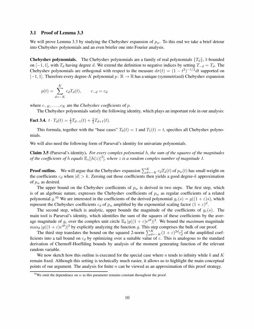
3.1 Proof of Lemma 3.3
We will prove Lemma 3.3 by studying the Chebyshev expansion of pw. To this end we take a brief detour
into Chebyshev polynomials and an even briefer one into Fourier analysis.
Chebyshev polynomials. The Chebyshev polynomials are a family of real polynomials Td, 1-bounded
on [−1, 1], with Td having degree d. We extend the definition to negative indices by setting T−d = Td. The
Chebyshev polynomials are orthogonal with respect to the measure dσ(t) = (1 − t2)−1/2dt supported on
[−1, 1]. Therefore every degree-K polynomial p : R → R has a unique (symmetrized) Chebyshev expansion
p(t) =
K∑
d=−K
cdTd(t), c−d = cd
where c−K , . . . , cK are the Chebyshev coefficients of p.
The Chebyshev polynomials satisfy the following identity, which plays an important role in our analysis:
Fact 3.4. t · Td(t) = 12Td−1(t) +
12Td+1(t).
This formula, together with the “base cases” T0(t) = 1 and T1(t) = t, specifies all Chebyshev polyno-
mials.
We will also need the following form of Parseval’s identity for univariate polynomials.
Claim 3.5 (Parseval’s identity). For every complex polynomial h, the sum of the squares of the magnitudes
of the coefficients of h equals Ez[|h(z)|2], where z is a random complex number of magnitude 1.
Proof outline. We will argue that the Chebyshev expansion∑K
d=−K cdTd(t) of pw(t) has small weight on
the coefficients cd when |d| > k. Zeroing out those coefficients then yields a good degree-k approximation
of pw as desired.
The upper bound on the Chebyshev coefficients of pw is derived in two steps. The first step, which
is of an algebraic nature, expresses the Chebyshev coefficients of pw as regular coefficients of a related
polynomial g.10 We are interested in the coefficients of the derived polynomial gε(s) = g((1 + ε)s), which
represent the Chebyshev coefficients cd of pw amplified by the exponential scaling factor (1 + ε)d.
The second step, which is analytic, upper bounds the magnitude of the coefficients of gε(s). The
main tool is Parseval’s identity, which identifies the sum of the squares of these coefficients by the aver-
age magnitude of gε over the complex unit circle Eθ |g((1 + ε)eiθ)|2. We bound the maximum magnitude
maxθ |g((1 + ε)eiθ)|2 by explicitly analyzing the function g. This step comprises the bulk of our proof.
The third step translates the bound on the squared 2-norm∑K
d=−K(1 + ε)2dc2d of the amplified coef-
ficients into a tail bound on cd by optimizing over a suitable value of ε. This is analogous to the standard
derivation of Chernoff-Hoeffding bounds by analysis of the moment generating function of the relevant
random variable.
We now sketch how this outline is executed for the special case where n tends to infinity while k and Kremain fixed. Although this setting is technically much easier, it allows us to highlight the main conceptual
points of our argument. The analysis for finite n can be viewed as an approximation of this proof strategy.
10We omit the dependence on w as this parameter remains constant throughout the proof.
10
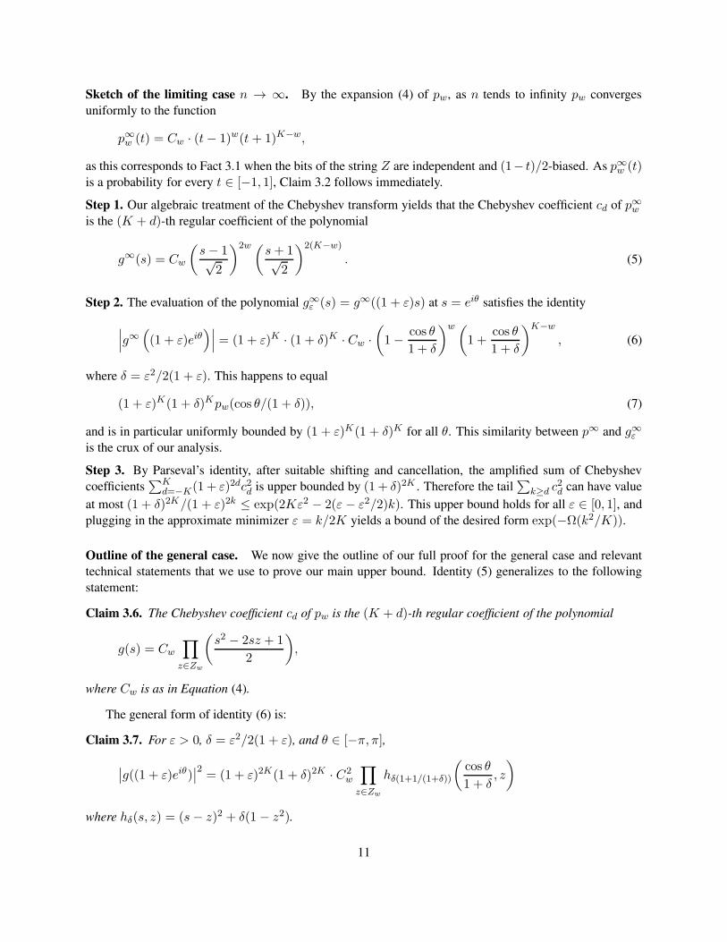
Sketch of the limiting case n → ∞. By the expansion (4) of pw, as n tends to infinity pw converges
uniformly to the function
p∞w (t) = Cw · (t− 1)w(t+ 1)K−w,
as this corresponds to Fact 3.1 when the bits of the string Z are independent and (1− t)/2-biased. As p∞w (t)is a probability for every t ∈ [−1, 1], Claim 3.2 follows immediately.
Step 1. Our algebraic treatment of the Chebyshev transform yields that the Chebyshev coefficient cd of p∞wis the (K + d)-th regular coefficient of the polynomial
g∞(s) = Cw
(s− 1√
2
)2w (s+ 1√2
)2(K−w)
. (5)
Step 2. The evaluation of the polynomial g∞ε (s) = g∞((1 + ε)s) at s = eiθ satisfies the identity
∣∣∣g∞((1 + ε)eiθ
)∣∣∣ = (1 + ε)K · (1 + δ)K · Cw ·(1− cos θ
1 + δ
)w (1 +
cos θ
1 + δ
)K−w
, (6)
where δ = ε2/2(1 + ε). This happens to equal
(1 + ε)K(1 + δ)Kpw(cos θ/(1 + δ)), (7)
and is in particular uniformly bounded by (1 + ε)K(1 + δ)K for all θ. This similarity between p∞ and g∞εis the crux of our analysis.
Step 3. By Parseval’s identity, after suitable shifting and cancellation, the amplified sum of Chebyshev
coefficients∑K
d=−K(1 + ε)2dc2d is upper bounded by (1 + δ)2K . Therefore the tail∑
k≥d c2d can have value
at most (1 + δ)2K/(1 + ε)2k ≤ exp(2Kε2 − 2(ε − ε2/2)k). This upper bound holds for all ε ∈ [0, 1], and
plugging in the approximate minimizer ε = k/2K yields a bound of the desired form exp(−Ω(k2/K)).
Outline of the general case. We now give the outline of our full proof for the general case and relevant
technical statements that we use to prove our main upper bound. Identity (5) generalizes to the following
statement:
Claim 3.6. The Chebyshev coefficient cd of pw is the (K + d)-th regular coefficient of the polynomial
g(s) = Cw
∏
z∈Zw
(s2 − 2sz + 1
2
),
where Cw is as in Equation (4).
The general form of identity (6) is:
Claim 3.7. For ε > 0, δ = ε2/2(1 + ε), and θ ∈ [−π, π],∣∣g((1 + ε)eiθ)
∣∣2 = (1 + ε)2K(1 + δ)2K · C2w
∏
z∈Zw
hδ(1+1/(1+δ))
(cos θ
1 + δ, z
)
where hδ(s, z) = (s− z)2 + δ(1 − z2).
11

Owing to the second term in hδ, there is no identity analogous to (7) when n is finite and pw has
zeros inside (−1, 1). Nevertheless,∏
z∈Zwhδ(s, z) can be uniformly bounded either by a sufficiently small
multiple of pw(s)2, or a fixed quantity that is constant in the parameter range of interest.
Claim 3.8. Assume n ≥ 64K and w ≤ K/2. Then
C2w ·
∏
z∈Zw
hδ(s, z) ≤e65δK · pw(s)2 if |s| ≤ 1− w/16K
e65δK if 1− w/16K ≤ |s| ≤ 1.
We now prove Lemma 3.3. Claim 3.6 is proved in Section 3.2. Claim 3.7 is proved in Section 3.3.
Claims 3.2 and 3.8 are proved in Section 3.4 as the proofs share the same structure.
Fact 3.9. pw(t) = pK−w(1− t).
Proof. By Fact 3.1, both sides are degree-K polynomials that agree on n + 1 > K points so they are
identical.
Proof of Lemma 3.3. By Fact 3.9 we may and will assume that w ≤ K/2. Let pw =∑K
d=−K cdTd. The
approximating polynomial qw is∑
|d|<k cdTd. It remains to prove a tail upper bound on the Chebyshev
coefficients. By Claim 3.6, the (K+d)-th coefficient of g(s) is cd. Therefore the polynomial gε(s) = g((1+ε)s) has coefficients (1 + ε)K+dcd as d ranges from −K to K . We apply Parseval’s identity (Claim 3.5) to
gε.
It follows that
K∑
d=−K
(1 + ε)2(K+d)c2d = Eθ |g((1 + ε)eiθ)|2
≤ maxθ∈[−π,π]
|g((1 + ε)eiθ)|2
= maxs∈[−1,1]
(1 + ε)2K(1 + δ)2K · C2w
∏
z∈Zw
hδ(1+1/(1+δ))(s/(1 + δ), z),
by Claim 3.7. Since 0 ≤ δ = ε2/2(1+ ε) ≤ 1/2, for simplicity we may replace hδ(1+1/(1+δ))(s/(1+ δ), z)by h2δ(s, z) in the above inequality. This gives the following approximation bound for α = maxt∈[−1,1] |pw(t)−qw(t)|:
α = maxt∈[−1,1]
∣∣∣∑
|d|≥kcdTd(t)
∣∣∣
≤∑
|d|≥k|cd| max
t∈[−1,1]|Td(t)|
≤ 2∑
d≥k
|cd| (by symmetry and boundedness of Td)
≤ 2√K ·
√∑d≥k
c2d (by Cauchy-Schwarz)
≤ 2√K ·
√(1 + ε)−2(K+k)
∑d≥k
(1 + ε)2(K+d)c2d
≤ 2√K
√(1 + ε)−2k · (1 + δ)2K · max
s∈[−1,1]C2w
∏
z∈Zw
h2δ(s, z).
12
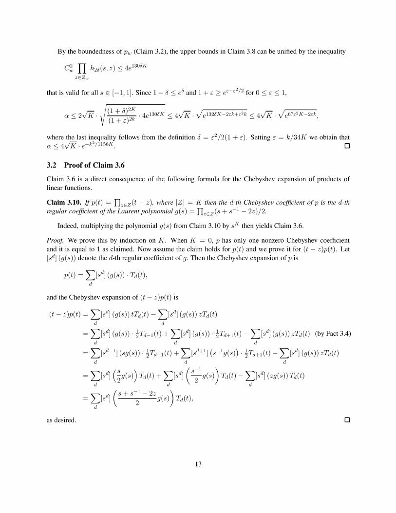
By the boundedness of pw (Claim 3.2), the upper bounds in Claim 3.8 can be unified by the inequality
C2w
∏
z∈Zw
h2δ(s, z) ≤ 4e130δK
that is valid for all s ∈ [−1, 1]. Since 1 + δ ≤ eδ and 1 + ε ≥ eε−ε2/2 for 0 ≤ ε ≤ 1,
α ≤ 2√K ·
√(1 + δ)2K
(1 + ε)2k· 4e130δK ≤ 4
√K ·
√e132δK−2εk+ε2k ≤ 4
√K ·
√e67ε2K−2εk,
where the last inequality follows from the definition δ = ε2/2(1 + ε). Setting ε = k/34K we obtain that
α ≤ 4√K · e−k2/1156K .
3.2 Proof of Claim 3.6
Claim 3.6 is a direct consequence of the following formula for the Chebyshev expansion of products of
linear functions.
Claim 3.10. If p(t) =∏
z∈Z(t − z), where |Z| = K then the d-th Chebyshev coefficient of p is the d-th
regular coefficient of the Laurent polynomial g(s) =∏
z∈Z(s+ s−1 − 2z)/2.
Indeed, multiplying the polynomial g(s) from Claim 3.10 by sK then yields Claim 3.6.
Proof. We prove this by induction on K . When K = 0, p has only one nonzero Chebyshev coefficient
and it is equal to 1 as claimed. Now assume the claim holds for p(t) and we prove it for (t − z)p(t). Let
[sd] (g(s)) denote the d-th regular coefficient of g. Then the Chebyshev expansion of p is
p(t) =∑
d
[sd] (g(s)) · Td(t),
and the Chebyshev expansion of (t− z)p(t) is
(t− z)p(t) =∑
d
[sd] (g(s)) tTd(t)−∑
d
[sd] (g(s)) zTd(t)
=∑
d
[sd] (g(s)) · 12Td−1(t) +
∑
d
[sd] (g(s)) · 12Td+1(t)−
∑
d
[sd] (g(s)) zTd(t) (by Fact 3.4)
=∑
d
[sd−1] (sg(s)) · 12Td−1(t) +
∑
d
[sd+1](s−1g(s)
)· 12Td+1(t)−
∑
d
[sd] (g(s)) zTd(t)
=∑
d
[sd](s2g(s)
)Td(t) +
∑
d
[sd]
(s−1
2g(s)
)Td(t)−
∑
d
[sd] (zg(s))Td(t)
=∑
d
[sd]
(s+ s−1 − 2z
2g(s)
)Td(t),
as desired.
13
3.3 Proof of Claim 3.7
Proof. By definition of Zw, we have that z ∈ [−1, 1] and thus may set z = cosφ. We also write s =(1 + ε)eiθ = (1 + ε) cos θ + i(1 + ε) sin θ, from which it follows that:
s2 − 2sz + 1 = (s− z +√z2 − 1)(s − z −
√z2 − 1) = (s− cosφ+ i sinφ)(s − cosφ− i sinφ)
= (s− eiφ)(s − e−iφ) = ((1 + ε)eiθ − eiφ)((1 + ε)eiθ − e−iφ)
=((1 + ε)ei(θ+φ) − 1
)((1 + ε)ei(θ−φ) − 1
).
Recalling that δ = ε2
2(1+ε) , we have that for any γ,
|(1 + ε)eiγ − 1|2 = (−1 + (1 + ε) cos γ)2 + ((1 + ε) sin γ)2
= 1− 2(1 + ε) cos γ + (1 + ε)2
= 2(1 + ε)(1 − cos γ + δ),
from which it follows that
|s2 − 2sz + 1|2 =∣∣∣(1 + ε)ei(θ+φ) − 1
∣∣∣2 ∣∣∣(1 + ε)ei(θ−φ) − 1
∣∣∣2
= 4(1 + ε)2(1− cos(θ + φ) + δ) · (1− cos(θ − φ) + δ)
= 4(1 + ε)2(1 + δ)2(1− cos(θ + φ)
1 + δ
)(1− cos(θ − φ)
1 + δ
)
= 4(1 + ε)2(1 + δ)2
((1− cos θ cosφ
1 + δ
)2
−(sin θ sinφ
1 + δ
)2)
= 4(1 + ε)2(1 + δ)2
((1− z cos θ
1 + δ
)2
−((1− z2) sin2 θ
(1 + δ)2
))
= 4(1 + ε)2((1 + δ − z cos θ)2 − (1− z2) sin2 θ
)
= 4(1 + ε)2((1 + δ)2 − 2(1 + δ)z cos θ − 1 + z2 + cos2 θ
)
= 4(1 + ε)2((cos θ − (1 + δ)z)2 + (1− z2)(2δ + δ2)
).
Note that the fourth equality uses the sum and difference formulas for sine and cosine.
We then have
∣∣∣∣s2 − 2sz + 1
2
∣∣∣∣2
= (1 + ε)2((cos θ − (1 + δ)z)2 + (1− z2)(2δ + δ2)
)
= (1 + ε)2(1 + δ)2
((cos θ
1 + δ− z
)2
+(1− z2)(2δ + δ2)
1 + δ
).
The claim then follows by multiplicativity of the norm.
14
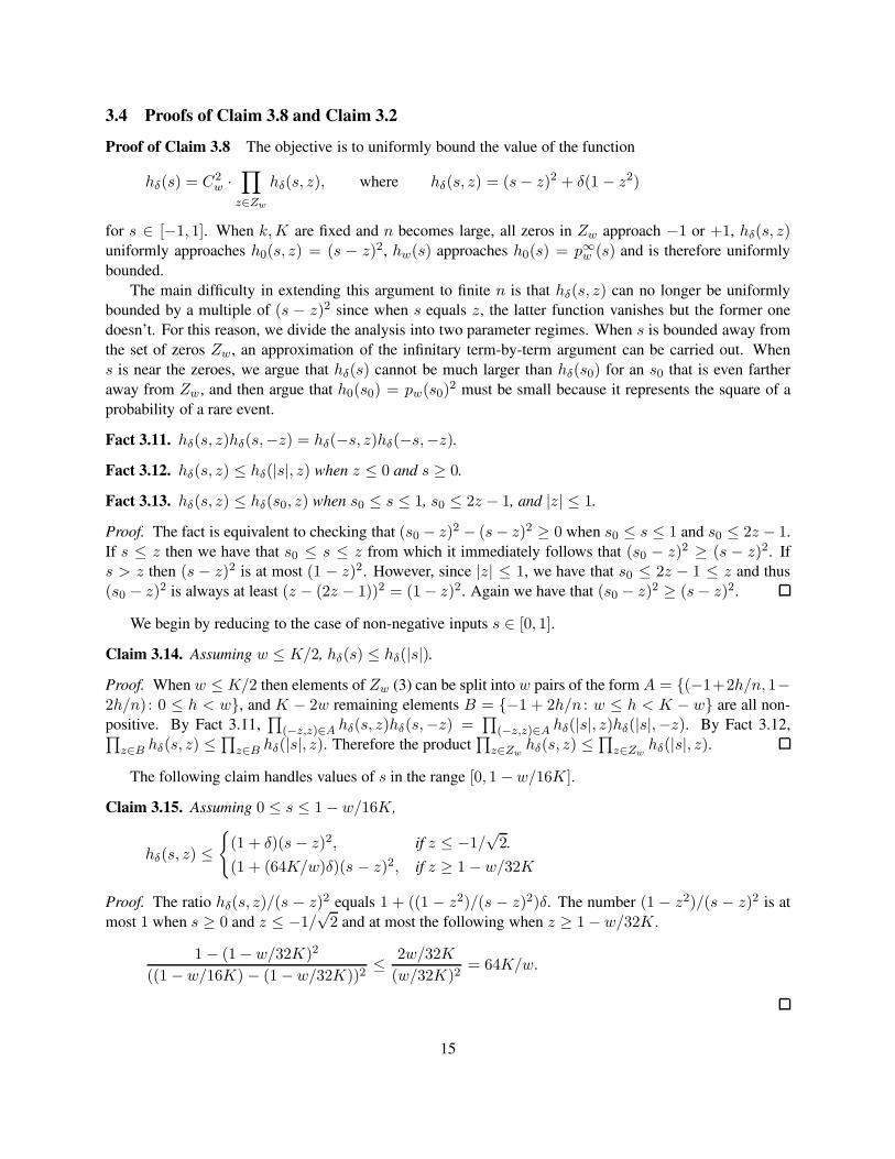
3.4 Proofs of Claim 3.8 and Claim 3.2
Proof of Claim 3.8 The objective is to uniformly bound the value of the function
hδ(s) = C2w ·
∏
z∈Zw
hδ(s, z), where hδ(s, z) = (s− z)2 + δ(1 − z2)
for s ∈ [−1, 1]. When k,K are fixed and n becomes large, all zeros in Zw approach −1 or +1, hδ(s, z)uniformly approaches h0(s, z) = (s − z)2, hw(s) approaches h0(s) = p∞w (s) and is therefore uniformly
bounded.
The main difficulty in extending this argument to finite n is that hδ(s, z) can no longer be uniformly
bounded by a multiple of (s − z)2 since when s equals z, the latter function vanishes but the former one
doesn’t. For this reason, we divide the analysis into two parameter regimes. When s is bounded away from
the set of zeros Zw, an approximation of the infinitary term-by-term argument can be carried out. When
s is near the zeroes, we argue that hδ(s) cannot be much larger than hδ(s0) for an s0 that is even farther
away from Zw, and then argue that h0(s0) = pw(s0)2 must be small because it represents the square of a
probability of a rare event.
Fact 3.11. hδ(s, z)hδ(s,−z) = hδ(−s, z)hδ(−s,−z).
Fact 3.12. hδ(s, z) ≤ hδ(|s|, z) when z ≤ 0 and s ≥ 0.
Fact 3.13. hδ(s, z) ≤ hδ(s0, z) when s0 ≤ s ≤ 1, s0 ≤ 2z − 1, and |z| ≤ 1.
Proof. The fact is equivalent to checking that (s0 − z)2 − (s− z)2 ≥ 0 when s0 ≤ s ≤ 1 and s0 ≤ 2z − 1.
If s ≤ z then we have that s0 ≤ s ≤ z from which it immediately follows that (s0 − z)2 ≥ (s − z)2. If
s > z then (s − z)2 is at most (1 − z)2. However, since |z| ≤ 1, we have that s0 ≤ 2z − 1 ≤ z and thus
(s0 − z)2 is always at least (z − (2z − 1))2 = (1 − z)2. Again we have that (s0 − z)2 ≥ (s− z)2.
We begin by reducing to the case of non-negative inputs s ∈ [0, 1].
Claim 3.14. Assuming w ≤ K/2, hδ(s) ≤ hδ(|s|).
Proof. When w ≤ K/2 then elements of Zw (3) can be split into w pairs of the formA = (−1+2h/n, 1−2h/n) : 0 ≤ h < w, and K − 2w remaining elements B = −1 + 2h/n : w ≤ h < K − w are all non-
positive. By Fact 3.11,∏
(−z,z)∈A hδ(s, z)hδ(s,−z) =∏
(−z,z)∈A hδ(|s|, z)hδ(|s|,−z). By Fact 3.12,∏z∈B hδ(s, z) ≤
∏z∈B hδ(|s|, z). Therefore the product
∏z∈Zw
hδ(s, z) ≤∏
z∈Zwhδ(|s|, z).
The following claim handles values of s in the range [0, 1 −w/16K].
Claim 3.15. Assuming 0 ≤ s ≤ 1− w/16K ,
hδ(s, z) ≤(1 + δ)(s − z)2, if z ≤ −1/
√2.
(1 + (64K/w)δ)(s − z)2, if z ≥ 1− w/32K
Proof. The ratio hδ(s, z)/(s − z)2 equals 1 + ((1 − z2)/(s − z)2)δ. The number (1 − z2)/(s − z)2 is at
most 1 when s ≥ 0 and z ≤ −1/√2 and at most the following when z ≥ 1− w/32K .
1− (1− w/32K)2
((1 − w/16K) − (1−w/32K))2≤ 2w/32K
(w/32K)2= 64K/w.
15
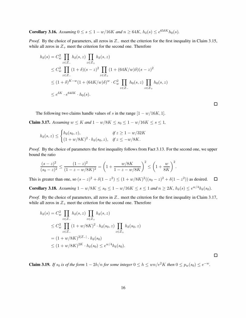
Corollary 3.16. Assuming 0 ≤ s ≤ 1−w/16K and n ≥ 64K , hδ(s) ≤ e65δKh0(s).
Proof. By the choice of parameters, all zeros in Z− meet the criterion for the first inequality in Claim 3.15,
while all zeros in Z+ meet the criterion for the second one. Therefore
hδ(s) = C2w
∏
z∈Z−
hδ(s, z)∏
z∈Z+
hδ(s, z)
≤ C2w
∏
z∈Z−
(1 + δ)(s − z)2∏
z∈Z+
(1 + (64K/w)δ)(s − z)2
≤ (1 + δ)K−w(1 + (64K/w)δ)w · C2w
∏
z∈Z−
h0(s, z)∏
z∈Z+
h0(s, z)
≤ eδK · e64δK · h0(s).
The following two claims handle values of s in the range [1− w/16K, 1].
Claim 3.17. Assuming w ≤ K and 1− w/8K ≤ s0 ≤ 1− w/16K ≤ s ≤ 1,
hδ(s, z) ≤hδ(s0, z), if z ≥ 1− w/32K
(1 + w/8K)2 · hδ(s0, z), if z ≤ −w/8K.
Proof. By the choice of parameters the first inequality follows from Fact 3.13. For the second one, we upper
bound the ratio
(s− z)2
(s0 − z)2≤ (1− z)2
(1− z − w/8K)2=
(1 +
w/8K
1− z − w/8K
)2
≤(1 +
w
8K
)2
.
This is greater than one, so (s − z)2 + δ(1− z2) ≤ (1 + w/8K)2((s0 − z)2 + δ(1− z2)) as desired.
Corollary 3.18. Assuming 1− w/8K ≤ s0 ≤ 1− w/16K ≤ s ≤ 1 and n ≥ 2K , hδ(s) ≤ ew/4hδ(s0).
Proof. By the choice of parameters, all zeros in Z− meet the criterion for the first inequality in Claim 3.17,
while all zeros in Z+ meet the criterion for the second one. Therefore
hδ(s) = C2w
∏
z∈Z−
hδ(s, z)∏
z∈Z+
hδ(s, z)
≤ C2w
∏
z∈Z−
(1 + w/8K)2 · hδ(s0, z)∏
z∈Z+
hδ(s0, z)
= (1 + w/8K)2|Z−| · hδ(s0)≤ (1 + w/8K)2K · hδ(s0) ≤ ew/4hδ(s0).
Claim 3.19. If s0 is of the form 1− 2h/n for some integer 0 ≤ h ≤ wn/e2K then 0 ≤ pw(s0) ≤ e−w.
16

Proof. By Fact 3.1, pw(s0) is the probability that a random string of Hamming weight h and length n has
exactly w ones in its first K positions. The probability that it has at least w ones in its first K positions is at
most(K
w
)· hn· h− 1
n− 1· · · h− w + 1
n− w + 1≤(eK
w
)w(hn
)w
≤ e−w.
Proof of Claim 3.8. By Claim 3.14 we may assume s ∈ [0, 1]. When 0 ≤ s ≤ 1−w/16K the result follows
from Corollary 3.16. When 1−w/16K ≤ |s| ≤ 1, by the assumption n ≥ 64K there must exist a value s0between 1− w/8K and 1− w/16K that is of the form 1− 2h/n. In particular h ≤ wn/e2K . Then
hδ(s) ≤ ew/4hδ(s0) ≤ ew/4e65δKpw(s0)2 ≤ e65δK−7w/4,
where the inequalities follow from Corollary 3.18, Corollary 3.16, and Claim 3.19, respectively.
Proof of Claim 3.2 This proof has a similar structure to that of Claim 3.8. By symmetry we can again
restrict attention to inputs t ∈ [0, 1]. When t ≤ 1−2w/n then |pw(t)| is not much larger than |pw(t′)| where
t′ is the largest number of the form 1 − 2h/n not exceeding t for integer h. Otherwise the value |pw(t)| is
not much larger than |pw(s0)|, for some s0 ∈ [1−w/8K, 1−w/16K] of the form 1− 2h/n for an integer
h. In turn, pw(s0) is the probability of a rare event, so we conclude that |pw(t)| is small.
Claim 3.20. If −2/n ≤ t′ ≤ t ≤ 1− 2w/n then
|t− z| ≤|t′ − z|, if z ≥ 1− 2w/n,
(1 + 2(t− t′))|t′ − z|, if z ≤ −1/2− 2/n.
Proof. The first part follows because the expressions under the absolute value are nonnegative. For the
second part, we bound the ratio
t− z
t′ − z= 1 +
t− t′
t′ − z≤ 1 + 2(t− t′)
as desired.
Corollary 3.21. Assuming n ≥ 64K and −2/n ≤ t′ ≤ t ≤ 1− 2w/n, |pw(t)| ≤ (1 + 2(t− t′))K |pw(t′)|.
Proof. By the choice of parameters, all zeros in Z+ meet the criterion for the first inequality in Claim 3.20,
while all zeros in Z− meet the criterion for the second one. Therefore
|pw(t)| = Cw
∏
z∈Z−
|t− z|∏
z∈Z+
|t− z|
≤ Cw
∏
z∈Z−
(1 + 2(t− t′))∣∣t′ − z
∣∣ ∏
z∈Z+
∣∣t′ − z∣∣
= (1 + 2(t− t′))|Z−| ·∣∣pw(t′)
∣∣
≤ (1 + 2(t− t′))K ·∣∣pw(t′)
∣∣.
17
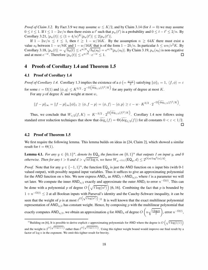
Proof of Claim 3.2. By Fact 3.9 we may assume w ≤ K/2, and by Claim 3.14 (for δ = 0) we may assume
0 ≤ t ≤ 1. If t ≤ 1− 2w/n then there exists a t′ such that pw(t′) is a probability and 0 ≤ t− t′ ≤ 2/n. By
Corollary 3.21, |pw(t)| ≤ (1 + 4/n)K |pw(t′)| ≤ 2|pw(t′)|.If 1 − 2w/n ≤ t ≤ 1, then t ≥ 1 − w/16K . By the assumption n ≥ 64K there must exist a
value s0 between 1− w/8K and 1−w/16K that is of the form 1− 2h/n. In particular h ≤ wn/e2K . By
Corollary 3.18, |pw(t)| =√h0(t) ≤ ew/8
√h0(s0) = ew/8|pw(s0)|. By Claim 3.19, pw(s0) is non-negative
and at most e−w. Therefore |pw(t)| ≤ ew/8 · e−w ≤ 1.
4 Proofs of Corollary 1.4 and Theorem 1.5
4.1 Proof of Corollary 1.4
Proof of Corollary 1.4. Corollary 1.3 implies the existence of a φ(= µ−ν
2
)satisfying ‖φ‖1 = 1, 〈f, φ〉 = ε
for some ε = Ω(1) and 〈φ, q〉 ≤ K3/2 · 2−Ω(deg1/3(f)
2/K)
for any parity of degree at most K .
For any p of degree K and weight at most w,
‖f − p‖∞ = ‖f − p‖∞‖φ‖1 ≥ 〈φ, f − p〉 = 〈φ, f〉 − 〈φ, p〉 ≥ ε− w ·K3/2 · 2−Ω(deg1/3(f)
2/K)
.
Thus, we conclude that Wε/2(f,K) = K−3/2 · 2Ω(deg1/3(f)
2/K)
. Corollary 1.4 now follows using
standard error reduction techniques that show that degε(f) = Θ(deg1/3(f)) for all constants 0 < ε < 1/2.
4.2 Proof of Theorem 1.5
We first require the following lemma. This lemma builds on ideas in [24, Claim 2], which showed a similar
result for t = Θ(1).
Lemma 4.1. For any y ∈ 0, 1n, denote by EQy the function on 0, 1n that outputs 1 on input y, and 0
otherwise. Then for any t > 0 and d >√nt log n, we have Wn−O(t)(EQy, d) ≤ 2O(nt log2(n)/d).
Proof. Note that for any y ∈ −1, 1n, the function EQy is just the AND function on n input bits (with 0-1
valued output), with possibly negated input variables. Thus it suffices to give an approximating polynomial
for the AND function on n bits. We now express ANDn as ANDℓ ANDn/ℓ, where ℓ is a parameter we will
set later. We compute the inner ANDn/ℓ exactly and approximate the outer ANDℓ to error n−Ω(t). This can
be done with a polynomial p of degree O(√
ℓ log(nt))
[6, 16]. Combining the fact that p is bounded by
1 + n−Ω(t) ≤ 2 at all Boolean inputs with Parseval’s identity and the Cauchy-Schwarz inequality, it can be
seen that the weight of p is at most ℓO(√
ℓ log(nt))
.11 It is well known that the exact multilinear polynomial
representation of ANDn/ℓ has constant weight. Hence, by composing p with the multilinear polynomial that
exactly computes ANDn/ℓ, we obtain an approximation q for ANDn of degree O
(n√
t lognℓ
), error n−Ω(t),
11Building on [6], It is possible to derive explicit ε-approximating polynomials for AND where the degree is O(√
ℓ log(1/ε))
and the weight is 2O(√
ℓ log(1/ε)
rather than ℓO(√
ℓ log(1/ε))
. Using this tighter weight bound would improve our final result by a
factor of log n in the exponent. We omit this tighter result for brevity.
18

and weight 2O(√
ℓt log3 n)
. We now fix the value of ℓ to ℓ := n2t lognd2
< n, thereby ensuring that the degree
of q is at most d. With this setting of ℓ, the weight of q is at most 2O(nt log2(n)/d), proving the lemma.
Proof of Theorem 1.5. Let f : 0, 1n → 0, 1 be any symmetric function, corresponding to the univariate
predicate Df : 0 ∪ [n] → 0, 1n. For the purpose of this proof, let us denote by kf the smallest i for
which f is constant on inputs of Hamming weight in the interval [i+1, n−i−1]. Without loss of generality,
f(x) = 0 for strings of x Hamming weight between kf +1 and n− kf − 1. The case where f = 1 on input
strings of Hamming weight between kf +1 and n− kf − 1 can be proved using a similar argument. Define
supp(f) := x ∈ 0, 1n : f(x) = 1. Note that |supp(f)| ≤ 2 · nkf .
Observe that f(x) =∑
y∈supp(f) EQy(x). Lemma 4.1 implies, for each y ∈ supp(f), the existence
of polynomials py of degree K and weight 2O(nkf log2(n)/K), which approximate EQy to error 16 · n−kf .
Define a polynomial p : 0, 1n → R by p(x) =∑
y∈supp(f) py(x). Clearly p has degree K , weight at
most nO(kf ) · 2O(nkf log2(n)/K) = 2O(nkf/K), and error at most |supp(f)| · n−kf /6 ≤ 1/3, where the upper
bounds on the weight and error follow from the triangle inequality.
The theorem now follows standard error reduction techniques and Paturi’s theorem [22], which states
that for symmetric functions, deg(f) = Θ(√
n · kf).
Remark 4.2. The upper bound obtained in Theorem 1.5 is more general than as stated, and the only prop-
erty of symmetric functions it exploits is that symmetric functions of low approximate degree are highly
biased. More specifically, the proof of Theorem 1.5 shows that any function f : 0, 1n → 0, 1 with
min|f−1(0)|, |f−1(1)| ≤ nt satisfies Wε(f,K) ≤ 2O(nt/K) for any K ≥√nt log n.
5 Proof of Theorem 1.6
Proof outline. As we explain in more detail in the proof itself, it is sufficient to establish the theorem for
fixed k and K and infinitely many n because the statement is downward reducible in n.
Using the Chebyshev approximation formulas from Section 3 we derive explicit lower bounds on the
large Chebyshev coefficients on the polynomial p0 representing the distinguishing advantage of the AND
function on K inputs. Owing to orthogonality and boundedness of the Chebyshev polynomials, this is
a lower bound on the approximate degree of ANDK . By strong duality as given in the following Claim
(see [4]) we obtain Theorem 1.6.
Claim 5.1. If degε/2(Fn) ≥ k then there exists a pair of perfectly k-wise indistinguishable distributions µ,
ν over 0, 1n such that EX∼µ[Fn(X)]− EY∼ν [Fn(Y )] ≥ ε.
Recall that the Chebyshev polynomials are orthogonal under the measure dσ(t) = (1 − t2)−1/2dtsupported on [−1, 1]. We will need the following identity for their average square magnitude under this
measure:
Et∼σ[Td(t)2] = 1/2 when d > 0. (8)
Proof of Theorem 1.6. By symmetry of the distinguishers, µ and ν can be assumed symmetric. Let Fn
denote the function on 0, 1n that outputs ANDK
(x|1,...,K
), i.e., Fn outputs the AND of the first K < n
bits of the input. We prove the theorem for Gn(x1, . . . , xn) = NOR(x|1,...,K). By the symmetry of 0 and
1 inputs the theorem also holds for Fn.
19
First, we claim that the statement of Theorem 1.6 is stronger as n becomes larger, so it is sufficient
to prove it in the limiting case when n approaches infinity and k,K are fixed. Suppose that µ and νare distributions over n bit strings that are k-wise indistinguishable yet are ε-reconstructable by Gn. We
must show that there are distributions µ′ and ν ′ over 0, 1n−1 are k-wise indistinguishable yet are ε-reconstructable by Gn−1. But this holds for µ′ (respectively ν ′) that generate a random sample from µ(respectively, ν) and then throw away the last bit.
If the statement was false then by Claim 5.1 there would exist degree-k polynomials Gn that approximate
Gn pointwise on 0, 1n to within error ε =
√2−4K+1
∑d>K
( 2KK+d
)2for almost all n. Applying the
construction from the proof of Fact 3.1 to Gn, there exist univariate degree-k polynomials pn0 approximating
pn0 on the set of points Wn = −1 + 2h/n : 0 ≤ h ≤ n to within error ε. We emphasize the dependence
on n as it will play a role in the proof.
By Formula (3) the polynomial pn0 has the form
pn0 (t) = Cn0
∏
z∈Zn0
(t− z),
where Zn0 = −1 + 2h/n : 0 ≤ h < K (the set Z+ is empty). The value p0n(1) is the probability that Gn
accepts the all-zero string, so it must equal one. The constant Cn0 must therefore equal
∏z∈Zn
0(1 − z)−1.
As n tends to infinity, the set Z0 converges to a single zero at −1 of multiplicity K , so the sequence pn0converges uniformly to the polynomial
p∞0 (t) = 2−K(t+ 1)K .
By the triangle inequality, for every δ > 0 and all sufficiently large n, pn0 is within ε + δ of p∞0 on the set
Wn. A degree-k polynomial is determined by its values on Wk+1 and the set of degree-k polynomials that
are within ε+ δ of p∞0 on Wk+1 is compact. Therefore the sequence of approximating polynomials pn0 must
contain a subsequence (for values of n that are multiples of k + 1) that converges (uniformly) to a limiting
degree-k polynomial p∞0 . Since pn0 is within ε + δ of pn0 on Wn for infinitely many n, p∞0 must be within
ε+2δ of p∞0 on Wn for infinitely many n. The union of these sets Wn is dense in [−1, 1], and by continuity
p∞0 can be ε+ δ-approximated by the degree-k polynomial p∞0 everywhere on [−1, 1]. As δ was arbitrary it
follows that the ε-approximate degree of p∞0 can be at most k.
All that remains to prove that this is not true, i.e., to show a lower bound of k on the ε-approximate
degree of p∞0 . This lower bound is known (see, e.g., [14]); we provide the details now for completeness. Let
q be any degree-k polynomial. By Claim 3.6 the d-th Chebyshev coefficient of p∞0 equals the (K + d)-thregular coefficient of g∞(s) = 2−2K(s+1)2K , which has value 2−2K
( 2KK+d
). Since q has degree at most k,
the d-th Chebyshev coefficient cd of p∞0 − q must also equal 2−2K( 2KK+d
)whenever |d| > k. By symmetry
of the Chebyshev coefficients, orthogonality of the Chebyshev polynomials, and Equation (8),
Et∼σ[(p∞0 (t)− q(t))2] = c20 +
∑d>0
(2cd)2Et∼σ [Td(t)
2] ≥∑
d>k2 ·(2−2K
(2K
K + d
))2
= ε2.
It follows that the approximation error |p∞0 (t)− q(t)| must exceed ε for some t ∈ [−1, 1], contradicting the
initial assumption.
6 Robustness of Symmetric Secret Sharing Against Consolidation
Consider a secret sharing scheme with tn parties, divided in n blocks of size t, that is perfectly secure
against size-k coalitions. If all parties in each block come together and consolidate their information even
20
into a single bit, the number of blocks against which the scheme remains secure drops to k/t. In general this
is the best possible, with linear schemes providing tight examples.
The following corollary shows that if the distribution over shares is symmetric then much better security
against this type of attack can be obtained.
Corollary 6.1. Let f1, . . . , fn : 0, 1t → 0, 1. Assume X,Y are k-wise indistinguishable symmetri-
cally distributed random variables over tn-bit strings. Write X = X1 . . . Xn, Y = Y1 . . . Yn, where
all blocks Xi, Yi have size t. For every K , the n-bit random variables X ′ = f1(X1) . . . fn(Xn) and
Y ′ = f1(Y1) . . . fn(Yn) are O((tK)3/2nKe−k2/1156tK)-close to being perfectly K-wise indistinguishable,
assuming K ≤ n/64.
The resulting scheme can be viewed as perfectly secure secret sharing with a potentially faulty dealer:
With probability 1 − p, the dealer samples perfectly K-wise indistinguishable shares X ′ or Y ′, and with
probability p = O((tK)3/2nKe−k2/1156tK ) she leaks arbitrary information about the secret.
For example, ifX,Y are visual shares sampled from the dual polynomial (1) then they are k = Ω(√tn)-
wise indistinguishable, assuming constant reconstruction error. Corollary 6.1 then says that the induced
block-shares X ′, Y ′ are Ω(√n/ log n)-wise indistinguishable except with probability exp−Ω(
√n log n).
If, in addition, f1 = · · · = fn = ANDt then X ′, Y ′ are themselves shares of a visual secret sharing
scheme that is secure against Ω(√n/ log n)-size coalitions. Therefore symmetric visual secret sharing
schemes are downward self-reducible at a small loss in security and dealer error in the following sense: A
scheme for n parties can be derived from one for tn parties by dividing the parties into blocks and ANDing
the shares in each block.
Proof of Corollary 6.1. By Theorem 1.2, X and Y are (tK,O((tK)3/2) · e−k2/1156tK)-wise indistinguish-
able. Since any size-K distinguisher against (X ′, Y ′) induces a size-tK distinguisher against (X,Y ), the
former are (K, δ = O((tK)3/2) · e−k2/1156tK)-wise indistinguishable. By Theorem D.1 of [4], any pair of
(K, δ)-wise indistinguishable distributions over n bits is 2δnK -close to a pair of perfectly indistinguishable
ones.
7 Acknowledgements
We thank Mark Bun for telling us about the work of Sachdeva and Vishnoi [23], and Mert Saglam, Pritish
Kamath, Robin Kothari, and Prashant Nalini Vasudevan for helpful comments on a previous version of the
manuscript. We are also grateful to Xuangui Huang and Emanuele Viola for sharing the manuscript [15].
Andrej Bogdanov’s work was supported by RGC GRF CUHK14207618. Justin Thaler and Nikhil Mande
were supported by NSF Grant CCF-1845125.
References
[1] Andris Ambainis. Quantum search with variable times. Theory Comput. Syst., 47(3):786–807, 2010.
[2] Shalev Ben-David, Adam Bouland, Ankit Garg, and Robin Kothari. Classical lower bounds from
quantum upper bounds. In 59th IEEE Annual Symposium on Foundations of Computer Science, FOCS
2018, Paris, France, October 7-9, 2018, pages 339–349, 2018.
[3] Andrej Bogdanov. Approximate degree of AND via Fourier analysis. Electronic Colloquium on
Computational Complexity (ECCC), 25:197, 2018.
21
[4] Andrej Bogdanov, Yuval Ishai, Emanuele Viola, and Christopher Williamson. Bounded indistinguisha-
bility and the complexity of recovering secrets. In Advances in Cryptology - CRYPTO 2016 - 36th
Annual International Cryptology Conference, Santa Barbara, CA, USA, August 14-18, 2016, Proceed-
ings, Part III, pages 593–618, 2016.
[5] Andrej Bogdanov and Christopher Williamson. Approximate bounded indistinguishability. In 44th
International Colloquium on Automata, Languages, and Programming, ICALP 2017, July 10-14, 2017,
Warsaw, Poland, pages 53:1–53:11, 2017.
[6] Harry Buhrman, Richard Cleve, Ronald de Wolf, and Christof Zalka. Bounds for small-error and zero-
error quantum algorithms. In 40th Annual Symposium on Foundations of Computer Science, FOCS
’99, 17-18 October, 1999, New York, NY, USA, pages 358–368, 1999.
[7] Mark Bun, Robin Kothari, and Justin Thaler. The polynomial method strikes back: tight quantum
query bounds via dual polynomials. In Proceedings of the 50th Annual ACM SIGACT Symposium on
Theory of Computing, STOC 2018, Los Angeles, CA, USA, June 25-29, 2018, pages 297–310, 2018.
[8] Mark Bun and Justin Thaler. Dual lower bounds for approximate degree and markov-bernstein in-
equalities. In Automata, Languages, and Programming - 40th International Colloquium, ICALP 2013,
Riga, Latvia, July 8-12, 2013, Proceedings, Part I, pages 303–314, 2013.
[9] Mark Bun and Justin Thaler. Hardness amplification and the approximate degree of constant-depth cir-
cuits. Electronic Colloquium on Computational Complexity (ECCC), 20:151, 2013. Extended abstract
in ICALP 2015.
[10] Mark Bun and Justin Thaler. Hardness amplification and the approximate degree of constant-depth
circuits. In Automata, Languages, and Programming - 42nd International Colloquium, ICALP 2015,
Kyoto, Japan, July 6-10, 2015, Proceedings, Part I, pages 268–280, 2015.
[11] Mark Bun and Justin Thaler. A nearly optimal lower bound on the approximate degree of AC0. In
58th IEEE Annual Symposium on Foundations of Computer Science, FOCS 2017, Berkeley, CA, USA,
October 15-17, 2017, pages 1–12, 2017.
[12] Mark Bun and Justin Thaler. The large-error approximate degree of AC0. Electronic Colloquium on
Computational Complexity (ECCC), 25:143, 2018.
[13] Karthekeyan Chandrasekaran, Justin Thaler, Jonathan Ullman, and Andrew Wan. Faster private release
of marginals on small databases. In Innovations in Theoretical Computer Science, ITCS’14, Princeton,
NJ, USA, January 12-14, 2014, pages 387–402, 2014.
[14] Noam D. Elkies (https://mathoverflow.net/users/14830/noam-d elkies). Uniform approxima-
tion of xn by a degree d polynomial: estimating the error. MathOverflow. URL:
https://mathoverflow.net/q/70527.
[15] Xuangui Huang and Emanuele Viola. Almost bounded indistinguishability and degree-weight trade-
offs. 2019. Manuscript.
[16] Jeff Kahn, Nathan Linial, and Alex Samorodnitsky. Inclusion-exclusion: Exact and approximate.
Combinatorica, 16(4):465–477, 1996.
22
[17] Pritish Kamath and Prashant Vasudevan. Approximate degree of AND-OR trees, 2014. Manuscript
available at https://www.scottaaronson.com/showcase3/kamath-pritish-vasudevan-prashant.pdf.
[18] Philip N. Klein and Neal E. Young. On the number of iterations for Dantzig-Wolfe optimization and
packing-covering approximation algorithms. SIAM J. Comput., 44(4):1154–1172, 2015.
[19] Marvin Minsky and Seymour Papert. Perceptrons. MIT Press, Cambridge, MA, 1969.
[20] Moni Naor and Adi Shamir. Visual cryptography. In Advances in Cryptology - EUROCRYPT ’94,
Workshop on the Theory and Application of Cryptographic Techniques, Perugia, Italy, May 9-12, 1994,
Proceedings, pages 1–12, 1994.
[21] Noam Nisan and Mario Szegedy. On the degree of Boolean functions as real polynomials. Computa-
tional Complexity, 4:301–313, 1994.
[22] Ramamohan Paturi. On the degree of polynomials that approximate symmetric boolean functions
(preliminary version). In Proceedings of the 24th Annual ACM Symposium on Theory of Computing,
May 4-6, 1992, Victoria, British Columbia, Canada, pages 468–474, 1992.
[23] Sushant Sachdeva and Nisheeth K. Vishnoi. Faster algorithms via approximation theory. Foundations
and Trends in Theoretical Computer Science, 9(2):125–210, 2014.
[24] Rocco A. Servedio, Li-Yang Tan, and Justin Thaler. Attribute-efficient learning and weight-degree
tradeoffs for polynomial threshold functions. In COLT 2012 - The 25th Annual Conference on Learning
Theory, June 25-27, 2012, Edinburgh, Scotland, pages 14.1–14.19, 2012.
[25] Alexander A. Sherstov. Approximating the AND-OR tree. Theory of Computing, 9:653–663, 2013.
[26] Alexander A Sherstov. Breaking the Minsky–Papert barrier for constant-depth circuits. SIAM Journal
on Computing, 47(5):1809–1857, 2018.
[27] Alexander A. Sherstov. The power of asymmetry in constant-depth circuits. SIAM J. Comput.,
47(6):2362–2434, 2018.
[28] Alexander A Sherstov and Pei Wu. Near-optimal lower bounds on the threshold degree and sign-rank
of AC0. arXiv preprint arXiv:1901.00988, 2019. To appear in STOC 2019.
[29] Robert Spalek. A dual polynomial for OR. CoRR, abs/0803.4516, 2008.
A Properties of Symmetric Functions and Distributions
Here, we prove some basic facts that we need about symmetric functions and distributions (see first para-
graph of Section 3). Let Q : 0, 1n → R be a function. We say that Q is symmetric if the output of
Q depends only on the Hamming weight of its input. If we let X : 0, 1n → [0, 1] denote a probability
distribution, we say that X is symmetric if the corresponding function mapping inputs to probabilities is a
symmetric function. We need two further facts about such distributions.
Fact A.1. Suppose that X is a symmetric distribution over 0, 1n. For S ⊆ 0, ..., n, let X|S denote the
projection of X to the indices in S. Then, X|S is also symmetric.
23
Proof. Let zw be an arbitrary element of 0, 1|S| of Hamming weight w. Using symmetry of X, we can
observe that
PrX[X|S = zw] =
n∑
h=0
∑
y∈0,1n−|S|
|y|=h
Pr[X|S = zw and X|[n]\S = y] =
n−|S|∑
h=0
(n− |S|h
)Pr[|X| = h+ w]( n
w+h
) .
The expression on the right depends only on w and not on zw, so the distribution X|S must be symmetric
also.
Fact A.2. Suppose that X and Y are symmetric distributions over 0, 1n. Then without loss of generality,
the best statistical test Q : 0, 1n → [0, 1] for distinguishing between X and Y is a symmetric function. In
particular, we have:
maxsymmetric Q
EX [Q(X)] − EY [Q(Y )] = maxQ
EX [Q(X)] − EY [Q(Y )].
Proof. Let Q∗ denote argmaxQEX [Q(X)]− EY [Q(Y )]. If Q∗ is symmetric then the proof is complete.
If not, define Q as the following symmetrized version of Q∗:
Q(z) := Eσ[Q∗(σ(z))],
where the expectation is over a uniform permutation σ. It is clear that Q is a symmetric function and
we will write Qw to denote the value Q takes on any input of Hamming weight w. We now show that
its distinguishing advantage between X and Y is the same as Q∗. Clearly, it is enough to show that
EX [Q(X)] = EX [Q∗(X)] for arbitrary symmetric distribution X. This follows from a simple calculation:
EX [Q∗(X)] =
n∑
w=0
∑
|x|=w
Pr[X = x]Q∗(x) =
n∑
w=0
Pr[|X| = w](nw
)∑
|x|=w
Q∗(x)
=
n∑
w=0
Pr[|X| = w] · Qw = EX [Q(X)].
24


![A Nearly Optimal Lower Bound on the Approximate Degree of AC · 2019. 5. 31. · Lower bound: Symmetrization [Minsky-Papert69] ~ Approximate Degree of AND n Symmetrization + Approximation](https://img.pdfslide.tips/doc/110x75/60037b0bad260b1621260c50/a-nearly-optimal-lower-bound-on-the-approximate-degree-of-ac-2019-5-31-lower.jpg)