Embed Size (px)
Citation preview
Arctic Biology Field Course 2015
Qeqertarsuaq
Greenland

ARCTIC BIOLOGY FIELD COURSE QEQERTARSUAQ 2015

Title: Arctic Biology Field Course 2015
Published by: Arctic Station Ferskvandsbiologisk Laboratorium
University of Copenhagen University of Copenhagen
3953 Qeqertarsuaq Universitetsparken 4
Greenland 2100 København Ø
Denmark
Printed by: Publikom
Karen Blixens vej 4
2100 København s
ISBN: 978-87-89143-19-4
Front page photos by:
Printed in an edition of 25 copies
April 2016
For further information on Arctic Station, visit the website: www.arktiskstation.ku.dk
Foto: Klaus Peter Brodersen
Foto: Henriette Hansen

Preface The Arctic is a unique environment of great interest, which has increased with the acquaintance of climate
change, since global warming will effect the arctic environment the most. To preserve this unique environment,
knowledge of the development of its landscape and the arctic flora and fauna is essential.
Arctic Station is located outside the town Qeqertarsuaq on the south of Disko Island, Greenland (69°15ˈN,
53°34ˈW). The station was founded by Morten P. Porsild in 1906, supported by Knud Rasmussen, Ludvig
Mylius-Erichsen and Fridtjof Nansen, and has since then been crucial to the scientific research at Disko Island.
The environment around Arctic Station is an ideal area to perform research, as many of the species found in
Greenland are represented in the marine, terrestrial and freshwater ecosystems. Since 1953, the University of
Copenhagen has operated at Arctic Station with the aim of promoting arctic research, and since 1973 educating
within a biological, geological and geographical framework.
The purpose of Arctic Field Course is to get students acquainted with the arctic environment, they learned
about in the course Arctic Biology at the Institute of Biology, and give them experience with the process of a
scientific research from idea to a final journal. This included lectures and excursion to different location in the
arctic environment nearby Arctic Station, by which the students gained a better understanding of the Arctic.
This report is the results of the scientific research performed 7th-17th July 2015. This year summer course
focused on freshwater ecosystems with professors Kirsten S. Christoffersen (freshwater ecologist) and Klaus
P. Brodersen (freshwater palaeontologist) as supervisors. Based on preapplication, 11 students (Anna Hansen,
Ditte Ethelberg-Findsen, Emil Kristensen, Jesper R. Schultz, Ditte Marie Christiansen, Kirstine Thiemer,
Simone M. Mortensen, Nanna S. Petersen, Casper A. Pedersen, Anne J. Dobel and Henriette Hansen) were
selected to perform four different projects.
Before departure from Copenhagen, the students did theoretical research and prepared methods of sampling
and laboratory analysis. The Field course took place during ten days in July 2015, where all the experimental
setups were established, samples were collected and analysis performed in the laboratory. Few analysis were
done in the laboratory at University of Copenhagen, as the students returned to Denmark. Here they also did
the statistical analysis and wrote the scientific papers for this journal.
Arctic Field Course gave a better understanding of how unique this environment is by observing the arctic
nature first-handed. During the course, all groups were challenged with different obstacles both in the field
and during laboratory analysis, which gave insight to the process of research. The focused and intense work
during the ten days at Arctic Station was a great experience.
Acknowledgement
The students thank Arctic Station for providing facilities, lending equipment and help by a great staff, specially
scientific manager Christian Jungersen Jørgensen for assistance, instructions and presentation of his own
research; station manager Kjeld Akaaraq Mølgaard; the crew on-board ‘Porsild’ Frederik Grønvold, Søren
Fisker and Erik Wille.
Also a thank to Arctic Station, University of Copenhagen, for financial support to travel expenses.
We thank Kirsten S. Christoffersen and Klaus P. Brodersen for excellent supervision and help before, during
and after the field trip. Their knowledge of and great interest in the arctic freshwater biology provided us with
great impression and valuable scientific experience.
On behalf of all 11 students, Henriette Hansen, January 2016.

1
8
6 5 4 3 2 7
9 10 11
12 13
Arctic Biology Field Course 2015
1) Anna Louise Hansen, 2) Anne Jo Dobel, 3) Ditte Ethelberg-Findsen, 4) Kirsten
Sessetern Christoffersen (lærer), 5) Simone Møller Sørensen, 6) Ditte Marie
Christiansen, 7) Nanna Slaikjer Petersen, 8) Casper Aggerholm Pedersen, 9)
Henriette Hansen, 10) Emil Kristensen, 11) Jesper Rauff Schultz, 12) Kirstine
Thiemer, 13) Klaus Peter Brodersen (lærer)
Foto: Klaus Peter Brodersen

Table of contents
Species composition of Chironomidae in homothermic and heterothermic
streams on Disko Island, Greenland (Anne Jo Dobel, Casper Aggerholm
Pedersen & Henriette Hansen) ................................................................................................ 7
Whole system metabolism in an arctic lake and a small pond (Emil
Kristensen & Jesper Rauff Schultz) ...................................................................................... 27
Drepanocladus trifarius – an appropriate indicator for altered climate?
(Ditte Marie Christiansen, Kirstine Thiemer, Nanna Slaikjer Petersen &
Simone Møller Sørensen) ...................................................................................................... 43
Zooplankton in arctic lakes – the influence of Arctic char (Salvelinus
alpinus) (Anna Louise Hansen & Ditte Ethelberg-Findsen) ................................................. 61
Course Diary........................................................................................................................... 75

6

Artssammensætning af Chironomidae i
homoterme og heteroterme kilder på
Disko, Grønland.
Casper Aggerholm Pedersen, Anne Jo Dobel & Henriette Hansen
Klimaforandringer er et væsenligt problem, og der er brug for yderligere studier til at
belyse, hvordan økosystemer vil reagere på de stigende temperaturer, herunder specielt
de arktiske, da temperaturændringerne vil være størst i disse områder. De homoterme
og heteroterme kilder på Disko udgør en unik mulighed for at undersøge effekten af en
temperaturstigning i ferske økosystemer, der over en længere periode har været udsat
for højere temperaturer. I dette studie undersøger vi artssammensætningen af
Chironomidae samt øvrige fauna fra fem homoterme og fem heteroterme kilder på
Disko, Vestgrønland. Ved korrelation af fysisk-kemiske parametre var der, modsat
vores forventninger, ingen signifikant forskel mellem homoterme og heteroterme
kilder. Dette kommer ligeledes til udtryk i artssammensætningen, hvor resultaterne
viser, at der ikke er en signifikant forskel mellem artsammensætningen i homoterme og
heteroterme kilder. Der ses dog en tendens til, at Røde Elv udgør en barriere for
udbredelsen af nogle Chironomidae arter samt øvrige fauna. Heraf må
temperaturændring i og omkring kilderne derfor konkluderes til umiddelbart ingen
signifikant effekt at have på artssammensætningen af faunaen. Dog anbefaler vi at
udvide dette studie, således flere prøver bliver taget per kilde, samt flere kilder med en
større variation i fysisk-kemiske parametre og over et større geografisk område tages
med i analysen, da tidligere undersøgelser (Friberg et al., 2001; Hodkinson et al., 1996)
har vist, at der er en effekt af temperaturændringer på Chironomidae.
7

Species composition of Chironomidae in
homothermic and heterothermic streams on
Disko Island, Greenland
Casper Aggerholm Pedersen, Anne Jo Dobel & Henriette Hansen
Abstract
Global warming is a significant problem and further studies in how ecological systems will respond to
increasing temperature are needed. The homothermic streams on Disko Island offer a unique opportunity to
investigate ecosystems that on a long-term basis have been exposed to an increase in temperature. These
homothermic streams are comparable to the heterothermic streams found in the same environment. In this
study, we investigate the species composition of Chironomidae from five homothermic and five
heterothermic streams on Disko Island, West Greenland. However, our results do not show a significant
difference in the species composition between the homothermic and heterothermic streams, but our data
show a strong tendency that Røde Elv might form a barrier for the distribution of some Chironomidae genus
and other fauna found.
Keywords: Arctic limnology, Greenland, Disko Island, Streams, Chironomidae.
Introduction
Freshwater ecosystems in the Arctic generally
have low primary production due to the inflow of
melt water, long ice cover and predominantly low
temperatures because of short summers (Murray,
1998). As a response to these parameters, the food
webs in arctic streams are often relatively simple
and consist mostly of primary producers, primary
consumers, decomposers and invertebrate
predators (Gafner & Robinson, 2007). The fauna
has adapted to the extreme environment with
adaptions such as high rates of food consumption,
when it is available, and rapid conversion of food
to lipids for energy storage (Kankaanpää &
Huntington, 2001; Anonymous, 2012,).
In Greenland, the same general environmental
conditions apply. The lotic freshwater ecosystems
focused on in this study are streams, some of
which are a result of geothermal activity. The
geothermal surface manifestations are rare but are
found in the basaltic areas of Scoresbysund in east
Greenland and on Disko Island, west Greenland
(Hjartason & Armannsson, 2010). Disko Island
(20.000 km2) has 12 areas with geothermal
activity. The majority of these areas are found in
basaltic lava pile, but three of them are found in
Precambrian gneiss and one in Cretaceous
sandstone (Hjartarson & Armannsson, 2010). The
streams affected by geothermal activity maintain
approximately the same temperature year round
and do not freeze during winter despite that Disko
Island belongs to the permafrost zone (Kristensen,
1987). Because of this, these streams are referred
to as homothermic streams in this study.
The homothermic streams on Disko Island form
unique and less harsh habitats for the organisms
living there, in comparison to the heterothermic
streams that freeze during winter (Kristensen,
1987). The flora around the homothermic streams
is very diverse and luxuriant compared to the
general vegetation on Greenland and resembles
more southern vegetation. This is a result of the
locally prolonged growth season provided by the
homotermic streams in form of preventing the
earth around the stream from freezing and
allowing an early radiation from the sun to reach
the plants in the spring (Kliim-Nielsen and
Pedersen, 1974; Kristensen, 1987).
The average temperature is predicted to rise
between 3.2-6.6°C in some parts of the Arctic due
to global warming (Kaplan & New, 2006). The
8
homothermic streams give an opportunity to study
ecosystems and fauna that have been affected by a
rise in temperature on a long-term basis (Eoin et
al., 2014).
An indicator used to investigate environmental
change is the chironomids (Lods-Crozet et al.,
2001). In arctic and alpine streams the most
dominating invertebrate species found, are from
the family Chironomidae, also known as non-
biting midges, which belong to the class Insecta,
and the order Diptera (Friberg et al., 2001; Gafner
& Robinson, 2007). Chironomids are widespread,
and the immature stages, the aquatic larvae,
makes the Chironomidae the most distributed
aquatic insect family in the world and the most
successful insect family in the Arctic (Brodersen
& Anderson, 2002; Bruun et al., 2006; Ferrington,
2008). The immature larval stages of
Chironomidae are mostly found in freshwater,
where they live, until they are fully developed as
flying midgets (Brodersen & Anderson, 2002).
They have a relatively short generation time
(Brooks, 2000), and their development depends on
several environmental factors and parameters such
as food availability, temperature and oxygen
(Brodersen & Quinlan, 2006). Many chironomids
are endemic and/or zoogeographic distributed, and
those living under extreme conditions are highly
adapted to the environment (Ferrington, 2008).
This makes them very sensitive to environmental
changes and thereby changes in freshwater
ecosystems (Brodersen & Anderson, 2002;
Brodersen & Quinlan, 2006). Environmental
effects and other changes between years can be
detected in the presence or absence of chironomid
species in the sediment (Brooks, 2000).
Chironomids have adapted to different species-
specific temperatures, and due to this they can be
used as climate proxies (Brodersen & Anderson,
2002).
In this article, we study the species composition of
Chironomidae in homothermic and heterothermic
streams, based on the hypothesis that the species
composition is affected by temperature (Friberg
et. al., 2001). The homothermic streams are
comparable to the heterothermic streams, as they
are expected to have similar parameters during
summer. The main differences are found during
winter. In light of this, this study might be able to
put into perspective, how the species composition
will evolve in the majority of the streams on
Disko Island, if the streams stop freezing during
winter as a result of a climate change.
Based on the information above, 10 streams (5
heterothermic and 5 homothermic) have been
investigated on Disko Island. The streams used
were all located within a 10 km radius of Arktisk
Station on the south side of Disko Island. The
physical and chemical parameters included were
water temperature, velocity, discharge,
conductivity, total nitrogen (TN), total phosphorus
(TP) and oxygen. These parameters were
compared to the species found in the streams to
see, what influences the composition of species
the most. A comparison of the different species
compositions found was made among the
homothermic and heterothermic streams to prove
any differences between the two. Another
comparison made among the streams was to
compare the streams from the east and west side
of the river Røde Elv also concerning the species
composition, in order to prove any differences
between the two sides.
Materials & Methods
Data was collected from July 8th - 15th 2015 in the
Qeqertarsuaq-area of Disko Island, Greenland
(figure 1) on 10 different locations (figure 2).
Coordinates and a general description of the
individual streams with abbreviations can be
found in appendix 1.
Field work
The 10 streams were selected on the premise of
the shape - an area as straight as possible, the
substrate (mud, sand, coarse gravel, stones, rock
and moss) and a stable water flow assessed by
eye. As the first thing, the locations were
described. At the streams, coordinates (longitude
and latitude), the weather, the course and shape of
the streams including cross-sectional profile,
substrates, the catchment area, the type of
underground assessed by map and the surrounding
vegetation was noted.
On the sampling location the width of the streams
and depth profiles were measured from one edge
9

of the streams to the other with an interval of 20
cm and by using a tape measure and ruler.
The biotic samples of Chironomidae and other
fauna were collected afterwards using the standard
kick sampling method (Miljøstyrelsen, 1998) on
the different substrate types by sweeping bigger
rocks and gravel into a fine masked net (500 μm)
and placing the net close to the bottom, just
downstream from the kicking site.
A small amount of moss was sampled as well and
was kept along with the net samples in a 100 mL
container filled with water from the streams. The
biotic samples were kept in the backpack until the
return to the laboratory – this was done to keep
the Chironomidae alive as best as possible. The
fauna samples were not quantitative, but were
enumerated semi-quantitatively in the laboratory.
Water samples for measuring TN and TP were
collected in 50 mL containers and brought back to
the laboratory. Oxygen concentration and
saturation was measured directly in the streams
using a PASport Airlink 2, and the application
SPARKvue installed on an Apple Ipad. Afterwards
the length of the chosen sampling-location in the
streams was measured and noted. The
conductivity was measured using a PASport
Airlink 2 downstream at the end of the sample
locations. The flowrate measurements were
carried out by pouring 0.5 kg dissolved salt
(NaCl) in the streams and measuring it with
PASport Airlink 2. The time was noted, when the
conductivity had decreased closely to the starting
level. In each stream a HOBO-data logger
measuring temperature at an interval of 30
minutes was secured in a custom plastic tube to
prevent the temperature being affected by
radiation from the sun and placed under rocks.
The data logger was collected after 24 hours to
collect data on the diurnal variation of the
temperature.
In the laboratory, the Chironomidae and other
fauna were first sorted by eye. Then the
Chironomidae were identified to the lowest
possible taxanomic level (species if possible)
using a stereolup and later determined to family or
genus level by making a preparation with the head
capsule and analysing it in a microscope. The
preparation was done by decapitating the larvae
and turning the head capsule with the ventral side
upwards. By looking at the mentum, the
ventromental plates and the shape of the
Figure 2: Overview of the 10 sampling locations
on Disko Island shown with yellow marks. Source:
Google Earth (24th of July 2015). The
abbreviations are explained in appendix 1.
Figure 1: Location of Disko Island, Greenland.
Source: Google Earth (24th of July 2015).
Figure 3: Head capsule of Chironomidae: 1)
ventromental plates 2) mentum 3) mandible. Photo
taken through microscope by Henriette Hansen.
10

antennas and joints, the generic placement of the
Chironomidae was determined (figure 3). This
type of determination is possible, because
Chironomidae have special features in every
species. The determination literature used was
Wiederholm (1983) and Brooks et al. (2007).
TN and TP were processed and analyzed by Emil
Kristensen according to in house Freshwater
Biological Laboratory standard methods
(Søndergaard & Riemann, 1979).
Data analysis
Primer 5 was used for multivariate and numerical
analysis. The similarities among the biotic
samples were calculated using the Bray-Curtis
similarity index (Clarke & Warwick, 1994). Data
were transformed in the fourth root and
standardised (percentage) to make the data more
comparable and to avoid data sample bias.
Euclidean distances were used for all abiotic data
matrices, and the data were log transformed prior
to analysis. Dendrograms and ordination diagrams
(MDS analysis) were made for the biotic data with
the data in different combinations: 1)
“Chironomidae” 2) “Chironomidae + other fauna”
and 3) “Other fauna”. The BIOENV procedure
(Clarke & Warwick, 1994) was used to analyse
the relationship between biotic and environmental
data.
The study sites were categorised into groups by
adding factors: 1) “type” (homothermic and
heterothermic streams) and 2) geographical (East
and West of Røde Elv). The last distinction was
based on Røde Elv being a distributional barrier
for Chironomidae and other fauna (elaborated in
the discussion). Data divided by the factors were
analysed using an ANOSIM (one-way randomised
analysis of dissimilarities) test to find any possible
difference between the streams using first the type
factor and next the geographical division.
Table 1: Physical and chemical parameters measured in the 5 homothermic streams: Arktisk Station (AS),
Engelskmandens Havn (EH), Blæsedalen (BD1), Kuannit (KU1) and Røde Elv (RE1) and the 5 heterothermic
streams: Lyngmarksbugten (LB), Blæsedalen (BD2), Campingpladsen (CP), Kuannit (KU2) and Røde Elv (RE2)
on Disko Island, Greenland, 8th-15th of July 2015.
Homothermic streams Heterothermic streams
AS EH BD1 KU1 RE1 LB BD2 CP KU2 RE2
Temperature
(°C) Max. 6.0 8.2 5.9 7.2 7.2 3.3 6.0 10.1 4.8 4.4
Average 4.2 6.1 4.6 5.0 3.9 2.5 4.4 7.3 4.5 3.2
Min. 2.8 4.8 3.9 3.7 1.8 2.2 3.4 5.6 4.3 2.2
Velocity
(m s-1) Max. 0.83 1.00 0.13 1.67 1.75 1.00 0.45 0.50 0.75 1.33
"Patch" 0.42 0.50 0.01 0.29 0.15 0.27 0.14 0.05 0.29 0.32
Average 0.09 0.12 0.01 0.10 0.02 0.05 0.01 0.02 0.02 0.13
Min. 0.02 0.03 0.00 0.03 0.01 0.02 0.00 0.00 0.01 0.02
Range 0.81 0.97 0.13 1.64 1.74 0.98 0.45 0.50 0.74 1.31
Discharge
(L s-1) 28 18 1 10 2 14 3 3 18 40
Oxygen conc.
(mg L-1) 11.68 11.25 11.32 12.00 11.52 12.83 12.11 10.76 11.42 12.39
Oxygen saturation
(%) 92 94 88 93 94 95 93 94 89 95
Conductivity
(µS cm-1) 25 23 47 41 29 29 29 28 45 29
Nutrients
(μg L-1) TN 209 46 53 229 188 166 171 204 196 117
TP 23 9 8 21 15 10 1 0 36 12
11

Figure 4: The distribution of Chironomidae (%) found in 5 homothermic and 5 heterothermic streams on Disko
Island, Greenland, 8th-15th of July 2015. The different colour represents the subfamilies found (orange:
Chironominae, green: Orthocladiinae and purple: Diamisinae).
Figure 5: The percentage distribution of other fauna found in the 5 homothermic and 5 heterothermic streams on
Disko Island, Greenland, 8th-15th of July 2015.
12

Results
Physical and chemical parameters
Temperatures were measured over periods of 24
hours, which showed a minimum temperature of
1.8°C in the homothermic stream “Røde Elv” and
a maximum temperature of 10.1°C in the
heterothermic stream “Campingpladsen”. The
temperature, during the 24 hours measured, varied
between 0.5-5.4°C among the streams (table 1).
The range of velocity (the difference between
maximum and minimum velocity) varied from
0.12-1.74 m s-1 (table 1). The discharge varied
from 1-40 L s-1. The maximum discharge in the
“Røde Elv” heterothermic stream was much
higher compared to any other of the streams (table
1). Conductivity varied from 23-47 µS cm-1 in the
streams, and both the minimum and maximum
values were found in the homothermic streams
(table 1). The nutrient content varied among the
streams with TN values ranging from 46-229 μg
L-1 and TP from 0-36 μg L-1 (table 1). The oxygen
concentration showed little variation among the
streams, as it only varied from 10.7-12.8 mg L-1.
This gave a saturation varying between 88-95% in
the streams (table 1).
Composition of invertebrates
A species list and a diagram of number of species
can be found in appendix 2.
There was variation within the distribution of the
three subfamilies: Orthocladiinae, Diamesinae and
Chironominae (figure 4). Orthocladiinae was
found in all of the streams and formed the
majority of species found, except in the
homothermic “Engelskmandens havn” and the
heterothermic “Kuannit”. Diamesinae was
especially abundant in these two streams, but only
very few were found in the homothermic
“Kuannit”, and the subfamily was completely
absent in the heterothermic “Campingpladsen”.
The Chironominae found (only one genus) was
low in numbers in all streams and was present in 6
out of 10 streams.
The individual genus of Chironomidae showed
that especially Eukieferiella sp. from the
Orthocladiinae subfamily was common in the
streams. None of the other species came close to
having the same overall distribution as
Eukieferiella sp. (figure 4).
Figure 6-8: Ordination diagrams for the
combinations “Chironomidae”, “Chironomidae +
Other fauna” and “Other fauna” made by MDS
analysis in Primer 5 with data from the 5
homothermic and 5 heterothermic streams on Disko
Island, Greenland, 8th-15th of July 2015. The rings
show the grouping from the Cluster analysis
(appendix 3, figure 1-3).
13

The distribution of the other fauna (figure 5)
showed that Lumbriculidae dominated three out of
ten streams (all heterothermic “Røde Elv”,
“Kuannit” and “Blæsedalen”). Brachycera
dominated the heterothermic “Lyngmarksbugten”.
Hydracarina dominated the homothermic
“Kuannit” and shared domination in
“Engelskmandens Havn” with Tricoptera.
Tricoptera also dominated the homothermic
“Arktisk Station” and “Blæsedalen”. Simulidae
dominated the homothermic “Røde Elv” and
heterothermic “Campingpladsen”. Tipulidae was
present in three homothermic streams, but always
low in numbers compared to the other fauna
found. In general, Lumbriculidae was most
abundant in the heterothermic streams, and
Hydracarina and Trichoptera was most abundant
in the homothermic streams.
Similarity and clustering
The dendrograms showed different grouping
between the three combinations of invertebrates,
when running the Cluster analysis (appendix 3,
figure 1-3). The MDS analysis showed similar
results (figure 6-8). All ordinations had a stress
factor between 0.05 – 0.12 indicating a good
representation of sample similarities. In the
combination “Chironomidae”, the results were
dispersed, which indicated a low similarity
between the streams (figure 6). The dendrogram
(appendix 3, figure 2) showed some grouping,
which could also be seen in the ordination
diagrams (figure 6).
The ordination diagram “Chironomidae + Other
fauna” showed division between three groups
(figure 7). In the most well defined group, the
heterothermic “Campingpladsen”, heterothermic
Table 2: The three combinations of biotic data (“Chironomidae”, “Chironomidae + Other fauna” and “Other fauna”)
correlated with the physical and chemical parameters, from the 5 homothermic and 5 heterothermic streams on Disko
Island, Greenland, 8th-15th of July 2015.
Biotic
combination
Highest
corr.
values
Related parameters Corr. value
with one
parameter
Related parameter
Chironomidae 0.421 Conductivity (µS cm-1)
Minimum temperature (°C)
Velocity patch (m s-1)
0.311 Oxygen saturation (%)
Chironomidae
+ Other fauna
0.314 Conductivity (µS cm-1)
Average temperature (°C)
Minimum temperature (°C)
Velocity patch (m s-1)
Velocity range (m s-1)
0.242 Oxygen saturation (%)
Other fauna 0.338 Oxygen saturation (%)
Average temperature (°C)
Minimum temperature (°C)
0.336 Average temperature (°C)
Table 3: The biotic data in three combinations (“Chironomidae”, “Chironomidae + Other fauna” and “Other fauna”)
compared with each other when divided into “type” and “Geographical distribution” respectively.
Type Geographical distribution
Chironomidae No significant difference
(77.8% uncertainty)
No significant difference
(10.5% uncertainty), almost a tendency
Chironomidae +
Other fauna
No significant difference
(38.1% uncertainty)
A strong tendency of a difference between the fauna in the
different streams
(5.2% uncertainty)
Other fauna No significant difference
(13.5% uncertainty)
No significant difference
(16.2% uncertainty)
14

“Røde Elv”, homothermic “Røde Elv” and
heterothermic “Kuannit” had an increasing
relationship. The second group consisted of
homothermic “Engelskmandens Havn” and
heterothermic “Lyngmarksbugten”, and the
remaining group consisted of homothermic
“Blæsedalen”, homothermic “Arktisk Station”,
homothermic “Kuannit” and heterothermic
“Blæsedalen” with increased relationship (figure
7).
The ordination diagram based on the combination
of “Other fauna” showed division in two distinct
groups (figure 8). Left in the diagram, a superior
group consisted of two subgroups. The
heterothermic “Kuannit” and heterothermic “Røde
Elv”, and the second subgroup consisted of
homothermic “Røde Elv” and heterothermic
“Campingpladsen”. In the other superior group,
the streams were all closer together than in the
first superior group (figure 8). This showed that
this group was more similar in the composition of
“Chironomidae + Other fauna”, than the first
group mentioned. The dendrograms showed some
other relations compared to, what was shown in
the ordination diagrams (appendix 3, figure 3).
Connecting biotic and environmental data
For the correlation analysis (BIOENV) between
abiotic data and biotic data in the three different
subgroup in the top of the diagram consisted of
combinations, the highest correlation value was
0.421, which belonged to the combination
“Chironomidae” (table 2). The most significant
abiotic parameters for this combination were
conductivity (µS cm-1), minimum temperature
(°C) and velocity patch (m s-1). The minimum
temperature was a significant parameter in all
tests, but accompanied by different combinations
of parameters (table 2). A list of the correlation
values with 2, 3, 4 and 5 parameters for the three
different combinations (appendix 4, table 1-4) - all
had lower values.
Grouping of streams
The following factors were added to divide the
data into groups: type (homothermic and
heterothermic streams) and geographical
distribution (east and west of Røde Elv). The
results from the ANOSIM analysis showed only
one tendency to a difference, which is shown in
the combination “Chironomidae + Other Fauna”,
when grouped by geographical distributions (table
3).
Discussion
Physical and chemical parameters
The definition of a homothermic stream is that the
water temperature is the same year around (Bruun
et al., 2006). The temperatures measured from the
8th to the 15th of July did not show distinct
differences between the homothermic and
heterothermic streams as expected. However,
temperatures of the homothermic streams seemed
less variable among each other compared to the
heterothermic streams. This could be an
expression of the homothermic streams being less
influenced in temperature by the surrounding
environment (sun radiation, shadow, air
temperature etc.).
For the velocity data, the velocity range was
important to notice, as this difference described
the possible number of habitats within and among
the streams, with the highest velocity range
having the most habitats (Allan & Castillo, 2007).
The measure of discharge reflected in the velocity
of a stream, but also described the amount of
water emerging from surroundings, and therefore
the discharge could vary between years. The
streams were chosen based on having the same
velocity, assessed by eye, and a minimum of
difference in velocity range among the streams
was therefore expected, as was shown in the
results.
Both the conductivity, TN and TP levels were as
expected for streams in the Arctic (Friberg et al.,
2001). The nutrient concentration is in general
very similar among the streams investigated, as is
the oxygen concentration and saturation.
This little difference in physical and chemical
parameters that were found among the streams
could be due to the similar sizes of the streams
(appendix 1) that makes them equally exposed to
the surrounding during summer. Similar physical
and chemical data were found on Disko Island by
Friberg et al. (2001) with temperature ranging
between 3.4-8.6°C and conductivity 41-54 µS
cm-1 in the small and narrow streams measured,
and in general little difference among these
streams.
15

Homothermic vs. heterothermic streams
No significant difference in macroinvertebrate
composition was found between the homothermic
and heterothermic streams. Since no clear
difference of physical and chemical parameters
were found among any of the streams either, the
non-freezing of the homothermic streams and
freezing of the heterothermic streams during
winter do not seem to have any major influence
on the macroinvertebrate composition.
The three different compositions of Chironomidae
species and other fauna (table 2) was mostly
influenced by conductivity, temperature and
velocity. As mentioned, the streams in this study
had all low temperatures and conductivity. Both
of these parameters limit organisms, because only
few species have adapted to these arctic
conditions, Eukieferiella sp. being one of the few.
Velocity patch is an important variable looking at
the stability of the streams, and due to the high
number of Eukieferiella sp. found, Eukieferiella
sp. is most likely able to cope with significant
changes in the streams. A way of coping might be
by producing several generations during summer
season, which is often seen in many species of
Orthocladiinae that Eukieferiella sp. belongs to
(Pinder, 1986). This means that there is probably
only little competition of the habitat investigated,
and Eukieferiella sp. could more easily colonizes
and dominates a large area.
The data for "Other fauna" (results, table 2)
showed that oxygen saturation was a limiting
factor as well. However the oxygen content is so
high that it seems unlikely to be a limiting or
influencing factor, except for any anaerobic
organisms. It is therefore difficult to explain, why
oxygen is one of the three variables describing the
composition of "Other fauna".
Observations similar to this study have been made
at Svalbard and Greenland (Lods-Crozet et al.,
2001; Friberg et al., 2001). These studies
investigated the macroinvertebrate community in
streams with different origin, where glacial fed
streams differed with significantly lower
macroinvertebrate species richness and lower
temperatures compared to the groundwater fed
streams. Temperature is thought to be the variable
affecting the abundance of Chironomidae and
other invertebrates the most (Friberg et al., 2001),
but as mentioned, the results of this study did not
show any clear differences in temperature
between the homothermic and heterothermic
streams. The reason for this could be that the
Chironomidae living in these two types of streams
were not affected by the fact that the
heterothermic streams freezed during winter.
Friberg et al. (2001) also found that origin of the
stream and water source were both variables,
highly influencing the composition of
macroinvertebrates, but since these variables in
this study were very similar between the
homothermic and heterothermic streams, they
were not affecting the macroinvertebrate
composition in this study.
A geographical barrier - “Røde Elv”
For the geographical influence on the fauna, an
increase in significance were found, when more
fauna were added (table 3), but no significance
was found.
The theory that Røde Elv posessed a barrier was
supported by previous literature mentioned in the
following. Most adult midges live for a few days,
which limits the possibility to distribute to new
areas and expand to new habitats as they, within
these few days, need to reproduce (Pinder, 1986).
Adult chironomids are, because of their size,
affected by wind when flying (Peng et al., 1992).
Additionally, Delettre and Morvan (2000) have
shown that Chironomidae communities in
agricultural landscapes keep partly closer to the
stream they emerge from, if the riparian
surroundings have a lot of vegetation in the form
of trees and hedges and that the riparian
vegetation acts as both corridors for dispersal and
barriers for the chironomids. This could influence
the distribution to new streams. Compared to
Greenlandic standards, the streams we
investigated were all more or less densely
surrounded by vegetation, especially the ones that
had riparian Salix.
A reason for, why Eukieferiella sp. was present in
all of the streams, could be that a homogenous
chironomid species composition can be found at
long distances from the nearest waterbody, while
rare chironomids are mostly located along the
same stream (Delettre & Morvan, 2000).
16

Climate change aspect
In this study there was no difference in species
composition between the homothermic and
heterothermic streams, but this was likely due to
the missing differences in temperature. Despite
this, a rise in temperature has been proven to
affect Chironomidae in different ways. In the
study of Friberg et al. (2001) a difference in the
species composition of Chironomidae was
detected between glacial fed and non-glacial fed
streams, which showed more distinct differences
in temperatures than the streams used in this
study. Furthermore adult flying Chironomidae
showed greater activity and greater cumulative
biomass that could result in a depletion of adult
Chironomidae before the end of the spring,
compared to a more linear activity and biomass in
a colder spring (Hodkinson et al., 1996). This
difference in activity and cumulative biomass
could be an indicator of, how Chironomidae could
react in response to an increase in temperature due
to global warming.
Future studies
The dataset could be improved by sampling in
more streams from different areas of Disko Island,
so that any geographical differences of Disko
Island was taken into consideration. It could also
be interesting to include different gradients of the
streams, as these gradients creates a change in the
habitats down through the streams and makes a
possibility for a diverse composition of
Chironomidae and other fauna that might differ
among the streams (Friberg et al., 2001).
During identification of the Chironomidae,
noteworthy differences in body size both between
and within genus levels were noticed. This might
be a result of temperature, as this generally
increases the metabolism, whereas a larger
amount of food can be ingested and the body size
can increase (Gillooly et al., 2001). Some
Chironomidae species are also multivoltine, which
means that they can produce more than two
generations during summer (Pinder, 1986). As the
Chironomidae larvae stages have different sizes,
the different body sizes noticed in this study could
be due to different larvae stages in different
generations. More generations could also cause a
species to dominate the streams. The importance
of temperature for body size and number of
generations can therefore be another relevant and
interesting variable to investigate further in future
studies.
Acknowledgements
We are grateful to the University of Copenhagen
for providing the opportunity to participate in this
field course. We are also grateful to the staff at
Arktisk Station for the use of facilities and their
help during the field course and to Freshwater
Biological Laboratory for providing equipment
for the trip and for the help in analysing TN and
TP in their laboratory afterwards.
A sincere thank you to Kirsten S. Christoffersen
for delivering excellent storytelling and
supervision before, during and after the field trip
and to Klaus P. Brodersen for delivering lectures
in statistics and giving extraordinary good support
in determining Chironomidae. Kirsten S.
Christoffersen and Klaus P. Brodersen have both
provided review comments that have greatly
improved the manuscript of this study. A last
thank you to Reinhardt M. Kristensen for
assistance with knowledge about the streams and
Greenland before the field trip and Emil
Kristensen for performing analysis of TN and TP.
References Allan, J. D. & Castillo, M. M., 2007. Stream Ecology.
Chapman and Hall, Springer.
Anonymous, 2012. Freshwater ecosystems in the
Arctic [Online].
http://www.eoearth.org/view/article/152866.
Brodersen, K. P. & Anderson, N. J., 2002. Distribution
of chironomids (Diptera) in low arctic West
Greenland lakes: trophic conditions,
temperature and environmental reconstruction.
Freshwater Biology, 47, 1137-1157.
Brodersen, K. P. & Quinlan, R., 2006. Midges as
paleoindicators of lake productivity,
eutrophication and hypolimnetic oxygen.
Quaternary Science Reviews, 25, 1995-2012.
Brooks, S. J., 2000. Late-glacial fossil midge
stratigraphies (Insecta: Diptera: Chironomidae)
from the Swiss Alps. Palaeogeography,
Palaeoclimatology, Palaeoecology, 159, 261-
279.
Brooks, S. J., Langdon, P. G. & Heiri, O., 2007. The
Identification and Use of Palaeoarctic
Chironomidae Larvae in Palaeoecology.
Quaternary Research Association, London, 40,
751-753.
17

Bruun, L., Kristensen, R. M., Nielsen, N., Pedersen, G.
K. & Pedersen, P. M., 2006. Arktisk
Stationsbog 1906-2006. Arktisk Station,
Københavns Universitet i samarbejde med
Rhodos, 1-470.
Butler, J. F. & Hogsette, J. A., 1998. Black flies,
Simulium spp. (Insecta: Diptera: Simuliidae).
Creatures from the Entomology and
Nematology Department, UF/IFAS Extension,
University of Florida, Gainesville, FL 32611.
Clarke, K. R. & Warwick, R. M. 1994. Change in
marine communities: An approach to statistical
analysis and interpretation. Plymouth Marine
Laboratory, Natural environment research
council, 1994.
Delettre, Y. R. & Morvan, N., 2000. Dispersal of adult
aquatic Chironomidae (Diptera) in agricultural
landscapes. Freshwater Biology, 44, 399-411.
Eoin, J., O’Gorman, E. J., Benstead, J. P., Cross, W. F.,
Friberg, N., Hood, J. M., Johnson, P. W.,
Sigurdsson, B. D. & Woodward, G., 2014.
Climate change and geothermal ecosystems:
natural laboratories, sentinel systems and future
refugia. Global Change Biology, 20, 3291-3299.
Ferrington, L. C., 2008. Global diversity of non-biting
midges (Chironomidae; Insecta-Diptera) in
freshwater. Hydrobiologia, 595, 447-455.
Friberg, N., Milner, A. M., Svendsen, L. M.,
Lindegaard, C. & Larsen, S. E., 2001.
Macroinvertebrate stream communities along
regional and physico-chemical gradients in
Western Greenland. Freshwater Biology, 12,
1753-1764.
Gafner, K. & Robinson, C. T., 2007. Nutrient
enrichment influences the response of stream
macroinvertebrates to disturbance. Journal of
the North American Benthological Society, 26,
92-102.
Gillooly, J. F., Brown, J. H., West, G. B., Savage, V.
M. & Charnov, E. L., 2001. Effects of Size and
Temperature on Metabolic Rate. Science, 293,
2248-2251.
Hjartason, A. & Armannsson, H., 2010. Geothermal
research in Greenland. Proceedings World
Geothermal Congress 2010. Bali, Indonesia,
25.-29. April 2010, 1-8.
Hodkinson, I. D., Coulson, S. J., Webb, N. R., Block,
W., Strathdee, A. T., Bale, J. S. & Worland, M.
R., 1996. Temperature and the biomass of flying
midges (Diptera: Chironomidae) in the high
Arctic. Oikos, 75, 241-248.
Kankaanpää, P. & Huntington, H. P., 2001. Arctic
Flora and Fauna: Status and Conservation.
Edita, Helsinki, 1-266.
Kaplan, J. E. D. & New, M., 2006. Arctic climate
change with a 2°C global warming: Timing,
climate patterns and vegetation change. Climate
Change, 79, 213-241.
Kliim-Nielsen, L. & Pedersen, H., 1974. Grønlands
varme kilder. Naturens verden 1974 (1), 4-15.
Kristensen, R. M., 1987. The ”southern” flora and the
”marine” fauna elements in the homothermic
springs on Disko Island, West Greenland.
Grönland Excusrion 2.-25. August 1987.
Institute fur Polarökologie (Kiel). 202-218.
Lods-Crozet, B., Lencioni, V., Ólafsson, J. S., Snook,
D. L., Velle, G., Brittain, J. E., Castella, E. &
Rossaro, B., 2001. Chironomid (Diptera:
Chironomidae) communities in six European
glacier-fed streams. Freshwater Biology, 46,
1791-1809.
Miljøstyrelsen, 1998. Biologisk bedømmelse af
vandkvalitet. Vejledning fra Miljøstyrelsen, nr.
5. Miljø- og Energiministeriet, Miljøstyrelsen.
Special-Trykkeriet Viborg a/s, 39.
Murray, J. L., 1998. Physical/geographical
characteristics of the Arctic. AMAP Assessment
Report: Arctic Pollution Issues. Arctic
Monitoring and Assessment Programme
(AMAP), Oslo, Norway. xii+859.
Peng, R. K., Fletcher, C. R. & Sutton, S. L., 1992. The
effect of microclimate on flying dipterans.
International Journal of Biometeorology, 36,
69-76.
Pinder, L. C. V., 1986. Biology of freshwater
Chironomidae. Annual Review of Entomology,
31, 1-23.
Søndergaard, M. & Riemann, B., 1979.
Ferskvandsbiologiske analysemetoder.
København: Akademisk Forlag, 1-227.
Wiederholm, T., 1983. Chironomidae of Holarctic
region, part 1 – Larvae. Borgströms Tryckeri
AB, Motala, 1-457.
18

Ap
pen
dix
1
Ho
mo
ther
mic
stre
am
s
Co
ord
inat
es
Cro
ss s
ecti
on p
rofi
le
Sub
stat
e
Cat
chm
ent
Und
ergro
und
R
ipar
ian v
eget
atio
n
Wid
th
(m)
Aver
age
(cm
)
Are
al
(m2)
Ark
tisk
sta
tio
n
(AS
)
69
°15
'27
''N
53
°31
'12
''W
Fla
t, s
hall
ow
,
rela
tivel
y b
road
Bry
op
hyta
,
gra
vel
,
sto
ne,
bo
uld
ers
Wil
low
hea
th
Gnei
ss,
bas
alt
Bry
op
hyta
,
Eq
uis
etu
m,
Alc
hem
illa
,
Sa
lix,
Dra
pa
sp
.,
Ph
yllo
do
ce
caer
ule
a
0.7
3
0.1
1
0.0
8
Engel
sk-m
and
ens
hav
n
(EH
)
69
°15
'50
''N
53
°34
'10
''W
Fla
t, s
hall
ow
, l
ow
sid
es
Bry
op
hyta
,
sto
ne,
mud
,
Wil
low
hea
th
Gnei
ss
Bry
op
hyta
,
An
gel
ica
arc
ha
ng
elic
a s
sp.,
Eq
uis
etu
m,
Alc
hem
illa
, S
ali
x
0.6
3
0.0
57
0.0
36
Blæ
sed
alen
1
(BD
1)
69
°15
'55
''N
53
°29
'46
''W
Fla
t, s
hall
ow
, ver
y
nar
row
Bry
op
hyta
,
sto
ne,
gra
vel
,
mud
, m
os,
cors
e sa
nd
,
Wil
low
hea
th,
low
veg
etati
on
Bas
alt
Bry
ph
yta
, S
ali
x,
Eq
uis
etu
m,
Ped
icu
lari
s sp
.,
Ped
icu
lari
s
da
sya
nth
a
0.6
2
0.0
78
0.0
48
Kuannit
(KU
1)
69
°15
'54
''N
53
°26
'24
''W
Fla
t, s
hall
ow
, b
road
B
ryo
ph
yta
,
sto
ne,
gra
vel
,
rock
s, m
ud
Wil
low
hea
th/c
oas
t
al a
rea
Bas
alt
Bry
op
hyta
. S
ali
x,
Alc
hem
illa
,
An
gel
ica
arc
ha
ng
elic
a,
Eq
uis
etu
m
0.8
0
0.0
42
0.0
33
Rø
de
Elv
1
(RE
1)
69
°17
'24
''N
53
°28
'47
''W
Fla
t, n
arro
w,
hig
h o
n
one
sid
e
Bry
op
hyta
,
sto
ne,
gra
vel
,
mud
Wil
low
hea
th /
val
ley
Bas
alt
Bry
op
hyta
, S
ali
x
sp.,
Eq
uis
etu
m,
Ta
raxa
cum
,
0.4
9
0.0
31
0.0
15
19

Het
ero
ther
mic
stre
am
s
Co
ord
inat
es
Cro
ss s
ecti
on p
rofi
le
Sub
stra
te
Cat
chm
ent
Und
ergro
und
R
ipar
ian v
eget
atio
n
Wid
th
(m)
Aver
age
(cm
)
Are
al
(m2)
Cam
pin
g-p
lad
sen
(CP
)
69
°15
'11
''N
53
°30
'01
''W
Fla
t, r
elat
ivel
y b
road
R
ock
s,
sto
ne,
gra
vel
,
Bry
op
hyta
Wil
low
hea
th,
river
ban
ks
Bas
alt
Sa
lix,
Bry
op
hyta
,
Eq
uis
etu
m
0.9
4
0.0
5
0.0
5
Lyn
gm
ark
s-
bugte
n
(LB
)
69
°15
'32
''N
53
°32
'44
''W
Fla
t, s
hall
ow
, nar
rro
w
Sto
ne,
gra
vel
,
sand
,
Bry
op
hyta
Wil
low
hea
th
Gnei
ss
Sa
lix,
Bry
op
hyta
,
Alc
hem
illa
,
Eq
uis
etu
m,
Ara
bis
sp
.,
Mar
canti
op
hyta
,
0.4
0
0.1
3
0.0
5
Blæ
sed
alen
(BD
2)
69
°15
'41
''N
53
°29
'51
''W
Fla
t, s
hall
ow
, var
ied
in w
idth
, st
eep
sid
es
Ro
cks,
sto
ne,
gra
vel
,
Bry
op
hyta
Hea
th,
dry
and
nutr
ient
po
or
Bas
alt
Eq
uis
etu
m,
sali
x,
Bry
op
hyta
,
Alc
hem
illa
.
Lit
tle
veget
atio
n:
sig
ns
of
rece
nt
mel
ted
sno
w
0.4
5
0.0
4
0.0
2
Kuannit
(KU
2)
69
°15
'51
''N
53
°26
'42
''W
Fla
t, s
teep
sid
es
Sto
ne,
rock
s,
gra
vel
,
mud
Wil
low
hea
th,
coas
tal
area
Bas
alt
Sa
lix,
Alc
hem
illa
,
Ta
raxa
cum
,
Po
ales
,
Eq
uis
etu
m,
An
gel
ica
arc
ha
ng
elic
a,
Bry
op
hyta
1.1
1
0.0
6
0.0
6
Rø
de
Elv
(RE
2)
69
°17
'29
''N
53
°28
'56
''W
Fla
t, s
hall
ow
, b
road
,
hig
h s
ides
Ro
cks,
cours
e an
d
fine
gra
vel,
Bry
op
hyta
Wil
low
hea
th,
val
ley
Bas
alt
Sa
lix,
Eq
uis
etu
m,
Bry
op
hyta
,
Po
ales
0.9
0
0.1
4
0.1
2
20

Ap
pen
dix
2
Fig
ure
1:
Th
e num
ber
of
Chir
onom
idae
spec
ies
found
in 5
hom
oth
erm
ic a
nd
5 h
eter
oth
erm
ic s
trea
ms
on
Dis
ko
Isl
and,
Gre
enla
nd s
ample
d d
uri
ng 8
th-1
5th o
f Ju
ly 2
015.
21

Tab
le 1
: S
pec
ies
list
of
fauna
found i
n 1
0 s
trea
ms
on D
isko I
slan
d.
H
om
oth
erm
ic
Het
eroth
erm
ic
Chir
ono
mid
ae
Engel
sk-
man
dens
Hav
n (
EH
)
Ark
tisk
Sta
tio
n
(AS
)
Blæ
sed
a-
len (
BD
1)
Rø
de
Elv
(RE
1)
Kuannit
(KU
1)
Lyn
gm
ark
s-
bugte
n (
LB
)
Cam
pin
g-
pla
dse
n (
CP
)
Blæ
sed
a-
len (
BD
2)
Rø
de
Elv
(RE
2)
Kuannit
(KU
2)
Sub
fam
ilie
s G
enus
Dia
mesi
inae
D
iam
esa
sp
. A
1
5
2
6
D
iam
esa
sp
. B
1
76
7
1
17
1
D
iam
esa
sp
. C
1
Sym
pott
hast
ia s
p.
8
10
3
D
iam
esa
sp
. D
1
D
iam
esa
sp
. E
4
Ort
ho
clad
iinae
D
iplo
cladiu
s sp
. 7
7
57
7
1
0
E
uki
efer
iell
a s
p.
8
1
59
2
45
9
23
15
4
36
47
66
6
9
C
ory
noneu
ra s
p.
8
9
0
1
11
47
P
sect
rocl
adiu
s sp
.
68
7
3
2
H
ydro
baen
us
sp.
27
1
4
C
haet
ocl
adiu
s sp
.
4
10
O
rtho
clad
iinae
sp
. A
3
O
rtho
clad
iinae
sp
. B
2
6
O
rthocl
adiu
s sp
.
4
7
Chir
ono
min
ae
Rheo
tanyt
ars
us
sp.
4
8
4
7
1
3
Oth
er
Bra
chyce
ra
2
2
3
22
4
S
imuli
dae
1
2
6
15
9
1
C
erat
op
ogo
nid
ae
2
L
um
bri
culi
dae
6
1
9
16
5
17
1
9
20
1
9
T
ipuli
dae
4
1
2
H
yd
raca
rina
1
8
13
5
2
2
3
6
T
rich
op
tera
1
8
65
36
4
3
8
22

Appendix 3
Figure 1: A dendrogram of the biotic data (combination: “Chironomidae”) from the 5 homothermic and 5
heterothermic streams sampled on Disko Island, Greenland sampled during 8th-15th of July 2015.
Figure 2: A dendrogram of the biotic data (combination: “Chironomidae + Other fauna”) from the 5
homothermic and 5 heterothermic streams sampled on Disko Island, Greenland sampled during 8th-15th of July
2015.
23

Figure 3: A dendrogram of the biotic data (combination: “Other fauna”) from the 5 homothermic and 5
heterothermic streams sampled on Disko Island, Greenland sampled during 8th-15th of July 2015.
24

Appendix 4
Table 1: A list of the parameters assigned with
numbers used in the tables below for reference.
Table 2: Correlation between the best fitting
parameters in combination of 2, 3, 4 and 5
parameters for the biotic combination
“Chironomidae”.
Number of variables
Corr. Selections
2 0.367 3, 8
3 0.421 3, 7, 9
4 0.424 2, 3, 7, 9
5 0.424 2, 3, 4, 7, 9
Table 3: Correlation between the best fitting
parameters in combination of 2, 3, 4 and 5
parameters for the biotic combination
“Chironomidae. + Other fauna”
Number of variables Corr. Selections
2 0.285 6, 7
3 0.301 6, 7, 9
4 0.307 3, 6, 7, 12
5 0.314 3, 6, 7, 9, 12
Table 4: Correlation between the best fitting
parameters in combination of 2, 3, 4 and 5
parameters for the biotic combination “Other
fauna”.
Number of variables Corr. Selections
2 0.336 2, 6
3 0.338 2, 6, 7
4 0.338 2, 4, 6, 7
5 0.338 2, 4, 6, 7, 11
Variables Parameter
1 Oxygen concentration (mg L-1)
2 Oxygen saturation (%)
3 Conductivity (µS cm-1)
4 Discharge (L s-1)
5 Maximum temperature (°C)
6 Average temperature (°C)
7 Minimum temperature (°C)
8 Maximum velocity (m s-1)
9 Patch velocity (m s-1)
10 Average velocity (m s-1)
11 Minimum velocity (m s-1)
12 Velocity range (m s-1)
13 Total Nitrogen (µg L-1)
14 Total Phosphorus (µg L-1)
25

26

Systemmetabolisme i en arktisk sø og dam
Emil Kristensen og Jesper Rauff Schultz
Små søer og damme er mangfoldige i Arktis og er derfor vigtige dele i det globale
kulstofkredsløb. De arktiske vandområder er særligt vigtige, fordi de forventede
klimaforandringer sandsynligvis har størst indvirkning her, hvilket kan medføre en øget
frigivelse af drivhusgasserne CO2 og CH4. Formålet med projektet var at måle døgnets
iltsvingninger i en sø og en dam på Disko i Grønland for at kvantificere fluksen af karbon. Fra
iltmålingerne kunne vi beregne økosystemets nettoproduktion (NEP), bruttoproduktion (GPP)
og respiration (R). Det viste sig, at både søen og dammen hovedsagligt var autotrofe i
prøvetagningsperioden dog med en enkelt heterotrof dag. Dammen havde en højere NEP end
søen, når vi sammenlignede de volumetriske puljer (2,3 mod 0,8 mmol O2 m-3 d-1), men på
grund af sin lave dybde havde dammen en lavere NEP udtrykt pr areal (0,4 mod 0,8 mmol O2
m-2 d-1). Det meste af bruttoproduktionen i søen foregik på bunden, men da der også var en høj
bentisk respiration var produktionen lavere her end i pelagiet målt pr. kvadratmeter søoverflade.
I dammen fandt vi den højeste produktion i mos-begroede områder, hvilket påviste en høj
heterogenitet over korte aftande, selv i en lille, lavvandet og vind-udsat dam. Det årlige
estimerede kulstofbudget for søen og dammen, baseret på lys-data viste, at søen ændres fra
autotrof til heterotrof afhængigt af den frie vandvolume under isen om vinteren. Her fandt vi at
en tykkelse af isen på 1 m betyder at søen årligt frigiver 16,4 kg C år-1, hvorimod en istykkelse
på 2 m betyder, at søen har en optagelse af karbon på 36,6 kg C år-1. Dammen har et årligt optag
af kulstof på 0,33 kg C år-1 og en længere sommer, grundet global opvarmning, vil betyde et
estimeret optag på 0,37 kg kulstof.
27
Whole system metabolism in an Arctic lake
and a small pond
Emil Kristensen and Jesper Rauff Schultz
Abstract
Small lakes and ponds are abundant throughout the Arctic and are accordingly important in the global carbon
cycle. The Arctic water bodies are especially important due to climate changes which could increase their
release of CO2 and CH4. To quantify the metabolism in aquatic environments, we measured diurnal oxygen
changes in a small lake and a pond on Disko Island, Greenland. From these measurements we were able to
calculate the net ecosystem production (NEP), the gross primary production (GPP) and the respiration (R). We
found that both the lake and pond were overall autotrophic during our period of sampling, although
heterotrophic days occurred. The pond had a much higher NEP than the lake when comparing the volumetric
rates (2.3 vs. 0.8 mmol O2 m-3 d-1), but because of the shallow nature of the pond it had a lower area NEP (0.4
vs. 0.8 mmol O2 m-2 d-1). Most of the GPP in the lake took place in the benthic, but since the benthic also had
higher respiration rates we found a lower benthic production than in the pelagic per square meter. In the pond,
we found a higher production in the moss-covered areas showing high heterogeneity even in a small, shallow
and wind exposed water body. The estimated yearly carbon budget for the lake and pond, based on light data,
showed that the lake changed from autotrophic to heterotrophic depending on the water volume during winter
related to the thickness of the ice. We estimated that 1 meter of ice resulted in a release of 16.4 kg C y-1 and 2
meters of ice resulted in an uptake of 35.6 kg C y-1. The pond showed a yearly uptake of 0.33 kg C y-1 or 0.37
kg C y-1 with a prolonged summer related to climate change.
Keywords: Low Arctic, metabolism, pond, lake
Introduction
Freshwater lakes and ponds are common
throughout the Arctic, with a large variation in size
and depth - although most are small and shallow
(Downing et al., 2006). Many types of lakes are
found in the Arctic, ranging from thermocasts to
tundra ponds. These lakes are highly affected by
the surrounding catchment area which influence
both physical and chemical states (Rautio et al.,
2011). The pH of Arctic lakes are often neutral, but
humic acids from peatland can lower the pH and
increase the concentration of colored dissolved
organic matter (CDOM) (Vincent & Laybourn-
Parry, 2008).
CDOM originating from peatland, ferns or other
water locked areas can influence the light
attenuation in lakes and ponds. High
concentrations of CDOM can limit photosynthesis,
but also protect microorganisms and zooplankton
against harmful UV-radiation (Rautio et al., 2011).
The strong light attenuation can also promote
stratification in the water column when more heat
is absorbed in the top layer. The concentration of
CDOM or inorganic materials can influence
whether the lake is dominated by pelagic or benthic
primary production (Vincent & Laybourn-Parry,
2008; Ask et al., 2009; Rautio et al., 2011).
The primary production in oligotrophic Arctic
lakes are often dominated by benthic production
contributing as much as 80-98 % of the total
production (Rautio et al., 2011). The benthic
production derives from microbial mats on the
sediment with nutrient rich interstitial water or as
biofilm on rocks and pebbles (Vadeboncoeur et al.,
2003). The ultra-oligotrophic Arctic lakes, if low in
CDOM or silt, allows solar radiation to penetrate
the water column all the way to the bottom. For the
primary producers this is preferable, but the
28

seasonal variation in solar radiation due to ice
cover and the trajectory of the sun together with
nutrient limitations shortens the growth season in
many of the lakes (Vincent & Laybourn-Parry,
2008). Often high levels of UV-radiation and
photosynthetic active radiation (PAR) can result in
DNA degradation and photoinhibition. CDOM can
protect against the damage, but high concentrations
of CDOM also result in an increase in
corresponding dissolved organic carbon (DOC).
High DOC concentrations can favor bacterial
biomass, but is not always seen in Arctic lakes
(Sobek & Algesten, 2003; Rautio et al., 2011). The
increase in DOC has been found to enhance
bacterial respiration in temperate lakes, which is an
important factor when determining whole lake
metabolism (Hanson et al., 2003; Staehr et al.,
2010).
The net ecosystem production (NEP), gross
primary production (GPP) and the respiration (R)
can be calculated from diel oxygen changes,
temperature, wind and light data (Staehr et al.,
2010). Determining whole lake metabolism has
become more accessible in the last decade as
technology has gotten cheaper and more reliable
(Staehr et al., 2010). Calculating the metabolism of
aquatic systems gives insight in productivity,
respiration rates and organic carbon assimilation (
which is near a 1:1 molar ratio between O2 and
CO2) and tells us if the lake is net heterotrophic or
autotrophic (Hanson et al., 2003).
A GPP < R often suggest inflow of allochthonous
material while a GPP ≈ R suggest autochthonous
production. A higher total phosphorous (TP) can
increase GPP while DOC and allochthonous
carbon, which is anticipated to rise in future, will
increase R (Crump et al., 2003; Hanson et al.,
2003; Rautio et al., 2011). The respiration of
bacteria is often correlated to a Q10 value of 2 (Den
Heyer & Kalff, 1998), but the Q10 can be higher at
low temperature enhancing the remineralization in
cold Arctic water bodies even more (Pace &
Prairie, 2005).
Small shallow ponds often release more CO2 than
larger lakes, due to high wind exposure and
turbulence related to their size - thus resulting in a
negative NEP (Staehr et al., 2011). While this is
true for most ponds, some oligotrophic water
bodies with very low organic content may have a
positive NEP during summer (Christensen et al.,
2013).
It is important to understand the aquatic carbon
cycle as freshwater lakes, wetlands, and ponds
have been found to store large amounts of
terrestrial fixed carbon (Cole et al., 2007; Sand-
Jensen & Staehr, 2011). Aquatic systems are
important when determining global carbon fluxes
both now and in the future where global warming
brings higher temperatures, decreased ice cover,
higher inflow of nutrients and organic matter,
resulting in increased CH4 production (Schuur et
al., 2009; Rautio et al., 2011). However, an
increase in temperatures will also enhance
evaporation rates which may lead to water bodies
drying out and thereby lowering the release of CH4
(Rautio et al., 2011).
Small pond Morænesø Out flow Inflow
s
Figure 1A: Picture showing the small pond (white arrow) without any inflow or outflow. Size of the pond is shown just
above. Figure 1B: Morænesø (white arrow), the two inflows and the out flow (black arrow). The size of the lake is shown
at the top.
Figure
1A
Figure
1B46 m 362 m
29

Whole system metabolism has usually been
estimated by measurements from a single oxygen
sensor in the deepest part of the lake, but shallow
and littoral habitats show more dynamic O2
fluctuations in periods without wind (Van de
Bogert et al., 2007). The diel oxygen method is
more reliable compared to measurements of CO2,
which quickly change state at high pH to HCO3-
and CO32-.
In this study, we examine whole system
metabolism in a shallow lake and a small pond in
the low Arctic, at Disko Island, using the diel
oxygen measurements. To our knowledge this has
not been done in the Arctic water bodies before.
Arctic waters differ from temperate waters by
having a very short summer season, midnight sun
and often low nutrient concentrations (Vincent &
Laybourn-Parry, 2008). The whole lake
metabolism will be related to the bathymetry,
concentration of nutrients (nitrogen and
phosphorous), CDOM and to chlorophyll a
concentration. This will give us the opportunity to
evaluate the possible reasons for differences in the
production. The estimates of metabolism will tell
us if the water bodies are autotrophic or
heterotrophic on a day-to-day basis. Measuring the
metabolism also makes it possible to determine if
the water body is a sink or source of carbon. We
use the results from the lake and the pond to discuss
the consequences of a 10-week open-water period
and a frozen water body (1.5-2 meter) during
winter (Christoffersen, 2006).
Materials and methods
To investigate metabolism in Arctic water bodies
we conducted an experiment on Disko Island in
western Greenland. Here we chose a small shallow
lake, Morænesø (69°16'11.93"N, 53°28'30.55"W),
and a small rock basin pond (< 1 ha) with a heavy
growth of mosses (69°15'15.69"N,
53°31'37.18"W) (figure 1A and 1B). Morænesø is
located next to a moraine and receives water from
a wetland next to the lake while the pond is
precipitation fed, both waterbodies was relatively
clear. To calculate the area, water volumes,
maximum depth, and mean depth as well as
generating a bathymetric map of sediment type and
water depth, we used a Lowrance HDS-12 Gen2
Touch chartplotter and sonar. Data collection was
done while crossing the lake by boat and compiled
in ReefMaster 1.8 PRO. The shallow nature of the
pond made it impossible to use sonar equipment.
As a result, the area of the pond was found using
GPS waypoints obtained while walking around it.
The GPS waypoints were exported to Google Earth
and the area calculated using the
http://www.zonums.com/online/kmlArea/ web
Figure 2: A drawing showing the placement of the HOBO loggers (small rectangles) and miniDOTS (large rectangles)
at Morænesø. The stationary loggers (3 days) were placed at the shore and at the deepest part of the lake. One miniDOT
logger was moved between the 1st and 2nd day and between the 2nd and 3rd day and the measuring depth is showed inside
the rectangle.
30

tool. The mean depth was calculated from point
measurements taken directly in the small pond with
a ruler.
To measure diurnal changes in light we used Onset
HOBO loggers while we used PME MiniDOT O2
loggers to measure dissolved oxygen and
temperature in 10-minute intervals. Before setting
up the HOBO loggers we inter-calibrated them to a
LI-COR LI 1000 PAR logger with a LI-COR LI
192SA sensor head on a clear sunny day.
In Morænesø, we placed a HOBO logger at the
shore to measure above water irradiance, and
below the surface, we placed one logger at 0.45 m
of depth and the rest in intervals of 0.7 m down to
a total depth of 3.95 m (figure 2). The miniDOT
loggers were placed at 0.2, 2.1 and 4.10 meters of
depth and secured, together with the HOBO
loggers, to a rope. The rope was anchored to a stone
and a buoy to keep them vertical in the water
column. On the second day, we put a transparent
freeze bag around the miniDOT logger at 2.1 m and
closed it firmly. This was done to measure pelagic
oxygen production and respiration. We placed a
fourth miniDOT at low depth and moved it each
day (0.26, 0.73 and 1.73 m) to record diurnal
oxygen variation in the littoral zone (figure 2). We
recorded data over 3 days in the period from 9/7-
2015 to 13/7-2015.
In the small pond, we placed the loggers at two
spots, in an open spot and in an area with heavy
moss growth. In the open area, we placed HOBO
loggers at 5, 15 and 17.5 cm and miniDOT loggers
at 7 and 23 cm (both locations are shown at the
frontpage). In the area with moss we placed HOBO
loggers at 1.5, 10, 15 cm and the miniDOT loggers
at 6 and 19 cm, we also placed a HOBO logger at
the surface. In the pond we chose not to measure
pelagic oxygen changes due to the low production
in the shallow waterbody. The distribution of the
open water and the moss-covered areas, were
determined by a thorough visual evaluation to a 1/1
ratio. We collected data over 3 days in the period
from 13/7-2015 to the 17/5-2015. Data from all
loggers were extracted with HOBOware and
miniDOT plot software, exported to Excel and
shown using Graphpad Prism 6.0.
Metabolic rates from the lake and pond were
determined from miniDOT data (mg O2 L-1 and
temperature), mean wind data (m/s) measured at
9.5 meters of height with an Aanderaa wind speed
sensor (model 2740) at Arctic station, and light
data from HOBO loggers (LUX converted to PAR
via intercalibrated values). The metabolism of the
water body can be described with eq. 1. ΔO2/Δt is
the change in oxygen concentration over time
(NEP), GPP is the gross primary production, R is
the respiration, F is the diffusion of oxygen from or
to the atmosphere and A is any other process that
consumes oxygen (such as photooxidation of
CDOM - which is often neglected as it is only a
small part of the respiration in the water body).
To calculate the individual factors, we calculated
the maximum solubility of oxygen in water at a
given temperature. Firstly, we converted mg O2 L-
1 and then found the maximum saturation with
temperature data from the miniDOT loggers using
eq. 2 and converted it to µmol O2 L-1. The
Schmidt's number (Sc) relating the oxygen
diffusion rate and viscosity of water was calculated
from eq. 3. To acquire the gas flux we initially
calculated K600 (piston velocity with a Sc of 600)
with empirical tested data (Theis Kragh
unpublished) for each 10-minute interval at an
hourly basis. The actual piston velocity (K) was
found (eq. 5), and the physical gas flux (F) was
calculated as the difference between the measured
O2 and the maximum O2 saturation multiplied with
K and the mean depth (eq. 6). This was done for
surface measurements as the flux between the
atmosphere and the water body takes place there.
From this, we can calculate the net accumulative
oxygen production (µmol O2 L-1) eg. the measured
production ± the flux (eq. 7). NEP is initially
calculated as the mean slope for each 10 min-1
intervals during “daylight” from the accumulated
oxygen data. The daytime NEP is then calculated
by multiplying this with the day fraction and 24 h
(eq. 8). The respiration is calculated as the slope in
accumulated oxygen during “darkness” which we
decided to be < 20 µmol photons m-2 s-1. Others has
defined darkness as < 10 µmol photons m-2 s-1
(Hanson et al., 2003) which is not usable in the
Arctic during summertime with midnight sun.
Measuring respiration when there is still primary
production will underestimate the respiration.
31

Also, respiration will probably be higher during the
day time underestimating the daily respiration
(Staehr et al., 2010). Day two from the small pond
had high irradiance during night and only allowed
for 30 min of darkness. This resulted in an
extremely low R2 value when testing the slope with
linear regression. Thus, we prolonged the dark
period (up to < 25 µmol photons m-2 s-1) which
resulted in a higher R2 value and a more probable
result. The calculated respiration slope is then
multiplied with 6*24 and the day fraction under the
assumption that Rdaytime is equal to Rnight (eq. 10)
(Cole et al., 2000). The gross primary productionu
in the system is then calculated as the difference
between NEP and respiration (eq. 11). The total
NEP can then be calculated as the difference
between GPP and the daily respiration (eq. 12).
Parameter Equation Reference Eq.
General
equation
2OGPP R F A
t
(Odum,
1956)
(1)
Oxygen
saturation as
a function of
temperature
(T, kelvin)
and numbers
are constants
1 1( ) ( ) 1.423
2 2O µmol L e mg O mL
satc
1001 –173.4292 249.6339 143.3483 – 21.84922100 100
T Tml O L lnC
T
(Weiss,
1970)
(2)
The Schmidt
coeefient
related to
temperature
(t, Celsius)
3 20.047608 3.7818 120.1 1800.6Sc t t t
(Wanninkhof
, 1992)
(3)
Piston
velocity with
a Sc of 600.
(K600)
1 1600 ( ) 0.2481 0.1832 1.08 3K m h wind m s
(Kragh unpl.) (4)
Actual
piston
velocity (K),
where m is
meter
1 0.5( ( )/100) ( /600)1 600(
6min )
)k m h ScK cm
(Jähne et al.,
1987)
(5)
Physical gas
flux 1 1min –2 2 2 F µmol O L K mean depth O Omea sat
(Staehr et al.,
2010)
(6)
Cumulative
gas flux 1 1 11 1 ( min ) min O ( )2 2 mea
Net accum µmol L F µmol L µmol L
(Cole et al.,
2000)
(7)
NEP as 10
min intervals 1 –1 1 –1 10min min –2 2
NEP µmol O L O µmol L F (Staehr et al.,
2010)
(8)
NEPdaytime 1 –1 2
24
NEP µmol O L daylight perioddaytime
mean NEP hr during daylight dayfraction h
(Cole et al.,
2000)
(9)
R 11 –1 10 min 6 24 2R µmol O L d R hday
(Staehr et al.,
2010)
(10)
GPP 1 –1 2GPP µmol O L d NEP Rdaytime day
(Staehr et al.,
2010)
(11)
NEP 1 –1 2NEP µmol O L d GPP Rday
(Staehr et al.,
2010)
(12)
Table 1: Equations used in the calculation of NEP, GPP and R. First column shows the parameters calculated, the second
column the equations used, the third column the reference for the equation and the fourth column the equation number.
32

The GPP and thus the NEP was normalized to the
daily irradiance (PAR µmol photons m-2 s.1) as the
photosynthesis is related to this. Oxygen
measurements from miniDOT’s at different depths
were rated as the percentage of the water column
they represented and a mean was calculated. The
pelagic NEP in Morænesø was determined from
measurements in the freezebag and related to NEP
on the corresponding day. Production in carbon
was calculated as a 1:1 molar ratio between O2 and
CO2 (Hanson et al., 2003).
To scale up we divided the pond and lake into two
seasons – summer and winter, with temperature
and light data from 2 meters of depth in Morænesø
(Unpublished data). From this information and our
measurements, we tried modeling the respiration
from the water column below 1 and 2 meters of ice,
which is seen during winters (Christoffersen,
2006). We calculated the NEP from the date when
Morænesø froze, and thereby inhibit the PAR
reaching the waterbody, until the date of thawing
and the return of the sun (8/10 till 15/7 a total of
250 days). In this period, we expect no primary
production and only respiration in the non-frozen
water under the ice – although some respiration
takes place at very low rates in the ice (Bakermans
& Skidmore, 2011). We used a Q10 = 2 to estimate
the respiration at winter conditions. The same dates
(15/7 till 8/10, a total of 115 days) were used to
estimate summer NEP. The same estimates were
used for the pond, but with no winter respiration in
the non-frozen water because of a completely
frozen water body.
Calculations for a longer summer of 130 days were
done as a proxy for earlier ice melt as a result of
global warming, which could have a more
pronounced effect on the small, wind exposed
pond.
Intercalibrated HOBO light data was used to
calculate the vertical extinction coefficient kd as the
slope between LN transformed PAR data and
depth. By isolating z in eq. 13 and setting incoming
light to 100% and light at depth Iz as 10% and 1%,
we found the compensation depth of aquatic plants
and phytoplankton.
0
K zdI I ez
(13)
(Kalff, 2002)
To measure pelagic chlorophyll a (chl a) we
collected a water sample from the middle of the
lake and filtered through a GF/C filter
(Whatman®). The filters were frozen at -18 °C
until the analysis. Water samples for total nitrogen
(TN) and total phosphorous (TP) were collected
and frozen as well. To relate benthic chlorophyll a
to the measured oxygen production we collected
samples consisting of pebbles and soft sediment
from different depths. Samples were stored in
ziplock bags and frozen.
TN and TP samples were thawed and 5 mL of
sample and 5 mL of potassium persulfate reagent
were added to an acid-rinsed autoclave vial. The
samples were autoclaved for 45 minutes and after
cooling, we added 2.5 mL of borate buffer and
stored them at 5 °C. We analyzed the samples with
a SEAL AutoAnalyzer 3 HR together with blanks
and an internal standard row. CDOM was
measured from water samples filtered through a
GF/F filter (Whatman®) and the absorbance was
measured with a SHIMADZU UV-1800
spectrophotometer at a wavelength of 440 nm. The
g440 m-1 was calculated from the absorption
(Davies-Colley & Vant, 1987).
To calculate benthic Chlorophyll a values, we
submerged the pebbles (collected in triplicates) in
96% ethanol to extract the chlorophyll. After a 48-
hour extraction, we filtered the ethanol through a
47 mm GF/C filter, and collected it in a graduated
cylinder. Prior to the filtering the samples were
sieved, to remove the pebbles and to avoid damage
to the filter. The extraction volume was noted (Evol)
and transferred to a cuvette for spectrophotometry.
The spectrophotometer (SHIMADZU UV-160A)
was baseline corrected with 96% ethanol and the
absorbance of the sample was measured at 665 nm
and 750 nm. The chlorophyll a (µg cm-2) was found
using equation (14).
665 7502 0.0834
Abs EvolChlorophyll a g cm
Asum
(14)
Where Abs (665 – 750) is the absorbance at 665 nm and
750 nm, Evol is the volume after extraction (mL),
0.0834 is the specific absorption-coefficient for
33

chlorophyll a (mL μg-1 cm-1) and the Asum is the
surface areas (cm2) of stones in the sample. Asum of
the stones from each sample (A1, A2, A3) was
calculated using eq. 15.
1 2 3
2
A A AAsum
(15)
The calculated values were divided by 2 assuming
that the sun only illuminated half of the stone. The
surface area of each individual stone was found
using eq. 16,
2( ) 1.15LW L H W HArea cm
(16)
(Graham et al., 1988)
where L = length, W = width and H = height in cm.
Sediment samples were collected with a core-
sample-tube (Ø=2.95 cm) by carefully pushing the
sampler into the soft sediment, closing the lid and
pulling it out slowly. The top 1 cm were then
Figure 3A: Bathymetric map of Morænesø showing depth from shallow (light blue) to deep (dark blue). The lines
represent <1, 1-2, 2-3 and 3-4 meters of depth. Figure 3B: A map showing the thickness of the sediment from light (low)
to dark (high). Most of the soft sediment is located at the deepest part of the lake.
A
B
34

carefully collected in a ziplock bag, and frozen at
the day of sampling. This was done at multiple
depths (0.5 to 2 meters) in Morænesø and in both
open and moss-covered areas in the pond. In the
laboratory, we extracted the chlorophyll with 96%
ethanol by unloading the entire sample into 50-100
mL beakers and filling the beakers until the entire
sample was covered. Extraction, handling and
spectrophotometry was performed as earlier
described. Chlorophyll a (µg cm-2) was calculated
using eq. 14 where Asum is the area of the core-
sample-cylinder.
Pelagic chlorophyll samples from Morænesø were
collected on a windy day at a depth of 30 cm and
brought back to the Arctic Station. Later the same
day we filtered 1000 mL of sample water through
a 47 mm GF/C filter which was frozen after
filtration (n=2). Extraction of the chlorophyll was
done in 14 mL glass vials, wherein the folded filters
were covered by 96 % ethanol for 48 h. The
extraction volume was noted (Evol) and
spectrophotometry was performed. The same
procedure was applied to the samples from the
pond, although the volume of filtered water was
500 mL and 700 mL (n=2). Chlorophyll a was
determined with eq. 14, where the filtered volume
(Fvol) was used instead of ASum.
Results
The compiled sonar data from Morænesø showed a
lake area of 4.8 ha, a mean depth of 1 m, a max
depth of 4.18 m and a total water volume of 49739
m3 (tab. 2). The bathymetric map (figure 3A)
showed a deeper zone in the upper middle of the
lake corresponding to the part of the lake, which
Lower
(m)
Upper
(m)
Volume
(m³)
Area
(m²)
0 1 38609 48385
1 2 8134 20841
2 3 2244 3331
3 4 737 1373
4 5 15 166
Total 49738 48385
Figure 4: a) The observed surface O2 concentration and the calculated O2 maximum saturation in Morænesø. b) Surface
temperature (°C) and light (PAR) showing a drop in temperature and long days. c) The isolated pelagic and the total
changes in O2. d) The observed surface O2 concentration and the calculated O2 maximum saturation in the open area. e)
The observed surface O2 concentration and the calculated O2 maximum saturation in the moss-covered area. f)
Temperature and light (PAR).
a
Table 2: Volumes (m3), the area (m2) of the water
masses at depths from 0-1, 1-2, 2-3, 3-4, 4-5 meter and
the sum of these.
c
b
f
d
c
b
a
e
35

has the thickest sediment (figure 3B). Data from
the HOBO loggers revealed that 10% light was left
at 2.6 m while there was 1% of incoming light
down to the bottom of the lake within the sampling
period. The temperature data showed a decrease
from ≈ 18 °C to 13 °C due to lower air temperature
(figure 4c). No thermocline was observed during
our sampling period. Surface light data showed
long days with light and only a short period of
darkness after 00:00 o’clock (avg. 3h, n=3) (figure
4c). The lake was mostly O2-undersaturated during
the time of sampling which indicates a high level
of respiration (figure 4a). This becomes clearer
from the mean variations of O2 in the lake and the
isolated pelagic changes indicating that most of the
respiration is benthic (figure 4b)
Based on GPS data the small pond has an area of
540 m2. By manual measurements we found a mean
depth of 19 cm (n = 480) and a maximum depth of
47 cm, resulting in a water volume of 104 m3. The
HOBO loggers measured high light intensities all
the way to the bottom at the open spots, while light
attenuated fast in the moss-covered area. The
temperature of the pond had daily fluctuations with
a maximum and minimum of 11 °C and 22 °C
(figure 4f) and only short periods of darkness
occurred (avg. 2h, n=3) (figure 4f). Changes in
dark periods between locations are related to
topography and cloud cover.
Oxygen measurements showed that the pond varied
between undersaturation during the night and
oversaturation during the day (figure 4d).
Measurements from just above the moss-covered
area showed clear differences in diurnal O2
fluctuations when compared to the open area
(figure 4e).
Morænesø had an estimated mean total (pelagic
and benthic) daily NEP of 0.8 ± 0.9 mmol O2 m-3.
In the pond, we found a daily NEP of 2.3 ± 2.7
mmol O2 m-3 resulting in a daily production almost
3 times higher than Morænesø on a volumetric
basis (figure 5a). The GPP and R was estimated to
be 35.3 ± 12.0 and 33.0 ± 9.4 mmol O2 m-3 or 6.9
and 7.7 times higher than Morænesø. Negative
NEP in the pond was observed on the first day of
sampling (not shown) which might have been a
result of upwelling materials during the setup of
sensors and measurements of depth the next day.
Disregarding this day, the estimated mean total
Figure 5: a) Volumetric net ecosystem production (NEP), respiration (R) and gross primary production (GPP) shown for
Morænesø and the pond. b) Areal NEP, R and GPP measurements from Morænesø and the pond. c) NEP, R and GPP
measurements from Morænesø showing the benthic, pelagic and total production on the third day. d) NEP, R and GPP
from measurements in the deepest part of the lake and measurements at 1 m.
36

NEP is 3.8 ± 0.5 mmol O2 m-3 and almost five times
more productive than Morænesø. The total GPP in
Morænesø was estimated to be 5.1 ± 1.3 mmol O2
m-3 and the respiration to be 4.3 ± 1.3 mmol O2 m-
3. The estimated pelagic production in Morænesø
was calculated from the enclosed measurements
during the third day (figure 5c). Here we found the
NEP to be 1 mmol O2 m-2, the GPP to be 2 mmol
O2 m-2 and the respiration to be 1 mmol O2 m-2.
Thus, at the third day the benthic GPP was 4.4
mmol O2 m-2, the R was 3.7 mmol O2 m-2 and the
NEP was 0.7 mmol O2 m-2. Given our estimates, we
found that on the third day 58% of the NEP took
place in the pelagic together with 21% of the R and
30% of the GPP. The low percentage of respiration
in the pelagic shows that respiration must be high
in the sediment, corresponding to the sediment data
from figure. 3B. We found the respiration rates in
the lake to be higher with the estimates done at a
depth of 1 meter (figure 5d). This shows that the
total sediment volume does not determine the
respiration rates, but it is rather the organic
compounds in upper centimeters of the sediment.
At 1 meter we found that NEP (3.5 mmol O2 m-3),
GPP (11.0 mmol O2 m-3) and R (7.5 mmol O2 m-3)
were higher than the mean measurements taken in
the middle of the lake (figure 5d).
A comparison of the metabolism expressed in m2
shows that Morænesø has a NEP of 0.8 ± 0.9 mmol
O2 m-2, GPP of 5.2 ± 1.3 mmol O2 m-2 and a R of
4.4 ± 1.3 mmol O2 m-2. In the pond we estimated a
NEP of 0.4 ± 0.5 mmol O2 m-2, a GPP of 6.8 ± 2.3
mmol O2 m-2 and a R of 6.3 ± 1.8 mmol O2 m-2
(figure 5b). The estimated net production of carbon
in Morænesø was 9.9 g C m-2 d-1 resulting in 476 g
C d-1 for the entire lake. Measurements from the
third day showed a total NEP of 19.7 while the
pelagic part was NEP 11.4 mg C m-2 d-1. The pond
had a production of 5.3 mg C m-2 d-1 or 2.8 g C d-1
for the entire pond.
Estimated annual assimilation of carbon is highly
dependent on the unfrozen water volume in
Morænesø. If the ice is 2 m thick, then the water
volume of the lake decreases dramatically resulting
in a lowered respiration during winter. The
outcome is a total system assimilation of 35.6 kg C
y-1 making the system autotrophic. Estimates of
production with an ice thickness of 1 m alters the
system to heterotrophic releasing 16.4 kg C y-1. The
pond had a positive NEP during our sampling.
With the assumption that there is no respiration in
ice, and the pond is entirely frozen, we found that
it assimilated 0.33 kg C y-1. With a longer summer
period of 130 days, the total assimilation would be
0.37 kg C y-1.
The nutrient levels from the small pond showed a
concentration of 511 µg N L-1 and 8.1 µg P L-1. In
Morænesø we found a concentration of 302 µg N
L-1 and 9.6 µg P L-1, which shows that both the lake
and pond were nitrogen limited at the time of
sampling (molar ratios of 70 and 140 N to P).
CDOM measurements showed a g440 of 2.1 and
2.5 abs m-1 in the lake and pond.
Measurements of benthic Chlorophyll a (mg m-2)
from different depths in Morænesø showed that the
highest value of Chlorophyll a was found in the
sediment at 2 m, and the lowest was found on
pebbles at 1 m (table 3). The values ranged from
36.4 mg Chlorophyll a m-2 to 80 mg Chlorophyll a
m-2 with a 200-fold ratio to the pelagic Chlorophyll
a concentration (0.19 mg Chlorophyll a m-2).
Chlorophyll a measurements from the small pond
(table 4) show a pelagic concentration of 0.11 mg
Substrate Site Chlorophyll mg m-2
Sediment Moss 28.2 ± 3.9
Sediment Open 41.3 ± 12.4
Pelagic - 0.2 ± 0.05
Table 3: Chlorophyll a measurements derived from
Morænesø. Data is shown for the different sampling
depths, substrate (pebbles, sediment and pelagic water)
and are expressed as milligrams of chlorophyll a per
square meter ± the standard deviation.
Substrate Depth (m) Chl a (mg m-2)
Pebbles 0.5 25.0 ± 14.8
Pebbles 1 18.2 ± 10.3
Sediment 0.5 38.4 ± 16.3
Sediment 0.9 64.6 ± 7.6
Sediment 2 80.1 ± 6.3
Pelagic - 2.0 ± 0.02
Table 4: Chlorophyll a measurements derived from the
pond. Data is shown from sampling in the open area
(n=3), moss-covered area (n=3) and in the pelagic
(n=2) expressed as milligrams of chlorophyll a per
square meter ± the standard deviation.
37

Chlorophyll a m-2 , while the benthic concentration
was 140-200 fold higher (moss-patch 28.2 and
open area 41.3 mg Chlorophyll a m-2).
The lower Chlorophyll a concentration in the
moss-patch does not correlate with the measured
GPP which were higher in the open spot. The mean
chlorophyll a values from the pond and lake,
illustrates that the lake holds 63% more chlorophyll
a m-2 than the pond. However, the GPP is 30%
higher in the pond than in Morænesø.
Discussion
Light penetrates to the bottom of Morænesø which
provide enough light for benthic production. The
production of aquatic plants will probably be
limited to the upper 2 m where there is at least 10%
light left. Our data showed that 58% of the NEP,
21% of the R and 30% of the GPP takes place in
the pelagic, meaning that the pelagic is more
productive than anticipated.
In Morænesø there was 3.5 times higher NEP, 2.7
times higher respiration and 3 times higher GPP at
1 meter compared to measurements from the
deepest part of the lake. With a mean depth of 1 m,
there is a possibility that the data from our 1 m
sampling might be more representative than from
the deep, but small area in the lake. In the pond we
found differences between the moss-covered area
and the open area which have been weighted in the
final result. If separating these two spots, we find
that the NEP is 4 times higher, the GPP is 2.4 times
higher and the R is 2.3 times higher in the moss
spot than in the open area. This is unexpected as the
sensors are 2 m apart in the small and wind exposed
pond which is expected to be fully mixed. Our data
shows that heterogeneity is indeed also present in
much smaller water bodies. This implies a general
need for applying more O2 loggers to produce
better results. The same conclusion has been made
for larger lakes where the NEP ranged from -132 to
250 mmol O2 m-2 d-1 with data from four randomly
placed loggers (Van de Bogert et al., 2012).
Chlorophyll data showed a higher mean
concentration in Morænesø than the pond. This
does not correspond to our GPP values, which were
highest in the pond. This could be explained by
heterogeneity in the sediemts.
CDOM showed a higher absorbance at 440 nm in
the pond than in the lake. Our expectations, that
CDOM could alter the systems´ predominant
production from benthic to pelagic, was not
confirmed in this study as the concentrations are
lower than the reported absorptions elsewhere
(Davies-Colley & Vant, 1987; Kirk, 1994). CDOM
have to some degree been correlated to respiration
(Coloso et al., 2011), but the differences in
respiration between the pond and Morænesø is high
(7.7 fold in the pond) and we do not think CDOM
is the only explanation. Perhaps most of the pond
respiration originates from the use of easy
accessible carbohydrates from primary production.
The difference in TP between Morænesø and the
pond was insignificant and do not explain the
difference in GPP. The production is probably
strongly coupled to the benthic production which
have a nutrient supply in the rich pore water
(Vadeboncoeur et al., 2006).
As stated in the materials and methods, we
probably underestimated the respiration due to
primary production during “night”, as a result of
work in the Arctic where there is midnight sun
during the summer. True respiration rates could be
found using dark bottle incubations in the lake, but
would only show pelagic rates. The benthic
respiration could possibly be obtained in an open
mesocosm with a stationary tube to avoid sediment
disturbance prior to sampling, which can then be
closed and kept dark during sampling. Sampling
could also take place in the start or ending of the
season where we have dark periods during the day.
The production of both the lake and pond was in
the same range as in previous Arctic studies where
phytoplankton production was measured in ponds
(14.5 and 21 mg C m-2 d-1) and two lakes (3 and 2.3
mg C m-2 d-1) in Bylot Island 73 N and Barrow,
Alaska 71 N (Rautio et al., 2011). The total NEP
would often be higher than phytoplankton
production, which is at least seen in the Morænesø.
Benthic chlorophyll a measurements from
Morænesø showed an increased concentration
towards the deeper part of the lake. We speculate if
the reason for this was windy conditions the day
before sampling, which might have suspended and
38

moved particles – especially in the shallow area.
The measurements from the moss-covered area
showed a lower Chlorophyll a concentration than
in the open spot, which might be related to the
sampling method. We used a small tube to collect
the sample, which probably pushed mosses to the
sides rather than “cutting through it”, therefore
minimizing our collected Chlorophyll a in the
sample. To combat this we should probably have
used a much bigger tube and related the production
to the biomass found in the tube.
To relate our study to the ongoing changes in the
Arctic and sub-arctic climate, we tried to evaluate
what consequences the projected longer summer
season would have on the lake and pond (Prowse
et al., 2012; Surdu et al., 2014). We found that the
thickness of the ice could alter the system from
autotrophic to heterotrophic releasing 16.4 kg C y-
1. This trend would make Morænesø more
heterotrophic in the future where thinner winter ice
is expected (Surdu et al., 2014). This heterotrophic
state is found with 1 m of ice corresponding with
other studied lakes where benthic habitats have a
negative annual NEP due to the absence of benthic
primary production during winter (Karlsson et al.,
2008). Our estimates are very rough though, as our
calculations are built on data derived over 3 days
and during the midnight sun, which underestimate
the respiration.
The respiration under the ice is also related to the
pools of organic carbon which can be both
autochthonous and allochthonous, thus changing
over time (Karlsson et al., 2008). Furthermore, the
increase in temperatures will probably bring more
nutrients into freshwater systems (Rautio et al.,
2011). While the increase in nutrients do not seem
to increase benthic production (Daniels et al.,
2015), it could increase the pelagic production
resulting in more anaerobic activities at the bottom
of the lake due to breakdown of organic matter. The
anaerobic respiration will result in a buildup of the
potent greenhouse gas CH4, especially during
winter, which will be released to the atmosphere if
not reoxidated. The nutrient input is often related
to an input of particulate organic carbon (POC) and
DOC. This will increase the respiration in the lake
and pond, but the POC will also be subject to some
sedimentation. Thus, we can have a lake acting as
a carbon sink without an increase in NEP (Lovett
et al., 2006; Ask et al., 2009). The DOC will
increase respiration in the water body resulting in
some release of CO2 (Sobek et al., 2005)
The estimation of metabolism in Arctic aquatic
systems shows differences to temperate systems.
Issues with long days during summer will make it
difficult to measure respiration, long and cold
winters makes it difficult to set up equipment and
the often high benthic production makes it
important to do whole lake estimates and not only
measure pelagic production. Our study also
showed high heterogeneity in NEP from loggers
only a few meters apart in a small wind exposed
pond. Future measurements on metabolic rates
must consider this. Finally we demonstrated, that a
lake could alter its state from autotrophic to
heterotrophic depending on the ice thickness. The
consequences of global warming will probably
have an effect on ice thickness here and in many
other lakes. The coupling between season-length
and ice-cover could have an impact on the carbon
assimilation in Arctic lakes.
Acknowledgements
Special thanks to Arctic station, Christian Junger
Jørgensen and Charlotte Sigsgaard for assistance
and collecting wind data for us, Theis Kragh for
assisting with calculations and finally to Kirsten S.
Christoffersen and Klaus P. Brodersen for
guidance and for planning the trip.
References Ask, J., Karlsson, J., Persson, L., Ask, P., Byström, P. &
Jansson, M. (2009) Terrestrial organic matter and light
penetration: Effects on bacterial and primary production
in lakes. Limnology and Oceanography, 54, 2034–2040.
Bakermans, C. & Skidmore, M. (2011) Microbial
respiration in ice at subzero temperatures (−4°C to
−33°C). Environmental Microbiology Reports, 3, 774–
782.
Bogert, M.C. Van de, Bade, D.L., Carpenter, S.R., Cole,
J.J., Pace, M.L., Hanson, P.C., et al. (2012) Spatial
heterogeneity strongly affects estimates of ecosystem
metabolism in two north temperate lakes. Limnology
and Oceanography, 57, 1689–1700.
Bogert, M.C. Van de, Carpenter, S.R., Cole, J.J. & Pace,
M.L. (2007) Assessing pelagic and benthic metabolism
using free water measurements. Limnology and
Oceanography: Methods, 5, 145–155.
39

Christensen, J.P.A., Sand-Jensen, K. & Staehr, P.A.
(2013) Fluctuating water levels control water chemistry
and metabolism of a charophyte-dominated pond.
Freshwater Biology, 58, 1353–1365.
Christoffersen, K.S. (2006) Arktisk Station 1906-2006.
pp. 298–303.
Cole, J.J., Pace, M.L., Carpenter, S.R. & Kitchell, J.F.
(2000) Persistence of net heterotrophy in lakes during
nutrient addition and food web manipulations.
Limnology and Oceanography, 45, 1718–1730.
Cole, J.J., Prairie, Y.T., Caraco, N.F., McDowell,
W.H., Tranvik, L.J., Striegl, R.G., et al. (2007)
Plumbing the Global Carbon Cycle: Integrating Inland
Waters into the Terrestrial Carbon Budget. Ecosystems,
10, 172–185.
Coloso, J.J., Cole, J.J. & Pace, M.L. (2011) Difficulty in
Discerning Drivers of Lake Ecosystem Metabolism with
High-Frequency Data. Ecosystems, 14, 935–948.
Crump, B.C., Kling, G.W., Bahr, M. & Hobbie, J.E.
(2003) Bacterioplankton Community Shifts in an Arctic
Lake Correlate with Seasonal Changes in Organic
Matter Source. Applied and Environmental
Microbiology, 69, 2253–2268.
Daniels, W.C., Kling, G.W. & Giblin, A.E. (2015)
Benthic community metabolism in deep and shallow
Arctic lakes during 13 years of whole-lake fertilization.
Limnology and Oceanography, 60, 1604–1618.
Davies-Colley, R. & Vant, W. (1987) Absorption of
light by yellow substance in freshwater lakes.
Limnology and oceanography.
Downing, J.A., Prairie, Y.T., Cole, J.J., Duarte, C.M.,
Tranvik, L.J., Striegl, R.G., et al. (2006) The global
abundance and size distribution of lakes, ponds, and
impoundments. Limnology and Oceanography, 51,
2388–2397.
Graham, A.A., Mccaughan, D.J. & Mckee, F.S. (1988)
Measurement of surface area of stones. Hydrobiologia,
157, 85–87.
Hanson, P.C., Bade, D.L., Carpenter, S.R. & Kratz, T.K.
(2003) Lake metabolism: Relationships with dissolved
organic carbon and phosphorus. Limnology and
Oceanography, 48, 1112–1119.
Heyer, C. den & Kalff, J. (1998) Organic matter
mineralization rates in sediments: A within- and among-
lake study. Limnology and Oceanography, 43, 695–705.
Jähne, B., Münnich, K.O., Bösinger, R., Dutzi, A.,
Huber, W. & Libner, P. (1987) On the parameters
influencing air-water gas exchange. Journal of
Geophysical Research, 92, 1937.
Kalff, J. (2002) Limnology: inland water ecosystems.
pp. 144–144.
Karlsson, J., Ask, J. & Jansson, M. (2008) Winter
respiration of allochthonous and autochthonous organic
carbon in a subarctic clear-water lake. Limnology and
Oceanography, 53, 948–954.
Kirk, J. (1994) Light and photosynthesis in aquatic
ecosystems. pp. 49–66.
Lovett, G.M., Cole, J.J. & Pace, M.L. (2006) Is Net
Ecosystem Production Equal to Ecosystem Carbon
Accumulation? Ecosystems, 9, 152–155.
Odum, H.T. (1956) Primary production in flowing
waters. Limnology and Oceanography, 1, 102–117.
Pace, M. & Prairie, Y. (2005) Respiration in lakes. In
Respiration in aquatic ecosystems. pp. 103–121.
Prowse, T., Alfredsen, K., Beltaos, S., Bonsal, B.,
Duguay, C., Korhola, A., et al. (2012) Past and Future
Changes in Arctic Lake and River Ice, 53–62.
Rautio, M., Dufresne, F., Laurion, I., Bonilla, S.,
Vincent, W.F. & Christoffersen, K.S. (2011) Shallow
Freshwater Ecosystems of the Circumpolar Arctic.
Ecoscience, 18, 204–222.
Sand-Jensen, K. & Staehr, P.A. (2011) CO2 dynamics
along Danish lowland streams: water–air gradients,
piston velocities and evasion rates. Biogeochemistry,
111, 615–628.
Schuur, E.A.G., Vogel, J.G., Crummer, K.G., Lee, H.,
Sickman, J.O. & Osterkamp, T.E. (2009) The effect of
permafrost thaw on old carbon release and net carbon
exchange from tundra. Nature, 459, 556–559.
Sobek, S. & Algesten, G. (2003) The catchment and
climate regulation of pCO2 in boreal lakes. Global
Change ….
Sobek, S., Tranvik, L. & Cole, J. (2005) Temperature
independence of carbon dioxide supersaturation in
global lakes. Global Biogeochemical Cycles.
Staehr, P.A., Bade, D., Bogert, M.C. Van de, Koch,
G.R., Williamson, C., Hanson, P., et al. (2010) Lake
metabolism and the diel oxygen technique: State of the
science. LIMNOLOGY AND OCEANOGRAPHY-
METHODS, 8, 628–644.
Staehr, P.A., Baastrup-Spohr, L., Sand-Jensen, K. &
Stedmon, C. (2011) Lake metabolism scales with lake
morphometry and catchment conditions. Aquatic
Sciences, 74, 155–169.
Surdu, C.M., Duguay, C.R., Brown, L.C. & Fernández
Prieto, D. (2014) Response of ice cover on shallow lakes
of the North Slope of Alaska to contemporary climate
conditions (1950–2011): radar remote-sensing and
numerical modeling data analysis. The Cryosphere, 8,
167–180.
Vadeboncoeur, Y., Jeppesen, E., Zanden, M.J. Vander,
Schierup, H.-H., Christoffersen, K. & Lodge, D.M.
(2003) From Greenland to green lakes: Cultural
eutrophication and the loss of benthic pathways in lakes.
Limnology and Oceanography, 48, 1408–1418.
Vadeboncoeur, Y., Kalff, J., Christoffersen, K. &
Jeppesen, E. (2006) Substratum as a driver of variation
in periphyton chlorophyll and productivity in lakes.
40

Journal of the North American Benthological Society,
25, 379–392.
Vincent, W. & Laybourn-Parry, J. (2008) Polar Lakes
and Rivers - Arctic and Antarctic Aquatic Ecosystems.
Wanninkhof, R. (1992) Relationship between wind
speed and gas exchange over the ocean. Journal of
Geophysical Research, 97, 7373.
Weiss, R.F. (1970) The solubility of nitrogen, oxygen
and argon in water and seawater. Deep Sea Research
and Oceanographic Abstracts, 17, 721–735.
41

42

Drepanocladus trifarius – en velegnet
indikator for ændret klima?
Ditte Marie Christiansen, Nanna Slaikjer Petersen, Simone Møller Mortensen & Kirstine
Thiemer
Primærproduktionen i arktiske søer og damme er ofte domineret af mosser. Mosser er
karakteriseret ved apikal vækst, hvilket for udvalgte arter muliggør en rekonstruktion af
væksthistorien. I Østgrønland er den årlige vækst i Drepanocladus trifarius styret af
ændringer i lysforhold. I dette studium undersøger vi, om de samme klimatiske faktorer
kontrollerer væksten af D. trifarius i Vestgrønland, og derfor om D. trifarius er en velegnet
indikator for vækstbetingelser i arktiske damme. Mosindivider fra to damme blev indsamlet
og en rekonstruktion af væksthistorien blev foretaget. Resultaterne viste en signifikant forskel
i længde og biomasse mellem årsskuddene, hvor væksten af årsskud fra 2012 var
bemærkelsesværdigt større end de foregående år. Ved korrelation af hhv. længde og biomasse
med vejrdata fra 2009-2014, var sommertemperaturen den betydende faktor for vækst. I
modsætningen til vores forventninger var der ingen sammenhæng med andre klimavariable.
Desuden indikerer vores resultater, at der udover sommertemperatur også er en miljøeffekt fra
dammene, hvilket betyder, at andet end klimaforhold kan være bestemmende for mossernes
årlige vækst. På baggrund af vores resultater foreslår vi således, at flere undersøgelser af D.
trifarius er nødvendige for at afgøre, om det er universelle indikatorer for vækstforholdene i
arktiske damme.
43

Drepanocladus trifarius – an appropriate indicator for altered climate? Ditte Marie Christiansen, Simone Møller Mortensen, Nanna Slaikjer Petersen and Kirstine Thiemer
Abstract Mosses often dominate primary production in Arctic lakes and ponds, which make them an essential contributor for primary production in Arctic water bodies. Mosses are characterised by apical growth and for some species, reconstruction of growth history is possible. In East Greenland, annual growth in Drepanocladus trifarius is controlled by change in light conditions. In this study, we examine if the same climatic factors are controlling growth in D. trifarius in West Greenland, and therefore if D. trifarius is an appropriate indicator for growth conditions in Arctic ponds. Moss individuals from two ponds were collected and reconstruction of growth history was made. The results showed a significant difference in length and biomass between annual growth segments, where growth segments from 2012 were remarkably larger than previous years. When correlating annual segments with weather data a significant relationship between the length and mean summer temperature was found. Contrary to expectations no other relationships were significant suggesting that other factors are influencing growth. Finally our results indicate, that besides summer temperature, there is also an effect from the ponds and the relative growth between the two ponds was different. We therefore suggest that further examinations of D. trifarius as an indicator of growth conditions is needed.
Keywords: Aquatic moss, Drepanocladus trifarius, annual growth segments, Arctic ponds.
Introduction The Arctic region has been described as the “World’s largest wetland” (Kling, 2009), for its many freshwater ecosystems. Lakes and ponds are abundant and diverse, with a broad range of habitats, which makes them important for the overall biodiversity in the Arctic (Rautio et al., 2011). Arctic lakes and ponds can be of different types, where the most common ones are post-glacial lakes and thermokarsts (lakes and ponds developed in depressions of thawing permafrost) (CAFF 2013). In this study we will focus on shallow ponds where climate has a great influence on ecosystem dynamics and where benthic macrophyte communities are considered to be very important for primary production (Priddle 1980a in Riis et al., 2014). Arctic ponds are often classified as oligotrophic, due to their low nutrient concentrations. The inflowing water usually originates from melt-water runoff, which is low in
nutrients such as nitrogen and phosphorous (Vincent & Laybourn-Parry, 2008). These nutrients are one of the limiting factors for primary production in the Arctic, as they generally occur at non-saturating concentrations for production (Sand-Jensen et al., 1999). Primary producers in the Arctic experience a great variation in both temperature and available light due to periods of polar night and midnight sun (Rautio et al., 2011; Bonilla et al., 2005). Furthermore they have to cope with small amounts of incoming light, which are greatly affected by ice-cover and the low angle of incoming radiation (Lacoul & Freedman, 2006). Arctic lakes and ponds are covered with ice most of the year, with thicknesses recorded up to 2.5 meters (Christoffersen, 2008). This means that most ponds freeze solid during winter (Rautio et al., 2011), forming a barrier between atmosphere and water. Thus the ice blocks the exchange of
44
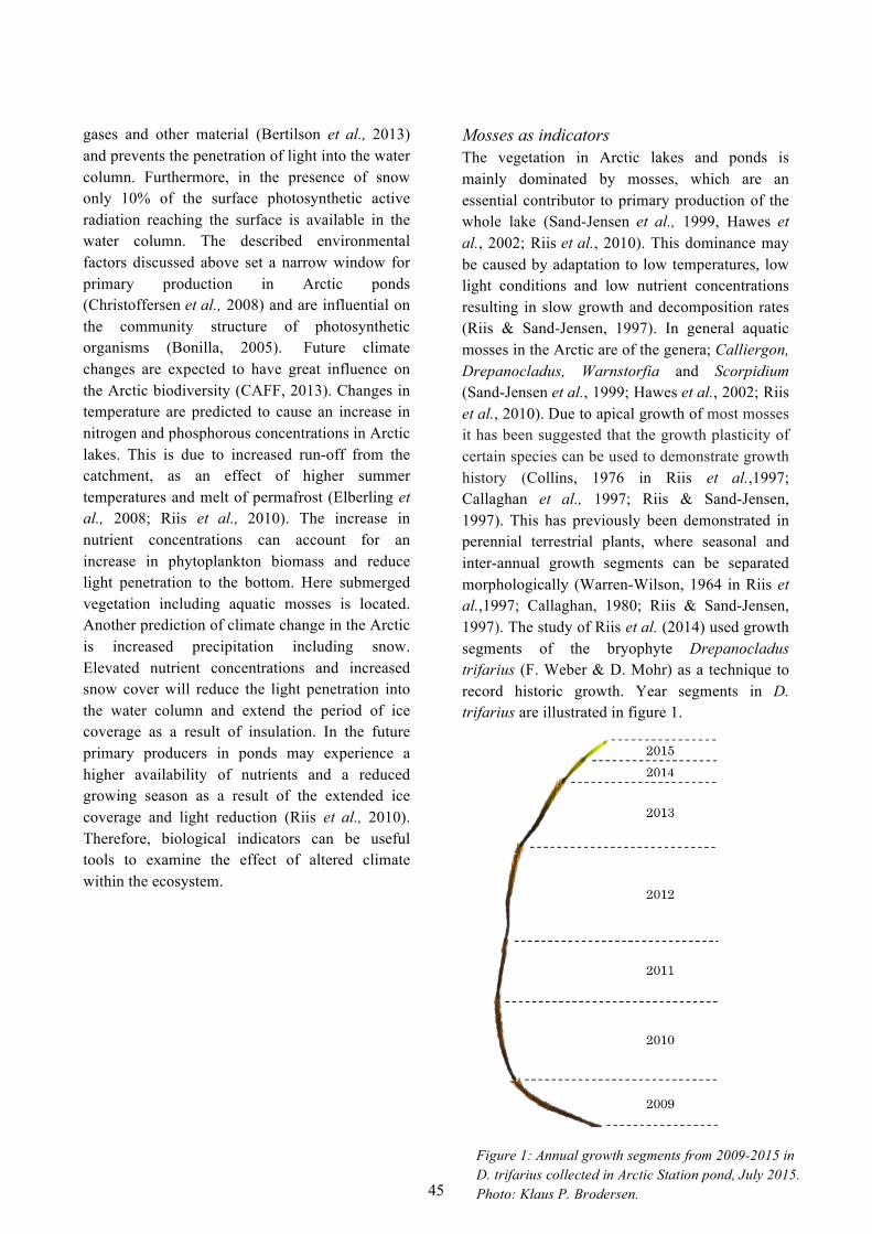
gases and other material (Bertilson et al., 2013) and prevents the penetration of light into the water column. Furthermore, in the presence of snow only 10% of the surface photosynthetic active radiation reaching the surface is available in the water column. The described environmental factors discussed above set a narrow window for primary production in Arctic ponds (Christoffersen et al., 2008) and are influential on the community structure of photosynthetic organisms (Bonilla, 2005). Future climate changes are expected to have great influence on the Arctic biodiversity (CAFF, 2013). Changes in temperature are predicted to cause an increase in nitrogen and phosphorous concentrations in Arctic lakes. This is due to increased run-off from the catchment, as an effect of higher summer temperatures and melt of permafrost (Elberling et al., 2008; Riis et al., 2010). The increase in nutrient concentrations can account for an increase in phytoplankton biomass and reduce light penetration to the bottom. Here submerged vegetation including aquatic mosses is located. Another prediction of climate change in the Arctic is increased precipitation including snow. Elevated nutrient concentrations and increased snow cover will reduce the light penetration into the water column and extend the period of ice coverage as a result of insulation. In the future primary producers in ponds may experience a higher availability of nutrients and a reduced growing season as a result of the extended ice coverage and light reduction (Riis et al., 2010). Therefore, biological indicators can be useful tools to examine the effect of altered climate within the ecosystem.
Mosses as indicators The vegetation in Arctic lakes and ponds is mainly dominated by mosses, which are an essential contributor to primary production of the whole lake (Sand-Jensen et al., 1999, Hawes et al., 2002; Riis et al., 2010). This dominance may be caused by adaptation to low temperatures, low light conditions and low nutrient concentrations resulting in slow growth and decomposition rates (Riis & Sand-Jensen, 1997). In general aquatic mosses in the Arctic are of the genera; Calliergon, Drepanocladus, Warnstorfia and Scorpidium (Sand-Jensen et al., 1999; Hawes et al., 2002; Riis et al., 2010). Due to apical growth of most mosses it has been suggested that the growth plasticity of certain species can be used to demonstrate growth history (Collins, 1976 in Riis et al.,1997; Callaghan et al., 1997; Riis & Sand-Jensen, 1997). This has previously been demonstrated in perennial terrestrial plants, where seasonal and inter-annual growth segments can be separated morphologically (Warren-Wilson, 1964 in Riis et al.,1997; Callaghan, 1980; Riis & Sand-Jensen, 1997). The study of Riis et al. (2014) used growth segments of the bryophyte Drepanocladus trifarius (F. Weber & D. Mohr) as a technique to record historic growth. Year segments in D. trifarius are illustrated in figure 1.
Figure 1: Annual growth segments from 2009-2015 in D. trifarius collected in Arctic Station pond, July 2015. Photo: Klaus P. Brodersen. 45

This method was validated by comparing growth segments with the growth of mosses grown in situ for one year. Additionally their study showed an influence of different climatic conditions on annual growth. With bryophytes being the most abundant primary producer in Arctic lakes and ponds, it can be a useful organism to use as an indicator of altered climate in the Arctic.
Drepanocladus trifarius D. trifarius is a semi-aquatic bryophyte occurring in well-lit and constantly moist, wet or submerged habitats. It is most frequently found in weakly acidic to sub-neutral habitats. Most Arctic lakes where bryophytes are distributed remain nutrient-poor, although they can also inhabit nutrient-rich regions (Hedenäs & Bisang, 2012). The occupied niche of D. trifarius concerning nutrients and pH is therefore quite broad, and climatic conditions such as temperature and light may be a more influential factor for the growth of the bryophyte. However, there have only been few studies evaluating aquatic mosses in the Arctic and there has been no overall consensus about how growth segments in aquatic mosses can be used as an appropriate indicator for altered climate, why further studies has to be conducted (Bisang et al. 2008).
In this study we analyse annual growth of D. trifarius (F. Weber & D. Mohr) in two Arctic ponds and relate the net production to environmental and climatic factors. We expect the growth of D. trifarius to increase with higher mean summer temperature and larger net-
radiation in ice-free periods. Finally we expect growth to decrease with prolonged ice-coverage and increased maximal snow-depth.
Study site The study was conducted in the period of the 7th to the 17th July 2015 in two small ponds at Disko, West Greenland (69° 16’ 13’ N’, 53 28’ 34’’ W); one pond is located behind the Arctic Station in Qeqertarsuaq (69° 15’ 13” N, 53° 31’ 29” W) and the second pond in the area of Kangaarsuk (69° 15’ 59” N, 53° 49’ 42” W) (figure 2). The ponds hereafter called Arctic Station pond and Kangaarsuk pond are small and shallow (213 m2, mean depth 23 ± 12 cm; 1151 m2, mean depth 36 ± 28 cm respectively). D. trifarius was found in Arctic Station pond previously in 1962 (Røen, 1962). Both ponds are ice-free during summer (in this study defined as 1th June to 30th September) and freeze solid in winter (based on data from Arctic Station Automatic Weather Station). Both ponds are fishless and receive water from snowmelt in the catchment and have no anthropogenic disturbance. They are located near the coast: Arctic Station pond is situated on a plateau (Altitude: 35 m.a.s.l.), whereas Kangaarsuk pond is on a small peninsula and thus more exposed to the sea (Altitude: 17 m.a.s.l.).
Methods Physical and chemical conditions Water samples for chlorophyll a, total nitrogen (TN), total phosphorous (TP), pH and alkalinity were collected in a 5 L bottle and returned to the
Figure 2: Location map of Disko, Greenland. The two study sites are located at the southern part of Disko. Left: Kangaarsuk pond: 1151 m2. Right: Arctic Station: 213 m2 (From NunaGIS).
46

laboratory for further analysis.
Conductivity was measured using a conductivity meter (LF 340, WTW, Germany). Light extinction and diurnal variation in temperature were measured in Arctic Station pond with HOBO-loggers mounted above and under the water surface in two depths. Each HOBO-logger had prior to mounting been inter-calibrated to a PAR-sensor (Quantum sensor LI-190, Li-cor Biosciences, UK) and individual LUX to PAR conversion factors calculated by linear regression. Due to lack of matching time points in the light measurements the light extinction coefficients were calculated based on mean light intensities measured by the HOBO-loggers during the period. Due to technical problems, it was not possible to measure and calculate light extinction coefficient in Kangaarsuk pond. The areas of the ponds were measured with an area tool in NunaGIS. Three transects (25%, 50% and 75% of the pond width) were made across the ponds to determine mean depth and frequency of substrates, categorized as moss, rock, mud, mire or terrestrial plants. In the laboratory water samples for TN and TP analyses were poured in 100 ml vials and kept frozen until the return at Freshwater Biological Laboratory, University of Copenhagen. Here samples were thawed and analysed for TN and TP with a SEAL AutoAnalyzer 3 HR according to standard method (modified from Limnologisk metodik, Ferskvandsbiologisk Laboratorium, 1977). pH were measured with a standard pH meter (pHM 210, MeterLab, Radiometer analytical). Water for determination of chlorophyll a content was filtered on a 47 mm GFC filter in triplicates and frozen until the return to Denmark. Here chlorophyll α (µg l-1) were determined by overnight ethanol extraction according to Jespersen & Christoffersen (1987) and measured on a spectrophotometer (Shimadzy UV spectrophotometer. UV-1800). Total alkalinity was determined by titration with 0.1 M HCl to pH
4.7 (modified from Limnologisk metodik, Ferskvandsbiologisk Laboratorium, 1977). Reconstruction of annual growth D. trifarius was present in both Arctic Station pond and Kangaarsuk pond and was only found in the shallower parts. Species identification has been confirmed by Kristian Hassel (Natural History University Museum, Norges teknisk-naturvitenskapelige universitet, Tronheim), Irene Bisang and Lars Hedenäs (both Swedish Museum of Natural History, Stockholm). In Kangaarsuk D. trifarius was found between dense stands of Scorpidium scorpioides (Hedw.) Limpr. A list of additional finding locations is found in appendix 1. The shoots of D. trifarius’ annual growth segments can be distinguished visually by the clear separation of parts consisting of short and closely spaced leaves separated by parts with longer and more distinct leaves. The most recent annual shoot appears bright green in colour (figure 3) (Riis et al., 2014).
Figure 3: Separation of growth segments in D. trifarius. Node starts a new segment and spaced leaves indicate the apical part of the shoot. Photo: Klaus P. Brodersen. Random sampling of the mosses was performed, and 100 individuals from each study site were collected and transported to the laboratory for further analyses. In total 100 individuals with 587 segments were sampled in Arctic Station pond and 100 individuals with 517 segments in Kangaarsuk pond. We chose to incorporate individuals from 2009-2014 in the further analysis to secure a full growth season and sufficient replicates. As far as possible, mosses without branches were selected for measurements. If a moss had a branch, which that was clearly of this year growth,
47

the branch was dismantled and marked as part of the annual segment. 17 individuals of D. trifarius had side branches in Kangaarsuk pond compared to one individual in Arctic Station pond. The effect of side branches on annual growth has been taken into consideration in the analysis, and the effect of branching was tested with a two-way ANOVA with year and side-branches as different factors. In the laboratory, shoots of D. trifarius were gently brushed to remove epiphytes prior to handling. The layer of epiphytes on D. trifarius was visually estimated to be greater in Kangaarsuk pond, but no measurement was made. For each moss individual, the length of the annual segments was measured to the nearest half millimetre using a stereoscopic microscope (Olympus Model SZX12- IllK200, Nikon Model SMZ1B). Annual segments were dried in an oven at 60 °C for 24 hours. Biomass (mg DW) of each segment was weighed with a microbalance (Mettler AT261 DeltaRange) to the nearest 0.01 mg.
Climate data Climate data from 2009-2014 was provided by Arctic Station (Automatic Weather Station AWS-1. 69° 15' 11" N, 53° 31' 13" W, 24 m.a.s.l). Inthis study we use daily average measurements of air temperature (°C), precipitation (mm) and in- and outgoing radiation (W m-2). The summer period was defined from 1th June to 30th September, and from this period the mean summer temperature was calculated. Frost days were defined as number of days with temperature below 0°C and used to indicate the period where the ponds were covered by ice, and thus a reduction in incoming radiation. Snow depth (cm) was measured daily by the Arctic Station personnel as a part of the stations monitoring programme. Since the Weather Station measures 2-9.5 m above terrain and is not located next to the ponds, climate data will only be a proxy for the climatic conditions in the ponds. Values of climatic conditions are shown in appendix 2.
Data analysis We used one-way ANOVA and Bonferonni as post hoc to test for differences between annual growth segments. The assumptions for using ANOVA, variance homogeneity and normal distribution of data, were tested with Bartlett's test and D'Agostino test, respectively. At the time of sampling, annual growth segments from 2015 was incomplete and therefore not included in any statistical analyses. Difference in annual segment length, biomass and the effect of ponds were tested using a two-way ANOVA. Impact of side branches on annual growth was also tested using a two-way ANOVA. Finally relationship between annual segments (length and weight) and environmental and climatic data (net radiation, snow depth, summer temperature, length of ice-coverage and precipitation) were tested with Pearson Production Moment correlation. Significant correlations were tested with linear regression. Confidence interval was at a 95% level. All statistical analyses were performed using GraphPad Prism, version 6.0.
Results Physical and chemical conditions Arctic Station pond and Kangaarsuk pond are both nutrient-poor, clear-water ponds with a low concentration of chlorophyll a, indicating a limited biomass of phytoplankton (table 1). The two ponds differ in size, mean depth, conductivity and substrate distribution (%). The sheer size and depth of the pond in Kangaarsuk is larger compared to Arctic Station pond. A higher proportion of moss as substrate was found in Kangaarsuk pond, and here D. trifarius was found between high densities of S. scorpioides. Conductivity varied between the two ponds with the highest levels in Kangaarsuk pond, suggesting a higher amount of dissolved inorganic compounds in the water, which may originate from the greater marine exposure. The light extinction coefficient was calculated to be 3.2 m-1 for Arctic Station pond. This means that, with a mean depth of 23.3 (± 11.8) cm, light is present
48

through the whole water column. In Arctic Station pond diurnal fluctuations in temperature were large, ranging from 9.3 °C to 21.5 °C. All values are present in table 1.
Annual growth segments and climatic conditions Annual growth segments were identified up to 22 years in one D. trifarius individual, but for most of the individuals only the past 6 years were sampled (figure 4). In Arctic Station pond average growth year-1 across segments from 2009 to 2014 was 2.47 ± 0.31 cm year-1 with corresponding biomass 2.56 ± 0.39 mg DW year-1. In Kangaarsuk pond average annual segment length was 1.76 ± 0.34 cm with a corresponding biomass of 1.53 ± 0.29 mg DW. Inter-annual variation
occurred in both Arctic Station pond and Kangaarsuk pond, and in both ponds annual growth segment from 2012 was significantly larger (One-way ANOVA, P<0.0001, n=100) (figure 4), suggesting better conditions for growth in 2012. Some individuals of D. trifarius sampled from Kangaarsuk pond showed many side branches (17 individuals), assumed to originate from overgrowth with S. scorpioides. No significant effect of side branches on the mean length of the mosses was found (Df=1, P=0.5415), but instead a significant effect of year (Df=5, P<0.0001). In addition, no significant effect of side branches on mean biomass was found (Df=1, P=0.4654), why including all individuals from Kangaarsuk in further analysis seems reasonably. The relationship between climatic factors and annual growth segments was tested with Pearson Product Moment Correlation. When correlating the mean length of annual growth segments with different climatic conditions, a positive relationship between annual growth segments and mean summer temperature was found in both
Mean values (± SD) Arctic Station pond
Kangaarsuk pond
Mean depth (cm) 23.3 (± 11.8)
36.3 (± 27.6)
Mean water temp (°C) 13.1(± 5.3) 13.6
Substrate (%) Moss Rock Mud Mire Terrestrial plants
21.6 62.2 10.8 5.4 0
35.6 45.2
0 15.1 4.1
pH 7.7 7.32
Conductivity (µS cm-1) 13 (±1) 66
Alkalinity (meq l-1) NA 0.09
Chlorophyll α (µg l-1) 0.39 0.54
TN (µg l-1) 401.33 544.91
TP (µg l-1) 8.38 6.86
Figure 4: Mean annual segment biomass (DW) (A, B) and length (cm) (C,D) in D. trifarius collected in Arctic Station pond and Kangaarsuk pond, Disko, in July 2015. Error bars indicate ± SD and letters indicate significant differences between years (one-way ANOVA, F=16-39, P<0.0001, n=17-100, Df=5).
Table 1: Environmental parameters for Arctic Station pond and Kangaarsuk pond, measured July 2015. NA indicates that data was not available. Mean values (± SD).
49

Arctic Station pond and Kangaarsuk pond (figure 5A and 5B). This indicates, that with a higher temperature the longer the annual growth segment. Using linear regression, mean summer temperature explains 86% of the variation in length of the annual growth segments in Arctic Station pond (Linear regression, P=0.007) and 77% in Kangaarsuk pond (Linear regression, P = 0.021). Same trend was seen with biomass (DW), but no correlations were significant (figure 5G and 5H). This suggests that biomass of D. trifarius may depend on factors other than temperature; possibly epiphyte growth, degradation with age and potentially herbivory. Therefore, we chose not to consider the biomass measurements in our further analysis.
In contrast to predictions, no significant relationship existed when correlating annual length and annual biomass with net-radiation in June (figure 5C and 5D), frost days (figure 5E and 5F), in- and outgoing radiation and snow depth (appendix 3). Even though relationships were non-significant, a tendency was seen between outgoing radiation and the length of annual growth segments from Kangaarsuk pond. Here 56% (90% confidence interval) of the variation in length of the annual growth segments was explained by outgoing radiation. All correlation coefficients are present in table in appendix 3.
In general absolute measurements of length (cm) were larger in individuals from Arctic Station pond compared to Kangaarsuk pond. To allow a comparison between annual segment length and biomass between the two ponds, the relative growth year-1 as a percentage of the total length of the moss from 2010-2014 was calculated (figure 6). This showed that, D. trifarius from Kangaarsuk pond in 2012 grew relatively faster than in Arctic Station pond, 35% and 27% respectively. The SD of relative growth was generally higher in Kangaarsuk than Arctic Station pond, ranging 3.6-8.0% and 3.2-4.5% respectively. The higher SD values in Kangaarsuk
pond indicate more heterogenic conditions within the pond.
We tested if relative growth in the two ponds was significantly different and if the pond itself showed an effect on the relative length. A two-way ANOVA showed a significant effect of year (Df=4, P<0.0001) as well as of the “pond” (Df=1, P<0.0001) on the relative lengths. This suggests that the environment in the pond affects the growth of these mosses and they do not respond equally to climatic conditions.
Figure 6: Relative length (%) of annual growth segments in Arctic Station pond and Kangaarsuk pond. Error bars indicate ±SD.
50

Figure 5: Relationships between climatic conditions and mean annual growth segment in D. trifarius from Arctic Station pond (right column) and Kangaarsuk pond (left column). Figure A-F show relationship between environmental factors and annual length and G-H show relationship with biomass. * indicates significant relationship P<0.05 and *NS indicates a non significant correlation. Error bars indicate ±SD.
51

Discussion Differences in growth The growth reconstruction technique of D. trifarius allowed determination of annual growth segments up to 22 years back. A period from 2009-2014 was chosen for further analysis, to secure a large and more even numbers of replicates. Length and weight of annual growth segments were comparable to other studies of annual growth in aquatic mosses in the Arctic and Subarctic regions; D. trifarius in Lake Sommerfuglesø (Riis et al. 2014), D. revolens var. intermedius in Char Lake (Sand-Jensen et al. 1999), C. gigantheum in Colour Lake (Hawes et al. 2002) and D. trifarius from northern Lappmark (Bisang et al. 2008).
We found individuals from Arctic Station pond were generally larger compared to Kangaarsuk pond and when comparing the growth of the mosses from the years 2009-2014, we found that D. trifarius grew significantly slower in Kangaarsuk pond compared to Arctic Station pond. These findings suggest better conditions for growth of D. trifarius in Arctic Station pond compared to Kangaarsuk pond. The effects might be due to different environmental conditions in the two ponds as the presence of S. scorpioides in Kangaarsuk pond. S. scorpioides is known to inhabit more mineral-rich habitats (Hedenäs & Eldenäs 2008), which is consistent with the higher conductivity that we found in Kangaarsuk pond (66 µS cm-1). In addition elevated salinity and conductivity levels will occur during the ice-in period, which might favour growth of S. scorpioides even more.
Correlation to climatic conditions Despite the difference in growth rate in D. trifarius between Arctic Station pond and Kangaarsuk pond, the between-year differences were significantly different in both ponds, where segments from 2012 were greater than previous years. This is in contrast to the study of Sand-Jensen et al. (1999) where no between-year
variations were found. The authors suggest that this result is due to low variation in climatic conditions. The climate conditions at our locations in 2009-2014 varied significantly (see appendix 2 for exact values). This variation in climate may be useful as a proxy for bryophyte growth.
When correlating length to climatic conditions, temperature could explain 77% and 86% of the between-year variation of annual growth segments in Kangaarsuk pond and Arctic Station pond respectively. This is similar to studies of Callaghan et al. (1997), who found a positive relationship between temperature and growth in Hylocomium splendens (Hedw.) Br. Eur. The relationship between length and temperature was found to be positive, with temperature as a determining factor for growth.
An interesting observation was found when comparing the relative growth of the mosses. Here we found that Kangaarsuk pond had a higher variation between years than in Arctic Station pond (figure 6). Growth segments from the year 2012 made out 35% of the total length (year segments from 2010-2014) in Kangaarsuk pond and 27% in Arctic Station pond. Even though temperature shows good correlation with the different annual growth segments, the larger relative variance in years found in Kangaarsuk pond could indicate that growth is determined by other conditions than climate. Here we hypothesize the presence of S. scorpiodes to have an influence on the growth. The high abundance of S. scorpioides may have resulted in unstable conditions for growth in Kangaarsuk pond. If there were less favourable conditions for S. scorpioides in 2012, there may have been more space and less competition to promote D. trifarius. The increased climatic stability and reduced competition in Arctic Station pond may have resulted in increased growth.
We hypothesized that altered light conditions would affect growth segments of D. trifarius. As described in the introduction a reduction in light
52

will occur when ice- and snow coverage is prolonged. Contrary to our expectation and the study of Riis et. al. (2014), the growth segments of D. trifarius did not correlate directly to frost days and maximum snow depth. This picture could have been blurred by the fact that the measured incoming light does not represent the light regime in the pond. Moreover, only in cases of high number of frost days will ice coverage limit penetration of light into the water column. Additionally the former study of McIntire et al. (1994) showed that mosses can survive at 0.1-2% of surface irradiance (McIntire et al. 1994 in Hawes et al. 2002). Our findings also support the results from the study of Hawes et al. (2002), where persistence of ice coverage had no relation to length of the growth segments. Hawes et al. (2002) have previously questioned length of mosses as an indicator of growth, since moss stems have the ability to etiolate under low-light conditions (Priddle 1980a in Hawes et al. 2002). Thus bryophyte stems can elongate under ice coverage and annual segments can therefore be longer as a response to low light. However, ponds are expected to freeze solid during winter and therefore photosynthesis in the mosses decreases and growth stops. Thus elongation may not be the reason for the low explanatory coefficients. When correlating climatic conditions with biomass (DW) no significant relationships were found, thus biomass seems a less suitable descriptor of growth. The poor correlations with biomass may be caused by epiphyte growth on the mosses. Extensive epiphyte growth was observed on Kangaarsuk individuals and as epiphytes can exert massive shading on the mosses and competition for light it may have impact on the biomass (Sand-Jensen, 1977). Also the ability of D. trifarius to reallocate nutrients from older year segments to new growth may have an impact on the biomass and may be the reason for the low explanatory coefficients. Given the low level of concordance between annual growth segments and environmental conditions with measurements of both length and biomass, it is essential to
evaluate if D. trifarius is an appropriate indicator for altered climate.
Challenges of using D. trifarius as an indicator for altered climate Side branches Another challenge with using D. trifarius as a biological indicator is that it produces side branches. Currently there exists little guidance on how to overcome this problem. Side branches are assumed to increase the variation in-between samples by focusing growth in two directions instead of one, and thereby lower the direct response to altered climate. It is very difficult to know exactly which year the side branch is from. Therefore including them will increase the variation in the measurements. Therefore we would expect growth measured as length to be lower in individuals with side branches. From Kangaarsuk we sampled 17 individuals with side branches out of 100. We tested the effect of including the individuals with side branches in our analyses compared to excluding them. There was no significant effect of including the individuals with side branches, and thus we have included all individuals in our analyses. The fact that it was only 17 individuals with side branches out of 100 could have an impact on the conclusion of the significance, but for this study it did not affect our results. Reallocation Even though bryophytes are nonvascular organisms, evidence exists that D. trifarius possess the advantage of resource allocation (Bisang et al. 2008, Riis et al. 2014). This may affect the productivity in the individual annular segments, and influence annual growth (Bisang et al. 2008). Studies have also been made for other bryophytes, where the nutrient content in segments of every age and depth was low, but the content of carbon, nitrogen and phosphorous was higher in the youngest apical segments (Sand-Jensen et al., 1999). This trait is a big advantage in oligotrophic conditions, and sets back the
53
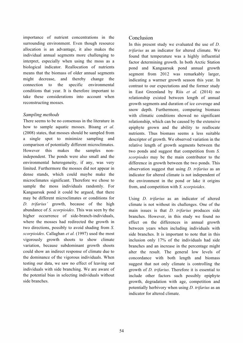
importance of nutrient concentrations in the surrounding environment. Even though resource allocation is an advantage, it also makes the individual annual segments more challenging to interpret, especially when using the moss as a biological indicator. Reallocation of nutrients means that the biomass of older annual segments might decrease, and thereby change the connection to the specific environmental conditions that year. It is therefore important to take these considerations into account when reconstructing mosses.
Sampling methods There seems to be no consensus in the literature in how to sample aquatic mosses. Bisang et al. (2008) states, that mosses should be sampled from a single spot to minimize sampling and comparison of potentially different microclimates. However this makes the samples non-independent. The ponds were also small and the environmental heterogeneity, if any, was very limited. Furthermore the mosses did not appear in dense stands, which could maybe make the microclimates significant. Therefore we chose to sample the moss individuals randomly. For Kangaarsuk pond it could be argued, that there may be different microclimates or conditions for D. trifarius’ growth, because of the high abundance of S. scorpioides. This was seen by the higher occurrence of side-branch-individuals, where the mosses had redirected the growth in two directions, possibly to avoid shading from S. scorpioides. Callaghan et al. (1997) used the most vigorously growth shoots to show climate variation, because subdominant growth shoots could show an indirect response of climate due to the dominance of the vigorous individuals. When testing our data, we saw no effect of leaving out individuals with side branching. We are aware of the potential bias in selecting individuals without side branches.
Conclusion In this present study we evaluated the use of D. trifarius as an indicator for altered climate. We found that temperature was a highly influential factor determining growth. In both Arctic Station pond and Kangaarsuk pond annual growth segment from 2012 was remarkably larger, indicating a warmer growth season this year. In contrast to our expectations and the former study in East Greenland by Riis et al. (2014) no relationship existed between length of annual growth segments and duration of ice coverage and snow depth. Furthermore, comparing biomass with climatic conditions showed no significant relationship, which can be caused by the extensive epiphyte grown and the ability to reallocate nutrients. Thus biomass seems a less suitable descriptor of growth. We observed variation in the relative length of growth segments between the two ponds and suggest that competition from S. scorpiodes may be the main contributor to the difference in growth between the two ponds. This observation suggest that using D. trifarius as an indicator for altered climate is not independent of the environment in the pond or lake it origins from, and competition with S. scorpioides.
Using D. trifarius as an indicator of altered climate is not without its challenges. One of the main issues is that D. trifarius produces side branches. However, in this study we found no effect on the differences in annual growth between years when including individuals with side branches. It is important to note that in this inclusion only 17% of the individuals had side branches and an increase in the percentage might alter the result. The general low levels of concordance with both length and biomass suggest that not only climate is controlling the growth of D. trifarius. Therefore it is essential to include other factors such possibly epiphyte growth, degradation with age, competition and potentially herbivory when using D. trifarius as an indicator for altered climate.
54

Acknowledgments We want to thank the staff at Arctic Station for providing climate data, Tenna Riis (University of Aarhus) for inspiration to the project and guidance in sampling of mosses, Klaus P. Brodersen for providing photos of high quality and Tom Bean for review this study. We are grateful to Kristian Hassel (Natural History University Museum, Norges teknisk-naturvitenskapelige Universitet, Tronheim), Irene Bisang and Lars Hedenäs (Both Swedish Museum of Natural History, Stockholm) for their assistance with identifying D. trifarius. Finally, we are grateful to Professor Kirsten S. Christoffersen for guidance during the planning of this study, during fieldwork and for the editorial assistance. References Bertilsson, S., Burgin, A., Carey, C.C., Fey, S.B.,
Grossart, H.-P., Grubisic, L.M., Jones, I.D., Kirillin, G., Lennon, J.T., Shade, A. & Smyth, R.L., 2013. The under-ice microbiome of seasonally frozen lakes. Limnology and Oceanography, 58, 1998-2012.
Bisang, I., Ehrlen, J., & Hedenäs, L.,2008. Are annual
growth intervals independent units in the moss Pseudocalliergontrifarium(Amblystegiaceae). Bryologist, 111, 435-443.
Bonilla, S., Villeneuve, V. & Vincent, W.F.,2005.
Benthic and planktonic algal communities in a High Arctic Lake: Pigment structure and contrasting responses to nutrient enrichment. Journal of Phycology, 41, 1120-1130.
Bolsenga, S.J. & Vanderploeg H.A.,1992. Estimating
photosynthetically available radiation into open and ice-covered fresh-water lakes frim surface characteristics – a high transmittance case-study. Hydrobiologia, 24, 95-104.
Callaghan, T.V., Carlsson, B.A., Sonesson, M. &
Temesváry, A.,1997. Between-year variation in climate-related growth of circumarctic populations of the moss Hylocomium splendens. Functional Ecology, 11, 157-165.
Callaghan, T.V.,1980. Age-related patterns of nutrient allocation in Lycopodiuman notinum from Swedish Lapland. Oikos, 35, 373-386.
CAFF,2013. Arctic Biodiversity Assessment. Status
and trends in Arctic biodiversity. Conservation of Arctic Flora and Fauna, Akureyri.
Christoffersen, K.S., Amsinck, S.L., Landkildehus, F.,
Lauridsen, T.L., & Jeppesen, E.,2008. Lake flora and fauna in relation to ice-melt, water temperature and chemistry at Zackenberg. Advances in Ecological Research, 40, 371-389.
Collins, N.J.,1976. Growth and population dynamics of
the moss Polytrichumal pestre in the maritime Antarctic. Oikos, 27, 389-401.
Elberling, B., Tamstorf, M.P., Michelsen, A., Arndal,
M.F., Sigsgaard, C., Illeris, L. & Beyens, L.,2008. Soil and plant community-characteristics and dynamics at Zackenberg. Advances in Ecological Research, 40, 223-248.
Ferskvandsbiologisk Laboratorium, Københavns
Universitet,1977. Limnologisk Metodik, Akademisk Forlag, 2. udgave. pp. 27-43.
Hawes, I., Andersen, D.T. & Pollard, W.H.,2002.
Submerged Aquatic Bryophytes in Colour Lake, a Naturally Acidic Polar Lake with Occasional Year-Round Ice-Cover. Arctic, 55, 380-388.
Hedenäs, L., & Bisang, I.,2012. Drepanocladus
trifarius - an example of unsuspected niche widths among mosses. Nordic Journal of Botany, 30, 747-753.
Hedenäs, L. & Eldenas, P.,2008. Relationship in
Scorpidium (Calliergonaceae, Bryophyta), especially between S. cossonii and S. scorpioides, Taxon, 57. 121-130.
Jespersen, A. M., & Christoffersen, K.,1987.
Measurements of chlorophyll-a from phytoplankton using ethanol as extraction
55

solvent. Archiv Fur Hydrobiologie, 109, 445-454.
Kling, G. W.,2009. Lakes of the Arctic. Pages 577–588 in G. E. Likens (ed.). Encyclopedia of Inland Waters. Elsevier, Oxford.
Lacoul, P. & Freedman, B.,2006. Environmental influences on aquatic plants in freshwater ecosystems. Environmental reviews, 14, 89-136.
McIntire, C.D., Phinney, H.K., Larson, G.L., and Buretenica, M.,1994. Vertical distribution of a deep-water moss and associated epiphytes in Crater Lake, Oregon. Northwest Sci, 68,11–21.
Priddle, J.,1980a. The production ecology of benthic plants in some Antarctic lakes. Journal of ecology. 68, 141-153.
Rautio, M., Dufresne, F., Laurion, I., Bonilla, S., Vincent, W.F., & Christoffersen, K.S.,2011. Shallow freshwater ecosystems of the circumpolar Arctic. Ecoscience, 18, 204-222.
Riis, T., Christoffersen, K.S., & Baattrup-Pedersen, A.,2014. Effects of warming on annual production and nutrient-use efficiency of aquatic mosses in a high Arctic lake. Freshwater Biology, 59, 1622-1632.
Riis, T., Olesen, B., Katborg, C.K., & Christoffersen, K.S.,2010. Growth Rate of an Aquatic Bryophyte (Warnstorfia fluitans (Hedw.) Loeske) from a High Arctic Lake: Effect of Nutrient Concentration. Arctic, 63, 100-106.
Riis, T., & Sand-Jensen, K.,1997. Growth reconstruction and photosynthesis of aquatic mosses: Influence of light, temperature and carbon dioxide at depth. Journal of Ecology, 85, 359-372.
Røen, U. I.,1962. Studies on Freshwater Entomostraca in Greenland - Localities, Ecology and Geographical Distribution of the Species.Meddelelser om Grønland bd.170, No.2, pp. 83.
Sand-Jensen, K., Riis, T., Markager, S., & Vincent, W.F.,1999. Slow growth and decomposition of mosses in Arctic lakes. Canadian Journal of Fisheries and Aquatic Sciences, 54, 388-393.
Sand-Jensen.,1977. Effect of epiphytes on eelgrass photosynthesis. Aquatic botany 3, 55-53.
Vincent W.F & Laybourn-Parry J.,2008. Polar Lakes and Rivers. Limnology of Arctic and Antarctic Aquatic Ecosystems. Oxford University Press. 157-196
Warren-Wilson, J.,1964. Annual growth of Salix arctica in the high-arctic. Annals of Botany, 109, 71-76.
56

Appendix 1: Findings of Drepanocladus trifarius Drepanocladus trifarius
Findings are not verified. Kangaarsuk pond: Lat 69° 15’ 59” N Lon 53° 49’ 42” W Altitude (ft): 56 Ilulissat: Lat 69° 16’ 02” N Lon 53° 48’ 58” W Altitude (ft): 15 Qeqertarsuaq: Near Engelskmandshavn Lat 69° 15’ 20” N Lon 53° 32’ 26” W Altitude (ft): 97 Plateau behind Arctic Station: Pond 1 Lat 69° 15’ 17” N Lon 53° 31’ 22” W Altitude (ft): 110 Pond 2 Lat 69° 15’ 14” N Lon 53° 31’ 24” W Altitude (ft): 108 Coffee pond Lat 69° 15’ 14” N Lon 53° 31’ 25” W Altitude (ft): 134 Arctic Station pond Lat 69° 15’ 13” N Lon 53° 31’ 29” W Altitude (ft): 116 After coffee pond Lat 69° 15’ 13” N Lon 53° 31’ 32” W Altitude (ft): 85
57

App
endi
x 2.
Clim
atic
con
ditio
ns m
easu
red
at A
rctic
Sta
tion’
s A
utom
atic
Wea
ther
Sta
tion
AW
S (1
69°
15'1
1.0"
N. 5
3°31
'13.
0". 2
4 m
asl
). Su
mm
er is
de
fined
as
the
perio
d fr
om 1
th J
une
to 3
0th S
epte
mbe
r and
fros
t day
s as
num
ber o
f day
s w
ith te
mpe
ratu
re b
elow
0°C
.
Mea
n su
mm
er a
ir
tem
p. (°
C. 2
00
cm)
Mea
n ye
ar te
mp.
(°
C. 2
00 c
m)
Mea
n su
mm
er
prec
ipita
tion
(mm
Wat
er E
Q)
Yea
r pr
ecip
itatio
n (m
m
Wat
er E
Q)
Fros
t day
s (t
emp
<0 °C
) M
ax. s
now
dep
th
(cm
)
Inco
mi n
g sh
ortw
ave
radi
atio
n an
nual
mea
n
Out
goin
g sh
ortw
ave
radi
atio
n an
nual
mea
n (W
m-2
)
Net
rad
iatio
n an
nual
mea
n (W
m-2
)
(W m
-2)
2009
6.
55
-2.2
N
A
NA
21
6 23
13
1 40
91
2010
7.
79
1.0
1.47
1.
01
162
48
117
NA
N
A
2011
6.
57
-2.6
N
A
NA
23
2 32
11
8 39
79
2012
7.
84
-2.2
1.
64
0.85
19
9 25
11
5 28
86
2013
6.
21
-1.8
1.
08
0.49
21
4 32
12
1 26
95
2014
6.
56
-1.9
2.
01
0.77
21
3 50
11
8 33
85
Inco
mi n
g sh
ortw
ave
radi
atio
n su
mm
er m
ean
(W m
-2)
Out
goin
g sh
ortw
ave
radi
atio
n su
mm
er m
ean
(W m
-2)
Net
rad
iatio
n su
mm
er m
ean
(W m
-2)
Mea
n Ju
ne a
ir te
mp.
(°
C. 2
00 c
m)
Mea
n Ju
ne
prec
ipita
tion
(mm
Wat
er E
Q)
Inco
mi n
g sh
ortw
ave
radi
atio
n Ju
ne
(W m
-2)
Out
goin
g sh
ortw
ave
radi
atio
n Ju
ne
(W m
-2)
Net
rad
iatio
n Ju
ne
(W m
-2)
225
29
196
5.14
N
A
287
30
257
197
23
173
6.23
N
A
252
29
223
201
27
174
5.41
N
A
277
40
237
194
21
174
8.07
N
A
294
33
261
205
22
183
6.27
N
A
298
29
268
196
22
174
6.57
N
A
277
28
250
*NA
indi
cate
s da
ta n
ot a
vaila
ble
58

App
endi
x 3.
Pea
rson
s Pro
duct
Mom
ents
Cor
rela
tion
coef
ficie
nts f
rom
cor
rela
tion
of d
iffer
ent e
nviro
nmen
tal c
ondi
tions
to a
nnua
l seg
men
t le
ngth
and
bio
mas
s in
D. t
rifa
rius
from
Arc
tic S
tatio
n po
nd a
nd K
anga
arsu
k po
nd. S
umm
er is
def
ined
as t
he p
erio
d fr
om 1
th Ju
ne to
30th
Se
ptem
ber a
nd fr
ost d
ays a
s num
ber o
f day
s with
tem
pera
ture
bel
ow 0
°C.
Mea
n su
mm
er
air
tem
p.
(°C
. 200
cm
)
Mea
n ye
ar te
mp.
(°
C. 2
00 c
m)
Mea
n su
mm
er
prec
ipita
tion
(mm
Wat
er E
Q)
Yea
r pr
ecip
itatio
n (m
m W
ater
EQ
)
Fros
t day
s (t
emp
<0 °C
) M
ax. s
now
dep
th
(cm
)
Inco
min
g sh
ortw
ave
radi
atio
n A
nnua
l mea
n
(W m
-2)
Out
goin
g sh
ortw
ave
radi
atio
n A
nnua
l mea
n (W
m-2
)
Arc
tic S
tatio
n po
nd
Len
gth
0.86
*0.
070.
030.
420.
330.
010.
290.
17D
W
0.64
**0.
160.
010.
160.
140.
130.
290.
15
Kan
gaar
suk
pond
L
engt
h0.
77*
0.08
0.72
0.72
0.29
0.08
0.17
0.01
DW
0.66
**0.
070.
110.
190.
260.
140.
140.
10
*P<0
.05
**P<
0.1
Net
rad
iatio
n A
nnua
l mea
n (W
m-2
)
Inco
min
g sh
ortw
ave
radi
atio
n Su
mm
er m
ean
(W
m-2
)
Out
goin
g sh
ortw
ave
radi
atio
n Su
mm
er m
ean
(W m
-2)
Net
rad
iatio
n Su
mm
er m
ean
(W
m-2
)
Mea
n Ju
ne a
ir
tem
p. (°
C. 2
00
cm)
Inco
min
g sh
ortw
ave
radi
atio
n Ju
ne
(W m
-2)
Out
goin
g sh
ortw
ave
radi
atio
n Ju
ne
(W m
-2)
Net
rad
iatio
n
June
(W
m-2
)
Arc
tic S
tatio
n po
nd
Len
gth
0.04
0.24
0.26
0.19
0.64
0.01
0.00
0.01
DW
0.03
0.20
0.18
0.17
0.53
0.01
0.09
0.00
Kan
gaar
suk
pond
L
engt
h0.
160.
120.
000.
170.
010.
020.
56**
0.00
DW
0.00
0.00
0.03
0.00
0.28
0.00
0.06
0.01
*P<0
.05
**P<
0.1
59

60

Zooplankton i arktiske søer – effekten af
Fjeldørred (Salvelinus alpinus)
Ditte Ethelberg-Findsen & Anna Louise Hansen
Formålet med dette studie var at undersøge zooplanktonsamfundene i arktiske søer samt at
undersøge forskellen i zooplanktonsammensætningen i søer med og uden fjeldørred
(Salvelinus alpinus). Fem søer på den sydlige del af den grønlandske ø Disko blev undersøgt.
Fjeldørred (S. alpinus) var til stede i tre af søerne, mens de to sidste søer ikke indeholdt fisk.
Vores forventninger til studiet var, at der i de fiskefrie søer ville være en større andel af store
zooplanktonarter, mens der i søerne med fisk ville være en dominans af mindre arter. Denne
forskel forventede vi ville komme til udtryk i Bray-Curtis og Sørensens similaritets-indeks,
hvor der ville være større similaritet mellem søer inden for grupper (med eller uden fisk) end
mellem grupperne. Ydermere forventede vi en tilstedeværelse af damrokker (Lepidurus
arcticus), som har en prædationseffekt på de bundlevende zooplankton arter, i søerne uden S.
alpinus.
Der blev taget planktontræk i de fem undersøgte søer, og alle zooplankton organismer blev
identificeret. Fisk blev fanget i to af søerne for at undersøge fiskenes maveindhold og om
muligt at afklare prædations-præferencer.
Similaritets-indeksene viste ingen forskel i zooplanktonsamfundet i de undersøgte søer,
afhængig af tilstedeværelsen af fjeldørred (S. alpinus) .Damrokker (L. arcticus) var til stede i
den ene fiskefrie sø, men blev ikke observeret i den anden fiskefrie sø. Årsagen til at vores
observationer ikke stemte overens med vores forventninger, skyldes formentligt abiotiske
faktorer, der har en indvirkning på søerne. Ved inddragelse af flere søer ville interne
forskelligheder formodentlig betyde relativt mindre.
61

Zooplankton in arctic lakes – the influence of
Arctic char (Salvelinus alpinus)
Ditte Ethelberg-Findsen & Anna Louise Hansen
Abstract
The aim of this study was to investigate the zooplankton communities in arctic lakes and to examine the
differences in zooplankton composition in lakes with and without arctic char (Salvelinus alpinus). Five lakes
on the southern part of Disko were investigated. Fish were present in three of the lakes, while absent in the
two remaining. Our expectations to this study were that the lakes without fish would contain a high fraction
of larger zooplankton species, while the lakes containing fish would be dominated by smaller species.
Furthermore, we expected that the absence of S. alpinus would promote the presence of Lepidurus arcticus,
which in turn could have an effect on zooplankton because of a predatory effect on the benthic living
zooplankton species. Zooplankton samples were taken with a plankton net, and in two of the lakes, fish were
caught by net and rod in order to investigate feeding preferences of the fish from analyzing stomach content.
The Bray-Curtis and Sørensen similarity indexes did not show a difference in zooplankton community in the
study lakes, depending on the presence of S. alpinus. L. arcticus was only present in one of the fishless lakes.
The reason for our observations not being consistent with our expectations is probably the abiotic factors of
the lakes. The differences between the lakes within the same group (with fish or without fish) would
presumably be smaller if more lakes were included in the study.
Keywords: zooplankton, lake, arctic char (Salvelinus alpinus), arctic, Greenland
Introduction
The arctic climate is generally characterized as
cold, dry and windy, with mean water
temperatures not exceeding 10°C during the
warmest month (July). Despite this rough climate
life adapted to these conditions exists, both on
land and in water (Thomas et al., 2008).
Lakes in the arctic are very abundant and in some
regions they cover up to 90 % of the area. A
general characteristic of the arctic lakes is that
they are oligotrophic and have short growth
seasons, primarily due to the climate (Thomas et
al., 2008; Rautio et al., 2011). Arctic lakes are
covered with snow and ice for most of the year
except for a couple of months during summer
(Christoffersen et al., 2008a; Rautio et al., 2011).
With a thick layer of ice with snow on top, light
cannot penetrate to the water underneath, and
photosynthesis is therefore only possible when the
ice is transparent and snow is thin enough for the
light to penetrate. The small amount of light in the
spring is enough for the phytoplankton to grow
under the ice, even before all the ice has melted
(Christoffersen et al., 2008b). As a result of this,
the zooplankton also peaks under ice. Before the
lakes are completely ice free the abundance of
both phytoplankton and zooplankton is on a
decline again, due to the low nutrient
concentrations in the water (Hobbie et al., 1999 in
Christoffersen et al., 2008b).
Both abundance and diversity of zooplankton
species is low in arctic lakes compared to
temperate lakes (Christoffersen, 2006;
Christoffersen et al., 2008a; Rautio et al., 2011).
The low diversity is related to the harsh conditions
in the arctic, such as the short growth season, high
exposure to UV radiation and for shallow lakes
and ponds solid freezing during winter, making it
impossible for some species to survive (Rautio et
al., 2011).
One way to cope with this harsh environment is to
have dormant stages in the life cycle. These
dormant stages can either be an obligatory stop in
development in a certain life stage (i.e. diapause),
62

or a stop in development caused directly by
environmental factors (i.e. quiescence), which can
be expressed in all stages. Cladocerans and
calanoid copepods can produce diapause eggs,
helping them survive during winter, and thereby
disperse in time. Adult copepods and copepodits
can also have a break in development if
environmental conditions are not favorable
(Gyllström & Hansson, 2004). Another adaption
to the harsh environment can be observed in
Daphnia sp. having a specialized pigmentation
that protects them from the UV radiation (Rautio
et al., 2011).
Fish can be present in arctic lakes, however the
shallow lakes with a depth below 3 meters freeze
solid during winter, and these conditions make it
impossible for fish to survive during winter (Riget
et al., 2000). The structure of food webs is highly
affected by the presence of fish, and they affect
both the size and abundance of the zooplankton
species (Jeppesen et al., 2001).
The predation pressure from fish is highest on the
large-bodied zooplankton individuals, because
they are more visible for the fish. When fish are
not present in a lake it allows the larger
zooplankton species to be more abundant, and
their abundance can increase 2-5 times compared
to a lake with fish (Jeppesen et al., 2001; Rautio et
al., 2011). In addition to this, studies on stomach
content of Arctic char, Salvelinus alpinus, have
shown that large bodied zooplankton and
Chironomidae larvae and pupae were dominating
their diet composition (Svenning et al., 2007).
However, other studies on zooplankton
communities did not find this relationship; e.g.
O’Brien et al. (1979) found no relationship
between presence of fish and distribution of
zooplankton into small and larger species in 10 of
11 lakes in Alaska.
Fish are not the only predators that affect the
distribution and abundance of zooplankton in
arctic lakes. The tadpole shrimp Lepidurus
arcticus is feeding on the zooplankton as well
(Christoffersen, 2001). Studies has shown that
when L. arcticus is present, the benthic living
zooplankton such as Alona sp. and Macrothrix sp.
are present only in low numbers, probably due to
L. arcticus predation. (Jeppesen et al., 2001). L.
arcticus is however only present in lakes without
fish, as the fish feed on tadpole shrimp (Jeppesen
et al., 2001)
The purpose of this study is to examine the
zooplankton community in arctic lakes and to
evaluate effects of S. alpinus on the species
distribution. When fish are present, we expect to
see a dominance of the smaller crustaceans such
as Copepoda and the smaller genus of Cladocera,
and only few large crustaceans such as Daphnia
sp. and L. arcticus. We expect to observe the
reverse pattern when fish are absent, and to find
larger species of Cladocera in the stomach
contents of S. alpinus. Furthermore L. arcticus is
expected to have an effect on the smaller and
benthic cladocerans as Alona sp. and Macrothrix
hirsuticornis, and our expectations are to observe
this in the fishless lakes with L. arcticus.
Materials and methods Study sites
All sites are located at the southern part of Disko,
Greenland (figure 1). Physical factors for the five
studied lakes are summarized in table 1. Thygesen
sø is located in an inhabited area (Qeqertarsuaq),
and Kangersuk sø (shallow) and Kangersuk sø
(deep) were connected though a small stream,
running from Kangersuk sø (shallow) to
Kangersuk sø (deep).
Sampling
Zooplankton was collected with a plankton net
with mesh size 80 µm, which will retain all
development stages. For Morænesø, Porsild sø,
Kangersuk sø (shallow) and Kangersuk sø (deep)
samples were made from 10 plankton throws. For
Thygesen sø the sample was made of 5 plankton
throws due to a lot of organic material in the
water, and other factors that made sampling
difficult.
L. arcticus were searched for visually and with a
sieve on a stick along the banks at each site.
Thygesen sø was not searched because the water
was too deep and turbid to see the bottom. S.
alpinus were caught in Kangersuk sø (deep) and
in the stream connecting the two Kangersuk lakes
with a fishing pole and a small net and brought to
the laboratory for analyses.
63

Figure 1: Map of the southern part of the island Disko with the five study lakes shown with white numbers. 1: Moræne
sø, 2: Porsild sø, 3: Thygesen sø, 4: Kangersuk sø (shallow) and 5: Kangersuk sø (deep). Insert left: The island Disko.
Insert right: Greenland. Map showing lakes and insert left are from Google maps, insert right is from
mapsofworld.com.
Table 1: Characteristics of the sampling sites.
Moræne sø Porsild sø Thygesen sø Kangersuk
sø (shallow)
Kangersuk
sø (deep)
Sampling date July 8th July 9th July 11th July 14th July 14th
Coordinates 69.273263N
53.472134W
69.399525N
53.802184W
69.245609N
53.538356W
69.272217N
53.834679W
69.269731N
53.829756W
Water clarity Clear Clear Turbid Clear Clear
Lake bed Hard Like quiksand Muddy, like
quiksand
Sandy, like
quiksand
Sandy
Shore Steep bank Sandy, like
quicksand.
Slightly
sloping
Steep bank Slightly
sloping,
sandy bank
Steep bank
Approximate
sampling
distance from
shore, meter
7 0 6 15 4
Approximate
depth at
sampling
0.5 0 1.1 0.5 0.7
Fish Absent Dead, rotting
fish on the
shore and in
shallow water
Absent Present Present
64

Duplicate water samples were collected at a depth
of approximately 30 cm from the surface for
analyses of chlorophyll, pH and total N and total
P.
Laboratory analysis
The zooplankton samples from each lake received
5-10 drops of acid Lugol´s solution to kill and
preserve the zooplankton. Zooplankton was
analyzed with stereo microscopes (OLYMPYS
SZX12 and Leica WILD M3C) and microscope
(OLYMPUS BX51) and identified using Böcher
(2001) and Enckell (1980). Analyses were carried
out until all species in the water sample were
identified. Zooplankton were analyzed to highest
possible taxonomic level, and the number of
individuals in each group was either counted
directly or estimated from subsamples. For each
site the zooplankton composition in the sample
was assumed to resemble the zooplankton
composition in the lake. Based on the number of
individuals in each category, the percentage
distribution of the zooplankton community was
estimated for each site. The total findings for each
site are shown in table A1 in appendix.
Fish were dissected, stomachs and otoliths were
removed. Stomachs were then frozen and at least
one otolith from each of the eight fish was found.
Stomachs and otoliths were brought to
Copenhagen for analysis.
Fish stomachs were thawed and cut open.
Contents from stomach, intestine and esophagus
were placed in a petri dish. The mass was
analyzed for identifiable items such as shells of
Cladocera, Daphnia ephippias, head capsules of
Chironomidae and more or less digested parts of
mixed crustaceans with stereo microscope
(OLYMPUS SZX12 and LEICA MS5).
Otoliths were gently cleaned between two fingers
and placed in a petri dish, covered with
demineralized water to improve optical properties.
The petri dish was placed on a black surface, and
age-rings were counted using a stereo microscope
(OLYMPUS SZX12) (figure A1 in appendix), as
described in (Nielsen, 2011).
Water samples for chlorophyll measurements
were filtrated through GF/C filters the same day
as sampled. The filters were frozen until analyzed
in Denmark following standard chlorophyll
extraction methods (Jespersen & Christoffersen,
1987). PH was measured in lab with pH meter
(PHM210) after calibration. Water samples for
total nitrate (TN) and total phosphorus (TP)
measurements were frozen and analyzed in at
Freshwater Biological Laboratory of Copenhagen.
The samples were thawed and 5 ml sample water
and 5 ml potassium persulfate reagent was added
to acid rinsed autoclave vials. The samples were
autoclaved for 45 min and after cooling, 2.5 ml
borate buffer was added, and the samples were
stored at 5 °C. The samples were analyzed with a
SEAL AutoAnalyzer 3 HR with blanks and an
internal standard row (E. Kristensen, pers.
comm.).
Data analysis
As limited time only allowed us to sample 5 lakes,
we were not able to test potential differences
between lakes with and without fish. We are,
however, able to evaluate our results with
similarity indexes. For this purpose we used Bray-
Curtis and Sørensen similarity indexes.
Bray-Curtis similarity index is calculated from the
equation:
where nij is the proportion of individuals of
species i at location j and nik is the proportion of
individuals of species i at location k. BCjk ranges
from 0 to 1, where 0 is no similarity and 1 is
identical. This index both takes into account the
similarity of species present and the abundance of
the species.
Sørensens similarity index is calculated from the
equation:
where a is the number of similar species on the
two locations, b is the number of species on
location j and c is the number of species on
location k. Søjk ranges from 0 to 1, where 0 is no
similarity and 1 is identical. This index only takes
presence and absence of species into account,
while the number of individuals of a specific
species on the locations is not considered.
65

Results and discussion Zooplankton distribution
We found 13 different taxa of zooplankton in the
five lakes, ranging from 3 to 8 per lake (table A1
in appendixes). The lakes were generally
dominated by copepod nauplii and copepodits, but
also different species of Cladocera occurred
(figure 2 and 3). Thygesen sø and Kangersuk sø
(deep) contained approximately half the number
of species compared to the other three lakes.
Also other crustaceans were observed. In Moræne
sø one mature L. arcticus was found on the lake
bed while 46 L. arcticus larvae were found in the
plankton throws. In Thygesen sø Brachionecta
paludosa were very abundant, but not counted due
to problems with the sampling method.
To give an overview of what was found in the
lakes we grouped the species and life stages of
zooplankton in the lakes (figure 3).
In Thygesen sø we observed a relatively high
percentage of Daphnia longispina compared to
the other lakes. As no fish were present in
Thygesen sø, this observation is in agreement with
our expectations. However, we also expected a
high percentage of Daphnia sp. in Moræne sø,
which was not observed. Previous studies
(O’Brien et al., 1979) also found no relationship
between presence of fish and distribution of
zooplankton in small and large species.
When fish are absent L. arcticus has the
opportunity to be present. Hence, we expected L.
arcticus to be present in Moræne sø and Thygesen
sø. We only found L. arcticus in Moræne sø,
while B. paludosa was observed in Thygesen sø.
In Jeppesen et al. 2001 it was observed that when
L. arcticus is present there are only few
microcrustaceans, such as Alona sp. and
Macrothrix sp. In Moræne sø, where L. arcticus
was observed, we found a higher fraction of the
small zooplankton species than what we expected.
Figure 2: The percentage distribution of all zooplankton (including all species and life stages) found in the lakes.
66

Figure 3: Zooplankton taxa found in the lakes. All life stages of each taxon are grouped to show an overview of the
organisms present.
The diversity of species found in Thygesen sø and
Kangersuk sø (deep) is lower than the other three
lakes and it can perhaps be explained by a high
abundance of fish in Kangersuk sø (deep) and a
higher nutrient concentration in Thygesen sø
sompared to the other lakes (see table A2 in
appendix). Thygesen sø is located in the middle of
Qeqertarsuaq, with dogs resting around it. The
chlorophyll concentration was markedly higher in
Thygesen sø than the other lakes, which implies
more food for the zooplankton.
Similarity indexes
Bray-Curtis similarity indexes show that Moræne
sø and Kangersuk sø (shallow) are the most
similar lakes, with a similarity index of 0.83.
Furthermore it seems that Moræne sø, Thygesen
sø and Kangersuk sø (shallow) are all somehow
similar in zooplankton composition. All remaining
indexes are around 0.5 to 0.65 (table 2). A huge
part of this similarity is due to the enormous
amount of nauplii in four of the lakes. This partly
explains why Porsild sø shows little similarity to
any of the other lakes, as it only contains 49.6 %
cyclopoid copepod nauplii. Kangersuk sø (deep)
shows little similarity to the other lakes as well
mainly due to an extremely large amount of
cyclopoid copepodits.
Table 2: Bray-Curtis similarity indexes between the lakes.
Bray-Curtis Moræne sø Porsild sø Thygesen sø Kangersuk sø (shallow)
Porsild sø 0.51
Thygesen sø 0.63 0.59 Kangersuk sø (shallow) 0.83 0.54 0.72 Kangersuk sø (deep) 0.57 0.50 0.61 0.65
67

Table 3: Sørensen similarity indexes between the lakes.
To avoid similarities due to huge amounts of
nauplii and copepodits, we calculated the
Sørensens similarity index (table 3). This index
only takes absence and presence of species into
account, while the abundance of individuals is not
considered. According to this index Thygesen sø
and Kangersuk sø (deep) are very similar due to
the same number of species and only two in
difference. Moræne sø and Kangersuk sø
(shallow) still show some similarity, but a bit less
than when the abundance of individuals is taken
into account. Porsild sø shows very little
similarity to any of the other lakes due to 6
species (and life stages) found only in this lake.
There are, however, only a few of each of these
observations, which is why we did not see the
same poor similarity between Porsild sø and the
other lakes in our Bray-Curtis similarity index.
Due to the predation preferences from arctic char
we expected to find high similarity between
Porsild sø, Kangerssuk sø (deep) and Kangerssuk
sø (shallow) and between Thygensen sø and
Moræne sø, while the similarity between those
groups were expected to be low.
However, Bray-Curtis and Sørensen similarity
indexes show that the similarity in these two
groups is not higher than between the groups. This
indicates that other factors played a role for the
zooplankton community composition. These
factors can be nutrients, food source, length of ice
cover, lake depth and hiding places for
zooplankton.
One of the two interconnected lakes at Kangersuk
(Kangersuk sø (shallow)) was very shallow with a
flat sandy bottom and no vegetation along the
edge, for at least half the lake. The deeper lake
contained vegetation all the way around the lake.
The shallow lake had fewer copepods than the
deep lake, but it had Eurycercus lamellatus and
Chydorus sphaericus, which was not present in
the deep lake.
The shallow lake is shallow enough to freeze solid
during winter and the growth period is not as long
as in the deep lake, where the nauplii can peak
under the ice. This is also supported by the high
amounts of copepodits in the deeper Kangersuk
lake. The vegetation in Kangersuk sø (deep)
contributed to more habitats for the zooplankton
in form of hiding places. E. lamellatus is adapted
to living around plants (Böcher, 2001), and it is
therefore curious that E. lamellatus was found in
the shallow Kangersuk lake, where no vegetation
was observed, while no was found in the deeper
Kangersuk lake. This is possibly due to a lower
predation rate in the shallow lake, as the fish
population depends on dispersal of fish from the
deeper lake to the shallow lake, as fish cannot
survive through winter in the shallow lake.
pH, chlorophyll and nutrients
The pH in the lakes ranged from 6.80 to 7.65,
being lowest in Porsild sø while pH was similar in
the remaining four lakes. The chlorophyll
concentration was 23.03 µg L-1 in Thygesen sø
while the other lakes had concentrations ranging
from 2.92 to 4.03 µg L-1. Also the concentrations
of total N and total P was clearly highest in
Thygesen sø (table A2 in appendix).
Fish stomach contents
Eight Arctic char were caught in the Kangersuk
lakes. They ranged from 11.3 to 39.5 cm in length
and in age from approximately 2 to 8 years, based
on otoliths (table 4 and figure A1 in appendix).
There were clearly differences in the colour of the
flesh. The two smallest fish had light, transparent
flesh, two fish of middle length had orange flesh,
while the four largest fish had light orange flesh.
The orange colour of the flesh is due to the diet,
The stomachs were mainly dominated by digested
Sørensen Moræne sø Porsild sø Thygesen sø Kangersuk sø (shallow)
Porsild sø 0.42
Thygesen sø 0.57 0.27
Kangersuk sø (shallow) 0.78 0.21 0.57
Kangersuk sø (deep) 0.43 0.27 0.80 0.57
68

Chironomidae larvae. Items from Cladocera were
found in 5 of the fish, and a copepod was found in
one. These findings correspond to the finding in
other studies (Svenning et al., 2007; Jeppesen et
al., 2001). The numbers in table 4 refer to
subjective division of items into abundance-
groups from “not present” (0) to “very
dominating” (10), and the numbers can therefore
not be accumulated to a total. For some of the
fish, the stomach contents were much digested
and objects were hard to distinguish. Thus, we
may have overlooked objects in the digested mass
(figure A2.1 to A2.3 in appendix).
The mystery of Porsild sø - the fish who lived
When we arrived at Porsild sø 9th July there were
dead fish along the banks, caused by such
extensive fish death is probably a long ice
coverage period leading to the water underneath
the ice slowly getting low in oxygen content. If all
the fish died in the spring due to this assumed
long period with ice, we would expect the amount
of Cladocera to rapidly increase from resting eggs
in the sediment. As we only found 18 individuals
(15%) of Daphnia in 10 plankton throws in
Porsild sø, we believe that some fish may have
survived.
Conclusion Generally, copepod nauplii dominated the samples
from all five lakes. This is probably related to the
timing of sampling in the early summer season.
Large bodied zooplankton, such as D. longispina
and E. lamellatus and small bodied zooplankton
as Alona sp, C. sphaericus and M. hirsuticornis
were also abundant.
Former studies (Jeppesen et al. 2001) have shown
feeding preferences of fish towards larger
Cladocera and Lepidurus. In light of this we
expected to see no or few L. arcticus, Daphnia sp.
and E. lamellatus in lakes with Arctic char, while
we did not expect Alona/Alonella sp., and M.
hirsuticornis to be affected by the presence of S.
Table 4: Data from the eight Arctic char (S. alpinus) caught in Kangersuk.. Fish 1 to 5 were caught in the stream
connecting the two lakes while fish 6 to 8 were caught in Kangersuk sø (deep). Age was determined from otoliths. The
contents of the stomach, intestine and esophagus were subjectively given a number from 0 to 10 depending on the
frequency of the object. Zero was given for objects not present and 10 for objects that dominated the sample.N.K. = not
known.
Fish 1 Fish 2 Fish 3 Fish 4 Fish 5 Fish 6 Fish 7 Fish 8
Lenght, cm 11.7 11.3 21.0 20.6 22.1 33.9 33.8 39.5 Weight, g 11.27 16.65 81.15 78.81 92.82 356.06 408.13 581.30 Gender N.K. N.K. male male male female male female Colour of flesh light,
trans-parent
light, trans-parent
orange orange pale orange
pale orange
pale orange
pale orange
Age, years 2 2 3 3 to 4 3 6 to 7 5 to 6 7 to 8
Stomach contents
Chironomidae larvae 10 10 10 10 8 9 8 10 Eurycercus sp. 0 2 1 0 0 0 0 0 Daphnia sp. 0 0 1 0 0 0 0 0 Daphnia ephippie 0 0 0 1 1 0 0 1 Cladorera shell 0 0 0 1 2 0 0 0 Cocon 0 0 0 0 1 1 6 1 Copepod 0 0 0 0 0 0 0 1 Fly 0 0 0 0 3 1 1 1 Plant material 0 0 0 3 2 0 0 0 Long green unknown 0 0 0 0 0 1 1 0 Little green unknown 0 0 0 0 0 1 1 0 Intestinal worm 0 0 0 1 0 0 1 0
69

alpinus. Daphnia sp. were found in all the lakes,
and the numbers do not suggest a higher amount
of Daphnia sp. in lakes without fish. Neither did
E. lamellatus or M. hirsuticornis suggest a
relationship with the presence of fish.
Furthermore we only found a few large-bodied
cladoceran shells in the stomach contents of the
fish.
As fish feed on L. arcticus, we only expected this
species to be present in fishless lakes, where it
would have an effect on smaller cladocerans as
Alona sp. and M. hirsuticornis. However this
pattern was not observed in this study.
The similarity indexes showed no difference in
zooplankton community between lakes with and
without S. alpinus. Possibly other factors such as
lake depth, length of ice cover, food source,
vegetation and sediment play a role in
zooplankton community and the presence of fish
might not be the most important factor.
Acknowledgements We would like to thank Kirsten S. Christoffersen
and Klaus P. Brodersen for guidance and feedback
during the entire project. We would also like to
thank the staff on Arctic Field Station and the
staff on the research vessel Porsild.
References Böcher, J., 2001. Insekter og andre smådyr – i
Grønlands fjeld og ferskvand 1st ed.,
ATUAGKAT, pp. 70-76.
Christoffersen, K., 2006. De ferske vandes økologi.
In Artisk Station 1906-2006, Arktisk Station,
Københavns Universitet i samarbejde med
Rhodos, pp. 298-303.
Christoffersen, K., 2001. Predation on Daphnia pulex
by Lepidurus arcticus. Hydrobiologia, 442,
223–229.
Christoffersen, K.S., Jeppesen, E., Moorhead, D. L.,
Tranvik, L. J., 2008a. CHAPTER 15 Food-
web relationships and community structures in
high-latitude lakes. In Polar lakes and rivers.
269–290.
Christoffersen, K.S., Amsinck, S. L., Landkildehus, F.,
Lauridsen, T. L., Jeppesen, E., 2008b. Lake
Flora and Fauna in Relation to Ice-Melt,
Water Temperature and Chemistry at
Zackenberg. In Advances in Ecological
Research. 371–389. Edited by Hans Meltofte,
Torben R. Christensen, Bo Elberling, Mads C.
Forchhammerand Morten Rasch, Pergamon
Press
Enckell, P.H., 1980. Kräftdjur, SIGNUM, pp. 44-80.
Gyllström, M. & Hansson, L.-A., 2004. Dormancy in
freshwater zooplankton: Induction,
termination and the importance of benthic-
pelagic coupling. Aquatic Sciences, 66, 274–
295.
Jeppesen, E., Christoffersen, K., Landkildehus, F.,
Lauridsen, T., Amsinck, S. L., Riget, F.,
Søndergaard, M., 2001. Fish and crustaceans
in northeast Greenland lakes with special
emphasis on interactions between Arctic charr
(Salvelinus alpinus), Lepidurus arcticus and
benthic chydorids. Hydrobiologia, 442, 329–
337.
Jespersen, A.M. & Christoffersen, K., 1987.
Measurements of chlorophyll―a from
phytoplankton using ethanol as extraction
solvent. Archiv für Hydrobiologie, 109, 445–
454.
Nielsen, A.B., 2011. Aquatic Ecosystem Climate
Response Revealed Through Retrospective
Otolith Analysis of Arctic Char (Salvelinus
alpinus, L) from N E Greenland. Master
thesis.
O’Brien, J.W., Buchanan, C. & Haney, J.F., 1979.
Arctic Zooplankton Community Structure:
Exceptions to Some General Rules. Arctic, 32,
237–247.
Rautio, M., Dufresne, F., Laurion, I., Bonilla, S.,
Vincent, W. F., Christoffersen, K. S., 2011.
Shallow Freshwater Ecosystems of the
Circumpolar Arctic. Ecoscience, 18, 204–222.
Riget, F., Jeppesen, E., Landkildehus, F., Lauridsen, T.
L., Geertz-Hansen, P., Christoffersen, K.,
Sparholt, H., 2000. Landlocked Arctic charr
(Salvelinus alpinus) population structure and
lake morphometry in Greenland–is there a
connection? Polar Biology, 23, 550–558.
Svenning, M-A., Klemetsen, A. & Olsen, T., 2007.
Habitat and food choice of Arctic charr in
Linnévatn on Spitsbergen, Svalbard: the first
year-round investigation in a High Arctic lake.
Ecology of Freshwater Fish, 16, 70–77.
Thomas, D.N., Fogg, G. E., Convey, P., Fritsen, C. H.,
Gili, J.-M., Gradinger, R., Laybourn-Parry, J.,
Reid, K., Walton, D. W. H., 2008. Biology of
Polar Regions, Oxford University Press, pp.
116-125.
70

Appendixes
Table A1: Number of individuals of crustaceans found in the lakes. There was subsampled for Copepod nauplii in
Moræne sø and for mature Copepods, copepodits and copepod nauplii in Kangersuk sø (deep). Analysis are based on
10 throws with a plankton net in Morene sø, Porsild sø and the two Kangersuk lakes, and 5 throws in Thygesen sø.
Present = species present but not counted.
Moræne
sø
Porsild
sø
Thygesen
sø
Kangersuk
sø (shallow)
Kangersuk
sø (deep)
Artropoda
Crustacea
Branchiopoda
Anostraca
Branchinecta paludosa present
Notostraca
Lepidurus arcticus 47
Phyllopoda
Cladocera
Alona sp. a 2
Alona sp. b 1
Alona sp. c 1
Alona/Alonella sp. 4 2
Chydeous sphaericus 2 381 6
Daphnia sp. 6 4
Daphnia longispina 23 11 233 177 123
Daphnia longispina neonat 7
Eurycersus lamellatus 10
Macrothrix hirsuticornis 22 121
Maxillopoda
Copepoda
Calanodia
calanoid nauplius 4
calanoid copepodit 1
Cyclopoida
cyclopoid nauplius 9409 60 1174 3198 39035
cyclopoid copepodit 15 74 335 29177
cyclopoid copepod 570
Cyclops strennus 1
Cyclops strennus copepodit 5 32
Eucyclops serrulatus 62 32 2
Eucyclops serrulatus copepodit 2
Insecta
Coleoptera
Dystiscidae larvae present
Total 9591 121 1863 3887 68909
71

Table A2: pH, Chlorophyll, total N and total P in the five lakes. All values are means from duplicates.
Moræne
sø
Porsild sø Thygesen sø Kangersuk sø
(shallow)
Kangersuk sø
(deep)
pH 7.44 6.80 7.59 7.59 7.65
Chlorophyll (µg L-1) 3.52 2.92 23.03 4.03 3.23
Total N (µg L-1) NO3 332.47 275.83 950.24 405.15 272.33
Total P (µg L-1) PO4 15.36 23.57 242.66 51.18 25.58
Figure A1: Otolith from an Arctic char from the deep Kangersuk lake. White rings represent the growth in the summer
season, while dark rings represent the growth in the winter season.
72

Figure A2.1: Stomach, intestine and esophagus from S. alpinus from Kangersuk sø (deep).
Figure A2.2: Stomach content from S. alpinus from Kangersuk sø
(deep).
Figure A2.3: Cladoceran shells found in stomach contents from S.
alpinus from Kangersuk sø (deep).
73

74

Dagbog for Arktisk Feltkursus 2015
Mandag 6. juli – Så er vi i gang (Kirsten S. Christoffersen)
Afgang fra København mandag morgen og med ankomst til Kangerlussuaq tidligt på formiddagen på grund af
tidsforskellen. Efter et par timer fløj de fleste af os videre til Aasiaat, mens de resterende fortsatte til Ilulissat
for at overnatte på henholdsvis hotel og Sømandshjem, inden vi alle skal afsted næste morgen med Diskoline
til Qeqertarssuaq. I både Kangerlussuaq og Aasiaat/Ilulissat blev der tid til nogle korte gåture rundt i byerne.
Man fornemmede allerede her, at myg er en ret fremtræden organisme på disse kanter!
Nu følger 10 hektiske dag, hvor alle grupper skal nå at skaffe data til deres rapporter, og vi skal se og opleve
så meget som muligt. Disko, here we come…
Tirsdag 7. juli - Ankomst til Diskoøen (Nanna Slaikjer Petersen)
Trods en første overnatning med midnatssol fik vi alle sovet godt og var klar til den videre tur mod Arktisk
Feltstation på Diskoøen. Den storslåede sejltur mod øen bød på observation af både sæler og flere pukkelhvaler
– og ingen påtrængende myg. Det var en utrolig smuk tur, der først ledte os igennem et hav af is og derefter
langs Diskos kyst, hvor de vulkanskabte basaltfjelde majestætisk hævede sig over havoverfladen.
Da vi ankom til havnen, blev vi mødt af stationsforvalteren Akaaraq, som var venlig at hjælpe os med at
transportere baggage samt udstyr frem til stationen. Vi var alle enormt spændte på at se det sted, vi skulle
tilbringe de næste 10 dage, og man må sige, at stedet levede fuldt op til vores forventninger. Med isbjerge og
pukkelhvaler som udsigt kan man ikke klage. Efter velkomst og et par korte briefinger blev vi også budt
velkommen af stationslederen, Christian, som gav os en rundvisning på stationen.
Resten af dagen stod på udpakning af udstyr, planlægning af forsøgslogistik og et par tiltrængte kopper kaffe.
Efter en dejlig aftensmad og et sidste kig på den fantastiske udsigt fra stationen, skulle der indhentes lidt søvn,
som stadig var en smule påvirket af de 4 timers forskel i tid.
Onsdag 8. juli – Opstart (Jesper Rauff Schultz)
Efter en veloverstået nat i stationens famøse ”hestebåse” vågnede vi op til den første feltdag på Disko. Nogen
startede dagen ud med, hvad de påstod, skulle blive en fast morgenbade-rutine i Diskobugten, hvor de store
isbjerge skræmte de mere bekvemme typer væk. Andre brugte hvert et sekund i sengen for at indhente den
søvn, der blev ofret for nattens fisketur.
Første punkt på dagens program var morgenmødet, som vi kommer til at have hver dag for at gøre status og
skabe overblik. Dagens første tur var en lille byvandring i den smukke by Qeqertarsuaq, hvor træhusene stod
i mange forskellige farver, og slædehundene lå bundet til kæder og ventede på, sommeren skulle ende. Her
fortalte Kirsten løst og fast i forhold til byens historie, Grønlandsk kultur og de levevilkår, der er på disse
kanter.
Efter frokosten var alle spændte på at få prøvet deres forsøgsopstilling og feltevner af. Rygsækkene blev
pakket, og grej-nørderne kunne flashe myggenet og jakker, som i disse dage er i meget høj kurs hos kursisterne.
Søgruppen tog hurtigt afsted, da deres søer lå langt oppe i fjeldet og indebar krydsning af en lille elv foruden
mange højdemeters vandring. Imens gik resten af gruppen mod Morænesøen, som er den mest velundersøgte
sø i området. Den ligger for foden af Skarvefjeldet ved siden af en flot grøn moræne og kun 40 minutters gang
fra stationen. Det er en oplagt sø til mange af gruppernes projekter og et godt sammenligningsgrundlag, da den
er blevet moniteret i en del år af Kirsten. Gruppen, der skal undersøge ”varme” kilder, forlod hurtigt gruppen
og bevægede sig i stedet op igennem den fredede og smukke Østerlien, hvor man i toppen kan finde varme
kilder, som er områdets biologiske hotspots.
Efter en lang dag mødtes vi alle sammen til aftensmad, hvor vi fik snakket dagens bedrifter igennem. Her måtte
flere erkende, at feltarbejde i det arktiske terræn ikke nødvendigvis kan planlægges til punkt og prikke fra
computeren i København. Da Sø-gruppen, som var på bjergvandring, fandt is på søerne, da vi endelig kom op
i terrænet, måtte vi gå den lange vej hjem med en flad fornemmelse. Mos-gruppen havde svært ved at finde
den mos, som, de havde læst sig til, fandtes i Morænesøen, og Zooplankton-gruppen måtte indse, at en tung
gummibåd ikke er nem at slæbe rundt på. Alt dette er vigtige felterfaringer, men i første hug lidt af en kamel
at sluge.
Efter dage som disse ligger aftensmaden rigtig godt i maven – særligt når menuen er torsk af egen fangst. Det
kunne vi takke en af stationens andre sommer-residerende, Marty, for, da han havde været fremsynet og husket
fiskegrej. Det er der store perspektiver i for resten af opholdet.
75

Torsdag den 9. juli – Nu er vi alle i gang (Henriette Hansen)
De første par dage havde gået med introduktion til området og prøvetagning, så i dag startede alle grupperne
med at gå i felten fra morgenstunden, så dataindsamlingen for alvor kunne begynde.
Zooplankton-gruppen tog med Porsild til Porsilds sø tidligt morgen i forhåbning om at fange fisk. Ved ankomst
fandt de dog søen stærkt ildelugtende, og samtlige fisk lå døde i vandkanten. Dette skyldtes formentligt en
lang isvinter, hvilket havde forårsaget iltsvind i søen, som fiskene ikke overlevede. Gruppen kunne dog tage
de nødvendige målinger af vandet og zooplanktonet. Mos-gruppen brugte formiddagen på at undersøge
Morænesøen for den bestemte mos, hvorpå man kan se årsskud. De fandt dog ikke mossen i Morænesøen og
besluttede derfor at ændre projektet fra at omhandle mos i søer til mos i damme, idet de aftenen før havde
observeret den pågældende mos i en dam nær Arktisk Station. Sø-gruppen tog ligeledes til morænesøen for at
udsætte dataloggere samt udføre diverse prøvetagninger. Kilde-gruppen var på tur til Engelskmands Havn for
at tage prøver i et homotermt vandløb. På grund af et meget tidskrævende laboratoriearbejde, besluttede
gruppen at nedsætte antallet af prøvestationer i hvert vandløb fra 3 til 1. Dette ændrede dog ikke det store i
projektets udgangspunkt, men lettede blot arbejdsbyrden.
Efter endt feltarbejde blev aftenen brugt af de fleste grupper på arbejde i laboratoriet, hvor prøverne blev
undersøgt og analyseret nærmere. Trods en lang dag i felten og laboratoriet, tog Emil og Jesper ud på aften-
fisketur, hvor de fik en god fangst af havkat.
Fredag den 10. juli – Alle har travlt (Kirstine Thiemer)
Morgenbadeklubben startede fredagen med en dukkert i havet med isbjerge i baggrunden og blev efter endt
badetur mødt med duften af nybagte boller ved Arktisk Station. Efter morgenmad havde vi det daglige
morgenmøde, hvor alle grupper kort fortæller, hvad de har lavet dagen før, om der har været problemer og i
givet fald, hvordan disse løses. Mødet giver et indblik i, hvad de andre grupper har lavet, og her er mulighed
for at spørge indtil projekterne og få gode råd, da vi ikke alle ses i løbet af dagen.
Dagens program for Kilde-gruppen var prøvetagning i en heteroterm kilde beliggende i Lyngmarksbugten,
analyse af prøver samt indsamling af dataloggere i Engelskmands Havn. Udsortering og bestemmelse af
prøven fra den heteroterme kilde i Lyngmarksbugten syntes allerede at vise, at fordelingen af myggelarver er
forskellige mellem heteroterme og homoterme kilder. Både Zooplankton-gruppen og Mos-gruppen brugte hele
dagen i laboratoriet. Zooplankton-gruppen artsbestemte og talte zooplankton fra Morænesøen, som blandt
andet viste en dominans af nauplielaver af copepoder. Mos-gruppen begyndte målingen af årsskudslængder
fra den indsamlede mos (Drepanocladus trifarius). Her blev årsskud fra 100 individer målt og klippet af til
måling af biomasse. Foreløbige analyser viser, at der er en forskel mellem årsskudene, hvilket bliver spændene
at sammenholde med klimadata. Sø-gruppen tog til Morænesøen for at lave morfometriske undersøgelser,
ændre på opsætning af loggere samt tage bundprøver, men den stærke vind muliggjorde ikke sejlads, hvilket
betød, at gruppen ikke fik prøver med hjem i dag.
Til trods for de manglende prøver lavede Emil og Jesper lækker aftensmad bestående af Fish and Chips med
selvfanget havkat!! Dagen sluttede af med visning af film i fjernsynsstuen og bagning af rugbrød og boller til
morgenmad og frokost dagen efter.
Lørdag den 11. juli – Tid til at finde det varme tøj frem (Emil Kristensen)
Hverdagen og rutinerne er ved at sætte ind på Arktisk Station, hvor isbjergene driver hurtigt forbi, knager,
brager og vender sig. Vi vågnede op til koldere vejr, hvor tågen omsvøbte bjergene, og de hold, der skulle på
tur, fandt deres lange underbukser og huer frem inden afgang.
Sø-gruppen skulle til Morænsøen for at opmåle søen og flytte nogle loggere, der havde rykket sig under
gårsdagens kraftige blæsevejr. Da de kom til søen, var der heldigvis meget mindre vind, som gjorde det muligt
at sejle rundt i søen uden besvær. Søen blev oversejlet på kryds og tværs med en sonar, der måler position og
dybde, som gør det muligt, at kortlægge søens dybde og størrelse. Desuden blev der taget sedimentprøver, som
skal undersøges for mængden af klorofyl/grønkorn. I den forbindelse blev overtøjet smidt for at kunne nå ned
til bunden, som her var 65 cm – svarende til længden på Jespers arm og halvdelen af hans hoved, hvilket Emil
var så hensynsfuld at forevige i et billede!
Kilde-gruppen tog ind i Blæsedalen for at finde homoterme kilder og måtte krydse en lille elv på vejen.
Vandføringen i kilderne måler de ved at hælde kraftig saltvand i vandløbet og måle ledningsevnen, indtil den
når ned til baggrundsniveauet. Halvdelen af Mos-gruppen stod for morgenmaden, hvilket betød, at de missede
morgenbadningen. Dette viste sig at skabe store problemer, da badet normalt forhindrer morgensurhed. Derved
opstod, der nogle ”misforståelser”, som der dog hurtigt kunne grines af, da situationen blev genfortalt fra begge
sider. Resten af dagen arbejdede de både i laboratoriet og i deres lille dam, som både blev opmålt og fik bestemt
76

substrat fordeling. Det lykkedes holdet at finde et ”lykkehjul”, som sørger for opblanding af inkubations
prøver. Her blev der sat fotosyntese forsøg i gang, hvor afklippede skud fra mosserne blev placeret i små
glasflasker og belyst. Derefter blev iltkoncentrationen målt både før og efter forsøget for at bestemme, hvor
meget planterne producerede. Zooplankton-gruppen var ude i den lokale by-sø for at tage prøver og ville i den
forbindelse informere ordensmagten omkring deres tilstedeværelse i søen. Det viste sig dog, at den flinke
politimand var meget uforstående og ikke anede, at der lå en sø midt i byen, men de fik selvfølgelig lov til at
undersøge den. I søen fandt de blandt andet fe-rejer, som er nogle superseje smådyr. Resten af dagen gik med
bestemmelse af de zooplankton-arter, de havde indsamlet.
Dagen blev afsluttet med en overlækker aftensmad bestående af snekrabber lavet af Marty og Allison, som er
to amerikanere, der også er på Disko for at udføre feltarbejde. Til dessert var der lækre cookies. Senere på
aftenen blev der spillet whist og arbejdet i laboratoriet helt til midnat.
Søndag den 12. juli – Gudstjeneste og feltarbejde (Anne J. Dobel)
Søndagen startede som den slags gør bedst: med en dukkert for de morgenfriske og efterfølgende bacon, æg
og pandekager med sirup. Efter festmåltidet og det daglige morgenmøde gik gruppen mod byens smukke
trækirke for at deltage i gudstjenesten. Alle sangene blev selvfølgelig sunget på grønlandsk, også af de
studerende, som kæmpede en brav kamp med de særegne lyde i det grønlandske sprog. Pianisten var på ferie,
hvilket ikke gjorde fornøjelsen mindre.
Efter kirkegang gik grupperne raskt i gang med dagens dont. Laboratoriet blev brugt flittigt af flere grupper.
For Zooplankton-gruppen bestod arbejdet af at identificere arterne fundet i byens sø og fodre vandkalvelarven
med fe-rejer. Hen på aftenen gik pigerne på nattevandring til endnu en sø for at nyde naturen og komme lidt
væk fra identifikationsarbejdet. Mos-gruppen tilbragte det meste af dagen i laboratoriet med at tørre årsskud
og gentænke deres strategi for fotosynteseforsøget. Udstyret i laboratoriet viste sig nemlig ikke at være stærkt
nok til at give resultater på deres mos. De fremtidige planer blev derfor at lave fotosynteseforsøget in situ (i
felten). Gruppen gik mod dammen i Østerlien og fik sat forsøget i gang. Dette skal køre i 24 timer, og alle er
meget spændte på de kommende resultater! For Sø-gruppen gik turen ud mod Morænesøen, hvor
kortlægningen af søen er godt i gang. Dagens arbejde bestod af at tage sedimentkerner fra to meters dybde til
klorofylmåling. Gruppen tager sedimentkerner fra forskellige dybder i søen og måler klorofyl i vandsøjlen. På
denne måde kan et estimat over procentfordelingen gives af søens produktion. Kilde-gruppen krydsede i dag
elven i Blæsedalen for sidste gang for at hente deres data-loggere. Derefter blev der taget prøver i en strøm
nær byens campingplads med efterfølgende identifikationsarbejde af dagens dansemyggefangst. Endnu en ny
art blev fundet, og holdet er blevet skarpere og hurtigere til at genkende de svære dansemyggelarver. Med
denne sidste prøvetagning er målet med tre ensvarme og tre vekselvarme kilder nået, og gruppen har derfor
besluttet at udvide projektet med endnu to kilder.
Dagens afslutning blev chili con og sin carne lavet af professoren Kirsten herself. Derefter nattevandring og
dataanalyser for nogle, og kortspil for andre.
Mandag den 13. juli – Tur til Kuannit (Ditte M. Christiansen) Mandag startede som altid med (for nogen) morgenbadning og (for alle) morgenmadning efterfulgt af
morgenmøde. Formiddagen gik med en fællestur til Kuannit, som er et område fyldt med basaltsøjler og
klipper. Der er en spektakulær udsigt ud over havet med isbjerge og teister (arktisk sort/hvid fugl med røde
ben) og rindende vand ned fra klipperne. Området ligger en times gang fra vores midlertidige hjem, så der var
god tid til at udforske området, hvilket vi gjorde på hver vores måde; Casper fik kastet nogle sten i noget vand,
nogen fik klatret lidt på klipper, en del fik taget en masse billeder, og andre fik drukket kaffe. Alle fik nydt
udsigten! I området var der også homoterme kilder, som tydeligt kan ses i landskabet, da der langs kilden
vokser lysegrønne planter, som lyser op blandt de andre mørkere grønne planter. Kilde-gruppen gik derfor
afsted på egen hånd for at lede efter passende lokaliteter til videre prøvetagning.
Efter frokost fortsatte arbejdet for alle grupperne. Mos-gruppen delte sig op, da de var nået til at skulle veje
tørvægten for hvert skud af deres 100 mosser. Det vil sige 4-500 vejninger af i gennemsnit 2-3 mg per skud.
Langsommeligt arbejde, men ikke en firemandsbeskæftigelse, og halvdelen af gruppen fik derfor fri og gik en
tur til Engelskmandshavn, hvor der blev badet og klatret på kystnære isbjerge! Zooplankton-gruppen nøglede
dyr resten af dagen i laboratoriet. Der var et kort øjebliks jubelskrig fra gruppen, da de havde nøglet nogle af
dyrene til nogle ret så seje arter, men lidt efter viste det sig, at de ikke var så seje alligevel, men ret normale.
Sø-gruppen tog med Kirsten ud til Morænesøen, hvor de hentede loggere. Emil og Jesper satte deres ud i en af
de små damme omme bag stationen og Kirsten skulle downloade næsten 2 års data fra sine loggere. Sø-gruppen
elsker at fiske og de tog igen ud om aftenen for at fiske ved hvalkirkegården. Som regel er der god fangst,
hvilket hele gruppen har nydt vældig godt af gennem hele kurset. Næsten hvert måltid står på friskfanget fisk!
77

Og hurra for det! Foruden at samle prøver ind ved Kuannit, grov- og finsorterede Kilde-gruppen flere
dansemyg og andre invertebrater og havde det samtidig skønt med Mos-gruppen i laboratoriet, hvor der blev
sunget med til alle Frank Ocean og Arctic Monkeys sange.
Dagen blev sluttet af med indisk linseret, Dahl, med hjemmebagt naanbrød – en af de få dage uden fisk, men
det smagte godt alligevel! Bagefter var der foredrag om paleolimnologi af underviser Klaus Brodersen. Det
handlede om at bruge dansemyg som en indikator for klima, og hvilke forbehold man skal have ved brugen af
denne.
Tirsdag den 14. juli – Tur til Kangerssuk (Anna Hansen)
Tirsdag morgen startede igen med en morgendukkert for de friske morgenbadere efterfulgt af morgenmad og
det daglige morgenmøde. Efter morgenmaden drog det meste af holdet og undervisere mod Qeqertarsuaqs lille
havn, hvor vi steg ombord på Arktisk Stations kutter Porsild. Derefter blev kursen sat mod Kangerssuk, som
ligger en lille times sejlads fra Qeqertarsuaq. Ved Kangerssuk er der to søer, som zooplankton gruppen skulle
indsamle prøver i. Prøveindsamlingen inkluderede også indsamling af fjeldørred, som skal benyttes til videre
undersøgelser af fiskenes maveindhold. Først prøvede gruppen at fange fisk med fiskestang, men uden held.
Derefter blev gruppen, sammen med Klaus Brodersen, kreative, og opfiskningen blev i stedet foretaget i et
lille vandløb mellem de to søer med et planktonnet. Her blev der fanget 5 mindre ørred. Samtidig var Sø-
gruppen, med Emil og Jesper, ude og hjælpe Zooplankton-gruppen med at fange fisk i søerne, og de fik hevet
tre større ”landlocked” fjeldørreder op. Efter at have hjulpet Zooplankton-gruppen, fiskede de resten af tiden
efter havørred. Det lykkedes dem at fange nogle fine store fisk, som de har planer om at grille til aftensmad
onsdag. Også Mos-gruppen var med ude i Kangerssuk. De havde dagen forinden haft mindre held med deres
fotosynteseforsøg, og planen for dagens udflugt var at finde endnu en dam med deres mos. De var heldige at
finde samme art af mos i en lille dam ved Kangerssuk og fik indsamlet prøver, der skal tælles årsskud på.
Totredjedele af Kilde-gruppen var ikke med på dagens tur, men var i stedet ude i Blæsedalen for at lede efter
en heteroterm og en homoterm kilde, som det efter lang tids søgen lykkedes dem at finde. Trods en lang gåtur
havde Kilde-gruppen nået at lave en lækker fiskesuppe, der blev serveret til aftensmad.
Aftenens program bestod af fremlæggelser for hver af grupperne med de foreløbige resultater af projekterne.
Det er for de flestes vedkommende ikke helt det samme projekt, som var planlagt hjemmefra, men alle grupper
har spændende og brugbare resultater og projekter. Efter fremlæggelserne var der for nogle af grupperne videre
arbejde i laboratoriet, hvor der blandt andet blev målt og vejet mos og fisk.
Onsdag den 15. juli – Det lakker mod enden (Casper Aggerholm Pedersen)
Arktisk Feltkursus 2015´s skønne ophold på Arktisk Station her på Disko er ved at lakke mod enden. Med kun
2 dage tilbage før hele gruppen forlader den smukkeste, grønlandske ø (ifølge matros og handyman Erik), blev
der ikke arbejdet mindre hårdt. Kilde-gruppen vandrede et godt stykke ind i Blæsedalen for at hente
dataloggere og tage prøver i endnu en hetero- og homoterm kilde, som skal udgøre deres sidste kilder.
Undervejs nød de det fantastiske syn af floden Røde Elv, som bugtede sig i forskellige løb i den flade Blæsedal.
Det gode vejr og de mange myg blev nydt til fulde, og glæden var stor, da der blev observeret små fjeldørreder
i et af sideløbende. Prøvetagningen i kilderne foregik uden problemer, og gruppen begav sig hurtigt tilbage
mod stationen hungrende efter kaffe. Mos-gruppen arbejde hele dagen i laboratoriet, hvor de fortsat klippede,
målte, vejede og pakkede mossernes skud for bagefter at tørre dem i en varmeovn natten over. Gruppen fik
behandlet de 100 mosser, de havde håbet på at nå igennem, og fik dermed afsluttet denne del af deres projekt.
Zooplankton-gruppen knoklede ligeledes i laboratoriet med at identificere de uendeligt mange nauplier og
andre invertebrater i deres prøver. De er ved at være i mål, men mangler endnu at bearbejde data fra den sidste
sø, de tog prøver fra. Sø-gruppen sejlede rundt i deres sø (som er en dam) nr. 2, hvor de foretog dybdemålinger
og forsøgte at kortlægge søen.
Alle grupper inklusiv undervisere mødtes til en lækker aftensmad forberedt af Sø-gruppen med hjælp fra
Marty. Menuen stod på grillede fjeldørred, amerikansk kartoffelsalat og bønnesalat – det smagte fortrinligt.
Marty er en amerikansk kandidatstuderende også residerende på Arktisk Station, som arbejder sammen med
Allison (PhD) på et projekt om en arktisk copepod-art, som er essentielt for det marineøkosystem, der findes i
Grønland. Efter aftensmad gav Allison et spændende foredrag om hendes tidligere arbejde om copepoders
rolle i den marine fødekæde. Efter foredraget begav Kilde-gruppen sig tilbage til laboratoriet for at identificere
dagens dansemyggelarver med uundværlig assistance fra underviseren Klaus - dette resulterende i 1 ny art.
Ved midnatstid, da Kilde-gruppen begav sig tilbage fra laboratoriet til hovedbygningen, var der faldet ro over
Arktisk Station, og der hørtes dybe vejrtrækninger i sovesalene (hestestaldene). Endnu en skøn dag på Arktisk
Station sluttede.
78

Torsdag den 16. juli – Plan A, B, C, D og E (Simone M. Mortensen)
At stå op til duften af nybagte boller, som spreder sig i hele huset, det gør det ligesom lidt lettere at få de
efterhånden ømme ben svunget ud af sengen. Morgenbadeklubben nåede et hidtil uset højt antal medlemmer,
og hvem havde regnet med, at vi kunne bade mellem isbjerge hver dag. Vi har virkelig været heldige med
vejret! Da turen snart går hjemad, galt det om at få de sidste prøver i hus.
Zooplankton-gruppen satte hårdt ind og fik optalt alle deres prøver fra deres 5 prøvetagningssøer. Prøven fra
Kangersuk var lidt en hård nyser, da de 20 ml vand fra søen viste sig at indeholde 39.000 nauplii og mindst
10.000 copepoditter! Det skal siges, at man ikke tæller alle individer, men laver en ”sub-sampling” på et lille
volumen og udregner den samlede prøve derfra.
To fra Kilde-gruppen fik mulighed for at tage med på en tur med Arktisk Stations båd, Porsild, og fik en flot
og gyngende tur på havet, hvor de så finhval. Casper hjalp Kirsten med at opsætte data-loggere til lysintensistet
og temperatur i Morænesøen. Data-loggerne skal ligge i søen helt til næste sommer, så vi følge med i, hvornår
isen lægger sig og går i løbet af det næste år.
Mos- og Sø-gruppen udnyttede lidt luft i programmet til at bestige Lyngmarksfjeldet. Turen til toppen bød på
stejle stigninger og betagende udsigter hele vejen, og da de nåede toppen ca. 700 m over havet, belønnedes de
med det vildeste panorama-view.
På sådan et feltkursus finder man ud af, at alt det, som man troede kunne lade sig gøre hjemmefra, ikke altid
kan lade sig gøre i felten. Man må ændre i planer, tage andre prøver, gå til andre steder af andre stier og i et
hele taget være beredt på en plan A, B, C, D og E. Det har tvunget alle grupperne til at ændre lidt i projektet,
tænke kreativt og rette til undervejs. Det har været meget lærerigt, og vi kommer alle hjem med projekter, som
er anderledes end dem, vi havde udtænkt hjemmefra! Her når man ser tilbage, så er det netop, når man møder
udfordringer, at man revurderer og tænker kritisk. Der hvor man sætter spørgsmålstegn ved projektet, repeterer
teorien og forhåbentlig lagrer erfaringen til næste gang.
Vi afsluttede dagen med stil og 3 retters middag. Stykker af dampet hellefisk i fiskesuppe toppet med
strandarve plukket lige ud foran stationen. 10 kg snekrabber med alskens tilbehør og til dessert traditionel
sønderjysk brøtort og Kirstens hjemmelavede lakrids-is med tilhørende lakridsmarengs og lakridssirup. Et
ægte festmåltid, hvor der blev skålet og råbt hurra for hele holdet!
Fredag den 17. juli – De sidste hektiske gøremål (Ditte Ethelberg-Findsen)
Den sidste morgen på Arktisk Station startede vanen tro med morgenbadning for badeklubben, der nu er helt
oppe på 10 medlemmer. Dagen stod i pakningens tegn, og al det praktiske blev organiseret på det daglige
morgenmøde. Udstyr blev demonteret, vasket og pakket, og grupperne fik ordnet de sidst ting til projekterne.
Zooplankton-gruppen fandt ortolitter (øresten) i de sidste fisk, som bliver taget med hjem sammen med
fiskemaverne til analyse i København. Mospigerne skiftedes til at veje deres ca. 235 manglende årsskud helt
indtil afgang, men måtte tage de sidste årsskud med til færdig vejning derhjemme. Sø-gruppen hentede
dataloggere fra damme, og Kilde-gruppen tog billeder af dansemyggelarver i stereoluppen.
Med al udstyret pakket, sænkede roen sig over Arktisk Station, hvor de studerende nu udnyttede arbejdspausen
til at flade ud i fællesrummet, se på isbjerge og hvaler, gå tur, bade i havet og generel afslapning.
Bådturen fra Qeqertarsuaq til Ilulissat var flot og kold. Tiden gik med at se på hvaler og isbjerge, synge og
spille kort. Jo tættere vi kom på Ilulissat, des større og hyppigere var isbjergene, der kunne studeres på helt
nært hold.
Efter indlogering på Hotel Hvide Falk med smuk havudsigt tog de studerende ud i byen for at fejre deres sidste
aften sammen på en bar. Her blev der drukket dyr grønlandsk moskusokse-øl, snakket med de lokale, danset
til og sunget med på sange spillet af et grønlandsk band og festet ”til solen stod op”.
På vej hjem til hotellet blev de studerende mødt af et hav fyldt med isbjerge så langt øjet rakte, og måtte
erkende, at man efter knap to uger i den grønlandske natur stadig må stoppe op og fascineres.
Lørdag den 18. juli – Og så er det slut – næsten (Kirsten S. Christoffersen)
I dag rejser nogle af os til København, mens andre bliver en stund endnu i Grønland for at udforske lidt mere
af landet og naturen. Flybilletten er jo betalt, og udstyret med telt og Trangia kan man leve rimeligt billigt. De
der bliver (Mos- og Kilde-gruppen) har planlagt ture og aktiviteter omkring Ilulissat og senere ved
Kangerlussuaq. Os, der rejser sydover, har en fin tur omend med lidt forsinkelse.
79
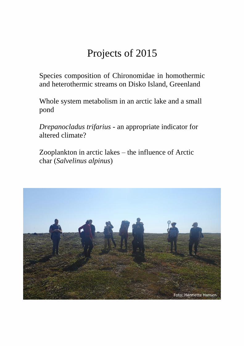
Projects of 2015
Species composition of Chironomidae in homothermic
and heterothermic streams on Disko Island, Greenland
Whole system metabolism in an arctic lake and a small
pond
Drepanocladus trifarius - an appropriate indicator for
altered climate?
Zooplankton in arctic lakes – the influence of Arctic
char (Salvelinus alpinus)
Foto: Henriette Hansen