Articol recenzie econometrie

8/12/2019 Articol recenzie econometrie

http://slidepdf.com/reader/full/articol-recenzie-econometrie 1/14

American Finance Association

The Constant Elasticity of Variance Model and Its Implications For Option PricingAuthor(s): Stan BeckersSource: The Journal of Finance, Vol. 35, No. 3 (Jun., 1980), pp. 661-673Published by: Blackwell Publishing for the American Finance AssociationStable URL: http://www.jstor.org/stable/2327490

Accessed: 19/10/2009 09:58

Your use of the JSTOR archive indicates your acceptance of JSTOR's Terms and Conditions of Use, available at

http://www.jstor.org/page/info/about/policies/terms.jsp. JSTOR's Terms and Conditions of Use provides, in part, that unless

you have obtained prior permission, you may not download an entire issue of a journal or multiple copies of articles, and you

may use content in the JSTOR archive only for your personal, non-commercial use.

Please contact the publisher regarding any further use of this work. Publisher contact information may be obtained at

http://www.jstor.org/action/showPublisher?publisherCode=black .

Each copy of any part of a JSTOR transmission must contain the same copyright notice that appears on the screen or printed

page of such transmission.

JSTOR is a not-for-profit service that helps scholars, researchers, and students discover, use, and build upon a wide range of content in a trusted digital archive. We use information technology and tools to increase productivity and facilitate new forms

of scholarship. For more information about JSTOR, please contact [email protected].

Blackwell Publishing and American Finance Association are collaborating with JSTOR to digitize, preserve

and extend access to The Journal of Finance.

http://www.jstor.org

http://www.jstor.org/stable/2327490?origin=JSTOR-pdf

http://www.jstor.org/page/info/about/policies/terms.jsp

http://www.jstor.org/action/showPublisher?publisherCode=black

http://www.jstor.org/action/showPublisher?publisherCode=black

http://www.jstor.org/page/info/about/policies/terms.jsp

http://www.jstor.org/stable/2327490?origin=JSTOR-pdf



THE JOURNAL OF FINANCE * VOL. XXXV, NO. 3 * JUNE 1980

The Constant Elasticity of Variance Model and Its

Implications For Option Pricing

STAN BECKERS*

I. Introduction

BLACK NDSCHOLES3] derived their seminal option pricingformula under theassumption that underlying stock price returns follow a lognormal diffusion

process:

S= 1 dt + a dZ

dSThis implies that the percentage price change, ?- , over the interval dt is normally

distributed with instantaneous mean, and instantaneous variance a2. While it is

well known that the lognormality assumption does not hold exactly, the pricing

of European call options has been studied recently for alternative diffusionmodels. Specifically, Cox [4] and Cox and Ross [5] focused their attention on the

constant elasticity of variance diffusion class:

dS = IS dt + uSa12 dZ (the elasticity factor0 c a < 2)

where the instantaneous variance of the percentage price change is equal toU2/S2- and hence is a direct inversefunctionof the stock price.In the tradition-ally used lognormal model, which corresponds to the limiting case a = 2, the

variance rate is not a function of the stock price itself. Both casual empiricismand economic rationale tend to supportthe inverserelationship.If this relation-ship is borne out by the empirical data, an option pricingformulabased on the

constant elasticity of variance diffusion could fit the actual marketprices betterthan the Black-Scholes model. In this article we empirically investigate therelationshipbetween the stock price level and its varianceof returnand performa comparativestatics analysisof the Black-Scholespricesand those based on twospecial cases of the constant elasticity of variance class (a = 1 and a = 0).

I. The Relationship Between the Variance of Stock Price Returns andthe Level of the Stock Price

It is sometimes argued that a simple economic mechanism might cause an inverserelationshipbetween the level of the stock price and its variance of return. If a

*VlaamseEkonomischeHogeschoolandEuropean nstitute forAdvancedStudies inManagement,Brussels. The author gratefully acknowledgesthe helpful suggestions of Mark Rubinstein, Barr

Rosenbeig and LarryJ. Merville.John Cox kindly providedus with a simplifiedformula for thesquareroot option price.All remainingerrorsare of course ours.

661



662 TheJournal of Finance

firm'sstock price falls, the market value of its equity tends to fall more rapidlythan the market value of its debt, causingthe debt-equityratio to rise;hence theriskiness of the stock increases.A similareffect could be observedeven if a firmhas almost no debt. Since every firm faces fixed costs, which have to be metirrespectiveof its income,a decreasein incomewill decreasethe value of the firmand at the same time increase its riskiness. Both operatingand financial everageargumentscan be used to explainthe inverserelationshipbetween varianceandstock price observed in the literature (Black [1], Schmalensee and Trippi [11]).Black [2] states that cause and effect also may be invertedso that a downturn nthe generalbusinessclimatemight lead to an increasein the stock price volatilityand hence to a dropin stock prices.

The Constant Elasticity of Variance (CEV) class of stock price distributionsestablishes a theoretical frameworkwithin which this inverserelationshipcan beempiricallytested. The instantaneousstandard deviationof the percentage pricechange for this class is given as aS(-2)/2 where0 'c a < 2. The standard deviationof the return distributionfluctuates inversely with the level of the stock price.This relationshipcan be restated as:

~ scvSt+dt\ (at- 2)(1In stdv

dtIn cr+ (a-2ln St(1

St ~~~2

If the CEV model wouldhold exactly, a simple regression

St+,In (stdvS =a+blnSt+wt (2)

St

could be used to check the magnitudeof the characteristicexponenta. However,several problemsarise in implementingthis procedureusing daily observations.

Although the relationship specified in (1) is instantaneous, equation (2) isexpressed over a finite time period. It can nevertheless be shown that a similarrelationshipalso holds over finite time. As a varies from2 to 0, the coefficient ofln St in (2) will decrease uniformly from 0 to -1. One can easily verify from

appendix A, for instance, that if a = 1, then

n (stdv S =ln k--In St where k = ((eT-1)-a2)/2.St ~~2

If the CEV model does not hold exactly, the regressionspecificationas given in(2)willbe incomplete. Althoughvarious economicfactors canimpactthe standarddeviation daily, it is practically impossibleto quantifythem on a daily basis andit is assumed that the stock markets are efficient enough to reflect these factors

via stock price changes.Since on any given day only one return observation is available, stdv (St+11St)

cannot be calculated exactly. The absolute value of In (St+, 1St) however, can be

used to operationalize the standard deviation if In St is normally distributed:

I n (St+, St) I s a realization of the underlyingdistribution with expected valueapproximatelyproportional o the standarddeviation (see appendix C). Since theCEV class of distributionsdiffersfrom the lognormalin scale only, the ratio of



Option Pricing 663

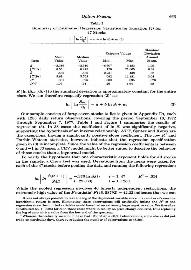
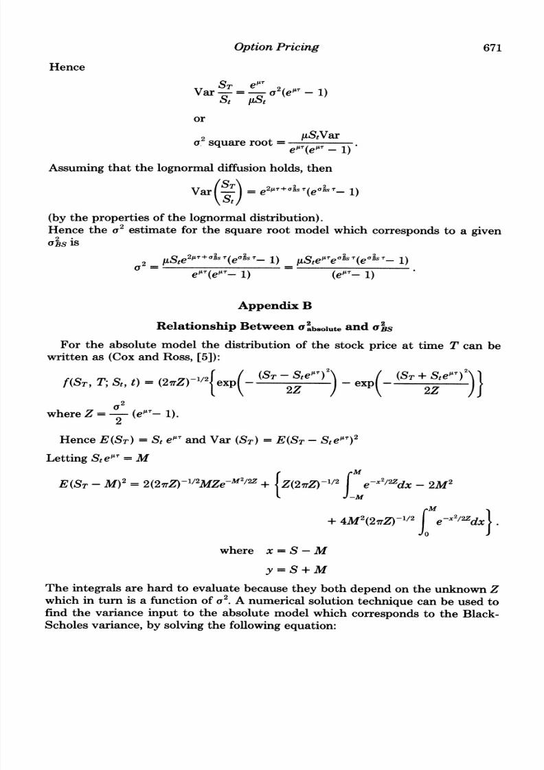
Table I

Summary of Estimated Regression Statistics for Equation (3) for

47 Stocks

In InS =a+bInSt+w(3)St

Standard

Extreme Values DeviationMean Median Around

Item Value Value Min. Max Mean.

a -2.389 -2.610 -6.607 3.483 1.99l T(d)l 8.55 8.975 .120 21.005 6.38

-.552 -.536 -2.231 .438 .52

l T(b) l 5.68 5.763 .092 11.481 3.04R2 .031 .026 .000 .095 .026DW 1.07 .94 .26 1.64 .38

E I n (St+,, St) Ito the standard deviation is approximately constant for the entire

class. We can therefore respecify regression (2)1 as:

St+1In in- =a+blnSt+wt (3)

St

Our sample consists of forty-seven stocks (a list is given in Appendix D), each

with 1253 daily return observations, covering the period September 18, 1972

through September 7, 1977. Table I and Figure 1 summarize the results of

regression (3). In 38 cases the coefficient of In St was significantly negative,

supporting the hypothesis of an inverse relationship. ATT, Syntex and Xerox are

the exceptions, having a significantly positive slope coefficient. The low R2 and

Durbin-Watson statistics, however, indicate that the regression specification

given in (3) is incomplete. Since the value of the regression coefficients is between

0 and -1 in 33 cases, a CEV model might be better suited to describe the behavior

of those stocks than a lognormal model.

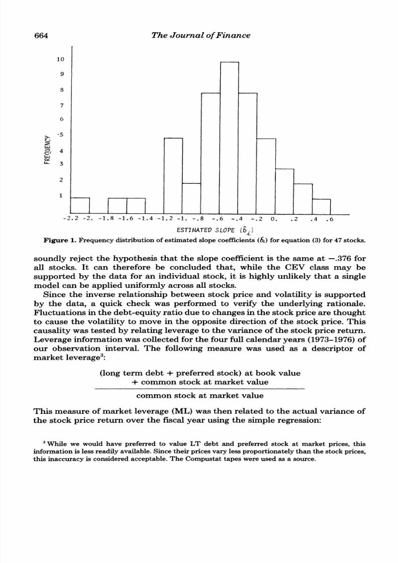
To verify the hypothesis that one characteristic exponent holds for all stocks

in the sample, a Chow test was used. Deviations from the mean were taken for

each of the 47 stocks before pooling the data and running the following regression:

In I1Si(t+ 1) -.3761nSi(t) i = 1, 47 R2 = .014

SA(t) (-29.369) t = 1, 1253

While the pooled regression involves 46 linearly independent restrictions, the

extremely high value of the F statistic2 F(46, 58792)=

42.22 indicates that we can1 t was not always possibleto take the log of the dependentvariablesince in a numberof cases the

logarithmic return is zero. Eliminating these observations will artificially inflate the R2 of theregression ince the omittedvariableswouldhave had an extremely argenegativevalue. Wethereforesubstituted(St+ .0625)forSt in those cases wherein realityno price change occurred, hus replacingthe log of zerowith a value fromthe low end of the spectrum.

2Whereastheoreticallywe should havehad 1253x 47 = 58,891observations, ome stocks did nottradeon particulardays, thereby reducing he numberof observations o 58,886.



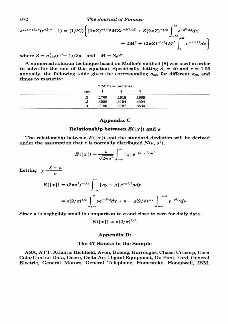
664 The Journal of Finance

10

9

8

7

6

~'

2

1

-2.2 -2. -1.8 -1.6 -1.4 -1.2 -1. -.8 -.6 -.4 -.2 0. .2 .4 .6

ESTIMATEDLOPE (bi.J

Figure 1. Frequencydistributionof estimatedslope coefficients(bi)forequation(3) for47 stocks.

soundly reject the hypothesis that the slope coefficient is the same at -.376 forall stocks. It can therefore be concluded that, while the CEV class may besupported by the data for an individualstock, it is highly unlikely that a singlemodel can be applieduniformlyacrossall stocks.

Since the inverse relationshipbetween stock price and volatility is supportedby the data, a quick check was performedto verify the underlyingrationale.Fluctuationsin the debt-equityratiodue to changesin the stockpricearethought

to cause the volatility to move in the opposite direction of the stock price. Thiscausalitywas tested by relatingleverageto the variance of the stock pricereturn.Leverageinformationwas collectedfor the fourfull calendaryears (1973-1976)ofour observation interval. The following measure was used as a descriptor ofmarketleverage3:

(long term debt + preferredstock) at book value+ common stock at marketvalue

common stock at marketvalue

This measure of marketleverage (ML)was then related to the actual variance of

the stock price returnover the fiscal year using the simple regression:

3While we would have preferredto value LT debt and preferredstock at market prices, thisinformation s less readilyavailable.Since theirpricesvaryless proportionatelyhan the stockprices,this inaccuracy s consideredacceptable.The Compustat apes were used as a source.



Option Pricing 665

(Vari(t) - Vari) = .143*10-4 (MLi(t) - ML) R2 = .045(2.967) DW = 2.17

To eliminate any differences n the level of responsebetweenstocks, all variableswere defined as deviations from their intertemporalmean. Although an increasein marketleveragedoes significantlyaffect the risk to the stockholders,a numberof other factorsapparentlyalso impactthis relationship.A moredetailedanalysisof the intertemporalbehavior of the variance would certainlybe warranted,butis beyond the scope of this paper.

Having empiricallyestablished the validity of using the CEVclass to describestock price behavior, it would be interesting to investigate the effect of thisalternative model specification on option pricing. Specifically, since the CEVclass might capture the actual stock price behavior better than the lognormalmodel, the correspondingoptionpricescouldgive a better fit to the actual optionmarket prices than the Black-Scholes model prices. The following section at-tempts to clarifythis questionusing a comparativestatics analysis.

H. A Comparative Statics Analysis

Cox [4] derived an option pricingformula which holds if the stock price followsa CEV diffusion. The derivation is based on an argumentfirst presentedby Coxand Ross [5]: if the return stream on a Europeancall option can be spanned bythe

underlyingstock and the risk-free

asset,then the

resulting differentialequation which governsthe call will hold for any set of investor preferences.Inparticular, a solution obtained under any specific assumption about investorpreferenceswill have complete generality.Assumingriskneutrality, the value ofan option is merely the expectedfuture value of the call at expirationdiscountedto the present at the risk-free rate. The solution to the option pricing problemthen depends on findingthe distributionof the stock price at expiration.Cox [4]foundthat if the stock pricefollowsthe CEVdiffusion, he continuouspartof thedensity of ST, conditional on St (t < T) is

f(ST, T; St, t) = (2 - a)kl/2-a(xyl-2a)l/2(l/2-a)eX_YIi/2-, (2(xy)l/2) (4)

where X = T-t

2A

a2(2 - a) (e9(2--),_j1)

x =kS2-ae (2-a)T

Y = kST

I, = modified Bessel function of the first kind of orderq.

The probability that ST = 0 is given by G , r) where G(m, v) is the

complimentary gamma distribution and r is the risk-free rate. This probabilityapproacheszero as a approaches2 (the lognormalcase).Giventhat the probabilitydistributionof STis known,Cox obtains the following option price:




C(S, ) = St>7 g(n + 1, x)G(n + 1 + -kK2a)

-Ker1 2 a'1x)G(n + 1, kK2a)

e-vrn-i

e vwhere g(m, v) = is the gammadensity function

r(m)

2r

=a2(2 -a)(er(2-a)T_ 1)

x = kS2-cer(2-a)T

K = striking price.

In our comparativestatics analysis we concentrateon two special cases of this

general formula:the squareroot model (a = 1) and the absolute model (a = 0).Cox and Ross [5] discuss both models as limiting cases of pure Markov jumpprocesses. In orderto comparethe Black-Scholes model and either of these two

models, we need to ensure that equivalent inputs are used in all models. Each ofthe three models under considerationdepends upon only five data inputs: the

stock price (S), time to maturity (T), the exercise price (K), the risk free rate (r)and an estimate of the stock price volatility (a2). We assume that Var(ST/St) isthe same for all the models compared n orderto ensure that consistentvolatilityestimates are used in the comparativestatics analysis. AppendicesA and B derive.the relationships between a2 square root and aJs and between a2 absolute and

2BSrespectively.Using these results we can proceedwith a comparativestatics analysis of the

three models. Note, however, that the option pricingformulafor the CEV class

contains an infinite summation which makes evaluation difficult in those cases

where convergenceis slow. This problemis easily solved for the absolute modelbecause Cox and Ross [5] introduce an alternative formulationfor the optionprice:

C(S, T) (S -Ke-rT )N(yi) + (S + Ke-rT)N(y2) + v(n(y1) - n(y2))

where N(*) = cumulativeunit normaldistributionfunction

n(*) = unit normal density function

v11 -(e-2rT 1/2

S - Ke-rTy1 =

V

-S - Ke-rT

Y2 =V



Option Pricing 667

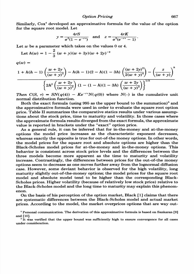
Similarly, Cox4 developed an approximative formula for the value of the option

for the squareroot model. Let

4rS 4rK

= a2(1 - e-rT) and z= 2(e-rT1)

Let w be a parameterwhich takes on the values 0 or 4.

Let h(w) = 1 - - (w + y)(w + 3y)(w + 2y)23

q(w) =

(w +2y ((w+ 2y)2\h

1 + h(h- 1) (( - h(h- 1)(2 - h)(1 - 3h) 2(+y)4)-

w +~~2y 1/2{2h2 ((W y2) (1- (1- h)(1 - 3h) w

(W + Y)2 ~~~(Wy)2

Then C(S, T) = SN(q(4)) - Ke-rTN(q(O)) where N(.) is the cumulative unit

normaldistributionfunction.Both the exact formula(using995as the upperboundto the summation)5and

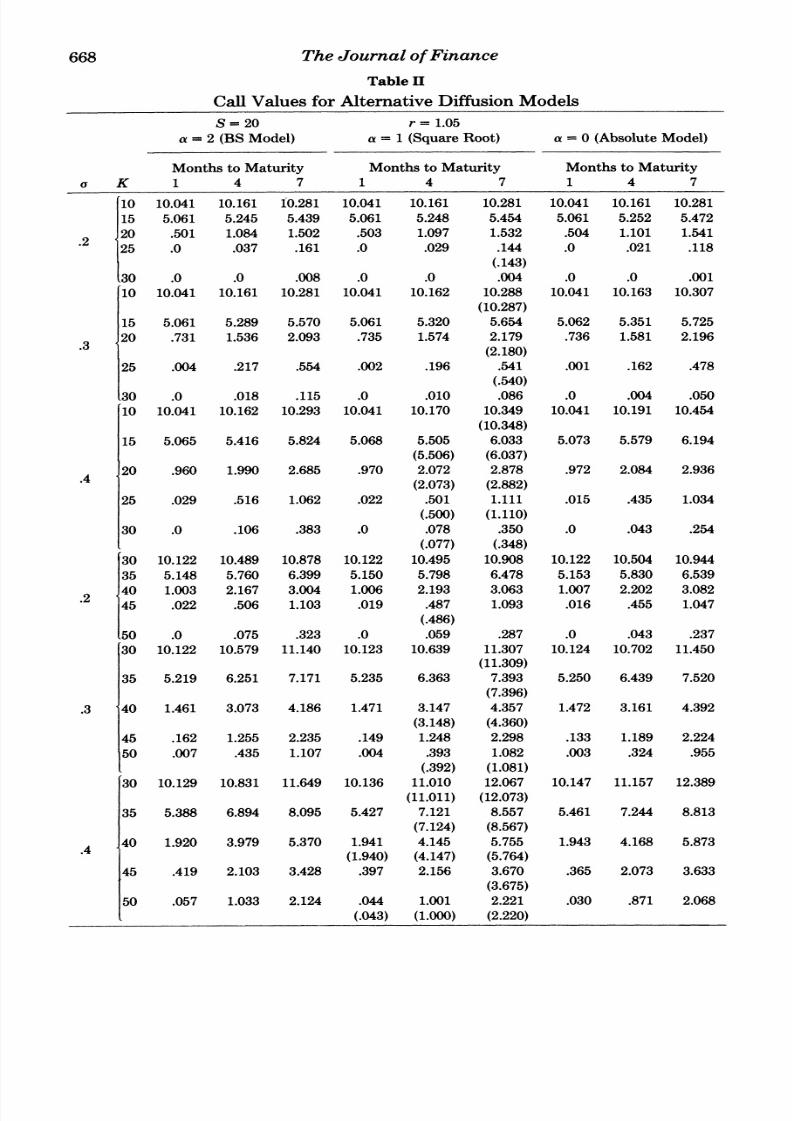
the approximative ormulawere used in order to evaluate the squareroot optionprice.Table II summarizes he comparativestatics results undervariousassump-

tions about the stock price, time to maturityand volatility. In those cases wherethe approximate ormularesultsdiverged rom the exactformula, he approximatevalue is reportedin bracketsunderthe exact option price.

As a general rule, it can be inferred that for in-the-money and at-the-money

options the model price increases as the characteristic exponent decreases,whereasexactly the opposite is true forout-of-themoney options.In otherwords,the model prices for the square root and absolute options are higher than the

Black-Scholes model prices for at-the-money and in-the-money options. This

behavior is consistent across stock price levels and the differencesbetween the

three models become more apparent as the time to maturity and volatilityincrease. Contrastingly, he differencesbetween prices for the out-of-the moneyoptions seem to decreaseas one moves furtherawayfromthe lognormaldiffusioncase. However, some deviant behavior is observed for the high volatility, longmaturity slightly out-of-the-money options;the model prices for the squarerootmodel and absolute model tend to be higher than the correspondingBlack-

Scholes prices.Higher volatility (becauseof relativelylow stock price)relative to

the Black-Scholesmodel and the long time to maturity may explainthis phenom-enon.

Onthe basisof his

perceptionof the

optionmarket,Black

[1]claims that there

are systematic differencesbetween the Black-Scholes model and actual market

prices. Accordingto the model, the market overprices options that are way out-

'Personal communication.The derivationof this approximativeormula s based on Sankaran 9]

and [10].5It was verifiedthat the upper bound was sufficientlyhigh to ensure convergencefor all cases

underconsideration.



668 TheJournal of Finance

Table II

CallValues for AlternativeDiffusionModels

S= 20 r= 1.05

a = 2 (BS Model) a = 1 (Square Root) a = 0 (Absolute Model)

Months to Maturity Months to Maturity Months to Maturity

a K 1 4 7 1 4 7 1 4 7

10 10.041 10.161 10.281 10.041 10.161 10.281 10.041 10.161 10.281

15 5.061 5.245 5.439 5.061 5.248 5.454 5.061 5.252 5.472

20 .501 1.084 1.502 .503 1.097 1.532 .504 1.101 1.541

25 .0 .037 .161 .0 .029 .144 .0 .021 .118

(.143)

30 .0 .0 .008 .0 .0 .004 .0 .0 .001

10 10.041 10.161 10.281 10.041 10.162 10.288 10.041 10.163 10.307

(10.287)

15 5.061 5.289 5.570 5.061 5.320 5.654 5.062 5.351 5.72520 .731 1.536 2.093 .735 1.574 2.179 .736 1.581 2.196

(2.180)

25 .004 .217 .554 .002 .196 .541 .001 .162 .478

(.540)

30 .0 .018 .115 .0 .010 .086 .0 .004 .050

10 10.041 10.162 10.293 10.041 10.170 10.349 10.041 10.191 10.454

(10.348)

15 5.065 5.416 5.824 5.068 5.505 6.033 5.073 5.579 6.194

(5.506) (6.037)

20 .960 1.990 2.685 .970 2.072 2.878 .972 2.084 2.936

(2.073) (2.882)25 .029 .516 1.062 .022 .501 1.111 .015 .435 1.034

(.500) (1.110)

30 .0 .106 .383 .0 .078 .350 .0 .043 .254

(.077) (.348)

30 10.122 10.489 10.878 10.122 10.495 10.908 10.122 10.504 10.944

35 5.148 5.760 6.399 5.150 5.798 6.478 5.153 5.830 6.539

2 40 1.003 2.167 3.004 1.006 2.193 3.063 1.007 2.202 3.082

45 .022 .506 1.103 .019 .487 1.093 .016 .455 1.047

(.486)

50 .0 .075 .323 .0 .059 .287 .0 .043 .237

30 10.122 10.579 11.140 10.123 10.639 11.307 10.124 10.702 11.450(11.309)

35 5.219 6.251 7.171 5.235 6.363 7.393 5.250 6.439 7.520

(7.396)

.3 40 1.461 3.073 4.186 1.471 3.147 4.357 1.472 3.161 4.392

(3.148) (4.360)

45 .162 1.255 2.235 .149 1.248 2.298 .133 1.189 2.224

50 .007 .435 1.107 .004 .393 1.082 .003 .324 .955

(.392) (1.081)

30 10.129 10.831 11.649 10.136 11.010 12.067 10.147 11.157 12.389

(11.011) (12.073)

35 5.388 6.894 8.095 5.427 7.121 8.557 5.461 7.244 8.813

(7.124) (8.567)

40 1.920 3.979 5.370 1.941 4.145 5.755 1.943 4.168 5.873

.4 (1.940) (4.147) (5.764)

45 .419 2.103 3.428 .397 2.156 3.670 .365 2.073 3.633

(3.675)

50 .057 1.033 2.124 .044 1.001 2.221 .030 .871 2.068

(.043) (1.000) (2.220)



Option Pricing 669

Table 11-Continued

S= 20 r= 1.05a = 2 (BS Model) a = 1 (Square Root) a = 0 (Absolute Model)

Months to Maturity Months to Maturity Months to Maturitya K 1 4 7 1 4 7 1 4 7

50 10.203 10.916 11.718 10.204 10.954 11.816 10.205 10.992 11.902

(11.817)

55 5.304 6.554 7.665 5.314 6.619 7.789 5.324 6.669 7.872

.2 1 (7.790)

60 1.504 3.251 4.506 1.509 3.290 4.595 1.511 3.302 4.623

65 .158 1.302 2.373 .149 1.287 2.390 .138 1.250 2.347

70 .005 .421 1.125 .004 .387 1.087 .003 .341 1.005

(.386) (1.086)

50 10.229 11.394 12.596 10.241 11.545 12.918 10.253 11.664 13.131

(11.546) (12.922)

55 5.597 7.559 9.086 5.631 7.724 9.411 5.659 7.818 9.565

(7.725) (9.415)

60 2.192 4.609 6.279 2.206 4.721 6.536 2.209 4.742 6.588

(4.722) (6.540)

65 .565 2.587 4.170 .545 2.615 4.320 .519 2.554 4.259

(4.322)

70 .094 1.345 2.673 .079 1.307 2.715 .064 1.202 2.566

(1.306)

50 10.345 12.157 13.785 10.387 12.490 14.477 10.428 12.702 14.910

(12.494) (14.491)55 6.034 8.702 10.641 6.099 9.028 11.313 6.147 9.172 11.636

(9.032) (11.328)

60 2.880 5.969 8.055 2.911 6.217 8.633 2.915 6.252 8.809

.4 (6.220) (8.646)

65 1.102 3.936 5.995 1.082 4.073 6.434 1.040 3.994 6.452

(4.074) (6.443)

70 .340 2.507 4.397 .306 2.536 4.684 .263 2.375 4.560

(2.535) (4.687)

of-the-moneyandunderpricesoptionsthat areway into-the-money.Optionswithless than three months to maturity also tend to be underpriced.Under thesecircumstances, he squareroot and absolute modelshold little promisesince theytend to worsenthe fit to the marketprices ratherthan improve it.

However, a recent study by MacBeth and Merville [7] arguesthat the devia-tions between market prices and Black-Scholesmodel prices counterposethoseobserved by Black. For a limited sample (6 options) studied over the 1976calendaryear,they findthat the model understates(overstates)the marketpricesfor deep into (out of) the money options.Althoughtheir conclusionscan only be

consideredtentative becauseof the limited sample,it appearsthat the CEV classmight have been better suited to describethe behavior of those options in 1976.It is obvious that futher extensive study is needed to conclusively establish

the deviationbetween Black-Scholes and marketprices.If the MacBeth-Merville

findings are confirmed,the CEV class of option pricingshould be considered as

a primne lternative formulation. In that case it will also be comfortingto know

that, as can be inferredfromTable 2, the simplifiedformulasuggestedby Coxfor




the square root model can readily be used as a substitute for the general

formulation.

III. Conclusion

On the basis of the empirical study performed,it appears that the constant

elasticity of varianceclass could be a better descriptorof the actual stock price

behavior than the traditionallyused lognormalmodel. While no generalmodel

apparently applies for all stocks, most of the stocks analyzed in this paper

exhibited a significantnegative relationshipbetween the level of the stock price

and its volatility. Some evidence also exists that part of this relationshipcan be

attributedto changes in the debt-equityratio causedby fluctuationsin the stock

price.On the basis of this limited evidence,a model based on the simplevariancenonstationarity inherent in the constant elasticity of variance class might be

preferableto the traditionallyused lognormalmodel.The comparativestatics analysisof the Black-Scholes,squarerootand absolute

models indicatesthat their pricesdiffersystematically.The constantelasticity of

varianceclass yields priceswhich are higherthan the Black-Scholespricesfor in-

the-money and at-the-money options, while the reverse is true for out-of-the-

money options. Some recent empiricalevidence suggests that these are exactly

the deviations being observed in practice between the Black-Scholesprice pre-

dictionsand marketprices.If these results hold true for an extensive sample,theconstant elasticity of variance class could become a prime alternative model

specificationto the canonicalBlack-Scholesformula.

Appendix A

For the squareroot model the distributionof ST can be written as

f(ST, T) = k(x/y)l/2ex-YI(2(xy)l/2) from (4) where a = 1

orf(ST T) =kx - o e(x__ fi n+1(y) (by Feller [6], p. 58)

n=0O(n +1)

where

1 v1 -axfa,v(X) ax e

G(v)

is the gamma density finction.

As y = kST,

f()=Xn=O (n + ) i+()

The moments of f( y) are equal to

e-xxn

E(yJ) = x> (n ) (n+j)(n+j-1)...(n+ 1).



Option Pricing 671

Hence

ST el 2 AVar = -(e 1)SSt

or

2 ,uStVara, square root =

e/T(e T- 1)

Assuming that the lognormal diffusionholds, then

Var (S) e S(eB 1)

(by the propertiesof the lognormaldistribution).Hence the a2 estimate for the square root model which correspondsto a givenUBS is

,Ste2'/T+ 'YBsT(eBS T_

1) ,uSte /AeBS

T(eOBST-

l )=- =

e/AT(e/T_ 1) (e IT_1)

Appendix B

Relationship Between absolute and 4BS

For the absolute model the distribution of the stock price at time T can bewritten as (Coxand Ross, [5]):

(2Z1/2Jex (ST- Ste ) (2 (ST St'T2f(ST, T; St, t) = (2I-TZ) exp-- exp

a2 ~~~~~~~2Z2Z)where Z =- (eI- 1).

2

Hence E(ST) = St ey and Var (ST) = E(ST - Ste )2

Letting Ste'T = M

E(ST - M)2 = 2(2STZ)-1/2MZe-M2/2Z Z(27TZ)-1/2 e-x22zdx 2M2

+ 4M2(2TZ-1/2 A x2/2zddx

where x =S-M

y=S+M

The integrals are hard to evaluate because they both depend on the unknown Z

which in turn is a function of a2. A numerical solution technique can be used to

find the variance input to the absolute model which corresponds to the Black-

Scholes variance, by solving the following equation:




e2+

BS T(eFBS 1) = (1/S2).{ (2Z) 1/22MZeM2/2 + Z(2 1/Z) 2 e zx2/2zdx

-2M2 + (21TZ)-1/24M2 1M ex2/2zdx}

where Z = aabs(e -1)/2,u and M = Ste

A numericalsolutiontechniquebasedon Muller'smethod [8] was used in orderto solve for the root of this equation. Specifically,letting St = 40 and r = 1.05annually, the following table gives the correspondingCabs for different aBS and

times to maturity:

TMT (in months)

GBS 1 4 7

.2 .1769 .1818 .1868

.3 .4006 .4194 .4394

.4 .7185 .7727 .8504

Appendix C

Relationship between E( I j) and a

The relationship between E( Ix I)and the standarddeviation will be derivedunder the assumptionthat x is normallydistributedN(,u,a2).

E(lxf) = Ie

Letting y _X-fi

E(IxI) = (2mT(2)-1/2

cay + I I e-Y2/2 ady

= a(2/v)1/2 ye-Y2/2dy + fi - u(2/iT)1/2 -Y2/2dy

Since , is negligiblysmall in comparison o a and close to zero for daily data.

E ( x }) _- c(2/vo)1

Appendix D:

The 47 Stocks in the Sample

ASA, ATT, AtlanticRichfield, Avon,Boeing,Burroughs,Chase, Citicorp,CocaCola;ControlData, Deere, Delta Air, Digital Equipment,Du Pont, Ford,GeneralElectric, General Motors, General Telephone, Homestake, Honeywell, IBM,



Option Pricing 673

International Minerals, ITT, Kennecott, Loews, McDonalds, Merrill Lynch,Monsanto,National Semiconductor,NorthwestAir, Occidental,Pfizer, Polaroid,RCA, Schlumberger,Searle, Sears, Skyline, Sperry,Syntex, Texas Instruments,

Tiger, U.S. Steel, Upjohn, WesternUnion, Westinghouse,and Xerox.

REFERENCES

1. F. Black. FactandFantasy n the Use of Options. Financial AnalystsJournal 31 (July-August1975).

2. F. Black. Studies of Stock Price Volatility Changes. Proceedings of the 1976Meetings of theAmericanStatisticalAssociation,Businessand EconomicStatistics Division.

3. F. Black and M. Scholes. The Pricingof Optionsand OtherCorporateLiabilities. Journal of

Political Economy81 (May-June 1973):4. J. Cox. Notes on Option PricingI: ConstantElasticityof VarianceDiffusions. WorkingPaper

StanfordUniversity, September 1975).5. J. Cox and S. Ross. TheValuationof Options orAlternativeStochasticProcesses. Journal of

Financial Economics 3 (Jan-March1976).6. W. Feller.An Introductionto Probability Theoryand its Applications.Vol.2, 2d ed. (New York:

J. Wileyand Sons, 1971).7. J. MacBeth and L. Merville. AnEmpiricalExaminationof the Black-ScholesCallOptionPricing

Model Journal of Finance 34 (December1979).8. D. E. Muller. A Method for Solving Algebraic Equations Using an Automatic Computer.

Mathematical Tables and OtherAids to Computation10 (Spring 1956).9. M. Sankaran. Onthe Non-CentralChi-SquareDistribution. Biometrika 46 (July 1959).

10. . Approximationso the Non-CentralChi-SquareDistribution. Biometrika 50 (August1963).

11. R. Schmalensee and R. R. Trippi. CommonStock Volatility Expectations Impliedby OptionPremia. Journal of Finance 33 (March1978).

Documents

Articol recenzie econometrie