Embed Size (px)
Citation preview
8/3/2019 Aspen Radfrac
http://slidepdf.com/reader/full/aspen-radfrac 1/35
RadFrac for Dummies:
A How to Guide on Aspen Plus
This example will show how to use Radfrac on Aspen Plus to model distillationcolumns. The feed shown in the diagram above will consist of 50 lbmol/hr ofMethanol and 50 lbmol/hr of water. A purity of 99.5% is desired in both thebottoms and distillate product streams using a reflux ratio of 1.5.
DISTFEED
DISTILL
BOTTOMS
8/3/2019 Aspen Radfrac
http://slidepdf.com/reader/full/aspen-radfrac 2/35
Radfrac © SDSM&T 2/35
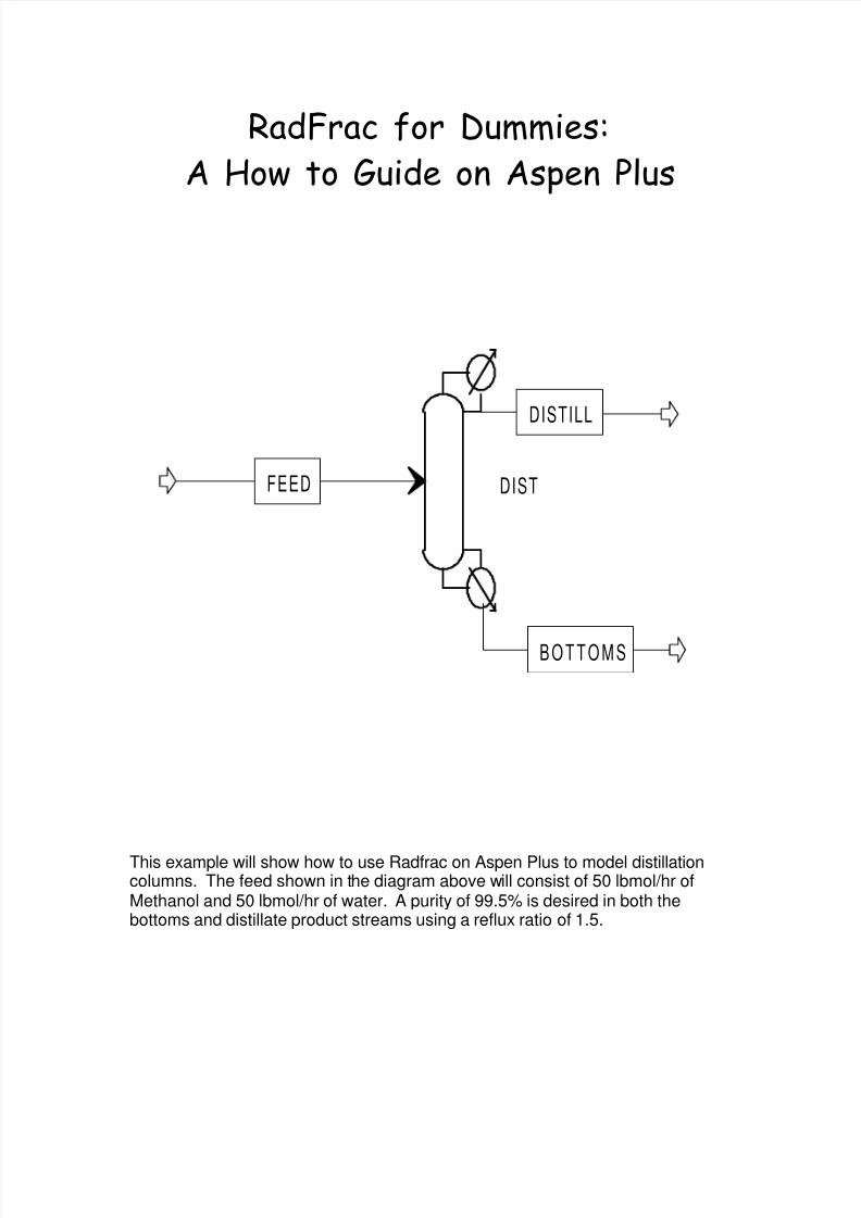
If you don’t know how to log on toAspen Plus, please see the
“Getting Started on Aspen Plus”manual.
Choose the Template Option
Click “OK.”
This window allows you
to select a particularsimulation option. For
this example, select the“General with EnglishUnits” option. Also, make
sure that the option in theRun Type box displays“Flowsheet”
Click “OK”
8/3/2019 Aspen Radfrac
http://slidepdf.com/reader/full/aspen-radfrac 3/35
Radfrac © SDSM&T 3/35
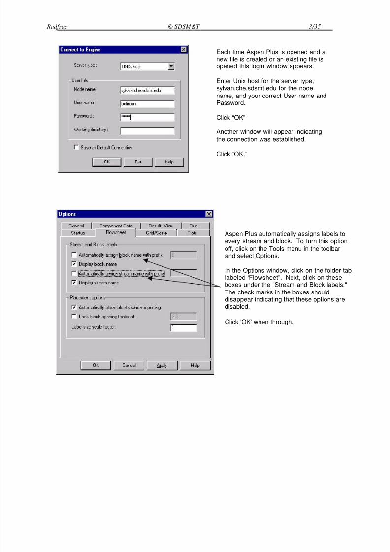
Each time Aspen Plus is opened and anew file is created or an existing file isopened this login window appears.
Enter Unix host for the server type,sylvan.che.sdsmt.edu for the node
name, and your correct User name andPassword.
Click “OK”
Another window will appear indicating
the connection was established.
Click “OK.”
Aspen Plus automatically assigns labels toevery stream and block. To turn this option
off, click on the Tools menu in the toolbarand select Options.
In the Options window, click on the folder tablabeled “Flowsheet”. Next, click on theseboxes under the "Stream and Block labels."
The check marks in the boxes shoulddisappear indicating that these options aredisabled.
Click 'OK' when through.
8/3/2019 Aspen Radfrac
http://slidepdf.com/reader/full/aspen-radfrac 4/35
Radfrac © SDSM&T 4/35
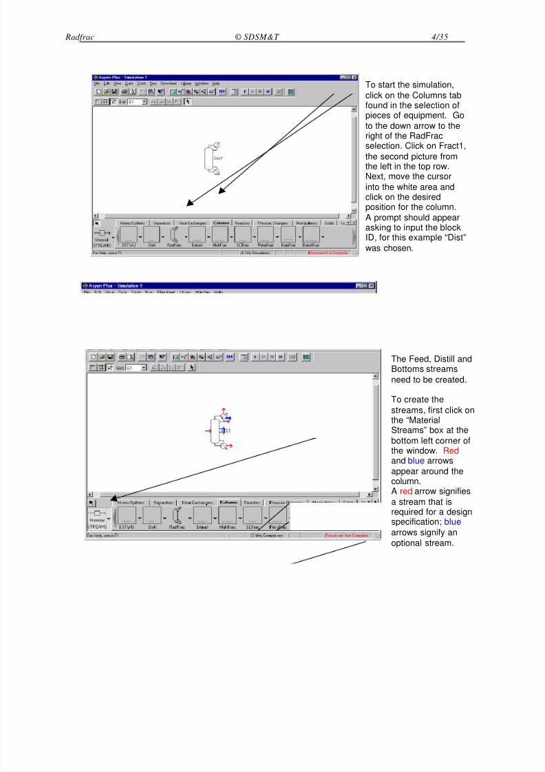
To start the simulation,
click on the Columns tabfound in the selection ofpieces of equipment. Go
to the down arrow to the
right of the RadFracselection. Click on Fract1,
the second picture fromthe left in the top row.Next, move the cursor
into the white area andclick on the desiredposition for the column.
A prompt should appearasking to input the blockID, for this example “Dist”
was chosen.
The Feed, Distill andBottoms streams
need to be created.
To create the
streams, first click onthe “MaterialStreams” box at the
bottom left corner ofthe window. Redand blue arrows
appear around thecolumn.A red arrow signifies
a stream that isrequired for a designspecification; blue
arrows signify an
optional stream.
8/3/2019 Aspen Radfrac
http://slidepdf.com/reader/full/aspen-radfrac 5/35
Radfrac © SDSM&T 5/35
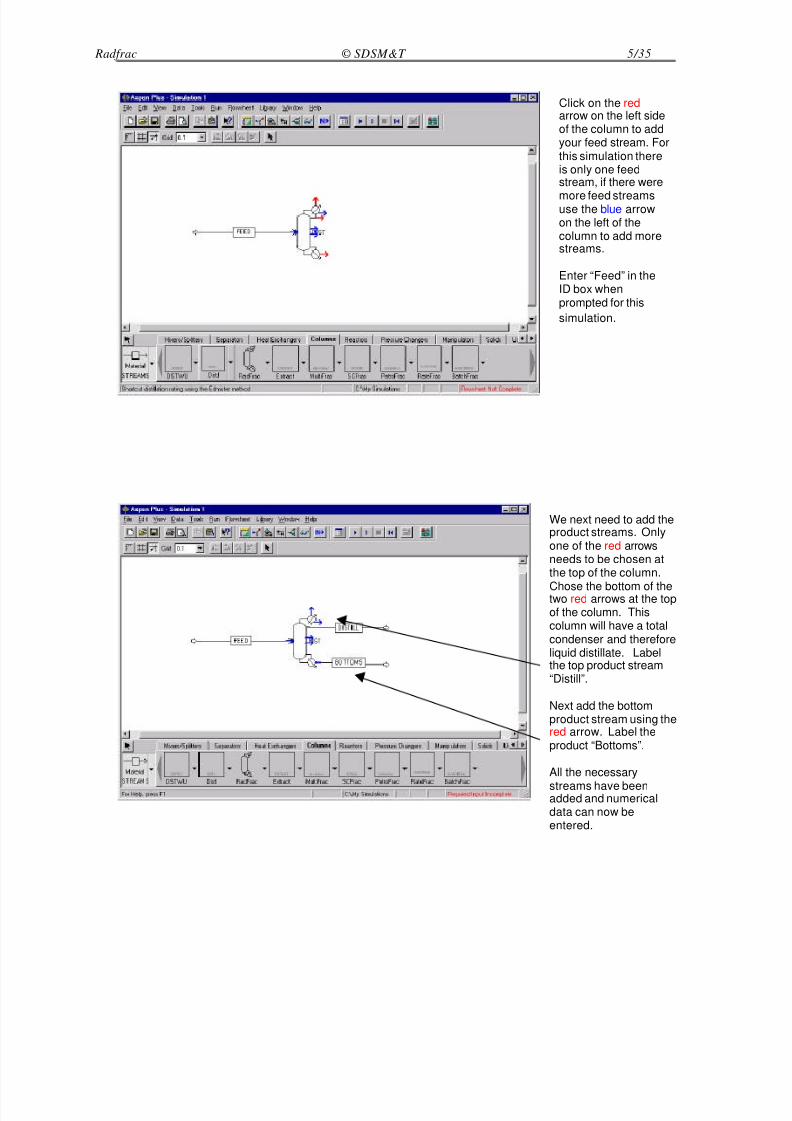
Click on the redarrow on the left sideof the column to addyour feed stream. Forthis simulation thereis only one feedstream, if there were
more feed streamsuse the blue arrowon the left of thecolumn to add morestreams.
Enter “Feed” in theID box whenprompted for this
simulation.
We next need to add theproduct streams. Onlyone of the red arrowsneeds to be chosen atthe top of the column.
Chose the bottom of thetwo red arrows at the topof the column. Thiscolumn will have a totalcondenser and thereforeliquid distillate. Labelthe top product stream“Distill”.
Next add the bottomproduct stream using thered arrow. Label theproduct “Bottoms”.
All the necessary
streams have beenadded and numericaldata can now beentered.
8/3/2019 Aspen Radfrac
http://slidepdf.com/reader/full/aspen-radfrac 6/35
Radfrac © SDSM&T 6/35
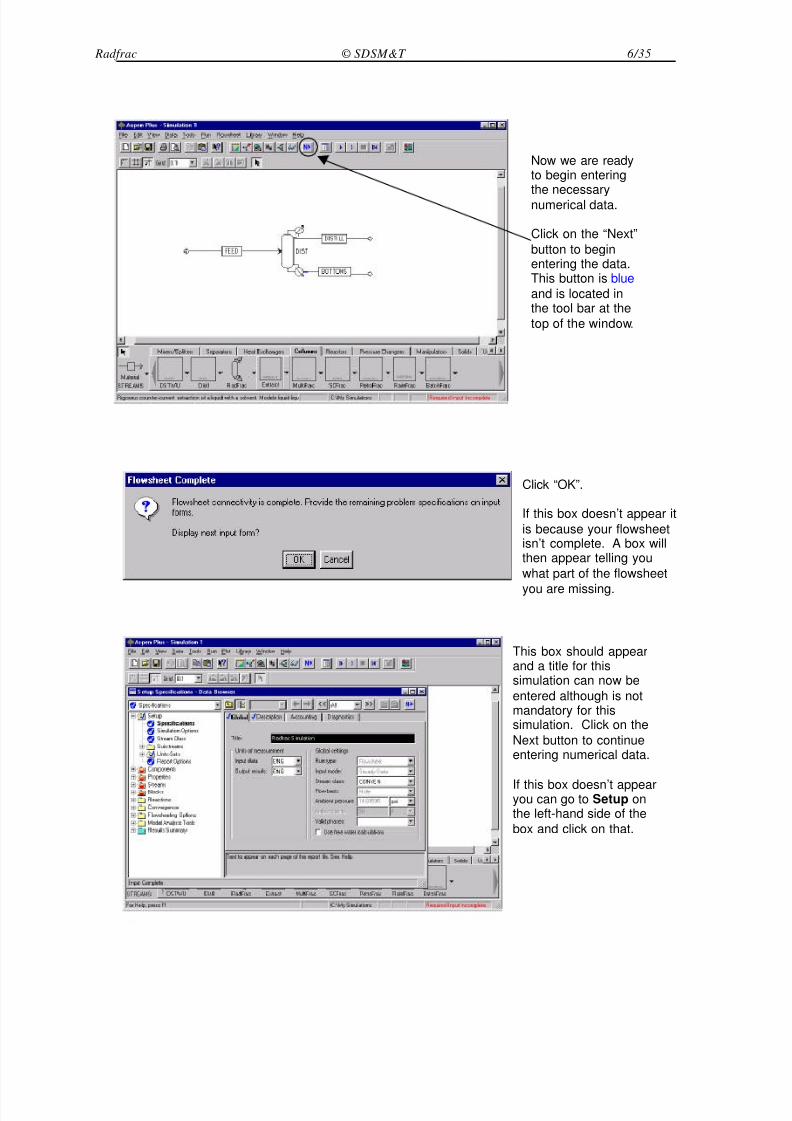
Now we are readyto begin entering
the necessarynumerical data.
Click on the “Next”
button to beginentering the data.This button is blue
and is located inthe tool bar at the
top of the window.
Click “OK”.
If this box doesn’t appear it
is because your flowsheetisn’t complete. A box willthen appear telling you
what part of the flowsheet
you are missing.
This box should appearand a title for thissimulation can now be
entered although is notmandatory for thissimulation. Click on the
Next button to continueentering numerical data.
If this box doesn’t appearyou can go to Setup onthe left-hand side of the
box and click on that.
8/3/2019 Aspen Radfrac
http://slidepdf.com/reader/full/aspen-radfrac 7/35
Radfrac © SDSM&T 7/35
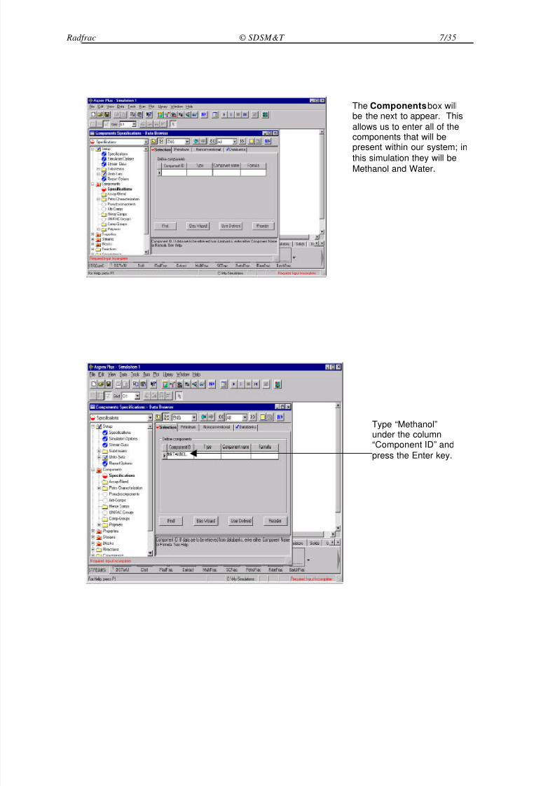
The Components box willbe the next to appear. This
allows us to enter all of the
components that will bepresent within our system; in
this simulation they will be
Methanol and Water.
Type “Methanol”under the column“Component ID” and
press the Enter key.
8/3/2019 Aspen Radfrac
http://slidepdf.com/reader/full/aspen-radfrac 8/35
Radfrac © SDSM&T 8/35
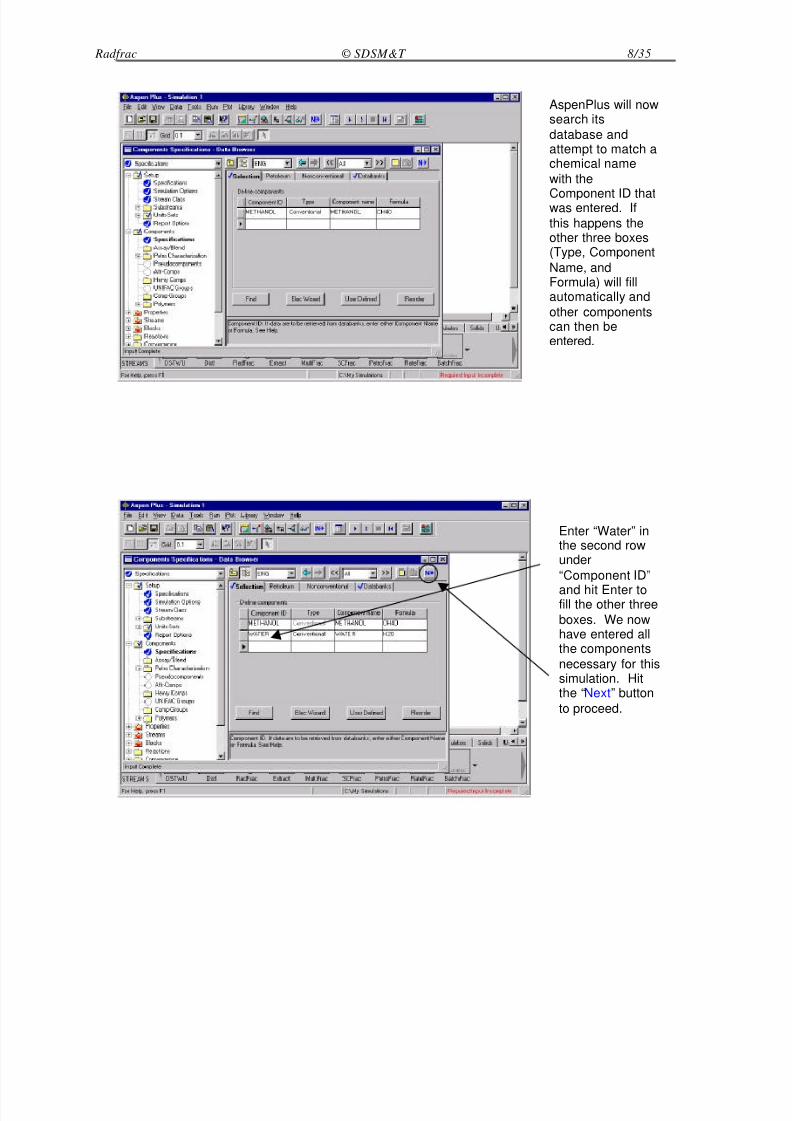
AspenPlus will nowsearch its
database andattempt to match achemical name
with the
Component ID thatwas entered. If
this happens theother three boxes(Type, Component
Name, andFormula) will fillautomatically and
other componentscan then beentered.
Enter “Water” inthe second rowunder
“Component ID”
and hit Enter tofill the other three
boxes. We nowhave entered allthe components
necessary for thissimulation. Hitthe “Next” button
to proceed.
8/3/2019 Aspen Radfrac
http://slidepdf.com/reader/full/aspen-radfrac 9/35
Radfrac © SDSM&T 9/35
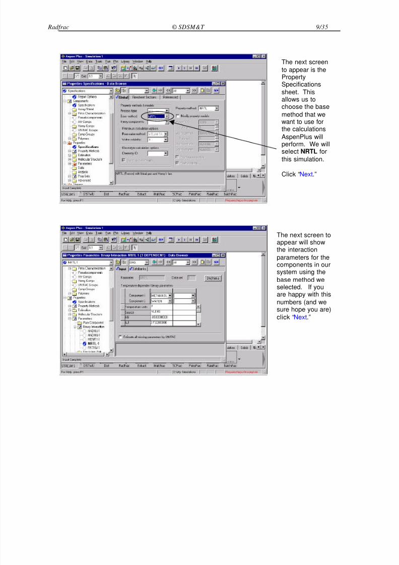
The next screen
to appear is thePropertySpecifications
sheet. This
allows us tochoose the base
method that wewant to use forthe calculations
AspenPlus willperform. We willselect NRTL for
this simulation.
Click “Next.”
The next screen toappear will showthe interaction
parameters for thecomponents in oursystem using the
base method weselected. If you
are happy with thisnumbers (and wesure hope you are)
click “Next.”
8/3/2019 Aspen Radfrac
http://slidepdf.com/reader/full/aspen-radfrac 10/35
Radfrac © SDSM&T 10/35
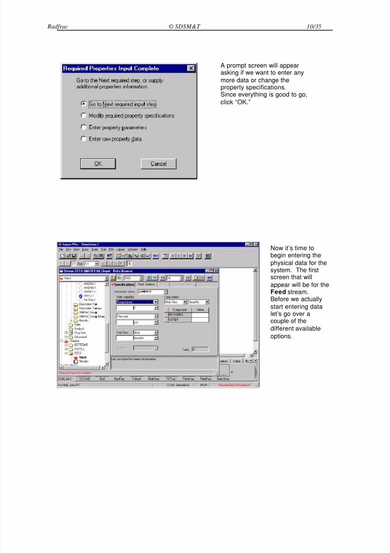
A prompt screen will appearasking if we want to enter any
more data or change theproperty specifications.
Since everything is good to go,click “OK.”
Now it’s time tobegin entering the
physical data for thesystem. The firstscreen that will
appear will be for the
Feed stream.Before we actually
start entering datalet’s go over acouple of the
different available
options.
8/3/2019 Aspen Radfrac
http://slidepdf.com/reader/full/aspen-radfrac 11/35
Radfrac © SDSM&T 11/35
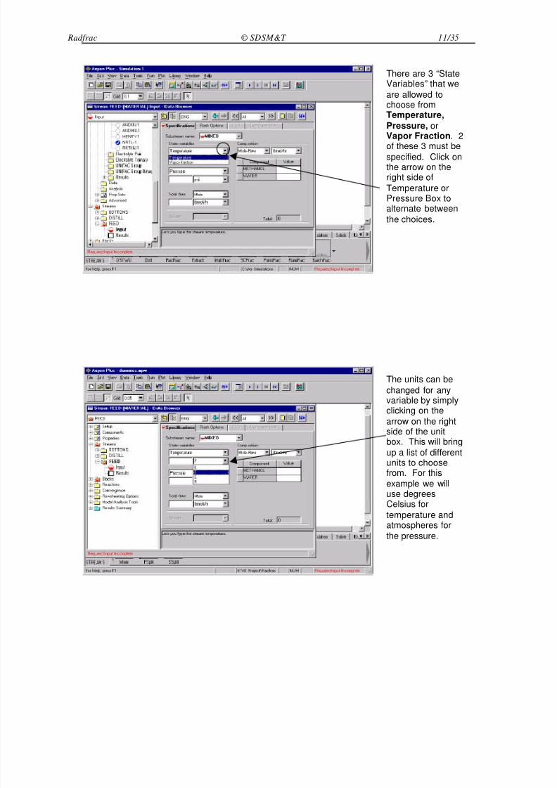
There are 3 “StateVariables” that we
are allowed tochoose fromTemperature,
Pressure, or
Vapor Fraction. 2of these 3 must be
specified. Click onthe arrow on theright side of
Temperature orPressure Box toalternate between
the choices.
The units can be
changed for anyvariable by simply
clicking on thearrow on the rightside of the unitbox. This will bring
up a list of differentunits to choosefrom. For this
example we willuse degreesCelsius for
temperature andatmospheres for
the pressure.
8/3/2019 Aspen Radfrac
http://slidepdf.com/reader/full/aspen-radfrac 12/35
Radfrac © SDSM&T 12/35
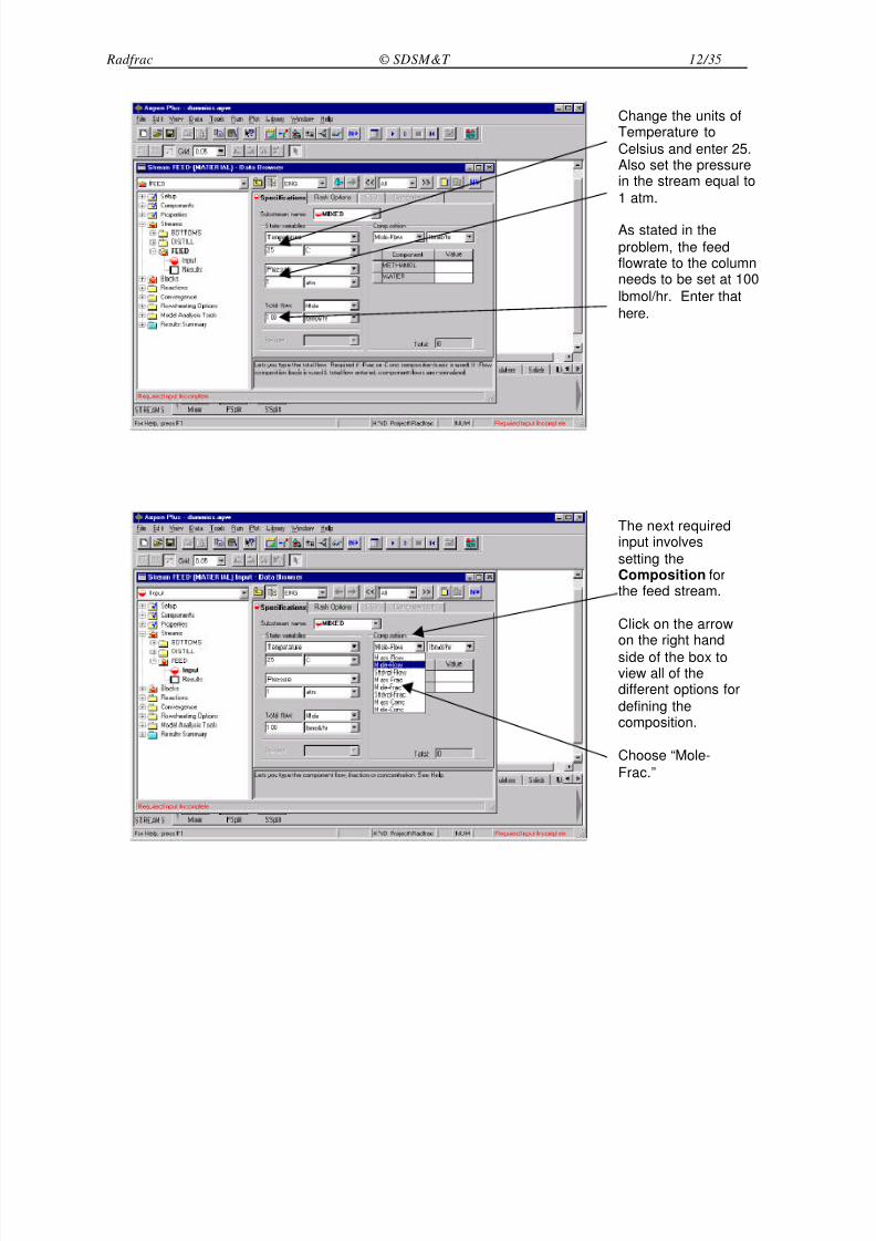
Change the units ofTemperature to
Celsius and enter 25.Also set the pressurein the stream equal to
1 atm.
As stated in the
problem, the feedflowrate to the columnneeds to be set at 100
lbmol/hr. Enter that
here.
The next requiredinput involves
setting theComposition forthe feed stream.
Click on the arrowon the right hand
side of the box toview all of thedifferent options for
defining thecomposition.
Choose “Mole-
Frac.”
8/3/2019 Aspen Radfrac
http://slidepdf.com/reader/full/aspen-radfrac 13/35
Radfrac © SDSM&T 13/35
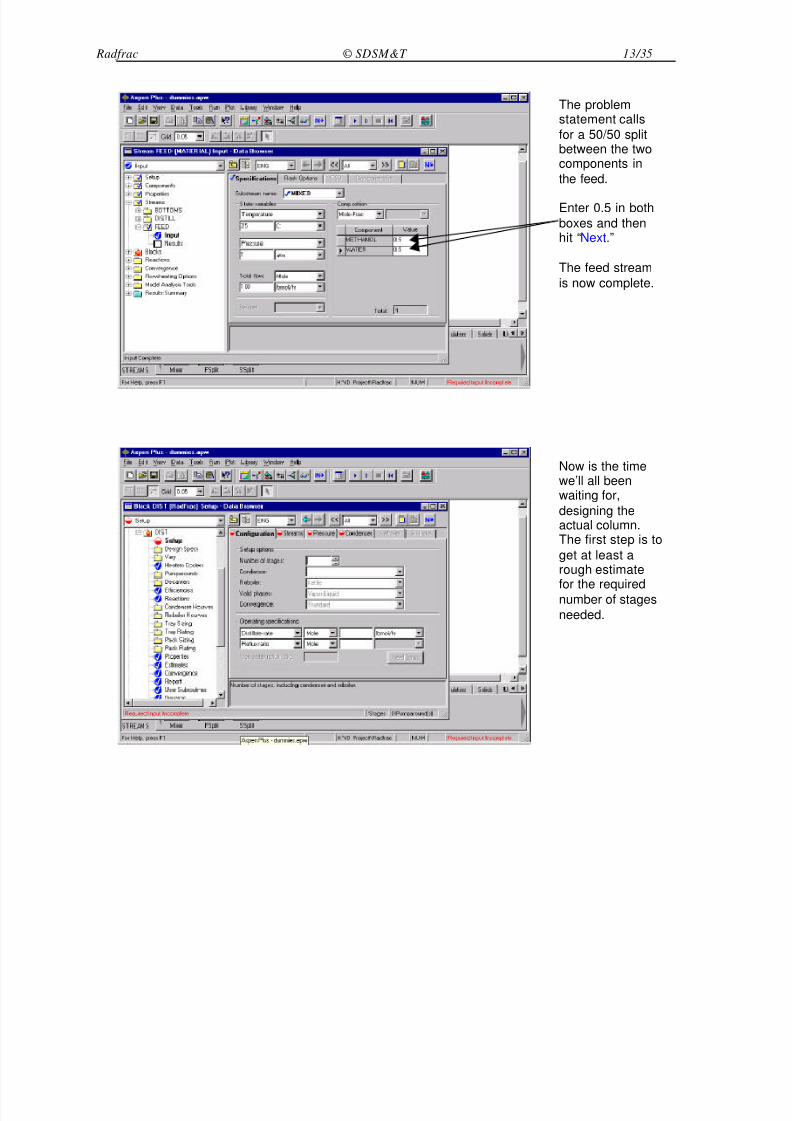
The problemstatement calls
for a 50/50 splitbetween the twocomponents in
the feed.
Enter 0.5 in both
boxes and thenhit “Next.”
The feed stream
is now complete.
Now is the timewe’ll all beenwaiting for,
designing theactual column.The first step is to
get at least arough estimate
for the requirednumber of stages
needed.
8/3/2019 Aspen Radfrac
http://slidepdf.com/reader/full/aspen-radfrac 14/35
Radfrac © SDSM&T 14/35
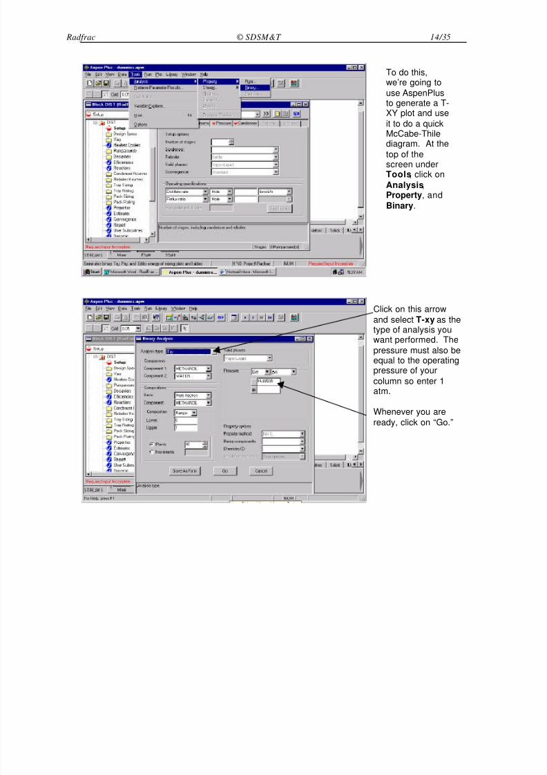
To do this,we’re going to
use AspenPlusto generate a T-XY plot and use
it to do a quick
McCabe-Thilediagram. At the
top of thescreen underTools, click on
Analysis,Property, and
Binary.
Click on this arrow
and select T-xy as thetype of analysis youwant performed. The
pressure must also beequal to the operatingpressure of your
column so enter 1atm.
Whenever you are
ready, click on “Go.”
8/3/2019 Aspen Radfrac
http://slidepdf.com/reader/full/aspen-radfrac 15/35
Radfrac © SDSM&T 15/35
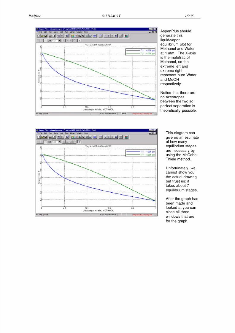
AspenPlus shouldgenerate this
liquid/vaporequilibrium plot forMethanol and Water
at 1 atm. The X-axis
is the molefrac ofMethanol, so the
extreme left andextreme rightrepresent pure Water
and MeOHrespectively.
Notice that there areno azeotropesbetween the two so
perfect separation is
theoretically possible.
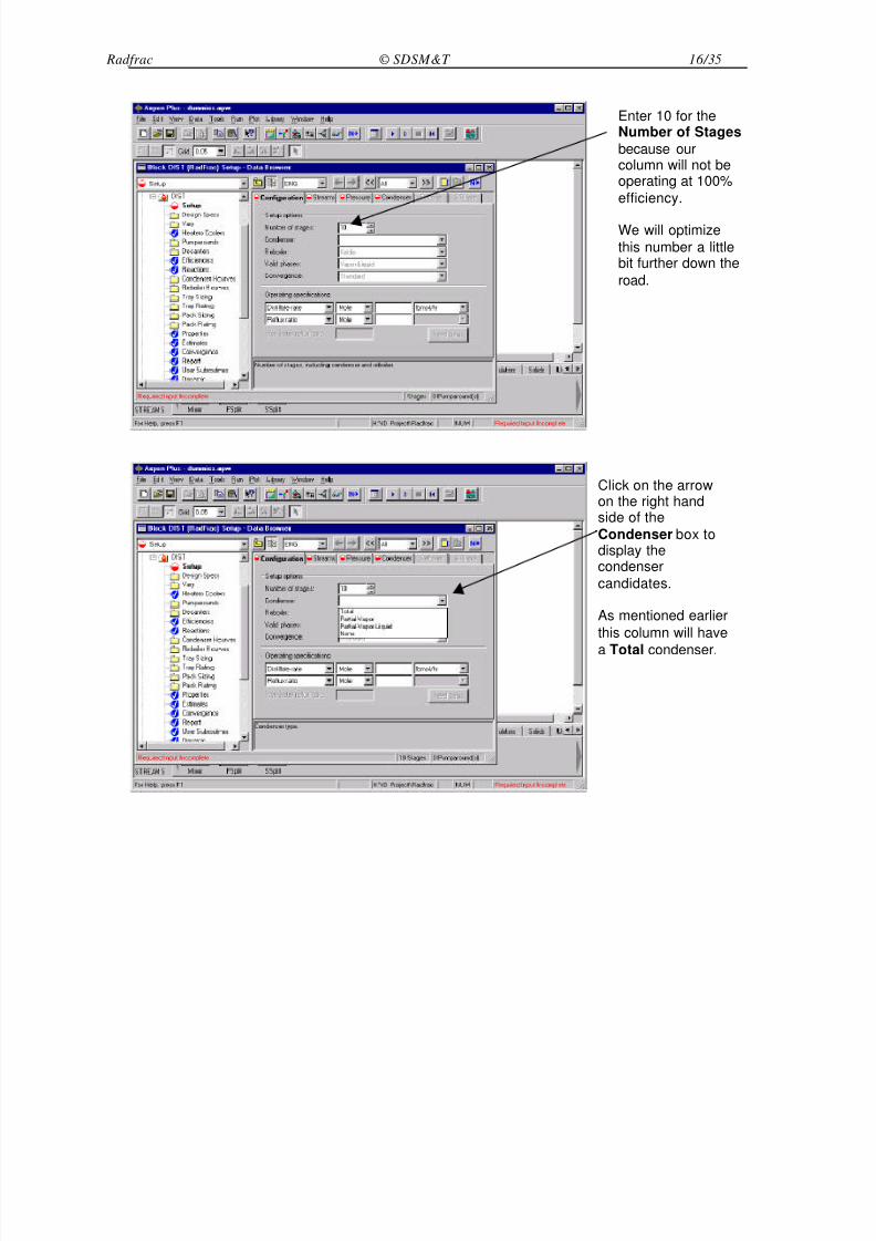
This diagram can
give us an estimateof how manyequilibrium stages
are necessary byusing the McCabe-Thiele method.
Unfortunately, wecannot show you
the actual drawingbut trust us; ittakes about 7
equilibrium stages.
After the graph has
been made andlooked at you canclose all three
windows that are
for the graph.
8/3/2019 Aspen Radfrac
http://slidepdf.com/reader/full/aspen-radfrac 16/35
Radfrac © SDSM&T 16/35
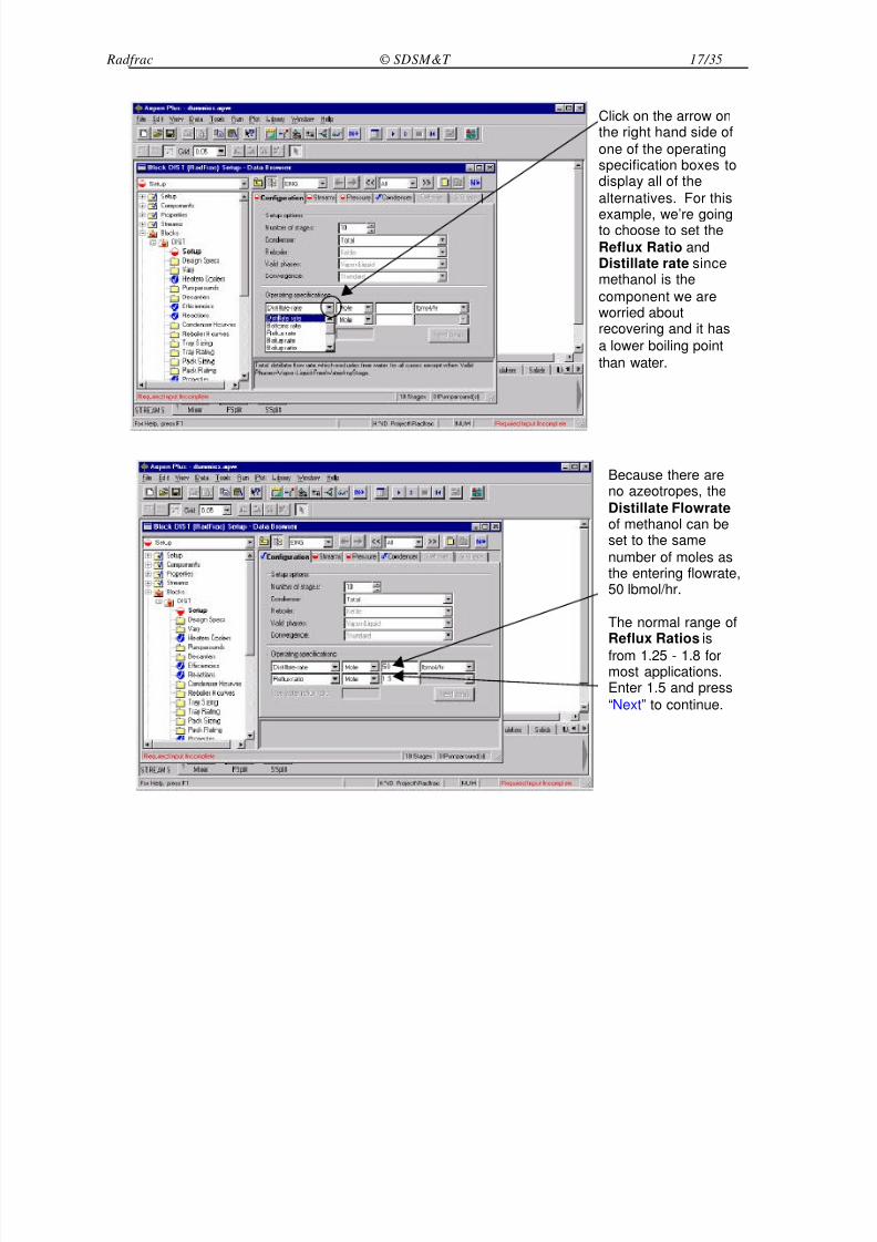
Enter 10 for theNumber of Stages
because ourcolumn will not beoperating at 100%
efficiency.
We will optimize
this number a littlebit further down the
road.
Click on the arrowon the right handside of the
Condenser box todisplay thecondenser
candidates.
As mentioned earlier
this column will have
a Total condenser.
8/3/2019 Aspen Radfrac
http://slidepdf.com/reader/full/aspen-radfrac 17/35
Radfrac © SDSM&T 17/35
Click on the arrow onthe right hand side of
one of the operatingspecification boxes todisplay all of the
alternatives. For this
example, we’re goingto choose to set the
Reflux Ratio andDistillate rate sincemethanol is the
component we areworried aboutrecovering and it has
a lower boiling point
than water.
Because there areno azeotropes, the
Distillate Flowrateof methanol can beset to the same
number of moles asthe entering flowrate,50 lbmol/hr.
The normal range ofReflux Ratios is
from 1.25 - 1.8 formost applications.Enter 1.5 and press
“Next” to continue.
8/3/2019 Aspen Radfrac
http://slidepdf.com/reader/full/aspen-radfrac 18/35
Radfrac © SDSM&T 18/35
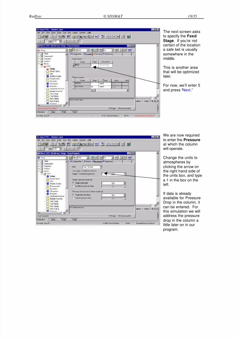
The next screen asksto specify the Feed
Stage. If you’re notcertain of the locationa safe bet is usually
somewhere in the
middle.
This is another areathat will be optimizedlater.
For now, we’ll enter 5
and press “Next.”
We are now required
to enter the Pressureat which the columnwill operate.
Change the units toatmospheres by
clicking the arrow onthe right hand side ofthe units box, and type
a 1 in the box on theleft.
If data is alreadyavailable for PressureDrop in the column, it
can be entered. Forthis simulation we willaddress the pressure
drop in the column alittle later on in our
program.
8/3/2019 Aspen Radfrac
http://slidepdf.com/reader/full/aspen-radfrac 19/35
Radfrac © SDSM&T 19/35
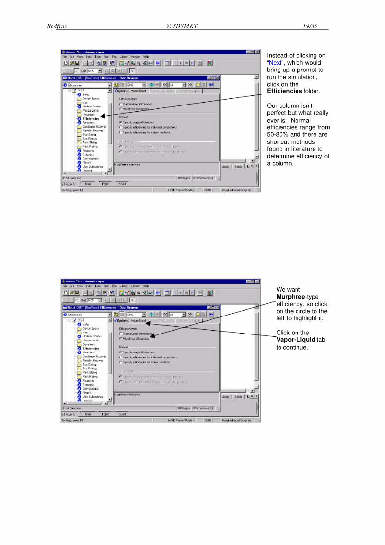
Instead of clicking on“Next”, which wouldbring up a prompt to
run the simulation,click on theEfficiencies folder.
Our column isn’tperfect but what really
ever is. Normalefficiencies range from50-80% and there are
shortcut methodsfound in literature todetermine efficiency of
a column.
We wantMurphree-type
efficiency, so clickon the circle to theleft to highlight it.
Click on theVapor-Liquid tab
to continue.
8/3/2019 Aspen Radfrac
http://slidepdf.com/reader/full/aspen-radfrac 20/35
Radfrac © SDSM&T 20/35
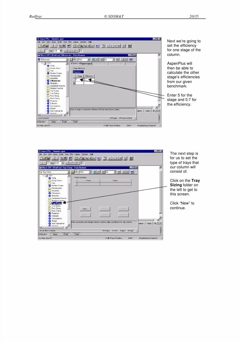
Next we’re going toset the efficiencyfor one stage of the
column.
AspenPlus will
then be able tocalculate the otherstage’s efficiencies
from our givenbenchmark.
Enter 5 for thestage and 0.7 for
the efficiency.
The next step isfor us to set the
type of trays thatour column willconsist of.
Click on the TraySizing folder on
the left to get tothis screen.
Click “New” to
continue.
8/3/2019 Aspen Radfrac
http://slidepdf.com/reader/full/aspen-radfrac 21/35
Radfrac © SDSM&T 21/35
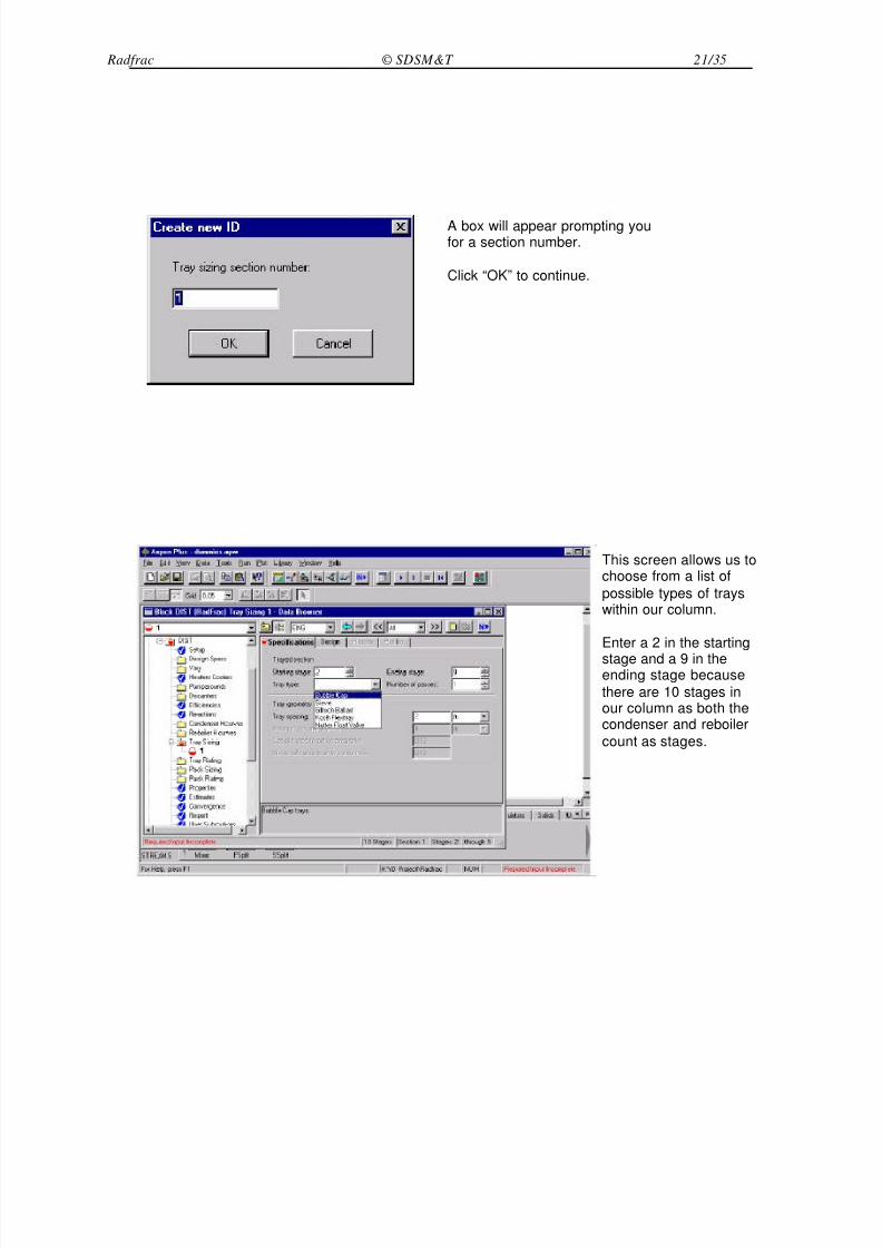
A box will appear prompting youfor a section number.
Click “OK” to continue.
This screen allows us tochoose from a list of
possible types of trayswithin our column.
Enter a 2 in the starting
stage and a 9 in theending stage because
there are 10 stages inour column as both thecondenser and reboiler
count as stages.
8/3/2019 Aspen Radfrac
http://slidepdf.com/reader/full/aspen-radfrac 22/35
Radfrac © SDSM&T 22/35
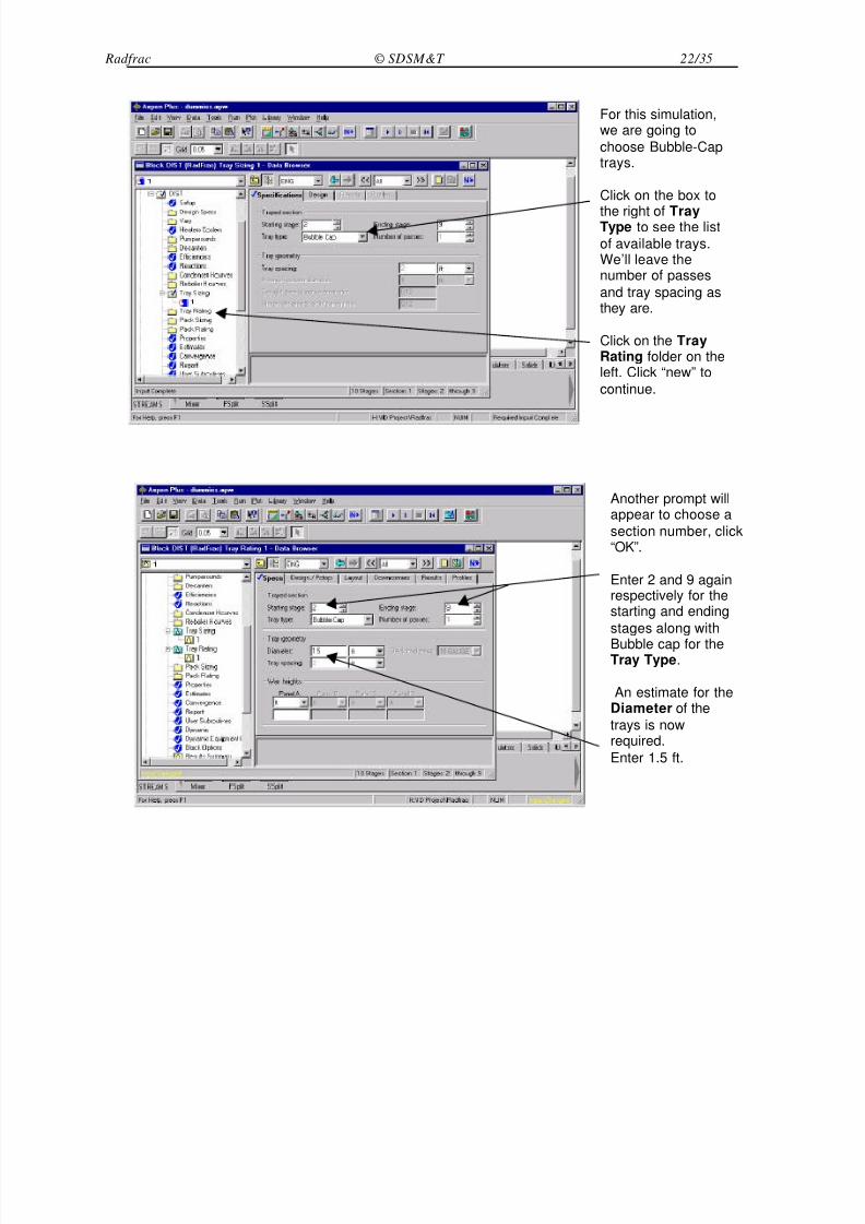
For this simulation,we are going to
choose Bubble-Captrays.
Click on the box to
the right of TrayType to see the list
of available trays.We’ll leave thenumber of passes
and tray spacing asthey are.
Click on the TrayRating folder on theleft. Click “new” to
continue.
Another prompt willappear to choose a
section number, click“OK”.
Enter 2 and 9 againrespectively for thestarting and ending
stages along with
Bubble cap for theTray Type.
An estimate for theDiameter of the
trays is nowrequired.
Enter 1.5 ft.
8/3/2019 Aspen Radfrac
http://slidepdf.com/reader/full/aspen-radfrac 23/35
Radfrac © SDSM&T 23/35
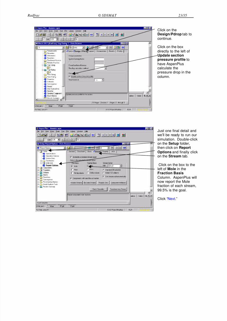
Click on theDesign/Pdrop tab to
continue.
Click on the box
directly to the left of
Update sectionpressure profile to
have AspenPluscalculate thepressure drop in the
column.
Just one final detail andwe’ll be ready to run our
simulation. Double-clickon the Setup folder,then click on Report
Options and finally clickon the Stream tab.
Click on the box to the
left of Mole in theFraction Basis
Column. AspenPlus willnow report the Molefraction of each stream,
99.5% is the goal.
Click “Next.”
8/3/2019 Aspen Radfrac
http://slidepdf.com/reader/full/aspen-radfrac 24/35
Radfrac © SDSM&T 24/35
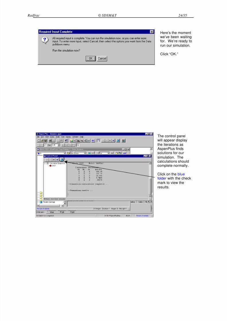
Here’s the momentwe’ve been waitingfor. We’re ready to
run our simulation.
Click “OK.”
The control panelwill appear display
the iterations asAspenPlus findssolutions for our
simulation. Thecalculations shouldcomplete normally.
Click on the bluefolder with the check
mark to view the
results.
8/3/2019 Aspen Radfrac
http://slidepdf.com/reader/full/aspen-radfrac 25/35
Radfrac © SDSM&T 25/35
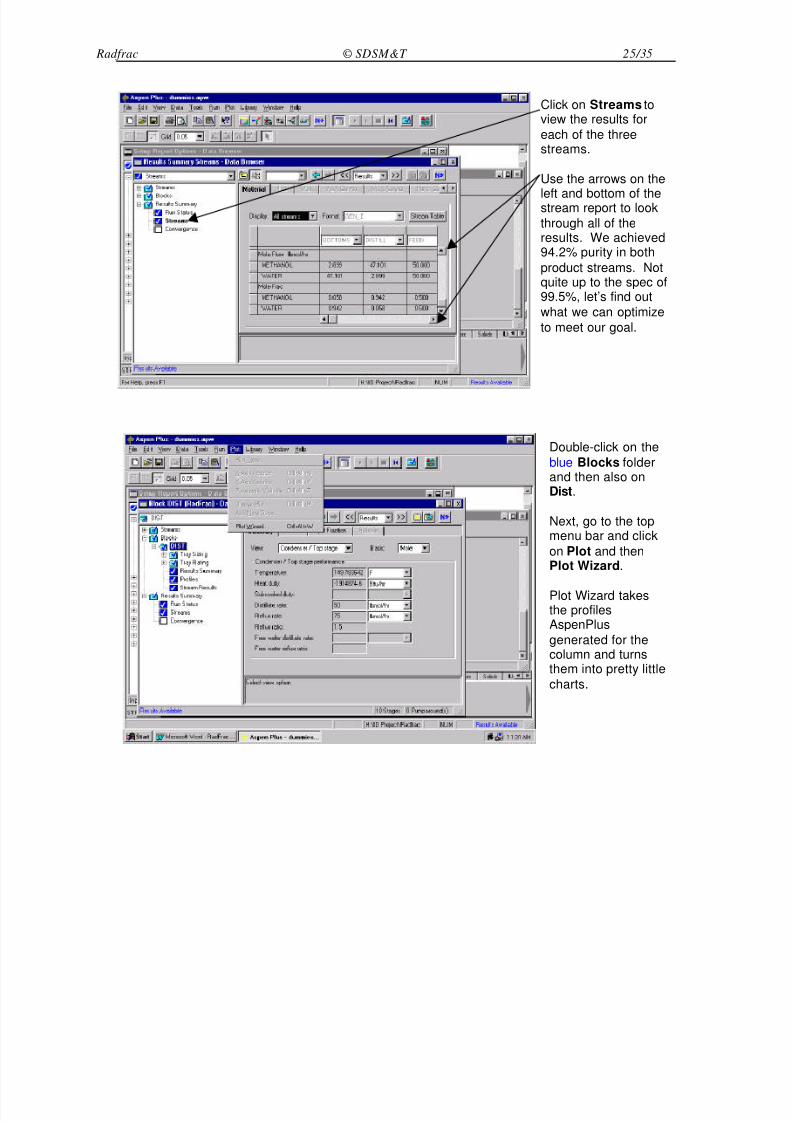
Click on Streams toview the results for
each of the threestreams.
Use the arrows on the
left and bottom of thestream report to look
through all of theresults. We achieved94.2% purity in both
product streams. Notquite up to the spec of99.5%, let’s find out
what we can optimize
to meet our goal.
Double-click on the
blue Blocks folderand then also onDist.
Next, go to the topmenu bar and click
on Plot and thenPlot Wizard.
Plot Wizard takesthe profilesAspenPlus
generated for thecolumn and turnsthem into pretty little
charts.
8/3/2019 Aspen Radfrac
http://slidepdf.com/reader/full/aspen-radfrac 26/35
Radfrac © SDSM&T 26/35
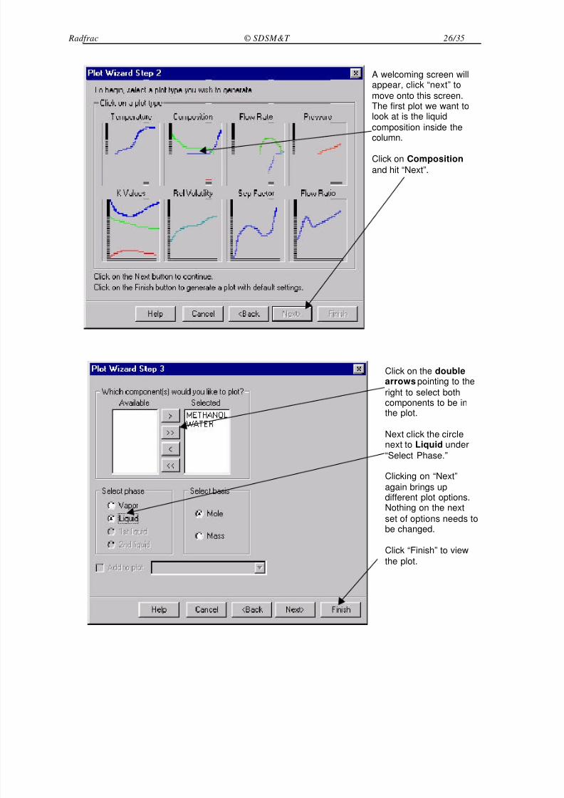
A welcoming screen willappear, click “next” to
move onto this screen.The first plot we want tolook at is the liquid
composition inside the
column.
Click on Composition
and hit “Next”.
Click on the doublearrows pointing to the
right to select bothcomponents to be inthe plot.
Next click the circlenext to Liquid under
“Select Phase.”
Clicking on “Next”
again brings updifferent plot options.Nothing on the next
set of options needs tobe changed.
Click “Finish” to view
the plot.
8/3/2019 Aspen Radfrac
http://slidepdf.com/reader/full/aspen-radfrac 27/35
Radfrac © SDSM&T 27/35
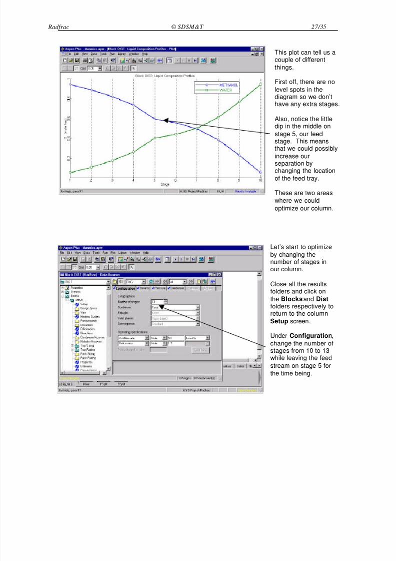
This plot can tell us acouple of different
things.
First off, there are no
level spots in the
diagram so we don’thave any extra stages.
Also, notice the littledip in the middle on
stage 5, our feedstage. This meansthat we could possibly
increase ourseparation bychanging the location
of the feed tray.
These are two areas
where we could
optimize our column.
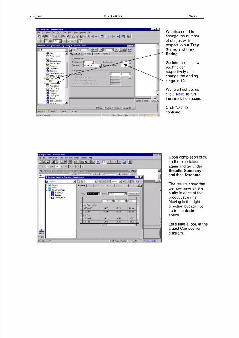
Let’s start to optimize
by changing thenumber of stages inour column.
Close all the resultsfolders and click on
the Blocks and Distfolders respectively toreturn to the column
Setup screen.
Under Configuration,
change the number ofstages from 10 to 13while leaving the feed
stream on stage 5 for
the time being.
8/3/2019 Aspen Radfrac
http://slidepdf.com/reader/full/aspen-radfrac 28/35
Radfrac © SDSM&T 28/35
We also need tochange the number
of stages withrespect to our TraySizing and Tray
Rating.
Go into the 1 below
each folderrespectively andchange the ending
stage to 12.
We’re all set up, so
click “Next” to runthe simulation again.
Click “OK” to
continue.
Upon completion clickon the blue folder
again and go underResults Summaryand then Streams.
The results show thatwe now have 94.9%
purity in each of theproduct streams.Moving in the right
direction but still notup to the desiredspecs.
Let’s take a look at theLiquid Composition
diagram…
8/3/2019 Aspen Radfrac
http://slidepdf.com/reader/full/aspen-radfrac 29/35
Radfrac © SDSM&T 29/35
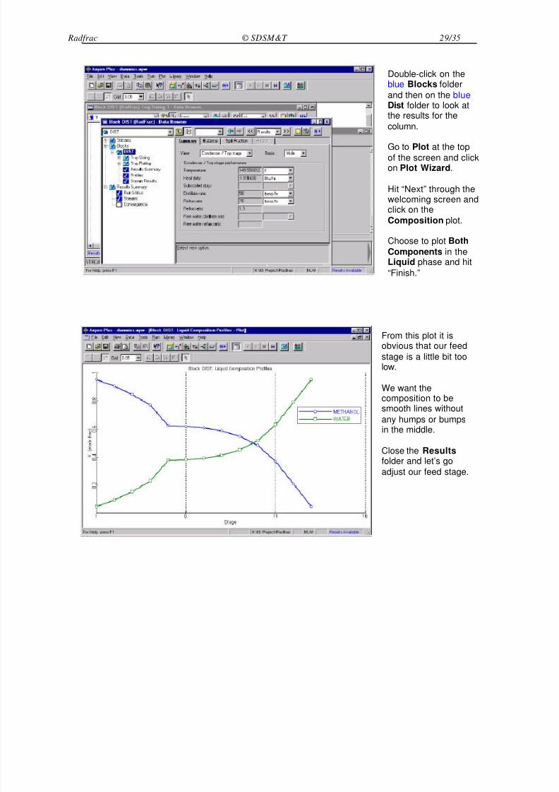
Double-click on theblue Blocks folder
and then on the blueDist folder to look atthe results for the
column.
Go to Plot at the top
of the screen and clickon Plot Wizard.
Hit “Next” through thewelcoming screen andclick on the
Composition plot.
Choose to plot Both
Components in theLiquid phase and hit
“Finish.”
From this plot it isobvious that our feed
stage is a little bit toolow.
We want thecomposition to besmooth lines without
any humps or bumpsin the middle.
Close the Resultsfolder and let’s go
adjust our feed stage.
8/3/2019 Aspen Radfrac
http://slidepdf.com/reader/full/aspen-radfrac 30/35
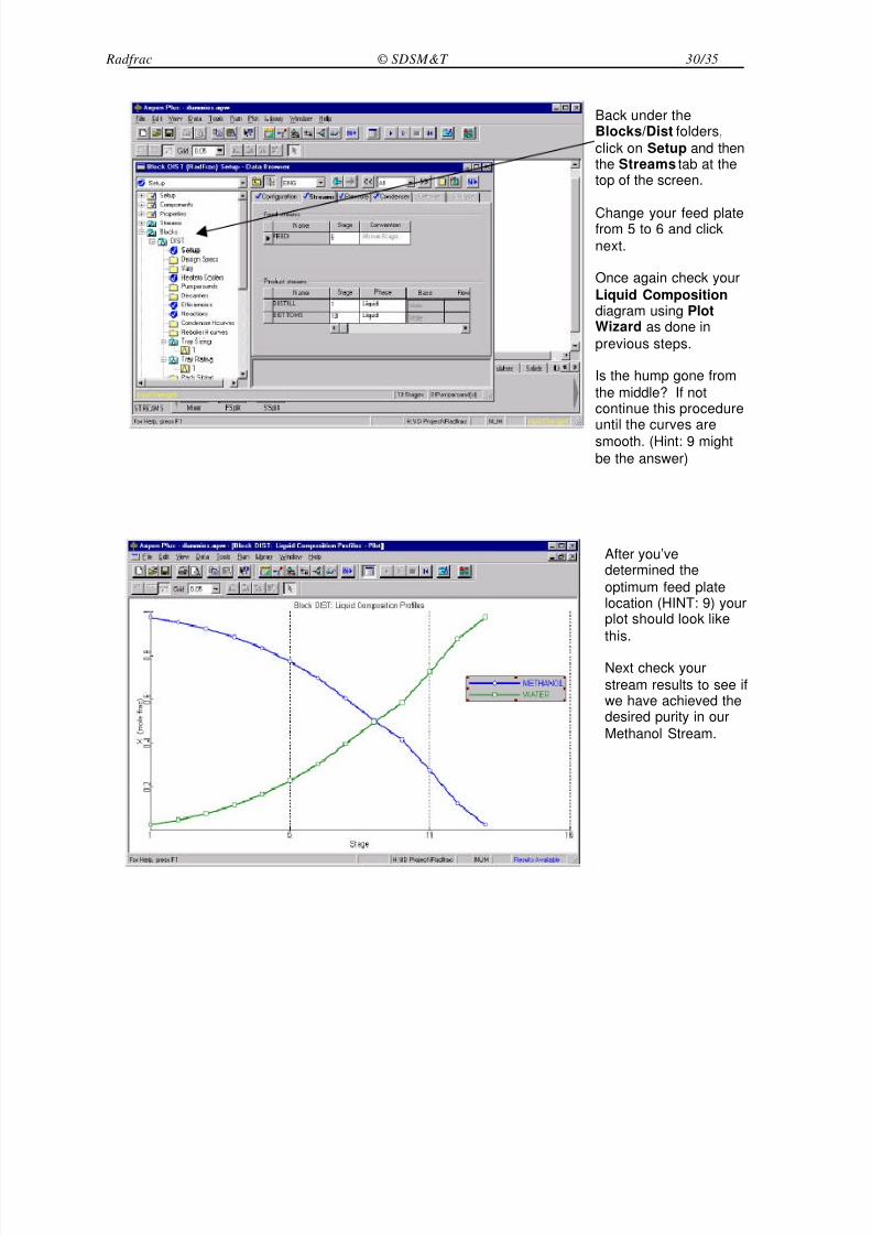
Radfrac © SDSM&T 30/35
Back under theBlocks/Dist folders,
click on Setup and thenthe Streams tab at thetop of the screen.
Change your feed platefrom 5 to 6 and click
next.
Once again check your
Liquid Compositiondiagram using PlotWizard as done in
previous steps.
Is the hump gone from
the middle? If notcontinue this procedureuntil the curves are
smooth. (Hint: 9 might
be the answer)
After you’vedetermined the
optimum feed platelocation (HINT: 9) yourplot should look like
this.
Next check your
stream results to see ifwe have achieved thedesired purity in our
Methanol Stream.
8/3/2019 Aspen Radfrac
http://slidepdf.com/reader/full/aspen-radfrac 31/35
Radfrac © SDSM&T 31/35
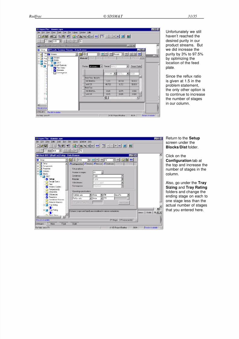
Unfortunately we stillhaven’t reached the
desired purity in ourproduct streams. Butwe did increase the
purity by 3% to 97.5%
by optimizing thelocation of the feed
plate.
Since the reflux ratio
is given at 1.5 in theproblem statement,the only other option is
to continue to increasethe number of stages
in our column.
Return to the Setupscreen under the
Blocks/Dist folder.
Click on the
Configuration tab atthe top and increase thenumber of stages in the
column.
Also, go under the Tray
Sizing and Tray Ratingfolders and change theending stage on each to
one stage less than theactual number of stages
that you entered here.
8/3/2019 Aspen Radfrac
http://slidepdf.com/reader/full/aspen-radfrac 32/35
Radfrac © SDSM&T 32/35
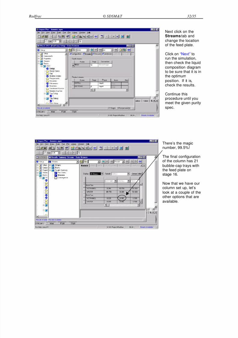
Next click on theStreams tab and
change the locationof the feed plate.
Click on “Next” to
run the simulation,then check the liquid
composition diagramto be sure that it is inthe optimum
position. If it is,check the results.
Continue thisprocedure until youmeet the given purity
spec.
There’s the magicnumber, 99.5%!
The final configurationof the column has 21
bubble-cap trays withthe feed plate onstage 16.
Now that we have ourcolumn set up, let’s
look at a couple of theother options that are
available.
8/3/2019 Aspen Radfrac
http://slidepdf.com/reader/full/aspen-radfrac 33/35
Radfrac © SDSM&T 33/35
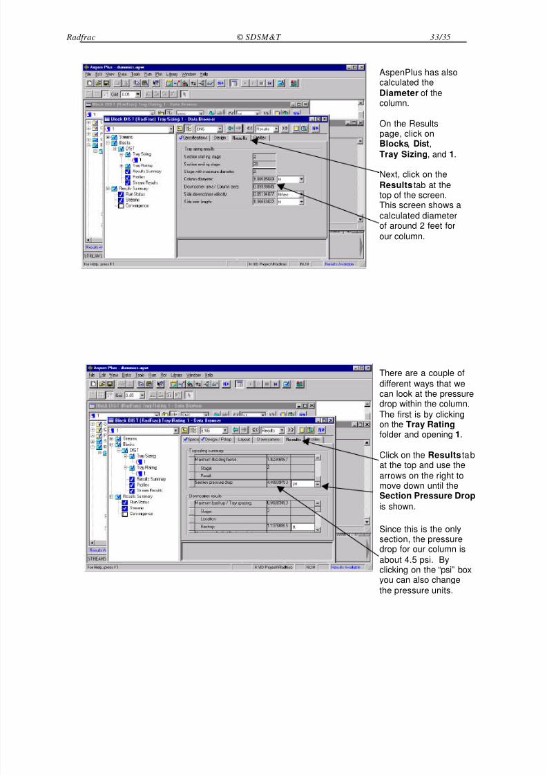
AspenPlus has alsocalculated the
Diameter of thecolumn.
On the Results
page, click onBlocks, Dist,
Tray Sizing, and 1.
Next, click on the
Results tab at thetop of the screen.This screen shows a
calculated diameterof around 2 feet for
our column.
There are a couple of
different ways that wecan look at the pressure
drop within the column.The first is by clickingon the Tray Ratingfolder and opening 1.
Click on the Results tabat the top and use the
arrows on the right tomove down until theSection Pressure Drop
is shown.
Since this is the only
section, the pressuredrop for our column is
about 4.5 psi. Byclicking on the “psi” boxyou can also change
the pressure units.
8/3/2019 Aspen Radfrac
http://slidepdf.com/reader/full/aspen-radfrac 34/35
Radfrac © SDSM&T 34/35
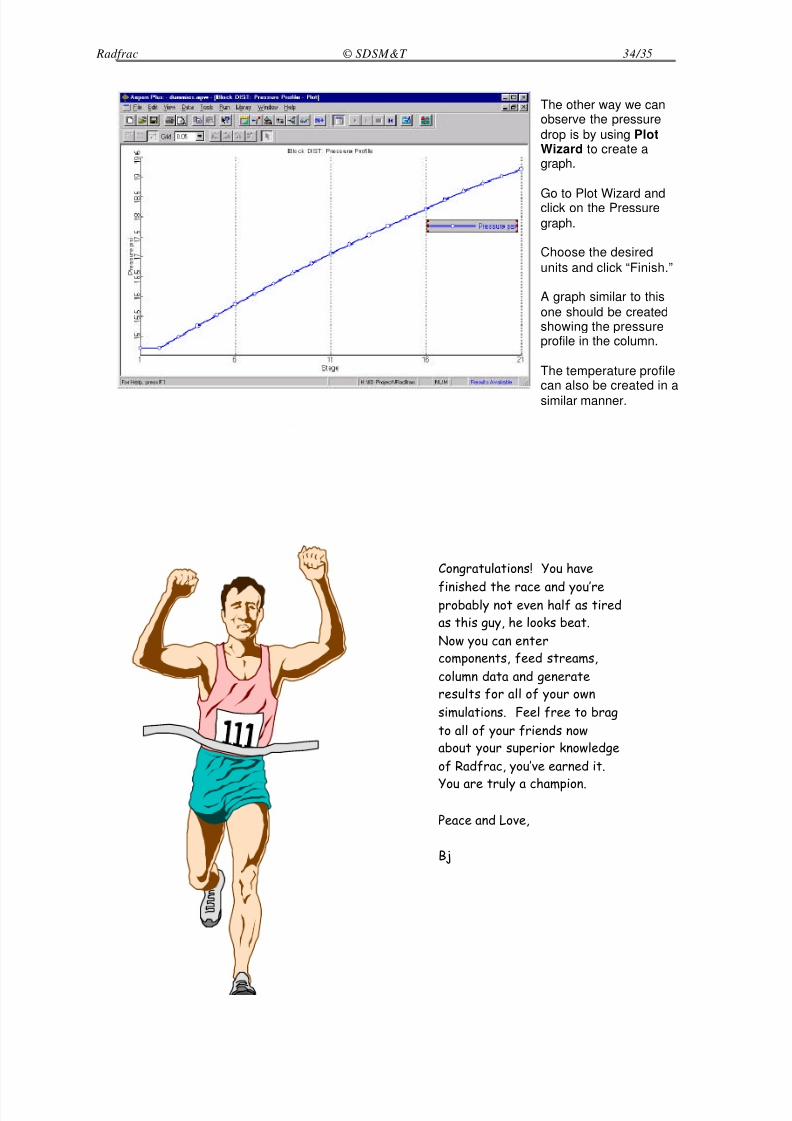
The other way we canobserve the pressure
drop is by using PlotWizard to create agraph.
Go to Plot Wizard andclick on the Pressure
graph.
Choose the desired
units and click “Finish.”
A graph similar to this
one should be createdshowing the pressureprofile in the column.
The temperature profilecan also be created in a
similar manner.
Congratulations! You have
finished the race and you’reprobably not even half as tired
as this guy, he looks beat.
Now you can enter
components, feed streams,
column data and generate
results for all of your own
simulations. Feel free to brag
to all of your friends now
about your superior knowledge
of Radfrac, you’ve earned it.
You are truly a champion.
Peace and Love,
Bj

8/3/2019 Aspen Radfrac
http://slidepdf.com/reader/full/aspen-radfrac 35/35
Radfrac © SDSM&T 35/35