Embed Size (px)
Citation preview
UNIVERSIDADE DE LISBOA
FACULDADE DE CIÊNCIAS
DEPARTAMENTO DE INFORMÁTICA
Automated Knowledge Extraction From ProteinSequence
Daniel Pedro de Jesus Faria
DOUTORAMENTO EM INFORMÁTICA
ESPECIALIDADE BIOINFORMÁTICA
2012

UNIVERSIDADE DE LISBOA
FACULDADE DE CIÊNCIAS
DEPARTAMENTO DE INFORMÁTICA
Automated Knowledge Extraction From ProteinSequence
Daniel Pedro de Jesus Faria
DOUTORAMENTO EM INFORMÁTICA
ESPECIALIDADE BIOINFORMÁTICA
Tese orientada pelo Dr. André Osório e Cruz de Azerêdo Falcão e pelo Dr.
António Eduardo do Nascimento Ferreira
2012


Resumo
Prever a função de proteínas a partir da sua sequência, de forma
precisa e e�ciente, é um dos problemas actuais da genética e bioin-
formática, sendo que os métodos para determinação experimental da
função não conseguem acompanhar o ritmo a que novas sequências
são publicadas.
A função das proteínas é condicionada pela sua estrutura tridimen-
sional, a qual depende da sequência, mas ainda não é possível modelar
esta informação com precisão su�ciente para fazer previsões funcionais
de novo. Assim, a previsão funcional de proteínas requer necessaria-
mente abordagens comparativas.
As abordagens mais comuns para prever a função de proteínas baseiam-
se em alinhamentos de sequência, e na suposição de que sequências
semelhantes evoluíram a partir de um ancestral comum e portanto
desempenharão funções semelhantes. No entanto, casos de evolução
divergente são relativamente comuns, e podem introduzir erros nestas
abordagens.
Abordagens de aprendizagem automática não envolvendo alinhamen-
tos foram já aplicadas para previsão funcional de proteínas, mas essen-
cialmente para prever aspectos funcionais genéricos.
A minha tese é que é possível extrair informação su�ciente da sequên-
cia de proteínas para prever aspectos funcionais detalhados de forma
precisa, sem recorrer a alinhamentos de sequência, e por conseguinte
desenvolver abordagens de aprendizagem automática capazes de com-
petir com as abordagens baseadas em alinhamentos.
Para demonstrar esta tese, desenvolvi e avaliei diversas abordagens
de aprendizagem automática no contexto de previsão funcional detal-
hada. Várias destas abordagens mostraram-se capazes de competir em
precisão com classi�cadores baseados em alinhamentos, e duas abor-
dagens superaram estes classi�cadores em problemas de classi�cação
de pequena dimensão. A principal contribuição do meu trabalho foi a
descoberta do poder informativo das sub-sequências tripeptídicas. A
composição de tripéptidos das sequências de proteínas deu origem aos
classi�cadores mais precisos de entre todas as abordagens testadas, e
permitiu mesmo comparar sequências directamente, como alternativa
aos alinhamentos de sequência.
Palavras Chave: Previsão Funcional de Proteínas, Aprendizagem
Automática, Máquinas de Vectores de Suporte, Gene Ontology, Ano-
tação
Abstract
E�cient and reliable prediction of protein functions based on their se-
quences is one of the standing problems in genetics and bioinformatics,
as experimental methods to determine protein function are unable to
keep up with the rate at which new sequences are published.
The function of a protein is conditioned by its three-dimensional struc-
ture, which is deeply tied to the sequence, but we cannot yet model
this information with su�cient reliability to make de novo protein
function predictions. Thus, protein function predictions are necessar-
ily comparative.
The most common approaches to protein function prediction rely on
sequence alignments and on the assumption that proteins of similar se-
quence have evolved from a common ancestor and thus should perform
similar functions. However, cases of divergent evolution are relatively
common, and can lead to prediction errors from these approaches.
Machine learning approaches not involving sequence alignments meth-
ods have also been applied to protein function prediction. However,
their application has been mostly restricted to predicting generic func-
tional aspects of proteins.
My thesis is that it is possible to extract su�cient information from
protein sequences to make reliable detailed function predictions with-
out the use of sequence alignments, and therefore develop machine
learning approaches that can compete in general with alignment-based
approaches.
To prove this thesis, I developed and evaluated multiple machine
learning approaches in the context of detailed function prediction.
Several of these approaches were able to compete with alignment-
based classi�ers in precision, and two outperformed them notably in
small classi�cation problems. The main contribution of my work was
the discovery of the informativeness of tripeptide subsequences. The
tripeptide composition of protein sequences not only led to the most
precise classi�cation of all approaches tested, but also was su�ciently
informative to measure similarity between proteins directly, and com-
pete with sequence alignments.
Keywords: Protein Function Prediction, Machine Learning, Support
Vector Machines, Gene Ontology, Annotation

Resumo Estendido
Prever a função de uma proteína a partir da sua sequência, de forma
precisa e e�ciente, é um dos problemas actuais da genética e bioin-
formática. Os métodos experimentais para determinar a função das
proteínas não conseguem acompanhar o ritmo a que novas sequên-
cias são publicadas, o que tem levado a uma crescente lacuna entre
sequência e função.
A função de uma proteína é condicionada pela sua estrutura tridi-
mensional, que por sua vez depende da sequência. No entanto, não é
ainda possível modelar esta informação com su�ciente precisão para
fazer previsões funcionais de novo. Assim sendo, a previsão da função
de uma proteína a partir da sua sequência requer necessariamente
uma abordagem comparativa.
As abordagens mais comuns para prever a função de proteínas baseiam-
se em alinhamentos de sequência, e na suposição de que sequências
semelhantes são homólogas (isto é, evoluíram de um ancestral co-
mum) e portanto devem desempenhar funções semelhantes. Assim, a
função de uma proteína é inferida a partir de proteínas de sequência
semelhante cuja função é conhecida, quer directamente, quer após o
agrupamento de sequências em famílias. Apesar da sua popularidade,
estas abordagens são inerentemente limitadas. Por um lado, têm di-
�culdade em capturar proteínas que partilham a mesma função mas
têm uma semelhança de sequência baixa (homologia remota). Por
outro lado, são induzidas em erro por casos de proteínas que, ape-
sar de terem sequências muito semelhantes, divergiram para realizar
funções diferentes.
Como alternativa às abordagens baseadas em alinhamentos, foram
já aplicadas abordagens de aprendizagem automática não evolvendo
alinhamentos para prever a função de proteínas. No entanto, estas

abordagens têm-se concentrado essencialmente na previsão de aspec-
tos funcionais genéricos, explorando os casos de homologia remota nos
quais as abordagens baseadas em alinhamentos têm di�culdades. Adi-
cionalmente, a maioria dos métodos de aprendizagem automática não
consegue lidar directamente com sequências de proteínas, precisando
de dados com um número �xo de atributos. A perda de informação
que resulta de converter sequências em vectores de atributos contribui
para limitar a aplicabilidade destes métodos a problemas de previsão
funcional genérica. Outra limitação destas abordagens é a sua ca-
pacidade limitada para lidar com dados em grande escala, que leva a
que sejam aplicadas apenas a sub-conjuntos relativamente pequenos
do universo de proteínas.
A minha tese é que é possível extrair informação su�ciente da sequên-
cia de proteínas para prever aspectos funcionais detalhados de forma
precisa, sem recorrer a alinhamentos de sequência, e por conseguinte
desenvolver abordagens de aprendizagem automática capazes de com-
petir de forma geral com as abordagens baseadas em alinhamentos.
Para demonstrar esta tese, desenvolvi e avaliei diversas abordagens
de aprendizagem automática no contexto da previsão detalhada de
funções. Adicionalmente, explorei o espaço funcional das proteínas
através das anotações da Gene Ontology, com o intuito de compreen-
der os limites da previsão funcional.
Fiz inicialmente uma avaliação em grande escala do uso de medidas de
semelhança semântica para comparar proteínas a nível funcional com
base nas suas anotações, uma vez que é essencial fazer comparações
funcionais para avaliar a qualidade das previsões funcionais. Adi-
cionalmente, comparar proteínas funcionalmente permitiu-me mode-
lar a relação entre a semelhança funcional e a semelhança de sequência,
e dessa forma estudar as limitações da previsão funcional com base em
alinhamentos de sequência. Identi�quei com esta avaliação a medida
simGIC como a mais adequada para medir a semelhança funcional
entre proteínas.
Realizei também um estudo sobre a consistência das anotações fun-
cionais das proteínas, que é um problema crítico para a previsão fun-
cional. O facto de que proteínas com a mesma função muitas vezes
não estão descritas com o mesmo conjunto de anotações compromete
a qualidade das abordagens de previsão funcional e di�culta a sua
avaliação. Neste contexto, desenvolvi um algoritmo de prospecção de
dados, baseado na metodologia de regras de associação, para descobrir
relações implícitas entre termos da Gene Ontology. Este algoritmo
pode não só ser aplicado para corrigir inconsistências nas anotações
existentes, como também para aumentar a consistência de novas pre-
visões funcionais.
Já no contexto da previsão funcional detalhada, desenvolvi e avaliei a
metodologia de aprendizagem automática Programas Peptídicos, re-
centemente concebida especi�camente para classi�cação funcional de
proteínas. O aspecto inovador desta metodologia é o facto de que
lida directamente com sequências de proteínas, modelando-as como
pequenos programas de computador. Avaliei os Programas Peptídi-
cos em 18 problemas de classi�cação binária detalhada, variando em
dimensão entre 400 e mais de 7000 proteinas. A minha avaliação
demonstrou que os Programas Peptídicos conseguem competir com
classi�cadores baseados em alinhamentos de sequência em problemas
de pequena dimensão (até 1500 proteínas). Todavia, devido à com-
plexidade do espaço de soluções, o seu desempenho piora gradual-
mente com o aumento da dimensão dos problemas de classi�cação.
Outro aspecto que diminui a aplicabilidade desta metodologia é o
facto de que o seu tempo de treino é muito elevado comparado com
as abordagens de aprendizagem automática estabelecidas.
Também no contexto da previsão funcional detalhada, avaliei o poder
informativo de diversas representações vectoriais de proteínas enquanto
atributos para classi�cação funcional. Testei todas as representações
com uma metodologia estabelecida de aprendizagem automática, as
máquinas de vectores de suporte, e testei também as representações

mais simples com uma metodologia para classi�cação linear que de-
senvolvi, chamada Programas Vectoriais. Uma das representações que
produziu melhores resultados foi a composição local de aminoácidos.
Em conjunção com os Programas Vectoriais, esta representação origi-
nou os melhores resultados em problemas de classi�cação de pequena
dimensão, a par com os Programas Peptídicos, mas com um tempo
de treino muito inferior. No global, a representação que originou os
melhores resultados foi a composição de tripéptidos. Utilizando esta
representação, as máquinas de vectores de suporte igualaram ou su-
peraram a precisão dos classi�cadores baseados em alinhamentos em
todos os problemas de classi�cação testados. Adicionalmente, esta
representação mostrou-se su�cientemente informativa para medir di-
rectamente a semelhança entre proteínas. A medida de semelhança
de proteinas baseada nesta representação, TripSim, originou resulta-
dos de classi�cação idênticos ou ligeiramente superiores aos obtidos
com alinhamentos de sequência, utilizando os mesmos algoritmos de
vizinhos mais próximos.
Avaliei adicionalmente a medida TripSim numa tarefa de previsão
funcional que replica o uso típico das abordagens baseadas em al-
inhamentos de sequência. Para cada proteína de um conjunto de
teste de 148 proteínas, a tarefa consistia em prever todas as suas ano-
tações funcionais (incluindo anotações detalhadas), tendo como con-
junto de treino todo o universo de proteínas. Também nesta tarefa,
os classi�cadores utilizando TripSim tiveram resultados idênticos ou
ligeiramente superiores aos classi�cadores utilizando alinhamentos de
sequência. Dados estes resultados, a medida TripSim será uma al-
ternativa viável aos algoritmos de alinhamento de sequência para en-
contrar proteínas semelhantes, particularmente tendo em conta que é
computacionalmente mais simples.
Finalmente, desenvolvi e avaliei um algoritmo de previsão funcional
híbrido, chamado TriGOPred, que combina uma busca por proteínas
semelhantes baseada na medida TripSim com máquinas de vectores
de suporte baseadas na composição de tripéptidos. O pressuposto
por trás deste algoritmo é que utilizar máquinas de vectores de su-
porte para a classi�cação é mais �ável do que empregar estratégias
de vizinhos mais próximos, como demonstraram os resultados obtidos
com as máquinas de vectores de suporte baseadas na composição de
tripéptidos. No entanto, dado que não é possível aplicar máquinas de
vectores de suporte a todo o universo de proteínas, é necessário reduzir
a escala dos problemas de previsão funcional. Este algoritmo tira par-
tido da medida de semelhança TripSim para localizar a proteína no
espaço de sequências, e reduzir a escala do problema à vizinhança lo-
cal da proteína. Assim, as máquinas de vectores de suporte apenas
têm de modelar o problema a nível local, utilizando as proteínas da
vizinhança como conjunto de treino.
O desempenho do algoritmo TriGOPred na tarefa de previsão fun-
cional foi igual ou superior ao de classi�cadores de vizinho mais próx-
imo, quer baseados em alinhamentos de sequência, quer baseados
na medida TripSim. Adicionalmente, apesar de requerer o treino
de máquinas de vectores de suporte para cada previsão, o algoritmo
TriGOPred tem um tempo de execução que compete com o da maioria
das ferramentas de previsão funcional. Assim, este algoritmo é uma
abordagem prática e �ável para previsão funcional de proteínas.

Acknowledgements
This thesis re�ects several years of research work, both individual and
collaborative, and ultimately a signi�cant part of my life. Many peo-
ple contributed directly to my work, while many others contributed
indirectly, and I am grateful for their help, support and company.
First, I would like to thank my supervisor, Doctor André Falcão, for
his guidance, support and not least for his unwavering energy and
optimism. Working closely with him was a previlege, as he always
had original research ideas, and readily encouraged some of my own.
Second, I would like to thank my co-supervisor, Doctor António Fer-
reira, also for his guidance and support. His critical revision of my re-
search from a biochemical perspective contributed greatly to its qual-
ity.
Third, I would like to thank Doctor Francisco Couto, who brought
me into the XLDB group and helped guide my research regarding the
Gene Ontology.
I am grateful for the funding of the Fundação para a Ciência e Tec-
nologia, through the PhD scholarship SFRH/BD/29797/2006, with-
out which my research would not have been possible.
My thanks to Professor Mário Silva for welcoming me into the XLDB
group and, together with Engineer Pedro Fernandes and Doctor Oc-
távio Paulo, for accepting me into the bioinformatics post-graduation
course that led directly to my PhD application. My thanks also to
Professor Isabel Sá Correia, who �rst got me interested in bioinfor-
matics.

I am very grateful to Cátia Pesquita, with whom I collaborated closely
in parts of my research, and whose discussions contributed invaluably
to the other parts.
I am grateful also for the help of Hugo Bastos and Andreas Schlicker,
who collaborated in parts of my research.
A special thanks to my visiting colleague Sebastian Köhler, the coolest
cat in town, who made research work seem exciting once again. Thanks
also to Tiago Grego, and all my other colleagues at the XLDB group,
who contributed to a great working environment.
I would also like to thank my friends, Miguel Gabriel, Ruben Carvalho,
João Ataíde and André Monteiro, for keeping things light when the
work got too heavy.
Finally, I would not be here today if not for the love, support and
inspiration of my family. My heart goes, in particular, to my parents,
my grandfather, my brother David and most of all, to my partner
Cátia Machado, who lifted me up when I was falling and never faltered
at my side.
Mínimo sou,
Mas quando ao Nada empresto
A minha elementar realidade,
O Nada é só o resto.
- Reinaldo Ferreira

Contents
1 Introduction 1
1.1 The Macromolecules of Life . . . . . . . . . . . . . . . . . . . . . 1
1.2 Historical Perspective . . . . . . . . . . . . . . . . . . . . . . . . . 2
1.3 Protein Function Prediction . . . . . . . . . . . . . . . . . . . . . 4
1.4 Thesis and Contributions . . . . . . . . . . . . . . . . . . . . . . . 6
2 State of the Art 9
2.1 About Proteins . . . . . . . . . . . . . . . . . . . . . . . . . . . . 9
2.1.1 Amino Acids . . . . . . . . . . . . . . . . . . . . . . . . . 9
2.1.2 Sequence . . . . . . . . . . . . . . . . . . . . . . . . . . . . 10
2.1.3 Three-Dimensional Structure . . . . . . . . . . . . . . . . 10
2.1.4 Function . . . . . . . . . . . . . . . . . . . . . . . . . . . . 11
2.2 Protein Resources . . . . . . . . . . . . . . . . . . . . . . . . . . . 12
2.2.1 The UniProt Knowledge Base . . . . . . . . . . . . . . . . 12
2.2.2 The Worldwide Protein Data Bank . . . . . . . . . . . . . 12
2.2.3 The Enzyme Commission System . . . . . . . . . . . . . . 13
2.2.4 The Gene Ontology . . . . . . . . . . . . . . . . . . . . . . 14
2.2.5 The InterPro . . . . . . . . . . . . . . . . . . . . . . . . . 15
2.3 Alignment-Based Protein Function Prediction . . . . . . . . . . . 16
2.3.1 Alignment-Based Inference . . . . . . . . . . . . . . . . . . 16
2.3.2 Signature-Based Classi�cation . . . . . . . . . . . . . . . . 18
2.4 Machine Learning Approaches for Protein Function Prediction . . 19
2.4.1 Support Vector Machines . . . . . . . . . . . . . . . . . . . 19
2.4.2 Sequence Representations . . . . . . . . . . . . . . . . . . 20
2.4.3 Application Issues . . . . . . . . . . . . . . . . . . . . . . . 21
xv
CONTENTS
3 Measuring Functional Similarity Between Proteins 23
3.1 Background . . . . . . . . . . . . . . . . . . . . . . . . . . . . . . 23
3.2 Methods . . . . . . . . . . . . . . . . . . . . . . . . . . . . . . . . 24
3.2.1 Dataset . . . . . . . . . . . . . . . . . . . . . . . . . . . . 24
3.2.2 Sequence Similarity Measures . . . . . . . . . . . . . . . . 25
3.2.3 Semantic Similarity Measures . . . . . . . . . . . . . . . . 26
3.2.4 Data Processing and Modelling . . . . . . . . . . . . . . . 28
3.3 The Relationship Between Functional Similarity and Sequence Sim-
ilarity . . . . . . . . . . . . . . . . . . . . . . . . . . . . . . . . . 28
3.3.1 Modelling . . . . . . . . . . . . . . . . . . . . . . . . . . . 28
3.4 Evaluating Semantic Similarity Measures . . . . . . . . . . . . . . 35
3.4.1 Evaluation Criterion . . . . . . . . . . . . . . . . . . . . . 35
3.4.2 Combination Strategies . . . . . . . . . . . . . . . . . . . . 36
3.4.3 Semantic Similarity Measures . . . . . . . . . . . . . . . . 40
3.5 Discussion . . . . . . . . . . . . . . . . . . . . . . . . . . . . . . . 44
3.5.1 Electronic versus Manually Curated Annotations . . . . . 44
3.5.2 Sequence Similarity Measures . . . . . . . . . . . . . . . . 44
3.5.3 The Relationship Between Sequence and Function . . . . . 45
3.5.4 Term Similarity Combination Strategies . . . . . . . . . . 45
3.5.5 Semantic Similarity Measures . . . . . . . . . . . . . . . . 46
4 Improving Annotation Consistency 49
4.1 Background . . . . . . . . . . . . . . . . . . . . . . . . . . . . . . 49
4.2 Methods . . . . . . . . . . . . . . . . . . . . . . . . . . . . . . . . 51
4.2.1 Dataset . . . . . . . . . . . . . . . . . . . . . . . . . . . . 51
4.2.2 Redundant Annotations . . . . . . . . . . . . . . . . . . . 51
4.2.3 Incomplete Annotations . . . . . . . . . . . . . . . . . . . 51
4.2.4 MFclasses . . . . . . . . . . . . . . . . . . . . . . . . . . . 52
4.2.5 Inconsistent Annotations . . . . . . . . . . . . . . . . . . . 53
4.2.6 Association Rule Learning . . . . . . . . . . . . . . . . . . 53
4.2.7 GO Relationship Learning Version 1 . . . . . . . . . . . . 54
4.2.8 GO Relationship Learning Version 2 . . . . . . . . . . . . 57
4.2.9 Evaluation of the GRL algorithms . . . . . . . . . . . . . . 57
xvi

CONTENTS
4.3 Exploring the Annotation Space . . . . . . . . . . . . . . . . . . . 58
4.3.1 Redundant Annotations and Incomplete Annotations . . . 58
4.3.2 De�ning Protein Function . . . . . . . . . . . . . . . . . . 59
4.3.3 Inconsistent Annotations . . . . . . . . . . . . . . . . . . . 61
4.4 Finding Relationships Between Molecular Function Terms . . . . 65
4.4.1 GO Relationship Learning Results . . . . . . . . . . . . . . 65
4.4.2 Comparison with Association Rule Learning . . . . . . . . 65
4.4.3 Discussion . . . . . . . . . . . . . . . . . . . . . . . . . . . 67
5 Detailed Enzyme Classi�cation with Peptide Programs 69
5.1 Background . . . . . . . . . . . . . . . . . . . . . . . . . . . . . . 69
5.2 Methods . . . . . . . . . . . . . . . . . . . . . . . . . . . . . . . . 70
5.2.1 Enzyme Classi�cation Datasets . . . . . . . . . . . . . . . 70
5.2.2 Peptide Program Framework . . . . . . . . . . . . . . . . . 73
5.2.3 Peptide Program Training . . . . . . . . . . . . . . . . . . 75
5.2.4 Peptide Program Implementation and Development . . . . 77
5.2.5 Alignment-Based Benchmark . . . . . . . . . . . . . . . . 78
5.2.6 Machine Learning Benchmark . . . . . . . . . . . . . . . . 80
5.2.7 Evaluation Parameters . . . . . . . . . . . . . . . . . . . . 82
5.3 Peptide Program Evaluation . . . . . . . . . . . . . . . . . . . . . 83
5.3.1 Peptide Program Classi�cation Results . . . . . . . . . . . 83
5.3.2 BLAST Classi�cation Results . . . . . . . . . . . . . . . . 84
5.3.3 Property SVM Classi�cation Results . . . . . . . . . . . . 86
5.3.4 Peptide Programs versus BLAST . . . . . . . . . . . . . . 86
5.3.5 Peptide Programs versus Property SVMs . . . . . . . . . . 88
5.4 Discussion . . . . . . . . . . . . . . . . . . . . . . . . . . . . . . . 88
6 Exploring Sequence Representations 91
6.1 Background . . . . . . . . . . . . . . . . . . . . . . . . . . . . . . 91
6.2 Methods . . . . . . . . . . . . . . . . . . . . . . . . . . . . . . . . 92
6.2.1 Datasets and Benchmarks . . . . . . . . . . . . . . . . . . 92
6.2.2 Sequence Representations . . . . . . . . . . . . . . . . . . 92
6.2.3 Support Vector Machines . . . . . . . . . . . . . . . . . . . 94
6.2.4 Vector Programs . . . . . . . . . . . . . . . . . . . . . . . 94
xvii
CONTENTS
6.2.5 Alignment-Based Benchmark . . . . . . . . . . . . . . . . 95
6.2.6 Tripeptide-Based Similarity . . . . . . . . . . . . . . . . . 95
6.2.7 Evaluation Parameters . . . . . . . . . . . . . . . . . . . . 96
6.3 Testing Sequence Representations . . . . . . . . . . . . . . . . . . 96
6.3.1 Global and Local Amino Acid Composition . . . . . . . . . 96
6.3.2 Dipeptide and Tripeptide Composition . . . . . . . . . . . 98
6.3.3 TripSim Classi�cation . . . . . . . . . . . . . . . . . . . . 99
6.3.4 Size-Corrected TripSim Classi�cation . . . . . . . . . . . . 103
6.4 Discussion . . . . . . . . . . . . . . . . . . . . . . . . . . . . . . . 104
7 Predicting Molecular Function Annotations 109
7.1 Background . . . . . . . . . . . . . . . . . . . . . . . . . . . . . . 109
7.2 Methods . . . . . . . . . . . . . . . . . . . . . . . . . . . . . . . . 111
7.2.1 Dataset . . . . . . . . . . . . . . . . . . . . . . . . . . . . 111
7.2.2 Evaluation Criteria . . . . . . . . . . . . . . . . . . . . . . 111
7.2.3 BLAST Benchmark . . . . . . . . . . . . . . . . . . . . . . 112
7.2.4 TripSim Nearest Neighbors . . . . . . . . . . . . . . . . . . 113
7.2.5 TriGOPred Algorithm . . . . . . . . . . . . . . . . . . . . 114
7.3 Evaluating TripSim and TriGOPred . . . . . . . . . . . . . . . . . 115
7.3.1 BLAST Prediction Results . . . . . . . . . . . . . . . . . . 115
7.3.2 TripSim Prediction Results . . . . . . . . . . . . . . . . . . 116
7.3.3 TriGOPred Prediction Results . . . . . . . . . . . . . . . . 116
7.3.4 Comparison with Prediction Webtools . . . . . . . . . . . 117
7.3.5 Discussion . . . . . . . . . . . . . . . . . . . . . . . . . . . 117
8 Conclusions 119
A Manual Evaluation of the GO Relationship Learning Algorithms125
B EC Family Classi�cation Results 137
C Underrepresented and Overrepresented Dipeptides and Tripep-
tides in UniProtKB 149
D Molecular Function Annotation Prediction Results 153
xviii
CONTENTS
References 167
xix

List of Figures
3.1 Resnik's semantic similarity measure with the BMA approach as
function of the LRBS sequence similarity measure . . . . . . . . . 29
3.2 Resnik's semantic similarity measure with the BMA approach as
function of the RRBS sequence similarity measure . . . . . . . . . 30
3.3 Bimodal versus unimodal �t to Resnik's semantic similarity mea-
sure with the BMA approach versus LRBS sequence similarity. . . 32
3.4 Resnik's semantic similarity measure with the average approach as
function of the LRBS sequence similarity measure . . . . . . . . . 38
3.5 Resnik's semantic similarity measure with the maximum approach
as function of the LRBS sequence similarity measure . . . . . . . 39
3.6 Resnik's semantic similarity measure with the BMA and GraSM
approaches as function of the LRBS sequence similarity measure . 41
3.7 Comparison of the three term similarity measures using the BMA
approach as function of the LRBS sequence similarity measure . . 42
3.8 Comparison of the simGIC and simUI semantic similarity mea-
sures as function of the RRBS sequence similarity measure . . . . 43
4.1 Distribution of the number of terms per MFclasses. . . . . . . . . 60
4.2 Distribution of the usage frequency of MFclasses with power law
regression curve. . . . . . . . . . . . . . . . . . . . . . . . . . . . . 61
6.1 Average testing performance (Matthews correlation coe�cient) of
SVM and vector program (VP) classi�ers based on local amino
acid compositions, as function of the number of sequence divisions
considered. . . . . . . . . . . . . . . . . . . . . . . . . . . . . . . . 97
xxi

LIST OF FIGURES
6.2 Average TripSim values over intervals of 1% relative BLAST score. 102
xxii

List of Tables
3.1 Parameters of the modelling function for the full dataset and the
LRBS sequence similarity measure. . . . . . . . . . . . . . . . . . 33
3.2 Parameters of the modelling function for the full dataset and the
RRBS sequence similarity measure. . . . . . . . . . . . . . . . . . 34
3.3 Parameters of the modelling function for the non-electronic dataset
and the LRBS sequence similarity measure. . . . . . . . . . . . . . 34
3.4 Parameters of the modelling function for the non-electronic dataset
and the RRBS sequence similarity measure. . . . . . . . . . . . . 35
3.5 Resolution of each semantic similarity measure for each dataset
and sequence similarity measure. . . . . . . . . . . . . . . . . . . 37
5.1 Characterization of the enzyme family classi�cation datasets. . . . 73
5.2 Performance of Peptide Program classi�ers in detailed EC family
classi�cation tasks. . . . . . . . . . . . . . . . . . . . . . . . . . . 84
5.3 Performance of two BLAST classi�ers in detailed EC family clas-
si�cation tasks. . . . . . . . . . . . . . . . . . . . . . . . . . . . . 85
5.4 Performance of the property SVM classi�ers in detailed EC family
classi�cation tasks. . . . . . . . . . . . . . . . . . . . . . . . . . . 87
6.1 Performance of the dipeptide and tripeptide SVM classi�ers in
detailed EC family classi�cation tasks. . . . . . . . . . . . . . . . 100
6.2 Performance of two classi�ers based on the size-corrected TripSim
measure in EC family classi�cation tasks. . . . . . . . . . . . . . . 104
7.1 Average molecular function annotation prediction results with mul-
tiple approaches. . . . . . . . . . . . . . . . . . . . . . . . . . . . 115
xxiii

LIST OF TABLES
A.1 Manual evaluation of the top 100 relationships retrieved by the
GRL1 algorithm. . . . . . . . . . . . . . . . . . . . . . . . . . . . 125
A.2 Manual evaluation of the top 100 relationships retrieved by the
GRL2 algorithm. . . . . . . . . . . . . . . . . . . . . . . . . . . . 130
B.1 Performance of the composition SVM classi�ers in detailed EC
family classi�cation tasks. . . . . . . . . . . . . . . . . . . . . . . 137
B.2 Performance of composition vector program classi�ers in detailed
EC family classi�cation tasks. . . . . . . . . . . . . . . . . . . . . 138
B.3 Performance of the 2-part SVM classi�ers in detailed EC family
classi�cation tasks. . . . . . . . . . . . . . . . . . . . . . . . . . . 139
B.4 Performance of the 2-part vector program classi�ers in detailed EC
family classi�cation tasks. . . . . . . . . . . . . . . . . . . . . . . 140
B.5 Performance of the 4-part SVM classi�ers in detailed EC family
classi�cation tasks. . . . . . . . . . . . . . . . . . . . . . . . . . . 141
B.6 Performance of the 4-part vector program classi�ers in detailed EC
family classi�cation tasks. . . . . . . . . . . . . . . . . . . . . . . 142
B.7 Performance of the 6-part SVM classi�ers in detailed EC family
classi�cation tasks. . . . . . . . . . . . . . . . . . . . . . . . . . . 143
B.8 Performance of the 6-part vector program classi�ers in detailed EC
family classi�cation tasks. . . . . . . . . . . . . . . . . . . . . . . 144
B.9 Performance of the 8-part SVM classi�ers in detailed EC family
classi�cation tasks. . . . . . . . . . . . . . . . . . . . . . . . . . . 145
B.10 Performance of the 8-part vector program classi�ers in detailed EC
family classi�cation tasks. . . . . . . . . . . . . . . . . . . . . . . 146
B.11 Performance of two nearest-neighbors classi�ers based on the Trip-
Sim measure in detailed EC family classi�cation tasks. . . . . . . 147
C.1 Occurred versus expected ratio of the 20 most underrepresented
(left) and the 20 most overrepresented (right) dipeptides in UniPro-
tKB proteins. . . . . . . . . . . . . . . . . . . . . . . . . . . . . . 150
C.2 Occurred versus expected ratio of the 20 most underrepresented
(left) and the 20 most overrepresented (right) tripeptides in UniPro-
tKB proteins. . . . . . . . . . . . . . . . . . . . . . . . . . . . . . 151
xxiv
LIST OF TABLES
D.1 Molecular function annotation prediction results with two BLAST
classi�ers. . . . . . . . . . . . . . . . . . . . . . . . . . . . . . . . 153
D.2 Molecular function annotation prediction results with two TripSim
classi�ers. . . . . . . . . . . . . . . . . . . . . . . . . . . . . . . . 157
D.3 Molecular function annotation prediction results with the TriGO-
Pred algorithm using a BLAST or TripSim search. . . . . . . . . . 162
xxv


Chapter 1
Introduction
1.1 The Macromolecules of Life
Deoxyribonucleic acid (DNA) is the blueprint for all living organisms, encod-
ing the genetic instructions necessary for their development and sustenance. The
DNA of an organism includes both coding segments, called genes, and non-coding
segments, which play a role in regulating the expression of the genes. DNA is a
polymer composed by 4 distinct nucleotides, and it is the sequence of those nu-
cleotides in the DNA chain that encodes the genetic and regulatory information.
The �rst step in the gene expression process is the transcription of a DNA gene
into a ribonucleic acid (RNA) molecule, possibly followed by post-transcriptional
processing, depending on the organism and type of RNA. Similar to DNA, RNA
is a polymer composed by 4 distinct nucleotides, whose sequence is directly de-
termined by the DNA sequence of a gene through nucleotide complementarity.
For most genes, the RNA molecule is merely a portable copy of the gene, called
messenger RNA, which is used as a template to synthesize a protein. However,
some RNA molecules have an active role within the cell, and thus are the �-
nal products of the genes that encode them. The most important of these are
the ribosomal RNA and transfer RNA molecules, which are central pieces of the
protein synthesis process.
The second step of the gene expression process, for protein-coding genes, is
the translation process, wherein the messenger RNA molecule is translated into
1
1. INTRODUCTION
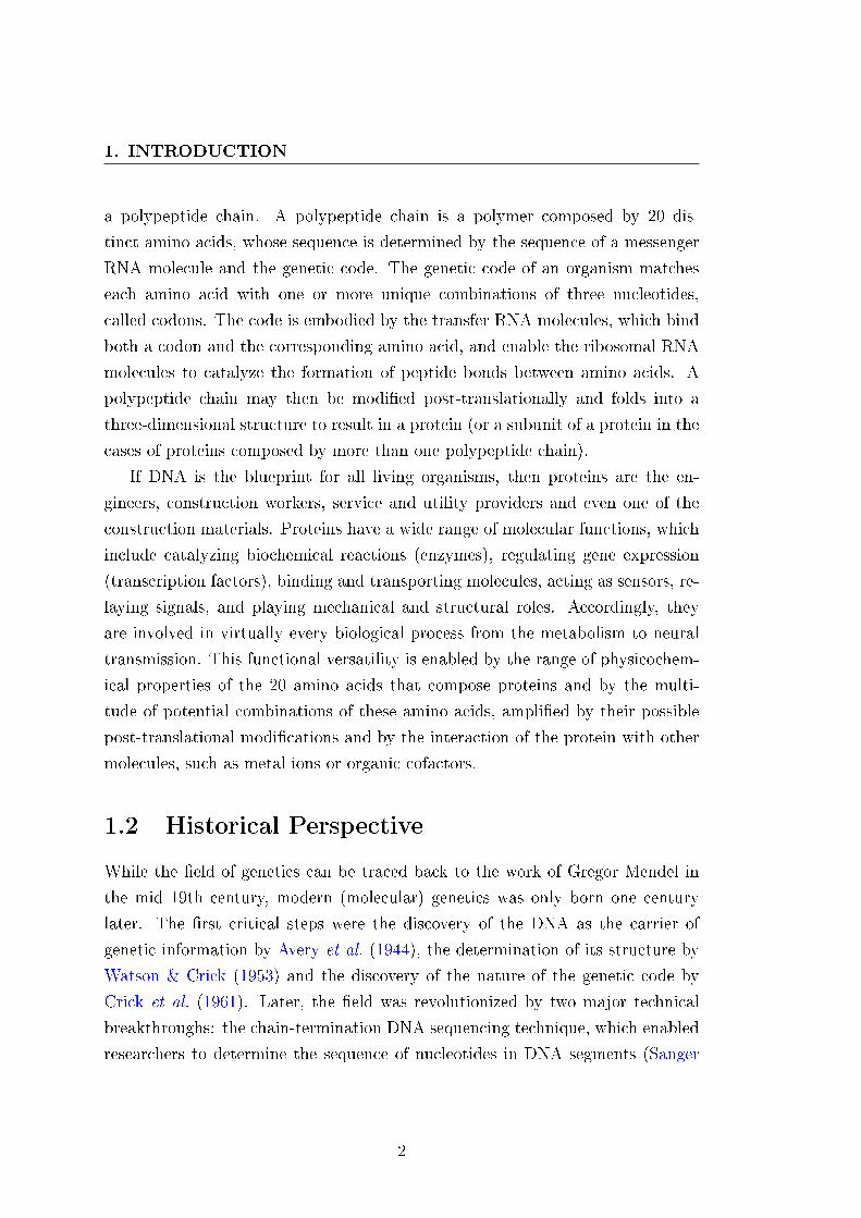
a polypeptide chain. A polypeptide chain is a polymer composed by 20 dis-
tinct amino acids, whose sequence is determined by the sequence of a messenger
RNA molecule and the genetic code. The genetic code of an organism matches
each amino acid with one or more unique combinations of three nucleotides,
called codons. The code is embodied by the transfer RNA molecules, which bind
both a codon and the corresponding amino acid, and enable the ribosomal RNA
molecules to catalyze the formation of peptide bonds between amino acids. A
polypeptide chain may then be modi�ed post-translationally and folds into a
three-dimensional structure to result in a protein (or a subunit of a protein in the
cases of proteins composed by more than one polypeptide chain).
If DNA is the blueprint for all living organisms, then proteins are the en-
gineers, construction workers, service and utility providers and even one of the
construction materials. Proteins have a wide range of molecular functions, which
include catalyzing biochemical reactions (enzymes), regulating gene expression
(transcription factors), binding and transporting molecules, acting as sensors, re-
laying signals, and playing mechanical and structural roles. Accordingly, they
are involved in virtually every biological process from the metabolism to neural
transmission. This functional versatility is enabled by the range of physicochem-
ical properties of the 20 amino acids that compose proteins and by the multi-
tude of potential combinations of these amino acids, ampli�ed by their possible
post-translational modi�cations and by the interaction of the protein with other
molecules, such as metal ions or organic cofactors.
1.2 Historical Perspective
While the �eld of genetics can be traced back to the work of Gregor Mendel in
the mid 19th century, modern (molecular) genetics was only born one century
later. The �rst critical steps were the discovery of the DNA as the carrier of
genetic information by Avery et al. (1944), the determination of its structure by
Watson & Crick (1953) and the discovery of the nature of the genetic code by
Crick et al. (1961). Later, the �eld was revolutionized by two major technical
breakthroughs: the chain-termination DNA sequencing technique, which enabled
researchers to determine the sequence of nucleotides in DNA segments (Sanger
2
1.2 Historical Perspective
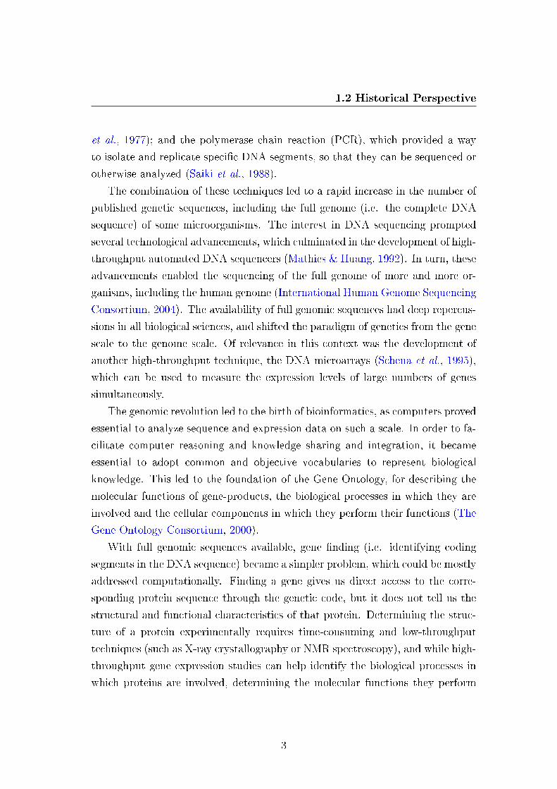
et al., 1977); and the polymerase chain reaction (PCR), which provided a way
to isolate and replicate speci�c DNA segments, so that they can be sequenced or
otherwise analyzed (Saiki et al., 1988).
The combination of these techniques led to a rapid increase in the number of
published genetic sequences, including the full genome (i.e. the complete DNA
sequence) of some microorganisms. The interest in DNA sequencing prompted
several technological advancements, which culminated in the development of high-
throughput automated DNA sequencers (Mathies & Huang, 1992). In turn, these
advancements enabled the sequencing of the full genome of more and more or-
ganisms, including the human genome (International Human Genome Sequencing
Consortium, 2004). The availability of full genomic sequences had deep repercus-
sions in all biological sciences, and shifted the paradigm of genetics from the gene
scale to the genome scale. Of relevance in this context was the development of
another high-throughput technique, the DNA microarrays (Schena et al., 1995),
which can be used to measure the expression levels of large numbers of genes
simultaneously.
The genomic revolution led to the birth of bioinformatics, as computers proved
essential to analyze sequence and expression data on such a scale. In order to fa-
cilitate computer reasoning and knowledge sharing and integration, it became
essential to adopt common and objective vocabularies to represent biological
knowledge. This led to the foundation of the Gene Ontology, for describing the
molecular functions of gene-products, the biological processes in which they are
involved and the cellular components in which they perform their functions (The
Gene Ontology Consortium, 2000).
With full genomic sequences available, gene �nding (i.e. identifying coding
segments in the DNA sequence) became a simpler problem, which could be mostly
addressed computationally. Finding a gene gives us direct access to the corre-
sponding protein sequence through the genetic code, but it does not tell us the
structural and functional characteristics of that protein. Determining the struc-
ture of a protein experimentally requires time-consuming and low-throughput
techniques (such as X-ray crystallography or NMR spectroscopy), and while high-
throughput gene expression studies can help identify the biological processes in
which proteins are involved, determining the molecular functions they perform
3
1. INTRODUCTION
also requires low-throughput assays. As these low-throughput experimental meth-
ods are unable to keep up with the rate at which new sequences are published,
the gap between sequence data and experimental functional knowledge contin-
ues to widen (Devos & Valencia, 2000; Friedberg, 2006). In order to bridge this
gap, researchers have adopted computational methods for function and structure
prediction.
1.3 Protein Function Prediction
The functions a protein can perform are deeply related to its structure (Fried-
berg, 2006), even if there are cases of readaptation of proteins throughout evo-
lution (Whisstock & Lesk, 2003). Likewise, the three-dimensional structure of a
protein is strongly conditioned by its sequence, even if there are factors such as
post-translational modi�cations to consider (Whisstock & Lesk, 2003). However,
the complexity of the minutial interactions involved in the protein folding pro-
cess make it extremely di�cult to model in silico (Zhang, 2008). Thus, de novo
sequence-based structure predictions require extensive computational resources
and generally have a low resolution (Zhang, 2008). Comparative modelling ap-
proaches, which use known structures as templates, are computationally lighter
and generally more accurate (Zhang, 2008), but the fact that only a minor frac-
tion of known proteins have experimentally determined structures severely limits
their applicability. Therefore, protein function prediction approaches typically
rely on sequence data alone.
One of the most common and simplest approaches for sequence-based protein
function prediction is the alignment-based inference. This approach consists of
employing a sequence alignment algorithm such as BLAST (Altschul et al., 1990)
to �nd proteins with similar sequence to the query protein. The function of the
query protein is then directly inferred from the functions of the proteins found,
in what is essentially a form of nearest neighbors classi�cation. The underlying
assumption behind this approach is that proteins that have similar sequences are
likely homologues (i.e. have evolved from a more or less recent common ancestor)
and can be expected to perform similar if not identical functions. Thus, the reli-
ability of this approach is directly dependent on the degree of sequence similarity
4

1.3 Protein Function Prediction
between the proteins (Tian & Skolnick, 2003). However, cases of divergent evolu-
tion (i.e. homologues that have signi�cantly di�erent functions) and convergent
evolution (i.e. unrelated proteins that perform the same function) are not un-
common, and make this approach error-prone and inherently limited (Whisstock
& Lesk, 2003). While it is considered reliable when the sequence alignments are
carefully analyzed and inferences are drawn from proteins with experimentally
determined functions, its pervasive and often incautious use has led to the ac-
cumulation of annotation errors in protein databases (Devos & Valencia, 2001;
Jones et al., 2007; Karp, 1998).
Another common approach to predict protein function is signature-based clas-
si�cation, wherein sequence signatures are extracted from families of functionally
related proteins, typically through multiple sequence alignment methods such
as hidden Markov models. New proteins are then classi�ed by searching for
known signatures and assigning the functional aspects associated with the signa-
tures found (Hunter et al., 2009; Whisstock & Lesk, 2003). Despite also being
based on sequence alignments, this approach is generally more robust than the
alignment-based inference, since it involves a more extensive comparison of pro-
tein sequences. However, it is also based on the assumption of homology, and
therefore may also be foiled by cases of divergent evolution. Like the alignment-
based inference, it is reliable when based on families of proteins with experimen-
tally determined functions, but less reliable when those families include proteins
with inferred functions (Whisstock & Lesk, 2003).
Machine learning approaches not based on sequence alignments have also been
applied to predict functional aspects of proteins, with support vector machines
(SVMs) being particularly prominent (Han et al., 2006). In these approaches a
machine learning classi�er is trained on a dataset of proteins with known func-
tion, then used to classify new proteins. The main advantage of these approaches
is that they model proteins based on their function rather than sequence, and
try to �nd common patterns in functionally-related proteins irrespective of their
sequence similarity (Han et al., 2006). However, their applicability is limited to
relatively small classi�cation problems, since training machine learning classi�ers
with millions of protein sequences for thousands of di�erent functions is simply
unfeasible. Another limitation shared by most machine learning methodologies
5
1. INTRODUCTION
is that they require data of �xed length, and therefore must convert protein
sequences into vectors of features (Han et al., 2006; Ong et al., 2007). The result-
ing loss of information makes these approaches less sensitive than the approaches
based on sequence alignments, and therefore less suitable for predicting detailed
functional aspects. Indeed, machine learning approaches have been mostly ap-
plied to predict generic functional aspects, such as whether proteins bind DNA
(Garg & Gupta, 2008; Han et al., 2006; Langlois et al., 2007; Liao et al., 2011).
Thus, in practice, machine learning approaches have been unable to compete with
sequence alignment approaches for general-purpose protein function prediction.
1.4 Thesis and Contributions
My thesis is that it is possible to extract su�cient information from protein
sequences to make reliable detailed function predictions without the use of se-
quence alignments, and therefore develop machine learning approaches that can
compete with alignment-based approaches for general-purpose protein function
prediction. To prove this thesis, I developed and/or evaluated multiple machine
learning approaches in the context of detailed function prediction. Additionally,
to understand the limits of protein function prediction, I studied the relationship
between functional similarity and sequence similarity and the issues that a�ect
the quality of the functional annotations of proteins. My work was developed
within the XLDB group of the LaSIGE research unit and included collaborations
with both XLDB colleagues and colleagues from other institutions.
The main contributions of my work are:
� The �rst large-scale evaluation of the use of semantic similarity approaches
to measure functional similarity between proteins based on their functional
annotations, including a detailed study of the relationship between func-
tional similarity and sequence similarity, presented in Chapter 3. This
evaluation highlighted the simGIC measure as the most suitable to mea-
sure functional similarity, and brought useful insights about the limits of
alignment-based protein function prediction.
6
1.4 Thesis and Contributions
� The �rst large-scale study assessing the quality and consistency of the
molecular function annotations of proteins that considers electronic an-
notations; plus a novel data mining algorithm, based on association rule
learning, to �nd implicit relationships between molecular function terms
with the goal of improving annotation consistency. Presented in Chapter 4,
this study shows that an estimated 20% of the proteins are inconsistently
annotated, which a�ects an estimated 88% of the protein functions. The
data mining algorithm I developed was able to �nd 1,101 implicit relation-
ships with an estimated precision of 83%, with a more selective version
having an estimated precision of 94% but �nding only 550 relationships.
� The development of the recently proposed Peptide Program methodology
(Falcao, 2005), designed to deal directly with protein sequences, and the
evaluation of this methodology in detailed enzyme classi�cation, presented
in Chapter 5. This evaluation showed that on datasets up to 1500 proteins,
Peptide Programs outperform both alignment-based inference classi�ers and
state of the art SVM classi�ers, but due to the complexity of the search
space, are unsuitable for larger classi�cation problems.
� The evaluation of the performance of multiple vector representations of
protein sequences in detailed enzyme classi�cation, including the novel lo-
cal amino acid composition representation, and the tripeptide composition
representation, which had been previously tested only in a few particular
applications (Jain et al., 2008; Mishra et al., 2007). In addition to test-
ing these representations with the SVM methodology, I developed a simple
Peptide Program framework for linear classi�cation based on vector rep-
resentations, called Vector Programs. Presented in Chapter 6, my evalu-
ation showed that the tripeptide composition representation was ideal for
detailed protein function prediction, as the SVMs based on this represen-
tation surpassed the precision of all other approaches tested. Furthermore,
the tripeptide composition representation was su�ciently informative to en-
able the direct comparison of protein sequences, with classi�cation results
that matched or surpassed those obtained with sequence alignments. The
7

1. INTRODUCTION
Vector Program methodology using the local amino acid composition repre-
sentation matched the Peptide Programs and surpassed all other approaches
tested on datasets up to 1500 proteins.
� The evaluation of the novel tripeptide-based measure of sequence similar-
ity, TripSim, in molecular function annotation prediction; plus the devel-
opment and evaluation of the hybrid TriGOPred prediction algorithm, that
combines a TripSim search with SVM classi�ers based on the tripeptide
composition representation. As presented in Chapter 7, this evaluation
was based on the most generic formulation of the prediction problem, con-
sisting on predicting the full molecular function annotations of each test
protein by comparison with all proteins of known function. This evaluation
demonstrated that the TripSim measure is a viable alternative to BLAST
in the context of function prediction, as it led to identical or slightly supe-
rior prediction results when using the same prediction algorithms used with
BLAST. Considering that TripSim is computationally simpler and faster
than BLAST, its adoption can speed up similarity searches and function
predictions. Additionally, the TriGOPred algorithm was also established as
a good alternative to the traditional nearest-neighbors approaches, as it led
to identical prediction results within a competitive prediction time. Consid-
ering that TriGOPred predictions are based on a larger number of proteins
than typical nearest-neighbors predictions, they should be in principle less
a�ected by annotation errors and less prone to propagate them.
8
Chapter 2
State of the Art
2.1 About Proteins
Proteins are composed by one or more polypeptide chains, typically folded
into a globular or �brous three-dimensional structure. A polypeptide chain
is a polymer of amino acids, synthesized from a messenger RNA template,
which in turn is synthesized from a DNA template gene. All protein-forming
amino acids are α amino acids, having the generic formula H2NCHRCOOH,
where R is an organic substituent called the side-chain. In a polypeptide,
amino acids are linked by peptide bonds, in which the carboxyl group (-
COOH) of one amino acid combines with the amino group (H2N-) of the
other amino acid to form an amide (-C(O)NH-). Thus, a polypeptide is a
linear polymer with a continuous backbone of amino acid residues of the
form -HNCHRC(O)-, which does not involve the side-chains directly.
2.1.1 Amino Acids
There are twenty standard protein-forming amino acids encoded by the
genetic code of all organisms: alanine (A), arginine (R), asparagine (N),
aspartic acid (D), cysteine (C), glutamine (Q), glutamic acid (E), glycine
(G), hystidine (H), isoleucine (I), leucine (L), lysine (K), methionine (M),
9
2. STATE OF THE ART
phenylalanine (F), proline (P), serine (S), threonine (T), tryptophan (W),
tyrosine (Y) and valine (V). There is a rarer twenty-�rst amino acid, se-
lenocystein (U), which occurs in some enzymes and is translated from the
codon UGA (which is normally a stop codon) in the presence of certain
secondary structures of the messenger RNA. A twenty-second amino acid,
pyrrolysine (O), is encoded by some archaea with the codon UAG, which in
other organisms is also a stop codon. The post-translational modi�cation of
the protein-forming amino acids leads to additional amino acids that occur
in proteins (such as hypusine), but these are not encoded by the genetic
code.
2.1.2 Sequence
The primary structure of proteins corresponds to the sequence of amino
acids in the polypeptide chain(s). Protein sequences are typically repre-
sented as strings, with each of the twenty-two amino acids being represented
by their single letter code. This representation enables protein sequences
to be compared through sequence alignments, but does not cover post-
translational modi�cations. Protein sequences range in length from as few
as 40 to several thousand amino acids (polypeptides with less than 40 amino
acids exist but are typically called peptides rather than proteins).
2.1.3 Three-Dimensional Structure
The secondary structure of proteins corresponds to the three-dimensional
form of local segments of the protein, as determined by the hydrogen bonds
between the amino acids and/or by the backbone angles. The tertiary
structure corresponds to the three-dimensional structure into which a single
polypeptide chain folds, as determined by non-speci�c hydrophobic inter-
actions (i.e. the burial of hydrophobic residues to avoid exposure to water)
and speci�c tertiary interactions (e.g. salt bridges, hydrogen bonds, and
disul�de bonds). In multimeric proteins, the quaternary structure corre-
sponds to the assembly of two or more polypeptide chains (called subunits)
10

2.1 About Proteins
to form a complex (or multimer) which is stabilized by the same interactions
that determine the tertiary structure.
Secondary structures are typically represented in string form, with each
amino acid being assigned a single letter corresponding to the type of sec-
ondary structure it forms. Tertiary and quaternary structures are repre-
sented by the spacial coordinates of the atoms that compose each amino
acid in the protein, which enables structures to be compaired through struc-
tural alignments.
2.1.4 Function
Unlike the sequence and the three-dimensional structure, the function of a
protein is hard to de�ne or describe objectively. Proteins perform functions
at the molecular level which range from structural roles to the catalysis of
biochemical reactions (proteins with catalytic functions are called enzymes).
These molecular functions take place in certain cellular components (e.g.
the cell membrane), in certain cells or regions of an organism (e.g. neurons
in the brain) and are integrated into certain biological processes (e.g. neuro-
transmission). The expression and activity of a protein is regulated by the
cell and organism, and is a�ected by factors such as the activities of other
proteins or the concentrations of chemical substances. Since protein func-
tions only exist as an integral part of living systems, any de�nition of protein
function is necessarily an abstraction, and any description of the function
of a protein is necessarily incomplete. Yet, describing protein functions as
objectively and completely as possible is critical to enable computer rea-
soning, knowledge sharing and reliable protein function predictions. Thus,
the traditional free-text functional descriptions are giving way to structured
and formal functional representations.
11

2. STATE OF THE ART
2.2 Protein Resources
2.2.1 The UniProt Knowledge Base
The UniProt Knowledge Base (UniProtKB) is a comprehensive database of
protein sequences and functional information founded in 2003, as the result
of a pooling of resources of the European Bioinformatics Institute (EBI),
the Swiss Institute of Bioinformatics (SIB), and the Protein Information
Resource (PIR) (Apweiler et al., 2004). The UniProtKB consists of two
sections: the Swiss-Prot, which contains high-quality entries reviewed by
expert curators and manually annotated, and the TrEMBL, containing un-
reviewed, automatically annotated entries (The UniProt Consortium, 2010).
The Swiss-Prot currently includes over half a million proteins, whereas the
TrEMBL includes almost twenty million. However, the majority of the pro-
teins in TrEMBL are derived from the translation of gene sequences sub-
mitted to public nucleic acid databases, and their existence has not been
veri�ed. 97% of the TrEMBL proteins have either a predicted existence or
an existence inferred from homology, less than 3% have been identi�ed at
the transcript level (in DNA microarray studies) and only 0.07% have been
veri�ed at the protein level.
The UniProtKB has become a central hub for protein research, as in addi-
tion to storing information about the sequence and function of the protein,
each UniProtKB entry includes extensive cross-references to other databases
that have information about the protein (such as its three-dimensional
structure or the sequence pro�les to which it belongs). Conversely, most
other databases have adopted UniProtKB accession numbers as identi�ers
for proteins, and cross-reference UniProtKB entries.
2.2.2 The Worldwide Protein Data Bank
The Worldwide Protein Data Bank (wwPDB) is a comprehensive database
of three-dimensional structures of proteins which resulted from the integra-
tion of the structural databases of the United States (RCSB PDB), Europe
12
2.2 Protein Resources
(PDBe) and Japan (PDBj) (Berman et al., 2003). The wwPBD stores
only experimentally determined protein structures, the large majority of
which are determined by X-ray crystallography or NMR spectroscopy. The
wwPDB includes approximately 80,000 structures, and some of these are
redundant, so they represent only a minor fraction of UniProtKB proteins.
2.2.3 The Enzyme Commission System
Dating back to 1961, the Enzyme Commission (EC) system was the �rst at-
tempt to describe protein functions objectively, albeit restricted to enzymes
(Webb, 1992). The EC system classi�es enzymes hierarchically according
to the reactions they catalyze, independently of their sequence or structural
similarities. The EC hierarchy has four levels, represented by four digits in
the EC code (e.g. EC 1.1.1.1). The �rst digit represents the enzyme class,
which can be one of the following six generic categories: EC 1 - Oxidoreduc-
tase; EC 2 - Transferase; EC 3 - Hydrolase; EC 4 - Lyase; EC 5 - Isomerase;
EC 6 - Ligase. The second digit represents the subclass, which generally
describes the type of substrate or chemical bond that the enzyme acts upon.
The third digit represents the sub-subclass, which has a variable meaning
from class to class. The fourth digit represents the enzyme family, which
corresponds to a single enzymatic reaction (e.g. EC 1.9.3.1 - cytochrome-c
oxidase) or a family of enzymatic reactions with related substrates (e.g. EC
1.1.1.1 - alcohol dehydrogenase).
The annotation of UniProtKB proteins with EC codes is maintained by
the ENZYME database (Bairoch, 2000), although the BRENDA database
contains more comprehensive information about the EC families and their
corresponding enzymes (Scheer et al., 2011).
While the EC system provides a structured representation of enzyme func-
tions, the information in EC entries is available only in human-readable
form, and not readily accessible for computation. For instance, the reac-
tion catalyzed by a given EC family is described with a chemical equation,
13
2. STATE OF THE ART
so accessing this information computationally would require parsing the
equation and processing the chemical formulas.
2.2.4 The Gene Ontology
Founded in 1998, the Gene Ontology (GO) was a coordinated e�ort to unify
the descriptions of gene and protein functions across all species, since at the
time each species-speci�c database used its own terminology (The Gene On-
tology Consortium, 2000). More than a simple terminology, GO sought to
represent functional knowledge in a structured and formal way, beyond even
the EC system. GO comprises three integrated ontologies, corresponding to
the aspects molecular function, biological process and cellular component.
Each of these ontologies is structured as directed acyclic graph, which is
similar to a hierarchy but enables multi-parenting. Within each ontology,
the terms (or nodes) may be linked by parent-child relationships (is a),
part-whole relationships (part of, has part) or regulatory relationships (reg-
ulates, positively regulates, negatively regulates). While initially the three
GO ontologies were considered orthogonal, currently molecular functions
can be part of biological processes, and there are plans to introduce the
occurs in relationship, which will link molecular functions and biological
processes to cellular components (The Gene Ontology Consortium, 2012).
While more structured and formal than the EC system, GO is also lacking
in accessibility for computation, since GO term de�nitions are unstructured
textual de�nitions. However, GO is being normalized and extended with
computable logical de�nitions, including references to external ontologies,
which will greatly facilitate computer reasoning (Mungall et al., 2011).
Of the three GO ontologies, the molecular function is the most relevant
for protein function prediction, since it is the most di�cult aspect to de-
termine experimentally on large scale studies. The two major branches of
the molecular function ontology are the catalytic activity branch, which
describes enzyme functions and is largely based on the structure of the EC
system, and the binding branch, which describes interactions with other
14
2.2 Protein Resources
molecules (from metal ions to nucleic acids and other proteins). Together,
these two branches account for over 80% of the molecular function terms.
GO is currently the de facto standard for the functional annotation of pro-
teins. Some GO annotations are maintained and curated by GO itself, but
the Gene Ontology Annotation (GOA) database is the responsible for an-
notating UniProtKB proteins (Barrell et al., 2009). GO annotations are
tagged with evidence codes which indicate the type of evidence upon which
the annotation was based. These range from the most reliable �inferred from
direct assay� (IDA) to the least reliable �inferred from electronic annotation�
(IEA), with the latter accounting for over 98% of the GOA annotations (as
of the GOA release of October 2010).
2.2.5 The InterPro
The InterPro is an integrated database of protein families, domains and
functional sites (generically called signatures) which are typically obtained
from multiple sequence alignment methods such as hidden Markov models
(Hunter et al., 2009). The InterPro combines signature information from
several member databases, such as PROSITE (Hulo et al., 2006) and Pfam
(Finn et al., 2008). InterPro signatures can be manually or automatically
extracted, and range from local motifs and �ngerprints to global sequence
domains and structural folds. The goal of the InterPro is to identify features
in known proteins which can be applied to functionally characterize new
protein sequences. InterPro includes cross-references to GO, and is the
main source of IEA molecular function annotations, accounting for over 70%
of the molecular function annotations in GOA. The main limitation of the
InterPro is the lack of information about the reliability of the signatures. For
instance, signatures based on experimental evidence or detailed structural
analysis are more reliable than signatures based only on multiple sequence
alignments, but this information is not readily available in InterPro.
15
2. STATE OF THE ART
2.3 Alignment-Based Protein Function Predic-
tion
Given that for the majority of the published protein sequences there is
no information available other than the sequence itself and the organism
from which it came, protein function prediction often relies exclusively on
sequence data. Sequence alignments enable protein sequences to be com-
pared and analyzed, and have been on the basis of protein function pre-
diction since the beginning of the genomic era (Devos & Valencia, 2000).
BLAST (Altschul et al., 1990) and the more sensitive PSI-BLAST (Altschul
et al., 1997) have been the most popular algorithms for pairwise sequence
alignments, mostly thanks to their speed, since they are not guaranteed to
�nd the optimum alignment. Yet, being able to compare a new protein
sequence to each of the 12 million UniProtKB proteins in a few minutes
is an unparalleled advantage. Hidden Markov models (HMMs) (Hughey &
Krogh, 1996) have been the most prominent method for multiple sequence
alignments, surpassing iterative pairwise approaches both in speed and sen-
sitivity (Söding, 2005).
2.3.1 Alignment-Based Inference
Alignment-based inference consists of employing a pairwise sequence align-
ment algorithm (typically BLAST or PSI-BLAST) to �nd proteins with
similar sequence to the query protein, then inferring the function of the
query protein based on the functions of the proteins found. The prediction
can be done through manual analysis of the sequence alignments, or auto-
matically, typically employing a nearest neighbors classi�cation approach.
From a biological perspective, this approach is based on the assumption
that similar sequences have evolved from a common ancestor (i.e. are ho-
mologues) and therefore should perform at least similar functions (Devos &
Valencia, 2000). The problem with this assumption is that cases of divergent
evolution are not uncommon, and throughout evolutionary history proteins
16
2.3 Alignment-Based Protein Function Prediction
have sometimes been adapted to perform dramatically di�erent functions
while retaining high sequence similarity (Whisstock & Lesk, 2003). While
increasing the similarity threshold reduces the number of false predictions
(or type I errors) it also reduces the number of true predictions (thus in-
creasing the number of type II errors) (Tian & Skolnick, 2003). Conversely,
there are proteins that are only distantly related (i.e. remote homologues)
but still perform similar or identical functions (Whisstock & Lesk, 2003).
While the more sensitive PSI-BLAST algorithm (Altschul et al., 1997) can
capture some of these remote homologues, this comes at the expense of
making more false predictions.
The reliability of this approach also depends on the way predictions are
made. Manual predictions, based on carefully analyzed sequence align-
ments and on proteins with experimentally determined functions are gen-
erally considered reliable, and even more so when based on closely related
organisms and taking into consideration the phylogeny and the genomic
context (Pellegrini et al., 1999). On the other hand, automatic predictions
based on a few nearest-neighbors with no criterion other than sequence sim-
ilarity are evidently less reliable (Devos & Valencia, 2001). Unfortunately,
the distinction between experimentally determined and inferred functional
annotations in protein databases was not always clear, and combined with
the pervasive and often incautious use of alignment-based inferences, this
led to the propagation of annotation errors (Devos & Valencia, 2001; Jones
et al., 2007; Karp, 1998).
There are several issues that automated alignment-based inference applica-
tions must address to improve their reliability. First, they must ensure the
global quality of the sequence alignments, since local alignment algorithms
such as BLAST can return signi�cant yet partial alignments. Making infer-
ences based on partial alignments increases the risk of prediction errors, as
the aligned segments may not be directly related to the function of the pro-
teins, or may correspond to only one aspect of that function (e.g. a cofactor
binding region). Second, when making and scoring predictions, they must
take into account not only the number and sequence similarity of the aligned
17

2. STATE OF THE ART
proteins, but also the reliability of their functional annotations. Predictions
based on proteins with inferred annotations should be avoided or at least
given a lower con�dence score than predictions based on proteins with ex-
perimentally determined annotations. Third, they must be able to reason
within the protein function space, so as to be able to generalize and predict
generic functional aspects when detailed aspects are unsuitable. Existing
protein function prediction applications that meet these criteria include
GOtcha (Martin et al., 2004), Blast2GO (Conesa et al., 2005) and PFP
(Hawkins et al., 2009).
2.3.2 Signature-Based Classi�cation
Signature-based classi�cation relies on identifying sequence signatures from
families of functionally related proteins through multiple sequence align-
ment methods (typically HMMs). These signatures can then be used to
analyze and classify new protein sequences (Hunter et al., 2009; Whisstock
& Lesk, 2003). Signatures range from local sequence motifs to global se-
quence domains, can be manually curated or obtained automatically, and
can be based on experimental or structural information in addition to the
sequence. From a machine learning perspective, this approach is also a form
of nearest-neighbors classi�cation, although it is based on protein clusters
rather than on individual proteins. Thus, it is generally more robust and
less prone to propagate errors than the alignment-based inference approach,
since classi�cation typically involves a more extensive comparison of pro-
tein sequences. Furthermore, it is more reliable than the alignment-based
inference for lower sequence similarity levels, since HMMs are more sensitive
than PSI-BLAST (Söding, 2005). However, it must be noted that signature-
based classi�cation is also largely based on the assumption that homologous
proteins perform similar functions, and as such may also be compromised
by cases of divergent evolution. Thus, its reliability is directly dependent on
the quality of the signatures themselves, with manually curated signatures
with supporting experimental evidence being the most reliable, and auto-
matically obtained signatures the least reliable (Whisstock & Lesk, 2003).
18

2.4 Machine Learning Approaches for Protein Function Prediction
Signature-based classi�cation is centered on the InterPro and its member
databases (Hunter et al., 2009), which are the main source of molecular
function annotations of UniProtKB proteins. The InterProScan webtool
allows researchers to analyze new sequences in search of known InterPro
signatures and use those signatures to predict the function of the sequences.
By integrating signatures from multiple databases, and based on multiple
di�erent approaches, the InterPro increases the reliability of function pre-
dictions (Friedberg, 2006; Whisstock & Lesk, 2003).
2.4 Machine Learning Approaches for Protein
Function Prediction
While less popular than alignment-based approaches, machine learning ap-
proaches not based on sequence alignments have also been applied with
some success to particular protein function prediction problems (Han et al.,
2006). Generically, these approaches consist in training a machine learn-
ing classi�er on a dataset of proteins with known function, then using that
classi�er to predict the function of new protein sequences. They di�er from
alignment-based approaches in that they model proteins based on their func-
tion rather than their sequence. As such, they can �nd common patterns
in functionally-related proteins even when their sequence similarity is low
(Han et al., 2006). Furthermore, the machine learning methodologies used
in this context are generally more so�sticated and more robust than the
nearest neighbors classi�cation used in alignment-based approaches. How-
ever, they are also computationally more intensive, so their applicability
is limited to relatively small classi�cation problems (up to the scale of the
tens of thousands of proteins). Thus, overall, these approaches have been
unable to compete with alignment-based approaches for general-purpose
protein function prediction.
19

2. STATE OF THE ART
2.4.1 Support Vector Machines
Several machine learning methodologies have been tested in protein func-
tion prediction problems, including decision trees (Langlois et al., 2007;
Yang et al., 2007), arti�cial neural networks (ANNs) (Dubchak et al., 1995;
Pasquier et al., 2001; Yang & Hamer, 2007), inductive logic programming
(ILP) (King et al., 2000), and Support Vector Machines (SVMs) (Al-Shahib
et al., 2007; Bhardwaj et al., 2005; Cai et al., 2004; Han et al., 2004; Kumar
et al., 2007; Lin et al., 2006). However, SVMs have been by far the most pop-
ular methodology used in this context, overshadowing other methodologies
(Ben-Hur & Weston, 2008; Han et al., 2006; Ong et al., 2007). An SVM is a
non-probabilistic maximum margin binary classi�er, that maps data points
into a high-dimensional space using a kernel function, in order to separate
them linearly. SVMs are interesting for protein function prediction because
they deal better with data with a high number of attributes than most
other machine learning methodologies (Ben-Hur & Weston, 2008). The fact
that they are limited to binary classi�cation problems is not a signi�cant
drawback, since the protein function space is too complex to model in full
(it contains thousands of functions, ranging from completely unrelated to
near-identical). Thus, except for nearest neighbors approaches, all machine
learning methodologies must reduce the protein function prediction problem
to smaller classi�cation problems, be they binary or multiclass. Further-
more, binary classi�ers can be combined to produce multiclass classi�cation
(Saraç et al., 2010). As such, it is unclear whether multiclass classi�cation
algorithms have any practical advantage over binary classi�ction algorithms
in this context. However, it is worth mentioning the recent development of
structured-output SVMs for multiclass classi�cation (Sokolov & Ben-Hur,
2010).
2.4.2 Sequence Representations
Most machine learning methodologies (SVMs included) require data with a
�xed number of attributes. However, protein sequences in a given classi�ca-
20
2.4 Machine Learning Approaches for Protein Function Prediction
tion problem seldom have all the same length, or even matching segments
of the same length. Furthermore, the individual positions in a sequence
have no inherent meaning, since even closely related proteins can have in-
sertions and deletions that shift the sequence. This means that protein
sequences cannot be used directly with most machine learning methodolo-
gies, but rather must be converted into vectors of sequence-derived features
(Han et al., 2006; Ong et al., 2007). Finding suitable sets of descriptors to
represent protein sequences has been an important topic of research in this
�eld, with the focus being on capturing information about the order of the
amino acids in the sequence (Han et al., 2006; Ong et al., 2007). Proposed
representations have included simple descriptor sets based on the sequence
alone, such as the amino acid composition (Han et al., 2006) or the compo-
sition of pairs and trios of amino acids (dipeptides and tripeptides) (Jain
et al., 2008; Mishra et al., 2007), and more complex descriptor sets based
on physicochemical properties of the amino acids, such as the pseudo-amino
acid composition (Chou, 2001), the MoreauBroto autocorrelation (Feng &
Zhang, 2000), or the popular descriptor set of composition, transition and
distribution (Al-Shahib et al., 2007; Cai et al., 2004; Dubchak et al., 1995;
Han et al., 2004; Kumar et al., 2007; Lin et al., 2006).
Converting sequences into vectors of features inevitably leads to a loss of
information, which can make machine learning approaches less sensitive
than alignment-based approaches, and therefore less suitable for predicting
detailed functional aspects. Indeed, the vast majority of studies where ma-
chine learning approaches have been applied focused on predicting generic
functional aspects, such as whether proteins bind DNA or whether they
belong to a given EC class or subclass (Garg & Gupta, 2008; Kumar et al.,
2007; Langlois et al., 2007; Liao et al., 2011). Furthermore, the only exten-
sive study comparing the performance of multiple representations of protein
sequences was also evaluated on generic classi�cation problems (Ong et al.,
2007). Thus, it is unclear whether machine learning approaches can ac-
tually compete with alignment-based approaches when predicting detailed
functional aspects.
21
2. STATE OF THE ART
2.4.3 Application Issues
Since it is unfeasible to train a machine learning classi�er with the several
million known proteins, applying machine learning approaches to protein
function prediction requires selecting a representative set of proteins for the
particular classi�cation problem. Concretely, in the most common case of
binary classi�cation, it is necessary to select a set of positive instances (i.e.
proteins that have the functional aspect of interest) and a set of negative
instances (i.e. proteins that do not have that functional aspect). However,
the number of proteins that do not have any given functional aspect is
generally much greater than the number of proteins that do. On one hand,
a training set that respects the true proportion of positives and negatives
would be highly unbalanced, which could compromise the training and lead
to a biased classi�er (Akbani et al., 2004). On the other hand, reducing
the number of negatives to obtain a balanced training set can reduce the
accuracy of the classi�er, if the negative training set doesn't represent the
variety of existing negative proteins.
Another issue in the application of machine learning approaches to protein
function prediction is that it is di�cult to determine that a protein is truly
a negative for a given function, even if it has an experimentally determined
function. The reason for this is that few proteins have been studied to the
extent that all possible functions have been excluded. There are known
cases of proteins that perform multiple unrelated functions, such as the
enzyme phosphoglucose isomerase which also plays a role as a neural growth
factor and in cell signaling (Je�ery, 1999). Thus, it is possible that less
thoroughly studied proteins have unidenti�ed additional functions. The
existence of mislabeled negative instances could compromise classi�cation
accuracy (Brodley & Friedl, 1999).
22
Chapter 3
Measuring Functional Similarity
Between Proteins
3.1 Background
Comparing proteins at the functional level is essential to assess the qual-
ity of function predictions. Furthermore, studying the relationship between
sequence similarity and functional similarity can contribute to our under-
standing of the limits of sequence-based protein function prediction. Unlike
protein sequences or structures, there is no evident way to measure simi-
larity between protein functions, because functions lack measurable prop-
erties or an inherent objective representation. However, the wide adoption
of the Gene Ontology (GO) for functional annotation of proteins o�ers the
possibility of comparing protein functions by comparing their annotations,
through the use of semantic similarity measures.
There are two main approaches to measure semantic similarity between
terms of an ontology structured as a directed acyclic graph such as GO:
edge-based approaches, that use the edges (i.e. the relationships between
the terms) and their types as the main data source; and node-based ap-
proaches, where the nodes (i.e. the terms) and their properties are the
main data source. Edge-based approaches are mostly based on counting
23
3. MEASURING FUNCTIONAL SIMILARITY BETWEENPROTEINS
the number of edges in the path between two terms. While intuitive, the
assumptions upon which they are based are not true for GO, as nodes
and edges are not uniformly distributed in GO and two edges at the same
level in GO may correspond to di�erent semantic distances between terms.
Node-based approaches rely on comparing the properties of the terms in-
volved, which can be related to the terms themselves, their ancestors or
their descendants. One concept commonly used in these approaches, is the
information content (IC), which measures term speci�city and informative-
ness and is given by the negative log likelihood of annotation of a term.
Approaches based on the IC are less sensitive to the issues of variable se-
mantic distance and variable node density than edge-based measures, and
therefore are more suitable for comparing GO terms.
Applying semantic similarity measures to compare protein functions is not
trivial, since protein functions are typically described by several GO molecu-
lar function terms. As traditional semantic similarity measures are intended
to compare single terms, their application to proteins requires a strategy to
combine the semantic similarities of all their terms. Alternatively, a graph
comparison measure can be used directly to compute semantic similarity
between proteins, since the set of GO molecular function terms to which a
protein is annotated is essentially a subgraph of molecular function.
While semantic similarity measures had been proposed to compare protein
functions based on their GO annotations (Couto et al., 2007; Lord et al.,
2003; Schlicker et al., 2006), they had not been evaluated on large datasets.
In this chapter, I evaluate existing semantic similarity measures on a large
scale and study the relationship between sequence similarity and functional
(semantic) similarity.
24
3.2 Methods
3.2 Methods
3.2.1 Dataset
This study was based on the integrated ProteInOn database (Faria et al.,
2007), which combines protein data from the UniProtKB, term data from
GO and annotation data from GOA, as of the respective releases of February
2007.
The probability of annotation of each term was estimated from its frequency
of annotation in GOA, and then used to calculate the IC as described by
Resnik (1999). An alternative (non-electronic) IC was calculated consid-
ering only non-electronic annotations (i.e. not counting annotations with
evidence codes IEA, NAS, NA and NR). Both ICs were uniformized to
obtain a value in a 0-1 scale.
A dataset of 22,067 Swiss-Prot proteins was selected from the database,
consisting of proteins annotated to at least one GO molecular function
term of IC 65% or higher. This criterion ensures that poorly annotated
proteins (i.e. those with only very generic terms) are discarded, as they
would otherwise bias the semantic similarity results. The value of 65% was
chosen as a compromise between computational time and representativity
of the dataset, as a lower cut-o� would likely be su�cient to exclude most
of the poorly annotated proteins, but would also result in a larger dataset.
An all-against-all BLAST search was performed with a threshold e-value of
10-4, resulting in a �nal (full) dataset of 618,146 protein pairs.
To evaluate the in�uence of electronic annotations, a second dataset of
4,608 proteins was selected using the above criteria, but discarding proteins
annotated with electronic annotations, which lead to a �nal (non-electronic)
dataset of 49,480 protein pairs.
25

3. MEASURING FUNCTIONAL SIMILARITY BETWEENPROTEINS
3.2.2 Sequence Similarity Measures
To have results comparable to those obtained by Lord et al. (2003), I opted
for using the same measure of sequence similarity: the logarithm of the
BLAST score, averaging the BLAST scores in both directions (i.e. A against
B and B against A) to produce the log reciprocal BLAST score (LRBS):
LRBS(A,B) = log10
(BLASTscore(A,B) +BLASTscore(B,A)
2
)(3.1)
The issue of using LRBS as a similarity measure is that it is biased by the
length of the proteins. A poor alignment between two very long proteins can
have a higher score than a good alignment between two very short proteins.
Thus, I wanted to have an alternative measure of sequence similarity that
was independent of sequence length. Using the sequence identity was not
a viable alternative, because BLAST is a local alignment algorithm and
the sequence identity it returns is relative to the aligned segment rather
than the full protein. Thus, a partial alignment without mismatches will
have a higher sequence identity than a full sequence alignment with a single
mismatch. Thus, I conceived the relative reciprocal BLAST score (RRBS)
which is analogous to the sequence identity, but accounts for the full length
of the proteins and also for amino acid substitutions. Given two proteins,
RRBS is given by the sum of their reciprocal BLAST scores divided by the
sum of their self-BLAST scores:
RRBS(A,B) =BLASTscore(A,B) +BLASTscore(B,A)
BLASTscore(A,A) +BLASTscore(B,B)(3.2)
3.2.3 Semantic Similarity Measures
I tested a total of fourteen approaches to compute semantic similarity be-
tween proteins. I tested the three established term similarity measures pro-
posed by Resnik (1999), Lin (1998), and Jiang & Conrath (1997) using three
26

3.2 Methods
distinct combination strategies: Average (AVG), Maximum (MAX), Best-
Match Average (BMA) (Schlicker et al., 2006). For each of these three mea-
sures, I tested also the GraSM variant proposed by Couto et al. (2007), but
only with the BMA combination strategy. Finally, I tested two graph-based
measures: simUI (Gentleman, 2005) and the newly developed simGIC.
Given two terms c1 and c2 and their most informative common ancestor cA,
Resnik's measure is given by:
simRes(c1, c2) = IC(cA) (3.3)
Lin's measure is given by:
simLin(c1, c2) =2× IC(cA)
IC(c1) + IC(c2)(3.4)
and Jiang and Conrath's similarity measure (derived from the distance mea-
sure as suggested by the authors) is given by:
simJC(c1, c2) = 1 + IC(cA)−(IC(c1) + IC(c2))
2(3.5)
The GraSM variant consists of using the average IC of all disjoint common
ancestors instead of only that of the most informative (Couto et al., 2007).
Semantic similarity between proteins was calculated from the term similar-
ity measures using the combination approaches previously mentioned. For
each protein, the set of its direct annotations was obtained, and redundant
annotations (i.e. those already implied by a more speci�c annotation) were
excluded. Given two proteins A and B, with non-redundant sets of GO
terms GO(A) and GO(B) respectively: the maximum approach is given by
the maximum of the similarity between each term in GO(A) and each term
in GO(B); the average approach is given by the average similarity between
each combination of terms in GO(A) and GO(B); and the best-match aver-
age approach is given by the average similarity between each term in GO(A)
and its most similar term in GO(B) and vice-versa.
27
3. MEASURING FUNCTIONAL SIMILARITY BETWEENPROTEINS
Additionally, semantic similarity between proteins was also calculated di-
rectly using the graph-based measures simUI and simGIC. In the case of
these measures, the extended set of annotations is obtained for each pro-
tein, consisting of the direct annotations and all their ancestral terms up
to the root node. Given two proteins A and B, with extended sets of GO
term annotations GO'(A) and GO'(B) respectively, simUI is given by the
Jaccard index between the two sets:
simUI(A,B) =|GO′(A) ∩GO′(B)||GO′(A) ∪GO′(B)|
(3.6)
whereas simGIC is given by the weighted Jaccard index between the two
sets, with each term being weighted by its IC:
simGIC(A,B) =
∑t∈GO′(A)∩GO′(B) IC(t)∑t∈GO′(A)∪GO′(B) IC(t)
(3.7)
3.2.4 Data Processing and Modelling
The raw semantic similarity versus sequence similarity results consist of too
many scattered data points to discern a pattern or establish any term of
comparison between measures. This is expected since cases of functionally
similar proteins with unrelated sequences, and vice-versa, are well known
to occur. To study the relationship between semantic similarity and se-
quence similarity I computed average semantic similarity values for discrete
sequence similarity intervals for each of the sequence similarity metrics. Se-
quence similarity intervals were selected by number of data points, in order
to ensure that all intervals are equally representative. In the full dataset
each interval contains 5,000 points, whereas in the non-electronic dataset
each interval contains 1,000 points. For each interval the average values of
sequence and semantic similarity were computed. The semantic similarity
standard deviation per interval was around 20%.
28

3.3 The Relationship Between Functional Similarity and SequenceSimilarity
The behaviour of the average semantic similarity versus sequence similarity
values was modelled by non-linear regression using the least squares method
and the Newton optimization algorithm.
3.3 The Relationship Between Functional Sim-
ilarity and Sequence Similarity
3.3.1 Modelling
Upon observing the behaviour of the averaged semantic similarity results
(Figures 3.1 and 3.2), it was clear that the relationship between functional
semantic similarity and sequence similarity was not linear, regardless of
dataset, sequence similarity measure or semantic similarity measure. What
is more, within each dataset and sequence similarity measure, the majority
of the semantic similarity measures were similar in behaviour.
In order to quantify the di�erences between the measures, and to study
the properties of the relationship between functional (semantic) similarity
and sequence similarity, I needed to �nd functions that could model the
behaviour of the results. I found that normal cumulative distribution func-
tions (NCDF ) were able to suitably model the overall behaviour of the results
for most of the semantic similarity measures, and additionally, the in�uence
of the NCDF parameters in the shape of the resulting curve is intuitive. Ini-
tially the results were modelled by a single NCDF , using a translation factor
a to account for the fact that the minimum (averaged) semantic similarity
values were greater than zero and a scale factor b to account for the range
of the semantic similarity values being smaller than 1:
simfunction = a+ b×NCDF (simsequence, µ, σ) (3.8)
However, I found that for the full dataset, a single NCDF could not suitably
describe all the aspects of the behaviour of the data, namely the evident
bimodal-like behaviour, i.e the fact that there are two distinct zones where
29
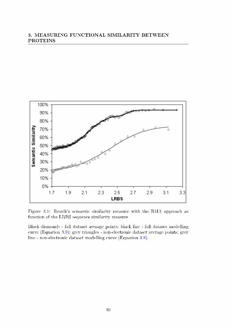
3. MEASURING FUNCTIONAL SIMILARITY BETWEENPROTEINS
Figure 3.1: Resnik's semantic similarity measure with the BMA approach asfunction of the LRBS sequence similarity measure
Black diamonds - full dataset average points; black line - full dataset modellingcurve (Equation 3.9); grey triangles - non-electronic dataset average points; greyline - non-electronic dataset modelling curve (Equation 3.8).
30

3.3 The Relationship Between Functional Similarity and SequenceSimilarity
Figure 3.2: Resnik's semantic similarity measure with the BMA approach asfunction of the RRBS sequence similarity measure
Black diamonds - full dataset average points; black line - full dataset modellingcurve (Equation 3.9); grey triangles - non-electronic dataset average points; greyline - non-electronic dataset modelling curve (Equation 3.8).
31
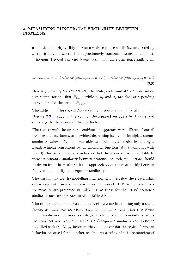
3. MEASURING FUNCTIONAL SIMILARITY BETWEENPROTEINS
semantic similarity visibly increases with sequence similarity, separated by
a transition zone where it is approximately constant. To account for this
behaviour, I added a second NCDF to the modelling function, resulting in:
simfunction = a+b×NCDF (simsequence, µ1, σ1)+c×NCDF (simsequence, µ2, σ2)
(3.9)
Here b, µ1 and σ1 are respectively the scale, mean and standard deviation
parameters for the �rst NCDF , while c, µ2 and σ2 are the corresponding
parameters for the second NCDF .
The addition of the second NCDF visibly improves the quality of the model
(Figure 3.3), reducing the sum of the squared residuals by 14-27% and
centering the dispersion of the residuals.
The results with the average combination approach were di�erent from all
other results, as there was an evident decreasing behaviour for high sequence
similarity values. While I was able to model these results by adding a
negative linear component to the modelling function (d× simsequence, with
d < 0), this behavior clearly indicates that this approach is not suitable to
measure semantic similarity between proteins. As such, no illations should
be drawn from the results with this approach about the relationship between
functional similarity and sequence similarity.
The parameters for the modelling function that describes the relationship
of each semantic similarity measure as function of LRBS sequence similar-
ity measure are presented in Table 3.1, as those for the RRBS sequence
similarity measure are presented in Table 3.2.
The results for the non-electronic dataset were modelled using only a single
NCDF , as there was no visible sign of bimodality and using two NCDF
functions did not improve the quality of the �t. It should be noted that while
the non-electronic results with the RRBS sequence similarity could also be
modelled with the NCDF function, they did not exhibit the typical Gaussian
behavior observed for the other results. As a re�ex of this, parameters of
32
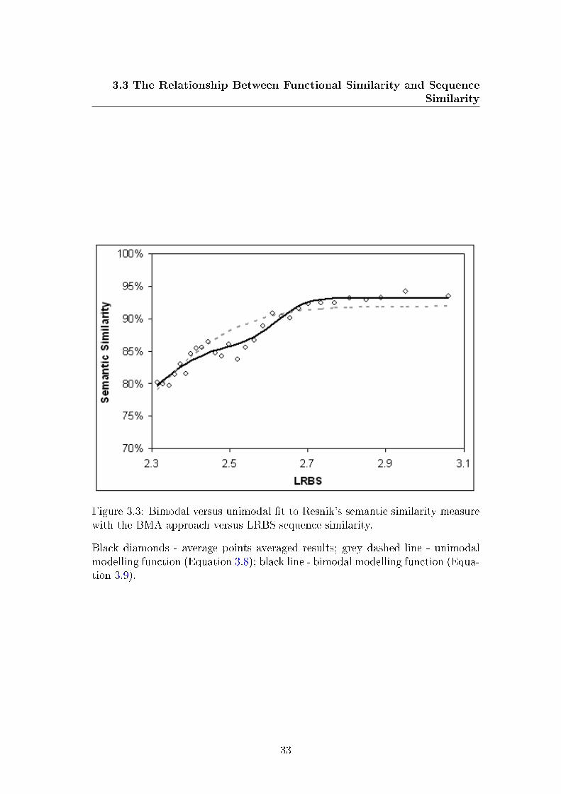
3.3 The Relationship Between Functional Similarity and SequenceSimilarity
Figure 3.3: Bimodal versus unimodal �t to Resnik's semantic similarity measurewith the BMA approach versus LRBS sequence similarity.
Black diamonds - average points averaged results; grey dashed line - unimodalmodelling function (Equation 3.8); black line - bimodal modelling function (Equa-tion 3.9).
33
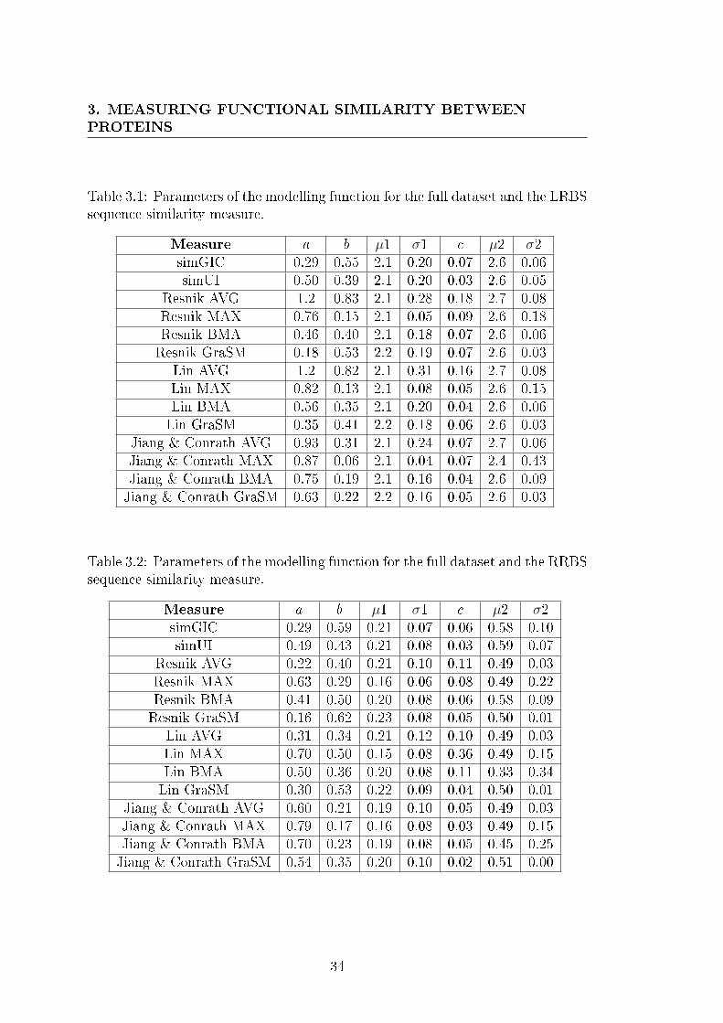
3. MEASURING FUNCTIONAL SIMILARITY BETWEENPROTEINS
Table 3.1: Parameters of the modelling function for the full dataset and the LRBSsequence similarity measure.
Measure a b µ1 σ1 c µ2 σ2simGIC 0.29 0.55 2.1 0.20 0.07 2.6 0.06simUI 0.50 0.39 2.1 0.20 0.03 2.6 0.05
Resnik AVG 1.2 0.83 2.1 0.28 0.18 2.7 0.08Resnik MAX 0.76 0.15 2.1 0.05 0.09 2.6 0.18Resnik BMA 0.46 0.40 2.1 0.18 0.07 2.6 0.06Resnik GraSM 0.18 0.53 2.2 0.19 0.07 2.6 0.03
Lin AVG 1.2 0.82 2.1 0.31 0.16 2.7 0.08Lin MAX 0.82 0.13 2.1 0.08 0.05 2.6 0.15Lin BMA 0.56 0.35 2.1 0.20 0.04 2.6 0.06Lin GraSM 0.35 0.41 2.2 0.18 0.06 2.6 0.03
Jiang & Conrath AVG 0.93 0.31 2.1 0.24 0.07 2.7 0.06Jiang & Conrath MAX 0.87 0.06 2.1 0.04 0.07 2.4 0.43Jiang & Conrath BMA 0.75 0.19 2.1 0.16 0.04 2.6 0.09Jiang & Conrath GraSM 0.63 0.22 2.2 0.16 0.05 2.6 0.03
Table 3.2: Parameters of the modelling function for the full dataset and the RRBSsequence similarity measure.
Measure a b µ1 σ1 c µ2 σ2simGIC 0.29 0.59 0.21 0.07 0.06 0.58 0.10simUI 0.49 0.43 0.21 0.08 0.03 0.59 0.07
Resnik AVG 0.22 0.40 0.21 0.10 0.11 0.49 0.03Resnik MAX 0.63 0.29 0.16 0.06 0.08 0.49 0.22Resnik BMA 0.41 0.50 0.20 0.08 0.06 0.58 0.09Resnik GraSM 0.16 0.62 0.23 0.08 0.05 0.50 0.01
Lin AVG 0.31 0.34 0.21 0.12 0.10 0.49 0.03Lin MAX 0.70 0.50 0.15 0.08 0.36 0.49 0.15Lin BMA 0.50 0.36 0.20 0.08 0.11 0.33 0.34Lin GraSM 0.30 0.53 0.22 0.09 0.04 0.50 0.01
Jiang & Conrath AVG 0.60 0.21 0.19 0.10 0.05 0.49 0.03Jiang & Conrath MAX 0.79 0.17 0.16 0.08 0.03 0.49 0.15Jiang & Conrath BMA 0.70 0.23 0.19 0.08 0.05 0.45 0.25Jiang & Conrath GraSM 0.54 0.35 0.20 0.10 0.02 0.51 0.00
34
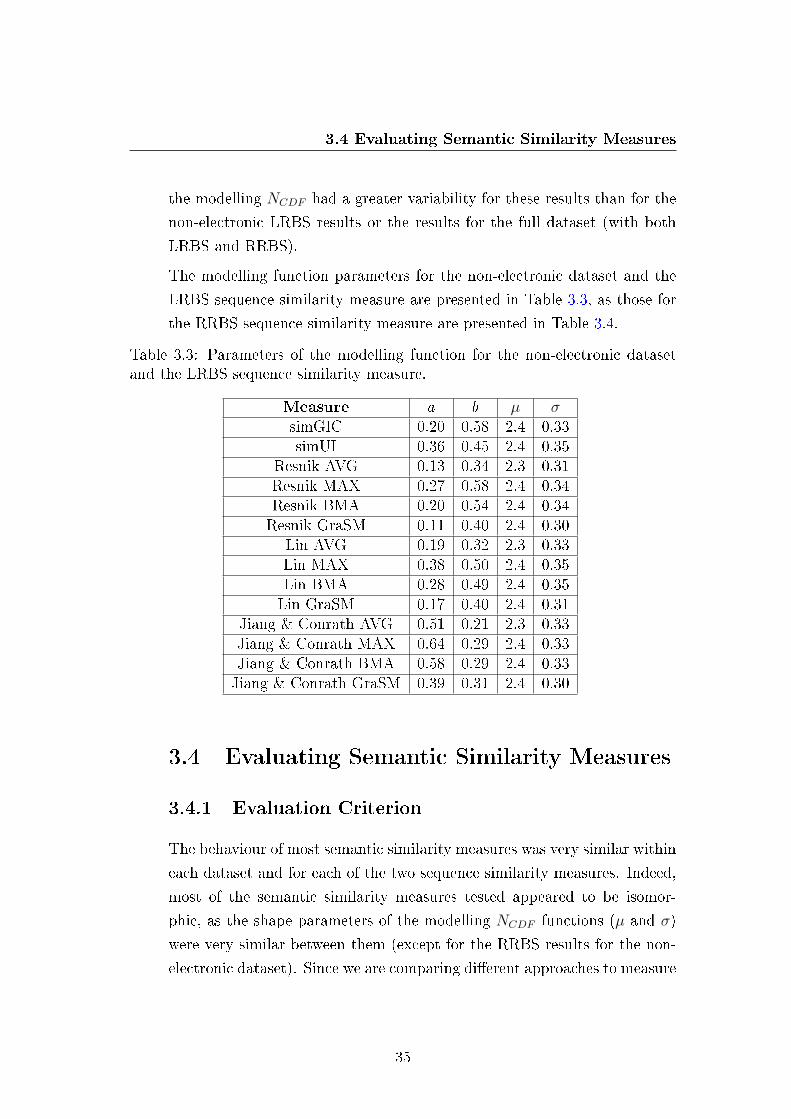
3.4 Evaluating Semantic Similarity Measures
the modelling NCDF had a greater variability for these results than for the
non-electronic LRBS results or the results for the full dataset (with both
LRBS and RRBS).
The modelling function parameters for the non-electronic dataset and the
LRBS sequence similarity measure are presented in Table 3.3, as those for
the RRBS sequence similarity measure are presented in Table 3.4.
Table 3.3: Parameters of the modelling function for the non-electronic datasetand the LRBS sequence similarity measure.
Measure a b µ σsimGIC 0.20 0.58 2.4 0.33simUI 0.36 0.45 2.4 0.35
Resnik AVG 0.13 0.34 2.3 0.31Resnik MAX 0.27 0.58 2.4 0.34Resnik BMA 0.20 0.54 2.4 0.34Resnik GraSM 0.11 0.40 2.4 0.30
Lin AVG 0.19 0.32 2.3 0.33Lin MAX 0.38 0.50 2.4 0.35Lin BMA 0.28 0.49 2.4 0.35Lin GraSM 0.17 0.40 2.4 0.31
Jiang & Conrath AVG 0.51 0.21 2.3 0.33Jiang & Conrath MAX 0.64 0.29 2.4 0.33Jiang & Conrath BMA 0.58 0.29 2.4 0.33Jiang & Conrath GraSM 0.39 0.31 2.4 0.30
3.4 Evaluating Semantic Similarity Measures
3.4.1 Evaluation Criterion
The behaviour of most semantic similarity measures was very similar within
each dataset and for each of the two sequence similarity measures. Indeed,
most of the semantic similarity measures tested appeared to be isomor-
phic, as the shape parameters of the modelling NCDF functions (µ and σ)
were very similar between them (except for the RRBS results for the non-
electronic dataset). Since we are comparing di�erent approaches to measure
35

3. MEASURING FUNCTIONAL SIMILARITY BETWEENPROTEINS
Table 3.4: Parameters of the modelling function for the non-electronic datasetand the RRBS sequence similarity measure.
Measure a b µ σsimGIC -0.01 0.86 0.25 0.32simUI 0.25 0.61 0.29 0.30
Resnik AVG -5.3 5.9 -1.0 0.77Resnik MAX -0.26 1.2 0.08 0.41Resnik BMA -0.80 1.7 -0.11 0.58Resnik GraSM -1.7 2.6 -0.53 1.16
Lin AVG -7.6 8.2 -1.2 0.78Lin MAX 0.11 0.79 0.18 0.34Lin BMA -0.36 1.2 0.01 0.51Lin GraSM -0.30 1.1 0.14 0.60
Jiang & Conrath AVG 0.48 0.27 0.25 0.20Jiang & Conrath MAX 0.63 0.30 0.32 0.17Jiang & Conrath BMA 0.55 0.34 0.32 0.21Jiang & Conrath GraSM 0.34 0.44 0.39 0.27
the same thing (semantic similarity) based on the same data, this similarity
in behavior indicates that most measures are sensitive to the same variations
in the data. This suggests that the pattern captured by most semantic sim-
ilarity measures re�ects the relationship between functional similarity (as
captured by the annotations) and sequence similarity.
If most semantic similarity measures capture functional similarity between
proteins, then evaluating them requires assessing how well they capture
it, or in other words, how sensitive are they to the variations in the an-
notations. Fortunately, assessing this is simply a matter of estimating the
resolution of each measure, which can be done by measuring the range of the
average semantic similarity values as function of sequence similarity. The
resolution of a semantic similarity measure is related to its distribution,
as it measures the average di�erence between proteins with very similar
functions and proteins with very unsimilar functions. Semantic similarity
measures with a higher resolution are more sensitive to small annotation
di�erences, and therefore provide a more accurate measure of functional
similarity. Note, however, that it is only the average behaviour of the se-
36
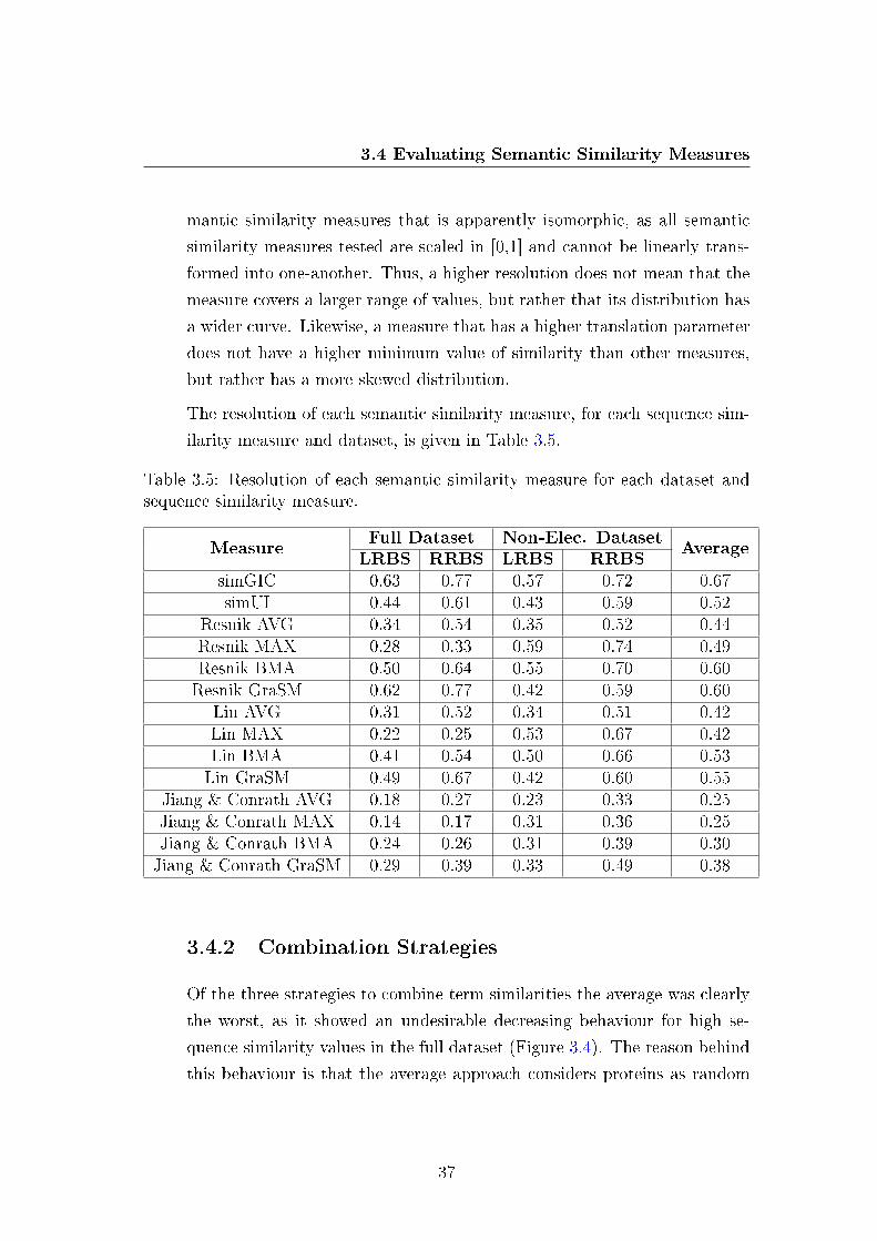
3.4 Evaluating Semantic Similarity Measures
mantic similarity measures that is apparently isomorphic, as all semantic
similarity measures tested are scaled in [0,1] and cannot be linearly trans-
formed into one-another. Thus, a higher resolution does not mean that the
measure covers a larger range of values, but rather that its distribution has
a wider curve. Likewise, a measure that has a higher translation parameter
does not have a higher minimum value of similarity than other measures,
but rather has a more skewed distribution.
The resolution of each semantic similarity measure, for each sequence sim-
ilarity measure and dataset, is given in Table 3.5.
Table 3.5: Resolution of each semantic similarity measure for each dataset andsequence similarity measure.
MeasureFull Dataset Non-Elec. Dataset
AverageLRBS RRBS LRBS RRBS
simGIC 0.63 0.77 0.57 0.72 0.67simUI 0.44 0.61 0.43 0.59 0.52
Resnik AVG 0.34 0.54 0.35 0.52 0.44Resnik MAX 0.28 0.33 0.59 0.74 0.49Resnik BMA 0.50 0.64 0.55 0.70 0.60Resnik GraSM 0.62 0.77 0.42 0.59 0.60
Lin AVG 0.31 0.52 0.34 0.51 0.42Lin MAX 0.22 0.25 0.53 0.67 0.42Lin BMA 0.41 0.54 0.50 0.66 0.53Lin GraSM 0.49 0.67 0.42 0.60 0.55
Jiang & Conrath AVG 0.18 0.27 0.23 0.33 0.25Jiang & Conrath MAX 0.14 0.17 0.31 0.36 0.25Jiang & Conrath BMA 0.24 0.26 0.31 0.39 0.30Jiang & Conrath GraSM 0.29 0.39 0.33 0.49 0.38
3.4.2 Combination Strategies
Of the three strategies to combine term similarities the average was clearly
the worst, as it showed an undesirable decreasing behaviour for high se-
quence similarity values in the full dataset (Figure 3.4). The reason behind
this behaviour is that the average approach considers proteins as random
37
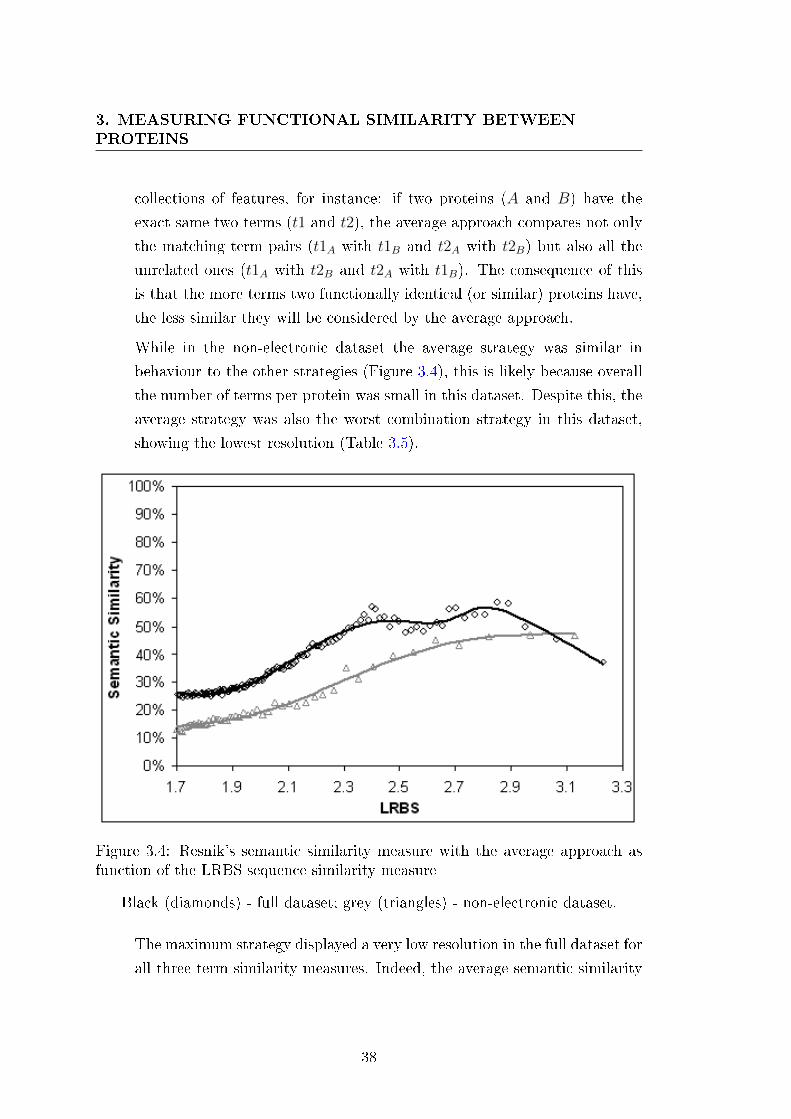
3. MEASURING FUNCTIONAL SIMILARITY BETWEENPROTEINS
collections of features, for instance: if two proteins (A and B) have the
exact same two terms (t1 and t2), the average approach compares not only
the matching term pairs (t1A with t1B and t2A with t2B) but also all the
unrelated ones (t1A with t2B and t2A with t1B). The consequence of this
is that the more terms two functionally identical (or similar) proteins have,
the less similar they will be considered by the average approach.
While in the non-electronic dataset the average strategy was similar in
behaviour to the other strategies (Figure 3.4), this is likely because overall
the number of terms per protein was small in this dataset. Despite this, the
average strategy was also the worst combination strategy in this dataset,
showing the lowest resolution (Table 3.5).
Figure 3.4: Resnik's semantic similarity measure with the average approach asfunction of the LRBS sequence similarity measure
Black (diamonds) - full dataset; grey (triangles) - non-electronic dataset.
The maximum strategy displayed a very low resolution in the full dataset for
all three term similarity measures. Indeed, the average semantic similarity
38
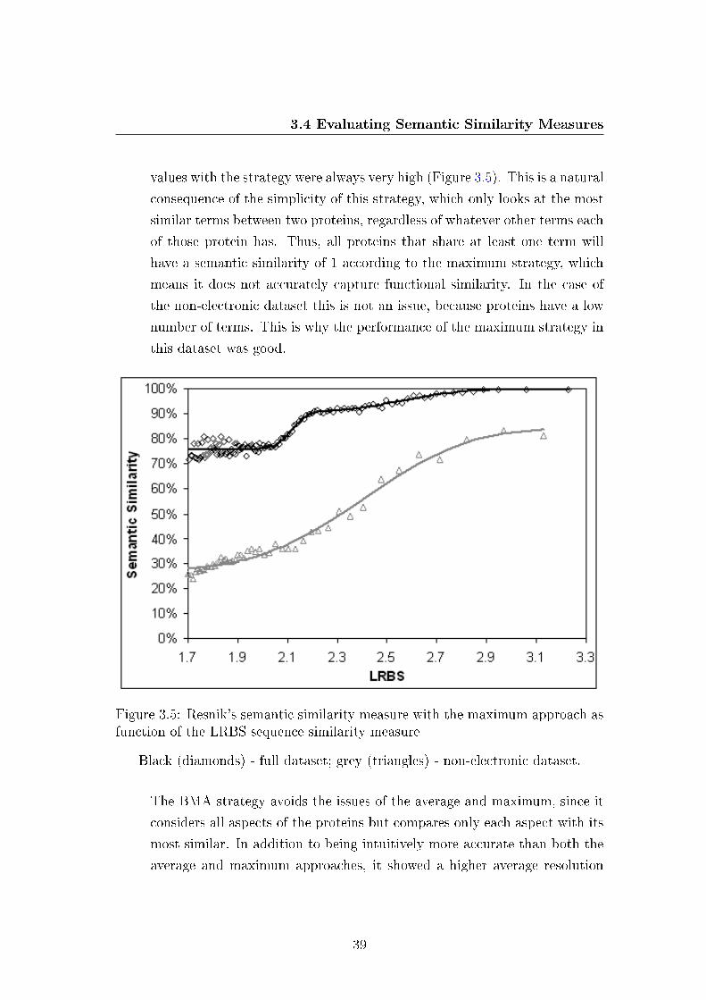
3.4 Evaluating Semantic Similarity Measures
values with the strategy were always very high (Figure 3.5). This is a natural
consequence of the simplicity of this strategy, which only looks at the most
similar terms between two proteins, regardless of whatever other terms each
of those protein has. Thus, all proteins that share at least one term will
have a semantic similarity of 1 according to the maximum strategy, which
means it does not accurately capture functional similarity. In the case of
the non-electronic dataset this is not an issue, because proteins have a low
number of terms. This is why the performance of the maximum strategy in
this dataset was good.
Figure 3.5: Resnik's semantic similarity measure with the maximum approach asfunction of the LRBS sequence similarity measure
Black (diamonds) - full dataset; grey (triangles) - non-electronic dataset.
The BMA strategy avoids the issues of the average and maximum, since it
considers all aspects of the proteins but compares only each aspect with its
most similar. In addition to being intuitively more accurate than both the
average and maximum approaches, it showed a higher average resolution
39
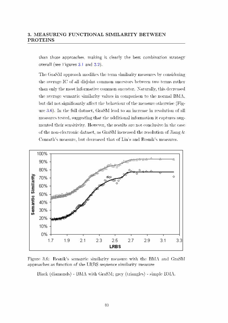
3. MEASURING FUNCTIONAL SIMILARITY BETWEENPROTEINS
than those approaches, making it clearly the best combination strategy
overall (see Figures 3.1 and 3.2).
The GraSM approach modi�es the term similarity measures by considering
the average IC of all disjoint common ancestors between two terms rather
than only the most informative common ancestor. Naturally, this decreased
the average semantic similarity values in comparison to the normal BMA,
but did not signi�cantly a�ect the behaviour of the measure otherwise (Fig-
ure 3.6). In the full dataset, GraSM lead to an increase in resolution of all
measures tested, suggesting that the additional information it captures aug-
mented their sensitivity. However, the results are not conclusive in the case
of the non-electronic dataset, as GraSM increased the resolution of Jiang &
Conrath's measure, but decreased that of Lin's and Resnik's measures.
Figure 3.6: Resnik's semantic similarity measure with the BMA and GraSMapproaches as function of the LRBS sequence similarity measure
Black (diamonds) - BMA with GraSM; grey (triangles) - simple BMA.
40
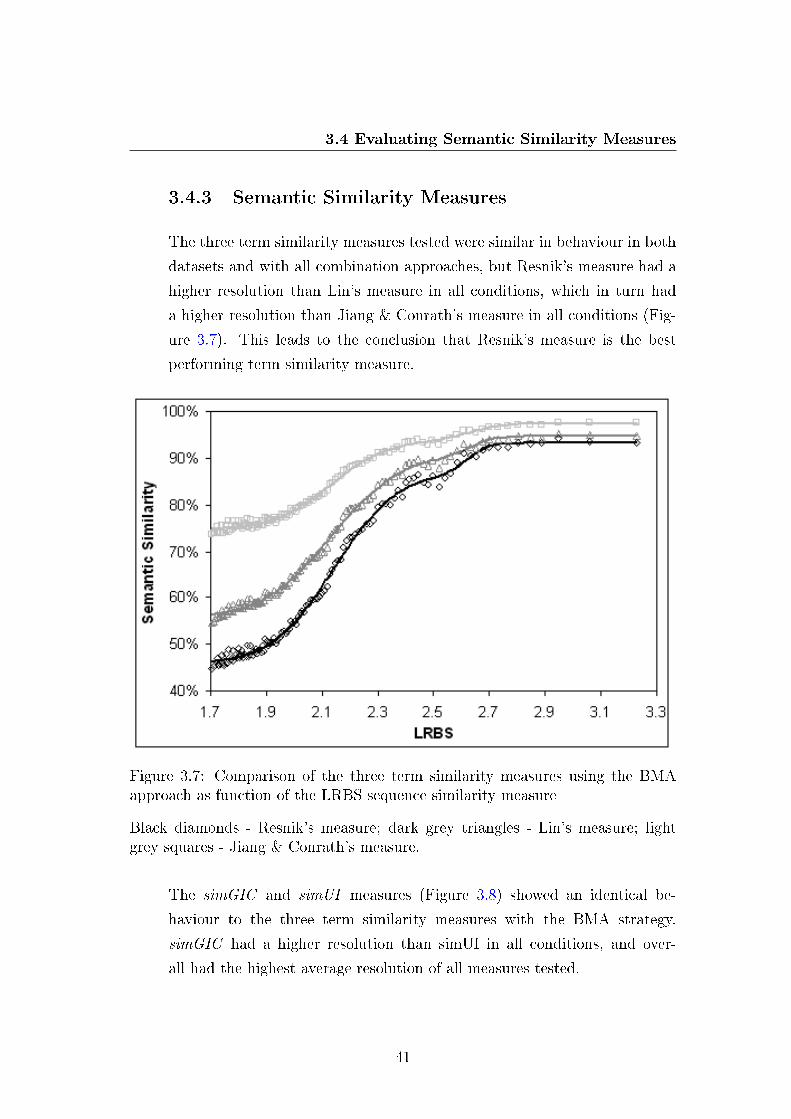
3.4 Evaluating Semantic Similarity Measures
3.4.3 Semantic Similarity Measures
The three term similarity measures tested were similar in behaviour in both
datasets and with all combination approaches, but Resnik's measure had a
higher resolution than Lin's measure in all conditions, which in turn had
a higher resolution than Jiang & Conrath's measure in all conditions (Fig-
ure 3.7). This leads to the conclusion that Resnik's measure is the best
performing term similarity measure.
Figure 3.7: Comparison of the three term similarity measures using the BMAapproach as function of the LRBS sequence similarity measure
Black diamonds - Resnik's measure; dark grey triangles - Lin's measure; lightgrey squares - Jiang & Conrath's measure.
The simGIC and simUI measures (Figure 3.8) showed an identical be-
haviour to the three term similarity measures with the BMA strategy.
simGIC had a higher resolution than simUI in all conditions, and over-
all had the highest average resolution of all measures tested.
41
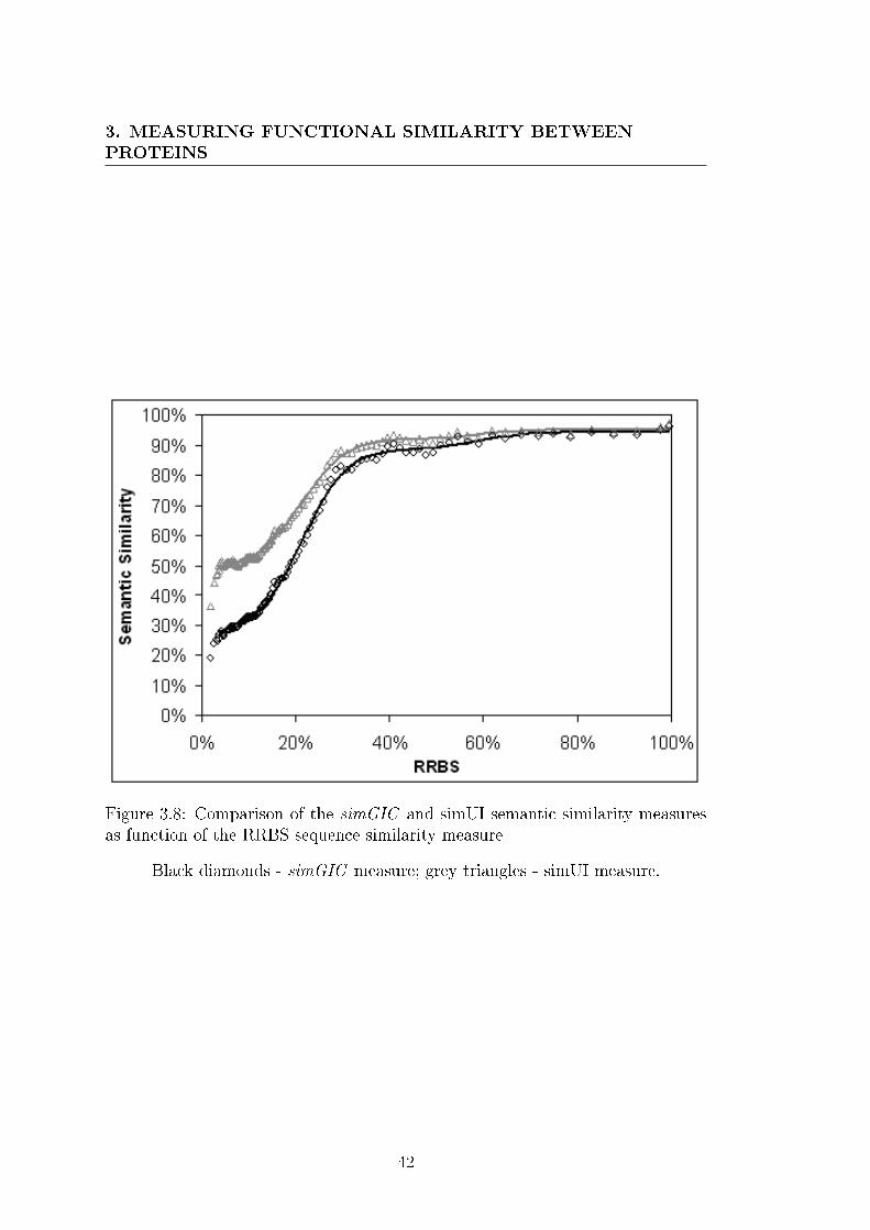
3. MEASURING FUNCTIONAL SIMILARITY BETWEENPROTEINS
Figure 3.8: Comparison of the simGIC and simUI semantic similarity measuresas function of the RRBS sequence similarity measure
Black diamonds - simGIC measure; grey triangles - simUI measure.
42
3.5 Discussion
3.5 Discussion
3.5.1 Electronic versus Manually Curated Annotations
There were two notable di�erences between the results of the full and the
non-electronic dataset: semantic similarity values were lower in the lat-
ter, and it had no visible bimodal behavior. The �rst di�erence can be
explained by the smaller number of annotations per protein in the non-
electronic dataset (2 instead of 3) which makes it less likely that proteins
have annotations in common. The absence of the bimodal behavior can be
due to the smaller size of the non-electronic dataset, as less data provides
less detail about the relationship between function and sequence. However,
it is also possible that the bimodal behavior observed on the full dataset
is an artifact caused by data circularity, as most electronic annotations are
based on sequence similarity. Since functional inferences are predominantly
made at high levels of sequence similarity, if there was a visible in�uence
of data circularity in our results, it would be expected in the form of an
abnormal increase in semantic similarity for high sequence similarity val-
ues. Thus, the hypothesis of data circularity is consistent with the observed
bimodal behavior observed in the full dataset and with its absence in the
non-electronic dataset. Despite this, there is no avoiding the fact that the
full dataset provides a clearer picture of the relationship between function
and sequence than the non-electronic dataset, as non-electronic annotations
cover only a small fraction of proteins and GO terms.
3.5.2 Sequence Similarity Measures
The shape di�erences between the LRBS and RRBS results are mostly due
to the fact that the former measure is logarithmic whereas the latter is
a relative measure. It should be noted that the LRBS is not a suitable
measure of sequence similarity, as it depends directly on the length of the
proteins. In addition to being more intuitive to interpret, RRBS is less
biased and therefore a more suitable measure of sequence similarity. Thus, it
43
3. MEASURING FUNCTIONAL SIMILARITY BETWEENPROTEINS
is unsurprising that the semantic similarity values have a higher correlation
with RRBS than LRBS, which is also translated to a higher coverage of the
semantic similarity scale.
3.5.3 The Relationship Between Sequence and Func-
tion
Ignoring the bimodal behavior, the interpretation of the semantic similar-
ity versus RRBS curve is relatively straightforward. Above 30% sequence
similarity, most proteins have highly similar functions, and the average func-
tional similarity increases only slightly with sequence similarity. This means
that alignment-based protein function predictions above this sequence sim-
ilarity range should be reasonably reliable. However, not even 100% se-
quence similarity is su�cient to ensure 100% semantic similarity, which
is likely caused in part by incomplete and inconsistent annotations, but
also re�ects the existence of cases of divergent evolution. Below 30% se-
quence similarity, function similarity values drop rapidly, which means that
alignment-based protein function predictions will generally be unreliable.
Sequence similarity values between 25 and 30% should be su�cient to in-
fer general functional aspects, but below 25% function even this should be
avoided. In any case, the modelling NCDF function can be used to produce a
reliability score for alignment-based protein function predictions depending
on the quality of the sequence alignments.
3.5.4 Term Similarity Combination Strategies
Regarding the strategies to combine term similarities, it is clear that neither
the average strategy nor the maximum strategy accurately capture func-
tional similarity. The average strategy is negatively biased by the number
of annotations of the proteins being compared, and is innacurate because
it will not return a value of 100% when comparing proteins with multi-
ple identical annotations. The maximum strategy is positively biased by
44
3.5 Discussion
the number of annotations of the proteins being compared (since the more
annotations they have, the more likely they are to have at least one sim-
ilar term), and is inaccurate because it will return a value of 100% when
comparing proteins that share a minor functional aspect (such as iron ion
binding) but have otherwise di�erent functions. The fact that these strate-
gies produced good results in the non-electronic dataset was due to the low
number of annotations per protein and should not justify their use. The
BMA strategy is clearly the most suitable strategy for combining term sim-
ilarities, as it is not biased by the number of annotations of the proteins
compared and had a higher average resolution than both the average and
maximum strategies.
3.5.5 Semantic Similarity Measures
Resnik's measure was the best of the term similarity measures tested, as
it consistently showed a higher resolution than both Lin's and Jiang &
Conrath's measures. Resnik's measure using the BMA combination strat-
egy was the second best approach to calculate functional similarity, as its
average resolution was only below that of the simGIC measure.
The e�ect of the GraSM approach appeared to be positive, as it increased
the resolution of the term-based measures in the full dataset. However,
the results were not fully conclusive, as this approach had the opposite
e�ect for two of the term-based measures in the non-electronic dataset.
It is possible that increase in sensitivity obtained by considering multiple
disjoint ancestors is only relevant when comparing proteins with multiple
and more detailed annotations.
Overall, simGIC had the highest average resolution, and either the high-
est or second highest resolution for each dataset and sequence similarity
measure. Thus, it was clearly the best of the semantic similarity measures
tested. Additionally, simGIC is computationally much simpler than the
term-based measures, as it can be computed in a single step without the
45

3. MEASURING FUNCTIONAL SIMILARITY BETWEENPROTEINS
need to �nd matching terms. Thus, it is computationally advantageous, in
addition to being a more sensitive semantic similarity measure.
It was interesting to note that the simUI measure had an identical be-
haviour to simGIC. This indicates that employing the concept of IC is not
essential to measure semantic similarity accurately. However, the fact that
simUI had a lower resolution than simGIC, considering that they are oth-
erwise identical, leads to the conclusion that using the IC improves the
sensitivity of a semantic similarity measure.
46
Chapter 4
Improving Annotation
Consistency
4.1 Background
The foundation of the Gene Ontology (GO) was a huge step in the path
towards objective descriptions of protein functions (The Gene Ontology
Consortium, 2000). But while GO has become the de facto standard for
describing protein functions (Friedberg, 2006), it is far from a �nished prod-
uct. Indeed, GO has to be constantly updated, not only because our knowl-
edge of biological phenomena is ever increasing, but also because the need
for computability is ever more pressing (Alterovitz et al., 2010; Leonelli
et al., 2011). An example of this is the ongoing update undertaken by the
GO Consortium to normalize and extend the ontology with computable log-
ical de�nitions, including references to external ontologies (Mungall et al.,
2011). In addition to facilitating computer reasoning, this update will allow
the development of GO to be partially automated.
Having an ontology to represent protein functions only takes us halfway
through the path towards objective descriptions of protein functions, as it
is also necessary that that ontology be used objectively and consistently for
annotating proteins. If proteins that have the exact same function are not
47

4. IMPROVING ANNOTATION CONSISTENCY
described consistently with the same set of annotations, this undermines
the very purpose of having an ontology for annotation, and may lead to a
scenario where we are not able to reliably identify the function of a protein
from its annotations.
Even amongst GO curators annotation agreement is not perfect (Camon
et al., 2005). However, the inconsistency of manually curated annotations
is a very minor issue considering that over 98% of the annotations of UniPro-
tKB proteins are electronically inferred (as of the GOA release of October
2010). Being mostly based on sequence alignments, electronic annotations
are generally considered unreliable (Jones et al., 2007), but they are also
probably very inconsistent, since they are not manually veri�ed, and pro-
teins can receive electronic annotations from various independent and un-
coordinated data sources.
Unfortunately, this issue has been largely unaddressed, as most researchers
analyzing GO annotations have eschewed electronic annotations altogether
(Bada et al., 2004; Bodenreider et al., 2005; Kumar et al., 2004). Given that
manual curation of all functional annotations is beyond present or foresee-
able resources (Barrell et al., 2009), improving the quality and consistency
of electronic annotations should be a research priority. While there are gen-
eral issues about their reliability, electronic annotations also include some
high-quality annotations, such as those inferred from manually curated EC
family assignments or those inferred from manually analyzed InterPro sig-
natures (Barrell et al., 2009; Camon et al., 2005). Improving the consistency
of electronic annotations will facilitate the functional comparison of proteins
based on their annotations, which can contribute to assess the quality and
reliability of those annotations, and help identify annotation errors.
With the goal of improving annotation consistency, I developed a data min-
ing algorithm, based on association rule learning (ARL), to �nd implicit re-
lationships between molecular function terms. While ARL approaches have
been previously employed to �nd relationships between GO terms, they fo-
cused on relationships between terms of di�erent GO categories, and did
48
4.2 Methods
not consider electronic annotations (Bada et al., 2004; Bodenreider et al.,
2005; Kumar et al., 2004).
In this chapter, I study how protein functions are represented by molecu-
lar function annotations, assess the consistency of those annotations, and
evaluate the algorithm for �nding relationships between molecular function
terms.
4.2 Methods
4.2.1 Dataset
This work was based on the release 4.2 of the FunSimMat database, which
compiles protein and annotation data from the UniProtKB, annotation data
from GOA, and ontology data from GO, as of the respective releases of Oc-
tober 2010 (Schlicker & Albrecht, 2010). The dataset comprises 7.3 million
annotated UniProtKB proteins, 21 million molecular function annotations
(of which 99.4% are inferred electronically) and 8889 non-obsolete molecular
function terms.
4.2.2 Redundant Annotations
An annotation is redundant if it is implied by another more speci�c anno-
tation of the same protein. For instance, if a protein is annotated to both
heme binding and its parent term iron ion binding, the latter annotation
is redundant as it is already implied by the former annotation through the
structure of the ontology.
4.2.3 Incomplete Annotations
To estimate the number of incomplete annotations, I employed the descendent-
based information content (dIC), which is analogous to the traditional
annotation-based information content (aIC), but is based on the structure
49

4. IMPROVING ANNOTATION CONSISTENCY
of the ontology rather than the annotation of the terms. The dIC of a term
is given by the negative logarithm of the fraction of ontology terms that
are descendents of that term (including itself). Whereas the aIC measures
informativeness, the dIC measures speci�city (i.e. the level of detail within
the ontology), which is more directly related to completeness. For instance,
all leaf terms correspond to complete functional (within the current limits
of the ontology) aspects and accordingly all have a dIC of 100%, but their
aIC ranges from 12% to 100%.
The assumption in employing the dIC is that a protein which is anno-
tated non-redundantly with any non-speci�c term is incompletely anno-
tated. While this is generally true, it covers only part of the incomplete
annotations, since proteins may have completely unknown functional as-
pects which are absent from the annotations.
I selected a dIC threshold of 73% in order to capture cases of non-leaf terms
that correspond to reasonably complete functional aspects. Examples in-
clude the term iron ion binding, which represents a complete functional as-
pect, despite having the child heme binding, and the term sequence-speci�c
DNA binding transcription factor activity which has several descendents
but is used directly for annotation more often that all those descendents
combined. This threshold of 73% is relaxed, as it leaves out only the 5%
most generic molecular function terms. Nevertheless, it is preferable to
make a liberal estimation of the number of completely annotated proteins
than to exclude cases such as the previous examples.
4.2.4 MFclasses
Describing a protein function typically requires more than one molecular
function term. Thus, we can consider that each molecular function term cor-
responds to a functional aspect, and each unique combination of molecular
function terms, or MFclass, corresponds to a protein function. For instance,
consider the MFclass comprising the terms two-component response regu-
lator activity, sequence-speci�c DNA binding transcription factor activity
50

4.2 Methods
and sequence-speci�c DNA binding (and implicitly, their ancestors) which
is typically used to describe two-component response regulator proteins that
act upon the transcription process. Each term individually describes only
an aspect of this function, and it takes the combination of the three terms
(the MFclass) to fully describe the function.
The concept of MFclass is extremely useful to study the annotation space,
since proteins that belong to the same MFclass are redundant from a func-
tional perspective. In particular, this concept is essential to study inconsis-
tent annotations.
4.2.5 Inconsistent Annotations
Two proteins are inconsistently annotated if they have the same function
but are not annotated to the same set of molecular function terms, and thus
do not belong to the same MFclass. This might be due to di�erences in an-
notation criteria, to minor annotation errors, or to the lack of coordination
between annotation sources. In any case, the result is that there are two
or more (typically similar) MFclasses that actually correspond to the same
protein function. For example, most transcription factors involved in two-
component response systems are annotated to the terms: two-component
response regulator activity, sequence-speci�c DNA binding transcription fac-
tor activity and sequence-speci�c DNA binding. However, others are only
annotated to the �rst two terms, which is an evident case of inconsistent
annotation, as it is clear that both sets of annotations describe the same
function.
In order to assess how common inconsistent annotations are, I analyzed
manually the 100 most frequently annotated MFclasses that include more
than one term. For each of those MFclasses, I identi�ed the primary (or
function-de�ning) terms and searched for additional MFclasses that include
those terms, but have minor di�erences. In order to assess whether the
MFclasses found correspond to the same function, I searched for information
51
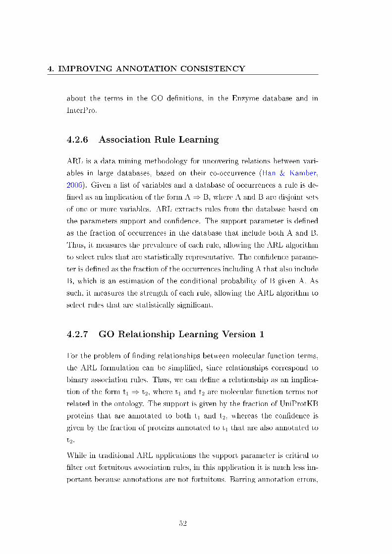
4. IMPROVING ANNOTATION CONSISTENCY
about the terms in the GO de�nitions, in the Enzyme database and in
InterPro.
4.2.6 Association Rule Learning
ARL is a data mining methodology for uncovering relations between vari-
ables in large databases, based on their co-occurrence (Han & Kamber,
2006). Given a list of variables and a database of occurrences a rule is de-
�ned as an implication of the form A⇒ B, where A and B are disjoint sets
of one or more variables. ARL extracts rules from the database based on
the parameters support and con�dence. The support parameter is de�ned
as the fraction of occurrences in the database that include both A and B.
Thus, it measures the prevalence of each rule, allowing the ARL algorithm
to select rules that are statistically representative. The con�dence parame-
ter is de�ned as the fraction of the occurrences including A that also include
B, which is an estimation of the conditional probability of B given A. As
such, it measures the strength of each rule, allowing the ARL algorithm to
select rules that are statistically signi�cant.
4.2.7 GO Relationship Learning Version 1
For the problem of �nding relationships between molecular function terms,
the ARL formulation can be simpli�ed, since relationships correspond to
binary association rules. Thus, we can de�ne a relationship as an implica-
tion of the form t1 ⇒ t2, where t1 and t2 are molecular function terms not
related in the ontology. The support is given by the fraction of UniProtKB
proteins that are annotated to both t1 and t2, whereas the con�dence is
given by the fraction of proteins annotated to t1 that are also annotated to
t2.
While in traditional ARL applications the support parameter is critical to
�lter out fortuitous association rules, in this application it is much less im-
portant because annotations are not fortuitous. Barring annotation errors,
52
4.2 Methods
any co-occurrence of molecular function terms should be biologically mean-
ingful. Thus, I opted for a support threshold of 10 proteins (or 0.00014%)
which should be su�cient to ensure the relationships are reliable while ac-
counting for the possibility of annotation errors. On the other hand, the
con�dence parameter is more critical than in traditional ARL applications,
since the goal is to �nd relationships that can potentially be integrated
into GO. However, the fact that there are inconsistent annotations means
that we cannot expect even strong relationships to be true for all proteins.
Thus, taking into consideration the percentage of inconsistently annotated
proteins I found when analysing molecular function annotations, I opted for
a con�dence threshold of 80%.
The main issue of this application of the ARL methodology is that it is
unprepared to deal with hierarchically structured data (Srikant & Agrawal,
1995). Given the hierarchical relationships of the GO structure, ARL will
tend to capture multiple redundant associations and associations between
generic terms. For instance, if the association rule t1 ⇒ t2 has a support
S and con�dence C, then every association rule of the form t1 ⇒ ti (where
ti is an ancestor of t2) will have a support S' ≥ S and a con�dence C' ≥C. The reason for this is that the annotations of t2 are inherited by all of
its ancestors, and thus a co-occurrence of t1 and t2 is also a co-occurrence
of t1 and every ancestor of t2. Thus, if the more speci�c association rule
is accepted by ARL, all ancestral rules will also be accepted. Note that
association rules of the form tj ⇒ t2 (where tj is an ancestor of t1) will also
have a support S' ≥ S but may have a lower con�dence. Thus, ancestral
rules of this form may or may not be accepted.
To address this issue, I excluded relationships that include generic terms
(i.e. terms with more than 10 descendents) and all relationships that were
ancestral to any other predicted relationship. Note that it is possible that in
some cases the true relationship is not the most speci�c one, but such cases
are trivial to identify for a GO curator. Furthermore, relationships between
high level terms are uninteresting for the purpose of improving annotation
consistency, even if they are true. Finally, in the cases where a relationship
53
4. IMPROVING ANNOTATION CONSISTENCY
was predicted in both directions, I excluded one of the directions. Again,
identifying the correct direction of a relationship is trivial for a GO curator,
and returning a relationship in both directions would be redundant.
Another issue of this application of ARL is that GO is not a strict hier-
archy, since terms can have shared descendents. Two terms that are not
directly related in the ontology but have one or more shared descendents
will evidently have their co-occurrence conditioned by the occurrence of
those shared descendents. Thus, we cannot assume that such terms are
directly related based on their co-occurrence. To account for these cases,
I excluded relationships between terms that have close shared descendents
(i.e. a descendent distance of 4 of less edges).
Additionally, I also excluded relationships between terms that have close
shared ancestors (i.e. an ascendent distance of 4 of less edges), which gen-
erally correspond to cases of bifunctional proteins. In order to improve
annotation consistency, I want to �nd relationships between aspects of pro-
tein functions, where the presence of a given aspect implies the other as-
pects. Relationships between functions that are logically independent (even
in cases where all know proteins are bifunctional) are uninteresting from this
perspective.
In summary, the GO relationship learning algorithm (GRL1) retrieves all
relationships of the form t1 ⇒ t2 such that:
� t1 and t2 both have at most 10 descendents (i.e. are leaf or near-leaf
terms).
� t1 and t2 are co-annotated to at least 10 proteins (support).
� t2 is annotated to at least 80% of the proteins that are annotated to
t1 (con�dence).
� The descendent distance between t1 and t2 is greater than 4 edges (i.e.
the terms have no close shared descendents).
� The ancestral distance between t1 and t2 is greater than 4 edges (i.e.
the terms have no close shared ancestors).
54
4.2 Methods
� The criteria above are not met by any relationship of the form t1D ⇒t2, t1 ⇒ t2D or t1D ⇒ t2D, where t1D is a descendent of t1 and t2D is
a descendent of t2.
� If t2 ⇒ t1 meets the criteria above, only one of the pair of relationships
is returned.
4.2.8 GO Relationship Learning Version 2
One limitation of the con�dence parameter is that it doesn't distinguish
between relationships that have exceptions due to inconsistent annotations
and relationships that have biologically meaningful exceptions. For in-
stance, the association rule oxygen transporter activity ⇒ heme binding has
an above threshold con�dence (83%) due to the popularity of hemoglobins,
but there are oxygen transporters with other cofactors such as hemerythrins
(non-heme iron) or hemocyanins (copper).
While distinguishing between functional variants and inconsistent annota-
tions is virtually impossible to do automatically, we can expect that the
former lead to greater annotation variability than the latter, since each
functional variant will likely have its own inconsistent annotations. Thus,
we can expect that in general cases of functional variants will lead to a
larger fraction of MFclasses that do not support the relationship in ques-
tion than cases where there are only inconsistent annotations. As such, I
added another parameter to the GRL1 algorithm, called agreement, in or-
der to �lter out relationships with biologically meaninful exceptions. The
agreement is analogous to the con�dence, but is based on the number of
MFclasses, rather than the number of proteins. For a given relationships t1⇒ t2, the agreement is de�ned as the fraction of MFclasses containing t1that also contain t2. Relationships that have a high agreement will have few
distinct exceptions, and thus those exceptions are more likely to be cases
of inconsistent annotations (which I want to capture) than to be functional
variants (which I don't).
55
4. IMPROVING ANNOTATION CONSISTENCY
The GRL2 algorithm is otherwise identical to the GRL1 algorithm, but uses
an agreement threshold of 80% in addition to the con�dence threshold of
80% to �lter relationships.
4.2.9 Evaluation of the GRL algorithms
In order to assess the precision (i.e. the fraction of true predictions) of
the relationships predicted by GRL1 and GRL2, I evaluated manually the
top 100 relationships of both algorithms as ranked by support. I looked for
evidences supporting or refuting each association in GO, Enzyme, InterPro,
Brenda (Scheer et al., 2011), and when necessary by doing a bibliography
search. I classi�ed relationships as true when I found evidence supporting
their validity for all known proteins; as reverse if the relationships was true
in the reverse direction; as unknown if evidence was inconclusive; and as
false if at least one counterexample is known.
For the purpose of estimating precision, I considered reverse relationships as
true positives, since the algorithms are intended for assisting curators, which
can readily identify the correct direction of a relationship. I considered
unknown relationships as false positives, to make a conservative estimation
of the precision.
4.3 Exploring the Annotation Space
4.3.1 Redundant Annotations and Incomplete Anno-
tations
Upon analyzing the GO molecular function annotations per protein, it is
readily apparent that many proteins have redundant annotations. Indeed
38% of the GO molecular function annotations are redundant. While re-
dundant annotations are a relatively minor issue, they are also relatively
trivial to address, and doing so would reduce database space considerably
and facilitate computations based on annotations. It must be noted that a
56
4.3 Exploring the Annotation Space
redundant annotation should not be discarded if it is based on a stronger
evidence than the more speci�c annotation. However, there are hardly rea-
sons to keep redundant annotations that are inferred electronically, and
these represent 99% of all redundant annotations.
It is also readily apparent that many proteins have non-redundant annota-
tions to top level molecular function terms such as binding (265,000 pro-
teins) or catalytic activity (219,000 proteins). Overall, 64% of all proteins
have one non-redundant annotation to one of the 5% most generic molecu-
lar function terms. This indicates that their functions are not fully known
or possibly that GO lacks the terms required to describe their functions in
more detail. Regardless of the cause, these are cases where the annotations
are not su�ciently detailed to fully describe the function of the proteins,
or in other words, cases of incomplete annotations. Under this estimation,
the number of completely annotated proteins is only 2.6 million (or 36% of
all annotated proteins).
While incompletely annotated proteins are an unavoidable consequence of
our incomplete knowledge of protein functions, it is worth mentioning that
33% of the molecular function near-leaf and leaf terms are not currently in
use to annotate any protein, which suggests that GO annotation sources are
not keeping up with GO updates. Thus, it is likely that some proteins are
incompletely annotated because their annotations were based on an older
and less detailed version of the ontology.
4.3.2 De�ning Protein Function
Proteins are typically annotated to multiple non-redundant molecular func-
tion terms, which means that a protein function corresponds to a unique
combination of molecular function terms, or MFclass. The 2.6 million com-
pletely annotated proteins correspond to 14,317 distinct (complete) MF-
classes. Some of these MFclasses (22%) comprise only one non-redundant
term, but the large majority (75%) have between 2 and 5 terms (Figure
4.1). Although the number of terms per MFclass ranges up to 17, there are
57
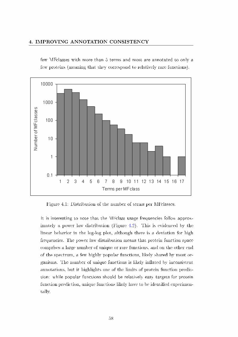
4. IMPROVING ANNOTATION CONSISTENCY
few MFclasses with more than 5 terms and most are annotated to only a
few proteins (meaning that they correspond to relatively rare functions).
Figure 4.1: Distribution of the number of terms per MFclasses.
It is interesting to note that the MFclass usage frequencies follow approx-
imately a power law distribution (Figure 4.2). This is evidenced by the
linear behavior in the log-log plot, although there is a deviation for high
frequencies. The power law distribution means that protein function space
comprises a large number of unique or rare functions, and on the other end
of the spectrum, a few highly popular functions, likely shared by most or-
ganisms. The number of unique functions is likely in�ated by inconsistent
annotations, but it highlights one of the limits of protein function predic-
tion: while popular functions should be relatively easy targets for protein
function prediction, unique functions likely have to be identi�ed experimen-
tally.
58

4.3 Exploring the Annotation Space
Figure 4.2: Distribution of the usage frequency of MFclasses with power lawregression curve.
59
4. IMPROVING ANNOTATION CONSISTENCY
4.3.3 Inconsistent Annotations
Identifying inconsistent annotations is far from straightforward. We can
de�ne inconsistent annotations as cases where two or more (typically simi-
lar) MFclasses are actually describing the same function. However, without
manual analysis, it is virtually impossible to distinguish between cases of
similar MFclasses that correspond to inconsistent annotations from cases
of similar MFclasses that correspond to similar but distinct functions. For
instance, hemoglobins and hemerythrins are two types of iron-containing
oxygen transporting proteins that di�er only in the presence or absence
of an heme group. As such, they are described by very similar MFclasses
that correspond to similar functions. On the other hand, some hemoglobins
are inconsistently annotated, lacking the term oxygen transporter activity.
Based on the similarity of their annotations, the hemerythrins would more
likely be identi�ed as inconsistently annotated than the actual inconsistently
annotated hemoglobins.
The homology-based approach proposed by Dolan et al. (2005) for assess-
ing annotation consistency is unfortunately not applicable on the scale of
the UniProtKB. On the one hand, not all proteins have close homologues,
and �nding homologues for all annotated UniProtKB proteins that do have
them would be a monumental task. On the other hand, even close homo-
logues may have diverged to perform similar but not equal functions, and
so manual analysis would be needed to distinguish cases of inconsistently
annotated homologues from cases of divergent homologues.
In my manual analysis of the top 100 MFclasses, I found that for 88 of
those MFclasses there was at least one other MFclass corresponding to an
inconsistent variant of the same function. Furthermore, 3 of the remain-
ing 12 MFclasses did not correspond to complete functions and thus were
impossible to analyze for inconsistencies. This means that only 9 of the
MFclasses I analyzed correspond univocally to a protein function, and this
is counting only evident cases of inconsistency. For instance, my analy-
sis would not capture major inconsistencies such as that described for the
hemoglobins, where one of the primary terms is missing. Assuming that
60
4.3 Exploring the Annotation Space
the most common MFclass describing each function is the correct represen-
tation, the number of inconsistently annotated proteins corresponds to over
20% of the proteins under analysis (which were almost 1 million).
In the large majority of the inconsistent annotations I found in my anal-
ysis, the inconsistency consisted of the presence or absence of a binding
term that described a molecular interaction implicitly implied by a pri-
mary term. There were many cases where the binding term described an
enzyme-substrate or transporter-target interaction evidently implied by the
catalytic/transporter activity term, and described in the de�nition of that
term. There were also many cases where the binding term described an
enzyme-cofactor interaction, which was less evident because the interaction
was not described in the de�nition of the catalytic activity term (although
it is generally described in the corresponding EC family de�nition). The
reason behind these inconsistent annotations is tied to an apparent disagree-
ment about the use of binding terms. On the one hand, the GO annota-
tion conventions state that implicitly implied interactions such as enzyme-
substrate or transporter-target are redundant and should be avoided (al-
though enzyme-cofactor interactions are acceptable). On the other hand,
most GO annotation sources (particularly InterPro) continue to use bind-
ing terms to represent implicitly implied interactions, because having them
explicitly represented as annotations is useful for making sequence-based
annotation inferences as well as for comparing proteins based on their in-
teractions. Thus, the issue is essentially about the accessibility of this infor-
mation, as it is currently present in GO only in the form of human-readable
de�nitions.
The number of inconsistent annotations caused by this issue is likely in the
millions, as there are 2.8 million proteins annotated with both a catalytic
activity term and binding term and another 2 million proteins annotated to
a catalytic activity term but not to a binding term. For instance, there are
275,000 proteins annotated with both ATPase activity and ATP binding,
which is an evident representation of enzyme-substrate binding. But there
are also 29 thousand proteins annotated with ATPase activity but not ATP
61
4. IMPROVING ANNOTATION CONSISTENCY
binding, in accordance with the GO annotation conventions. Additionally,
this issue also leads to cases of incomplete annotations, since the binding
branch is not extensive and does not cover all possible substrates for all
catalytic activity terms. This leads to the use of generic binding terms,
and often the term binding itself to describe interactions. Currently, there
are over 150,000 proteins with an annotation to a catalytic activity term
and a non-redundant annotation to the term binding. Typical examples are
the MFclasses {L-malate dehydrogenase activity ; binding} and {pyrroline-
5-carboxylate reductase activity ; binding} that have very speci�c catalytic
activity terms for which there are no corresponding substrate binding terms.
Given the di�culty in identifying inconsistent annotations, it becomes clear
that the focus should be on preventing them. In order to do that, these im-
plicit molecular interactions must be represented explicitly in the ontology
in a manner amenable to computation. One solution would be to repre-
sent these interactions as relationships between catalytic activity or trans-
porter activity terms and the corresponding binding terms. This would
make the co-annotations with the binding terms actually redundant and
would preclude inconsistent annotations, since the binding term would al-
ways be present by the true path rule. While it would increase the number
of redundant annotations, these could be easily identi�ed and discarded.
The main problem with this solution is that it would change the scope of
the molecular function ontology by dividing functions into steps or parts,
which is likely why GO curators have decided against adopting it. There is,
however, an ongoing upgrade to GO that will provide an alternative solu-
tion, which is the extension of the ontology with cross-products and logical
de�nitions (Mungall et al., 2011). If the information about molecular in-
teractions such as enzyme-substrate or transporter-target is made available
in the form of computable logical de�nitions of the catalytic activity or
transporter activity terms, then it will be unnecessary to represent that
information in the form of annotations. Nevertheless, this solution will not
make the binding annotations actually redundant, and thus it may be nec-
essary to complement it with a more strict enforcement of GO annotation
conventions.
62
4.4 Finding Relationships Between Molecular Function Terms
4.4 Finding Relationships Between Molecular
Function Terms
4.4.1 GO Relationship Learning Results
The GRL1 algorithm extracted 1,101 relationships from the molecular func-
tion annotation space, out of almost 500,000 potentially related molecular
function term pairs (i.e. pairs of terms not related in the ontology that have
at least one co-annotation). The GRL2 algorithm was more selective than
GRL1, reducing the number of predicted relationships by 50% (to 550) due
to the introduction of the agreement parameter.
Of the top 100 relationships predicted by GRL1, 78 were classi�ed as true, 5
as reverse, 9 as unknown, and 8 as false, leading to an estimated precision of
83%. Regarding GRL2, 92 relationships were classi�ed as true, 2 as reverse,
4 as unknown, and 2 as false, leading to an estimated precision of 94%. It
should be noted that, unlike precision, I cannot estimate the recall of the
two algorithms, since I do not know a priori how many true relationships
exist. However, by comparing the results of the two algorithms, I can
assess that GRL2 had a lower recall than GRL1, since 45 of the GRL1
predictions evaluated as true (or reverse) were not present in the GRL2
predictions. Thus, while the introduction of the agreement parameter lead
to an estimated increase in precision of 11%, it also led to an estimated
decrease in recall of 45%.
The manually evaluated top 100 relationships of the two algorithms are
presented in Appendix A.
4.4.2 Comparison with Association Rule Learning
Applying the basic ARL methodology with only the support and con�dence
thresholds would result in 12,352 predicted relationships, with an estimated
precision of only 5%. 9,604 of the relationships predicted by ARL include
generic terms, and all relationships in the top 100 (ranked by support) are
63

4. IMPROVING ANNOTATION CONSISTENCY
generic relationships such as nucleotide binding ⇒ catalytic activity or nu-
cleoside binding ⇒ nucleotide binding. The usefulness of these relationships
is very limited for the purpose of improving annotation quality, so consid-
ering that relationships need to be manually reviewed by GO curators,
excluding these generic relationships is a critical step.
ARL also captures 163 relationships between terms that have close shared
descendents. These should be excluded since they do not correspond to
direct relationships, but rather are indirect relationships through the shared
descendents. A clear example of this is the relationship tetrapyrrole binding
⇒ iron ion binding, which has a support of 259,620 proteins and a con�dence
of 96%, but is due to the shared descendent heme binding (which accounts
for all but 1 of the co-annotations of this pair of terms).
Additionally, ARL captures 506 relationships between term pairs that have
a close shared ancestor. The reason why I excluded these cases was not be-
cause they aren't direct relationships, but rather because they typically do
not correspond to relationships between functional aspects that are part of a
single function, which were the cases I was interested in �nding. Generally,
relationships between sister or closely related terms either correspond to bi-
functional proteins or to synonymous or partially synonymous terms (which
should be related in the ontology but are not). An example of the former is
the relationship asparagine-tRNA ligase activity ⇒ aspartate-tRNA ligase
activity, which describes two logically distinct yet co-occurring functions,
rather than two aspects of a single function (e.g. asparagine-tRNA ligase ac-
tivity ⇒ ATP binding). Examples of the latter include glycerol-3-phosphate
dehydrogenase [NAD(P)+] activity ⇒ glycerol-3-phosphate dehydrogenase
[NAD+] activity. Cases like this reveal structural issues of the ontology,
but they correspond to the same functional aspect described by two di�er-
ent terms, rather than di�erent functional aspects.
Finally, after excluding the cases above, ARL would still capture 978 re-
dundant relationships. Again, excluding these relationships is essential to
facilitate the task of GO curators.
64
4.4 Finding Relationships Between Molecular Function Terms
4.4.3 Discussion
As I discussed in section 4.3.3, preventing inconsistent annotations can be
achieved by enriching GO and/or strictly enforcing annotation conventions.
In either case, it is necessary to identify knowledge that is currently not
expressed explicitly in GO, but may be expressed in the annotations. The
GRL algorithms can aid GO curators by retrieving this knowledge from the
GO annotations, and thus can be useful to improve annotation consistency.
The GRL1 algorithm was highly selective, with a high estimated precision
(83%) when compared with the basic ARL methodology (5%). While it
is likely that GRL1 missed some true relationships, and thus has a lower
recall than ARL, this is largely compensated by the gain in precision and
the more manageable number of predicted relationships.
GRL2 was even more selective than GRL1, but in this case the gain in pre-
cision probably does not compensate the loss in recall, except for automated
applications. For the purpose of assisting curators in updating GO, GRL1
is more adequate than GRL2. However, the high precision of GRL2 means
it could potentially be used as an auxiliary tool to increase the consistency
of annotations in protein function prediction tasks.
It is notable that 85% of the relationships predicted by both GRL1 and
GRL2 include a binding term, and 71% include also a catalytic activity or
a transporter activity term. Considering the relationships analyzed manu-
ally, most of the relationships that include a binding term likely correspond
to enzyme-substrate or enzyme-cofactor interactions. In most of the cases
of enzyme-substrate interactions, the GO de�nition for the catalytic activ-
ity term consists of the chemical equation for the reaction catalyzed, which
includes the substrate indicated by the binding term. Thus the information
about the relationship is available in GO, but not in a form amenable for
computation. Unlike substrates, the interactions between enzymes and co-
factors such as FAD, pyridoxal phosphate or metal ions, cannot currently
be found in the GO de�nitions. This is somewhat puzzling since this infor-
mation is generally avaliable in the EC family descriptions upon which most
65

4. IMPROVING ANNOTATION CONSISTENCY
de�nitions of catalytic activity terms were based. While the GO annota-
tion conventions treat substrates and cofactors di�erently, this separation is
somewhat arti�cial, as molecules such as NAD and FAD can be considered
substrates in some reactions and cofactors in others, despite being integral
to the reaction in both situations. As such, it is essential that cofactors
that are universally present in reactions be included in computable logical
de�nitions for the catalytic activity terms, and �nding these cases is a task
where the GRL algorithms could be useful.
One interesting case I found was the false relationship molybdenum ion
transmembrane transporter activity ⇒ ATP binding predicted by GRL2.
On a �rst analysis this relationship may seem true, since all known prokary-
otic molybdenum transporters are ABC transporters. However, we can ver-
ify in InterPro that prokaryotic molybdenum ABC transporters have two
subunits: an ABC subunit, which binds (and hydrolyses) ATP, and a per-
mease subunit, which doesn't. So, we would expect that only 50% of the
proteins annotated with molybdenum ion transmembrane transporter activ-
ity would be co-annotated with ATP binding. Instead, this is observed for
100% of the proteins, because only the ABC subunits are annotated with
molybdenum ion transmembrane transporter activity. The permease sub-
units are annotated with molybdate ion transmembrane transporter activity
instead, which is an evident case of inconsistent annotation. It seems ev-
ident that both subunits should be annotated with the same transporter
activity term (which should likely be the latter, since molybdate is the
only soluble molybdenum ion) and it is questionable whether it is necessary
to keep the two transporter activity terms in the ontology, since they are
apparently redundant. This case highlights the importance of annotation
consistency. Based only on the molecular function annotations, we could
be led to the conclusion that two subunits of the same transporter protein
are involved in the transport of di�erent molecules.
66
Chapter 5
Detailed Enzyme Classi�cation
with Peptide Programs
5.1 Background
The use of machine learning approaches for protein function prediction has
been mostly limited to answering particular questions about generic func-
tional aspects of proteins, such as whether a protein binds DNA or wether it
belongs to a given EC class (Garg & Gupta, 2008; Han et al., 2006; Kumar
et al., 2007; Langlois et al., 2007; Liao et al., 2011). While the machine
learning methodologies used in this context are generally more robust than
the alignment-based nearest-neighbors approaches, they are also computa-
tionally more expensive, which restricts their use to particular classi�cation
problems with relatively small datasets. Thus, they aim to compete with
alignment-based approaches in tasks that the latter perform less well, such
as those that involve distantly related proteins (Han et al., 2006).
Another limitation of alignment-based approaches is that they are foiled by
cases of divergent evolution, which can happen even at very high levels of
sequence similarity (Whisstock & Lesk, 2003). This a�ects detailed function
predictions in particular, since generic functional aspects are usually pre-
served by diverging proteins (Tian & Skolnick, 2003). Thus, detailed func-
67
5. DETAILED ENZYME CLASSIFICATION WITH PEPTIDEPROGRAMS
tion predictions would be a type of task where applying machine learning
methodologies could be interesting. However, traditional machine learning
methodologies have the limitation of not being able to deal directly with
protein sequences. They must convert sequences into vectors of attributes,
which implies a loss of information (Han et al., 2006; Ong et al., 2007). This
makes these approaches less sensitive than alignment-based approaches, and
in principle less suited for detailed protein function prediction. Therefore,
a machine learning methodology designed to deal directly with protein se-
quences could, in principle, be advantageous over traditional methodologies
and compete with alignment-based approaches for detailed protein function
prediction.
The peptide program (PP) methodology is a machine learning approach
conceived by Falcao (2005) for protein classi�cation. Inspired by fragment
programs (Rost, 2006), the concept behind the methodology is that a pro-
tein can be represented by a simple computer program consisting of the
sequential execution of instructions assigned to each of the twenty amino
acids. The methodology can be used for classi�cation by assigning a set
of instructions to the amino acids such that the �nal result of the program
for proteins that belong to a target class is distinguishable from the �nal
result for those that don't. This concept is broad enough to allow for a
variety of implementations, and although the initial results obtained with
the methodology were not impressive (Falcao et al., 2008), the potential of
dealing directly with protein sequences merited further development.
In this chapter, I develop and evaluate the PP methodology in order to
assess the potential of dealing directly with protein sequences in the context
of detailed protein function prediction.
68

5.2 Methods
5.2 Methods
5.2.1 Enzyme Classi�cation Datasets
To evaluate the performance of the PP methodology, I conceived a set of bi-
nary detailed enzyme classi�cation tasks that consist in identifying whether
a protein belongs to a given EC family (e.g. EC 1.1.1.1) assuming we al-
ready know its sub-subclass (e.g. EC 1.1.1.-). Thus, in each classi�cation
task, the positive instances are the proteins that belong to the family in
question, whereas the negative instances are those that belong to any fam-
ily of that sub-subclass but not to that family (e.g. EC 1.1.1.i for all i 6=1).The assumption is that identifying the more generic functional aspect (i.e.
the EC sub-subclass) is relatively trivial for an alignment-based approach,
whereas it could have di�culty in predicting the detailed functional aspect
(i.e. the family). This is in agreement with the results obtained by Tian &
Skolnick (2003), which show that no level of sequence similarity is su�cient
to predict EC families perfectly.
I opted for the EC system because it has a simple hierarchical structure that
facilitates the transformation of the function prediction problem into a set
of classi�cation problems. Furthermore, the annotation of proteins to EC
families is manually curated, which helps ensure the quality of the datasets
(Bairoch, 2000). Restricting the negative instances to proteins belonging to
families of the same sub-subclass makes sense under the assumption that
identifying the sub-subclass is relatively trivial, but also has two important
advantages. It keeps the number of negative instances in check, avoiding the
datasets from being too unbalanced, and decreases the likelihood of misla-
beled data, since both positive and negative instances are well characterized
proteins.
I selected 18 EC families under the criteria that each family selected had
around two hundred proteins as of July 2008 and that each of the six EC
classes was represented in the selection. I did not restrict the selection based
on the number of negatives, since I wanted the datasets to be representative
69
5. DETAILED ENZYME CLASSIFICATION WITH PEPTIDEPROGRAMS
of the EC hierarchy and to be able to test the robustness of the classi�ers
in the cases of unbalanced datasets. The 18 EC families selected were the
following:
� EC 1.1.1.1 - Alcohol dehydrogenase
� EC 1.8.4.11 - Peptide-methionine (S)-S-oxide reductase
� EC 2.1.2.10 - Aminomethyltransferase
� EC 2.3.2.6 - Leucyltransferase
� EC 2.5.1.55 - 3-deoxy-8-phosphooctulonate synthase
� EC 2.7.1.11 - 6-phosphofructokinase
� EC 2.7.1.21 - Thymidine kinase
� EC 2.7.2.1 - Acetate kinase
� EC 2.7.7.27 - Glucose-1-phosphate adenylyltransferase
� EC 3.1.26.11 - Ribonuclease Z
� EC 3.5.4.19 - Phosphoribosyl-AMP cyclohydrolase
� EC 4.1.1.31 - Phosphoenolpyruvate carboxylase
� EC 4.2.3.4 - 3-dehydroquinate synthase
� EC 5.1.1.1 - Alanine racemase
� EC 5.1.1.3 - Glutamate racemase
� EC 5.3.1.24 - Phosphoribosylanthranilate isomerase
� EC 6.3.4.3 - Formate-tetrahydrofolate ligase.
I separated 20% of the positive and negative instances for testing, and used
the remaining 80% for training. The separation was done simply by se-
lecting for testing every �fth protein, starting with the �rst, ordered by
UniProtKB accession number (which is a near-random ordering). To char-
acterize each dataset, I computed the average and standard deviation of the
sequence identity with closest positive (SICP) and closest negative (SICN)
between the positive test proteins and the training proteins. These statis-
tics are useful to predict the di�culty of each classi�cation task for an
alignment-based classi�er, which is inversely proportional to the di�erence
between SICP and SICN. To a lesser degree, the SICP is also correlated
to the recall of a machine learning classi�er, as positive test proteins that
70
5.2 Methods
are very similar to the positive training proteins are likely to be correctly
classi�ed as positive. In addition to these parameters, I also counted the
number of potential misses (PMs), to estimate the number of test proteins
that are likely to be misclassied. I de�ned as a PM any test protein that
had a training protein of the opposite class as a close neighbor (i.e. within
10% sequence identity of the closest neighbor). While the average SICP was
high for all EC families (Table 5.1), the SICN was also relatively high for
most families (above the threshold of 30% typically considered for reliable
function prediction) and as a result there were PMs for 16 of the 18 families.
5.2.2 Peptide Program Framework
The PP framework I developed is largely based on the framework proposed
by Falcao et al. (2008):
� There are R registers that record the state of the program, storing
values in a limited range [-N, N ].
� Each amino acid is represented by I instructions, which comprise a
condition and an operation.
� The condition veri�es the state of the program by comparing two regis-
ters with one of the three operators: >, ≈ and < and using a threshold
value T. Additionally, the condition can be null.
� If the condition is true or null, the operation changes the value of one
register by either adding or subtracting a positive integer in a range
[1, S ], or adding or subtracting the value of a register (which can be
the register being changed). The operation can also be null, in which
case the instruction does nothing.
� The set of instructions assigned to each amino acid plus the set of
parameters used constitute one PP.
� For a given protein, the sequence is read from beginning to end, and
at each position the instructions for the corresponding amino acid are
executed. At the start of the sequence, all registers have a value of
71
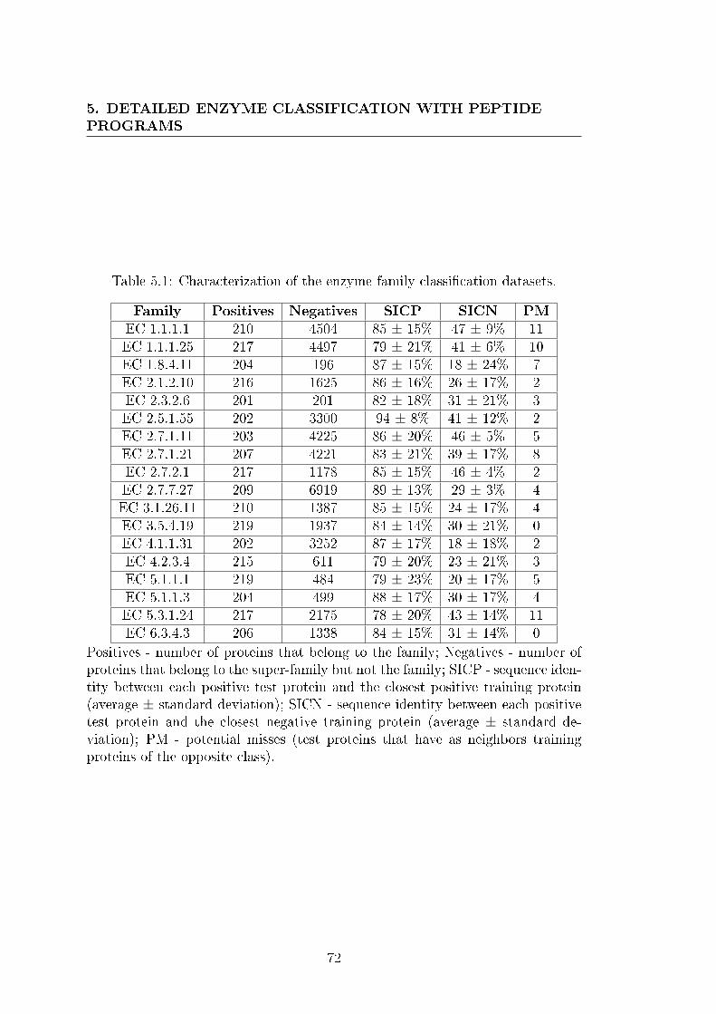
5. DETAILED ENZYME CLASSIFICATION WITH PEPTIDEPROGRAMS
Table 5.1: Characterization of the enzyme family classi�cation datasets.
Family Positives Negatives SICP SICN PMEC 1.1.1.1 210 4504 85 ± 15% 47 ± 9% 11EC 1.1.1.25 217 4497 79 ± 21% 41 ± 6% 10EC 1.8.4.11 204 196 87 ± 15% 18 ± 24% 7EC 2.1.2.10 216 1625 86 ± 16% 26 ± 17% 2EC 2.3.2.6 201 201 82 ± 18% 31 ± 21% 3EC 2.5.1.55 202 3300 94 ± 8% 41 ± 12% 2EC 2.7.1.11 203 4225 86 ± 20% 46 ± 5% 5EC 2.7.1.21 207 4221 83 ± 21% 39 ± 17% 8EC 2.7.2.1 217 1178 85 ± 15% 46 ± 4% 2EC 2.7.7.27 209 6919 89 ± 13% 29 ± 3% 4EC 3.1.26.11 210 1387 85 ± 15% 24 ± 17% 4EC 3.5.4.19 219 1937 84 ± 14% 30 ± 21% 0EC 4.1.1.31 202 3252 87 ± 17% 18 ± 18% 2EC 4.2.3.4 215 611 79 ± 20% 23 ± 21% 3EC 5.1.1.1 219 484 79 ± 23% 20 ± 17% 5EC 5.1.1.3 204 499 88 ± 17% 30 ± 17% 4EC 5.3.1.24 217 2175 78 ± 20% 43 ± 14% 11EC 6.3.4.3 206 1338 84 ± 15% 31 ± 14% 0
Positives - number of proteins that belong to the family; Negatives - number ofproteins that belong to the super-family but not the family; SICP - sequence iden-tity between each positive test protein and the closest positive training protein(average ± standard deviation); SICN - sequence identity between each positivetest protein and the closest negative training protein (average ± standard de-viation); PM - potential misses (test proteins that have as neighbors trainingproteins of the opposite class).
72
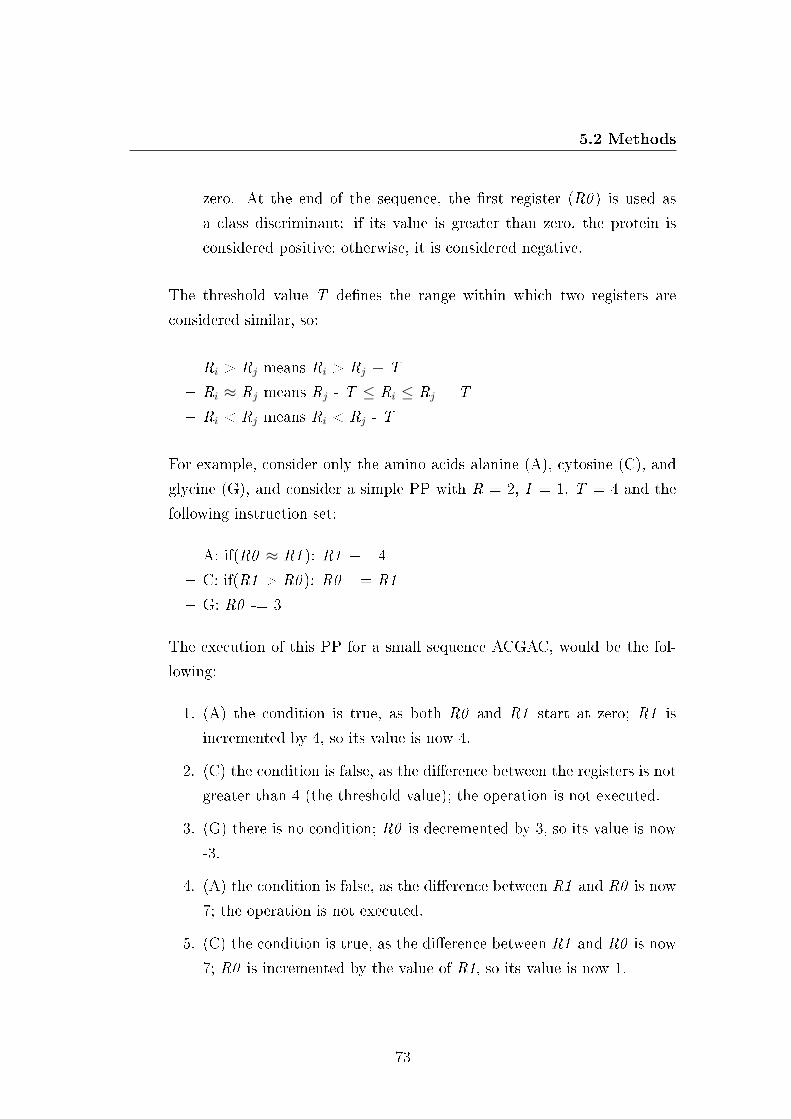
5.2 Methods
zero. At the end of the sequence, the �rst register (R0 ) is used as
a class discriminant: if its value is greater than zero, the protein is
considered positive; otherwise, it is considered negative.
The threshold value T de�nes the range within which two registers are
considered similar, so:
� Ri > Rj means Ri > Rj + T
� Ri ≈ Rj means Rj - T ≤ Ri ≤ Rj + T
� Ri < Rj means Ri < Rj - T
For example, consider only the amino acids alanine (A), cytosine (C), and
glycine (G), and consider a simple PP with R = 2, I = 1, T = 4 and the
following instruction set:
� A: if(R0 ≈ R1 ): R1 += 4
� C: if(R1 > R0 ): R0 += R1
� G: R0 -= 3
The execution of this PP for a small sequence ACGAC, would be the fol-
lowing:
1. (A) the condition is true, as both R0 and R1 start at zero; R1 is
incremented by 4, so its value is now 4.
2. (C) the condition is false, as the di�erence between the registers is not
greater than 4 (the threshold value); the operation is not executed.
3. (G) there is no condition; R0 is decremented by 3, so its value is now
-3.
4. (A) the condition is false, as the di�erence between R1 and R0 is now
7; the operation is not executed.
5. (C) the condition is true, as the di�erence between R1 and R0 is now
7; R0 is incremented by the value of R1, so its value is now 1.
73
5. DETAILED ENZYME CLASSIFICATION WITH PEPTIDEPROGRAMS
If this PP was trained for classi�cation, we would consider this protein as
a positive, because the �nal value of R0 is greater than zero.
The interesting aspect of this framework is that the e�ect of a given amino
acid depends on the state of the program, which means the program is able
to capture sequence patterns without comparing proteins directly.
5.2.3 Peptide Program Training
Training a PP classi�er requires selecting an instruction set such that the
�nal value of R0 for proteins that belong to the target class is greater than
zero, whereas its value for proteins that do not belong to that class is less
than or equal to zero. This is a combinatorial optimization problem, as the
objective is to search the instruction set space for the set that produces
the best classi�cation. However, an exhaustive search of the instruction set
space is unfeasible, as the number of possible sets for even a simple PP is
over 1079 (with R = 2, I = 1, T = 1). Thus, a metaheuristic procedure is
necessary to �nd an approximated solution in useful time.
In accordance with the original PP implementation by Falcao et al. (2008), I
opted for simulated annealing (Kirkpatrick et al., 1983) as the metaheuristic
to train PPs. Simulated annealing is a robust metaheuristic procedure
for combinatorial optimization that circumvents the local optima issue by
having a probability of accepting a worse solution. This probability is a
function of the di�erence between the new solution and the previous solution
and also of a state variable called temperature, which decreases as the
algorithm progresses. Initially, simulated annealing behaves more like a
random walk algorithm than an optimization algorithm, accepting most
new solutions, but as the temperature decreases it becomes gradually more
selective, and near the end behaves like a purely greedy algorithm.
I developed a multi-step training algorithm that consists of ten consecutive
steps of 15,000 iterations of simulated annealing. The temperature at the
beginning of the �rst nine steps is such that there is a 10% probability
of accepting a 10% worse solution, and it decreases exponentially on each
74
5.2 Methods
iteration so that by 12,000 iterations its e�ect is negligible (the probability
of accepting a 0.1% worse solution is only 0.0001%). In the last step the
temperature is zero, meaning that only better solutions are accepted. The
�rst step starts with an instruction set of randomly generated instructions,
whereas each other step starts with the best instruction set found thus
far. On each iteration, a neighbor solution is generated by changing one
of the instructions of one of the amino acids (selected at random) to a
new randomly generated instruction. This solution is then evaluated on
the training set, using the Matthews correlation coe�cient (MCC) as the
evaluation criterion, and the probability of it being accepted is computed.
Finally, the system randomly determines whether it is accepted or not,
taking the probability into account. The training process stops immediately
if a perfect training classi�cation (MCC = 1) is reached at any time.
5.2.4 Peptide Program Implementation and Develop-
ment
I implemented the PP methodology in the Java programming language,
to take advantage of the object-oriented paradigm to facilitate the devel-
opment of alternative frameworks. I created the interfaces Protein and
InstructionSet, and programmed the class PeptideProgram so that it works
with any implementation of those interfaces. The implementation of Protein
represents protein sequences, which in the case of the original PP frame-
work are simply arrays of integers (in the range [0-19]) to speed up PP
execution. The implementation of InstructionSet stores and updates the
instruction set and registers, including methods to generate a new random
instruction, to backup and rollback an instruction or the whole instruction
set, and to execute the instruction set on a given protein. In the original
PP framework, an instruction is stored as an array of 6 integers (3 to en-
code the condition and 3 to encode the operation) so the instruction set is a
multidimensional array of 20×I×6. The class PeptideProgram implements
the training algorithm, so that an instruction set can be trained as a PP
classi�er given arrays of positive and negative proteins. It also includes
75

5. DETAILED ENZYME CLASSIFICATION WITH PEPTIDEPROGRAMS
a method for testing the classi�er, given arrays of positive and negative
proteins.
I tested several combinations of PP parameters, verifying that R (number
of registers) and I (number of instructions per amino acid) strongly a�ected
the performance of the PPs, whereas N (register limit value), T (comparison
threshold) and S (register increment range) had little or no e�ect. The
reason for this is that R and I are the parameters that most determine the
amount of information a PP can encode, and consequently the dimension of
the solution space. By contrast N, T and S are essentially scale parameters,
and similar PPs can be obtained with di�erent values of these parameters
(S does a�ect the number of possible instructions, but much less than R).
As such, I chose �xed values for these three parameters, which were used
throughout my work: N=128, T=4 and S=8.
The e�ects of both R and I on PP performance are ambivalent. On the one
hand, increasing these parameters allows a PP to encode more information,
and thus to capture more complex sequence patterns. On the other hand,
this increases the dimension of the solution space which makes �nding a
near-optimum PP a more di�cult task. I tested the con�guration proposed
by Falcao et al. (2008) with R=8 and I=2, but veri�ed that the perfor-
mance of the PPs was generally better with a lower number of registers. I
determined that the optimum (default) con�guration for the detailed en-
zyme classi�cation problems was R=4 and I=2. However, in the evaluation
of the methodology I also tested a more complex con�guration with R=6
and a simpler con�guration with R=2 and I=1, in addition to the default
con�guration.
Since the PP training process is stochastic, multiple PPs should be trained
for each classi�cation problem to ensure good results. I initially trained
10 PPs per problem, but later concluded that 5 repetitions were su�cient,
since the training algorithm is reasonably robust. While there were cases
where the di�erence between two PPs trained for a given problem ranged
up to 10%, these cases were rare, and generally the di�erences were under
2%.
76

5.2 Methods
5.2.5 Alignment-Based Benchmark
To evaluate the performance of the PP methodology, I compared it to the
performance of alignment-based inference classi�ers, using the BLAST se-
quence alignment algorithm. This BLAST classi�cation consists on per-
forming a BLAST search for each test protein against the database of train-
ing proteins, and classifying it based on the classi�cation of the most similar
training protein(s) found. However, BLAST alignments are only consid-
ered signi�cant above a minimum similarity threshold (which depends on
the classi�cation problem) to ensure reliable classi�cation (Devos & Valen-
cia, 2000; Tian & Skolnick, 2003). As such, proteins that do not have any
alignments above this threshold are classi�ed as negatives by default.
To ensure the global quality of the sequence alignments, I used the rel-
ative BLAST score as the similarity metric. For a given alignment, the
relative BLAST score is given by the score of that alignment divided by
the score of the self-alignment of the query protein. Whereas the sequence
identity re�ects only local similarity, since it is relative to the aligned seg-
ment, the relative BLAST score is a measure of global similarity. I opted
for a minimum similarity threshold of 30%, which is widely considered the
minimum for reliable function prediction (Rost, 1999). Furthermore, my
study of the relationship between functional similarity and sequence simi-
larity (see Chapter 3) showed that below this threshold functional similar-
ity drops rapidly with sequence similarity, so function predictions based on
such alignments would be unreliable. Above this point, functional similar-
ity values are relatively high and increase slowly with sequence similarity,
so functional predictions are more reliable.
I tested two di�erent BLAST classi�cation algorithms: single-neighbor and
10% neighborhood. The di�erence between the two algorithms is that the
former looks only at the single most similar protein whereas the latter looks
at all proteins that are within 10% similarity of the most similar. The single-
neighbor algorithm corresponds to the most direct and common application
of BLAST for predicting protein function automatically, whereas the 10%
77

5. DETAILED ENZYME CLASSIFICATION WITH PEPTIDEPROGRAMS
neighborhood algorithm tries to mirror the type of analysis that a human
researcher might do when using BLAST in this context.
For each test protein in each classi�cation task, the 10% neighborhood
algorithm consists of the following steps:
� Perform a BLAST search against the database of training proteins for
that task.
� Compute the relative BLAST score of the highest scoring alignment.
� If the relative BLAST score is greater than 30%, retrieve the most
similar protein and all other proteins with alignments within 10% of the
most similar (and also above the 30% threshold). Otherwise, classify
the test protein as negative by default.
� Retrieve the class of each protein in the 10% neighborhood. If there
is at least 90% agreement between the proteins in the neighborhood,
then classify the test protein accordingly. Otherwise, leave the test
protein unclassi�ed.
The agreement of 90% required to classify a protein as positive is consistent
with the fact that, in case of doubt, it is preferable to leave a protein
unannotated than to make an erroneous annotation.
The single-neighbor algorithm is identical except that the size of the interval
is 0%. This means that the classi�cation is based on the single most similar
protein except in cases where there are multiple proteins with exactly equal
similarity.
5.2.6 Machine Learning Benchmark
In addition to comparing PPs with BLAST classi�ers, I also evaluated their
performance in comparison to a state of the art machine learning approach
for protein classi�cation. The machine learning methodology I selected
was the support vector machine (SVM) methodology, since it is by far
the most popular methodology used in this context (Ben-Hur & Weston,
78
5.2 Methods
2008; Han et al., 2006). I selected the popular sequence representation
consisting of the set of composition, transition and distribution descriptors
based on physicochemical properties of the amino acids as an additional
benchmark (Dubchak et al., 1995). In addition to its popularity, I opted
for this representation because it had been previously tested in enzyme
classi�cation, although only for predicting the more generic EC classes and
sub-classes (Cai et al., 2004; Han et al., 2004). This sequence representation
consists of 167 attributes, which are obtained as follows:
� The �rst 20 attributes are the fractions of each of the 20 amino acids
in the sequence.
� 7 physicochemical properties are considered: hydrophobicity, van der
Waals volume, polarity, polarizability, charge, secondary structure and
solvent accessibility.
� For each property, the amino acids are divided into 3 discrete classes,
according to their value for that property or probabilistically in the
case of secondary structure and solvent accessibility.
� For each of the 7 properties, each protein is converted from a sequence
of 20 amino acids into a sequence of 3-classes.
� For each of these sequences, the composition, transition and distribu-
tion descriptors are computed.
� There are 3 composition descriptors, corresponding to the fraction of
each of the 3 classes (for each property) in the sequence.
� There are 3 transition descriptors, which count the frequency with
which there are changes between the three classes along the sequence.
There are 3 attributes rather than 6 because the direction of the
changes is not taken into account (i.e. changes from A to B are grouped
together with changes from B to A).
� There are 15 distribution descriptors, which mark the distribution in
the sequence (position of the minimum, maximum and quartiles) of
each of the 3 classes.
79
5. DETAILED ENZYME CLASSIFICATION WITH PEPTIDEPROGRAMS
After transforming the protein sequences as described by Li et al. (2006),
I used the SVMlight implementation (Joachims, 1999) to train and test
property SVMs for each EC family. I trained and tested SVMs with the four
available types of kernels: linear, polynomyal, radial and sigmoid. I used
the default SVMlight parameters, since they enabled the perfect or near-
perfect classi�cation of all training instances with all kernel types. However,
to take into account the unbalance of the datasets, I set the weight of the
type I errors relative to the type II errors to the ratio between the number of
negatives and positives for each EC family. This ensures that the training is
not biased in the cases where the negatives largely outnumber the positives.
5.2.7 Evaluation Parameters
There are two kinds of errors a binary classi�er can make: type I and type
II errors. Type I errors are cases where the classi�er erroneously classi�es
negative instances as positive (false positives); whereas type II errors are
cases where it classi�es positive instances as negative (false negatives). In
protein classi�cation, type I errors are generally more important than type
II errors, since it is critical to avoid annotating proteins erroneously given
the risk of error propagation (Devos & Valencia, 2001). By contrast, not
annotating a protein that should have a given annotation has no signi�cant
consequences other than the waste of knowledge. Nevertheless, it is impor-
tant to account for type II errors to ensure that the classi�er is useful. For
instance, a classi�er that classi�es all instances as negative will make no
type I errors, but it is completely useless as a classi�er.
The parameters I used to evaluate classi�cation performance of are the
precision, the recall and the Matthews correlation coe�cient (MCC). Con-
sidering the confusion matrix of a binary classi�er, with true positives (TP),
true negatives (TN), false positives (FP) and false negatives (FN), they are
calculated by the following expressions:
Precision =TP
TP + FP(5.1)
80
5.3 Peptide Program Evaluation
Recall =TP
TP + FN(5.2)
MCC =TP × TN − FP × FN√
(TP + FP )(TP + FN)(TN + FP )(TN + FN)(5.3)
The precision measures how many of the instances classi�ed as positive
are true positives. It only accounts for type I errors, ranging from 0 when
there are no true positives, to 1 when there are no false positives. The
recall measures how many of the actual positive instances were classi�ed
as positive. It only accounts for type II errors, ranging from 0 when there
are no true positives, to 1 when there are no false negatives. The MCC is
generally considered a good measure of global classi�cation quality (Han
et al., 2006), as it accounts for both type I and type II errors, and also
accounts for the imbalance of the dataset. It ranges from -1 when the
classi�er is perfectly reversed (i.e. all positives are classi�ed as negative
and vice-versa) to 1 when the classi�er is perfect, taking the value of 0
when exactly half the positives and half the negatives are missclassi�ed
(i.e. the classi�er is completely random) or when either all positives or all
negatives are missclassi�ed (i.e. the classi�er is completely biased).
5.3 Peptide Program Evaluation
5.3.1 Peptide Program Classi�cation Results
For each of the 18 EC family classi�cation tasks, I trained and tested 10 PPs
with the default con�guration, and later 5 PPs with the simple con�guration
and another 5 PPs with the complex con�guration. I selected the PP with
the best training results per family, or in case of tie the one with the best
testing results. The default con�guration produced the best PP classi�ers
for all EC families except for two. Family EC 1.1.1.1 was better classi�ed
with the complex con�guration, whereas family EC 1.8.4.11 was perfectly
classi�ed with both the default and the simple con�gurations.
81
5. DETAILED ENZYME CLASSIFICATION WITH PEPTIDEPROGRAMS
The PP training results were perfect for 10 of the EC families, and had an
average precision of nearly 100%, an average recall of 97% and an average
MCC of 0.98 (Table 5.2). In terms of testing, the overall performance of the
PPs was good, with an average precision of 98%, an average recall of 94%
and an average MCC of 0.95. Five EC families were perfectly classi�ed in
testing, whereas �ve other families had relatively poor testing results (with
recall below 90%). Notably, the perfectly classi�ed families all had relatively
small datasets (below 1500 proteins) whereas the poorly classi�ed families
all had relatively large datasets (above 2000 proteins). This suggests that
PP performance was negatively a�ected by the size of the dataset, and
indeed there is a negative correlation coe�cient of -0.73 between the PP
testing MCC and the size of the datasets. However, it should be noted
that the precision of the PP classi�ers was generally high even for the EC
families with large datasets, with no classi�er having a precision below 93%.
5.3.2 BLAST Classi�cation Results
To evaluate the performance of the PPs, I applied the two BLAST clas-
si�cation algorithms to the 18 EC family classi�cation tasks. Note that
BLAST classi�cation does not encompass a training step, so there are no
training results. The test results of the two classi�cation algorithms were
nearly identical (Table 5.3). Both algorithms had an average precision of
99%, an average recall of 98% and an average MCC of 0.98. The only di�er-
ence between the two was that the single-neighbor algorithm had a higher
precision (but equal recall) for the families EC 1.8.4.11 and EC 5.3.1.24.
Overall, the performance of the BLAST classi�ers was very good, with per-
fect precision for most of the EC families and a very high recall for all but
two of them (EC 2.7.1.21 and EC 5.1.1.1). The families EC 1.1.1.1 and EC
2.7.1.21 proved more di�cult to classify than the others, as they were the
only families with both type I and type II errors from both algorithms.
82
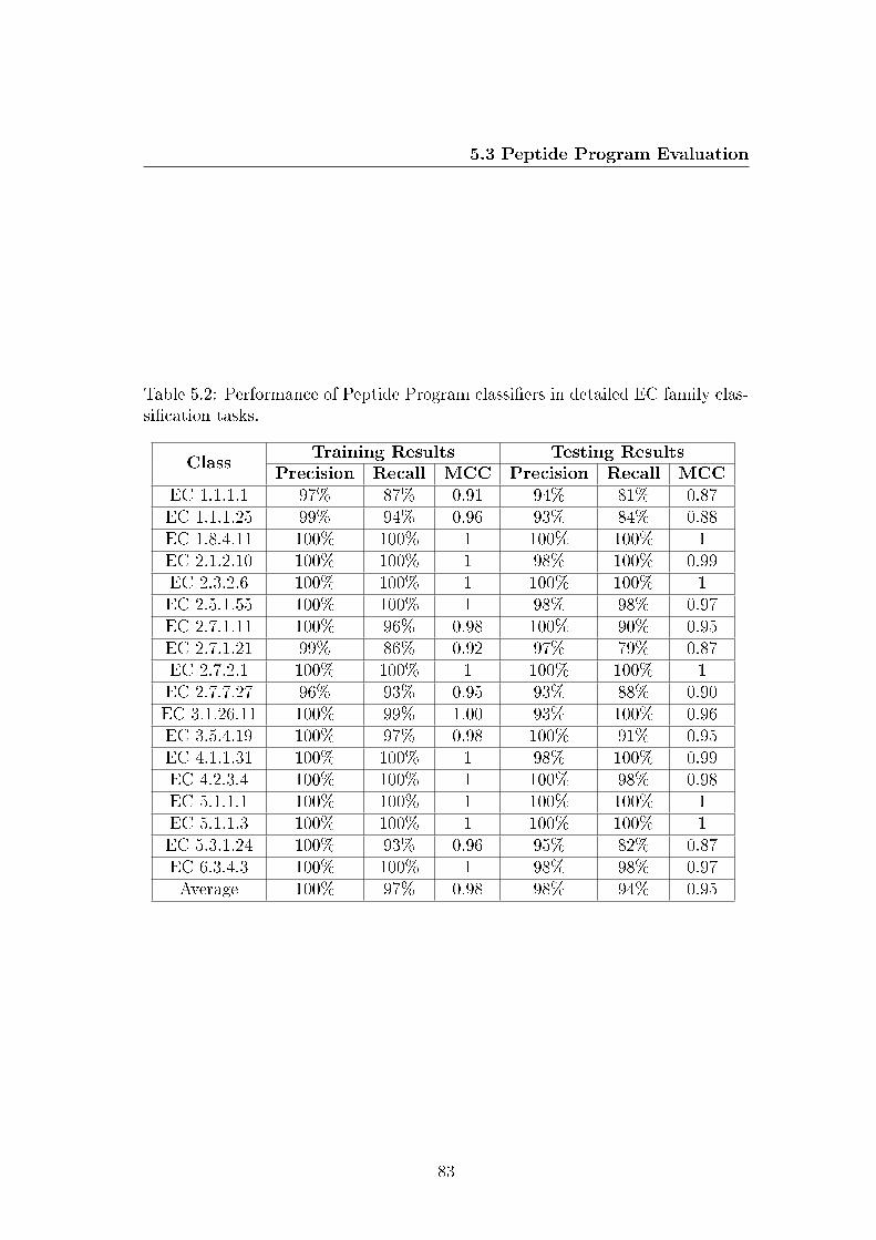
5.3 Peptide Program Evaluation
Table 5.2: Performance of Peptide Program classi�ers in detailed EC family clas-si�cation tasks.
ClassTraining Results Testing Results
Precision Recall MCC Precision Recall MCCEC 1.1.1.1 97% 87% 0.91 94% 81% 0.87EC 1.1.1.25 99% 94% 0.96 93% 84% 0.88EC 1.8.4.11 100% 100% 1 100% 100% 1EC 2.1.2.10 100% 100% 1 98% 100% 0.99EC 2.3.2.6 100% 100% 1 100% 100% 1EC 2.5.1.55 100% 100% 1 98% 98% 0.97EC 2.7.1.11 100% 96% 0.98 100% 90% 0.95EC 2.7.1.21 99% 86% 0.92 97% 79% 0.87EC 2.7.2.1 100% 100% 1 100% 100% 1EC 2.7.7.27 96% 93% 0.95 93% 88% 0.90EC 3.1.26.11 100% 99% 1.00 93% 100% 0.96EC 3.5.4.19 100% 97% 0.98 100% 91% 0.95EC 4.1.1.31 100% 100% 1 98% 100% 0.99EC 4.2.3.4 100% 100% 1 100% 98% 0.98EC 5.1.1.1 100% 100% 1 100% 100% 1EC 5.1.1.3 100% 100% 1 100% 100% 1EC 5.3.1.24 100% 93% 0.96 95% 82% 0.87EC 6.3.4.3 100% 100% 1 98% 98% 0.97Average 100% 97% 0.98 98% 94% 0.95
83
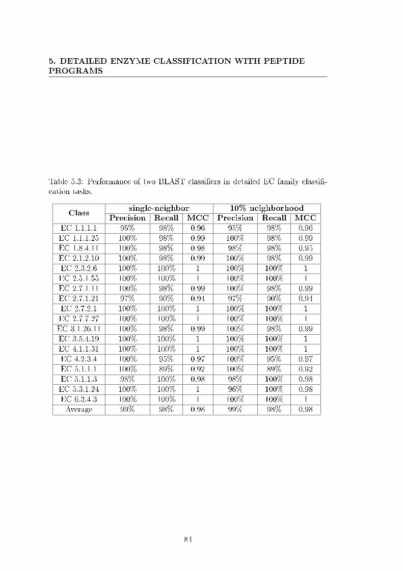
5. DETAILED ENZYME CLASSIFICATION WITH PEPTIDEPROGRAMS
Table 5.3: Performance of two BLAST classi�ers in detailed EC family classi�-cation tasks.
Classsingle-neighbor 10% neighborhood
Precision Recall MCC Precision Recall MCCEC 1.1.1.1 95% 98% 0.96 95% 98% 0.96EC 1.1.1.25 100% 98% 0.99 100% 98% 0.99EC 1.8.4.11 100% 98% 0.98 98% 98% 0.95EC 2.1.2.10 100% 98% 0.99 100% 98% 0.99EC 2.3.2.6 100% 100% 1 100% 100% 1EC 2.5.1.55 100% 100% 1 100% 100% 1EC 2.7.1.11 100% 98% 0.99 100% 98% 0.99EC 2.7.1.21 97% 90% 0.94 97% 90% 0.94EC 2.7.2.1 100% 100% 1 100% 100% 1EC 2.7.7.27 100% 100% 1 100% 100% 1EC 3.1.26.11 100% 98% 0.99 100% 98% 0.99EC 3.5.4.19 100% 100% 1 100% 100% 1EC 4.1.1.31 100% 100% 1 100% 100% 1EC 4.2.3.4 100% 95% 0.97 100% 95% 0.97EC 5.1.1.1 100% 89% 0.92 100% 89% 0.92EC 5.1.1.3 98% 100% 0.98 98% 100% 0.98EC 5.3.1.24 100% 100% 1 96% 100% 0.98EC 6.3.4.3 100% 100% 1 100% 100% 1Average 99% 98% 0.98 99% 98% 0.98
84

5.3 Peptide Program Evaluation
5.3.3 Property SVM Classi�cation Results
In addition to the BLAST classi�ers, I also applied the property SVM clas-
si�ers to the 18 EC family classi�cation tasks, to evaluate the performance
of the PPs. I tested SVM classi�ers with linear, polynomyal, radial and sig-
moid kernels. Both the polynomyal and sigmoid kernels produced perfect
training results for all EC families, but the polynomyal kernels produced the
best test results overall, so I opted for this type of kernel. The test results
of the property SVMs with polynomyal kernels were good overall, with an
average precision of 96%, and average recall of 97% and an average MCC
of 0.96 (Table 5.4). However, the precision of the property SVMs was often
lower than the recall, and it was mediocre for the families EC 1.1.1.1 and
5.1.1.3. While the worst SVM classi�ers also corresponded to EC families
with large datasets, the correlation between the MCC and the dataset size
was less meaningful than in the case of the PPs (-0.34).
5.3.4 Peptide Programs versus BLAST
In comparison with the BLAST classi�ers, the PPs had only a 1% lower
average precision but had a 4% lower average recall. However, the e�ect
of the dataset size on the PP performance was evident in the comparison
between the two methodologies. On the one hand, the PPs had better
results than the BLAST classi�ers for 4 of the 6 EC families with datasets
under 1500 proteins, and identical results for the other two families. On the
other hand, the PPs had clearly worse results than the BLAST classi�ers
for 11 of the 12 EC families with datasets over 1500 proteins, and similar
results for only family EC 2.1.2.10. The case of family EC 5.1.1.1, which
had the lowest recall with BLAST but was perfectly classi�ed with the
PPs, clearly shows that the PP methodology is not directly dependent upon
sequence similarity. Overall, the correlation between PP results and BLAST
results was low, with a correlation coe�cient between the MCC of both
methodologies of 0.13.
85
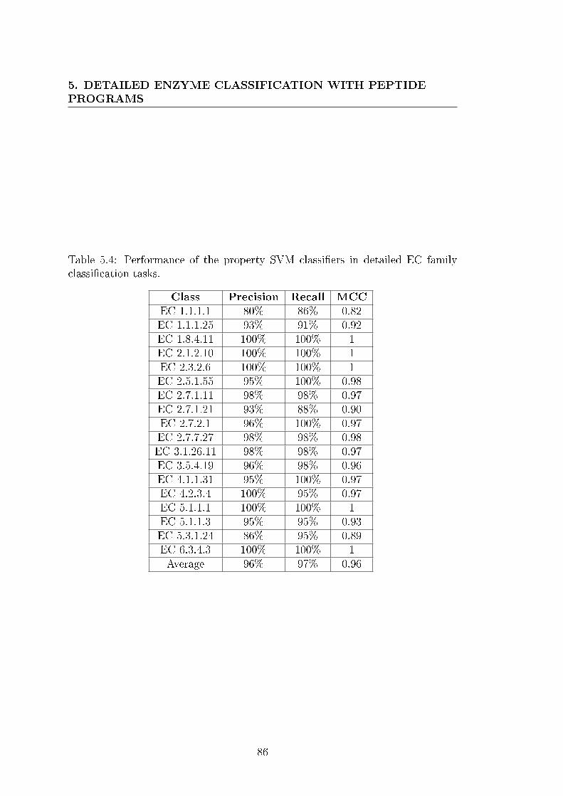
5. DETAILED ENZYME CLASSIFICATION WITH PEPTIDEPROGRAMS
Table 5.4: Performance of the property SVM classi�ers in detailed EC familyclassi�cation tasks.
Class Precision Recall MCCEC 1.1.1.1 80% 86% 0.82EC 1.1.1.25 93% 91% 0.92EC 1.8.4.11 100% 100% 1EC 2.1.2.10 100% 100% 1EC 2.3.2.6 100% 100% 1EC 2.5.1.55 95% 100% 0.98EC 2.7.1.11 98% 98% 0.97EC 2.7.1.21 93% 88% 0.90EC 2.7.2.1 96% 100% 0.97EC 2.7.7.27 98% 98% 0.98EC 3.1.26.11 98% 98% 0.97EC 3.5.4.19 96% 98% 0.96EC 4.1.1.31 95% 100% 0.97EC 4.2.3.4 100% 95% 0.97EC 5.1.1.1 100% 100% 1EC 5.1.1.3 95% 95% 0.93EC 5.3.1.24 86% 95% 0.89EC 6.3.4.3 100% 100% 1Average 96% 97% 0.96
86
5.4 Discussion
5.3.5 Peptide Programs versus Property SVMs
In comparison with the property SVMs, the PPs had a 2% higher average
precision but a 3% lower average recall. The PPs also outperformed the
SVMs on the EC families with small datasets, having better results for 3
of them and identical results for the other 3. Unlike the case of BLAST,
the PP and SVM results were well correlated, with a correlation coe�cient
between the MCC of the two methodologies of 0.74. In particular, the 4 EC
families which had the worst PP results also had the worst SVM results.
However, it was notable that the property SVMs often had a lower precision
than recall, whereas the opposite was true for the PPs. Overall, the PPs had
a higher precision than the SVMs for 10 EC families and a lower precision
for only 4 EC families.
5.4 Discussion
The premise behind the development of the PP methodology was that the
ability to deal directly with protein sequences could be advantageous for
predicting detailed function aspects of proteins, when compared with tra-
ditional machine learning methodologies. Furthermore, a machine learning
method suited for detailed function prediction could be an interesting al-
ternative to alignment-based approaches, if it was not directly dependent
upon sequence similarity.
Regarding the �rst premise, while the overall performance of the PPs was
not better than that of the property SVMs, they did have a higher average
precision, which is an important advantage in protein function prediction.
Given the risk of error propagation, it is less grave to leave a protein unan-
notated in case of doubt (i.e. make a type II error) than it is to make an
erroneous annotation (i.e. make a type I error), so precision is more im-
portant than recall. Since most EC classi�cation datasets were unbalanced,
having more negative test proteins than positive test proteins, misclassi�ed
negatives can be expected a priori to be more common than misclassi�ed
87
5. DETAILED ENZYME CLASSIFICATION WITH PEPTIDEPROGRAMS
positives. So, for an unbiased classi�er, the precision is expected to be
lower than the recall, as happens for the property SVMs. However, PPs
classify proteins by capturing complex but speci�c sequence patterns, and
so are biased classi�ers, much like alignment-based approaches. Even if a
negative test protein is very di�erent from all negative training proteins, it
is unlikely to match the pattern encoded by the PP, so it will tend to be
classi�ed as negative. Thus, the fact that the PPs had generally a higher
precision than recall, even for very unbalanced datasets, is an important
advantage of dealing directly with sequences.
There was also a drawback in dealing directly with sequences, as evidenced
by the negative correlation between classi�cation performance and dataset
size. In general, learning a model to classify a given dataset is more di�cult
the more diverse the dataset. However, diversity at the sequence level is
much greater than diversity at the property level, since di�erent amino acids
have identical property representations. Since small sequence variations are
common even between closely related proteins, in general, the larger the
dataset, the more diverse it will be at the sequence level, and the more
di�cult it will be to classify with a PP. This is not necessarily true at the
property level, as evidenced by the low correlation between classi�cation
performance and dataset size for the property SVMs. While the worst
results of the property SVM classi�ers did correspond to EC families with
large datasets, not all families will large datasets were poorly classi�ed with
this approach. For instance, the family EC 2.7.7.27, which has the largest
dataset, was well classi�ed with the property SVMs (MCC of 0.98) but
had poor results with the PPs (MCC of 0.90). Thus, dealing directly with
sequences has a signi�cant drawback, as it precludes the application of the
PP methodology to large classi�cation problems.
Another drawback of the PP methodology is the extensive training time.
It takes on average 2 seconds per protein to train a PP classi�er in a
CentOS Linux Server (with Quad-Core AMD Opteron Processor 2350 and
16GB RAM), ranging from 5 minutes for the EC families with the smallest
datasets to over 1 hour for the EC families with largest datasets. While
88

5.4 Discussion
executing a PP for a single protein is extremely fast, training a PP requires
executing it on each iteration of the training algorithm for each protein in
the training dataset, which corresponds to over 500 million executions for
the largest datasets. While the training time could undoubtedly be reduced
by further optimizing the algorithm and implementing it in a lower level
programming language, it cannot compete with the training time for SVMs,
which took under 1 minute for all EC families (including the time to pre-
process the datasets). Thus, this reinforces the fact that the applicability
of the PPs is limited to relatively small classi�cation problems, wherein the
quality of the results justi�es the training time.
I experimented with several simpler PP frameworks to determine if it was
possible to reduce the training time while retaining a higher precision than
the property SVMs. However, most simpli�ed frameworks led to a drop in
precision of at least 5%, even those with seemingly small modi�cations, such
as removing the conditions from the instructions. The only approach that
produced a high precision (97%) was using a reduced alphabet of 10 amino
acids (by grouping amino acids with similar properties), but this reduced
the training time only by 12%.
Regarding the second premise, it is evident from the overall quality of the
results and the drawback of the training time that the PP methodology can-
not compete with BLAST on large scale protein function prediction prob-
lems. However, the fact that the PPs surpassed the BLAST classi�ers on
the 6 EC classes with the smallest datasets demonstrates that despite being
based directly on protein sequences, the methodology is not directly depen-
dent upon sequence similarity. Thus, given the quality of the results, PPs
are an interesting approach for particular functional classi�cation problems
with under 1500 proteins.
It is likely that the PP methodology can also be adapted to DNA sequence
analysis problems, which are simpler than protein classi�cation problems
because DNA is a linear molecule and is composed by only 4 nucleotides.
89

Chapter 6
Exploring Sequence
Representations
6.1 Background
Traditional machine learning approaches cannot deal directly with protein
sequences, as they require data with a �xed number of attributes. Thus,
applying machine learning classi�ers to predict protein function typically
requires converting protein sequences into vectors of attributes that rep-
resent the sequence (Han et al., 2006; Ong et al., 2007). While several
sequence representations have been proposed for use with machine learning
classi�ers, most were employed only to predict generic functional aspects of
proteins, such as whether proteins bind DNA or whether they belong to a
given EC class or subclass (Cai et al., 2004; Garg & Gupta, 2008; Kumar
et al., 2007; Langlois et al., 2007; Liao et al., 2011). Likewise, the only
extensive study comparing the performance of multiple sequence represen-
tations was also evaluated on generic classi�cation problems (Ong et al.,
2007).
The development of the Peptide Program (PP) methodology showed that
there are advantages in dealing directly with protein sequences (see Chapter
5). However, the variability between proteins at the sequence level limits
91
6. EXPLORING SEQUENCE REPRESENTATIONS
this approach to relatively small classi�cation problems. While it is true
that transforming protein sequences into vectors of attributes implies a loss
of information, it is conceivable that a sequence representation could encode
su�cient information about the sequence to make reliable detailed protein
function predictions. Finding such a representation could expand the appli-
cability of machine learning approaches in the context of protein function
prediction, and potentially improve prediction quality in cases of divergent
evolution, in which alignment-based approaches typically fail (Whisstock &
Lesk, 2003).
In this chapter, I evaluate existing and novel vector representations of pro-
tein sequences in the context of detailed protein function prediction.
6.2 Methods
6.2.1 Datasets and Benchmarks
To evaluate the performance of the various sequence representations, I opted
for the set of 18 binary detailed enzyme classi�cation tasks previously used
to evaluate the PP methodology and described in Section 5.2.1. These
tasks consist in identifying whether a protein belongs to a given EC family,
knowing its EC sub-subclass.
6.2.2 Sequence Representations
One of the simplest representation of a protein sequence is its amino acid
composition, i.e. the frequency of each of the 20 amino acids in the se-
quence (Han et al., 2006; Ong et al., 2007). This representation encodes
no information about the sequence order and reduces sequences to vectors
of only 20 attributes. While I didn't expect this representation to be in
the least suited for detailed classi�cation, I tested it to determine the qual-
ity of classi�cation with minimal sequence information so as to be able to
determine the gain of more complex sequence representations.
92
6.2 Methods
In order to capture more information about the sequence, I conceived a sim-
ple variation of the amino acid composition representation. Rather than
measure the global amino acid composition of a protein sequence, I di-
vided the sequence into N equal parts and measured the local amino acid
compositions in each of those parts. This local amino acid composition
representation not only increases the number of attributes to N×20, butalso captures some information about the distribution of amino acids in the
sequence. I tested this representation with 2, 4, 6 and 8 parts. Despite the
simplicity of this approach, I found no publications reporting it.
Another simple strategy to capture more information about the sequence is
to measure the frequency of amino acids pairs (dipeptide composition) or
trios (tripeptide composition) (Jain et al., 2008; Liao et al., 2011; Mishra
et al., 2007; Ong et al., 2007). In both cases, overlapping N-peptide subse-
quences are typically considered, so a protein sequence with X amino acids
will have X-1 dipeptide subsequences and X-2 tripeptide subsequences. N-
peptide subsequences capture some information about the sequence order
at a local level, and as the length of the subsequences increases, may even
capture sequence patterns. However, the number of attributes increases
exponentially with the length of the subsequence (it is given by 20N) which
prevents the extension of this representation beyond tripeptides. Even the
tripeptide composition representation is already at risk from the curse of
dimensionality, as it comprises 8000 attributes. Given that the average pro-
tein sequence length is approximately 330 amino acids (as of the UniPro-
tKB release of January 2011) it is likely that some tripeptides may occur
only in a few proteins, particularly in small datasets. Thus, a classi�cation
model based on those tripeptides would be statistically unsound. However,
since the dipeptide composition representation encodes very little informa-
tion about the sequence order, I was interested in testing the tripeptide
composition representation, to test if the added information would improve
classi�cation quality.
I had previously tested a representation based on physicochemical prop-
erties in the evaluation of the PP methodology (see Section 5.2.6). This
93
6. EXPLORING SEQUENCE REPRESENTATIONS
representation is based on the descriptors composition, transition and dis-
tribution, which capture information about the physicochemical properties
of the amino acids at a local and global level. While there are other rep-
resentations based on correlations of physicochemical properties, I did not
explore them, since they reportedly do not di�er signi�cantly from the prop-
erty representation I had tested (Ong et al., 2007). Furthermore, I did not
expect that representations based on physicochemical properties could cap-
ture su�ciently speci�c sequence information for reliable detailed function
predictions.
6.2.3 Support Vector Machines
I tested the performance of the various sequence representations with the
support vector machine (SVM) methodology. I used the the SVMlight
implementation (Joachims, 1999) with polynomyal kernels and default pa-
rameters. However, to take into account the unbalance of the datasets, I
set the weight of the type I errors relative to the type II errors to the ratio
between the number of negatives and positives for each EC family. This en-
sures that the training is not biased in the cases where the negatives largely
outnumber the positives.
6.2.4 Vector Programs
In addition to the SVMs, I also tested the performance of some of the
sequence representations with a very simple PP framework designed for
linear classi�cation and based on vector sequence representations, which I
called Vector Programs (VPs):
� In the VP framework a protein is represented by a vector of attributes,
rather than by its sequence.
� The VP assigns to each attribute a �program� that corresponds simply
to an integer weight within a �xed range [-I,I ].
94
6.2 Methods
� For a given protein, the value of each attribute is multiplied by the
corresponding weight, and the resulting weighted sum of attributes is
the �nal score for that protein.
� Proteins that have a score greater than zero are classi�ed as positive,
whereas those that have a score smaller than or equal to zero are
classi�ed as negative.
� Training a VP consists of assigning weights to the attributes so as to
maximize classi�cation quality, which is a combinatorial optimization
program.
I implemented the VP framework in Java, within the PP package I had
implemented previously (see Section 5.2.4). Thus the VPs are trained with
the same simulated annealing algorithm used for training the PPs and de-
scribed in Section 5.2.3. Since the training process is stochastic, I trained 3
classi�ers per EC family with each sequence representation. I set the weight
limit at I=4.
6.2.5 Alignment-Based Benchmark
In order to evaluate the performance of the various sequence representa-
tions, I compared them with two BLAST classi�ers I had used previously
in the PP evaluation, which are described in Section 5.2.5. Since the aver-
age results of the single-neighbor BLAST classi�ers and 10% neighborhood
BLAST classi�ers were identical, I make no distinction between the two
algorithms.
6.2.6 Tripeptide-Based Similarity
Finally, I explored the possibility of using the tripeptide composition rep-
resentation for comparing protein sequences directly, as an alternative to
sequence alignment approaches. As a similarity measure, I employed the
Jaccard index, which is given by the ratio between the intersection and
95
6. EXPLORING SEQUENCE REPRESENTATIONS
the union of two sample sets. Thus, the resulting tripeptide-based measure
of similarity (TripSim) is simply given by the number of distinct tripep-
tide subsequences two proteins have in common, divided by the number of
distinct tripeptide subsequences they have combined.
I employed the TripSim measure in nearest-neighbors classi�cation, using
the same two classi�cation algorithms I had used with BLAST: single-
neighbor and 10% neighborhood. The algorithms were implemented exactly
as described for BLAST, except for the minimum similarity threshold (see
Section 5.2.5). Unlike the case of BLAST, I had no information to decide a
priori which would be a suitable minimum similarity threshold. Therefore,
I tested a range of thresholds, and based on the results determined that the
best threshold was 10%. Decreasing the threshold to 5% resulted in a lower
precision and recall, whereas increasing it to 15% led to a small increase in
precision but a large drop in recall.
6.2.7 Evaluation Parameters
The parameters I used to evaluate classi�cation performance were the pre-
cision, the recall and the Matthews correlation coe�cient (MCC), as de-
scribed in Section 5.2.7.
6.3 Testing Sequence Representations
6.3.1 Global and Local Amino Acid Composition
I tested the (global) amino acid composition representation with both SVM
classi�ers and VP classi�ers on the 18 EC family classi�cation tasks. As ex-
pected, classi�cation performance with this simple representation was poor,
with the composition SVMs having an average testing Matthews correla-
tion coe�cient (MCC) of 0.62 and the composition VPs having an average
testing MCC of 0.78, well below the average MCC of 0.98 of the BLAST
classi�ers (see Appendix B for the full results). The composition SVMs had
96
6.3 Testing Sequence Representations
a particularly poor performance, with all-negative classi�ers for 4 of the EC
families.
Dividing the sequence into 2 parts, to obtain the 2-part local amino acid
composition, increased classi�cation performance considerably. The 2-part
SVMs had a more reasonable average testing MCC of 0.84 and the 2-part
VPs also had a higher testing MCC of 0.89. Notably, the 2-part composi-
tion representation was su�ciently informative to enable the VP classi�ers
to classify perfectly the two EC families with the smallest datasets (EC
1.8.4.11 and 2.3.2.6). As expected, dividing the sequence into more parts
improved classi�cation performance further, but only until 6 parts, as shown
in Figure 6.1. The 8-part composition representations led to slightly worst
classi�cation results than the 6-part composition representation for both
SVMs and VPs. Overall, only one EC family was better classi�ed with
8-part SVMs than 6-part SVMs and none were better classi�ed with 8-part
VPs than with 6-part VPs (see Appendix B for the full results).
The 6-part SVMs had a slightly higher precision than the 6-part VPs (99%
versus 98%) but the two methodologies were nearly identical in recall (96%)
and MCC (0.97). Overall, both 6-part methodologies had a better perfor-
mance than the property SVMs (96% precision, 97% recall, 0.96 MCC) and
the PPs (98% precision, 94% recall, 0.95 MCC). Furthermore, their per-
formance was only slightly worst than that of the BLAST classi�ers (99%
precision, 98% recall, 0.98 MCC), and the 6-part SVMs actually matched
BLAST in average precision.
While overall the performance of the 6-part VPs was slightly worse than
that of the 6-part SVMs, they had an equal or better performance than the
6-part SVMs for all 9 EC families with datasets under 2000 proteins and
an equal or better performance than BLAST for 7 of those EC families.
Together with the PPs, the VPs were the best performing methodology on
relatively small datasets.
To assess the in�uence of the weight limit I in the 6-part VPs, I tested
the methodology with I=2 and I=8 for each EC family. As expected,
the smaller weight limit led to worse results (testing MCC of 0.94) since
97
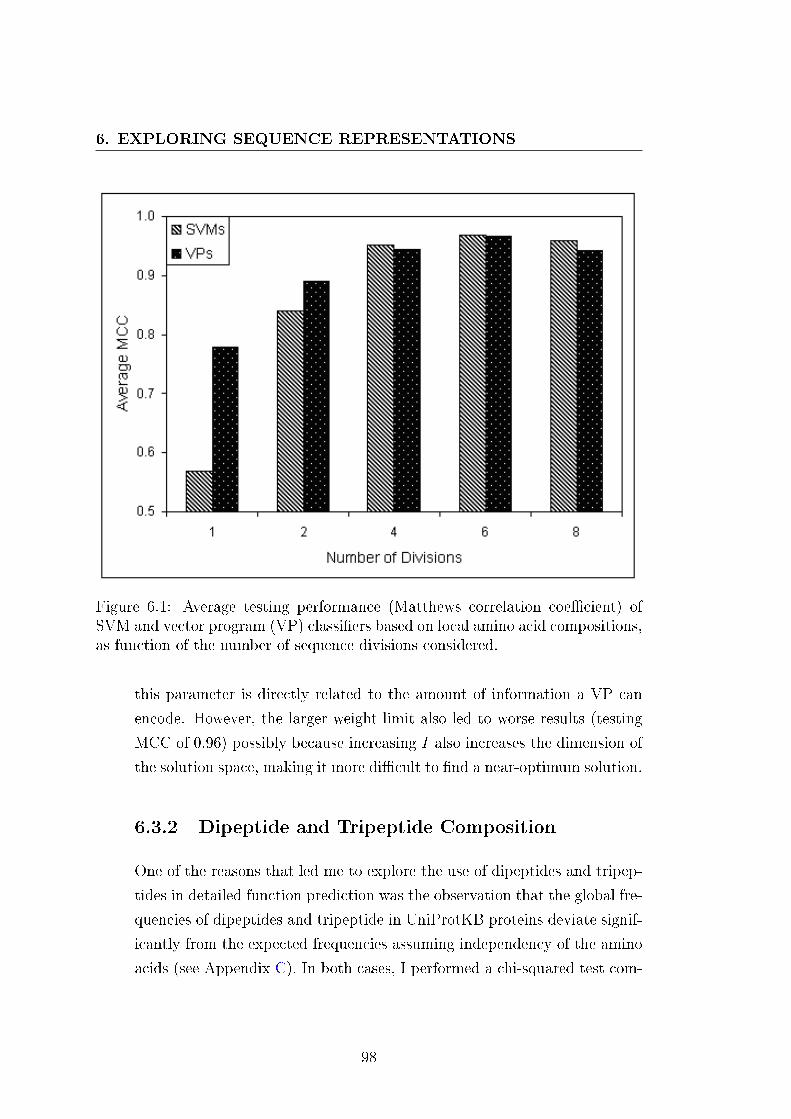
6. EXPLORING SEQUENCE REPRESENTATIONS
Figure 6.1: Average testing performance (Matthews correlation coe�cient) ofSVM and vector program (VP) classi�ers based on local amino acid compositions,as function of the number of sequence divisions considered.
this parameter is directly related to the amount of information a VP can
encode. However, the larger weight limit also led to worse results (testing
MCC of 0.96) possibly because increasing I also increases the dimension of
the solution space, making it more di�cult to �nd a near-optimum solution.
6.3.2 Dipeptide and Tripeptide Composition
One of the reasons that led me to explore the use of dipeptides and tripep-
tides in detailed function prediction was the observation that the global fre-
quencies of dipeptides and tripeptide in UniProtKB proteins deviate signif-
icantly from the expected frequencies assuming independency of the amino
acids (see Appendix C). In both cases, I performed a chi-squared test com-
98
6.3 Testing Sequence Representations
paring expected and observed frequencies, and obtained a p-value of zero,
which means that statistically, dipeptides and tripeptides are not collections
of independent amino acids. While it is evident that protein sequences are
not collections of independent amino acids, the fact that this is re�ected at
the level of dipeptides and tripeptides had not been previously reported.
It means that even local combinations of amino acids are under selective
pressures, and therefore are interesting attributes for protein classi�cation.
I evaluated the dipeptide composition and tripeptide composition represen-
tations only with the SVMmethodology, since the high number of attributes
of these representations would lead to an extensive VP training time (as it
is directly proportional to the number of attributes).
Both the dipeptide and the tripeptide SVMs had perfect training results
for all EC families. The testing results of the dipeptide SVMs were very
similar to those obtained with the 6-part SVMs, with an average precision
of 99%, an average recall of 96% and an average MCC of 0.97 (Table 6.1).
The tripeptide SVM results were even better, with an average precision of
100%, an average recall of 96% and an average MCC of 0.98. Notably, the
tripeptide SVMs had a higher average precision than the BLAST classi�ers
(100% versus 99%), having perfectly precise classi�ers for all EC families
except EC 1.1.1.1 (which also did not have perfect precision with BLAST).
Furthermore, while the recall of the tripeptide SVMs was inferior to that
of the BLAST classi�ers (96% versus 98%) the methodologies had a nearly
identical average MCC (0.98).
6.3.3 TripSim Classi�cation
To assess the possibility of using the tripeptide composition representation
directly to compare proteins, I conceived a simple tripeptide-based simi-
larity measure, called TripSim. I tested this measure in nearest-neighbors
classi�cation of the 18 EC families, employing the same two classi�cation
algorithms used with BLAST (single-neighbor and 10% neighborhood).
99
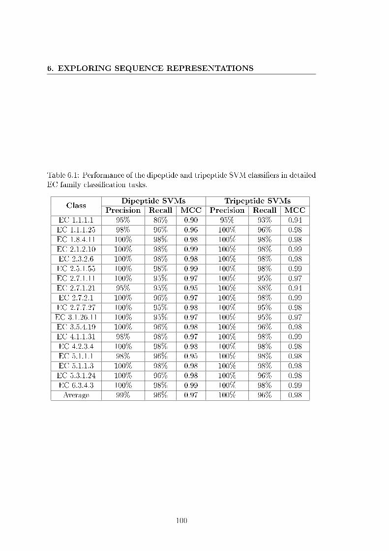
6. EXPLORING SEQUENCE REPRESENTATIONS
Table 6.1: Performance of the dipeptide and tripeptide SVM classi�ers in detailedEC family classi�cation tasks.
ClassDipeptide SVMs Tripeptide SVMs
Precision Recall MCC Precision Recall MCCEC 1.1.1.1 95% 86% 0.90 95% 93% 0.94EC 1.1.1.25 98% 96% 0.96 100% 96% 0.98EC 1.8.4.11 100% 98% 0.98 100% 98% 0.98EC 2.1.2.10 100% 98% 0.99 100% 98% 0.99EC 2.3.2.6 100% 98% 0.98 100% 98% 0.98EC 2.5.1.55 100% 98% 0.99 100% 98% 0.99EC 2.7.1.11 100% 95% 0.97 100% 95% 0.97EC 2.7.1.21 95% 95% 0.95 100% 88% 0.94EC 2.7.2.1 100% 96% 0.97 100% 98% 0.99EC 2.7.7.27 100% 95% 0.98 100% 95% 0.98EC 3.1.26.11 100% 95% 0.97 100% 95% 0.97EC 3.5.4.19 100% 96% 0.98 100% 96% 0.98EC 4.1.1.31 98% 98% 0.97 100% 98% 0.99EC 4.2.3.4 100% 98% 0.98 100% 98% 0.98EC 5.1.1.1 98% 96% 0.95 100% 98% 0.98EC 5.1.1.3 100% 98% 0.98 100% 98% 0.98EC 5.3.1.24 100% 96% 0.98 100% 96% 0.98EC 6.3.4.3 100% 98% 0.99 100% 98% 0.99Average 99% 96% 0.97 100% 96% 0.98
100
6.3 Testing Sequence Representations
The single-neighbor TripSim classi�ers were identical in performance to
the single-neighbor BLAST classi�ers, as both approaches had an average
precision of 99%, an average recall of 98%, and an average MCC of 0.98
(see Appendix B for the full results). Each approach had perfect classi�ers
for 8 EC families, and overall, their results were highly correlated, with a
correlation coe�cient of 0.86.
Unlike BLAST, which had a nearly identical performance with the single-
neighbor and 10% neighborhood algorithms, the 10% neighboorhood results
were noticeably worst than the single-neighbor TripSim results, with an
average precision of 98%, an average recall of 97% and an average MCC of
0.97. These results indicate that while the TripSim measure is identifying a
functionally-related single nearest neighbor as reliably as BLAST, it is less
reliable when looking at an extended neighborhood.
To further understand the relationship between TripSim and BLAST, I com-
pared the values of the two measures computed for all the 18 EC families.
Since there were over 11 million protein pairs, I plotted average TripSim
values over intervals of 1% relative BLAST score (Figure 6.2). The standard
deviation of the TripSim values per interval was around 5%, being slightly
lower for low BLAST values and slightly higher for high BLAST values.
It is notable that the TripSim and BLAST measures are well correlated, as
the average TripSim values increase monotonically with BLAST (excluding
a few outlier points for low BLAST values). The variation of TripSim
with BLAST has an approximately exponential behavior, as evidenced by
the reasonable �t of the exponential regression curve (Figure 6.2). This
means that the TripSim has a lower resolution than BLAST at low levels of
similarity, but a higher resolution at high levels of similarity, which suggests
that TripSim may actually be better than BLAST for comparing similar
proteins. However, it also indicates that TripSim is less suitable for �nding
distantly related proteins.
The outlier points in the �rst four BLAST intervals reveal a bias of the
TripSim measure for large proteins. Large proteins typically have a large
number of distinct tripeptides and thus are more likely to have tripeptides in
101
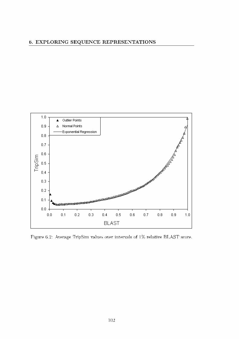
6. EXPLORING SEQUENCE REPRESENTATIONS
Figure 6.2: Average TripSim values over intervals of 1% relative BLAST score.
102
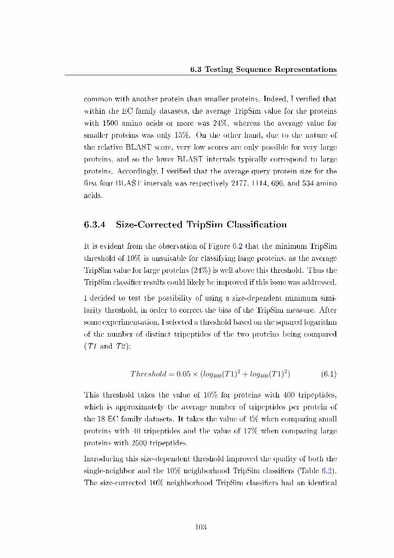
6.3 Testing Sequence Representations
common with another protein than smaller proteins. Indeed, I veri�ed that
within the EC family datasets, the average TripSim value for the proteins
with 1500 amino acids or more was 24%, whereas the average value for
smaller proteins was only 15%. On the other hand, due to the nature of
the relative BLAST score, very low scores are only possible for very large
proteins, and so the lower BLAST intervals typically correspond to large
proteins. Accordingly, I veri�ed that the average query protein size for the
�rst four BLAST intervals was respectively 2177, 1114, 696, and 534 amino
acids.
6.3.4 Size-Corrected TripSim Classi�cation
It is evident from the observation of Figure 6.2 that the minimum TripSim
threshold of 10% is unsuitable for classifying large proteins, as the average
TripSim value for large proteins (24%) is well above this threshold. Thus the
TripSim classi�er results could likely be improved if this issue was addressed.
I decided to test the possibility of using a size-dependent minimum simi-
larity threshold, in order to correct the bias of the TripSim measure. After
some experimentation, I selected a threshold based on the squared logarithm
of the number of distinct tripeptides of the two proteins being compared
(T1 and T2 ):
Threshold = 0.05× (log400(T1)2 + log400(T1)
2) (6.1)
This threshold takes the value of 10% for proteins with 400 tripeptides,
which is approximately the average number of tripeptides per protein of
the 18 EC family datasets. It takes the value of 4% when comparing small
proteins with 40 tripeptides and the value of 17% when comparing large
proteins with 2500 tripeptides.
Introducing this size-dependent threshold improved the quality of both the
single-neighbor and the 10% neighborhood TripSim classi�ers (Table 6.2).
The size-corrected 10% neighborhood TripSim classi�ers had an identical
103
6. EXPLORING SEQUENCE REPRESENTATIONS
performance to the 10% neighborhood BLAST classi�ers, as both measures
had an average precision of 99%, an average recall of 98% and an average
MCC of 0.98. The size-corrected single-neighbor TripSim classi�ers per-
formed better than the single-neighbor BLAST classi�ers, with a higher
average MCC of 0.99 and an increase in the number of perfectly classi�ed
EC families, to 10.
Table 6.2: Performance of two classi�ers based on the size-corrected TripSimmeasure in EC family classi�cation tasks.
Classsingle-neighbor 10% neighborhood
Precision Recall MCC Precision Recall MCCEC 1.1.1.1 95% 98% 0.96 95% 93% 0.94EC 1.1.1.25 100% 98% 0.99 95% 93% 0.94EC 1.8.4.11 100% 98% 0.98 100% 98% 0.98EC 2.1.2.10 100% 100% 1.00 100% 100% 1.00EC 2.3.2.6 100% 100% 1.00 100% 100% 1.00EC 2.5.1.55 100% 100% 1.00 100% 100% 1.00EC 2.7.1.11 100% 98% 0.99 100% 98% 0.99EC 2.7.1.21 97% 90% 0.94 97% 90% 0.94EC 2.7.2.1 100% 100% 1.00 98% 100% 0.99EC 2.7.7.27 100% 100% 1.00 100% 100% 1.00EC 3.1.26.11 100% 98% 0.99 100% 98% 0.99EC 3.5.4.19 100% 100% 1.00 100% 100% 1.00EC 4.1.1.31 100% 100% 1.00 100% 100% 1.00EC 4.2.3.4 100% 100% 1.00 100% 100% 1.00EC 5.1.1.1 100% 91% 0.93 100% 91% 0.93EC 5.1.1.3 98% 100% 0.98 98% 100% 0.98EC 5.3.1.24 100% 100% 1.00 90% 100% 0.94EC 6.3.4.3 100% 100% 1.00 100% 100% 1.00Average 99% 98% 0.99 99% 98% 0.98
6.4 Discussion
The main goal of this study was �nding vector representations of protein se-
quences that encoded su�cient information to enable machine learning clas-
104

6.4 Discussion
si�ers to make detailed protein function predictions as reliably as alignment-
based approaches.
While the performance of the classi�ers based on the amino acid compo-
sition representation was expectedly mediocre, the performance increased
substantially with the novel but simple local amino acid composition rep-
resentation. It was interesting to observe that while classi�er performance
increased up to 6 divisions, the quality of the 8-part classi�ers was slightly
inferior to that of the 6-part classi�ers. It is possible that the 8-part com-
position representation is already a�ected by the curse of dimensionality,
since more divisions means smaller divisions and less amino acids. Thus, as
the number of divisions increases some amino acids may only be present in
a given division on a few proteins, and not be statistically meaninful.
The fact that the 6-part VPs surpassed the performance of the PPs is
remarkable taking into consideration the relative simplicity of the two ap-
proaches. It is evident that the 6-part composition representation is less
informative than a full protein sequence, but this is compensated by the
fact that it is easier to model a group of proteins based on local amino acid
compositions than it is to model them based on global sequence patterns.
Thus, it is unsurprising that the 6-part VPs were less in�uenced by the size
of the datasets than the PPs. However, the fact that the 6-part VPs were
able to match the PPs in precision is surprising, and attest to the informa-
tiveness of the 6-part composition representation. Furthermore, the 6-part
VPs also matched the performance of the PPs on the EC families with small
datasets, surpassing all other methodologies tested. This suggests that, like
the PPs, the 6-part VPs are ideal for small classi�cation problems. The
6-part VPs also have a clear advantage over the PPs in terms of training
time, as training a 6-part VP takes at most 10% of the time it takes to train
a PP for the same dataset.
The 6-part SVMs had a better average performance than the 6-part VPs,
despite not performing as well for the EC families with small datasets.
Overall, they were able to compete with the BLAST classi�ers in precision,
and had an only slightly lower average MCC. The comparison between
105

6. EXPLORING SEQUENCE REPRESENTATIONS
the 6-part SVMs and property SVMs reveals that, despite a lower number
of attributes, the 6-part composition representation captures more speci�c
information about the sequence than the property representation, as it led
to a higher precision. However, the property representation led to a higher
recall, which suggests it is able to capture more distant relations between
proteins. Thus, the 6-part composition representation is more suitable for
predicting detailed functional aspects, whereas the property representation
is more suitable for predicting generic functional aspects.
The fact that the 6-part SVMs and dipeptide SVMs had identical results
also favors the 6-part composition representation, as the dipeptide composi-
tion representation has a much higher number of attributes. The implication
of these results is that 120 local amino acid frequencies are as informative
as 400 dipeptide frequencies, which strongly supports the novel local amino
acid composition representation.
The results obtained with the tripeptide SVMs surpassed those of all other
SVM approaches tested, as well as those of the PP and VP classi�ers. Re-
markably, the tripeptide SVMs surpassed even the BLAST classi�ers in
precision, with perfectly precise classi�ers for all EC families but one, and
matched the BLAST classi�ers in average MCC. This indicates that the
tripeptide composition representation captures highly speci�c information
about protein sequences. Furthermore, the comparison with the dipep-
tide SVMs suggests that tripeptides SVMs were not a�ected by the curse
of dimensionality, despite the high number of attributes of the tripeptide
composition representation. The tripeptide SVMs had both a higher testing
precision (by 0.6%) and a higher testing recall (by 0.3%) than the dipeptide
SVMs, which indicates that they did not over�t the training data any more
than the dipeptide SVMs did (as we would expect if there were cases of sta-
tistically unrepresentative attributes). Overall, the tripeptide SVMs had
the lowest standard deviation of all approaches tested regarding all three
evaluation parameters, which means it produced the most consistent results
in addition to the most precise. Based on these results, I can conclude that
106
6.4 Discussion
the main goal of this study was met, as the tripeptide composition rep-
resentation is indeed able to compete with alignment-based approaches in
detailed function prediction.
Led by the quality of the tripeptide SVM results, I decided to investigate
the possibility of using the tripeptide composition representation directly
to compare proteins, so as to fully assess the speci�city of the information
encoded by this representation. Considering the simplicity of the resulting
TripSim measure, the quality of the results obtained in nearest-neighbors
classi�cation was both surprising and remarkable. The fact that the Trip-
Sim classi�ers had similar or identical results to the BLAST classi�ers using
the same algorithm is a strong indicative that the tripeptide composition
representation encodes highly speci�c information about protein sequences.
This conclusion is reinforced by the strong (albeit non-linear) correlation
between TripSim and the relative BLAST score. The relationship between
the two similarity measures suggests that TripSim is more sensitive than
BLAST when comparing closely related proteins, but less sensitive when
comparing remotely related proteins. Thus, TripSim may be better than
BLAST for detailed protein classi�cation. Attesting to this conclusion was
the fact that, after correcting the TripSim threshold to account for large
proteins, the single-neighbor TripSim classi�ers performed better than the
single-neighbor BLAST classi�ers, having the highest average MCC of all
approaches tested. Additionally, considering that TripSim is computation-
ally much simpler than BLAST, it has the potential to at least speed up
databaset searches for similar proteins, when the alignment itself is not
needed.
107


Chapter 7
Predicting Molecular Function
Annotations
7.1 Background
My study of sequence representations showed that the tripeptide compo-
sition representation is su�ciently informative to enable reliable detailed
functional classi�cation of proteins, both when used with support vector
machine (SVM) classi�ers and when used directly to measure similarity for
nearest-neighbors classi�cation (see Chapter 6). However, the fact that both
tripeptide SVMs and TripSim classi�ers were able to compete with BLAST
classi�ers in binary classi�cation tasks, does not mean that they can chal-
lenge alignment-based approaches in practical protein function prediction
problems.
The main advantage of alignment-based approaches is that they can be
readily used on the full protein sequence and protein function space. Thus,
to challenge the alignment-based approaches, a protein function prediction
approach would have to be able to predict the complete Gene Ontology
(GO) molecular function annotations of a new protein sequence by compar-
ison with (or modelling of) all known proteins, within a few minutes.
109

7. PREDICTING MOLECULAR FUNCTION ANNOTATIONS
The TripSim measure can in principle emulate BLAST, and �nd similar
proteins by searching the full protein sequence space. However, it has to be
demonstrated whether it still is as reliable as BLAST at this scale, given
that my results only showed that it is as reliable as BLAST when dealing
with relatively small datasets of proteins, known a priori to be functionally
related.
As for the tripeptide SVMs, it is evident that they cannot be directly ap-
plied to the full protein sequence and function space, as they cannot deal
with data on this scale. The few applications of SVMs for general-purpose
annotation prediction have reduced the dimension of the problem by fo-
cusing on relatively small subsets of proteins and GO terms (Saraç et al.,
2010; Sokolov & Ben-Hur, 2010). Theoretically, it could also be possible to
have a hierarchical system of classi�ers that started by predicting generic
functional aspects and gradually increased the detail of the predictions.
However, with over 8000 molecular function terms (as of the GO release
of October 2010) and regular updates to the structure of GO, training and
maintaining such a system of classi�ers would be extremely di�cult.
My approach to this problem was to develop a hybrid classi�cation algo-
rithm, called TriGOPred that employs both a similarity search and tripep-
tide SVM classi�ers. First a similarity search is performed to �nd a local
group of potential solutions (and reduce the dimension of the problem);
then these solutions are modelled using tripeptide SVM classi�ers; and �-
nally these classi�ers are employed to predict the annotations of the query
protein. The premise behind this algorithm was that using tripeptide SVM
classi�ers instead of nearest-neighbors classi�ers should increase the relia-
bility of the predictions and reduce the impact of annotation errors.
In this chapter, I evaluate the performance of the TripSim measure and the
TriGOPred in a prediction task consisting on predicting the full molecular
function annotations of enzymes by analysis of the full UniProtKB.
110

7.2 Methods
7.2 Methods
7.2.1 Dataset
As a test set for GO molecular function annotation prediction, I selected
from the EC family datasets all proteins that had at least two annotations
based on experimental evidence to molecular function leaf terms, as of the
GOA release of January 2011. This criterion helps ensure that the proteins
are reliably annotated and have detailed annotations. From this selection,
I excluded proteins that had annotations to generic terms (less than 80%
descendent-based information content), to avoid incompletely annotated
proteins. I also excluded a protein that had no signi�cant BLAST hits
and another protein that had no signi�cant TripSim hits. I obtained a
testing dataset of 148 proteins with very detailed annotations based on
experimental evidence.
The training dataset, which is used as a database for similarity searches,
consists of all UniProtKB proteins with at least one molecular function
annotation and their GOA annotations (as of the January 2011 release of
both databases). For both BLAST and TripSim searches, the test protein
was excluded from the search results so that it didn't a�ect the predictions.
7.2.2 Evaluation Criteria
Evaluating GO annotation predictions is not straightforward since this is
a multi-class classi�cation problem and proteins typically belong to more
than one class. Thus, failing to predict an annotation out of four is obvi-
ously di�erent from failing to predict all four, and this should be taken into
account when evaluating predictions. Furthermore, not all GO terms are
equally informative, and failing to predict a generic term is evidently less
critical than failing to predict a very informative term. Thus, evaluating
GO annotation predictions is a matter of comparing the predicted annota-
tions with the real annotations, taking into account their informativeness,
111

7. PREDICTING MOLECULAR FUNCTION ANNOTATIONS
which can be done by calculating the semantic similarity between predicted
and real annotations.
Given the results of my evaluation of semantic similarity measures (see
Chapter 3), I selected the simGIC measure as the main evaluation criterion.
This measure is given by a weighted Jaccard index, so it accounts for both
type I and type II errors.
Since type I errors are more critical than type II errors in protein function
prediction, it is important to distinguish between the two types of errors. As
such, I also used as evaluation criterion a measure analogous to simGIC but
accounting only for type I errors, which is essentially a weighted precision.
This weighted precision is given by the sum of the information contents
of the correctly predicted terms, divided by the sum of the information
contents of all predicted terms.
7.2.3 BLAST Benchmark
There are several GO annotation prediction tools based on BLAST, which
use di�erent algorithms to process the BLAST results (Hawkins et al., 2009;
Saraç et al., 2010). Since my main goal was to assess whether TripSim
can match BLAST in capturing functionally related proteins, the choice
of algorithm was not critical, as long as the same algorithm was used with
both BLAST and TripSim. I adopted the scoring system proposed by Saraç
et al. (2010), but rather than a �xed number of neighbors, I opted for the
single-neighbor and 10% neighborhood algorithms I had used for EC family
classi�cation (see Section 5.2.5). I considered the same minimum similarity
threshold of 30%, but used the PSI-BLAST algorithm instead of BLASTP,
since it is more robust for low-similarity alignments (while identical for
high-similarity ones) and more commonly used in GO annotation prediction
tools.
For each test protein, the 10% neighborhood algorithm consists of the fol-
lowing steps:
112
7.2 Methods
� Perform a BLAST search against the database of all UniProtKB pro-
teins with molecular function annotations.
� Retrieve the protein with the highest scoring alignment, other than
the self-alignment of the test protein, and compute its relative BLAST
score.
� If the relative BLAST score is smaller than 30%, do not predict anno-
tations.
� Otherwise, retrieve the most similar protein and all other proteins with
alignments within 10% of the most similar (and also above the 30%
threshold).
� Retrieve a list of potential annotations consisting of all molecular func-
tion terms annotated to at least one of the neighbor proteins retrieved.
� For each term, ordered descendingly by information content, compute
its prediction score, given by the sum of the relative BLAST scores
of the proteins that are annotated to the term minus the sum of the
relative BLAST scores of the proteins that are not.
� If a term has a score greater than zero, it is attributed to the test
protein. To avoid redundant computations, all ancestors of the term
are automatically attributed to the test protein and removed from the
list of potential annotations.
The single-neighbor algorithm is identical except that the size of the interval
is 0%. This means that the classi�cation is based on the single most similar
protein except in cases where there are multiple proteins with exactly equal
similarity.
7.2.4 TripSim Nearest Neighbors
I tested TripSim with the same two prediction algorithms used for BLAST:
single-neighbor and 10% neighborhood. The only di�erence between the
TripSim algorithms and the BLAST algorithms was the minimum similarity
113
7. PREDICTING MOLECULAR FUNCTION ANNOTATIONS
threshold, which in the case of TripSim was the size-corrected minimum
similarity formula I used for EC family classi�cation (see Section 6.3.4).
7.2.5 TriGOPred Algorithm
While the TriGOPred algorithm can generically be applied with any simi-
larity search method, and with SVMs based on any sequence representation,
I conceived the algorithm to take advantage of the speci�city of the tripep-
tide composition representation. Thus, the intent of the algorithm is to
combine a TripSim search with tripeptide SVM classi�ers. However, I also
tested the algorithm with BLAST instead of TripSim.
For a given query protein, the TriGOPred algorithm consists of the following
steps:
� Perform a similarity search against the database of all UniProtKB
proteins with molecular function annotations, retrieving only proteins
above the size-dependent minimum similarity threshold.
� Retrieve all proteins from the similarity search results that are above
the minimum similarity threshold, up to a maximum of 200, to be used
as a training set.
� If the number of proteins in the training set is lower than 20, then
predict annotations using the 10% neighborhood algorithm.
� Otherwise, retrieve all molecular function terms annotated to all train-
ing proteins, to obtain a list of potential annotations.
� For each potential annotation, train a tripeptide SVM on the training
set, then run it for the query protein to predict whether it should be
annotated with the term.
� If an annotation is predicted, all ancestors of that term are automati-
cally attributed to it as well, and are removed from the list of potential
annotations to avoid redundant computations.
114
7.3 Evaluating TripSim and TriGOPred
The number of neighbors used to form the training set is limited to 200
to ensure a low computational time. I considered that 200 neighbors were
su�ciently representative of the local neighborhood of the protein to enable
reliable classi�cation. On the other hand, for proteins with less than 20
neighbors there is not enough information to justify training SVMs instead
of making predictions based on nearest-neighbors.
7.3 Evaluating TripSim and TriGOPred
7.3.1 BLAST Prediction Results
Applying the single-neighbor BLAST algorithm to the molecular function
annotation prediction dataset resulted in an average simGIC between pre-
dicted and real annotations of 52% and an average weighted precision of
98% (Table 7.1). This algorithm had predictions above 50% simGIC for 64
proteins, out of which 26 had perfect predictions (see Appendix D). It is
notable that the average number of hits considered for making predictions
was greater than 1, as several proteins in the dataset had multiple equally
distant neighbors.
The 10% neighborhood BLAST algorithm had a lower average simGIC
of 49%, but an identical weighted precision of 98%. This algorithm had
predictions above 50% simGIC for 58 proteins, out of which 17 had perfect
predictions.
7.3.2 TripSim Prediction Results
The performance of the single-neighbor TripSim predictors was identical to
that of the corresponding BLAST predictors, with an average simGIC of
52% and an average weighted precision of 98% (Table 7.1). There was one
more protein with predictions above 50% simGIC than with BLAST, but
the same number of proteins with perfect predictions (26). Individually,
the BLAST and TripSim predictions were identical for 93% of the proteins,
115
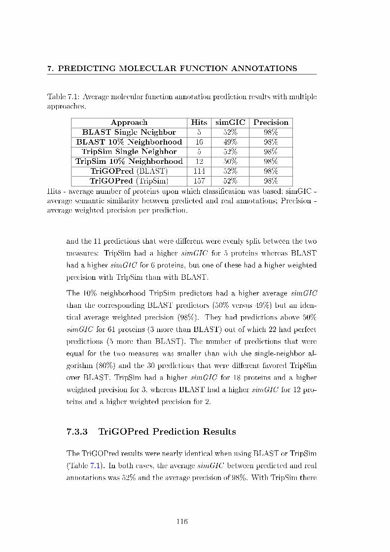
7. PREDICTING MOLECULAR FUNCTION ANNOTATIONS
Table 7.1: Average molecular function annotation prediction results with multipleapproaches.
Approach Hits simGIC PrecisionBLAST Single Neighbor 5 52% 98%
BLAST 10% Neighborhood 16 49% 98%TripSim Single Neighbor 5 52% 98%
TripSim 10% Neighborhood 12 50% 98%TriGOPred (BLAST) 114 52% 98%TriGOPred (TripSim) 157 52% 98%
Hits - average number of proteins upon which classi�cation was based; simGIC -average semantic similarity between predicted and real annotations; Precision -average weighted precision per prediction.
and the 11 predictions that were di�erent were evenly split between the two
measures: TripSim had a higher simGIC for 5 proteins whereas BLAST
had a higher simGIC for 6 proteins, but one of these had a higher weighted
precision with TripSim than with BLAST.
The 10% neighborhood TripSim predictors had a higher average simGIC
than the corresponding BLAST predictors (50% versus 49%) but an iden-
tical average weighted precision (98%). They had predictions above 50%
simGIC for 61 proteins (3 more than BLAST) out of which 22 had perfect
predictions (5 more than BLAST). The number of predictions that were
equal for the two measures was smaller than with the single-neighbor al-
gorithm (80%) and the 30 predictions that were di�erent favored TripSim
over BLAST. TripSim had a higher simGIC for 18 proteins and a higher
weighted precision for 3, whereas BLAST had a higher simGIC for 12 pro-
teins and a higher weighted precision for 2.
7.3.3 TriGOPred Prediction Results
The TriGOPred results were nearly identical when using BLAST or TripSim
(Table 7.1). In both cases, the average simGIC between predicted and real
annotations was 52% and the average precision of 98%. With TripSim there
116

7.3 Evaluating TripSim and TriGOPred
was one less protein with simGIC above 50% (63 versus 64) but two more
proteins with perfect predictions (25 versus 23). The TriGOPred results
were nearly identical to those obtained with the single-neighbor algorithm,
and better than those obtained with the 10% neighborhood algorithm, with
either BLAST or TripSim.
7.3.4 Comparison with Prediction Webtools
I tried to compare the performance of the results I obtained with those of
recent webtools for GO annotation prediction. I tested both PFP (Hawkins
et al., 2009) and GOPred (Saraç et al., 2010) on part of the molecular
function annotation dataset, but quickly realized that the comparison with
these webtools was unfair. PFP is not tuned to predict detailed annota-
tions, as its focus is on remotely related proteins. Thus, it had a simGIC
below 20% for each of the proteins I tested. GOPred did predict detailed
annotations in some cases, but being trained on a relatively small set of
GO terms, failed completely in other cases, leading to an average simGIC
of only 33% in 75 proteins tested (for which TriGOPred had an average
simGIC of 59%).
7.3.5 Discussion
It is interesting to note that the weighted precision of the predictions was
very high for all approaches tested, although the average simGIC was no-
tably lower. This means that there were few type I errors but several type
II errors, which is likely a consequence of the dataset selected. Since the
proteins selected all had detailed manually curated annotations, they are
likely to be annotated more completely and in more detail than most of
their homologues. Thus, predictions based on those homologues are likely
to lead to type II errors but not type I errors.
The results obtained with the TripSim measure con�rm that tripeptides
are su�ciently informative to measure sequence similarity, and can identify
117
7. PREDICTING MOLECULAR FUNCTION ANNOTATIONS
homologous proteins as reliably as BLAST. The fact that with the single-
neighbor algorithm 93% of the proteins had the same predictions with Trip-
Sim and BLAST indicates that the measures are nearly equivalent when it
comes to identifying the closest homologue. Furthermore, TripSim had a
slightly better performance than BLAST with the 10% neighborhood al-
gorithm, possibly because it was more selective (the average number of
neighbors considered with TripSim was lower than the average number of
neighbors considered with BLAST). This selectivity agrees with my previ-
ous observation that TripSim has a higher resolution than BLAST at high
similarity levels.
Overall, the quality of the results obtained with TripSim �rmly establishes
this measure as a viable alternative to BLAST in the context of protein
function prediction. Given that TripSim is computationally much simpler
than BLAST but leads to equivalent results, its adoption can signi�cantly
speed up database searches and function prediction tools. Indeed, a prelim-
inary implementation of TripSim in C takes only approximately 90 seconds
per protein to search the full UniProtKB database, whereas BLASTP takes
3-4 minutes, and PSI-BLAST takes 4-6 minutes (in a CentOS Linux Server
with Quad-Core AMD Opteron Processor 2350 and 16GB RAM).
The results obtained with TriGOPred clearly demonstrate that combin-
ing a similarity search with SVM classi�ers is a viable strategy for protein
function prediction. In principle, predictions based on a greater number
of proteins are less a�ected by annotation errors and less prone to prop-
agate them. Thus, TriGOPred should be preferred over nearest-neighbors
classi�ers considering that its results were otherwise identical or superior.
While there was no signi�cant di�erence between the TriGOPred results
based on TripSim and based on BLAST, the speed of TripSim improves the
applicability of TriGOPred, considering it requires training SVM classi�ers
on the �y. Using TripSim, the running time of TriGOPred is 2-5 minutes
(in the CentOS Linux Server mentioned above) which can compete with
most BLAST-based function prediction webtools. Thus, TriGOPred can be
of practical use for protein function prediction.
118

Chapter 8
Conclusions
Protein function prediction from sequence is a critical problem in genet-
ics and bioinformatics, as experimental methods for determining protein
functions are unable to keep up with the rate at which new sequences are
published.
The most common approaches to protein function prediction rely on se-
quence alignments and on the assumption that proteins of similar sequence
are homologues (i.e. have evolved from a common ancestor) and therefore
should perform similar or equal functions. The problem is that there are
both cases of proteins of similar function with very low or non-detectable
sequence similarity and cases of proteins of very similar sequence that have
evolved to perform di�erent functions. Thus, alignment-based approaches
are inherently limited, and it has been estimated that their generalized
use has led to the accumulation of errors in the functional annotation of
proteins.
Machine learning approaches not based on sequence alignments have also
been used in the context of protein function prediction. However, they have
mainly been applied to predict generic functional aspects of proteins, and
have generally been restricted to relatively small datasets. One limitation
of these approaches is the fact that they cannot deal directly with pro-
tein sequence data, and the loss of information resulting from transforming
119
8. CONCLUSIONS
sequences into vectors of features makes them less suitable for predicting
detailed functional aspects.
My thesis was that it is possible to extract su�cient information from pro-
tein sequences to make reliable detailed function predictions without the use
of sequence alignments, and therefore develop machine learning approaches
that could compete with alignment-based approaches for general-purpose
protein function prediction.
In a �rst step of my research work, I evaluated the use of semantic simi-
larity approaches to measure functional similarity between proteins, which
is essential to assess the quality of protein function predictions. I observed
that the average behavior of most of the semantic similarity approaches was
very similar, which indicated that these measures were all sensitive to the
same functional variations. However, some approaches were more sensitive
than others, and my evaluation identi�ed the simGIC measure as the most
sensitive overall. I employed this measure later in my research work, to
evaluate protein function predictions.
Additionally, I took advantage of the extensive data generated by this evalu-
ation to model the relationships between functional similarity and sequence
similarity, which was useful to understand the limits of alignment-based
protein function prediction. I observed that above 30% sequence similar-
ity, proteins have on average highly similar functions, and functional sim-
ilarity increases only slightly with sequence similarity. This means that
alignment-based protein function predictions above this sequence similarity
range should be reasonably reliable. However, not even 100% sequence simi-
larity is su�cient to ensure 100% semantic similarity. This may be partially
caused by cases of incomplete or inconsistent annotations, but also re�ects
the existence of cases of divergent evolution. Below 30% sequence simi-
larity, average function similarity values drop rapidly, which means that
alignment-based protein function predictions will generally be unreliable.
In addition to these qualitative observations, the function used to model
the relationships between functional similarity and sequence similarity can
120
be used to provide a con�dence score for alignment-based protein function
predictions taking into consideration the level of sequence similarity.
In a second step of my work, I analyzed the molecular function annotations
of proteins to assess their quality and consistency, focusing particularly on
electronic annotations. Inconsistent annotations are a major problem for
protein function prediction. If proteins that have the same function are not
consistently described with the same set of annotations, prediction meth-
ods will treat them as having di�erent functions, which will lead to even
more inconsistent annotations. I estimated with my analysis that 88% of
the sets of annotations used to describe protein functions are not univo-
cal descriptions, and that at least 20% of the proteins are inconsistently
annotated.
I also developed a novel data mining algorithm, based on association rule
learning, to �nd implicit relationships between molecular function terms,
with the goal of improving annotation consistency. The �rst version of this
algorithm was able to �nd 1,101 implicit relationships with an estimated
precision of 83%, whereas the second, more selective version of the algo-
rithm found 550 relationships with an estimated precision of 94%. This
high precision means it could potentially be used as an auxiliary tool to
increase the consistency of annotations predicted by protein function pre-
diction approaches.
Focusing now on protein function prediction, I developed and evaluated a
recently proposed machine learning methodology for protein classi�cation,
the Peptide Programs (PPs). The main innovation of PPs over traditional
machine learning methodologies is their ability to deal directly with protein
sequences and encode complex sequence patterns. My evaluation showed
that this innovation had both positive and negative aspects. On the one
hand, the sequence-speci�city of the PPs led to a consistently high precision
in detailed classi�cation tasks, surpassing state of the art machine learning
classi�ers and, in small problems, also alignment-based classi�ers. On the
other hand, the complexity of the solution space led to a noticeable drop in
classi�cation performance as the size of the datasets increased. Overall, my
121

8. CONCLUSIONS
conclusion was that PPs are an interesting approach for detailed functional
classi�cation problems of up to 1500 proteins. It is also possible that they
can be adapted to DNA sequence analysis problems, which are simpler than
protein classi�cation problems.
Following the evaluation of the PP methodology, I evaluated the perfor-
mance of multiple vector representations of protein sequences in detailed
classi�cation tasks. I tested these representations both with the established
support vector machine (SVM) methodology, and with a linear classi�cation
methodology based on the PP methodology and adapted to vector repre-
sentations, called Vector Programs (VP). One of the representations that
produced the best classi�cation results was the local amino acid composi-
tion representation, which I conceived. The SVM classi�ers based on this
representation were able to match the overall precision of alignment-based
classi�ers, and the VP classi�ers based on this representation had, together
with the PP methodology, the best results for small classi�cation problems.
However, these results were surpassed by the tripeptide composition rep-
resentation, as the SVM classi�ers based on this representation had the
highest precision of all approaches tested, being the most precise or tied for
most precise in all classi�cation tasks.
In addition to its application as an attribute set for SVM classi�ers, the
tripeptide composition representation was su�ciently informative to enable
the direct comparison of proteins. Indeed, I developed a tripeptide-based
measure of similarity, TripSim, which produced identical or slightly superior
results to those obtained with sequence alignments in detailed classi�cation
tasks, and later in a more di�cult molecular function annotation predic-
tion task. Considering that computing TripSim is simpler and faster than
computing a sequence alignment, it is a viable and interesting alternative
to sequence alignments in the context of protein function prediction.
To take advantage of the speed of the TripSim measure and the precision
of the SVMs based on the tripeptide composition representation, I con-
ceived a hybrid classi�cation algorithm called TriGOPred. One of the main
limitations of machine learning classi�ers is that, unlike alignment-based
122
approaches, they cannot be applied to the full protein space. My approach
to deal with this limitation was to reduce each function prediction problem
from the full protein space to a local neighborhood, by �rst employing a
similarity search method (in this case TripSim). The SVM classi�ers are
then used to model the local neighborhood rather than the full protein
space. Thus, the assumption behind this algorithm is that the solution for
the classi�cation problem is likely to lie within the local neighborhood, but
that using SVM classi�ers to �nd that solution is more reliable and more
robust than using a nearest-neighbors approach.
I evaluated the TriGOPred algorithm in the molecular function annotation
prediction task, where it matched or surpassed the performance of nearest-
neighbors classi�ers both based on sequence alignments and based on Trip-
Sim. While the TriGOPred results only matched the best nearest-neighbors
results, it should be noted that TriGOPred classi�cation was based on aver-
age on a much higher number of proteins. Therefore, TriGOPred should be
less a�ected by erroneously annotated proteins, and less prone to propagate
annotation errors than nearest-neighbors classi�ers. Additionally, thanks to
the speed of the TripSim measure, TriGOPred has a running time that can
compete with existing prediction tools, despite the fact that it requires
training SVM classi�ers on the �y.
123

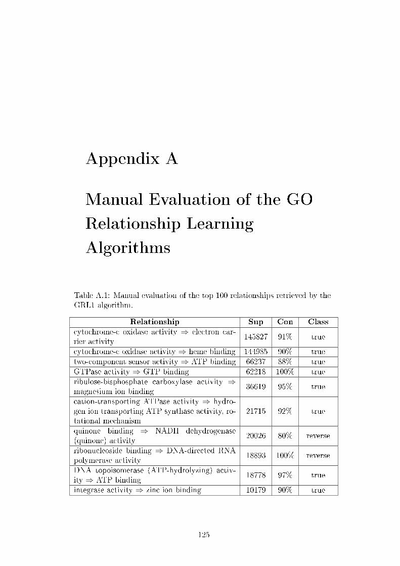
Appendix A
Manual Evaluation of the GO
Relationship Learning
Algorithms
Table A.1: Manual evaluation of the top 100 relationships retrieved by theGRL1 algorithm.
Relationship Sup Con Classcytochrome-c oxidase activity ⇒ electron car-rier activity
145827 91% true
cytochrome-c oxidase activity ⇒ heme binding 144985 90% truetwo-component sensor activity ⇒ ATP binding 66237 88% trueGTPase activity ⇒ GTP binding 62218 100% trueribulose-bisphosphate carboxylase activity ⇒magnesium ion binding
36619 95% true
cation-transporting ATPase activity ⇒ hydro-gen ion transporting ATP synthase activity, ro-tational mechanism
21715 92% true
quinone binding ⇒ NADH dehydrogenase(quinone) activity
20026 80% reverse
ribonucleoside binding ⇒ DNA-directed RNApolymerase activity
18893 100% reverse
DNA topoisomerase (ATP-hydrolyzing) activ-ity ⇒ ATP binding
18778 97% true
integrase activity ⇒ zinc ion binding 10179 90% true
125

A. MANUAL EVALUATION OF THE GO RELATIONSHIPLEARNING ALGORITHMS
Table A.1: (continued)
Relationship Sup Con Classglyceraldehyde-3-phosphate dehydrogenase(phosphorylating) activity ⇒ NAD or NADHbinding
10176 100% true
integrase activity ⇒ RNA-directed DNA poly-merase activity
9604 85% unknown
phosphopantetheine binding ⇒ acyl carrier ac-tivity
8433 100% reverse
1-aminocyclopropane-1-carboxylate synthaseactivity ⇒ pyridoxal phosphate binding
7101 100% true
phenylalanine-tRNA ligase activity ⇒ ATPbinding
6009 91% true
phenylalanine-tRNA ligase activity ⇒ tRNAbinding
5758 87% true
adenylate kinase activity ⇒ ATP binding 5514 99% trueaspartate-tRNA ligase activity⇒ ATP binding 4578 99% truetRNA dihydrouridine synthase activity⇒ FADbinding
4559 100% true
dihydrolipoyl dehydrogenase activity ⇒ FADbinding
4485 98% true
5-formyltetrahydrofolate cyclo-ligase activity⇒ATP binding
4427 100% true
four-way junction helicase activity ⇒ ATPbinding
4318 88% true
carbonate dehydratase activity⇒ zinc ion bind-ing
4126 88% true
phosphopyruvate hydratase activity ⇒ magne-sium ion binding
4104 99% true
glycine-tRNA ligase activity ⇒ ATP binding 4073 99% trueholo-[acyl-carrier-protein] synthase activity ⇒magnesium ion binding
4017 100% true
oxygen transporter activity ⇒ heme binding 4012 83% falsearginine-tRNA ligase activity ⇒ ATP binding 4005 99% trueoxygen transporter activity ⇒ oxygen binding 4002 83% truecysteine synthase activity ⇒ pyridoxal phos-phate binding
4001 100% true
copper-exporting ATPase activity⇒ATP bind-ing
3993 99% true
126
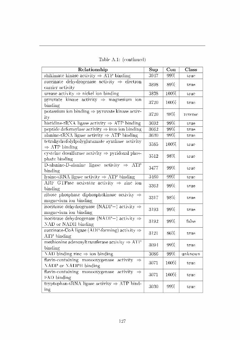
Table A.1: (continued)
Relationship Sup Con Classshikimate kinase activity ⇒ ATP binding 3947 99% truesuccinate dehydrogenase activity ⇒ electroncarrier activity
3898 89% true
urease activity ⇒ nickel ion binding 3838 100% truepyruvate kinase activity ⇒ magnesium ionbinding
3720 100% true
potassium ion binding⇒ pyruvate kinase activ-ity
3720 98% reverse
histidine-tRNA ligase activity ⇒ ATP binding 3692 99% truepeptide deformylase activity⇒ iron ion binding 3662 99% truealanine-tRNA ligase activity ⇒ ATP binding 3630 99% truetetrahydrofolylpolyglutamate synthase activity⇒ ATP binding
3585 100% true
cysteine desulfurase activity ⇒ pyridoxal phos-phate binding
3512 98% true
D-alanine-D-alanine ligase activity ⇒ ATPbinding
3477 99% true
lysine-tRNA ligase activity ⇒ ATP binding 3460 99% trueARF GTPase activator activity ⇒ zinc ionbinding
3362 99% true
ribose phosphate diphosphokinase activity ⇒magnesium ion binding
3317 98% true
isocitrate dehydrogenase (NADP+) activity ⇒magnesium ion binding
3193 99% true
isocitrate dehydrogenase (NADP+) activity ⇒NAD or NADH binding
3192 99% false
succinate-CoA ligase (ADP-forming) activity⇒ATP binding
3121 86% true
methionine adenosyltransferase activity⇒ATPbinding
3094 99% true
NAD binding zinc ⇒ ion binding 3086 99% unknown�avin-containing monooxygenase activity ⇒NADP or NADPH binding
3071 100% true
�avin-containing monooxygenase activity ⇒FAD binding
3071 100% true
tryptophan-tRNA ligase activity ⇒ ATP bind-ing
3030 99% true
127
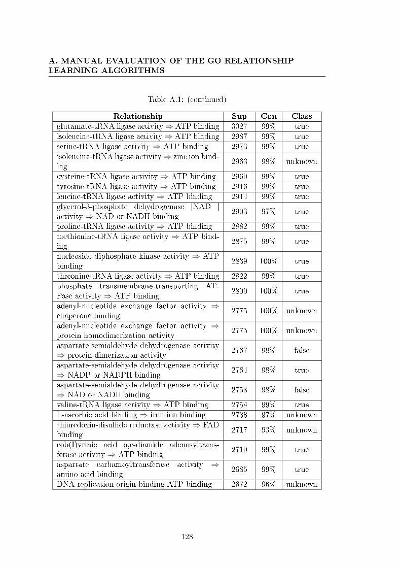
A. MANUAL EVALUATION OF THE GO RELATIONSHIPLEARNING ALGORITHMS
Table A.1: (continued)
Relationship Sup Con Classglutamate-tRNA ligase activity⇒ ATP binding 3027 99% trueisoleucine-tRNA ligase activity⇒ ATP binding 2987 99% trueserine-tRNA ligase activity ⇒ ATP binding 2973 99% trueisoleucine-tRNA ligase activity⇒ zinc ion bind-ing
2963 98% unknown
cysteine-tRNA ligase activity ⇒ ATP binding 2960 99% truetyrosine-tRNA ligase activity ⇒ ATP binding 2916 99% trueleucine-tRNA ligase activity ⇒ ATP binding 2914 99% trueglycerol-3-phosphate dehydrogenase [NAD+]activity ⇒ NAD or NADH binding
2903 97% true
proline-tRNA ligase activity ⇒ ATP binding 2882 99% truemethionine-tRNA ligase activity ⇒ ATP bind-ing
2875 99% true
nucleoside diphosphate kinase activity ⇒ ATPbinding
2839 100% true
threonine-tRNA ligase activity⇒ ATP binding 2822 99% truephosphate transmembrane-transporting AT-Pase activity ⇒ ATP binding
2800 100% true
adenyl-nucleotide exchange factor activity ⇒chaperone binding
2775 100% unknown
adenyl-nucleotide exchange factor activity ⇒protein homodimerization activity
2775 100% unknown
aspartate-semialdehyde dehydrogenase activity⇒ protein dimerization activity
2767 98% false
aspartate-semialdehyde dehydrogenase activity⇒ NADP or NADPH binding
2764 98% true
aspartate-semialdehyde dehydrogenase activity⇒ NAD or NADH binding
2758 98% false
valine-tRNA ligase activity ⇒ ATP binding 2754 99% trueL-ascorbic acid binding ⇒ iron ion binding 2738 97% unknownthioredoxin-disul�de reductase activity⇒ FADbinding
2717 93% unknown
cob(I)yrinic acid a,c-diamide adenosyltrans-ferase activity ⇒ ATP binding
2710 99% true
aspartate carbamoyltransferase activity ⇒amino acid binding
2685 99% true
DNA replication origin binding ATP binding 2672 96% unknown
128
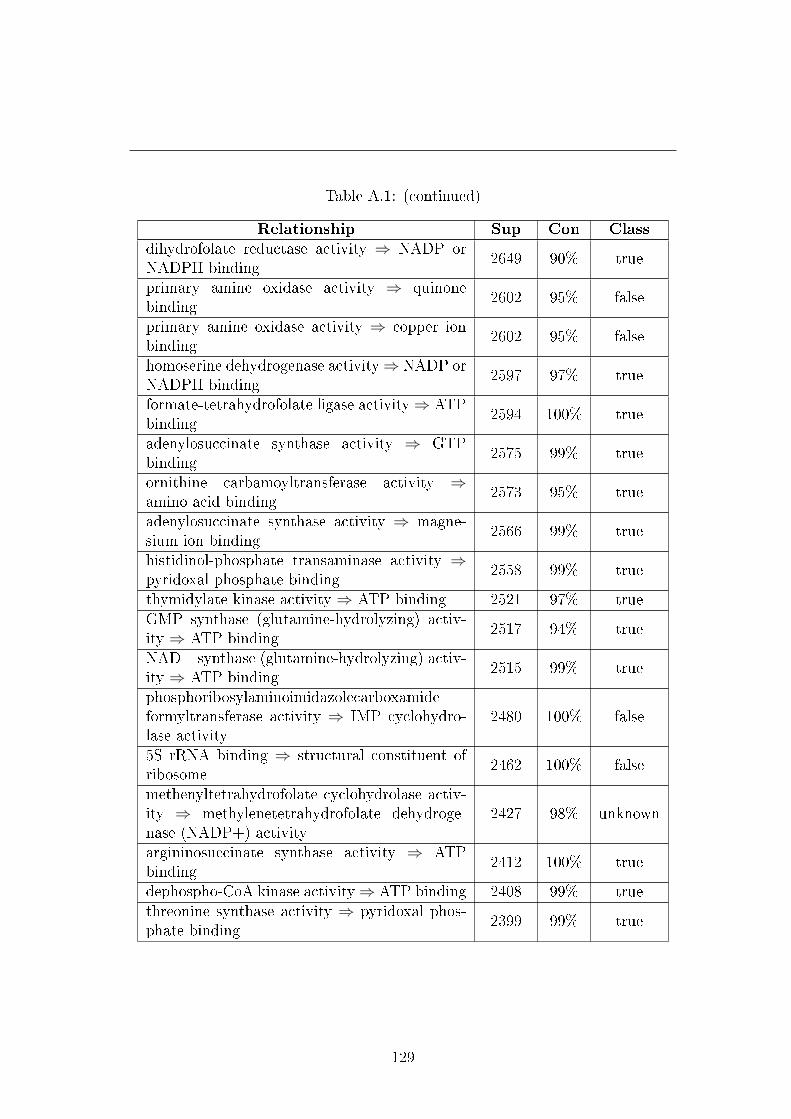
Table A.1: (continued)
Relationship Sup Con Classdihydrofolate reductase activity ⇒ NADP orNADPH binding
2649 90% true
primary amine oxidase activity ⇒ quinonebinding
2602 95% false
primary amine oxidase activity ⇒ copper ionbinding
2602 95% false
homoserine dehydrogenase activity⇒ NADP orNADPH binding
2597 97% true
formate-tetrahydrofolate ligase activity⇒ ATPbinding
2594 100% true
adenylosuccinate synthase activity ⇒ GTPbinding
2575 99% true
ornithine carbamoyltransferase activity ⇒amino acid binding
2573 95% true
adenylosuccinate synthase activity ⇒ magne-sium ion binding
2566 99% true
histidinol-phosphate transaminase activity ⇒pyridoxal phosphate binding
2558 99% true
thymidylate kinase activity ⇒ ATP binding 2521 97% trueGMP synthase (glutamine-hydrolyzing) activ-ity ⇒ ATP binding
2517 94% true
NAD+ synthase (glutamine-hydrolyzing) activ-ity ⇒ ATP binding
2515 99% true
phosphoribosylaminoimidazolecarboxamideformyltransferase activity ⇒ IMP cyclohydro-lase activity
2480 100% false
5S rRNA binding ⇒ structural constituent ofribosome
2462 100% false
methenyltetrahydrofolate cyclohydrolase activ-ity ⇒ methylenetetrahydrofolate dehydroge-nase (NADP+) activity
2427 98% unknown
argininosuccinate synthase activity ⇒ ATPbinding
2412 100% true
dephospho-CoA kinase activity⇒ ATP binding 2408 99% truethreonine synthase activity ⇒ pyridoxal phos-phate binding
2399 99% true
129

A. MANUAL EVALUATION OF THE GO RELATIONSHIPLEARNING ALGORITHMS
Table A.1: (continued)
Relationship Sup Con Classphosphoribosylamine-glycine ligase activity ⇒ATP binding
2385 98% true
phosphoribosylaminoimidazolesuccino-carboxamide synthase activity ⇒ ATPbinding
2369 96% true
UDP-N-acetylmuramoylalanyl-D-glutamyl-2,6-diaminopimelate-D-alanyl-D-alanine ligaseactivity ⇒ ATP binding
2290 100% true
L-threonine ammonia-lyase activity ⇒ pyri-doxal phosphate binding
2269 98% true
[formate-C-acetyltransferase]-activating en-zyme activity ⇒ 4 iron, 4 sulfur clusterbinding
2269 95% true
Sup - Support, Con - Con�dence, Class - Classi�cation.
Table A.2: Manual evaluation of the top 100 relationships retrieved by theGRL2 algorithm.
Relationship Sup Con Agr ClassGTPase activity ⇒ GTP binding 62218 100% 95% trueribonucleoside binding ⇒ DNA-directedRNA polymerase activity
18893 100% 100% reverse
DNA topoisomerase (ATP-hydrolyzing)⇒ ATP binding
18778 97% 82% true
phosphopantetheine binding ⇒ acyl car-rier activity
8433 100% 94% reverse
1-aminocyclopropane-1-carboxylate syn-thase ⇒ pyridoxal phosphate binding
7101 100% 97% true
adenylate kinase ⇒ ATP binding 5514 99% 86% truetRNA dihydrouridine synthase ⇒ FADbinding
4559 100% 100% true
5-formyltetrahydrofolate cyclo-ligase ⇒ATP binding
4427 100% 94% true
glycine-tRNA ligase ⇒ ATP binding 4073 99% 88% trueholo-[acyl-carrier-protein] synthase ⇒magnesium ion binding
4017 100% 89% true
arginine-tRNA ligase ⇒ ATP binding 4005 99% 88% true
130
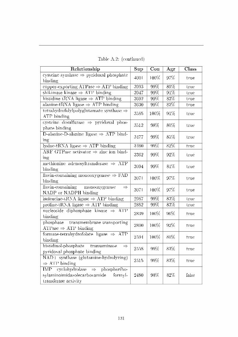
Table A.2: (continued)
Relationship Sup Con Agr Classcysteine synthase ⇒ pyridoxal phosphatebinding
4001 100% 97% true
copper-exporting ATPase⇒ ATP binding 3993 99% 89% trueshikimate kinase ⇒ ATP binding 3947 99% 91% truehistidine-tRNA ligase ⇒ ATP binding 3692 99% 83% truealanine-tRNA ligase ⇒ ATP binding 3630 99% 82% truetetrahydrofolylpolyglutamate synthase ⇒ATP binding
3585 100% 91% true
cysteine desulfurase ⇒ pyridoxal phos-phate binding
3512 98% 80% true
D-alanine-D-alanine ligase ⇒ ATP bind-ing
3477 99% 85% true
lysine-tRNA ligase ⇒ ATP binding 3460 99% 82% trueARF GTPase activator ⇒ zinc ion bind-ing
3362 99% 92% true
methionine adenosyltransferase ⇒ ATPbinding
3094 99% 81% true
�avin-containing monooxygenase ⇒ FADbinding
3071 100% 97% true
�avin-containing monooxygenase ⇒NADP or NADPH binding
3071 100% 97% true
isoleucine-tRNA ligase ⇒ ATP binding 2987 99% 83% trueproline-tRNA ligase ⇒ ATP binding 2882 99% 83% truenucleoside diphosphate kinase ⇒ ATPbinding
2839 100% 96% true
phosphate transmembrane-transportingATPase ⇒ ATP binding
2800 100% 92% true
formate-tetrahydrofolate ligase ⇒ ATPbinding
2594 100% 80% true
histidinol-phosphate transaminase ⇒pyridoxal phosphate binding
2558 99% 83% true
NAD+ synthase (glutamine-hydrolyzing)⇒ ATP binding
2515 99% 83% true
IMP cyclohydrolase ⇒ phosphoribo-sylaminoimidazolecarboxamide formyl-transferase activity
2480 98% 82% false
131
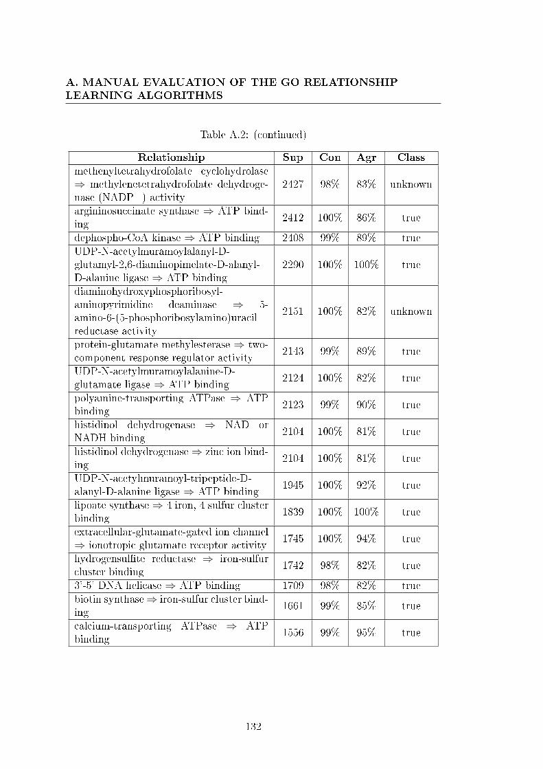
A. MANUAL EVALUATION OF THE GO RELATIONSHIPLEARNING ALGORITHMS
Table A.2: (continued)
Relationship Sup Con Agr Classmethenyltetrahydrofolate cyclohydrolase⇒ methylenetetrahydrofolate dehydroge-nase (NADP+) activity
2427 98% 83% unknown
argininosuccinate synthase ⇒ ATP bind-ing
2412 100% 86% true
dephospho-CoA kinase ⇒ ATP binding 2408 99% 89% trueUDP-N-acetylmuramoylalanyl-D-glutamyl-2,6-diaminopimelate-D-alanyl-D-alanine ligase ⇒ ATP binding
2290 100% 100% true
diaminohydroxyphosphoribosyl-aminopyrimidine deaminase ⇒ 5-amino-6-(5-phosphoribosylamino)uracilreductase activity
2151 100% 82% unknown
protein-glutamate methylesterase ⇒ two-component response regulator activity
2143 99% 89% true
UDP-N-acetylmuramoylalanine-D-glutamate ligase ⇒ ATP binding
2124 100% 82% true
polyamine-transporting ATPase ⇒ ATPbinding
2123 99% 90% true
histidinol dehydrogenase ⇒ NAD orNADH binding
2104 100% 81% true
histidinol dehydrogenase⇒ zinc ion bind-ing
2104 100% 81% true
UDP-N-acetylmuramoyl-tripeptide-D-alanyl-D-alanine ligase ⇒ ATP binding
1945 100% 92% true
lipoate synthase⇒ 4 iron, 4 sulfur clusterbinding
1839 100% 100% true
extracellular-glutamate-gated ion channel⇒ ionotropic glutamate receptor activity
1745 100% 94% true
hydrogensul�te reductase ⇒ iron-sulfurcluster binding
1742 98% 82% true
3'-5' DNA helicase ⇒ ATP binding 1709 98% 82% truebiotin synthase⇒ iron-sulfur cluster bind-ing
1661 99% 85% true
calcium-transporting ATPase ⇒ ATPbinding
1556 99% 95% true
132
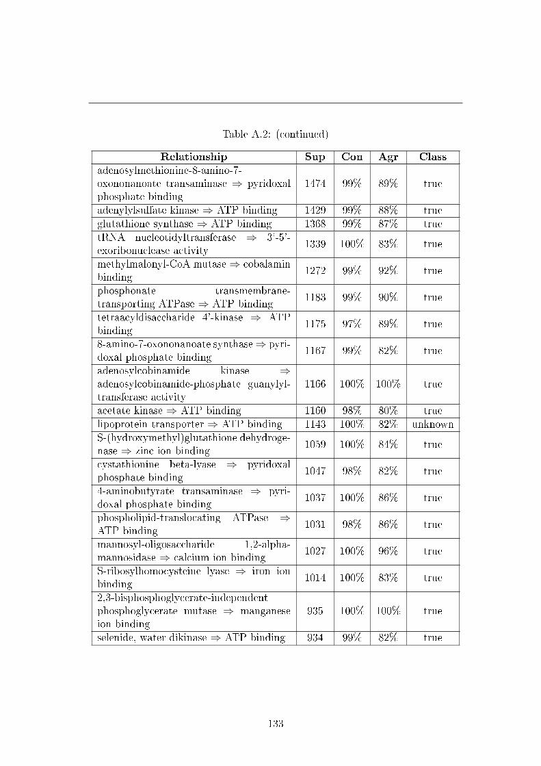
Table A.2: (continued)
Relationship Sup Con Agr Classadenosylmethionine-8-amino-7-oxononanoate transaminase ⇒ pyridoxalphosphate binding
1474 99% 89% true
adenylylsulfate kinase ⇒ ATP binding 1429 99% 88% trueglutathione synthase ⇒ ATP binding 1368 99% 87% truetRNA nucleotidyltransferase ⇒ 3'-5'-exoribonuclease activity
1339 100% 83% true
methylmalonyl-CoA mutase⇒ cobalaminbinding
1272 99% 92% true
phosphonate transmembrane-transporting ATPase ⇒ ATP binding
1183 99% 90% true
tetraacyldisaccharide 4'-kinase ⇒ ATPbinding
1175 97% 89% true
8-amino-7-oxononanoate synthase⇒ pyri-doxal phosphate binding
1167 99% 82% true
adenosylcobinamide kinase ⇒adenosylcobinamide-phosphate guanylyl-transferase activity
1166 100% 100% true
acetate kinase ⇒ ATP binding 1160 98% 80% truelipoprotein transporter ⇒ ATP binding 1143 100% 82% unknownS-(hydroxymethyl)glutathione dehydroge-nase ⇒ zinc ion binding
1059 100% 84% true
cystathionine beta-lyase ⇒ pyridoxalphosphate binding
1047 98% 82% true
4-aminobutyrate transaminase ⇒ pyri-doxal phosphate binding
1037 100% 86% true
phospholipid-translocating ATPase ⇒ATP binding
1031 98% 86% true
mannosyl-oligosaccharide 1,2-alpha-mannosidase ⇒ calcium ion binding
1027 100% 96% true
S-ribosylhomocysteine lyase ⇒ iron ionbinding
1014 100% 83% true
2,3-bisphosphoglycerate-independentphosphoglycerate mutase ⇒ manganeseion binding
935 100% 100% true
selenide, water dikinase ⇒ ATP binding 934 99% 82% true
133

A. MANUAL EVALUATION OF THE GO RELATIONSHIPLEARNING ALGORITHMS
Table A.2: (continued)
Relationship Sup Con Agr Classmagnesium-importing ATPase ⇒ ATPbinding
914 99% 92% true
2-succinyl-5-enolpyruvyl-6-hydroxy-3-cyclohexene-1-carboxylic-acid synthase⇒ thiamin pyrophosphate binding
909 100% 100% true
N2-acetyl-L-ornithine:2-oxoglutarate 5-aminotransferase ⇒ pyridoxal phosphatebinding
890 99% 83% true
DNA clamp loader ⇒ ATP binding 888 100% 100% truecystathionine gamma-synthase ⇒ pyri-doxal phosphate binding
828 99% 87% true
mevalonate kinase ⇒ ATP binding 822 100% 100% truephosphoribulokinase ⇒ ATP binding 800 98% 86% truethymidylate synthase (FAD) ⇒ FADbinding
782 99% 89% true
cytochrome bo3 ubiquinol oxidase⇒ elec-tron carrier activity
777 100% 100% true
O-acetylhomoserine aminocarboxypropyl-transferase ⇒ pyridoxal phosphate bind-ing
745 99% 87% true
xanthine oxidase ⇒ FAD binding 706 99% 92% trueNADPH:quinone reductase ⇒ zinc ionbinding
701 99% 83% true
choline dehydrogenase ⇒ FAD binding 675 99% 88% unknownbiotin carboxylase ⇒ ATP binding 659 97% 86% trueacyl-CoA oxidase ⇒ FAD binding 657 98% 87% trueprotocatechuate 3,4-dioxygenase ⇒ ironion binding
618 99% 86% true
aromatase ⇒ heme binding 617 95% 91% truemicrotubule-severing ATPase ⇒ ATPbinding
612 99% 83% true
dimethyl sulfoxide reductase ⇒ 4 iron, 4sulfur cluster binding
600 100% 100% true
dimethyl sulfoxide reductase ⇒ molybde-num ion binding
600 100% 100% true
aromatase ⇒ electron carrier activity 599 92% 86% true
134
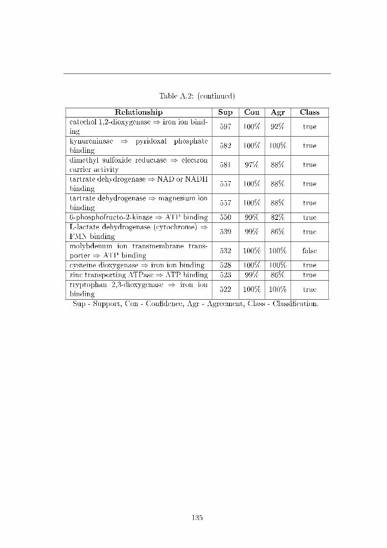
Table A.2: (continued)
Relationship Sup Con Agr Classcatechol 1,2-dioxygenase⇒ iron ion bind-ing
597 100% 92% true
kynureninase ⇒ pyridoxal phosphatebinding
582 100% 100% true
dimethyl sulfoxide reductase ⇒ electroncarrier activity
581 97% 88% true
tartrate dehydrogenase⇒ NAD or NADHbinding
557 100% 88% true
tartrate dehydrogenase⇒ magnesium ionbinding
557 100% 88% true
6-phosphofructo-2-kinase⇒ ATP binding 550 99% 82% trueL-lactate dehydrogenase (cytochrome) ⇒FMN binding
539 99% 86% true
molybdenum ion transmembrane trans-porter ⇒ ATP binding
532 100% 100% false
cysteine dioxygenase ⇒ iron ion binding 528 100% 100% truezinc transporting ATPase⇒ ATP binding 523 99% 86% truetryptophan 2,3-dioxygenase ⇒ iron ionbinding
522 100% 100% true
Sup - Support, Con - Con�dence, Agr - Agreement, Class - Classi�cation.
135

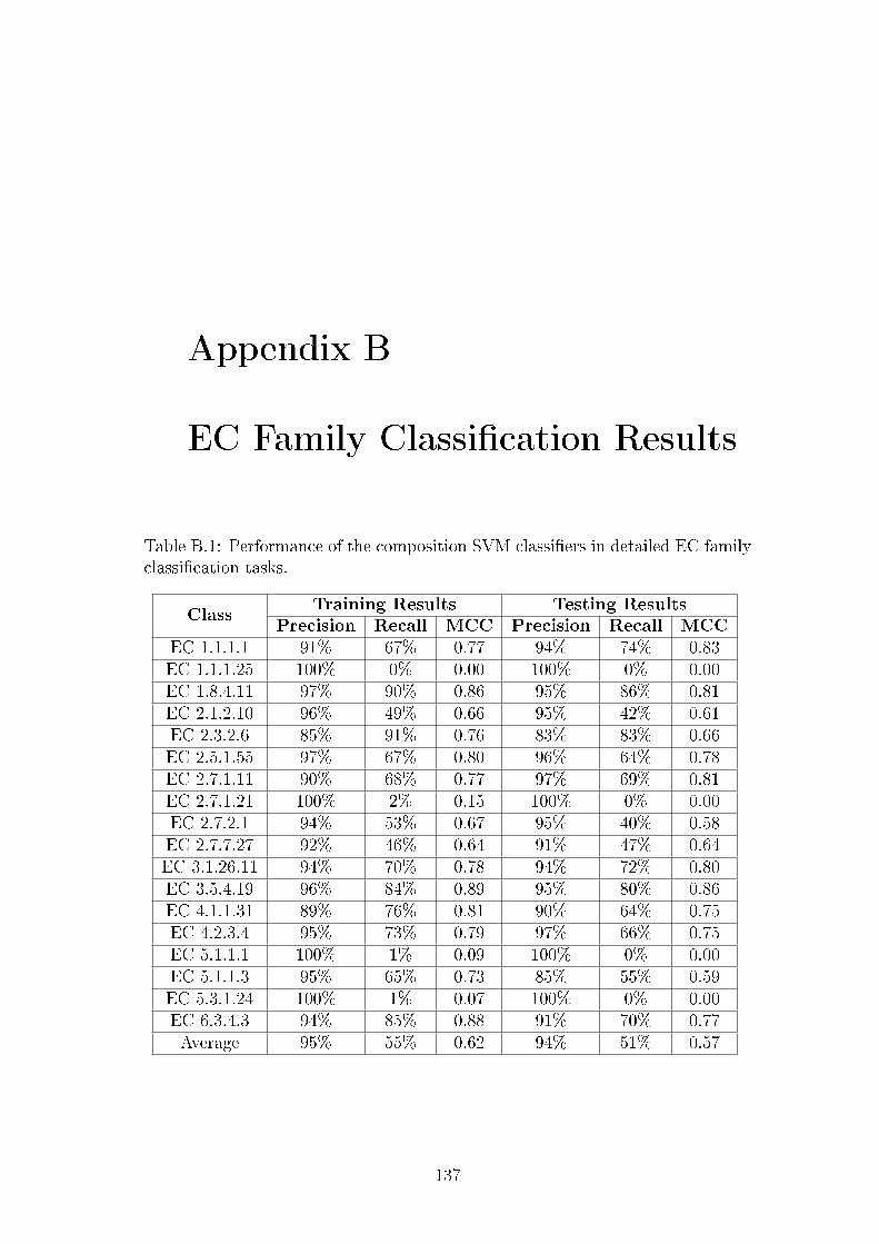
Appendix B
EC Family Classi�cation Results
Table B.1: Performance of the composition SVM classi�ers in detailed EC familyclassi�cation tasks.
ClassTraining Results Testing Results
Precision Recall MCC Precision Recall MCCEC 1.1.1.1 91% 67% 0.77 94% 74% 0.83EC 1.1.1.25 100% 0% 0.00 100% 0% 0.00EC 1.8.4.11 97% 90% 0.86 95% 86% 0.81EC 2.1.2.10 96% 49% 0.66 95% 42% 0.61EC 2.3.2.6 85% 91% 0.76 83% 83% 0.66EC 2.5.1.55 97% 67% 0.80 96% 64% 0.78EC 2.7.1.11 90% 68% 0.77 97% 69% 0.81EC 2.7.1.21 100% 2% 0.15 100% 0% 0.00EC 2.7.2.1 94% 53% 0.67 95% 40% 0.58EC 2.7.7.27 92% 46% 0.64 91% 47% 0.64EC 3.1.26.11 94% 70% 0.78 94% 72% 0.80EC 3.5.4.19 96% 84% 0.89 95% 80% 0.86EC 4.1.1.31 89% 76% 0.81 90% 64% 0.75EC 4.2.3.4 95% 73% 0.79 97% 66% 0.75EC 5.1.1.1 100% 1% 0.09 100% 0% 0.00EC 5.1.1.3 95% 65% 0.73 85% 55% 0.59EC 5.3.1.24 100% 1% 0.07 100% 0% 0.00EC 6.3.4.3 94% 85% 0.88 91% 70% 0.77Average 95% 55% 0.62 94% 51% 0.57
137
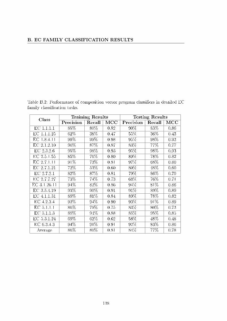
B. EC FAMILY CLASSIFICATION RESULTS
Table B.2: Performance of composition vector program classi�ers in detailed ECfamily classi�cation tasks.
ClassTraining Results Testing Results
Precision Recall MCC Precision Recall MCCEC 1.1.1.1 85% 80% 0.82 90% 83% 0.86EC 1.1.1.25 62% 38% 0.47 55% 36% 0.43EC 1.8.4.11 99% 99% 0.98 95% 98% 0.93EC 2.1.2.10 90% 87% 0.87 83% 77% 0.77EC 2.3.2.6 95% 98% 0.93 95% 98% 0.93EC 2.5.1.55 85% 76% 0.80 89% 78% 0.82EC 2.7.1.11 91% 73% 0.81 97% 68% 0.80EC 2.7.1.21 72% 53% 0.60 80% 48% 0.60EC 2.7.2.1 82% 87% 0.81 79% 86% 0.79EC 2.7.7.27 73% 74% 0.73 68% 76% 0.71EC 3.1.26.11 94% 82% 0.86 94% 81% 0.86EC 3.5.4.19 93% 90% 0.91 91% 89% 0.89EC 4.1.1.31 89% 81% 0.84 89% 78% 0.82EC 4.2.3.4 92% 94% 0.90 93% 91% 0.89EC 5.1.1.1 86% 79% 0.75 83% 80% 0.73EC 5.1.1.3 89% 94% 0.88 85% 95% 0.85EC 5.3.1.24 69% 62% 0.62 58% 48% 0.48EC 6.3.4.3 94% 91% 0.91 92% 83% 0.86Average 86% 80% 0.81 84% 77% 0.78
138
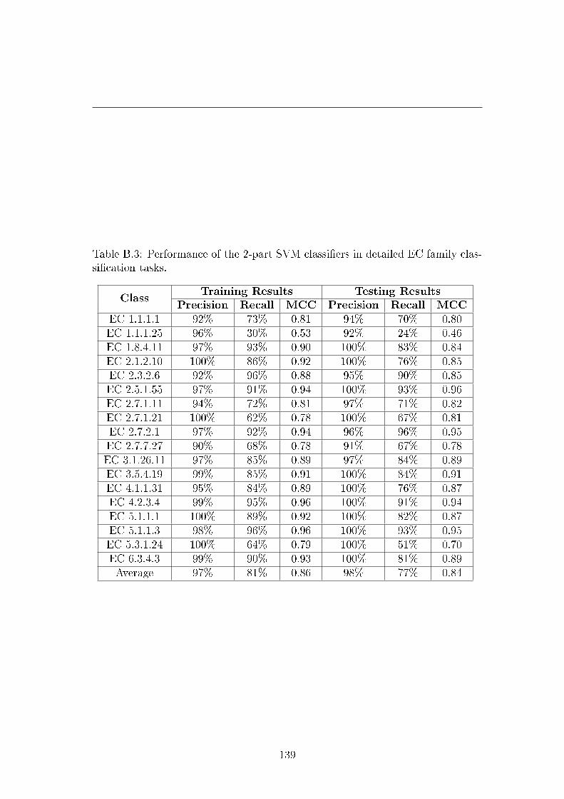
Table B.3: Performance of the 2-part SVM classi�ers in detailed EC family clas-si�cation tasks.
ClassTraining Results Testing Results
Precision Recall MCC Precision Recall MCCEC 1.1.1.1 92% 73% 0.81 94% 70% 0.80EC 1.1.1.25 96% 30% 0.53 92% 24% 0.46EC 1.8.4.11 97% 93% 0.90 100% 83% 0.84EC 2.1.2.10 100% 86% 0.92 100% 76% 0.85EC 2.3.2.6 92% 96% 0.88 95% 90% 0.85EC 2.5.1.55 97% 91% 0.94 100% 93% 0.96EC 2.7.1.11 94% 72% 0.81 97% 71% 0.82EC 2.7.1.21 100% 62% 0.78 100% 67% 0.81EC 2.7.2.1 97% 92% 0.94 96% 96% 0.95EC 2.7.7.27 90% 68% 0.78 91% 67% 0.78EC 3.1.26.11 97% 85% 0.89 97% 84% 0.89EC 3.5.4.19 99% 85% 0.91 100% 84% 0.91EC 4.1.1.31 95% 84% 0.89 100% 76% 0.87EC 4.2.3.4 99% 95% 0.96 100% 91% 0.94EC 5.1.1.1 100% 89% 0.92 100% 82% 0.87EC 5.1.1.3 98% 96% 0.96 100% 93% 0.95EC 5.3.1.24 100% 64% 0.79 100% 51% 0.70EC 6.3.4.3 99% 90% 0.93 100% 81% 0.89Average 97% 81% 0.86 98% 77% 0.84
139
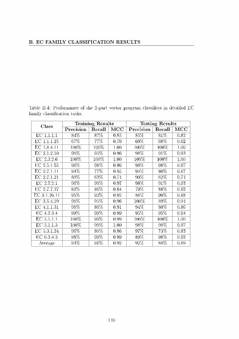
B. EC FAMILY CLASSIFICATION RESULTS
Table B.4: Performance of the 2-part vector program classi�ers in detailed ECfamily classi�cation tasks.
ClassTraining Results Testing Results
Precision Recall MCC Precision Recall MCCEC 1.1.1.1 84% 87% 0.85 85% 81% 0.82EC 1.1.1.25 67% 77% 0.70 60% 68% 0.62EC 1.8.4.11 100% 100% 1.00 100% 100% 1.00EC 2.1.2.10 98% 95% 0.96 98% 91% 0.93EC 2.3.2.6 100% 100% 1.00 100% 100% 1.00EC 2.5.1.55 96% 98% 0.96 98% 98% 0.97EC 2.7.1.11 94% 77% 0.85 94% 80% 0.87EC 2.7.1.21 89% 63% 0.74 90% 62% 0.74EC 2.7.2.1 96% 99% 0.97 98% 91% 0.93EC 2.7.7.27 82% 86% 0.84 79% 88% 0.83EC 3.1.26.11 95% 92% 0.92 88% 90% 0.88EC 3.5.4.19 98% 95% 0.96 100% 89% 0.94EC 4.1.1.31 98% 86% 0.91 94% 80% 0.86EC 4.2.3.4 99% 99% 0.99 95% 95% 0.94EC 5.1.1.1 100% 99% 0.99 100% 100% 1.00EC 5.1.1.3 100% 99% 1.00 98% 98% 0.97EC 5.3.1.24 96% 80% 0.86 97% 73% 0.83EC 6.3.4.3 98% 99% 0.99 89% 98% 0.92Average 94% 91% 0.92 92% 88% 0.89
140

Table B.5: Performance of the 4-part SVM classi�ers in detailed EC family clas-si�cation tasks.
ClassTraining Results Testing Results
Precision Recall MCC Precision Recall MCCEC 1.1.1.1 96% 94% 0.95 86% 88% 0.87EC 1.1.1.25 100% 97% 0.98 100% 89% 0.94EC 1.8.4.11 100% 100% 1.00 100% 98% 0.98EC 2.1.2.10 100% 100% 1.00 100% 98% 0.99EC 2.3.2.6 100% 99% 0.99 100% 95% 0.95EC 2.5.1.55 100% 100% 1.00 100% 98% 0.99EC 2.7.1.11 99% 94% 0.96 91% 93% 0.91EC 2.7.1.21 100% 98% 0.99 93% 88% 0.90EC 2.7.2.1 99% 100% 1.00 100% 98% 0.99EC 2.7.7.27 100% 100% 1.00 100% 95% 0.98EC 3.1.26.11 100% 95% 0.97 98% 93% 0.95EC 3.5.4.19 100% 98% 0.99 100% 93% 0.96EC 4.1.1.31 100% 98% 0.99 95% 93% 0.94EC 4.2.3.4 100% 98% 0.98 100% 91% 0.94EC 5.1.1.1 100% 100% 1.00 100% 98% 0.98EC 5.1.1.3 100% 99% 1.00 100% 99% 1.00EC 5.3.1.24 99% 94% 0.96 100% 87% 0.92EC 6.3.4.3 100% 99% 0.99 100% 93% 0.96Average 100% 98% 0.99 98% 94% 0.95
141
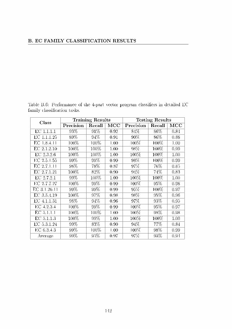
B. EC FAMILY CLASSIFICATION RESULTS
Table B.6: Performance of the 4-part vector program classi�ers in detailed ECfamily classi�cation tasks.
ClassTraining Results Testing Results
Precision Recall MCC Precision Recall MCCEC 1.1.1.1 93% 91% 0.92 84% 86% 0.84EC 1.1.1.25 89% 94% 0.91 90% 86% 0.88EC 1.8.4.11 100% 100% 1.00 100% 100% 1.00EC 2.1.2.10 100% 100% 1.00 98% 100% 0.99EC 2.3.2.6 100% 100% 1.00 100% 100% 1.00EC 2.5.1.55 99% 99% 0.99 98% 100% 0.99EC 2.7.1.11 98% 78% 0.87 97% 76% 0.85EC 2.7.1.21 100% 82% 0.90 94% 74% 0.83EC 2.7.2.1 99% 100% 1.00 100% 100% 1.00EC 2.7.7.27 100% 99% 0.99 100% 95% 0.98EC 3.1.26.11 99% 99% 0.99 95% 100% 0.97EC 3.5.4.19 100% 97% 0.98 98% 95% 0.96EC 4.1.1.31 98% 94% 0.96 97% 93% 0.95EC 4.2.3.4 100% 99% 0.99 100% 95% 0.97EC 5.1.1.1 100% 100% 1.00 100% 98% 0.98EC 5.1.1.3 100% 99% 1.00 100% 100% 1.00EC 5.3.1.24 99% 83% 0.90 94% 77% 0.84EC 6.3.4.3 99% 100% 1.00 100% 98% 0.99Average 99% 95% 0.97 97% 93% 0.94
142

Table B.7: Performance of the 6-part SVM classi�ers in detailed EC family clas-si�cation tasks.
ClassTraining Results Testing Results
Precision Recall MCC Precision Recall MCCEC 1.1.1.1 100% 100% 1.00 95% 88% 0.91EC 1.1.1.25 100% 99% 0.99 100% 93% 0.96EC 1.8.4.11 100% 100% 1.00 100% 98% 0.98EC 2.1.2.10 100% 100% 1.00 100% 98% 0.99EC 2.3.2.6 100% 100% 1.00 100% 98% 0.98EC 2.5.1.55 100% 100% 1.00 100% 98% 0.99EC 2.7.1.11 100% 100% 1.00 95% 95% 0.95EC 2.7.1.21 100% 100% 1.00 100% 91% 0.95EC 2.7.2.1 100% 100% 1.00 100% 98% 0.99EC 2.7.7.27 100% 100% 1.00 100% 98% 0.99EC 3.1.26.11 100% 100% 1.00 98% 95% 0.96EC 3.5.4.19 100% 100% 1.00 98% 96% 0.96EC 4.1.1.31 100% 100% 1.00 98% 98% 0.97EC 4.2.3.4 100% 99% 1.00 100% 93% 0.95EC 5.1.1.1 100% 100% 1.00 100% 98% 0.98EC 5.1.1.3 100% 99% 1.00 100% 98% 0.98EC 5.3.1.24 100% 99% 0.99 98% 98% 0.98EC 6.3.4.3 100% 100% 1.00 95% 98% 0.96Average 100% 100% 1.00 99% 96% 0.97
143

B. EC FAMILY CLASSIFICATION RESULTS
Table B.8: Performance of the 6-part vector program classi�ers in detailed ECfamily classi�cation tasks.
ClassTraining Results Testing Results
Precision Recall MCC Precision Recall MCCEC 1.1.1.1 97% 91% 0.94 90% 88% 0.89EC 1.1.1.25 99% 96% 0.98 98% 95% 0.96EC 1.8.4.11 100% 100% 1.00 100% 100% 1.00EC 2.1.2.10 100% 100% 1.00 100% 100% 1.00EC 2.3.2.6 100% 100% 1.00 100% 100% 1.00EC 2.5.1.55 100% 100% 1.00 100% 100% 1.00EC 2.7.1.11 99% 90% 0.94 100% 90% 0.95EC 2.7.1.21 100% 88% 0.93 90% 86% 0.87EC 2.7.2.1 100% 100% 1.00 100% 100% 1.00EC 2.7.7.27 99% 99% 0.99 98% 100% 0.99EC 3.1.26.11 100% 99% 1.00 95% 98% 0.96EC 3.5.4.19 100% 100% 1.00 98% 93% 0.95EC 4.1.1.31 100% 98% 0.99 95% 95% 0.95EC 4.2.3.4 100% 100% 1.00 100% 98% 0.98EC 5.1.1.1 100% 100% 1.00 100% 100% 1.00EC 5.1.1.3 100% 100% 1.00 100% 100% 1.00EC 5.3.1.24 99% 89% 0.93 95% 86% 0.90EC 6.3.4.3 100% 100% 1.00 98% 100% 0.99Average 100% 97% 0.98 98% 96% 0.97
144
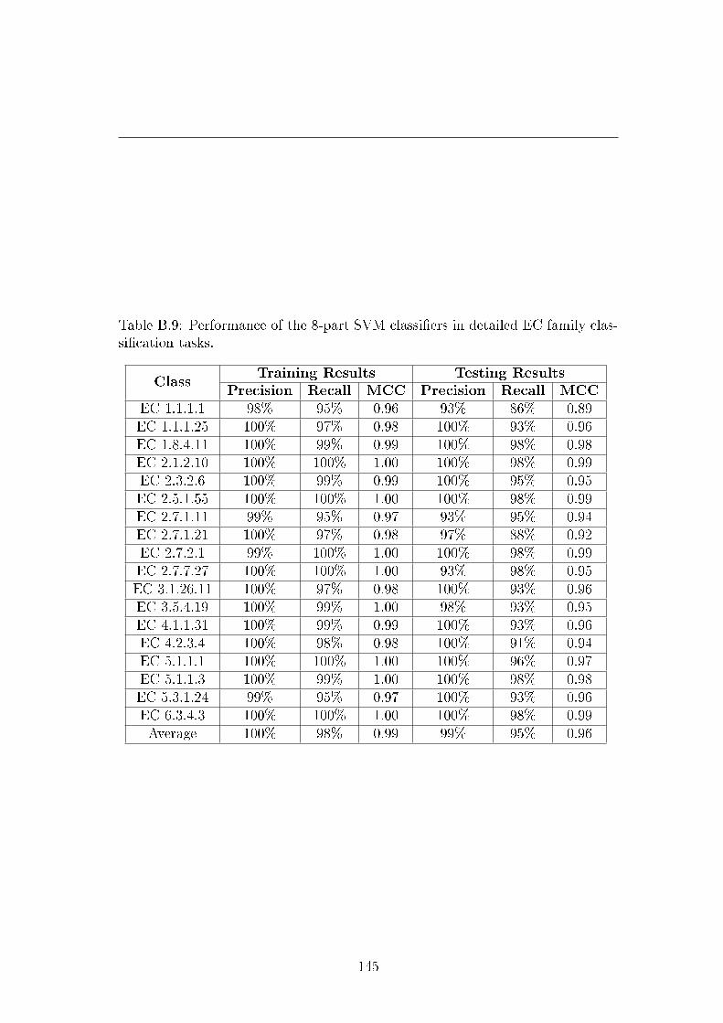
Table B.9: Performance of the 8-part SVM classi�ers in detailed EC family clas-si�cation tasks.
ClassTraining Results Testing Results
Precision Recall MCC Precision Recall MCCEC 1.1.1.1 98% 95% 0.96 93% 86% 0.89EC 1.1.1.25 100% 97% 0.98 100% 93% 0.96EC 1.8.4.11 100% 99% 0.99 100% 98% 0.98EC 2.1.2.10 100% 100% 1.00 100% 98% 0.99EC 2.3.2.6 100% 99% 0.99 100% 95% 0.95EC 2.5.1.55 100% 100% 1.00 100% 98% 0.99EC 2.7.1.11 99% 95% 0.97 93% 95% 0.94EC 2.7.1.21 100% 97% 0.98 97% 88% 0.92EC 2.7.2.1 99% 100% 1.00 100% 98% 0.99EC 2.7.7.27 100% 100% 1.00 93% 98% 0.95EC 3.1.26.11 100% 97% 0.98 100% 93% 0.96EC 3.5.4.19 100% 99% 1.00 98% 93% 0.95EC 4.1.1.31 100% 99% 0.99 100% 93% 0.96EC 4.2.3.4 100% 98% 0.98 100% 91% 0.94EC 5.1.1.1 100% 100% 1.00 100% 96% 0.97EC 5.1.1.3 100% 99% 1.00 100% 98% 0.98EC 5.3.1.24 99% 95% 0.97 100% 93% 0.96EC 6.3.4.3 100% 100% 1.00 100% 98% 0.99Average 100% 98% 0.99 99% 95% 0.96
145

B. EC FAMILY CLASSIFICATION RESULTS
Table B.10: Performance of the 8-part vector program classi�ers in detailed ECfamily classi�cation tasks.
ClassTraining Results Testing Results
Precision Recall MCC Precision Recall MCCEC 1.1.1.1 98% 94% 0.96 90% 83% 0.86EC 1.1.1.25 100% 96% 0.98 95% 93% 0.94EC 1.8.4.11 100% 100% 1.00 100% 98% 0.98EC 2.1.2.10 100% 100% 1.00 100% 100% 1.00EC 2.3.2.6 100% 100% 1.00 100% 100% 1.00EC 2.5.1.55 100% 100% 1.00 95% 100% 0.97EC 2.7.1.11 99% 81% 0.89 100% 78% 0.88EC 2.7.1.21 100% 93% 0.96 92% 79% 0.84EC 2.7.2.1 100% 100% 1.00 98% 100% 0.99EC 2.7.7.27 100% 100% 1.00 95% 98% 0.96EC 3.1.26.11 100% 100% 1.00 95% 90% 0.92EC 3.5.4.19 100% 98% 0.99 95% 89% 0.91EC 4.1.1.31 100% 94% 0.97 97% 88% 0.92EC 4.2.3.4 100% 100% 1.00 100% 95% 0.97EC 5.1.1.1 100% 100% 1.00 100% 100% 1.00EC 5.1.1.3 100% 100% 1.00 100% 100% 1.00EC 5.3.1.24 100% 83% 0.90 94% 77% 0.84EC 6.3.4.3 100% 100% 1.00 98% 100% 0.99Average 100% 97% 0.98 97% 93% 0.94
146

Table B.11: Performance of two nearest-neighbors classi�ers based on the TripSimmeasure in detailed EC family classi�cation tasks.
Classsingle-neighbor 10% neighborhood
Precision Recall MCC Precision Recall MCCEC 1.1.1.1 95% 98% 0.96 95% 93% 0.94EC 1.1.1.25 100% 98% 0.99 98% 93% 0.95EC 1.8.4.11 100% 98% 0.98 100% 98% 0.98EC 2.1.2.10 100% 100% 1.00 100% 100% 1.00EC 2.3.2.6 100% 98% 0.98 100% 98% 0.98EC 2.5.1.55 100% 100% 1.00 100% 100% 1.00EC 2.7.1.11 100% 98% 0.99 98% 95% 0.96EC 2.7.1.21 100% 88% 0.94 100% 88% 0.94EC 2.7.2.1 100% 100% 1.00 98% 100% 0.99EC 2.7.7.27 100% 100% 1.00 100% 100% 1.00EC 3.1.26.11 100% 100% 1.00 100% 98% 0.99EC 3.5.4.19 100% 100% 1.00 100% 100% 1.00EC 4.1.1.31 98% 100% 0.99 93% 98% 0.95EC 4.2.3.4 100% 100% 1.00 98% 100% 0.98EC 5.1.1.1 100% 91% 0.93 100% 91% 0.93EC 5.1.1.3 98% 100% 0.98 98% 100% 0.98EC 5.3.1.24 100% 98% 0.99 91% 98% 0.94EC 6.3.4.3 100% 100% 1.00 98% 100% 0.99Average 99% 98% 0.98 98% 97% 0.97
147


Appendix C
Underrepresented and
Overrepresented Dipeptides and
Tripeptides in UniProtKB
149
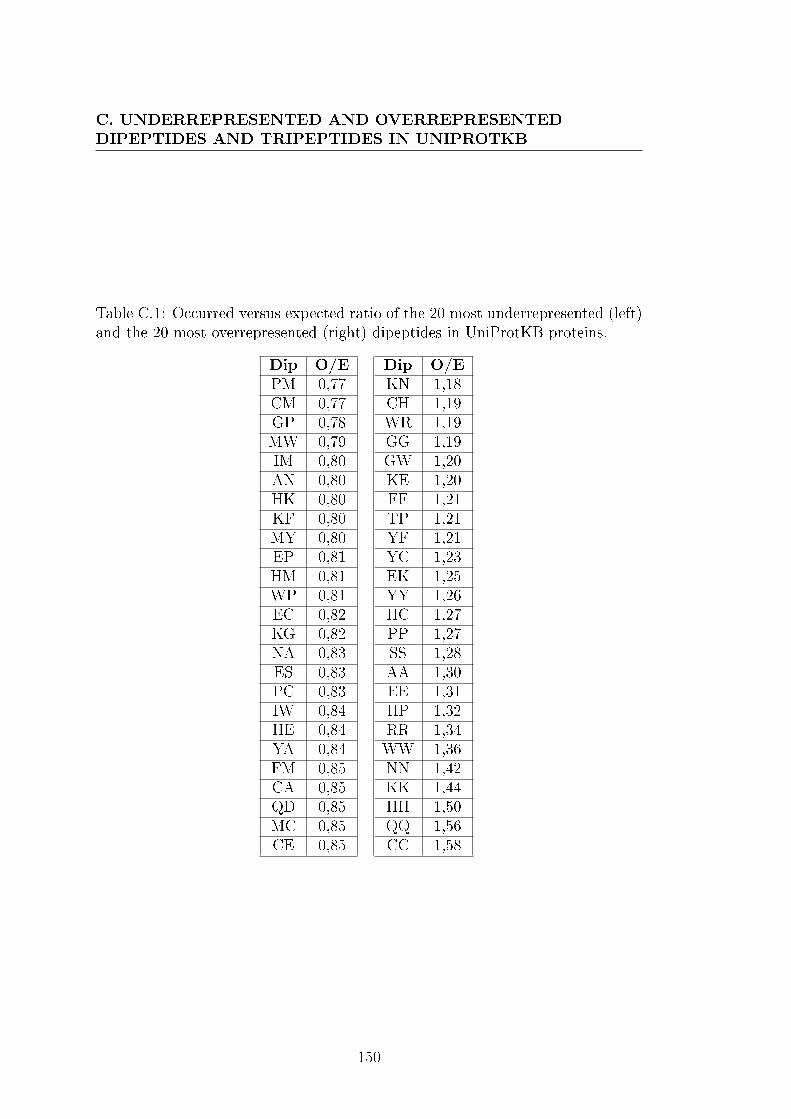
C. UNDERREPRESENTED AND OVERREPRESENTEDDIPEPTIDES AND TRIPEPTIDES IN UNIPROTKB
Table C.1: Occurred versus expected ratio of the 20 most underrepresented (left)and the 20 most overrepresented (right) dipeptides in UniProtKB proteins.
Dip O/E Dip O/EPM 0,77 KN 1,18CM 0,77 CH 1,19GP 0,78 WR 1,19MW 0,79 GG 1,19IM 0,80 GW 1,20AN 0,80 KE 1,20HK 0,80 FF 1,21KF 0,80 TP 1,21MY 0,80 YF 1,21EP 0,81 YC 1,23HM 0,81 EK 1,25WP 0,81 YY 1,26EC 0,82 HC 1,27KG 0,82 PP 1,27NA 0,83 SS 1,28ES 0,83 AA 1,30PC 0,83 EE 1,31IW 0,84 HP 1,32HE 0,84 RR 1,34YA 0,84 WW 1,36FM 0,85 NN 1,42CA 0,85 KK 1,44QD 0,85 HH 1,50MC 0,85 QQ 1,56CE 0,85 CC 1,58
150

Table C.2: Occurred versus expected ratio of the 20 most underrepresented (left)and the 20 most overrepresented (right) tripeptides in UniProtKB proteins.
Trip O/E Trip O/EKCA 0,48 WIW 2,28KGP 0,51 CSC 2,29PCM 0,53 HHP 2,30KWP 0,53 MHY 2,32IMW 0,55 NCT 2,33MWP 0,55 FYC 2,36PMK 0,56 RRR 2,39EGP 0,56 CVC 2,40EWP 0,57 CGH 2,41MWV 0,58 SSS 2,44EPN 0,58 YCN 2,46WPK 0,60 YWW 2,47AKC 0,60 HHM 2,53LMY 0,60 WQR 2,54WPM 0,60 HYC 2,82FKW 0,60 KKK 2,93KMW 0,60 YQY 2,96EMW 0,60 WYW 3,10KFA 0,61 HCN 3,19PME 0,61 PPP 3,39FKM 0,61 WWN 3,80WEF 0,61 NNN 4,49WPY 0,61 HHH 5,23ECA 0,62 QQQ 5,90KFM 0,62 CCC 6,64
151


Appendix D
Molecular Function Annotation
Prediction Results
Table D.1: Molecular function annotation prediction results with twoBLAST classi�ers.
ProteinSingle Neighbor 10% Neighborhood
Hits simGIC Precision Hits simGIC PrecisionA3KPF2 1 7% 100% 1 7% 100%O00764 2 34% 100% 6 40% 100%O05783 3 40% 100% 3 40% 100%O05891 17 54% 100% 18 54% 100%O35217 1 100% 100% 6 100% 100%O49203 1 70% 100% 6 70% 100%O49543 1 57% 100% 1 57% 100%O53434 5 13% 33% 23 13% 33%O60674 1 71% 100% 9 71% 100%O60760 1 71% 100% 2 71% 100%O70503 1 61% 100% 2 61% 100%O75908 1 24% 100% 2 24% 100%O80803 1 47% 100% 4 47% 100%P00367 1 48% 100% 12 47% 100%P00509 42 30% 100% 143 30% 100%P00957 6 57% 100% 120 57% 100%P04041 2 24% 59% 3 24% 59%P04693 9 29% 100% 106 29% 100%
153
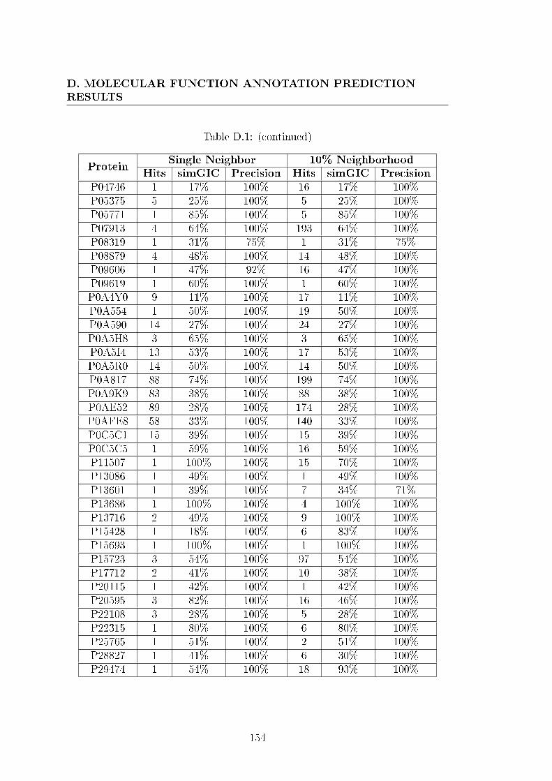
D. MOLECULAR FUNCTION ANNOTATION PREDICTIONRESULTS
Table D.1: (continued)
ProteinSingle Neighbor 10% Neighborhood
Hits simGIC Precision Hits simGIC PrecisionP04746 1 17% 100% 16 17% 100%P05375 5 25% 100% 5 25% 100%P05771 1 85% 100% 5 85% 100%P07913 4 64% 100% 193 64% 100%P08319 1 31% 75% 1 31% 75%P08879 4 48% 100% 14 48% 100%P09606 1 47% 92% 16 47% 100%P09619 1 60% 100% 1 60% 100%P0A4Y0 9 11% 100% 17 11% 100%P0A554 1 50% 100% 19 50% 100%P0A590 14 27% 100% 24 27% 100%P0A5H8 3 65% 100% 3 65% 100%P0A5I4 13 53% 100% 17 53% 100%P0A5R0 14 50% 100% 14 50% 100%P0A817 88 74% 100% 199 74% 100%P0A9K9 83 38% 100% 88 38% 100%P0AE52 89 28% 100% 174 28% 100%P0AFE8 58 33% 100% 140 33% 100%P0C5C1 15 39% 100% 15 39% 100%P0C5C5 1 59% 100% 16 59% 100%P11507 1 100% 100% 15 70% 100%P13086 1 49% 100% 1 49% 100%P13601 1 39% 100% 7 34% 71%P13686 1 100% 100% 4 100% 100%P13716 2 49% 100% 9 100% 100%P15428 1 18% 100% 6 83% 100%P15693 1 100% 100% 1 100% 100%P15723 3 54% 100% 97 54% 100%P17712 2 41% 100% 10 38% 100%P20115 1 42% 100% 1 42% 100%P20595 3 82% 100% 16 46% 100%P22108 3 28% 100% 5 28% 100%P22315 1 80% 100% 6 80% 100%P25765 1 51% 100% 2 51% 100%P28827 1 41% 100% 6 30% 100%P29474 1 54% 100% 18 93% 100%
154

Table D.1: (continued)
ProteinSingle Neighbor 10% Neighborhood
Hits simGIC Precision Hits simGIC PrecisionP30416 1 86% 86% 6 100% 100%P32662 19 42% 100% 128 42% 100%P32961 1 8% 100% 2 8% 100%P32962 1 8% 100% 6 8% 100%P34760 3 8% 100% 14 8% 100%P35520 1 42% 100% 3 42% 100%P35610 2 9% 100% 7 31% 100%P36970 1 48% 100% 12 48% 100%P38274 1 9% 100% 4 9% 100%P39518 1 38% 100% 7 38% 100%P40394 1 50% 77% 7 50% 77%P41682 1 100% 100% 7 100% 100%P42760 1 100% 100% 1 100% 100%P46010 1 8% 100% 2 8% 100%P46011 1 7% 100% 2 7% 100%P46248 1 54% 100% 3 54% 100%P47712 1 52% 100% 13 38% 100%P49186 1 49% 100% 10 35% 100%P49448 1 100% 100% 8 61% 100%P49615 4 26% 100% 14 26% 100%P50521 1 57% 100% 1 57% 100%P51433 1 100% 100% 3 48% 100%P51647 1 100% 100% 7 47% 100%P60479 17 33% 100% 17 33% 100%P61086 7 53% 100% 14 27% 100%P64012 13 33% 87% 17 33% 87%P66930 17 65% 100% 22 65% 100%P70352 1 100% 100% 3 100% 100%P75820 6 40% 100% 95 40% 100%P77489 1 49% 100% 2 49% 100%P78536 1 30% 100% 19 30% 100%P83483 2 83% 100% 6 83% 100%P83734 17 5% 100% 19 5% 100%P93834 1 70% 100% 1 70% 100%P96420 8 26% 100% 11 26% 100%P96864 14 20% 100% 16 20% 100%
155

D. MOLECULAR FUNCTION ANNOTATION PREDICTIONRESULTS
Table D.1: (continued)
ProteinSingle Neighbor 10% Neighborhood
Hits simGIC Precision Hits simGIC PrecisionP97523 1 100% 100% 5 58% 100%Q01292 1 41% 100% 24 41% 100%Q01814 2 100% 100% 7 67% 91%Q02759 2 69% 100% 2 69% 100%Q02972 1 17% 100% 1 17% 100%Q04894 4 13% 100% 5 13% 100%Q07014 2 100% 100% 11 29% 100%Q08220 3 35% 100% 6 35% 100%Q08257 1 36% 100% 2 36% 100%Q09756 1 57% 100% 1 57% 100%Q13526 1 23% 100% 6 100% 100%Q14694 1 100% 100% 5 100% 100%Q16512 1 100% 100% 5 91% 100%Q21815 1 33% 100% 1 33% 100%Q2LAE1 1 74% 100% 1 74% 100%Q38946 1 20% 100% 5 20% 100%Q43314 1 23% 100% 16 23% 100%Q56XE8 1 47% 100% 1 47% 100%Q5EAF2 1 17% 62% 1 17% 62%Q60587 1 100% 100% 6 21% 100%Q62658 5 59% 100% 21 19% 100%Q62689 1 100% 100% 12 57% 100%Q62925 1 34% 100% 8 34% 100%Q64428 1 100% 100% 5 42% 100%Q66HA1 1 100% 100% 2 100% 100%Q6PFW1 1 17% 100% 9 17% 100%Q7D785 1 48% 100% 1 48% 100%Q84W92 1 7% 100% 1 7% 100%Q8BU27 1 36% 100% 1 36% 100%Q8GZB6 1 45% 100% 1 45% 100%Q8H1Y0 1 60% 100% 1 60% 100%Q8VZC3 2 3% 8% 2 3% 8%Q91XR8 1 100% 100% 1 100% 100%Q945K7 1 71% 100% 2 71% 100%Q99683 1 23% 100% 5 25% 100%Q9C5I1 1 8% 100% 1 8% 100%
156

Table D.1: (continued)
ProteinSingle Neighbor 10% Neighborhood
Hits simGIC Precision Hits simGIC PrecisionQ9C8G9 1 31% 100% 1 31% 100%Q9FK25 1 35% 100% 2 35% 100%Q9FKL8 1 100% 100% 3 47% 100%Q9FKL9 1 47% 100% 2 47% 100%Q9FN42 1 41% 100% 1 41% 100%Q9FZG4 1 70% 100% 1 70% 100%Q9GZT4 1 78% 100% 2 78% 100%Q9JHW9 1 100% 100% 6 88% 100%Q9JI61 2 100% 100% 2 100% 100%Q9LDD8 1 6% 100% 1 6% 100%Q9LK64 1 47% 100% 2 47% 100%Q9LPS1 1 47% 100% 1 47% 100%Q9M0D1 1 47% 100% 8 47% 100%Q9M0D2 1 47% 100% 8 47% 100%Q9NQW7 1 45% 100% 9 100% 100%Q9NST1 1 100% 100% 1 100% 100%Q9QYY9 1 100% 100% 4 100% 100%Q9QZX7 2 78% 100% 8 78% 100%Q9SRY5 1 100% 100% 1 100% 100%Q9T071 1 47% 100% 1 47% 100%Q9WUD9 1 94% 94% 17 40% 100%Q9Z286 1 42% 100% 3 79% 100%Average 5 52% 98% 16 49% 98%
Table D.2: Molecular function annotation prediction results with two Trip-Sim classi�ers.
ProteinSingle Neighbor 10% Neighborhood
Hits simGIC Precision Hits simGIC PrecisionA3KPF2 1 7% 100% 1 7% 100%O00764 1 34% 100% 5 40% 100%O05783 3 40% 100% 3 40% 100%O05891 17 54% 100% 18 54% 100%O35217 1 100% 100% 2 100% 100%O49203 1 70% 100% 2 70% 100%O49543 1 57% 100% 2 57% 100%
157
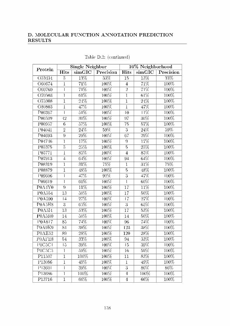
D. MOLECULAR FUNCTION ANNOTATION PREDICTIONRESULTS
Table D.2: (continued)
ProteinSingle Neighbor 10% Neighborhood
Hits simGIC Precision Hits simGIC PrecisionO53434 5 13% 33% 15 13% 33%O60674 1 71% 100% 4 71% 100%O60760 1 71% 100% 2 71% 100%O70503 1 61% 100% 1 61% 100%O75908 1 24% 100% 1 24% 100%O80803 1 47% 100% 1 47% 100%P00367 1 51% 100% 10 11% 100%P00509 42 30% 100% 97 30% 100%P00957 6 57% 100% 75 57% 100%P04041 2 24% 59% 3 24% 59%P04693 9 29% 100% 67 29% 100%P04746 1 17% 100% 9 17% 100%P05375 5 25% 100% 5 25% 100%P05771 1 85% 100% 4 85% 100%P07913 4 64% 100% 94 64% 100%P08319 1 31% 75% 1 31% 75%P08879 1 48% 100% 5 48% 100%P09606 1 47% 92% 3 47% 100%P09619 1 60% 100% 1 60% 100%P0A4Y0 9 11% 100% 17 11% 100%P0A554 13 50% 100% 17 50% 100%P0A590 14 27% 100% 17 27% 100%P0A5H8 3 65% 100% 3 65% 100%P0A5I4 13 53% 100% 17 53% 100%P0A5R0 14 50% 100% 14 50% 100%P0A817 85 74% 100% 96 74% 100%P0A9K9 84 38% 100% 123 38% 100%P0AE52 89 28% 100% 120 28% 100%P0AFE8 54 33% 100% 94 33% 100%P0C5C1 15 39% 100% 15 39% 100%P0C5C5 1 59% 100% 16 59% 100%P11507 1 100% 100% 11 83% 100%P13086 1 49% 100% 1 49% 100%P13601 1 39% 100% 3 86% 86%P13686 1 100% 100% 4 100% 100%P13716 1 66% 100% 4 66% 100%
158

Table D.2: (continued)
ProteinSingle Neighbor 10% Neighborhood
Hits simGIC Precision Hits simGIC PrecisionP15428 1 18% 100% 2 18% 100%P15693 1 100% 100% 1 100% 100%P15723 3 54% 100% 91 54% 100%P17712 2 41% 100% 8 41% 100%P20115 1 42% 100% 1 42% 100%P20595 1 82% 100% 13 46% 100%P22108 2 28% 100% 5 28% 100%P22315 1 80% 100% 3 80% 100%P25765 1 51% 100% 2 51% 100%P28827 1 41% 100% 3 30% 100%P29474 1 54% 100% 1 54% 100%P30416 1 86% 86% 1 86% 86%P32662 18 42% 100% 90 42% 100%P32961 1 8% 100% 2 8% 100%P32962 1 8% 100% 2 8% 100%P34760 3 8% 100% 4 8% 100%P35520 1 42% 100% 2 42% 100%P35610 1 77% 100% 8 31% 100%P36970 1 48% 100% 4 29% 100%P38274 1 9% 100% 4 9% 100%P39518 1 5% 100% 9 38% 100%P40394 1 6% 100% 2 6% 100%P41682 2 100% 100% 4 100% 100%P42760 1 100% 100% 1 100% 100%P46010 1 8% 100% 1 8% 100%P46011 1 7% 100% 1 7% 100%P46248 1 54% 100% 3 54% 100%P47712 1 52% 100% 3 38% 100%P49186 1 49% 100% 8 35% 100%P49448 1 100% 100% 3 100% 100%P49615 4 26% 100% 9 50% 100%P50521 1 57% 100% 1 57% 100%P51433 1 48% 100% 2 48% 100%P51647 1 100% 100% 1 100% 100%P60479 17 33% 100% 17 33% 100%P61086 7 53% 100% 8 53% 100%
159

D. MOLECULAR FUNCTION ANNOTATION PREDICTIONRESULTS
Table D.2: (continued)
ProteinSingle Neighbor 10% Neighborhood
Hits simGIC Precision Hits simGIC PrecisionP64012 13 33% 87% 17 33% 87%P66930 17 65% 100% 17 65% 100%P70352 1 100% 100% 2 100% 100%P75820 6 40% 100% 86 40% 100%P77489 1 40% 100% 2 40% 100%P78536 1 30% 100% 1 30% 100%P83483 2 83% 100% 4 83% 100%P83734 17 5% 100% 17 5% 100%P93834 1 70% 100% 2 70% 100%P96420 7 26% 100% 15 26% 100%P96864 14 20% 100% 16 20% 100%P97523 1 100% 100% 1 100% 100%Q01292 1 34% 100% 25 41% 100%Q01814 1 72% 100% 8 72% 100%Q02759 2 69% 100% 2 69% 100%Q02972 1 17% 100% 1 17% 100%Q04894 4 13% 100% 5 13% 100%Q07014 2 100% 100% 7 43% 100%Q08220 3 35% 100% 6 35% 100%Q08257 1 36% 100% 1 36% 100%Q09756 1 57% 100% 92 57% 100%Q13526 1 23% 100% 3 23% 100%Q14694 1 100% 100% 4 100% 100%Q16512 1 100% 100% 3 100% 100%Q21815 1 33% 100% 1 33% 100%Q2LAE1 1 74% 100% 1 74% 100%Q38946 1 20% 100% 1 20% 100%Q43314 1 23% 100% 2 23% 100%Q56XE8 1 47% 100% 1 47% 100%Q5EAF2 1 17% 62% 1 17% 62%Q60587 1 100% 100% 1 100% 100%Q62658 2 59% 100% 6 59% 100%Q62689 1 100% 100% 1 100% 100%Q62925 1 34% 100% 1 34% 100%Q64428 1 100% 100% 1 100% 100%Q66HA1 1 100% 100% 1 100% 100%
160
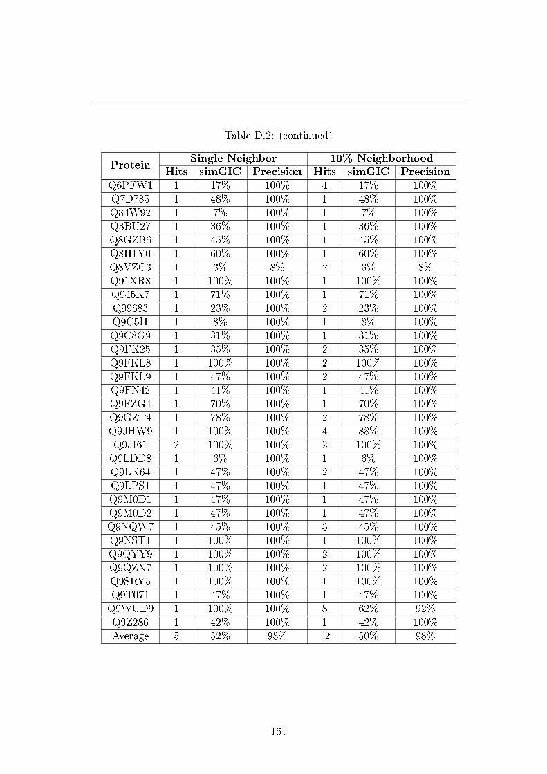
Table D.2: (continued)
ProteinSingle Neighbor 10% Neighborhood
Hits simGIC Precision Hits simGIC PrecisionQ6PFW1 1 17% 100% 4 17% 100%Q7D785 1 48% 100% 1 48% 100%Q84W92 1 7% 100% 1 7% 100%Q8BU27 1 36% 100% 1 36% 100%Q8GZB6 1 45% 100% 1 45% 100%Q8H1Y0 1 60% 100% 1 60% 100%Q8VZC3 1 3% 8% 2 3% 8%Q91XR8 1 100% 100% 1 100% 100%Q945K7 1 71% 100% 1 71% 100%Q99683 1 23% 100% 2 23% 100%Q9C5I1 1 8% 100% 1 8% 100%Q9C8G9 1 31% 100% 1 31% 100%Q9FK25 1 35% 100% 2 35% 100%Q9FKL8 1 100% 100% 2 100% 100%Q9FKL9 1 47% 100% 2 47% 100%Q9FN42 1 41% 100% 1 41% 100%Q9FZG4 1 70% 100% 1 70% 100%Q9GZT4 1 78% 100% 2 78% 100%Q9JHW9 1 100% 100% 4 88% 100%Q9JI61 2 100% 100% 2 100% 100%Q9LDD8 1 6% 100% 1 6% 100%Q9LK64 1 47% 100% 2 47% 100%Q9LPS1 1 47% 100% 1 47% 100%Q9M0D1 1 47% 100% 1 47% 100%Q9M0D2 1 47% 100% 1 47% 100%Q9NQW7 1 45% 100% 3 45% 100%Q9NST1 1 100% 100% 1 100% 100%Q9QYY9 1 100% 100% 2 100% 100%Q9QZX7 1 100% 100% 2 100% 100%Q9SRY5 1 100% 100% 1 100% 100%Q9T071 1 47% 100% 1 47% 100%Q9WUD9 1 100% 100% 8 62% 92%Q9Z286 1 42% 100% 1 42% 100%Average 5 52% 98% 12 50% 98%
161
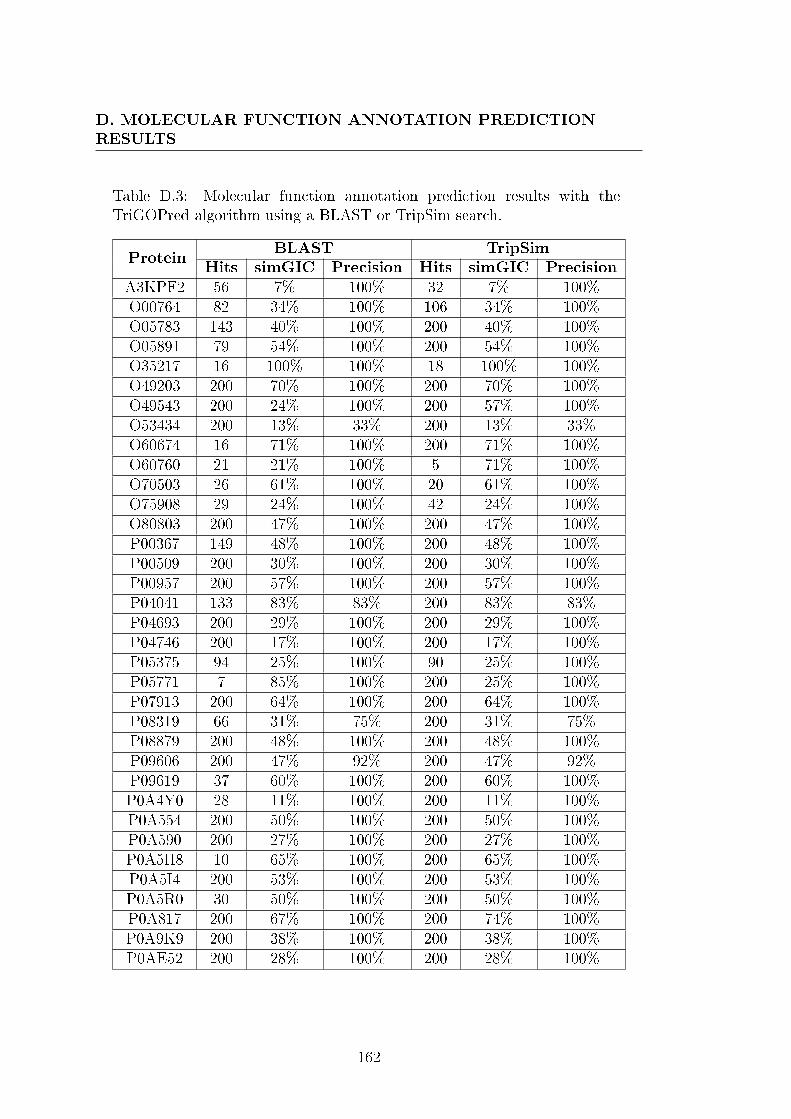
D. MOLECULAR FUNCTION ANNOTATION PREDICTIONRESULTS
Table D.3: Molecular function annotation prediction results with theTriGOPred algorithm using a BLAST or TripSim search.
ProteinBLAST TripSim
Hits simGIC Precision Hits simGIC PrecisionA3KPF2 56 7% 100% 32 7% 100%O00764 82 34% 100% 106 34% 100%O05783 143 40% 100% 200 40% 100%O05891 79 54% 100% 200 54% 100%O35217 16 100% 100% 18 100% 100%O49203 200 70% 100% 200 70% 100%O49543 200 24% 100% 200 57% 100%O53434 200 13% 33% 200 13% 33%O60674 16 71% 100% 200 71% 100%O60760 21 21% 100% 5 71% 100%O70503 26 61% 100% 20 61% 100%O75908 29 24% 100% 42 24% 100%O80803 200 47% 100% 200 47% 100%P00367 149 48% 100% 200 48% 100%P00509 200 30% 100% 200 30% 100%P00957 200 57% 100% 200 57% 100%P04041 133 83% 83% 200 83% 83%P04693 200 29% 100% 200 29% 100%P04746 200 17% 100% 200 17% 100%P05375 94 25% 100% 90 25% 100%P05771 7 85% 100% 200 25% 100%P07913 200 64% 100% 200 64% 100%P08319 66 31% 75% 200 31% 75%P08879 200 48% 100% 200 48% 100%P09606 200 47% 92% 200 47% 92%P09619 37 60% 100% 200 60% 100%P0A4Y0 28 11% 100% 200 11% 100%P0A554 200 50% 100% 200 50% 100%P0A590 200 27% 100% 200 27% 100%P0A5H8 10 65% 100% 200 65% 100%P0A5I4 200 53% 100% 200 53% 100%P0A5R0 30 50% 100% 200 50% 100%P0A817 200 67% 100% 200 74% 100%P0A9K9 200 38% 100% 200 38% 100%P0AE52 200 28% 100% 200 28% 100%
162
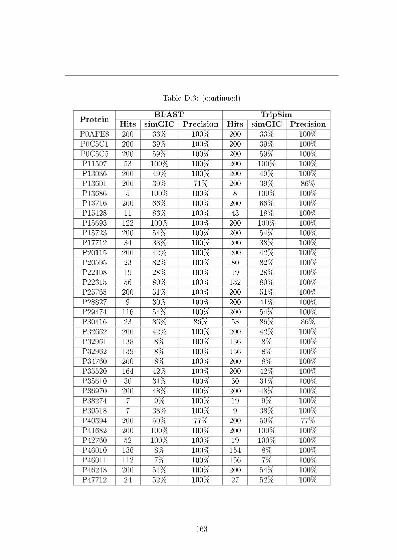
Table D.3: (continued)
ProteinBLAST TripSim
Hits simGIC Precision Hits simGIC PrecisionP0AFE8 200 33% 100% 200 33% 100%P0C5C1 200 39% 100% 200 39% 100%P0C5C5 200 59% 100% 200 59% 100%P11507 53 100% 100% 200 100% 100%P13086 200 49% 100% 200 49% 100%P13601 200 39% 71% 200 39% 86%P13686 5 100% 100% 8 100% 100%P13716 200 66% 100% 200 66% 100%P15428 11 83% 100% 43 18% 100%P15693 122 100% 100% 200 100% 100%P15723 200 54% 100% 200 54% 100%P17712 34 38% 100% 200 38% 100%P20115 200 42% 100% 200 42% 100%P20595 23 82% 100% 80 82% 100%P22108 19 28% 100% 19 28% 100%P22315 56 80% 100% 132 80% 100%P25765 200 51% 100% 200 51% 100%P28827 9 30% 100% 200 41% 100%P29474 116 54% 100% 200 54% 100%P30416 23 86% 86% 53 86% 86%P32662 200 42% 100% 200 42% 100%P32961 138 8% 100% 136 8% 100%P32962 139 8% 100% 156 8% 100%P34760 200 8% 100% 200 8% 100%P35520 164 42% 100% 200 42% 100%P35610 30 31% 100% 30 31% 100%P36970 200 48% 100% 200 48% 100%P38274 7 9% 100% 19 9% 100%P39518 7 38% 100% 9 38% 100%P40394 200 50% 77% 200 50% 77%P41682 200 100% 100% 200 100% 100%P42760 52 100% 100% 19 100% 100%P46010 136 8% 100% 154 8% 100%P46011 112 7% 100% 156 7% 100%P46248 200 54% 100% 200 54% 100%P47712 24 52% 100% 27 52% 100%
163
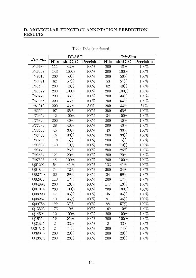
D. MOLECULAR FUNCTION ANNOTATION PREDICTIONRESULTS
Table D.3: (continued)
ProteinBLAST TripSim
Hits simGIC Precision Hits simGIC PrecisionP49186 111 48% 100% 200 48% 100%P49448 148 100% 100% 200 100% 100%P49615 200 50% 100% 200 50% 100%P50521 62 57% 100% 53 57% 100%P51433 200 48% 100% 62 48% 100%P51647 200 100% 100% 200 100% 100%P60479 200 33% 100% 200 33% 100%P61086 200 53% 100% 200 53% 100%P64012 200 33% 87% 200 33% 87%P66930 97 65% 100% 200 65% 100%P70352 12 100% 100% 34 100% 100%P75820 200 40% 100% 200 40% 100%P77489 28 40% 100% 200 40% 100%P78536 45 30% 100% 43 30% 100%P83483 46 83% 100% 200 83% 100%P83734 118 5% 100% 200 5% 100%P93834 140 70% 100% 200 70% 100%P96420 11 26% 100% 200 26% 100%P96864 121 20% 100% 200 20% 100%P97523 48 100% 100% 200 100% 100%Q01292 54 41% 100% 133 41% 100%Q01814 74 72% 100% 200 84% 100%Q02759 80 69% 100% 34 69% 100%Q02972 110 17% 100% 200 17% 100%Q04894 200 13% 100% 177 13% 100%Q07014 200 100% 100% 200 100% 100%Q08220 47 35% 100% 45 35% 100%Q08257 49 36% 100% 91 36% 100%Q09756 122 57% 100% 98 57% 100%Q13526 176 19% 100% 162 19% 100%Q14694 10 100% 100% 200 100% 100%Q16512 19 91% 100% 200 100% 100%Q21815 2 33% 100% 2 33% 100%Q2LAE1 2 74% 100% 200 74% 100%Q38946 200 20% 100% 200 20% 100%Q43314 200 23% 100% 200 23% 100%
164

Table D.3: (continued)
ProteinBLAST TripSim
Hits simGIC Precision Hits simGIC PrecisionQ56XE8 127 47% 100% 200 47% 100%Q5EAF2 16 17% 62% 15 17% 62%Q60587 59 100% 100% 81 100% 100%Q62658 200 56% 100% 200 56% 100%Q62689 17 57% 100% 200 100% 100%Q62925 13 34% 100% 200 33% 100%Q64428 200 100% 100% 200 100% 100%Q66HA1 33 100% 100% 200 100% 100%Q6PFW1 16 17% 100% 200 17% 100%Q7D785 16 48% 100% 200 48% 100%Q84W92 57 7% 100% 26 7% 100%Q8BU27 15 36% 100% 14 36% 100%Q8GZB6 20 45% 100% 19 45% 100%Q8H1Y0 200 60% 100% 200 60% 100%Q8VZC3 7 3% 8% 7 3% 8%Q91XR8 187 100% 100% 200 100% 100%Q945K7 200 71% 100% 200 71% 100%Q99683 11 25% 100% 200 23% 100%Q9C5I1 23 8% 100% 50 8% 100%Q9C8G9 25 31% 100% 200 31% 100%Q9FK25 200 35% 100% 200 35% 100%Q9FKL8 200 47% 100% 200 47% 100%Q9FKL9 200 47% 100% 200 47% 100%Q9FN42 200 41% 100% 200 41% 100%Q9FZG4 130 70% 100% 200 70% 100%Q9GZT4 200 78% 100% 199 78% 100%Q9JHW9 200 100% 100% 200 100% 100%Q9JI61 10 100% 100% 10 100% 100%Q9LDD8 200 6% 100% 200 6% 100%Q9LK64 3 47% 100% 200 47% 100%Q9LPS1 122 47% 100% 197 47% 100%Q9M0D1 200 47% 100% 200 47% 100%Q9M0D2 200 47% 100% 200 47% 100%Q9NQW7 200 45% 100% 199 45% 100%Q9NST1 13 100% 100% 13 100% 100%Q9QYY9 11 100% 100% 200 100% 100%
165
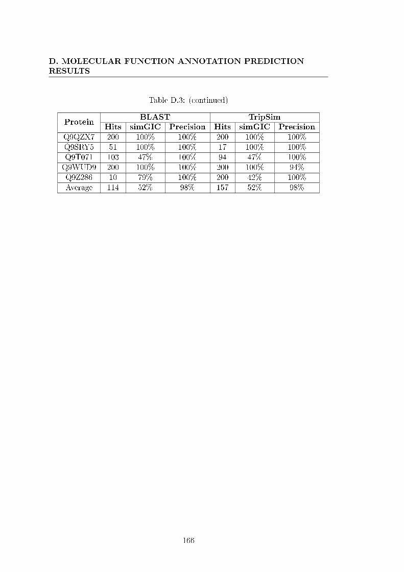
D. MOLECULAR FUNCTION ANNOTATION PREDICTIONRESULTS
Table D.3: (continued)
ProteinBLAST TripSim
Hits simGIC Precision Hits simGIC PrecisionQ9QZX7 200 100% 100% 200 100% 100%Q9SRY5 51 100% 100% 17 100% 100%Q9T071 103 47% 100% 94 47% 100%Q9WUD9 200 100% 100% 200 100% 94%Q9Z286 10 79% 100% 200 42% 100%Average 114 52% 98% 157 52% 98%
166

References
Akbani, R., Kwek, S. & Japkowicz, N. (2004). Applying support vec-
tor machines to imbalanced datasets. In ECML, 39�50.
Al-Shahib, A., Breitling, R. & Gilbert, D. (2007). Predicting pro-
tein function by machine learning on amino acid sequences - a critical
evaluation. BMC Genomics , 8, 78.
Alterovitz, G., Xiang, M., Hill, D.P., Lomax, J., Liu, J.,
Cherkassky, M., Dreyfuss, J., Mungall, C., Harris, M.A.,
Dolan, M.E., Blake, J.A. & Ramoni, M.F. (2010). Ontology en-
gineering. Nat Biotechnol , 28, 128�130.
Altschul, S.F., Gish, W., Miller, W., Myers, E.W. & Lipman,
D.J. (1990). Basic local alignment search tool. J Mol Biol , 215, 403�
410.
Altschul, S.F., Madden, T.L., Schäffer, A.A., Zhang, J., Zhang,
Z., Miller, W. & Lipman, D.J. (1997). Gapped blast and psi-blast: a
new generation of protein database search programs. Nucleic Acids Res ,
25, 3389�3402.
Apweiler, R., Bairoch, A. & Wu, C.H. (2004). Protein sequence
databases. Curr Op Chem Biol , 8, 76�80.
Avery, O.T., Macleod, C.M. & McCarty, M. (1944). Studies on the
chemical nature of the substance inducing transformation of pneumo-
coccal types: Induction of transformation by a desoxyribonucleic acid
fraction isolated from pneumococcus type iii. J Exp Med , 79, 137�158.
167
REFERENCES
Bada, M., Turi, D., McEntire, R. & Stevens, R. (2004). Using
reasoning to guide annotation with gene ontology terms in goat. SIGMOD
Rec, 33, 27�32.
Bairoch, A. (2000). The enzyme database in 2000. Nucleic Acids Res , 28,
304�305.
Barrell, D., Dimmer, E., Huntley, R.P., Binns, D., O'Donovan,
C. & Apweiler, R. (2009). The goa database in 2009-an integrated
gene ontology annotation resource. Nucleic Acids Res , 37, D396�D403.
Ben-Hur, A. & Weston, J. (2008). A user's guide to support vector
machines. In O. Carugo & F. Eisenhaber, eds., Data Mining Techniques
for the Life Sciences , vol. 609 of Methods in Molecular Biology , 223�239,
Humana Press.
Berman, H.M., Henrick, K. & Nakamura, H. (2003). Announcing
the worldwide protein data bank. Nat Struct Biol , 10, 980.
Bhardwaj, N., Langlois, R.E., Zhao, G. & Lu, H. (2005). Kernel-
based machine learning protocol for predicting DNA-binding proteins.
Nucleic Acids Res , 33, 6486�6493.
Bodenreider, O., Aubry, M. & Burgun, A. (2005). Non-lexical ap-
proaches to identifying associative relations in the Gene Ontology. 91�
102.
Brodley, C.E. & Friedl, M.A. (1999). Identifying mislabeled training
data. J Artif Intell Res , 11, 131�167.
Cai, C., Han, L., Ji, Z. & Chen, Y. (2004). Enzyme family classi�cation
by support vector machines. Proteins , 55, 66�76.
Camon, E.B., Barrell, D.G., Dimmer, E.C., Lee, V., Magrane,
M., Maslen, J., Binns, D. & Apweiler, R. (2005). An evaluation of
GO annotation retrieval for BioCreAtIvE and GOA. BMC Bioinformat-
ics , 6, S17.
168
REFERENCES
Chou, K.C. (2001). Prediction of protein cellular attributes using pseudo-
amino acid composition. Proteins , 43, 246�255.
Conesa, A., Götz, S., Garcia-Gomez, J.M., Terol, J., Talon, M.
& Robles, M. (2005). Blast2go: a universal tool for annotation, visual-
ization and analysis in functional genomics research. Bioinformatics , 21,
3674�3676.
Couto, F., Silva, M.J. & Coutinho, P. (2007). Measuring semantic
similarity between gene ontology terms. Data Knowl Eng , 61, 137�152.
Crick, F.H., Barnett, L., Brenner, S. & Watts-Tobin, R.J. (1961).
General nature of the genetic code for proteins. Nature, 192, 1227�1232.
Devos, D. & Valencia, A. (2000). Practical limits of function prediction.
Proteins , 41, 98�107.
Devos, D. & Valencia, A. (2001). Intrinsic errors in genome annotation.
Trends Genet , 17, 429�431.
Dolan, M.E., Ni, L., Camon, E. & Blake, J.A. (2005). A procedure
for assessing GO annotation consistency. Bioinformatics , 21, i136�i143.
Dubchak, I., Muchnik, I., H, S.R.H.S. & Kim (1995). Prediction of
protein folding class using global description of amino acid sequence. Proc
Natl Acad Sci , 92, 8700�8704.
Falcao, A.O. (2005). Residue fragment programs for enzyme classi�ca-
tion. In Bioinformatics: Knowledge Discovery in Biology , 24�28.
Falcao, A.O., Faria, D. & Ferreira, A. (2008). Peptide programs:
Applying fragment programs to protein classi�cation. In DTMBIO'08:
Proceedings of the 2008 ACM 2nd CIKM workshop on Data and Text
Mining Methods in Bioinformatics .
Faria, D., Pesquita, C., Couto, F. & Falcao, A.O. (2007). Pro-
teinon: A web tool for protein semantic similarity. Tech. Rep. TR07-6,
Department of Informatics, Faculty of Sciences, University of Lisbon.
169
REFERENCES
Feng, Z.P. & Zhang, C.T. (2000). Prediction of membrane protein types
based on the hydrophobic index of amino acids. J Protein Chem, 19, 262�
275.
Finn, R.D., Tate, J., Mistry, J., Coggill, P.C., Sammut, J.S.,
Hotz, H.R., Ceric, G., Forslund, K., Eddy, S.R., Sonnhammer,
E.L. & Bateman, A. (2008). The pfam protein families database. Nu-
cleic Acids Res , 36, D281�D288.
Friedberg, I. (2006). Automated protein function prediction - the ge-
nomic challenge. Brief Bioinform, 7, 225 �242.
Garg, A. & Gupta, D. (2008). VirulentPred: a SVM based prediction
method for virulent proteins in bacterial pathogens. BMC Bioinformat-
ics , 9, 62.
Gentleman (2005). Manual for R.
Han, J. & Kamber, M. (2006). Data Mining: Concepts and Techniques .
Elsevier.
Han, L., Cui, J., Lin, H., Ji, Z., Cao, Z., Li, Y. & Chen, Y. (2006).
Recent progresses in the application of machine learning approach for
predicting protein functional class independent of sequence similarity.
Proteomics , 6, 4023�4037.
Han, L.Y., Cai, C.Z., Ji, Z.L., Cao, Z.W., Cui, J. & Chen, Y.Z.
(2004). Predicting functional family of novel enzymes irrespective of se-
quence similarity: a statistical learning approach. Nucleic Acids Res , 32,
6437�6444.
Hawkins, T., Chitale, M., Luban, S. & Kihara, D. (2009). PFP:
automated prediction of gene ontology functional annotations with con-
�dence scores using protein sequence data. Proteins , 74, 566�582.
Hughey, R. & Krogh, A. (1996). Hidden markov models for sequence
analysis: extension and analysis of the basic method. Comput Appl
Biosci , 12, 95�107.
170

REFERENCES
Hulo, N., Bairoch, A., Bulliard, V., Cerutti, L., de Castro, E.,
Langendijk-Genevaux, P.S., Pagni, M. & Sigrist, C.J.A. (2006).
The prosite database. Nucleic Acids Res , 34, D227�D230.
Hunter, S., Apweiler, R., Attwood, T.K., Bairoch, A., Bate-
man, A., Binns, D., Bork, P., Das, U., Daugherty, L.,
Duquenne, L., Finn, R.D., Gough, J., Haft, D., Hulo, N., Kahn,
D., Kelly, E., Laugraud, A., Letunic, I., Lonsdale, D., Lopez,
R., Madera, M., Maslen, J., McAnulla, C., McDowall, J.,
Mistry, J., Mitchell, A., Mulder, N., Natale, D., Orengo,
C., Quinn, A.F., Selengut, J.D., Sigrist, C.J.A., Thimma, M.,
Thomas, P.D., Valentin, F., Wilson, D., Wu, C.H. & Yeats,
C. (2009). InterPro: the integrative protein signature database. Nucleic
Acids Research, 37, D211�215.
International Human Genome Sequencing Consortium (2004).
Finishing the euchromatic sequence of the human genome. Nature, 431,
931�945.
Jain, P., Wadhwa, P., Aygun, R. & Podila, G. (2008). Vector-G:
multi-modular SVM-based heterotrimeric g protein prediction. In Silico
Biol , 8, 141�155.
Jeffery, C.J. (1999). Moonlighting proteins. Trends Biochem Sci , 24,
8�11.
Jiang, J. & Conrath, D. (1997). Semantic similarity based on corpus
statistics and lexical taxonomy. In Proc of the 10th International Confer-
ence on Research on Computational Linguistics .
Joachims, T. (1999). Making large-Scale SVM Learning Practical . MIT-
Press.
Jones, C.E., Brown, A.L. & Baumann, U. (2007). Estimating the
annotation error rate of curated go database sequence annotations. BMC
Bioinformatics , 8, 170.
171

REFERENCES
Karp, P.D. (1998). What we do not know about sequence analysis and
sequence databases. Bioinformatics , 14, 753�754.
King, R.D., Karwath, A., Clare, A. & Dehaspe, L. (2000). Acurate
prediction of protein functional class from sequence in the m. tuberculosis
and e. coli genomes using data mining. Yeast , 17, 283�293.
Kirkpatrick, S., Gelatt, C.D. & Vecchi, M.P. (1983). Optimization
by simulated annealing. Science, 13, 671�680.
Kumar, A., Smith, B. & Borgelt, C. (2004). Dependence relationships
between gene ontology terms based on TIGR gene product annotations.
In CompuTerm, 31�38.
Kumar, M., Gromiha, M. & Raghava, G. (2007). Identi�cation of dna-
binding proteins using support vector machines and evolutionary pro�les.
BMC Bioinformatics , 8, 463.
Langlois, R., Carson, M., Bhardwaj, N. & Lu, H. (2007). Learning
to translate sequence and structure to function: Identifying dna binding
and membrane binding proteins. Ann Biomed Eng , 35, 1043�1052.
Leonelli, S., Diehl, A.D., Christie, K.R., Harris, M.A. & Lomax,
J. (2011). How the gene ontology evolves. BMC Bioinformatics , 12, 325.
Li, Z.R., Lin, H.H., Han, L.Y., Jiang, L., Chen, X. & Chen, Y.Z.
(2006). Profeat: A web server for computing structural and physicochem-
ical features of proteins and peptides from amino acid sequence. Nucleic
Acids Res , 34, W32�37.
Liao, B., Jiang, J., Zeng, Q. & Zhu, W. (2011). Predicting apoptosis
protein subcellular location with PseAAC by incorporating tripeptide
composition. Protein Peptide Lett , 18, 1086�1092.
Lin, D. (1998). An information-theoretic de�nition of similarity. In Proc of
the 15th International Conference on Machine Learning , 296�304.
172

REFERENCES
Lin, H., Han, L., Zhang, H., Zheng, C., Xie, B., Cao, Z. & Chen, Y.
(2006). Prediction of the functional class of metal-binding proteins from
sequence derived physicochemical properties by support vector machine
approach. BMC Bioinformatics , 7, S13.
Lord, P., Stevens, R., Brass, A. & Goble, C. (2003). Investigating
semantic similarity measures across the Gene Ontology: the relationship
between sequence and annotation. Bioinformatics , 19, 1275�1283.
Martin, D.M., Berriman, M. & Barton, G.J. (2004). Gotcha: a new
method for prediction of protein function assessed by the annotation of
seven genomes. BMC Bioinformatics , 5, 178.
Mathies, R.A. & Huang, X.C. (1992). Capillary array electrophoresis:
An approach to high-speed, high-throughput dna sequencing. Nature,
359, 167�169.
Mishra, N.K., Kumar, M. & Raghava, G.P.S. (2007). Support vector
machine based prediction of glutathione s-transferase proteins. Protein
Peptide Lett , 14, 575�580.
Mungall, C.J., Bada, M., Berardini, T.Z., Deegan, J., Ireland,
A., Harris, M.A., Hill, D.P. & Lomax, J. (2011). Cross-product
extensions of the gene ontology. J Biomed Inform, 44, 80�86.
Ong, S.A.K., Lin, H.H., Chen, Y.Z., Li, Z.R. & Cao, Z. (2007).
E�cacy of di�erent protein descriptors in predicting protein functional
families. BMC Bioinformatics , 8, 300.
Pasquier, C., Promponas, V.J. & Hamodrakas, S.J. (2001). Pred-
class: Cascading neural networks for generalized protein classi�cation and
genome-wide applications. Proteins , 44, 361�369.
Pellegrini, M., Marcotte, E.M., Thompson, M.J., Eisenberg, D.
& Yeates, T.O. (1999). Assigning protein functions by comparative
genome analysis: protein phylogenetic pro�les. Proc Natl Acad Sci , 96,
4285�4288.
173
REFERENCES
Resnik, P. (1999). Semantic similarity in a taxonomy: an information-
based measure and its application to problems of ambiguity in natural
language. J Artif Intell Res , 11, 95�130.
Rost, B. (1999). Twilight zone of protein sequence alignments. Protein
Eng , 12, 85�94.
Rost, R.J. (2006). OpenGL Shading Language. Addison and Wesley Pro-
fessional.
Saiki, R.K., Gelfand, D.H., Stoffel, S., Scharf, S.J., Higuchi, R.,
Horn, G.T., Mullis, K.B. & Erlich, H.A. (1988). Primer-directed
enzymatic ampli�cation of dna with a thermostable dna polymerase. Sci-
ence, 239, 487�491.
Sanger, F., Nicklen, S. & Coulson, A.R. (1977). Dna sequencing
with chain-terminating inhibitors. Proc Natl Acad Sci , 74, 5463�5467.
Saraç, O.S., Atalay, V. & Cetin-Atalay, R. (2010). GOPred: GO
molecular function prediction by combined classi�ers. PloS One, 5,
e12382.
Scheer, M., Grote, A., Chang, A., Schomburg, I., Munaretto,
C., Rother, M., Söhngen, C., Stelzer, M., Thiele, J. & Schom-
burg, D. (2011). BRENDA, the enzyme information system in 2011.
Nucleic Acids Res , 39, D670�676.
Schena, M., Shalon, D., Davis, R.W. & Brown, P.O. (1995). Quan-
titative monitoring of gene expression patterns with a complementary
dna microarray. Science, 270, 467�470.
Schlicker, A. & Albrecht, M. (2010). FunSimMat update: new fea-
tures for exploring functional similarity. Nucleic Acids Res , 38, D244�
248.
Schlicker, A., Domingues, F.S., Rahnenführer, J. & Lengauer,
T. (2006). A new measure for functional similarity of gene products based
on gene ontology. BMC Bioinformatics , 7.
174
REFERENCES
Söding, J. (2005). Protein homology detection by hmm-hmm comparison.
Bioinformatics , 21, 951�960.
Sokolov, A. & Ben-Hur, A. (2010). Hierarchical classi�cation of gene
ontology terms using the GOstruct method. J Bioinform Comput Biol ,
8, 357�376.
Srikant, R. & Agrawal, R. (1995). Mining generalized association rules.
Tech. Rep. RJ 9963, IBM Almaden Research.
The Gene Ontology Consortium (2000). Gene ontology: tool for the
uni�cation of biology. Nature Genet , 25, 25�29.
The Gene Ontology Consortium (2012). The gene ontology: enhance-
ments for 2011. Nucleic Acids Res , 40, D559�564.
The UniProt Consortium (2010). The universal protein resource
(UniProt) in 2010. Nucleic Acids Res , 38, D142�148.
Tian, W. & Skolnick, J. (2003). How well is enzyme function conserved
as a function of pairwise sequence identity. J Mol Biol , 333, 863�882.
Watson, J.D. & Crick, F.H. (1953). Molecular structure of nucleic acids:
A structure for deoxyribose nucleic acid. Nature, 171, 737�738.
Webb, E.C. (1992). Enzyme nomenclature 1992: recommendations of the
Nomenclature Committee of the International Union of Biochemistry and
Molecular Biology on the nomenclature and classi�cation of enzymes..
Academic Press.
Whisstock, J.C. & Lesk, A.M. (2003). Prediction of protein function
from protein sequence and structure. Q Rev Biophys , 36, 307�340.
Yang, M.Q., Yang, J.Y. & Ersoy, O.K. (2007). Classi�cation of pro-
teins multiple-labelled and single-labelled with protein functional classes.
Int J Gen Syst , 36, 91�109.
175

REFERENCES
Yang, Z.R. & Hamer, R. (2007). Bio-basis function neural networks in
protein data mining. Curr Pharm Design, 13, 1403�1413.
Zhang, Y. (2008). Progress and challenges in protein structure prediction.
Curr Opin Struct Biol , 18, 342�348.
176