Embed Size (px)
Citation preview

B0 → DK*0崩壊の研究
東北大学
根岸 健太郎
1
©H.Nakano
11/12/06 Bワークショップ @ 磐梯熱海
目次
• 序論 – Belle実験 – CP非保存角φ3
– B → DK崩壊
• RDK*測定
• まとめ
2
序論
Belle実験について CP非保存角φ3とは
φ3測定のためのB → DK崩壊
3

µ / KL detection
CsI(Tl)
Aerogel Cherenkov cnt.
Si vtx. det.
TOF conter
8 GeV e-
3.5 GeV e+
Central Drift Chamber
Belle実験 • Belle実験
– e+e-衝突でΥ(4S)(bbレゾナンス)を生成
• KEKB加速器 – e- : 8.0 GeV, e+ 3.5 GeV, 重心エネルギー10.6 GeV (非線形) – e+e-衝突器として世界最高のルミノシティ
• Belle検出器
Υ(4S) → B+B- ~ 50 % → B0B0 ~ 50 %
__
4

CP非保存角φ3
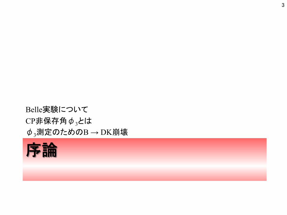
• CKM(Caibbo-小林-益川)行列 ‒ 弱い相互作用のCharged currentに入ってくる行列 ‒ 質量の固有状態とフレイバーの固有状態を混合
U = (u, c, t) D = (d, s, b) UL, DL : 左巻き成分
Lint = − g√2(ULγµVCKMDLW+
µ ) + h.c.
W
D
U
5

CP非保存角φ3
• CKM(Caibbo-小林-益川)行列 ‒ 弱い相互作用のCharged currentに入ってくる行列 ‒ 質量の固有状態とフレイバーの固有状態を混合
– CKM行列はユニタリでなければならない
U = (u, c, t) D = (d, s, b) UL, DL : 左巻き成分
Lint = − g√2(ULγµVCKMDLW+
µ ) + h.c.
VCKM =
Vud Vus Vub
Vcd Vcs Vcb
Vtd Vts Vtb
VCKMV †CKM = 1
ユニタリ条件
各成分は複素数 複素位相はVub, Vtdに押し込める事が出来る
6
CP非保存角φ3
• CKM(Caibbo-小林-益川)行列 ‒ 弱い相互作用のCharged currentに入ってくる行列 ‒ 質量の固有状態とフレイバーの固有状態を混合
– CKM行列はユニタリでなければならない
‒ 各項が複素数 → 複素平面上に三角形 → ユニタリ三角形
U = (u, c, t) D = (d, s, b) UL, DL : 左巻き成分
Lint = − g√2(ULγµVCKMDLW+
µ ) + h.c.
VCKM =
Vud Vus Vub
Vcd Vcs Vcb
Vtd Vts Vtb
VCKMV †CKM =
1 0 00 1 00 0 1
VudV∗ub + VcdV
∗cb + VtdV
∗tb = 0
7

ユニタリ三角形
• ユニタリ三角形
• b → u遷移のある(Vubの含まれる)モードで観測する事となる。 ‒ どのように観測するか → 次ページ
φ3の精度が悪い 精度の向上 → SMパラメターの精密測定 → New Physicsの手掛かり?
φ1
φ2
φ3
VudV∗ub
VcdV∗cb
VtdV∗tb
φ1 = (21.15+0.90−0.88)
◦
φ2 = (89.0+4.4−4.2)
◦
φ3 = (68+13−14)
◦
φ3 ≡ arg�
VudV ∗ub
−VcdV ∗cb
�
∼ − arg(Vub)
8
ICHEP 2010 EPS 2011

φ3測定とB → DK崩壊
• D0, D0が同じ終状態 f へ崩壊 ‒ 終状態が同じ二つのtree diagramが干渉
• 経路Aにb → u遷移が含まれる → φ3の影響が入ってくる
D : D0 or D0
b
u
u
u
c
s
W
Vub
_ _
_
B-
D0 → f
K-
φ3の情報 _
_
経路A
b
u
u
u
s
c
W
_ _
_
B-
D0 → f
K-
経路B
9
_
かなりざっくりした説明↑ 勿論他にも色々効果が入って来る訳で、、、 もう少し具体的に、 • どんな観測量を測るのか? • どんな f を使うの?

φ3測定とB → DK崩壊
• Charge conjugateで弱い相互作用の位相は符号が反転する。 • 経路A,B間でに異なる強い相互作用の位相δが入ってくる
• 観測されるのは赤い線の(経路A,Bの干渉を経た)二乗
D : D0 or D0
b
u
u
u
c
s
W
Vub
_ _
_
B-
D0 → f
K-
φ3の情報 _
_
経路A
b
u
u
u
s
c
W
_ _
_
B-
D0 → f
K-
経路B
経路B
経路A = 経路A
_____
経路B _____
δ + φ3
δ - φ3 δは符号反転しない
10
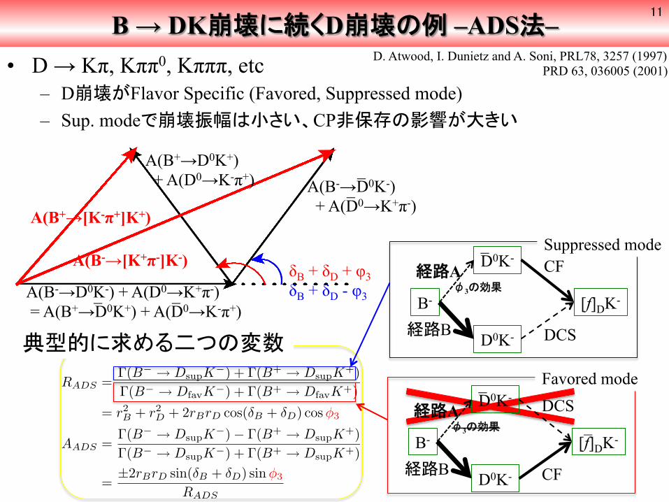
B → DK崩壊に続くD崩壊の例 –ADS法– • D → Kπ, Kππ0, Kπππ, etc
– D崩壊がFlavor Specific (Favored, Suppressed mode) – Sup. modeで崩壊振幅は小さい、CP非保存の影響が大きい
A(B-→D0K-) + A(D0→K+π-) = A(B+→D0K+) + A(D0→K-π+)
_ _
A(B+→D0K+) + A(D0→K-π+) A(B-→D0K-)
+ A(D0→K+π-)
_ _
A(B+→[K-π+]K+)
A(B-→[K+π-]K-) δB + δD + φ3 δB + δD - φ3
RADS =Γ(B− → DsupK−) + Γ(B+ → DsupK+)Γ(B− → DfavK−) + Γ(B+ → DfavK+)
= r2B + r2
D + 2rBrD cos(δB + δD) cos φ3
AADS =Γ(B− → DsupK−)− Γ(B+ → DsupK+)Γ(B− → DsupK−) + Γ(B+ → DsupK+)
=±2rBrD sin(δB + δD) sinφ3
RADS
典型的に求める二つの変数
11
D. Atwood, I. Dunietz and A. Soni, PRL78, 3257 (1997) PRD 63, 036005 (2001)
B-
D0K-
D0K-
[f]DK-
_ 経路A φ3の効果
経路B
CF
DCS
Favored mode
Suppressed mode
B-
D0K-
D0K-
[f]DK-
_ 経路A φ3の効果
経路B
DCS
CF
_
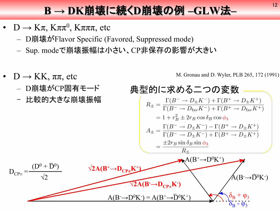
B → DK崩壊に続くD崩壊の例 –GLW法– • D → Kπ, Kππ0, Kπππ, etc
– D崩壊がFlavor Specific (Favored, Suppressed mode) – Sup. modeで崩壊振幅は小さい、CP非保存の影響が大きい
• D → KK, ππ, etc – D崩壊がCP固有モード ‒ 比較的大きな崩壊振幅
12
DCP± = √2
(D0 + D0) _ A(B+→D0K+)
A(B-→D0K-) _
A(B-→D0K-) = A(B+→D0K+) _
√2A(B+→DCP±K+)
√2A(B-→DCP±K-) δB + φ3 δB - φ3
R± =Γ(B− → D±K−) + Γ(B+ → D±K+)
Γ(B− → DfavK−) + Γ(B+ → DfavK+)= 1 + r2
B ± 2rB cos δB cos φ3
A± =Γ(B− → D±K−)− Γ(B+ → D±K+)Γ(B− → D±K−) + Γ(B+ → D±K+)
=±2rB sin δB sinφ3
R±
典型的に求める二つの変数
M. Gronau and D. Wyler, PLB 265, 172 (1991)

0
1000
2000
3000
4000
5000
6000
7000
0 0.5 1 1.5 2 2.5 3m2
(GeV2/c4)
Entr
ies/
0.02
GeV
2 /c4
(c) (d)
B → DK崩壊に続くD崩壊の例 –Dalitz plot analysis– • D → Kπ, Kππ0, Kπππ, etc
– D崩壊がFlavor Specific (Favored, Suppressed mode) – Sup. modeで崩壊振幅は小さい、CP非保存の影響が大きい
• D → KK, ππ, etc – D崩壊がCP固有モード ‒ 比較的大きな崩壊振幅
• D → KSππ, etc – D崩壊が三体崩壊 ‒ 三体崩壊のレゾナンス分布にφ3の影響が現れる
• 経由するレゾナンスにより強い相互作用の位相が異なる
A. Poluektov, PRL81, 112002 (2010)
φ3 = (78.4± 3.6(stat.)± 8.9(syst.)+11.6−10.8(model))◦
13
D*-→D0π-
D0→KSπ+π-
_ _

B → DKを用いたφ3測定
• D → Kπ, Kππ0, Kπππ, etc – D崩壊がFlavor Specific (Favored, Suppressed mode) – Sup. modeで崩壊振幅は小さい、CP非保存の影響が大きい
• D → KK, ππ, etc – D崩壊がCP固有モード ‒ 比較的大きな崩壊振幅
• D → KSππ, etc – D崩壊が三体崩壊 ‒ 三体崩壊のレゾナンス分布にφ3の影響が現れる
• 経由するレゾナンスにより強い相互作用の位相が異なる
• 全部ひっくるめて、連立方程式を作る事になるので、 他のモードを解析すればする程φ3の制限がかかる!
14
φ3の測定の一般的なお話オワリ、 次からは自分の研究したB0→DK*0について

B0 → DK*0
• Neutral Bを使うということは、、、
B0-B0 mixingの効果 (φ3以外の効果)が入ってきてしまう
15
頑張ろうとすると、 Δt, qr, …色々測らないといけない物が増える。
→ 大変
_

B0 → DK*0
• Neutral Bを使うということは、、、 B0-B0 mixingの効果(φ3以外の効果)が入ってきてしまう
– K*0によるSelf Taggingで解決
K*0 →
K+π- ~ 2/3 K0π0 ~ 1/3
16
OK!!
えらい楽
K+π-でK*を組んだ → K*0 → B0の崩壊 K-π+でK*を組んだ → K*0 → B0の崩壊
_ _
_

B0 → DK*0
• Neutral Bを使うということは、、、 B0-B0 mixingの効果(φ3以外の効果)が入ってきてしまう
– K*0によるSelf Taggingで解決
Charged Bの測定とは独立 干渉の効果が大きい
DKπ non-resonant modeの効果
• ここで求めるのは
b
d
u
d
c
s
W
_ _
_Vub
B0 _
D0 _
K*0 _
b
d
c
d
u
s
W
_ _
_
B0 _
D0
K*0 _
経路A, B共に Color Suppressed
K*0 → K+π- ~ 2/3 K0π0 ~ 1/3
RDK∗ ∼=Γ(B0 → [K+π−]DK∗0) + Γ(B0 → [K−π+]DK∗0)Γ(B0 → [K−π+]DK∗0) + Γ(B0 → [K+π−]DK∗0)
= r2S + r2
D + 2krSrD cos(δS + δD) cos φ3 Favored mode
Suppressed mode
17
OK!!
_
RDK*測定
B0 → [Kπ]D[Kπ]K*0
18
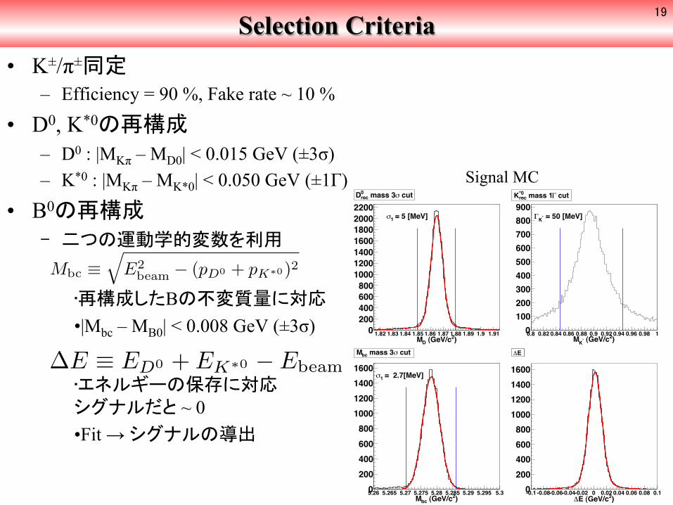
Selection Criteria • K±/π±同定
– Efficiency = 90 %, Fake rate ~ 10 %
• D0, K*0の再構成 – D0 : |MKπ – MD0| < 0.015 GeV (±3σ) – K*0 : |MKπ – MK*0| < 0.050 GeV (±1Γ)
• B0の再構成 ‒ 二つの運動学的変数を利用
• 再構成したBの不変質量に対応 • |Mbc – MB0| < 0.008 GeV (±3σ)
• エネルギーの保存に対応シグナルだと ~ 0 • Fit → シグナルの導出
Mbc ≡�
E2beam − (pD0 + pK∗0)2
∆E ≡ ED0 + EK∗0 − Ebeam
)2 (GeV/cDM1.82 1.83 1.84 1.85 1.86 1.87 1.88 1.89 1.9 1.910
200400600800
1000120014001600180020002200
= 5 [MeV]1
cut mass 3rec0D
)2 (GeV/c*KM0.8 0.82 0.84 0.86 0.88 0.9 0.92 0.94 0.96 0.98 10
100200300400500600700800900
= 50 [MeV]*K
cut mass 1rec*0K
)2 (GeV/cbcM5.26 5.265 5.27 5.275 5.28 5.285 5.29 5.295 5.30
200400600800
1000120014001600
= 2.7[MeV]1
cut mass 3bcM
)2E (GeV/c-0.1 -0.08-0.06-0.04-0.02 0 0.02 0.04 0.06 0.08 0.10
200400600800
1000120014001600
EE
19
Signal MC
)2 (GeV/c±K*0KM1.75 1.8 1.85 1.9 1.95 20
20
40
60
80
100
120
140
160
180
+-D0 B +-D0 B
)2 (GeV/c±K*0KM1.5 2 2.5 3 3.5 4 4.5 50
1000
2000
3000
4000
5000
6000
7000
Signal MC Signal MC
M0.12 0.13 0.14 0.15 0.16 0.17 0.18
Probability
0
0.01
0.02
0.03
0.04
0.05
0.06
0.07
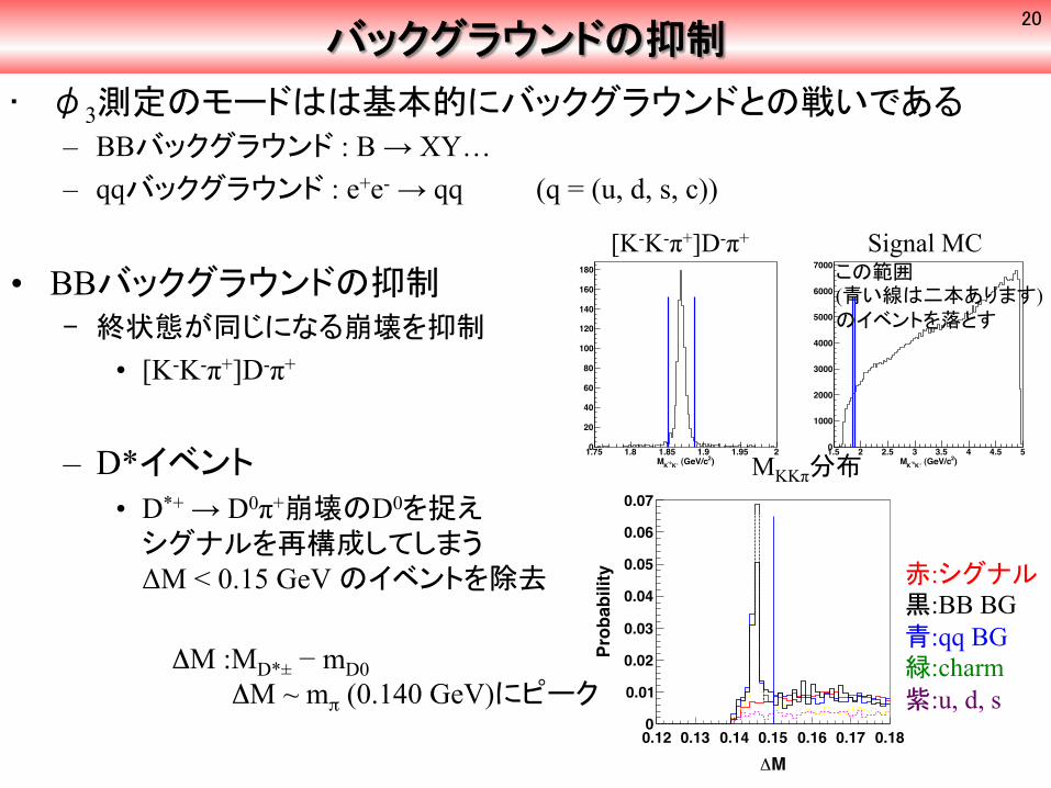
バックグラウンドの抑制
• φ3測定のモードはは基本的にバックグラウンドとの戦いである – BBバックグラウンド : B → XY… – qqバックグラウンド : e+e- → qq (q = (u, d, s, c))
• BBバックグラウンドの抑制 ‒ 終状態が同じになる崩壊を抑制
• [K-K-π+]D-π+
– D*イベント • D*+ → D0π+崩壊のD0を捉えシグナルを再構成してしまうΔM < 0.15 GeV のイベントを除去
ΔM :MD*± − mD0 ΔM ~ mπ (0.140 GeV)にピーク
赤:シグナル 黒:BB BG 青:qq BG 緑:charm 紫:u, d, s
20
[K-K-π+]D-π+ Signal MC
MKKπ分布
この範囲 (青い線は二本あります) のイベントを落とす
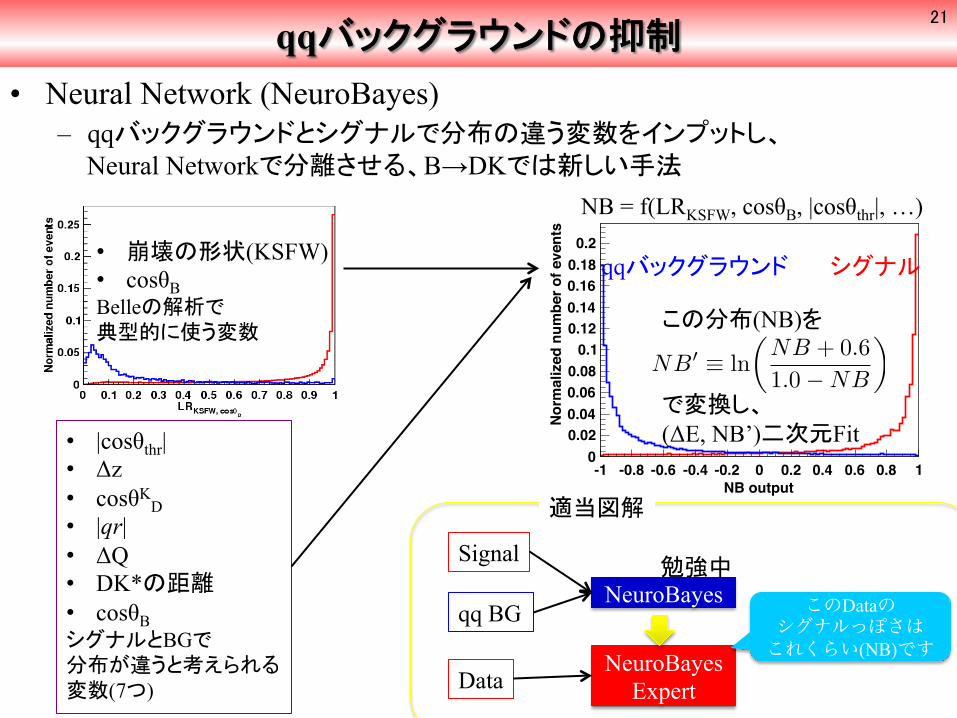
• 崩壊の形状(KSFW) • cosθB Belleの解析で 典型的に使う変数
qqバックグラウンドの抑制 • Neural Network (NeuroBayes)
– qqバックグラウンドとシグナルで分布の違う変数をインプットし、 Neural Networkで分離させる、B→DKでは新しい手法
• |cosθthr| • Δz • cosθK
D • |qr| • ΔQ • DK*の距離 • cosθB シグナルとBGで 分布が違うと考えられる 変数(7つ)
NB output
-1 -0.8 -0.6 -0.4 -0.2 0 0.2 0.4 0.6 0.8 1
No
rmalized
nu
mb
er
of
even
ts
0
0.02
0.04
0.06
0.08
0.1
0.12
0.14
0.16
0.18
0.2
シグナル qqバックグラウンド
この分布(NB)を で変換し、 (ΔE, NB’)二次元Fit
NB� ≡ ln�
NB + 0.61.0−NB
�
21
NB = f(LRKSFW, cosθB, |cosθthr|, …)
NeuroBayes
Signal
qq BG
勉強中
NeuroBayes Expert Data
このDataの シグナルっぽさは これくらい(NB)です
適当図解
E (GeV)-0.1 0 0.1 0.2 0.3
Even
ts /
( 0.0
1 )
0
5
10
15
20
25
30
E (GeV)-0.1 0 0.1 0.2 0.3
Even
ts /
( 0.0
1 )
0
5
10
15
20
25
30
NB’-10 -5 0 5 10
Even
ts /
( 0.4
)
05
1015202530354045
NB’-10 -5 0 5 10
Even
ts /
( 0.4
)
05
1015202530354045
E (GeV)-0.1 0 0.1 0.2 0.3
Even
ts /
( 0.0
1 )
0
10
20
30
40
50
E (GeV)-0.1 0 0.1 0.2 0.3
Even
ts /
( 0.0
1 )
0
10
20
30
40
50
NB’-10 -5 0 5 10
Even
ts /
( 0.4
)
0
5
10
15
20
25
30
35
40
NB’-10 -5 0 5 10
Even
ts /
( 0.4
)
0
5
10
15
20
25
30
35
40
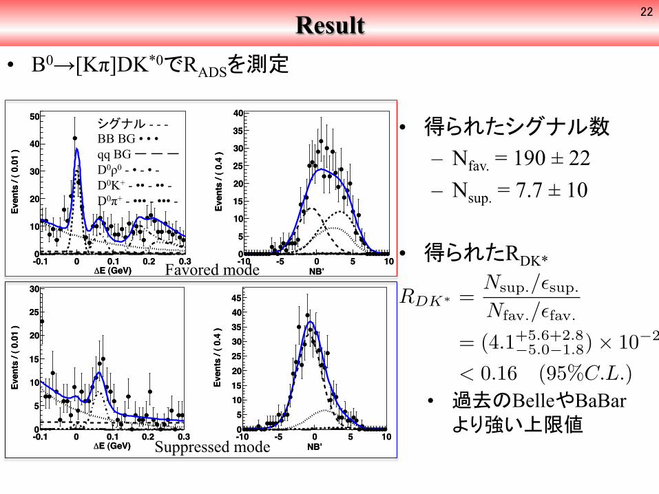
Result • B0→[Kπ]DK*0でRADSを測定
Favored mode
Suppressed mode
• 得られたシグナル数 – Nfav. = 190 ± 22 – Nsup. = 7.7 ± 10
• 得られたRDK*
• 過去のBelleやBaBarより強い上限値
RDK∗ =Nsup./�sup.
Nfav./�fav.
= (4.1+5.6+2.8−5.0−1.8)× 10−2
< 0.16 (95%C.L.)
22
シグナル - - - BB BG • • • qq BG ー ー ー D0ρ0 - • - • - D0Κ+ - •• - •• -
D0π+ - ••• - ••• -
まとめ
23

Summary and Plan • まとめ
– SMのパラメータの測定それ自体とても重要 • New Physicsの手掛かりとなる可能性
– Neutral Bでのφ3測定は未だ行われていない
• Charged Bでの結果とのクロスチェック
– B0→[Kπ]DK*0でのRDK*の上限値を更新する事に成功
• RDK* < 0.24 (95% C.L.) @BaBar 2009 with 465M BB < 0.16 (95% C.L.) @Belle My result with 772M BB
• ただいま論文を書いている所です。大変です。
• 今後の方針、課題 – B0→[KSππ]DK*0のDalitz解析 • 一生懸命頑張りたいと思います。
24

BACK UP
25

RDK* 26
RDK∗ ≡ Γ(B0 → [K+π−]DK + π−) + Γ(B0 → [K−π+]DK−π+)Γ(B0 → [K−π+]DK+π−) + Γ(B0 → [K+π−]DK−π+)
= r2S + r2
D + 2kkDrSrD cos(δS + δD) cos φ3
ADK∗ ≡ Γ(B0 → [K+π−]DK + π−)− Γ(B0 → [K−π+]DK−π+)Γ(B0 → [K+π−]DK+π−) + Γ(B0 → [K−π+]DK−π+)
=2kkDrSrD sin(δS + δD) sinφ3
RDK∗
r2S ≡
Γ(B0 → D0K+π−)Γ(B0 → D0K+π−)
=�
dpA2A(p)�
dpA2B(p)
keiδS ≡�
dpAA(p)AB(p)eiδ(p)
��dpA2
A(p)�
dpA2B(p)
r2D ≡
Γ(D0 → K+π−)Γ(D0 → K−π+)
=�
dmA2DCS(m)�
dmA2CF (m)
kDeiδD ≡�
dmADCS(m)ACF (m)eiδ(m)
��dmA2
DCS(m)�
dmA2CF (m)
他の実験で良く測定されている
B0→DK*0モードに特有

Neurobayes 27
Signal efficiency0 0.1 0.2 0.3 0.4 0.5 0.6 0.7 0.8 0.9 1
Bac
kgro
und
reje
ctio
n
0.2
0.3
0.4
0.5
0.6
0.7
0.8
0.9
1
Signal efficiency0 0.1 0.2 0.3 0.4 0.5 0.6 0.7 0.8 0.9 1
Bac
kgro
und
reje
ctio
n
0.2
0.3
0.4
0.5
0.6
0.7
0.8
0.9
1
LR0 0.1 0.2 0.3 0.4 0.5 0.6 0.7 0.8 0.9 1
Nor
mal
ized
num
ber o
f eve
nts
0
0.05
0.1
0.15
0.2
0.25
NB-1 -0.8 -0.6 -0.4 -0.2 0 0.2 0.4 0.6 0.8 1
Nor
mal
ized
num
ber o
f eve
nts
00.020.040.060.08
0.10.120.140.160.18
0.20.220.24
TRANSNB-10 -8 -6 -4 -2 0 2 4 6 8 10
Nor
mal
ized
num
ber o
f eve
nts
0
0.02
0.04
0.06
0.08
0.1
0.12
LR(KSFW, cosθB) NB(9 para.)

NeuroBayes training Phi-T
TeacherNeuroBayes
Training iteration20 40 60 80 100 120 140
arb.
uni
ts
0.004
0.002
0
0.002
0.004
0.006
0.008
Error
Training iteration20 40 60 80 100 120 140
arb.
uni
ts
0.006
0.004
0.002
0
0.002
0.004
0.006
Error Testsample
Training iteration20 40 60 80 100 120 140
arb.
uni
ts
0
.0002
.0004
.0006
.0008
0.001
.0012
regularisation param. * weights
Training iteration20 40 60 80 100 120 140
arb.
uni
ts
0.004
0.002
0
0.002
0.004
0.006
0.008
Err-Weight Learnsample
Phi-T TeacherNeuroBayes
Network output-1 -0.8 -0.6 -0.4 -0.2 0 0.2 0.4 0.6 0.8 1
even
ts
02000400060008000
100001200014000160001800020000
Output Node 1Output Node 1
Network output-1 -0.8 -0.6 -0.4 -0.2 0 0.2 0.4 0.6 0.8 1
purit
y
0
0.1
0.2
0.3
0.4
0.5
0.6
0.7
0.8
0.9
1
28
NeuroBayes training Phi-T
TeacherNeuroBayes
signal efficiency0 0.1 0.2 0.3 0.4 0.5 0.6 0.7 0.8 0.9 1
sign
al p
urity
0
0.1
0.2
0.3
0.4
0.5
0.6
0.7
0.8
0.9
1
efficiency0 0.1 0.2 0.3 0.4 0.5 0.6 0.7 0.8 0.9 1
sign
al e
ffici
ency
0
0.1
0.2
0.3
0.4
0.5
0.6
0.7
0.8
0.9
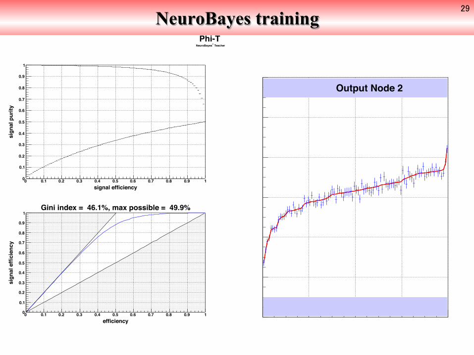
1Gini index = 46.1%, max possible = 49.9%
Phi-T TeacherNeuroBayes
0.5 25.5 50.5 75.5 100-0.1
0.1
0.3
0.5
0.7
0.9
1.1Output Node 2
29

NeuroBayes training
Phi-T TeacherNeuroBayes
0.5 25.5 50.5 75.5 100-0.1
0.1
0.3
0.5
0.7
0.9
1.1Output Node 2
Phi-T TeacherNeuroBayes
1 2 3 4 5 6 7 8 9 10
10
9
8
7
6
5
4
3
2
1
correlation matrix of input variables
-1 -0.8 -0.6 -0.4 -0.2 0 0.2 0.4 0.6 0.8 1
30

NeuroBayes training Phi-T
TeacherNeuroBayes
1 2 3 4 5 6 7 8 9 10 11
11
10
9
8
7
6
5
4
3
2
1
correlation matrix of input variables
-1 -0.8 -0.6 -0.4 -0.2 0 0.2 0.4 0.6 0.8 1
Phi-T TeacherNeuroBayes
Input node 2 : k0lrksfw PrePro: only this 274.32corr. to others 75.40%
1st most importantadded signi. 274.32signi. loss 89.69
0 0.2 0.4 0.6 0.8 1
even
ts
0200400600800
100012001400160018002000
flat
0.00411 0.0277 0.0356 0.0437 0.0512 0.0562 0.0626 0.0691 0.0771 0.0863 0.0968 0.1085555 0.1217634 0.1363846 0.1527715 0.1711791 0.1919617 0.21459 0.2408578 0.2707362 0.3036703 0.3386178 0.3780639 0.4206024 0.4670333 0.513757 0.5602144 0.6083206 0.6554167 0.7013494 0.7453929 0.7835921 0.8193789 0.8513414 0.8791555 0.9027795 0.9224075 0.9387981 0.9521092 0.9628142 0.9714955 0.9784776 0.984129 0.9885805 0.9918954 0.9947158 0.9967051 0.9981172 0.9991112 0.999761 1
bin #0 0.2 0.4 0.6 0.8 1
purit
y
0
0.2
0.4
0.6
0.8
1
purity
final netinput-3 -2 -1 0 1 2 3
even
ts
0
5001000
1500
20002500
3000
3500background
Underflow 1Overflow 61
backgroundUnderflow 1Overflow 61
final netinput-3 -2 -1 0 1 2 3
even
ts
0
5001000
1500
20002500
3000
3500background
Underflow 1Overflow 61
signalUnderflow 0Overflow 973
final
signal efficiency0 0.1 0.2 0.3 0.4 0.5 0.6 0.7 0.8 0.9 1
sign
al p
urity
0
0.2
0.4
0.6
0.8
1
separation
signal efficiency0 0.1 0.2 0.3 0.4 0.5 0.6 0.7 0.8 0.9 1
sign
al p
urity
0
0.2
0.4
0.6
0.8
1
separation31
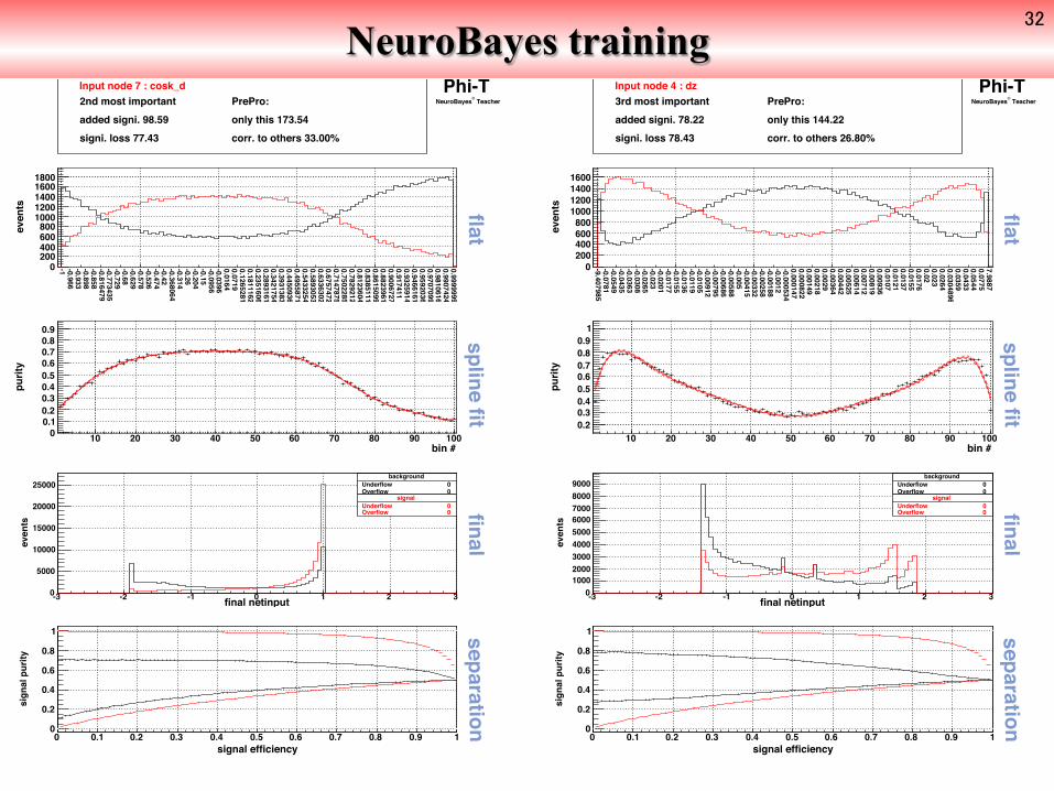
NeuroBayes training Phi-T
TeacherNeuroBayes
Input node 7 : cosk_d PrePro: only this 173.54corr. to others 33.00%
2nd most importantadded signi. 98.59signi. loss 77.43
0 0.2 0.4 0.6 0.8 1
even
ts
0200400600800
10001200140016001800
flat
-1 -0.966 -0.933 -0.898 -0.858 -0.816479 -0.773435 -0.729 -0.68 -0.629 -0.578 -0.526 -0.474 -0.42 -0.368064 -0.314 -0.26 -0.204 -0.15 -0.0956 -0.0396 0.0164 0.0719 0.1265281 0.1811162 0.2351606 0.2893161 0.3421754 0.3931383 0.4450936 0.4955871 0.5433254 0.5893053 0.6336302 0.6757472 0.7147875 0.7502285 0.7829212 0.8123604 0.8385111 0.8615099 0.8823961 0.9006727 0.917411 0.9325914 0.9466161 0.9592036 0.9707099 0.9810616 0.9907424 0.9999999
bin #10 20 30 40 50 60 70 80 90 100
purit
y
00.10.20.30.40.50.60.70.80.9 spline fit
final netinput-3 -2 -1 0 1 2 3
even
ts
0
5000
10000
15000
20000
25000background
Underflow 0Overflow 0
backgroundUnderflow 0Overflow 0
final netinput-3 -2 -1 0 1 2 3
even
ts
0
5000
10000
15000
20000
25000background
Underflow 0Overflow 0
signalUnderflow 0Overflow 0
final
signal efficiency0 0.1 0.2 0.3 0.4 0.5 0.6 0.7 0.8 0.9 1
sign
al p
urity
0
0.2
0.4
0.6
0.8
1
separation
signal efficiency0 0.1 0.2 0.3 0.4 0.5 0.6 0.7 0.8 0.9 1
sign
al p
urity
0
0.2
0.4
0.6
0.8
1
separation
Phi-T TeacherNeuroBayes
Input node 4 : dz PrePro: only this 144.22corr. to others 26.80%
3rd most importantadded signi. 78.22signi. loss 78.43
0 0.2 0.4 0.6 0.8 1
even
ts
0200400600800
1000120014001600
flat
-9.407985 -0.0781 -0.0549 -0.0435 -0.0363 -0.0308 -0.0265 -0.023 -0.0201 -0.0177 -0.0155 -0.0136 -0.0119 -0.0105 -0.00912 -0.00795 -0.00686 -0.00588 -0.005 -0.00415 -0.00332 -0.00258 -0.00188 -0.0012 -0.000534 0.000147 0.000822 0.00149 0.00218 0.0029 0.00364 0.00442 0.00525 0.00614 0.00712 0.00819 0.00936 0.0107 0.0121 0.0137 0.0155 0.0176 0.02 0.023 0.0264 0.0304896 0.0359 0.0433 0.0544 0.0775 7.9887
bin #10 20 30 40 50 60 70 80 90 100
purit
y
0.20.30.40.50.60.70.80.9
1 spline fit
final netinput-3 -2 -1 0 1 2 3
even
ts
0100020003000400050006000700080009000
backgroundUnderflow 0Overflow 0
backgroundUnderflow 0Overflow 0
final netinput-3 -2 -1 0 1 2 3
even
ts
0100020003000400050006000700080009000
backgroundUnderflow 0Overflow 0
signalUnderflow 0Overflow 0
final
signal efficiency0 0.1 0.2 0.3 0.4 0.5 0.6 0.7 0.8 0.9 1
sign
al p
urity
0
0.2
0.4
0.6
0.8
1
separation
signal efficiency0 0.1 0.2 0.3 0.4 0.5 0.6 0.7 0.8 0.9 1
sign
al p
urity
0
0.2
0.4
0.6
0.8
1
separation32
NeuroBayes training Phi-T
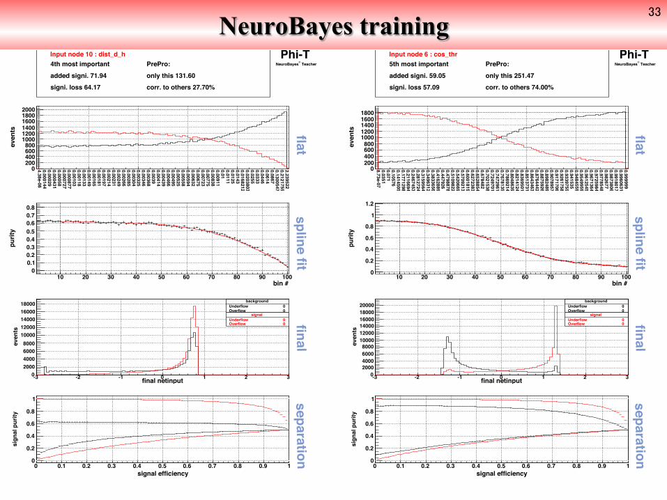
TeacherNeuroBayes
Input node 10 : dist_d_h PrePro: only this 131.60corr. to others 27.70%
4th most importantadded signi. 71.94signi. loss 64.17
0 0.2 0.4 0.6 0.8 1
even
ts
0200400600800
100012001400160018002000
flat
4.38e-08 0.000144 0.00029 0.000431 0.00058 0.000727 0.000877 0.00103 0.00118 0.00133 0.00149 0.00165 0.00181 0.00197 0.00214 0.00231 0.00249 0.00266 0.00285 0.00304 0.00325 0.00346 0.00368 0.0039 0.00414 0.00439 0.00466 0.00495 0.00525 0.00558 0.00594 0.00632 0.00675 0.00723 0.00775 0.00838 0.00911 0.01 0.0111 0.0125 0.0143 0.0168212 0.0203803 0.0255 0.0333 0.0446 0.0614 0.0867 0.1300547 0.2121755 2.239522
bin #10 20 30 40 50 60 70 80 90 100
purit
y
00.10.20.30.40.50.60.70.8 spline fit
final netinput-3 -2 -1 0 1 2 3
even
ts
02000400060008000
1000012000140001600018000 background
Underflow 0Overflow 0
backgroundUnderflow 0Overflow 0
final netinput-3 -2 -1 0 1 2 3
even
ts
02000400060008000
1000012000140001600018000 background
Underflow 0Overflow 0
signalUnderflow 0Overflow 0
final
signal efficiency0 0.1 0.2 0.3 0.4 0.5 0.6 0.7 0.8 0.9 1
sign
al p
urity
0
0.2
0.4
0.6
0.8
1
separation
signal efficiency0 0.1 0.2 0.3 0.4 0.5 0.6 0.7 0.8 0.9 1
sign
al p
urity
0
0.2
0.4
0.6
0.8
1
separation
Phi-T TeacherNeuroBayes
Input node 6 : cos_thr PrePro: only this 251.47corr. to others 74.00%
5th most importantadded signi. 59.05signi. loss 57.09
0 0.2 0.4 0.6 0.8 1
even
ts
0200400600800
10001200140016001800
flat
8.73e-07 0.0351 0.071 0.10576 0.1414505 0.1771298 0.2116694 0.2467453 0.2812724 0.3159564 0.3496312 0.3833656 0.4162889 0.447926 0.4798878 0.5109822 0.5420669 0.5709213 0.6001819 0.6272383 0.6528854 0.678482 0.7021538 0.7249701 0.7472961 0.7678135 0.7869214 0.8048639 0.8214124 0.8369501 0.8513731 0.8643463 0.8764442 0.8875926 0.8982489 0.9078957 0.9171706 0.9261758 0.9339755 0.941535 0.9484559 0.9549959 0.9612545 0.9671364 0.9725984 0.9778548 0.982677 0.9873806 0.9918017 0.9960631 0.999999
bin #10 20 30 40 50 60 70 80 90 100
purit
y
0
0.2
0.4
0.6
0.8
1
1.2 spline fit
final netinput-3 -2 -1 0 1 2 3
even
ts
02000400060008000
100001200014000160001800020000
backgroundUnderflow 0Overflow 0
backgroundUnderflow 0Overflow 0
final netinput-3 -2 -1 0 1 2 3
even
ts
02000400060008000
100001200014000160001800020000
backgroundUnderflow 0Overflow 0
signalUnderflow 0Overflow 0
final
signal efficiency0 0.1 0.2 0.3 0.4 0.5 0.6 0.7 0.8 0.9 1
sign
al p
urity
0
0.2
0.4
0.6
0.8
1
separation
signal efficiency0 0.1 0.2 0.3 0.4 0.5 0.6 0.7 0.8 0.9 1
sign
al p
urity
0
0.2
0.4
0.6
0.8
1
separation33
NeuroBayes training Phi-T
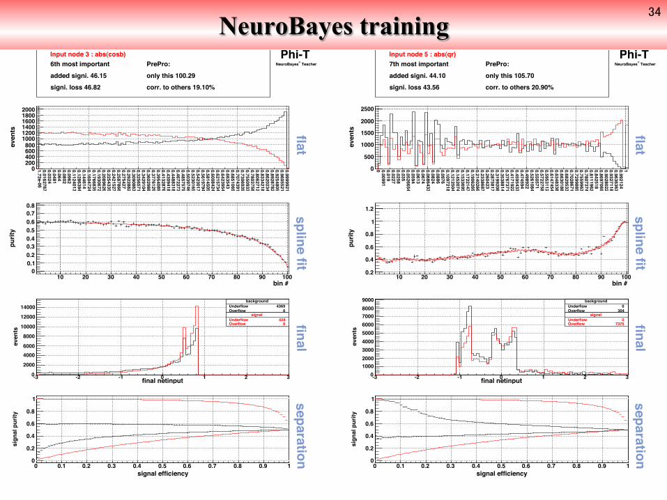
TeacherNeuroBayes
Input node 3 : abs(cosb) PrePro: only this 100.29corr. to others 19.10%
6th most importantadded signi. 46.15signi. loss 46.82
0 0.2 0.4 0.6 0.8 1
even
ts
0200400600800
100012001400160018002000
flat
1.72e-06 0.0162767 0.0324 0.0481 0.064 0.0802 0.0962 0.1124013 0.1286394 0.144614 0.1604724 0.1766835 0.1930672 0.2089626 0.2254335 0.2421527 0.2587866 0.275427 0.2922882 0.3090863 0.3256571 0.3429104 0.3602988 0.3776129 0.3954089 0.4132876 0.4309418 0.4488318 0.4672273 0.4857579 0.5039746 0.5230165 0.5423017 0.5619794 0.5814505 0.6008424 0.6215734 0.6423954 0.663543 0.6851069 0.7074391 0.7306939 0.7550933 0.7803758 0.8062712 0.8334218 0.8620234 0.8928782 0.9254805 0.9605521 0.9999921
bin #10 20 30 40 50 60 70 80 90 100
purit
y
00.10.20.30.40.50.60.70.8 spline fit
final netinput-3 -2 -1 0 1 2 3
even
ts
0
200040006000
800010000
1200014000
backgroundUnderflow 4369Overflow 0
backgroundUnderflow 4369Overflow 0
final netinput-3 -2 -1 0 1 2 3
even
ts
0
200040006000
800010000
1200014000
backgroundUnderflow 4369Overflow 0
signalUnderflow 428Overflow 0
final
signal efficiency0 0.1 0.2 0.3 0.4 0.5 0.6 0.7 0.8 0.9 1
sign
al p
urity
0
0.2
0.4
0.6
0.8
1
separation
signal efficiency0 0.1 0.2 0.3 0.4 0.5 0.6 0.7 0.8 0.9 1
sign
al p
urity
0
0.2
0.4
0.6
0.8
1
separation
Phi-T TeacherNeuroBayes
Input node 5 : abs(qr) PrePro: only this 105.70corr. to others 20.90%
7th most importantadded signi. 44.10signi. loss 43.56
0 0.2 0.4 0.6 0.8 1
even
ts
0
500
1000
1500
2000
2500
flat
0 0.00991 0.019 0.0227 0.0258 0.035 0.0526654 0.0594 0.0613 0.0674 0.0686433 0.0824 0.0886 0.0976 0.1097218 0.1212504 0.1452074 0.1533695 0.1722147 0.1906269 0.2140266 0.2338687 0.260423 0.2875817 0.3199208 0.3538814 0.3767371 0.4171922 0.4595433 0.474594 0.498922 0.5261084 0.550571 0.5722758 0.5953112 0.6147454 0.6348338 0.6630188 0.6829533 0.7028671 0.7299885 0.7559963 0.7807374 0.8111962 0.842518 0.8697069 0.9028022 0.9327118 0.9636363 0.992124 1
bin #10 20 30 40 50 60 70 80 90 100
purit
y
0.2
0.4
0.6
0.8
1
1.2 spline fit
final netinput-3 -2 -1 0 1 2 3
even
ts
0100020003000400050006000700080009000 background
Underflow 0Overflow 304
backgroundUnderflow 0Overflow 304
final netinput-3 -2 -1 0 1 2 3
even
ts
0100020003000400050006000700080009000 background
Underflow 0Overflow 304
signalUnderflow 0Overflow 7375
final
signal efficiency0 0.1 0.2 0.3 0.4 0.5 0.6 0.7 0.8 0.9 1
sign
al p
urity
0
0.2
0.4
0.6
0.8
1
separation
signal efficiency0 0.1 0.2 0.3 0.4 0.5 0.6 0.7 0.8 0.9 1
sign
al p
urity
0
0.2
0.4
0.6
0.8
1
separation34
NeuroBayes training Phi-T
TeacherNeuroBayes
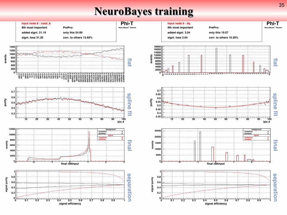
Input node 8 : cosd_b PrePro: only this 54.89corr. to others 13.60%
8th most importantadded signi. 31.19signi. loss 31.20
0 0.2 0.4 0.6 0.8 1
even
ts
0200400600800
100012001400
flat
-1 -0.969 -0.936 -0.9 -0.865 -0.828 -0.79 -0.75 -0.711 -0.671 -0.629 -0.586 -0.541 -0.495 -0.449 -0.401 -0.353 -0.305 -0.257 -0.209 -0.16 -0.112 -0.0631 -0.0133 0.0354793 0.0849 0.1339009 0.1831186 0.228985 0.2761396 0.3204489 0.3642389 0.4080389 0.4514048 0.4934022 0.5331558 0.5734177 0.6102691 0.6468877 0.6820701 0.7162797 0.7504887 0.7828635 0.8134346 0.8431394 0.8717378 0.8996451 0.9265851 0.9519891 0.9768357 0.9999978
bin #10 20 30 40 50 60 70 80 90 100
purit
y
0.3
0.4
0.5
0.6
0.7
spline fitfinal netinput-3 -2 -1 0 1 2 3
even
ts
0
2000
4000
6000
8000
10000
12000 backgroundUnderflow 0Overflow 0
backgroundUnderflow 0Overflow 0
final netinput-3 -2 -1 0 1 2 3
even
ts
0
2000
4000
6000
8000
10000
12000 backgroundUnderflow 0Overflow 0
signalUnderflow 0Overflow 0
final
signal efficiency0 0.1 0.2 0.3 0.4 0.5 0.6 0.7 0.8 0.9 1
sign
al p
urity
0
0.2
0.4
0.6
0.8
1
separation
signal efficiency0 0.1 0.2 0.3 0.4 0.5 0.6 0.7 0.8 0.9 1
sign
al p
urity
0
0.2
0.4
0.6
0.8
1
separation
Phi-T TeacherNeuroBayes
Input node 9 : dq PrePro: only this 19.57corr. to others 10.30%
9th most importantadded signi. 3.04signi. loss 3.04
0 0.2 0.4 0.6 0.8 1
even
ts
02000400060008000
1000012000140001600018000 flat
-29 -7 -5 -5 -4 -4 -3 -3 -3 -3 -2 -2 -2 -2 -2 -2 -1 -1 -1 -1 -1 -1 0 0 0 0 0 0 0 1 1 1 1 1 1 2 2 2 2 2 2 3 3 3 3 4 4 5 5 7 23
bin #10 20 30 40 50 60 70 80 90 100
purit
y
0.350.4
0.450.5
0.550.6
0.650.7 spline fit
final netinput-3 -2 -1 0 1 2 3
even
ts
0
5000
10000
15000
20000
25000 backgroundUnderflow 0Overflow 0
backgroundUnderflow 0Overflow 0
final netinput-3 -2 -1 0 1 2 3
even
ts
0
5000
10000
15000
20000
25000 backgroundUnderflow 0Overflow 0
signalUnderflow 0Overflow 0
final
signal efficiency0 0.1 0.2 0.3 0.4 0.5 0.6 0.7 0.8 0.9 1
sign
al p
urity
0
0.2
0.4
0.6
0.8
1
separation
signal efficiency0 0.1 0.2 0.3 0.4 0.5 0.6 0.7 0.8 0.9 1
sign
al p
urity
0
0.2
0.4
0.6
0.8
1
separation35
NeuroBayes training Phi-T
TeacherNeuroBayes
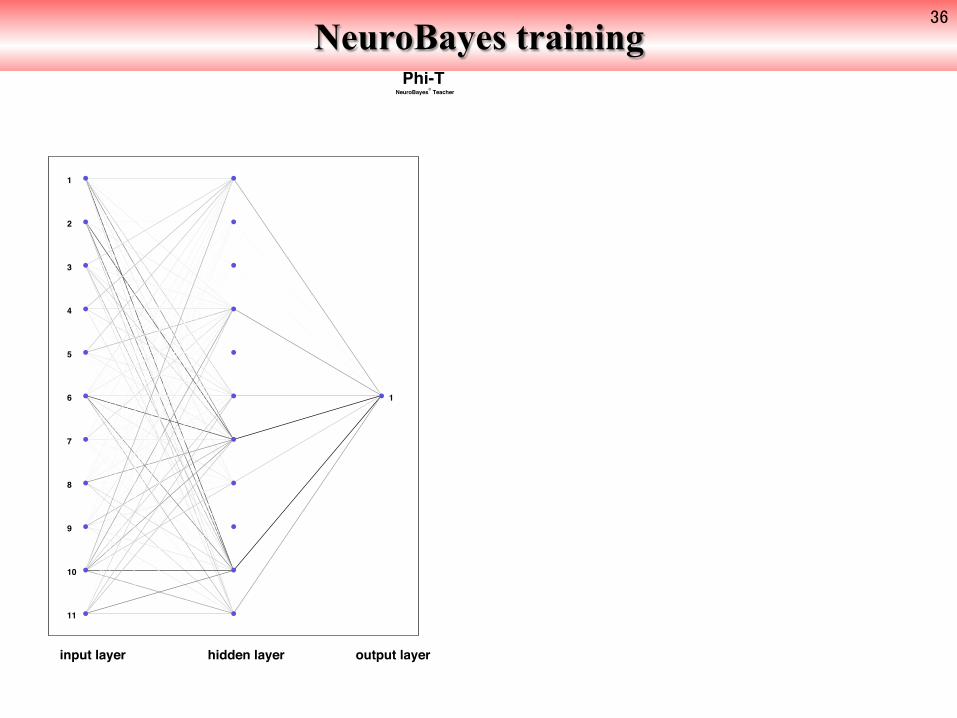
1
2
3
4
5
6
7
8
9
10
11
input layer hidden layer
1
output layer
36
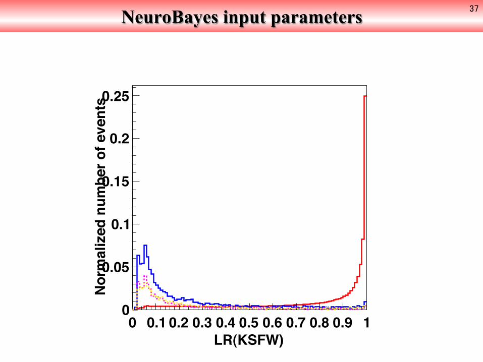
NeuroBayes input parameters 37
LR(KSFW)0 0.1 0.2 0.3 0.4 0.5 0.6 0.7 0.8 0.9 1
Nor
mal
ized
num
ber o
f eve
nts
0
0.05
0.1
0.15
0.2
0.25

NeuroBayes input parameters 38
|B|cos0 0.10.2 0.3 0.40.5 0.6 0.70.8 0.9 1
Probability
0
0.005
0.01
0.015
0.02
0.025
0.03
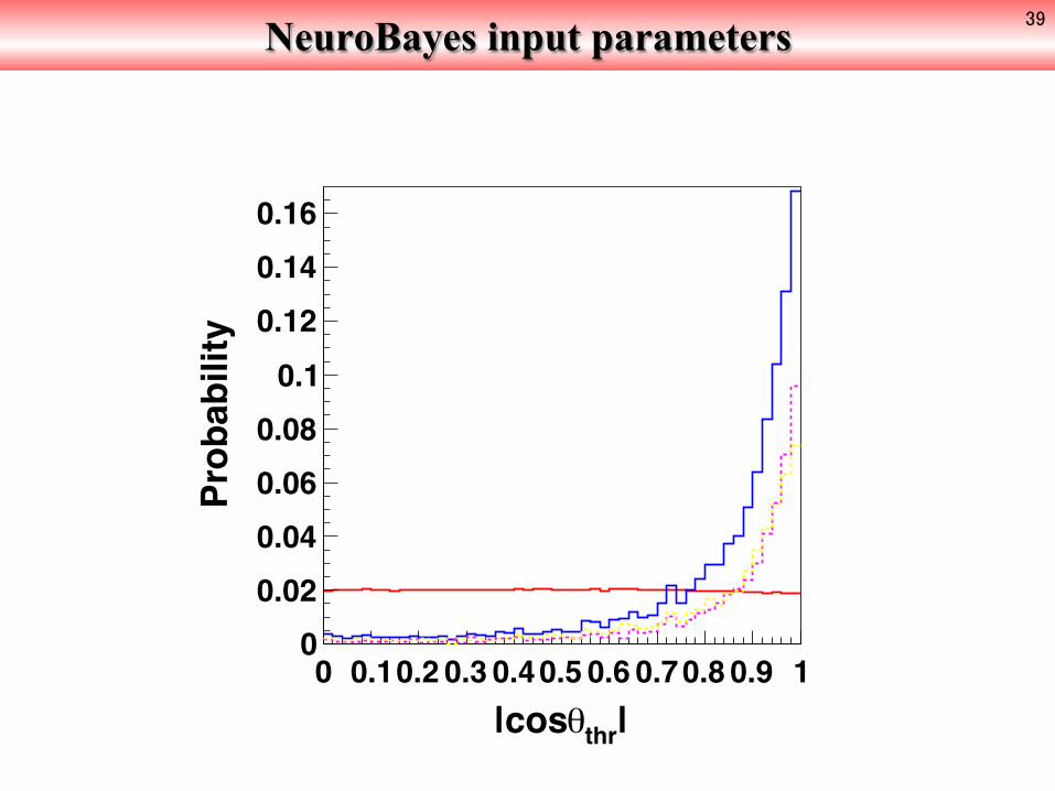
NeuroBayes input parameters 39
|thr|cos0 0.10.2 0.3 0.40.5 0.6 0.70.8 0.9 1
Probability
00.020.040.060.080.10.120.140.16
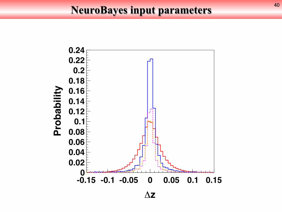
NeuroBayes input parameters 40
z-0.15 -0.1 -0.05 0 0.05 0.1 0.15
Probability
00.020.040.060.080.10.120.140.160.180.20.220.24
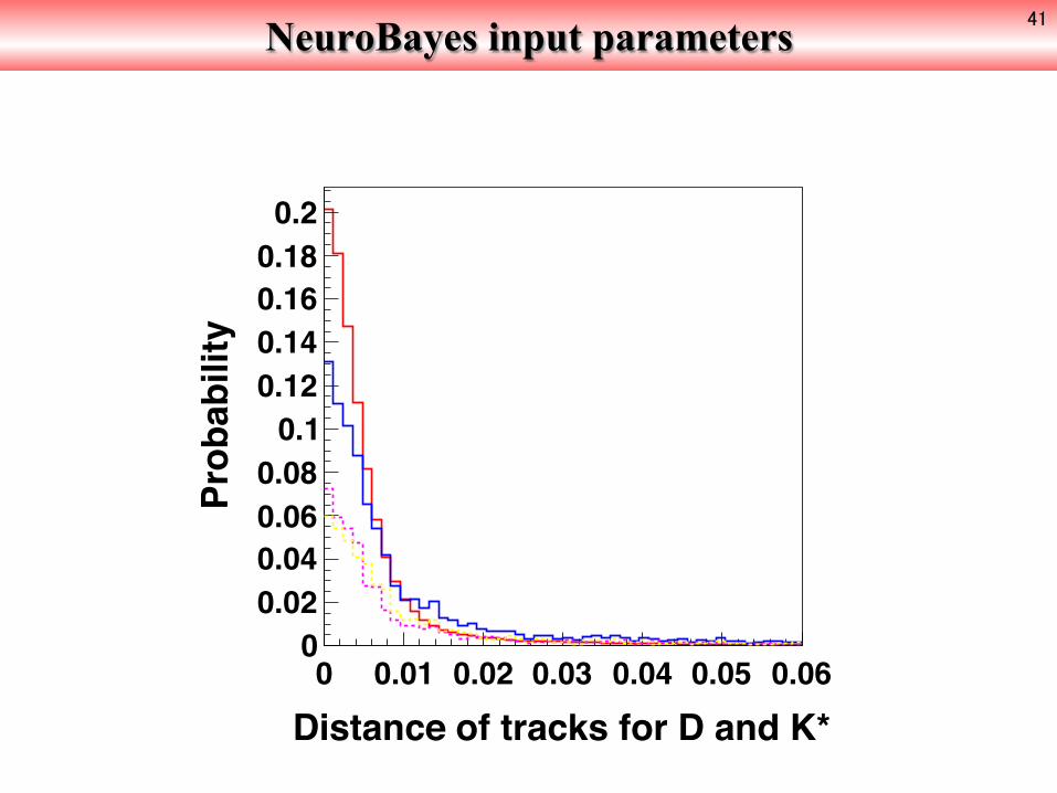
NeuroBayes input parameters 41
Distance of tracks for D and K*0 0.01 0.02 0.03 0.04 0.05 0.06
Prob
abili
ty
00.020.040.060.08
0.10.120.140.160.180.2
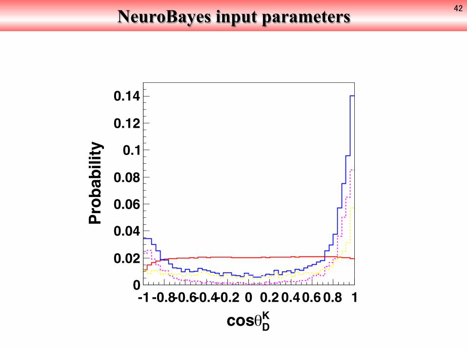
NeuroBayes input parameters 42
DKcos
-1 -0.8-0.6-0.4-0.2 0 0.2 0.40.6 0.8 1
Probability
0
0.02
0.04
0.06
0.08
0.1
0.12
0.14
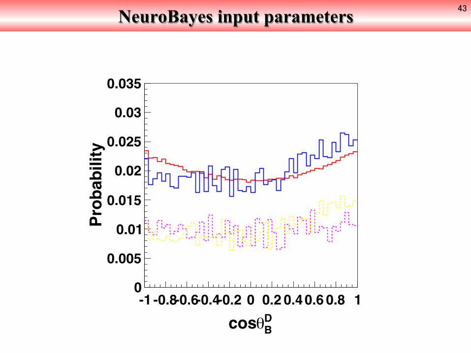
NeuroBayes input parameters 43
BDcos
-1 -0.8-0.6-0.4-0.2 0 0.2 0.40.6 0.8 1
Probability
0
0.005
0.01
0.015
0.02
0.025
0.03
0.035

NeuroBayes input parameters 44
Q-10 -5 0 5 10
Probability
00.020.040.060.080.10.120.140.16
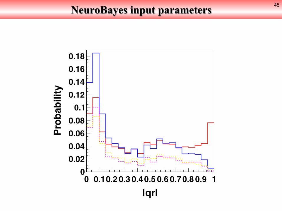
NeuroBayes input parameters 45
|qr|0 0.10.2 0.3 0.40.5 0.6 0.70.8 0.9 1
Probability
00.020.040.060.080.10.120.140.160.18

PDF for ΔE
• Signal: a double Gaussian fixed from signal MC
• Combinatorial BB: free exponential
• D0ρ0 : • D0K+:
• D0π+ :
• Peaking BGs: fixed from MC ‒ [K*0π-]D- K+
• qq: free 1st order Chebychev
PDF for NB’
• Signal: a double Gaussian fixed from signal MC
• Comb. BB:
• D0ρ0: • D0K+: • D0π+: • Peaking BGs:
• qq: a double Gaussian fixed from Mbc sideband of the data.
46
Fixed from MC
Double Gaussians Fixed from MC
We perform ΔE-NB’ 2D fit.
E-0.1-0.05 0 0.05 0.1 0.15 0.2 0.25 0.3
NB
-0.6
-0.4
-0.2
0
0.2
0.4
0.6
0.8
1
E-0.1-0.05 0 0.05 0.1 0.15 0.2 0.25 0.3
NB
-0.6
-0.4
-0.2
0
0.2
0.4
0.6
0.8
1

47
D0K+
E (GeV)-0.1 0 0.1 0.2 0.3
Even
ts /
( 0.0
1 )
0
20
40
60
80
100
120
/ndf = 2.022
E (GeV)-0.1 0 0.1 0.2 0.3
Even
ts /
( 0.0
1 )
0
20
40
60
80
100
120
NBtrans-10 -5 0 5 10
Even
ts /
( 0.5
)
0
50
100
150
200
250
300 0.18± = 1.54 1µ TRANSNB
0.29± = 4.02 2µ TRANSNB
0.057± = 2.180 1 TRANSNB 0.097± = 0.616 1/2 TRANSNB
0.074±/Y = 0.812 1 YTRANSNB 0.27±bb_e = -4.053
33±drho = 352 60±other bb = 1952
/ndf = 0.972
NBtrans-10 -5 0 5 10
Even
ts /
( 0.5
)
0
50
100
150
200
250
300
D0π+ • The yields and shapes are fixed in the fit on signal MC.
Fit for 4 streams of BB MC (no signal).
D0ρ0
Double bifurcated Gauss. Crystal ball

48
E (GeV)-0.1 0 0.1 0.2 0.3
Even
ts /
( 0.0
1 )
020406080
100120140160180
310× 0.000015± = 0.001194 µE 0.000013± = 0.008790 1E
0.056± = 9.079 1/2E 0.00051±/Y = 0.93770 1E Y 0.024± = 1.936
1µ TRANSNB
0.027± = 4.201 2µ TRANSNB
0.0063± = 2.1691 1 TRANSNB 0.0063± = 0.7304 1/2 TRANSNB
0.010±/Y = 0.663 1 YTRANSNB 649±sig = 420961
/ndf = 261.862
E (GeV)-0.1 0 0.1 0.2 0.3
Even
ts /
( 0.0
1 )
020406080
100120140160180
310×
TRANSNB-10 -5 0 5 10
Even
ts /
( 0.4
)0
5000
10000
15000
20000
25000
30000/ndf = 83.002
TRANSNB-10 -5 0 5 10
Even
ts /
( 0.4
)0
5000
10000
15000
20000
25000
30000
E (GeV)-0.1 0 0.1 0.2 0.3
Even
ts /
( 0.0
1 )
0100002000030000400005000060000700008000090000 0.000021± = 0.001190 µE
0.000018± = 0.008776 1E 0.079± = 9.096 1/2E
0.00072±/Y = 0.93786 1E Y 0.038± = 1.903
1µ TRANSNB
0.039± = 4.139 2µ TRANSNB
0.0093± = 2.1769 1 TRANSNB 0.0090± = 0.7393 1/2 TRANSNB
0.016±/Y = 0.644 1 YTRANSNB 458±sig = 209847
/ndf = 124.652
E (GeV)-0.1 0 0.1 0.2 0.3
Even
ts /
( 0.0
1 )
0100002000030000400005000060000700008000090000
TRANSNB-10 -5 0 5 10
Even
ts /
( 0.4
)
0
2000
4000
6000
8000
10000
12000
14000
/ndf = 39.402
TRANSNB-10 -5 0 5 10
Even
ts /
( 0.4
)
0
2000
4000
6000
8000
10000
12000
14000
E (GeV)-0.1 0 0.1 0.2 0.3
Even
ts /
( 0.0
1 )
0
20
40
60
80
100
120
140
/ndf = 6.052
E (GeV)-0.1 0 0.1 0.2 0.3
Even
ts /
( 0.0
1 )
0
20
40
60
80
100
120
140
TRANSNB-10 -5 0 5 10
Even
ts /
( 0.4
)
0
50
100
150
200
250
300 0.033±E_slp = -0.2277
0.041± = -0.7307 1µ TRANSNB
0.12± = 1.74 1 TRANSNB 0.16± = 1.51 1/2 TRANSNB 0.18±/Y = 0.79 1 YTRANSNB
63±bkg = 3240
/ndf = 17.302
TRANSNB-10 -5 0 5 10
Even
ts /
( 0.4
)
0
50
100
150
200
250
300
E (GeV)-0.1 0 0.1 0.2 0.3
Even
ts /
( 0.0
1 )
0
50
100
150
200
250
300
350/ndf = 5.612
E (GeV)-0.1 0 0.1 0.2 0.3
Even
ts /
( 0.0
1 )
0
50
100
150
200
250
300
350
TRANSNB-10 -5 0 5 10
Even
ts /
( 0.4
)
0100200300400500600700800900 0.019±E_slp = -0.0719
0.021± = -0.7787 1µ TRANSNB
0.075± = 1.591 1 TRANSNB 0.054± = 1.514 1/2 TRANSNB
0.11±/Y = 0.69 1 YTRANSNB 104±bkg = 9563
/ndf = 47.702
TRANSNB-10 -5 0 5 10
Even
ts /
( 0.4
)
0100200300400500600700800900
Favored mode Suppressed mode
Signal
qq Mbc sideband
E (GeV)-0.1 0 0.1 0.2 0.3
Even
ts /
( 0.0
1 )
0
20
40
60
80
100
120
/ndf = 2.022
E (GeV)-0.1 0 0.1 0.2 0.3
Even
ts /
( 0.0
1 )
0
20
40
60
80
100
120
NBtrans-10 -5 0 5 10
Even
ts /
( 0.5
)
0
50
100
150
200
250
300 0.18± = 1.54 1µ TRANSNB
0.29± = 4.02 2µ TRANSNB
0.057± = 2.180 1 TRANSNB 0.097± = 0.616 1/2 TRANSNB
0.074±/Y = 0.812 1 YTRANSNB 0.27±bb_e = -4.053
33±drho = 352 60±other bb = 1952
/ndf = 0.972
NBtrans-10 -5 0 5 10
Even
ts /
( 0.5
)
0
50
100
150
200
250
300
E (GeV)-0.1 0 0.1 0.2 0.3
Even
ts /
( 0.0
1 )
0
20
40
60
80
100/ndf = 0.862
E (GeV)-0.1 0 0.1 0.2 0.3
Even
ts /
( 0.0
1 )
0
20
40
60
80
100
NBtrans-10 -5 0 5 10
Even
ts /
( 0.5
)
020406080
100120140160180 0.13± = 1.42
1µ TRANSNB
0.65± = 5.00 2µ TRANSNB
0.068± = 2.206 1 TRANSNB 0.18± = 0.49 1/2 TRANSNB 0.038±/Y = 0.954 1 YTRANSNB
0.23±bb_e = -3.835 24±drho = 112
45±other bb = 1604
/ndf = 0.592
NBtrans-10 -5 0 5 10
Even
ts /
( 0.5
)
020406080
100120140160180
BB MC 4streams
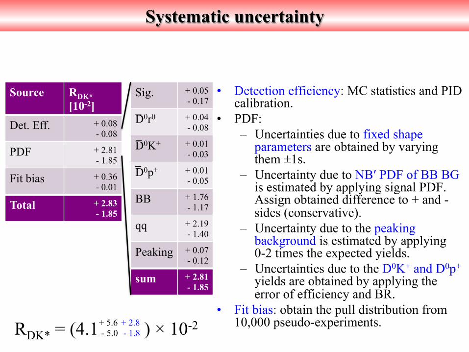
Systematic uncertainty
• Detection efficiency: MC statistics and PID calibration.
• PDF: – Uncertainties due to fixed shape
parameters are obtained by varying them ±1s.
– Uncertainty due to NB′ PDF of BB BG is estimated by applying signal PDF. Assign obtained difference to + and - sides (conservative).
– Uncertainty due to the peaking background is estimated by applying 0-2 times the expected yields.
– Uncertainties due to the D0K+ and D0p+ yields are obtained by applying the error of efficiency and BR.
• Fit bias: obtain the pull distribution from 10,000 pseudo-experiments.
Sig. + 0.05 - 0.17
D0r0 + 0.04 - 0.08
D0K+ + 0.01 - 0.03
D0p+ + 0.01 - 0.05
BB + 1.76 - 1.17
qq + 2.19 - 1.40
Peaking + 0.07 - 0.12
sum + 2.81 - 1.85
Source RDK* [10-2]
Det. Eff. + 0.08 - 0.08
PDF + 2.81 - 1.85
Fit bias + 0.36 - 0.01
Total + 2.83 - 1.85
RDK* = (4.1 ) × 10-2 + 5.6 - 5.0
+ 2.8 - 1.8
_
_
_

Upper limit on RDK*
• We obtain the upper limit by using an asymmetric Gaussian, where the positive and negative widths correspond to positive and negative errors including the syst. err.
RDK* = (4.1 ) × 10-2
< 0.16 (95 % C.L.) BaBar’09 RDK* < 0.24 (95 % C.L.)
asymmetric Gaussian µ = 0.041 upper σ = 0.063 lower σ = 0.054
0.16 (95 % C.L.)
Integrated
50
+ 5.6 - 5.0
+ 2.8 - 1.8