Basics of the modelling of the ground deformations produced

by an earthquake

EO Summer School 2014 Frascati – August 13

Pierre Briole

Content

• Earthquakes and faults • Examples of SAR interferograms of earthquakes • The earthquake cycle • Elastic model • Data needed to constrain the model and the

complementarity of seismological, geodetic and geological data

• Example of models

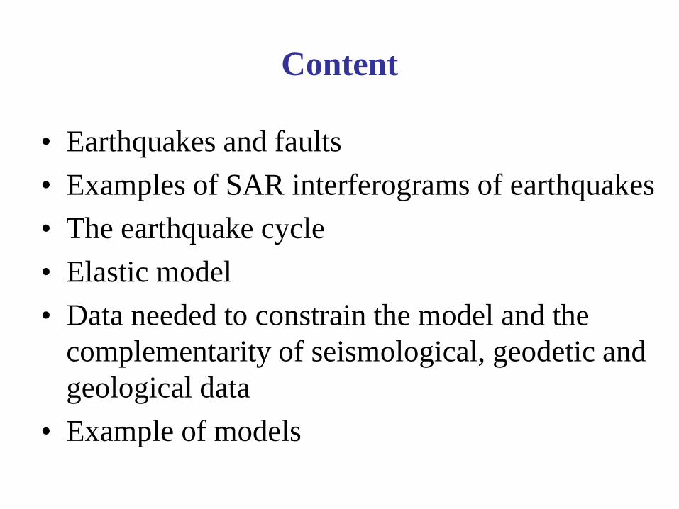
Most earthquakes are located at plates boundaries

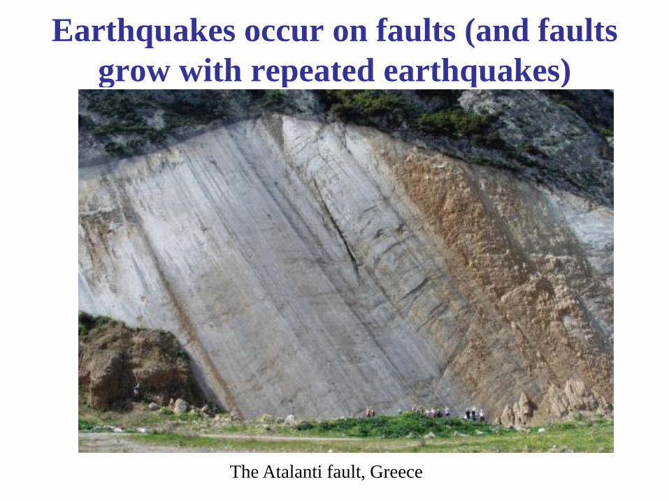
Earthquakes occur on faults (and faults grow with repeated earthquakes)

The Atalanti fault, Greece

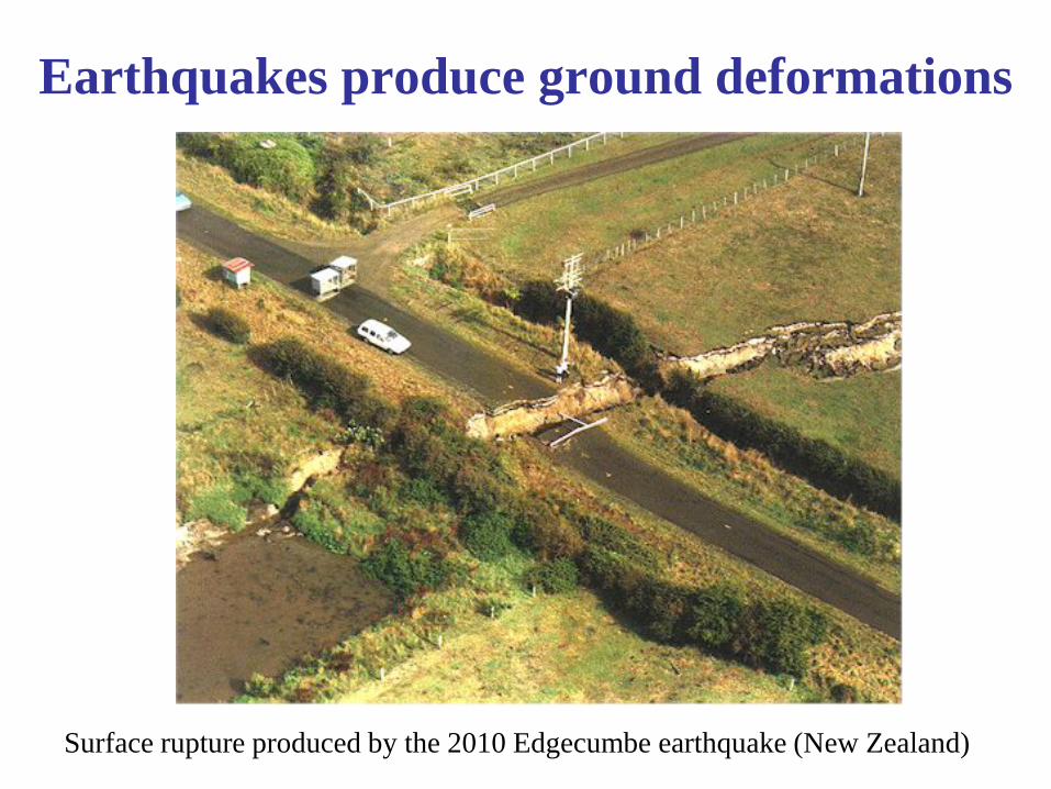
Earthquakes produce ground deformations

Surface rupture produced by the 2010 Edgecumbe earthquake (New Zealand)

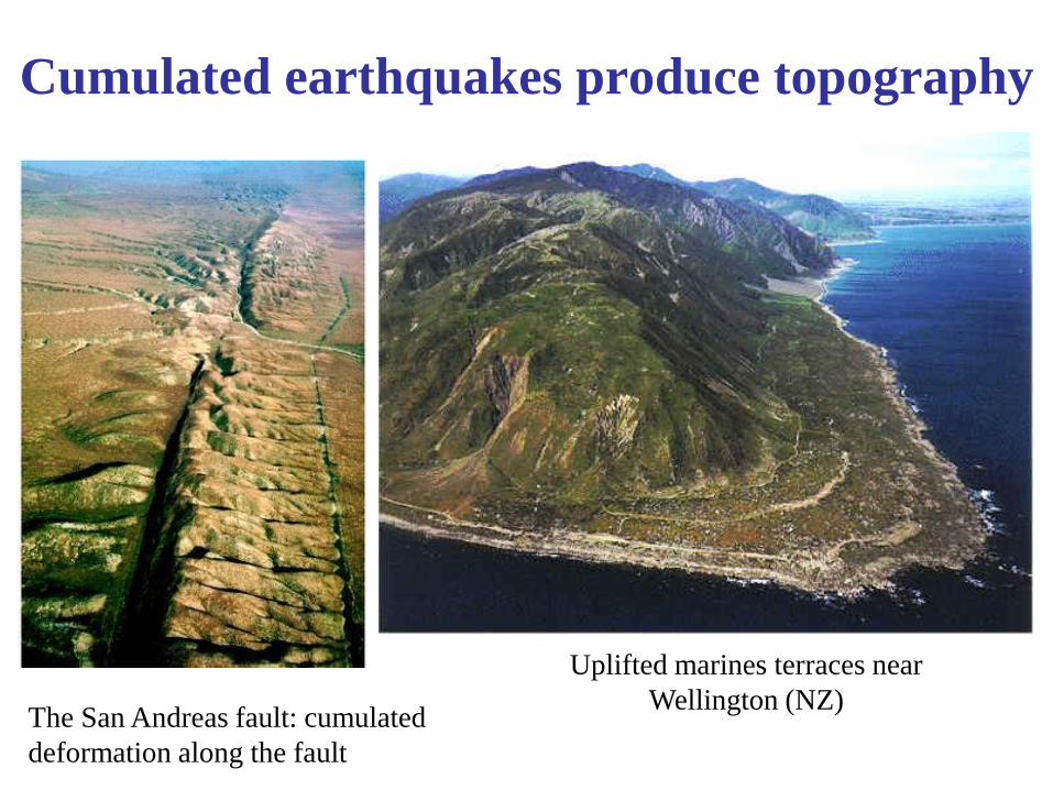
Cumulated earthquakes produce topography

The San Andreas fault: cumulated deformation along the fault

Uplifted marines terraces near Wellington (NZ)

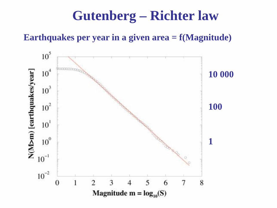
Gutenberg – Richter law Earthquakes per year in a given area = f(Magnitude)

1

100

10 000

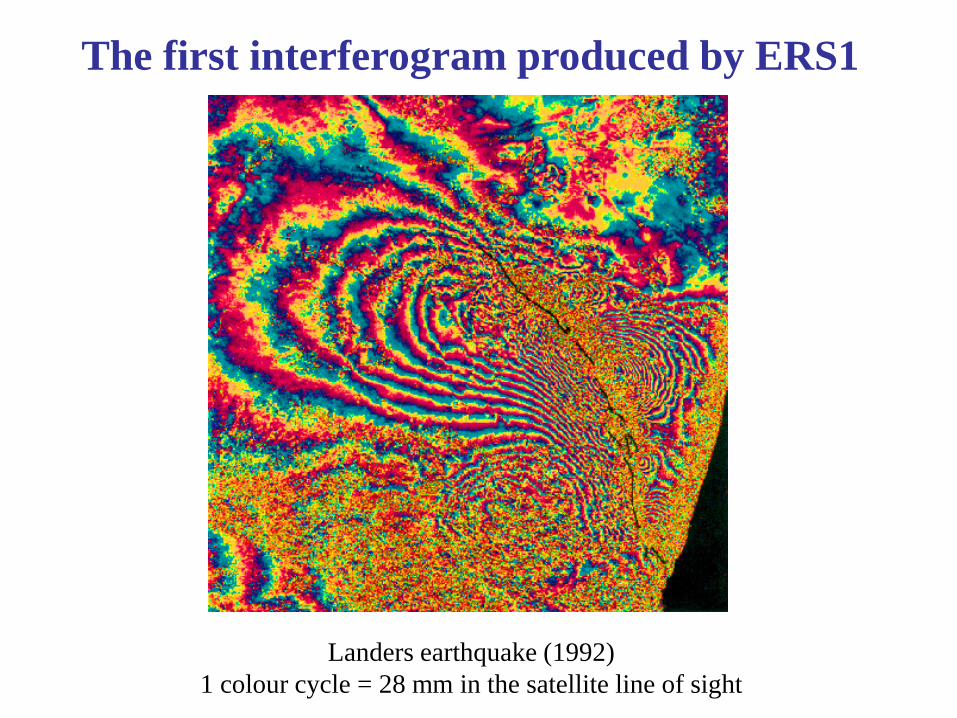
Landers earthquake (1992) 1 colour cycle = 28 mm in the satellite line of sight

The first interferogram produced by ERS1

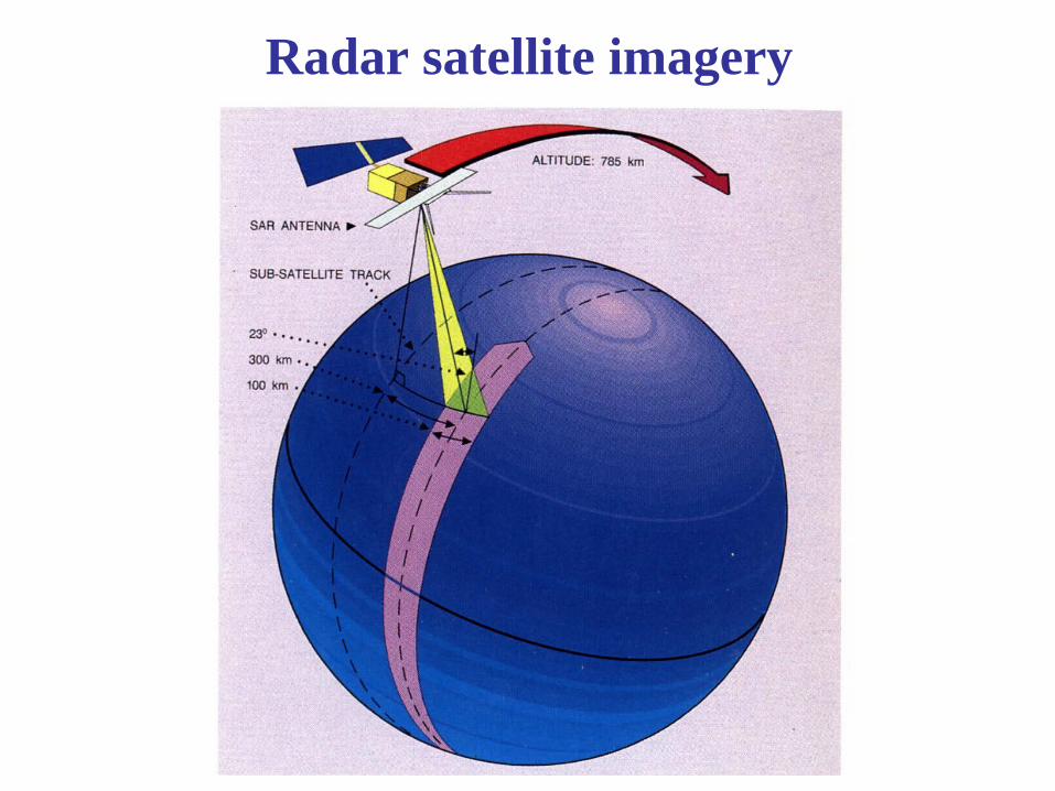
Radar satellite imagery

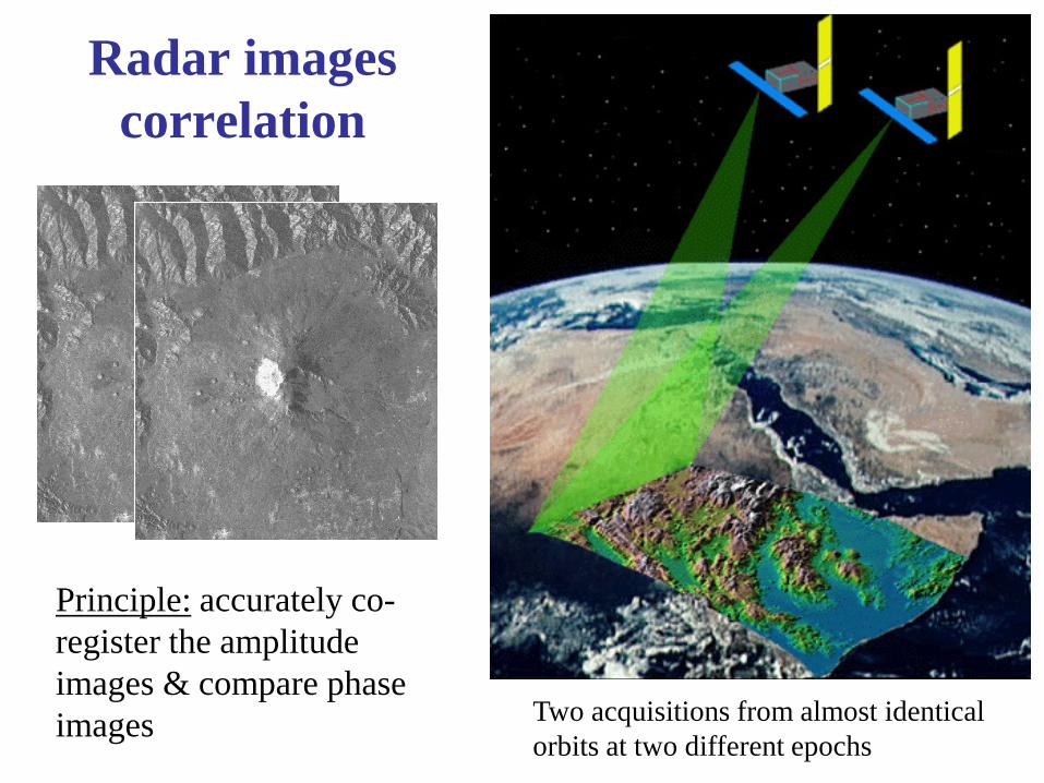
Radar images correlation

Two acquisitions from almost identical orbits at two different epochs

Principle: accurately co-register the amplitude images & compare phase images

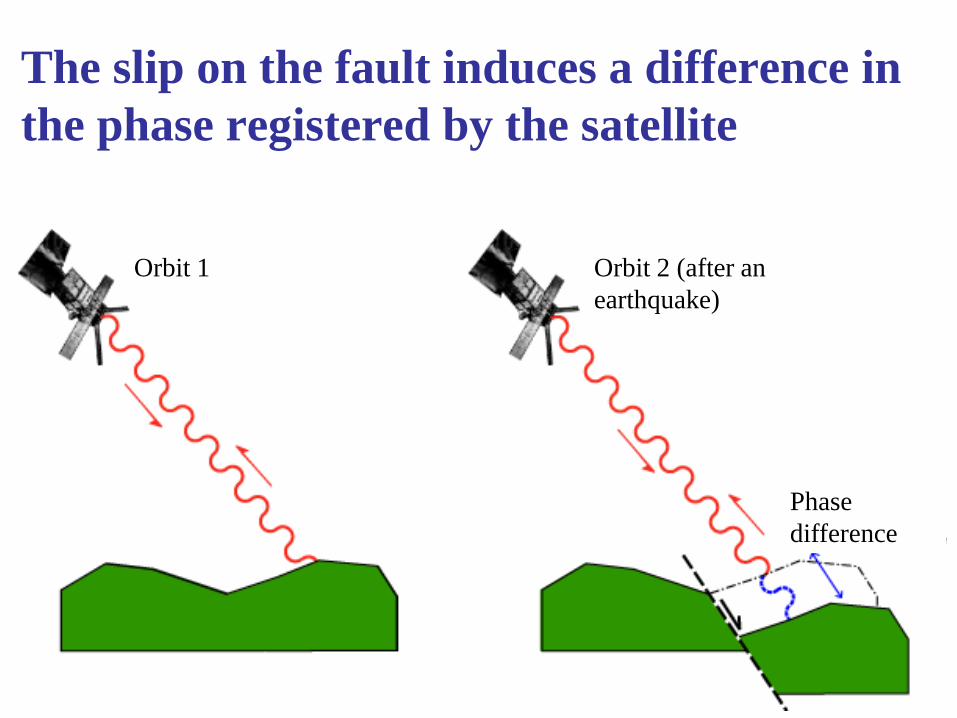
The slip on the fault induces a difference in the phase registered by the satellite

Orbit 1 Orbit 2 (after an earthquake)

Phase difference

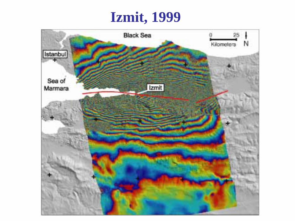
Izmit, 1999

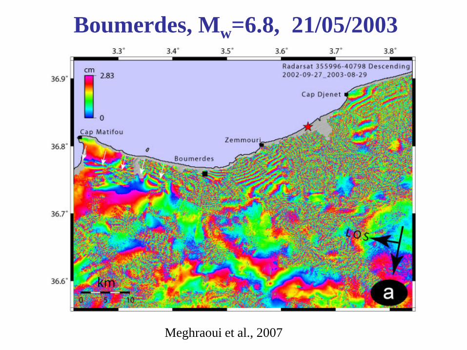
Boumerdes, Mw=6.8, 21/05/2003

Meghraoui et al., 2007

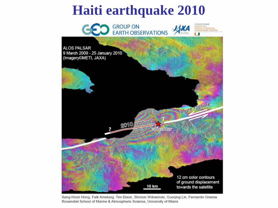
Haiti earthquake 2010

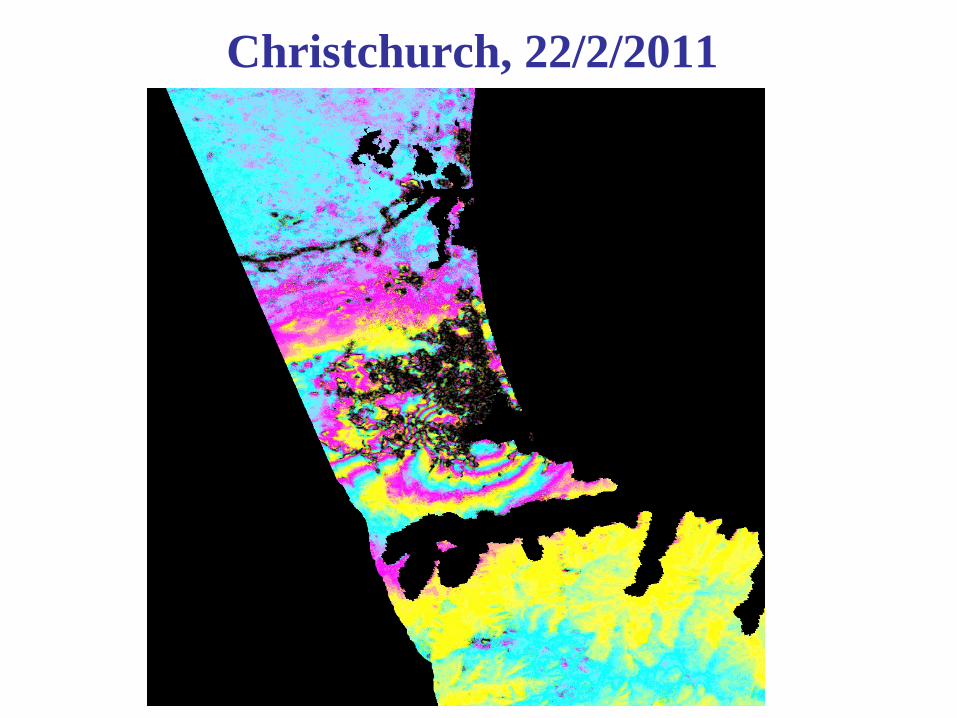
Christchurch, 22/2/2011

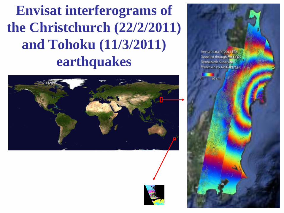
Envisat interferograms of the Christchurch (22/2/2011)

and Tohoku (11/3/2011) earthquakes

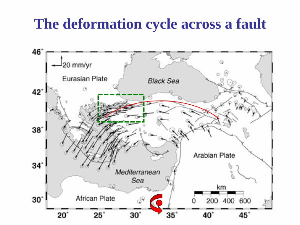
The deformation cycle across a fault

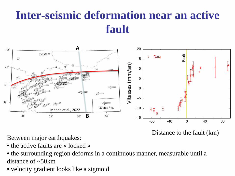
Meade et al., 2022

A

B

Inter-seismic deformation near an active fault

Between major earthquakes: • the active faults are « locked » • the surrounding region deforms in a continuous manner, measurable until a distance of ~50km • velocity gradient looks like a sigmoid

Distance to the fault (km) Vi

tess

es (m

m/a

n)

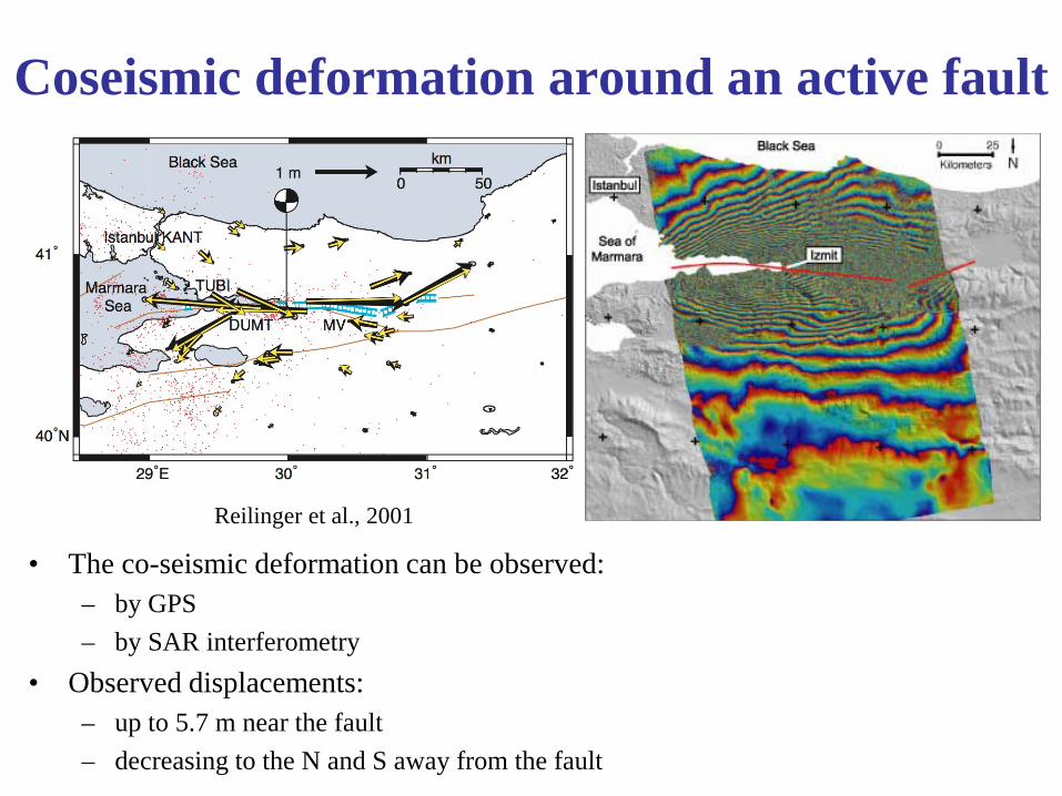
• The co-seismic deformation can be observed: – by GPS – by SAR interferometry

• Observed displacements: – up to 5.7 m near the fault – decreasing to the N and S away from the fault

Reilinger et al., 2001

Coseismic deformation around an active fault

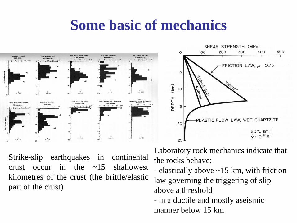
Strike-slip earthquakes in continental crust occur in the ~15 shallowest kilometres of the crust (the brittle/elastic part of the crust)

Laboratory rock mechanics indicate that the rocks behave: - elastically above ~15 km, with friction law governing the triggering of slip above a threshold - in a ductile and mostly aseismic manner below 15 km

Some basic of mechanics

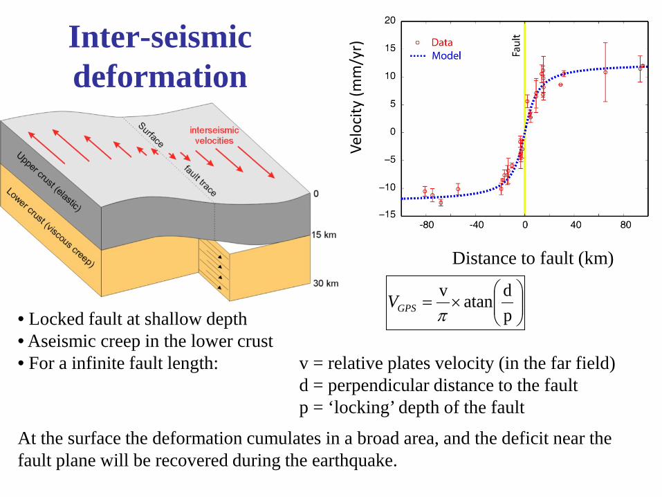
• Locked fault at shallow depth • Aseismic creep in the lower crust • For a infinite fault length: At the surface the deformation cumulates in a broad area, and the deficit near the fault plane will be recovered during the earthquake.

×=

pdatanv

πGPSV

v = relative plates velocity (in the far field) d = perpendicular distance to the fault p = ‘locking’ depth of the fault

Distance to fault (km)

Velo

city

(mm

/yr)

Inter-seismic deformation

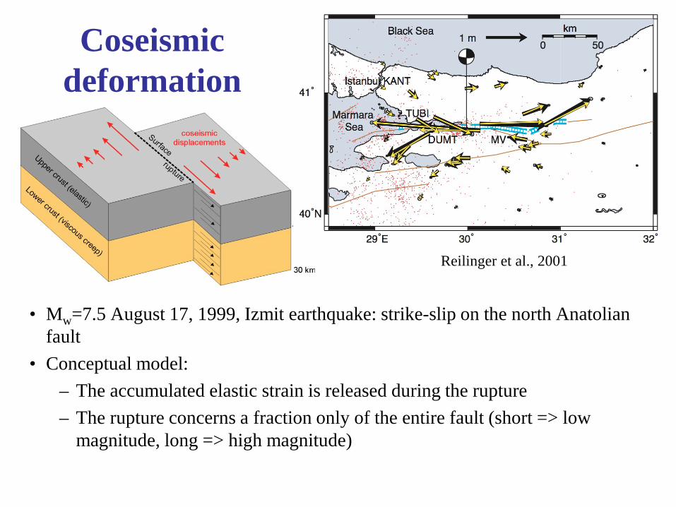
• Mw=7.5 August 17, 1999, Izmit earthquake: strike-slip on the north Anatolian fault

• Conceptual model: – The accumulated elastic strain is released during the rupture – The rupture concerns a fraction only of the entire fault (short => low

magnitude, long => high magnitude)

Reilinger et al., 2001

Coseismic deformation

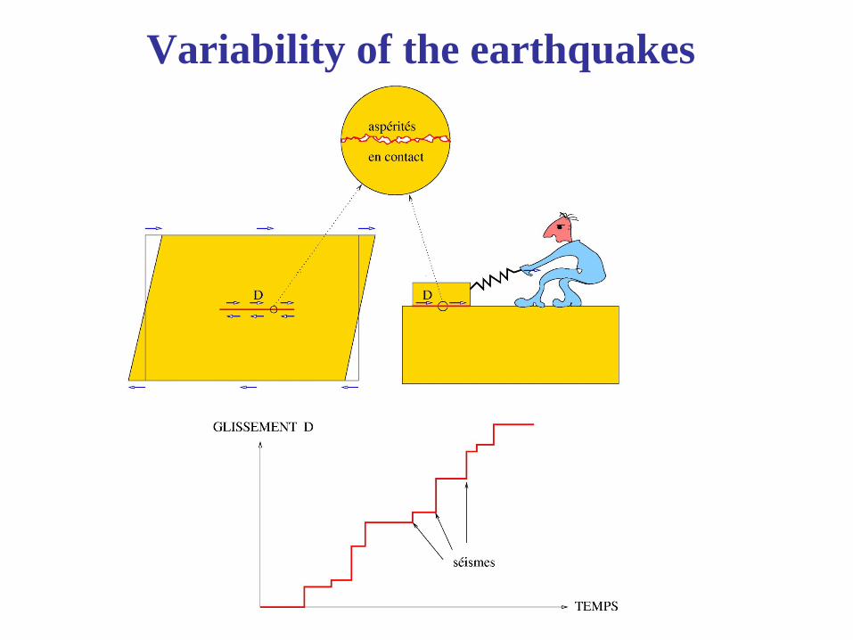
Variability of the earthquakes

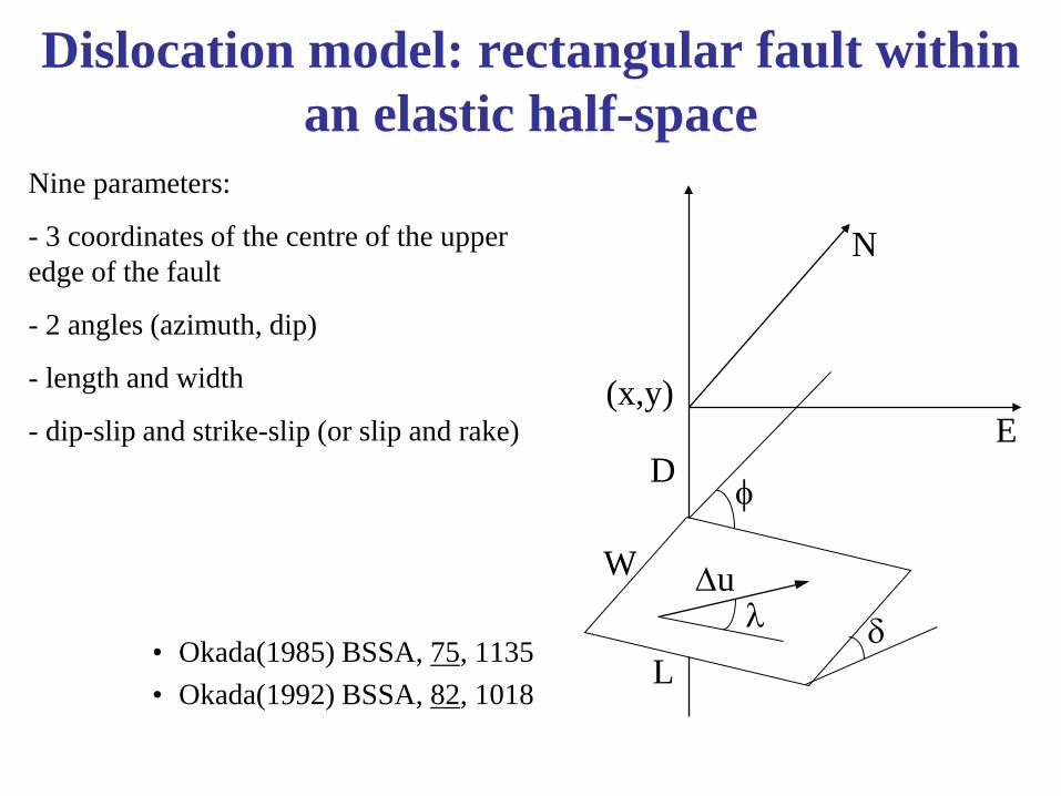
Dislocation model: rectangular fault within an elastic half-space

• Okada(1985) BSSA, 75, 1135 • Okada(1992) BSSA, 82, 1018

δ λ

E

N

φ

L

W

D

(x,y)

∆u

Nine parameters:

- 3 coordinates of the centre of the upper edge of the fault

- 2 angles (azimuth, dip)

- length and width

- dip-slip and strike-slip (or slip and rake)

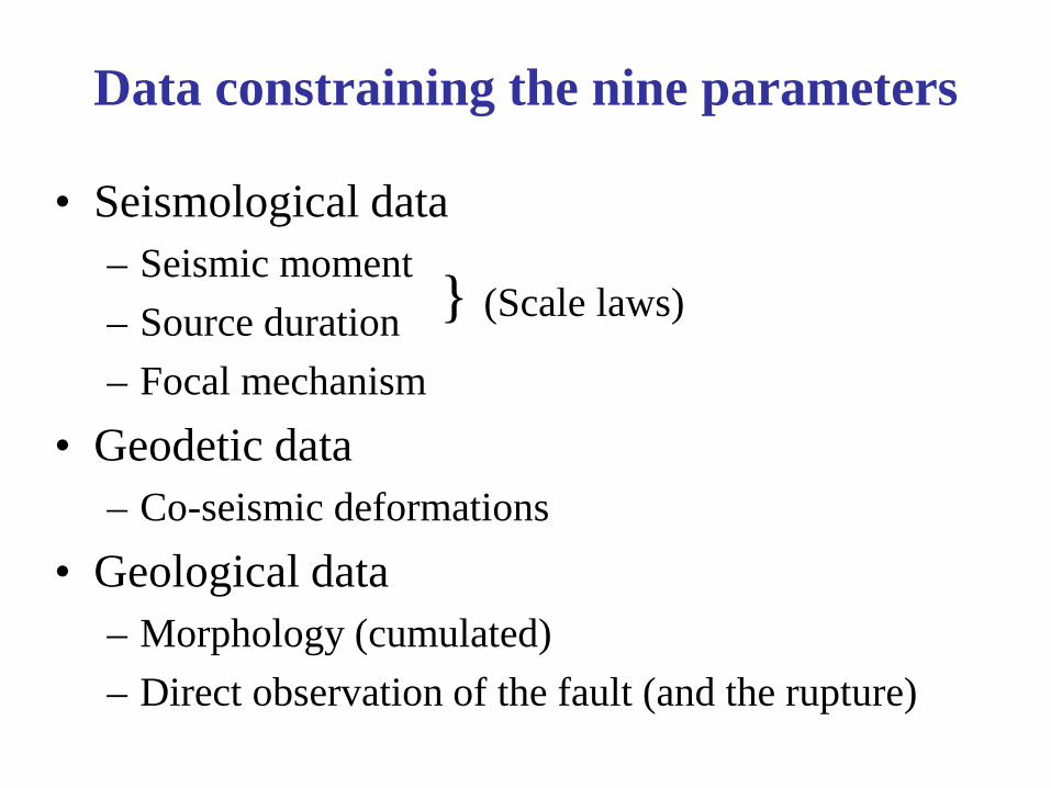
Data constraining the nine parameters

• Seismological data – Seismic moment – Source duration – Focal mechanism

• Geodetic data – Co-seismic deformations

• Geological data – Morphology (cumulated) – Direct observation of the fault (and the rupture)

(Scale laws) }

1. Contraints from seismology

• Seismology constrains relatively well the azimuth and dip angles of the fault (most of the time better than geodesy and geology)

• Seismology constrains well the energy released and therefore the product of the fault surface and slip

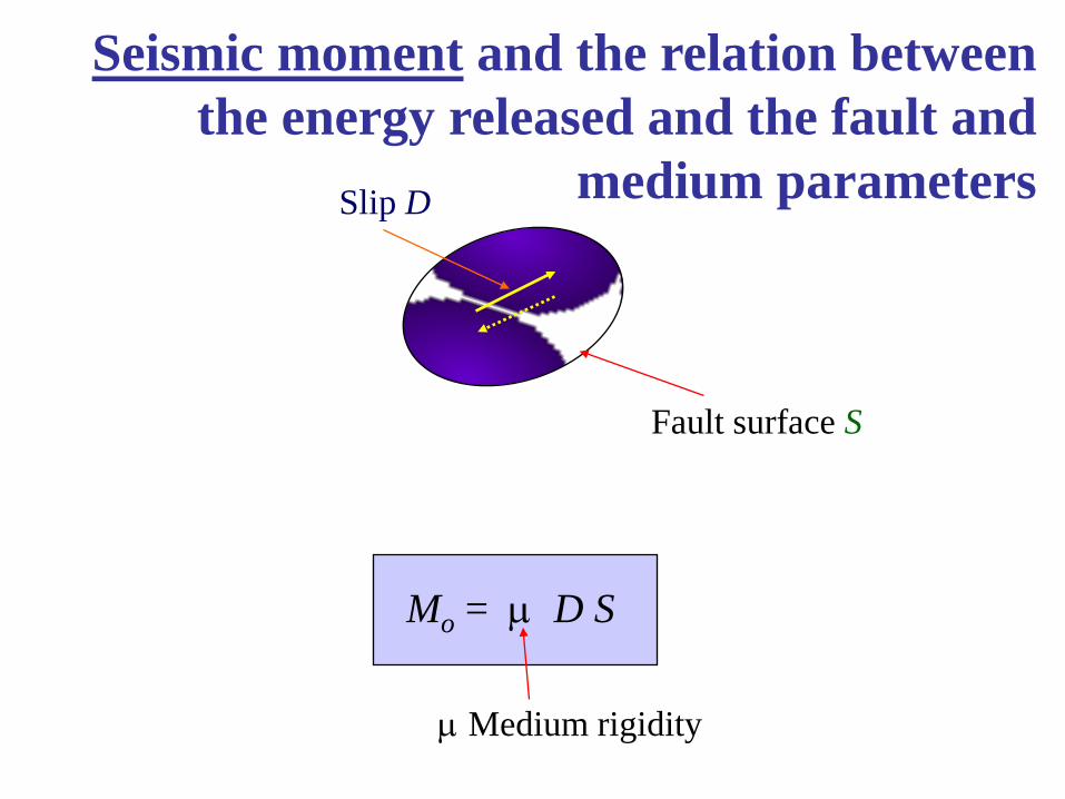
Slip D

Fault surface S

Seismic moment and the relation between the energy released and the fault and

medium parameters

Mo = µ D S

µ Medium rigidity

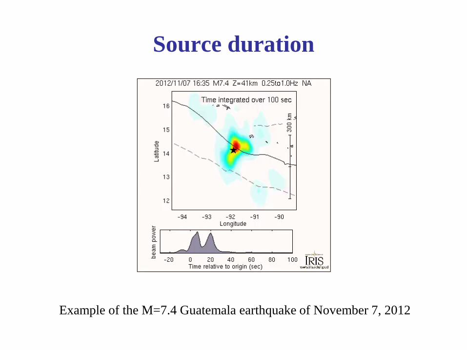
Source duration

Example of the M=7.4 Guatemala earthquake of November 7, 2012

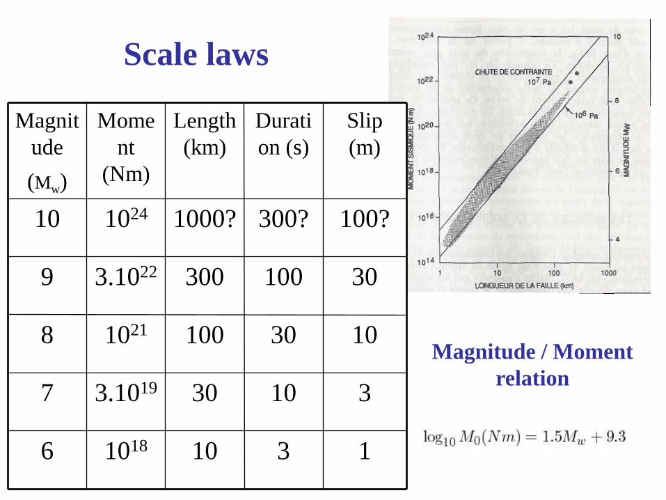
1

3

10

30

100?

Slip (m)

3 10 1018 6

10 30 3.1019 7

30 100 1021 8

100 300 3.1022 9

300? 1000? 1024 10

Duration (s)

Length(km)

Moment

(Nm)

Magnitude (Mw)

Scale laws

Magnitude / Moment relation

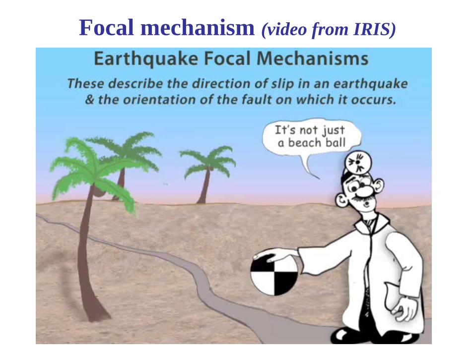
Focal mechanism (video from IRIS)

2. Contraints from geodesy

• Geodesy gives good constraints of the fault location • It gives also good constraints on the fault length and width • It gives good constraints on the slip on fault • It constrains poorly the fault dip angle

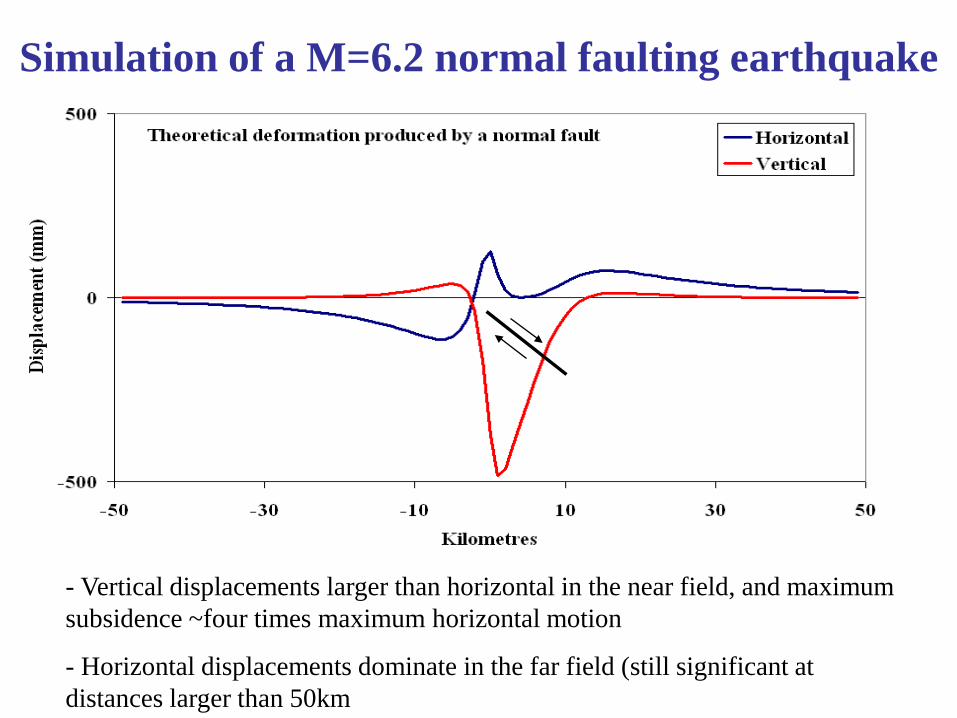
Simulation of a M=6.2 normal faulting earthquake

- Vertical displacements larger than horizontal in the near field, and maximum subsidence ~four times maximum horizontal motion

- Horizontal displacements dominate in the far field (still significant at distances larger than 50km

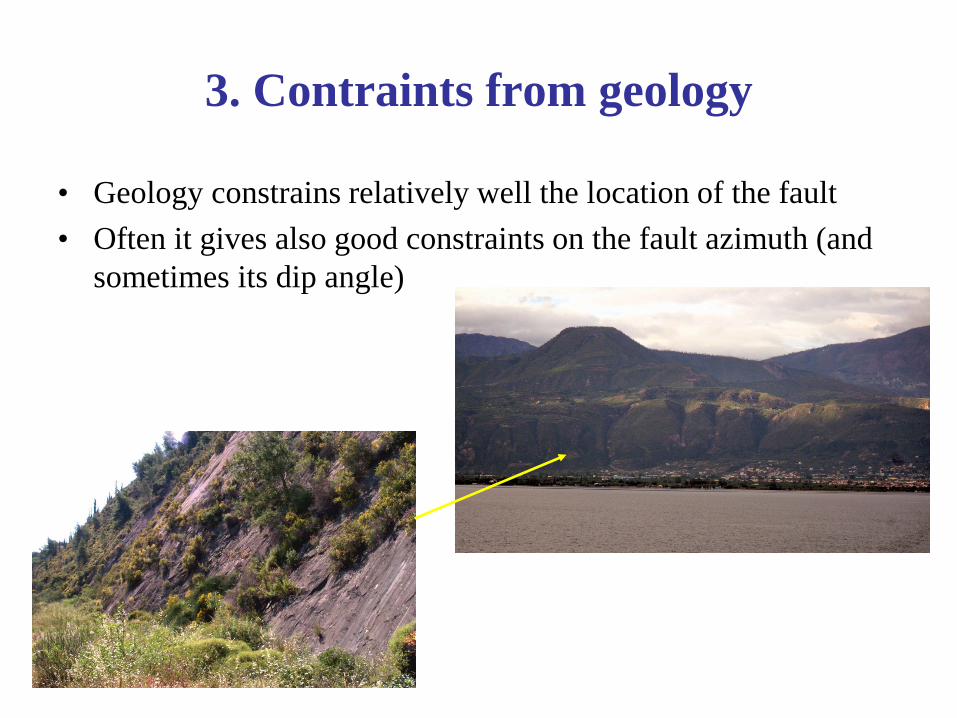
3. Contraints from geology

• Geology constrains relatively well the location of the fault • Often it gives also good constraints on the fault azimuth (and

sometimes its dip angle)

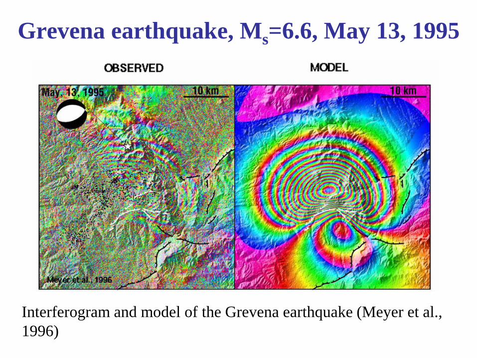
Grevena earthquake, Ms=6.6, May 13, 1995

Interferogram and model of the Grevena earthquake (Meyer et al., 1996)

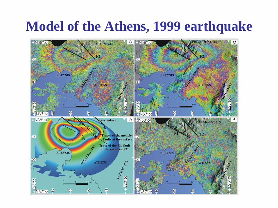
Model of the Athens, 1999 earthquake

Model of the Izmit, 1999 earthquake

Interferogram Synthetic interferogram (assuming a dislocation in an elastic half-space) Residual

interferogram

ESA

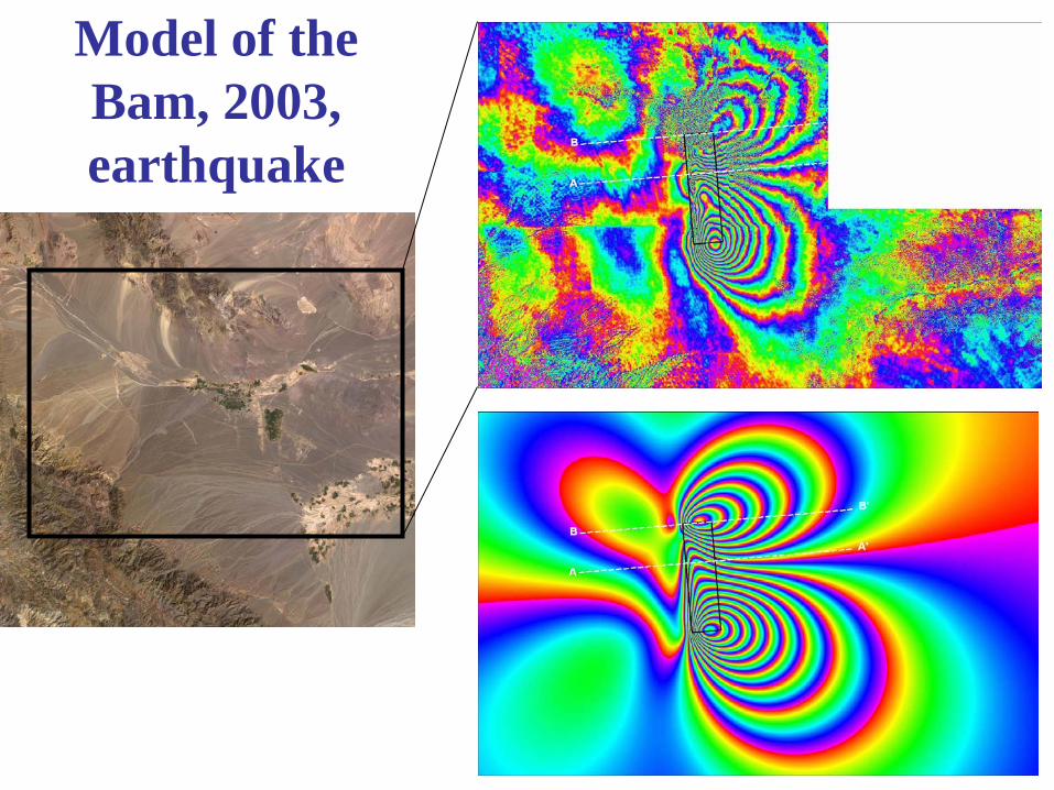
Model of the Bam, 2003, earthquake