Embed Size (px)
DESCRIPTION
Calculation Methods
Citation preview

1
جامعة الملك سعود
قسم اإلحصاء وبحوث العمليات
طرق الحسابات في بحوث العمليات بإستخدام
EXCEL SOLVER, LINGO, AND THE
MATHEMATICAL MODELING
LANGUAGE R
تأليف
د. عدنان ماجد عبد الرحمن بري
استاذ اإلحصاء وبحوث العمليات المشارك

2

3
م هللا الرحمن الرحيمبس
الحمد $ رب العالمين والصالة والسالم على اشرف خلق هللا سيدنا ونبينا محمد وعلى آله وصحبه
وسلم. أما بعد.
EXCEL بإستخدام طرق الحسابات في بحوث العملياتهذه هي المسودة األولى لكتاب SOLVER, LINGO, AND THE MATHEMATICAL MODELING
LANGUAGE R .لطالب مرحلة البكالوريوس " و" النمذجة والمحاكاة –جزء أول –وكما ذكرت في مقدمة كتبي السابقة " طرق التنبؤ اإلحصائي
Excel, SIMAN, Arena and General Purpose Simulation Systemبإستخدام (GPSS WORLD) و بناء النماذج بإستخدام "Excel and Vensim بقيه أن هذا الكتاب كسا
سيظل مسودة إلى ماشاء هللا ألني وبإذن هللا تعالى سوف أقوم بتطويره وتجديده وتحسينه بشكل مستمر وسيظل بشكله اإللكتروني هذا ألني أعتقد ان العلوم والتقنية تتطور يوميا وبشكل متسارع
ثورة بحيث ان وضعها في كتاب جامد ستاتيكي اليتناسب مع ديناميكية الموضوع وخاصة في عصر المعلومات واإلنترنت.
يغطي هذا الكتاب بعض الطرق المستخدمة في الحسابات للمساعدة في حل النماذج التي تنتج عن التكاوين المختلفة لمشاكل األمثلية والتي تغطي البرمجة الرياضية والشبكات والتخصيص والجدولة
وإتخاذ القرار والنمذجة المالية وغيرها.في حل الكثير من األمثلة وذلك لمقدرته الهائلة في حل Excelج صفحات النشر لقد إستخدمت برنام
الصيغ العددية للمشتقات والتكامالت والمعادالت التفاضلية، كما استعرضت مقدرته في إيجاد EXCELالتكامالت بواسطة المحاكاة وتقدير المعالم في النماذج غير خطية. كما استعرضت مقدرة
SOLVER اكل األمثلية في البرمجة الرياضية.في حل مش بقية الكتاب تستعرض بعض الحزم المتخصصة والتي تستخدم لحل مشاكل بحوث العمليات مثل
. Rوبرنامج النمذجة الرياضية LINGOبرنامج النمذجة إلى هذا وارجوا من هللا ان يوفقني في إنجاز هذا العمل لوجهه الكريم وإلثراء المكتبة العربية الفقيرة
مثل هذا الكتاب.سيكون هذا الكتاب مجاني ألي طالب علم وسيكون متواجد على شبكة اإلنترنت في الموقع http://www.abarry.ws/books/CalculationMethodsBookWithR.pdf
وهللا الموفق.
المؤلف د. عدنان ماجد عبد الرحمن بري
جامعة الملك سعود
هـ 1431ربيع الثاني م 2010إبريل
4
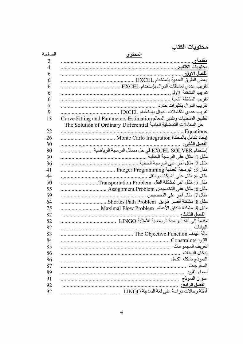
محتويات الكتاب
الصفحة المحتوى 3 ...............................................................................................مقدمة:
4 ...................................................................................ب: محتويات الكتا 6 ........................................................................................الفصل األول:
EXCEL ..................................................... 6بعض الطرق العددية بإستخدام EXCEL ........................................... 6تقريب عددي لمشتقات الدوال بإستخدام
6 تقريب المشتقة األولى .............................................................................. 6 .................................................................تقريب المشتقة الثانية ..............
7 تقريب الدوال بكثيرات حدود ..................................................................... EXCEL .......................................... 9تقريب عددي لتكامالت الدوال بإستخدام
Curve Fitting and Parameters Estimation 13تطبيق المنحنيات وتقدير المعالم The Solution of Ordinary Differentialحل المعادالت التفاضلية العادية
Equations ........................................................................................ 22
Monte Carlo Integration ....................................... 26امل بالمحكاة إيجاد تك 30 ...................................................................................... الفصل الثاني:
30 ....في حل مسائل البرمجة الرياضية ................... EXCEL SOLVERإستخدام 30 : مثال على البرمجة الخطية ..............................................................1مثال 36 : مثال آخر على البرمجة الخطية ........................................................2مثال Integer Programming ....................................... 41: البرمجة العددية 3مثال : مثال على الشبكات والنقل ..............................................................4مثال ........................... Transportation Problem: مثال آخر لمشكلة النقل 5مثال ................................. Assignment Problem: مثال على التخصيص 6مثال : مثال آخر على التخصيص .............................................................7مثال .................................. Shortes Path Problem: مشكلة أقصر طريق 8مثال ............................ Maximal Flow Problem: مشكلة التدفق األعظم 9مثال
44 50 55 59 64 75
82 .................................................................................... الفصل الثالث: LINGO ........................................ 82مقدمة إلى لغة البرمجة الرياضية لألمثلية
82 ...........................................................................................البيانات ... The Objective Function .................................................... 83دالة الهدف
Constraints .............................................................................. 84القيود 85 تعريف المجموعات ............................................................................... 86 إدخال البيانات ......................................................................................
86 لكامل .............................................................................النموذج بشكله ا 87 المخرجات ..........................................................................................
89 .........................................أسماء القيود ................................................ 91 عنوان النموذج .....................................................................................
92 ................................................................................... الفصل الرابع: LINGO ........................................... 92ثلة وحاالت دراسة على لغة النمذجة أم
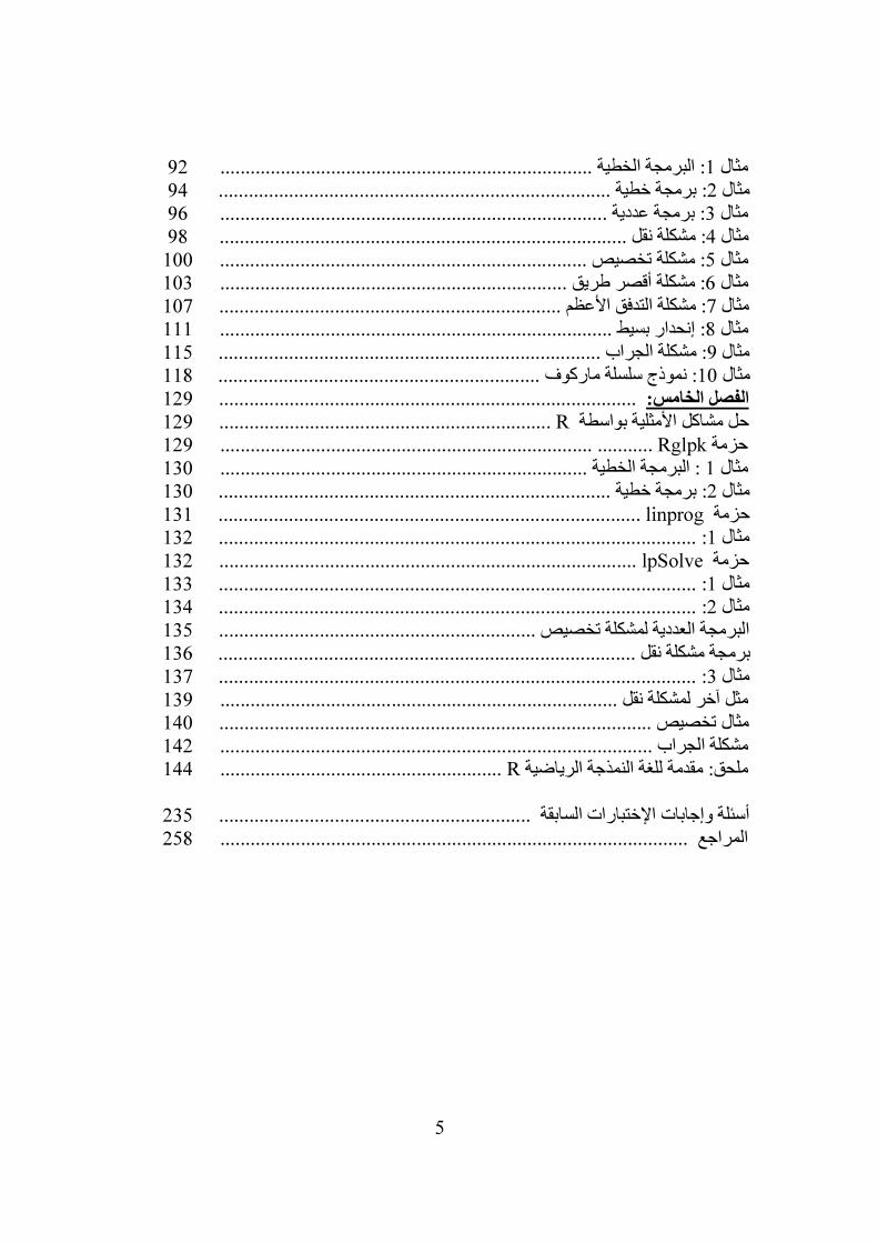
5
: البرمجة الخطية ..........................................................................1مثال .......................: برمجة خطية .......................................................2مثال : برمجة عددية .............................................................................3مثال : مشكلة نقل .................................................................................4مثال ...........................................................: مشكلة تخصيص ..............5مثال : مشكلة أقصر طريق .....................................................................6مثال : مشكلة التدفق األعظم ....................................................................7مثال : إنحدار بسيط ..............................................................................8مثال : مشكلة الجراب ............................................................................9مثال ............................: نموذج سلسلة ماركوف ....................................10مثال
92 94 96 98 100 103 107 111 115 118
129 ................................................................................... الفصل الخامس: R .................................................................. 129حل مشاكل األمثلية بواسطة
........... .......................................................................... Rglpkحزمة : البرمجة الخطية ......................................................................... 1مثال ......................................................: برمجة خطية ........................2مثال
.................................................................................... linprogحزمة .: ..............................................................................................1مثال
................................................................................... lpSolveحزمة : ...............................................................................................1مثال ...................................................: ............................................2مثال
البرمجة العددية لمشكلة تخصيص ...............................................................
برمجة مشكلة نقل ................................................................................... ............................................................................................: ...3مثال
مثل آخر لمشكلة نقل ............................................................................... .................................مثال تخصيص .....................................................
مشكلة الجراب ...................................................................................... ........................................................ Rملحق: مقدمة للغة النمذجة الرياضية
129 130 130 131 132 132 133 134 135 136 137 139 140 142 144
235 أسئلة وإجابات اإلختبارات السابقة ..............................................................
258 المراجع .............................................................................................
6
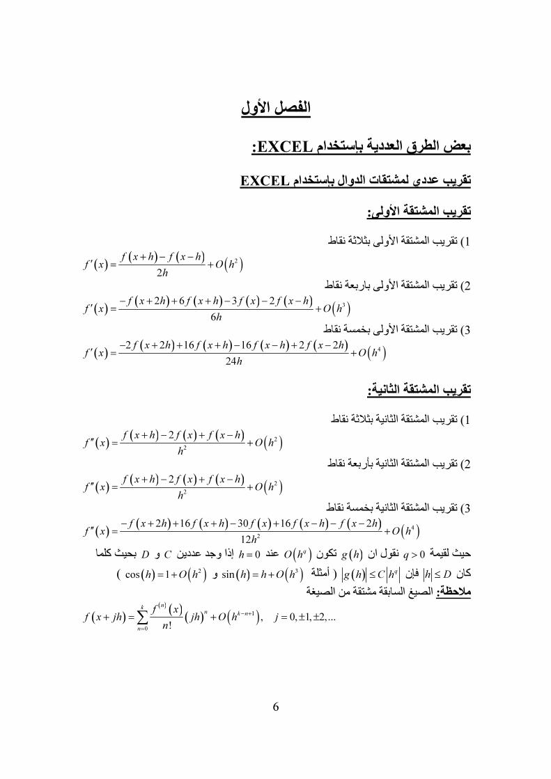
ألولالفصل ا
:EXCELبعض الطرق العددية بإستخدام
EXCELتقريب عددي لمشتقات الدوال بإستخدام
تقريب المشتقة األولى:
) تقريب المشتقة األولى بثالثة نقاط1
( )( ) ( )
( )22
f x h f x hf x O h
h
+ − −′ = +
) تقريب المشتقة األولى باربعة نقاط2
( )( ) ( ) ( ) ( )
( )32 6 3 2
6
f x h f x h f x f x hf x O h
h
− + + + − − −′ = +
لى بخمسة نقاط) تقريب المشتقة األو3
( )( ) ( ) ( ) ( )
( )42 2 16 16 2 2
24
f x h f x h f x h f x hf x O h
h
− + + + − − + −′ = +
تقريب المشتقة الثانية:
) تقريب المشتقة الثانية بثالثة نقاط1
( )( ) ( ) ( )
( )22
2f x h f x f x hf x O h
h
+ − + −′′ = +
) تقريب المشتقة الثانية بأربعة نقاط2
( )( ) ( ) ( )
( )22
2f x h f x f x hf x O h
h
+ − + −′′ = +
) تقريب المشتقة الثانية بخمسة نقاط3
( )( ) ( ) ( ) ( ) ( )
( )42
2 16 30 16 2
12
f x h f x h f x f x h f x hf x O h
h
− + + + − + − − −′′ = +
0qحيث لقيمة )نقول ان < )g h تكون( )qO h 0عندh بحيث كلما Dو Cإذا وجد عددين =
hكان D≤ فإن( ) qg h C h≤ أمثلة )( ) ( )3sin h h O h= )و + ) ( )2cos 1h O h= + (
الصيغ السابقة مشتقة من الصيغة مالحظة:
( )( ) ( )
( ) ( )10
, 0, 1, 2,...!
nk
n k n
n
f xf x jh jh O h j
n
− +
=
+ = + = ± ±∑
7
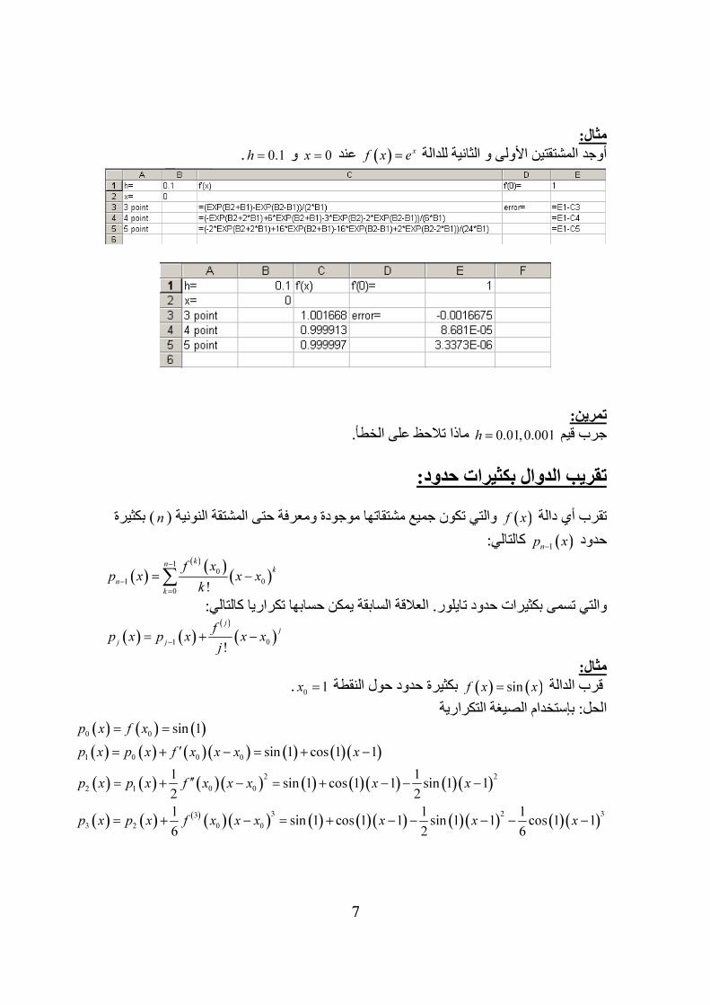
مثال:
)أوجد المشتقتين األولى و الثانية للدالة ) xf x e= 0عندx 0.1hو = =.
تمرين:0.01,0.001hجرب قيم ماذا تالحظ على الخطأ. =
تقريب الدوال بكثيرات حدود:
)تقرب أي دالة )f x موجودة ومعرفة حتى المشتقة النونية (والتي تكون جميع مشتقاتهاn بكثيرة (
)حدود )1np x
−
كالتالي:
( )( ) ( )
( )1
0
1 0
0 !
kn
k
n
k
f xp x x x
k
−
−
=
= −∑
والتي تسمى بكثيرات حدود تايلور. العالقة السابقة يمكن حسابها تكراريا كالتالي:
( ) ( )( )
( )1 0
!
jj
j j
fp x p x x x
j−
= + −
مثال:
)الدالة قرب ) ( )sinf x x= بكثيرة حدود حول النقطة0
1x =. الحل: بإستخدام الصيغة التكرارية
( ) ( ) ( )
( ) ( ) ( ) ( ) ( ) ( )( )
( ) ( ) ( ) ( ) ( ) ( )( ) ( )( )
( ) ( ) ( ) ( ) ( ) ( ) ( )( ) ( )( ) ( )( )
0 0
1 0 0 0
2 2
2 1 0 0
3 2 33
3 2 0 0
sin 1
sin 1 cos 1 1
1 1sin 1 cos 1 1 sin 1 1
2 2
1 1 1sin 1 cos 1 1 sin 1 1 cos 1 1
6 2 6
p x f x
p x p x f x x x x
p x p x f x x x x x
p x p x f x x x x x x
= =
′= + − = + −
′′= + − = + − − −
= + − = + − − − − −

8
تمرين:
)قرب الدالة ) xf x e= حول النقطة0
0x =.

9
EXCELت الدوال بإستخدام تقريب عددي لتكامال
)سوف نقوم بإجراء تكامالت عددية من الشكل )b
a
f x dx∫ الفترة ،[ ],a b 1تقسم إلىN فترات <
عند النقاط 0 1, ,...,
Na x x x b= =.
0hسوف نرمز لحجم الخطوة بالرمز ويكون <1k k
x x h+= ونرمز للدالة عند +
kx بالرمز
( )k kf f x= وζ .هي نقطة في مجال التكامل
) قاعدة الترابزويد البسيطة:1
( ) ( ) ( )1
0
3
0 1,
2 12
x
x
h hf x dx f f error f ζ′′≈ + = −∫
البسيطة:) قاعدة سمبسون 2
( ) ( ) ( ) ( )2
0
5
4
0 1 24 ,
3 90
x
x
h hf x dx f f f error f ζ≈ + + = −∫
3) قاعدة سمبسون 3
8
( ) ( ) ( ) ( )3
0
5
4
0 1 2 3
3 33 3 ,
8 80
x
x
h hf x dx f f f f error f ζ≈ + + + = −∫
) قاعدة بود البسيطة:4
( ) ( ) ( ) ( )4
0
7
6
0 2 3 4
2 87 32 32 7 ,
45 945
x
x
h hf x dx f f f f error f ζ≈ + + + = −∫
قواعد مركبة:
سوف نرمز لحجم الخطوة بالرمز 1i i
b ah x x
N+
−
= − و =1k k
x x h+= )و + )k k
f f x= وζ هي
نقطة في مجال التكامل. ) قاعدة الترابزويد المركبة:1
( )( )
( )2
0
1 1,
2 2 12
bN
Na
b a hf ff x dx h f f error f ζ
−
− ′′≈ + + + + = −
∫ ⋯
) قاعدة الترابزويد المعدلة:2
( ) ( )
( ) ( ) ( )
0
1 1 1 1 1 1
4
4
,2 2 24
11
720
bN
N N Na
f f hf x dx h f f f f f f
b a herror f ζ
− − − +
≈ + + + + + − + + −
−= −
∫ ⋯
) قاعدة سمبسون المركبة:3
( ) ( ) ( )
( ) ( ) ( )
0 1 3 2 2 4 1
4
4
4 2 ,3
, , 2180
b
M M Ma
hf x dx f f f f f f f f
b a h b aerror f h M N
Mζ
− −
≈ + + + + + + + + +
− − = − = =
∫ ⋯ ⋯
10
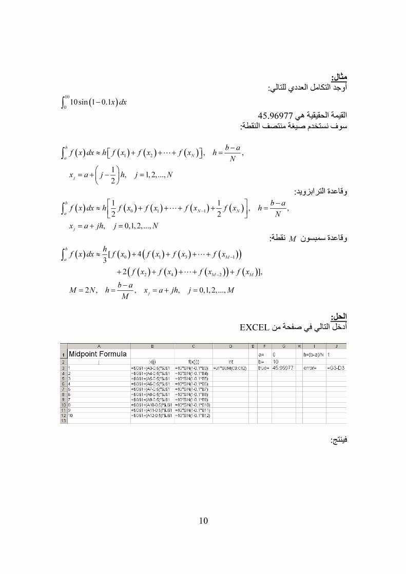
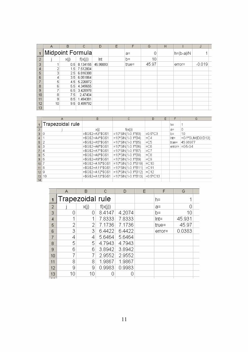
ثال:م أوجد التكامل العددي للتالي:
( )10
0
10sin 1 0.1x dx−∫
45.96977القيمة الحقيقية هي سوف نستخدم صيغة منتصف النقطة:
( ) ( ) ( ) ( )1 2, ,
1, 1, 2,...,
2
b
Na
j
b af x dx h f x f x f x h
N
x a j h j N
−≈ + + + =
= + − =
∫ ⋯
وقاعدة الترابزويد:
( ) ( ) ( ) ( ) ( )0 1 1
1 1, ,
2 2
, 0,1, 2,...,
b
N Na
j
b af x dx h f x f x f x f x h
N
x a jh j N
−
− ≈ + + + + =
= + =
∫ ⋯
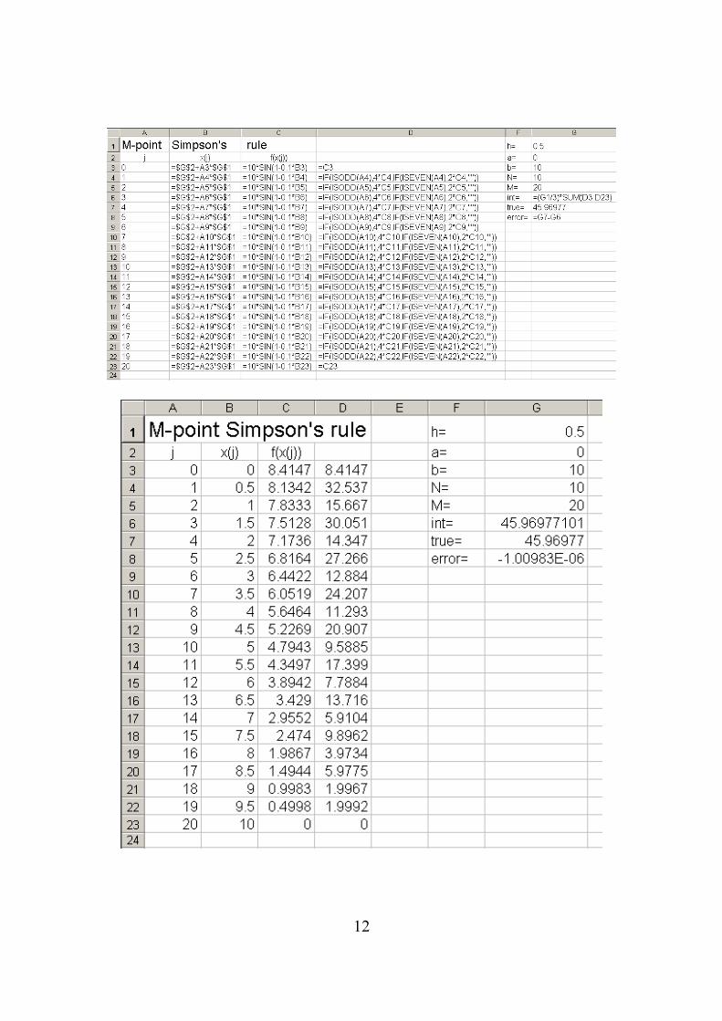
نقطة: Mوقاعدة سمبسون
( ) ( ) ( ) ( ) ( )( )
( ) ( ) ( )( ) ( )
0 1 3 1
2 4 2
[ 43
2 ],
2 , , , 0,1,2,...,
b
Ma
M M
j
hf x dx f x f x f x f x
f x f x f x f x
b aM N h x a jh j M
M
−
−
≈ + + + +
+ + + + +
−= = = + =
∫ ⋯
⋯
الحل:
EXCELأدخل التالي في صفحة من
فينتج:
11
12
13
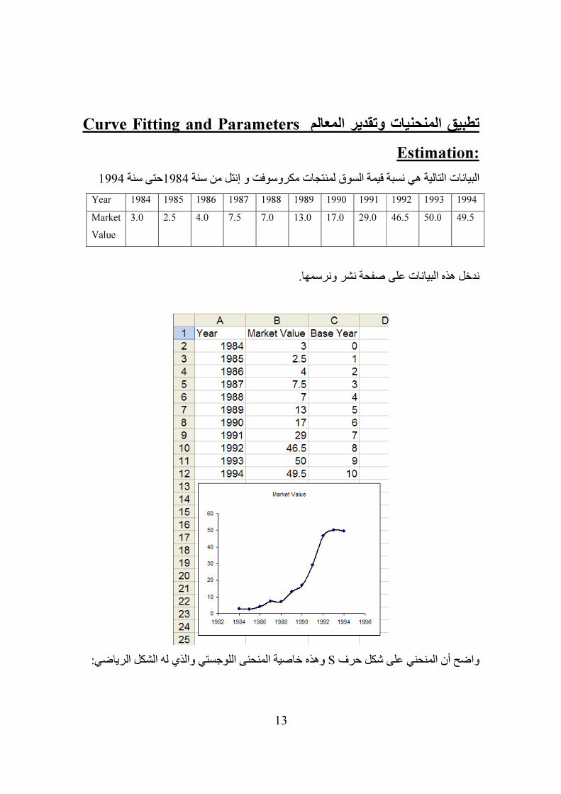
Curve Fitting and Parametersتطبيق المنحنيات وتقدير المعالم
ion:Estimat
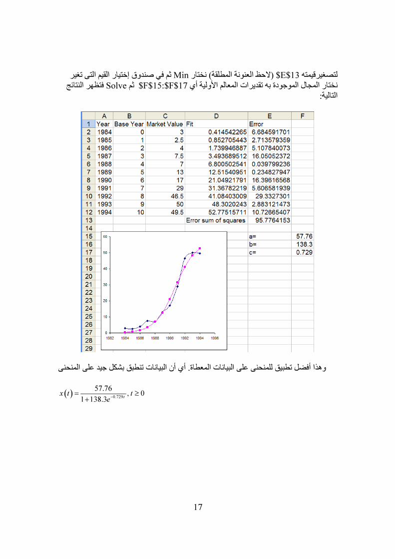
1994حتى سنة 1984البيانات التالية هي نسبة قيمة السوق لمنتجات مكروسوفت و إنتل من سنة
1994 1993 1992 1991 1990 1989 1988 1987 1986 1985 1984 Year
49.5 50.0 46.5 29.0 17.0 13.0 7.0 7.5 4.0 2.5 3.0 Market
Value
.ندخل هذه البيانات على صفحة نشر ونرسمها
وهذه خاصية المنحنى اللوجستي والذي له الشكل الرياضي: Sواضح أن المنحني على شكل حرف
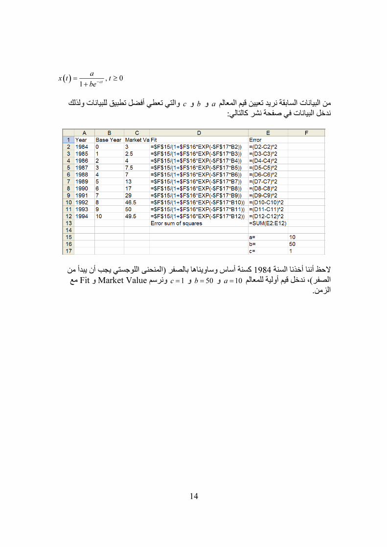
14
( ) , 01
ct
ax t t
be−
= ≥
+
ي أفضل تطبيق للبيانات ولذلك والتي تعط cو bو aمن البيانات السابقة نريد تعيين قيم المعالم
ندخل البيانات في صفحة نشر كالتالي:
كسنة أساس وساويناها بالصفر (المنحنى اللوجستي يجب أن يبدأ من 1984الحظ أننا أخذنا السنة 10aالصفر)، ندخل قيم أولية للمعالم 50bو = 1cو = مع Fitو Market Valueونرسم =
الزمن.

15
الحظ أن المنحنى للقيم المطبقة بعيد عن المنحنى الناتج من البيانات لهذا نجرب قيم مختلفة للمعالم كالتالي:

16
40aمن الشكلين السابقين نجد أن القيم األولية للمعالم 100bو = 1cو = مناسبة، نضع المؤشر = من قائمة األدوات كالتالي: Solverونختار E13في الخلية المراد تصغيرقيمتها
فتظهر النافذة التالية:
17
ر ثم في صندوق إختيار القيم التى تغي Min(الحظ العنونة المطلقة) نختار E$13$لتصغيرقيمته فتظهر النتائج Solveثم F$15:$F$17$نختار المجال الموجودة به تقديرات المعالم األولية أي
التالية:
وهذا أفضل تطبيق للمنحنى على البيانات المعطاة. أي أن البيانات تنطبق بشكل جيد على المنحنى
( )0.729
57.76, 0
1 138.3t
x t t
e−
= ≥
+

18
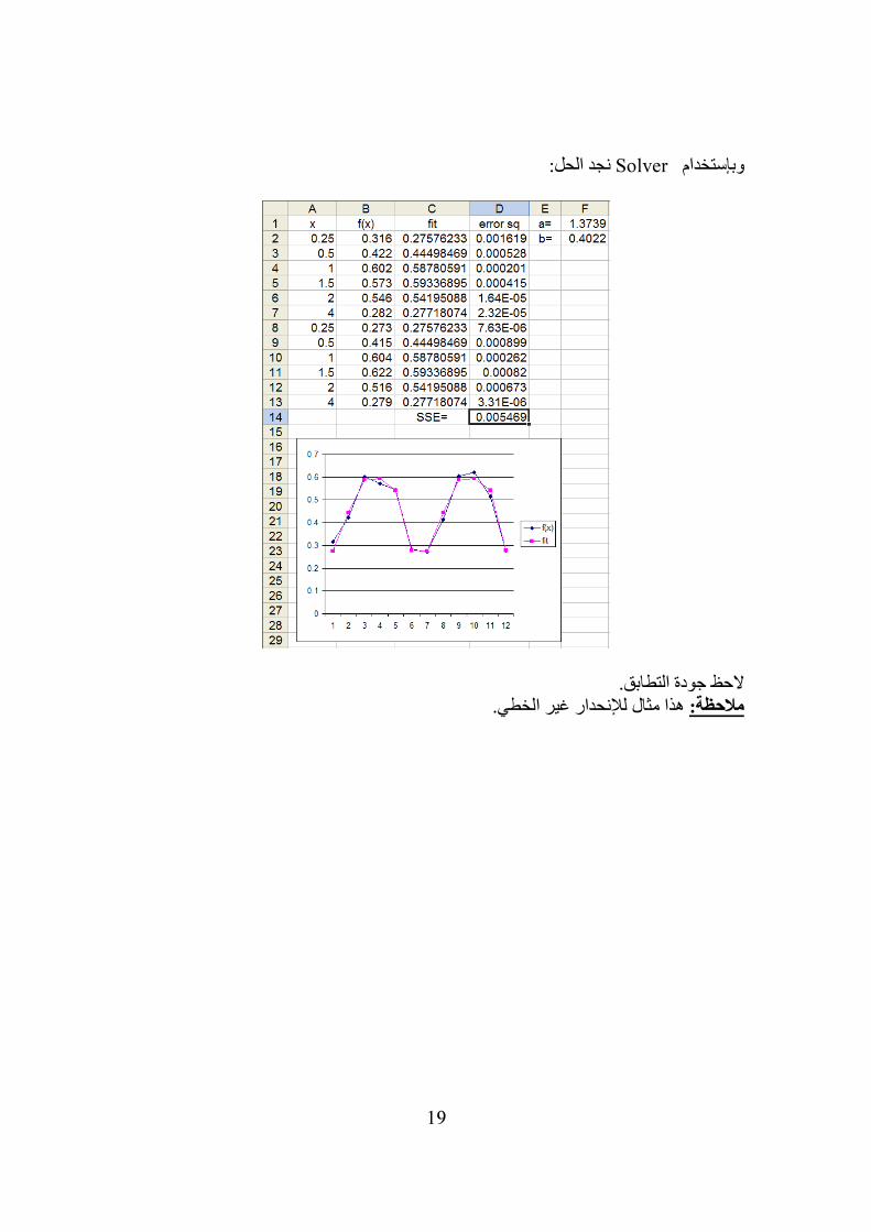
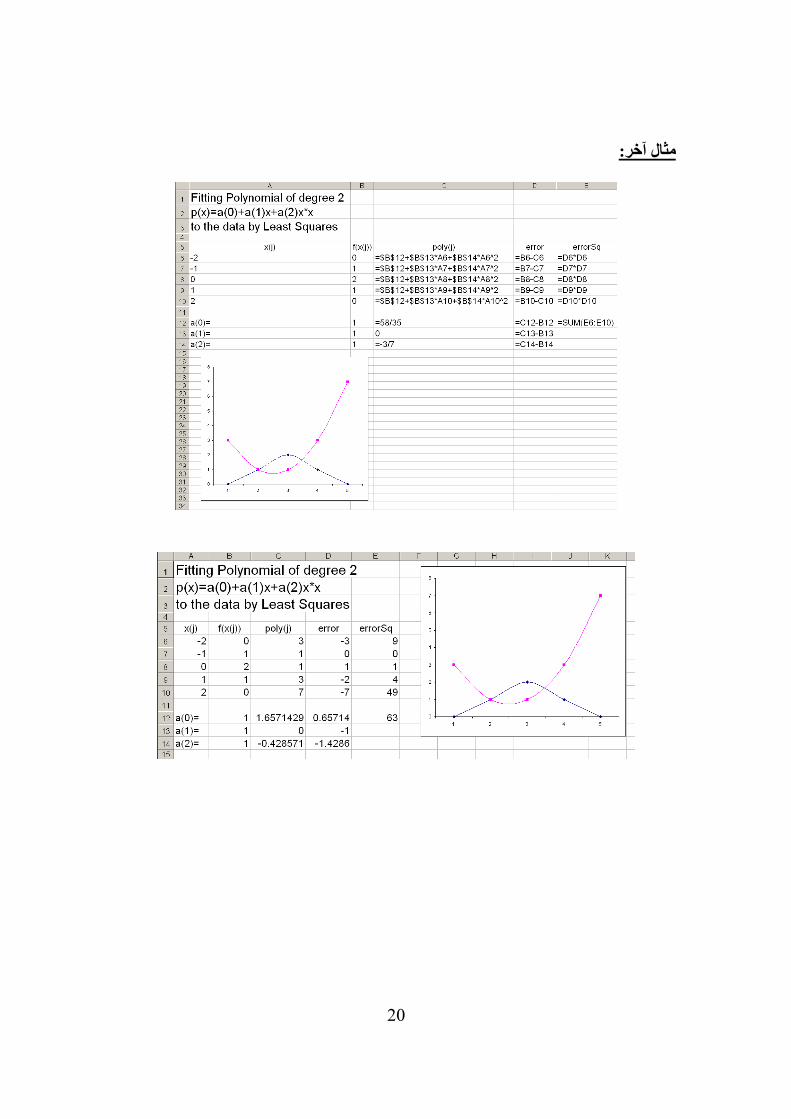
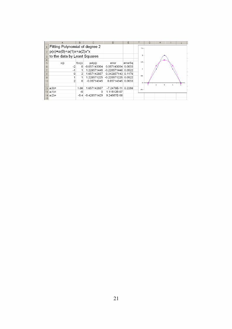
مثال آخر:
البيانات هذه الدالة سوف نطبق على
( )( )bx axa e e
f xa b
− −
−
=
−
19
نجد الحل: Solver وبإستخدام
الحظ جودة التطابق. مالحظة: هذا مثال لإلنحدار غير الخطي.
20
مثال آخر:
21

22
e Solution of Ordinary Differential Thحل المعادالت التفاضلية العادية:
Equations
حل المعادلة التفاضلية العادية التي على الشكل:
( ) ( )( ) ( )0 0, ,y x f x y x y x y′ = =
وسوف نوجد الحل في الفترة المحدودة Initial Value Problemوتسمى بمشكلة القيمة األولية [ ]0
,x b ة مبتدئين بالقيمة األولي0x سوف نكتب( )j j
y y x= .للسهولة
Euler’s Formula) صيغة أويلر 1
( )1
2 1
1 2
,
,2 2
j j
j j
j j
k f x y
h hk f x y k
y y h k+
=
= + +
= +
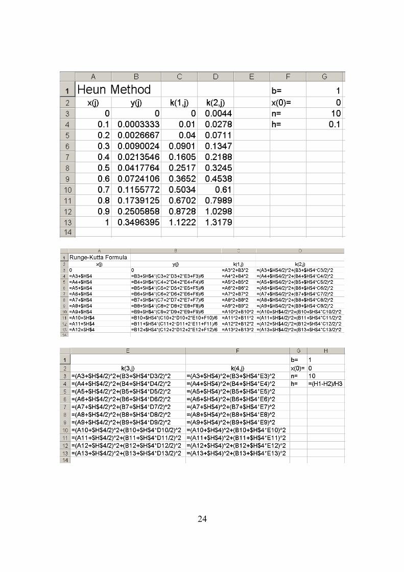
Heun Method) طريقة هيون 2( )1
2 1
1 1 2
,
2 2,
3 3
1 3
4 4
j j
j j
j j
k f x y
k f x h y hk
y y h k k+
=
= + +
= + +
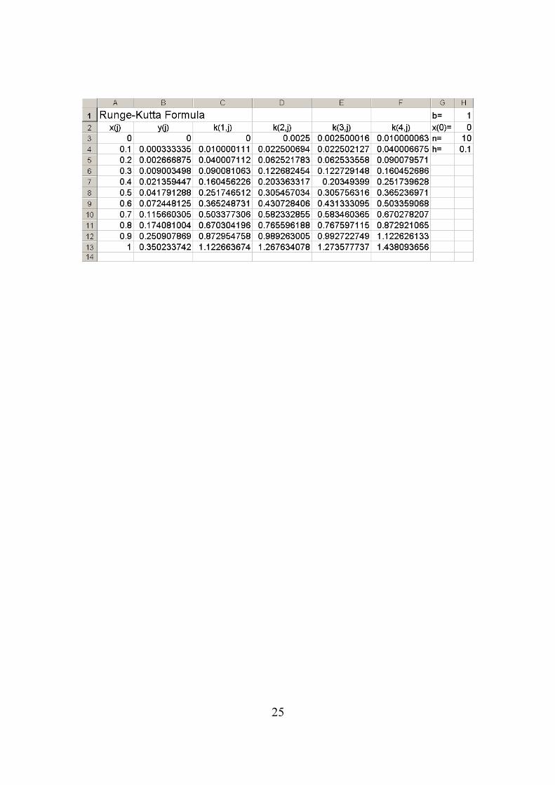
Runge-Kutta Formulaكوتا -) صيغة رونج3( )
( )
( )
1
2 1
3 2
4 3
1 1 2 3 4
,
1 1,
2 2
1 1,
2 2
,
2 26
j j
j j
j j
j j
j j
k f x y
k f x h y h k
k f x h y hk
k f x h y hk
hy y k k k k
+
=
= + +
= + +
= + +
= + + + +
حل المعادلة مثال:( )2 2
, 0 0y x y y′ = + =
]في الفترة ]0,1.
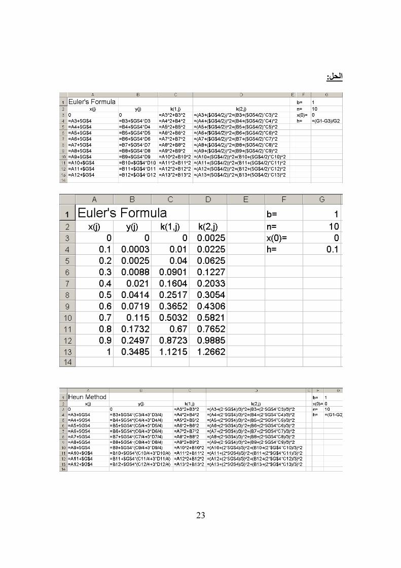
23
الحل:
24
25
26
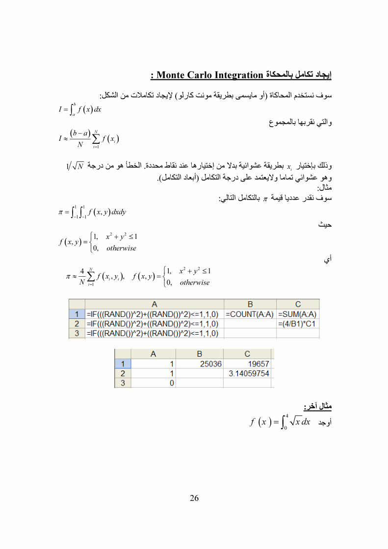
: Monte Carlo Integrationمل بالمحكاة إيجاد تكا
سوف نستخدم المحاكاة (أو مايسمى بطريقة مونت كارلو) إليجاد تكامالت من الشكل:
( )b
a
I f x dx= ∫
والتي نقربها بالمجموع( )
( )1
N
i
i
b aI f x
N=
−
≈ ∑
وذلك بإختيار
ix 1إختيارها عند نقاط محددة. الخطأ هو من درجة بطريقة عشوائية بدال من N
وهو عشوائي تماما واليعتمد على درجة التكامل (أبعاد التكامل). مثال:
بالتكامل التالي: πسوف نقدر عدديا قيمة
( )1 1
1 1
,f x y dxdyπ− −
= ∫ ∫
حيث
( )2 2
1, 1,
0,
x yf x y
otherwise
+ ≤=
أي
( ) ( )2 2
1
1, 14, , ,
0,
N
i i
i
x yf x y f x y
N otherwiseπ
=
+ ≤≈ =
∑
مثال آخر:
)أوجد )4
0
f x x dx= ∫
27
الخطوات:
1رقم عشوائي nنولد -1 2, ,...,
nx x x بحيث( )~ 0,4
ix U لجميع قيمi .
)أوجد -2 )1 1
1 1ˆn n
i i
i i
f f x xn n
= =
= =∑ ∑.
بالعالقة يقرب التكامل -3
( ) ( )
( )4
0
ˆ
ˆ ˆ4 0 4
b
a
f x dx b a f
x dx f f
≈ − ×
≈ − × =
∫
∫
يقدر الخطأ بالعالقة
( )( )
( )
22
2 2
1
ˆ ˆ1ˆ,
n
i
i
f ferror b a f f x
n n=
−
≈ − = ∑
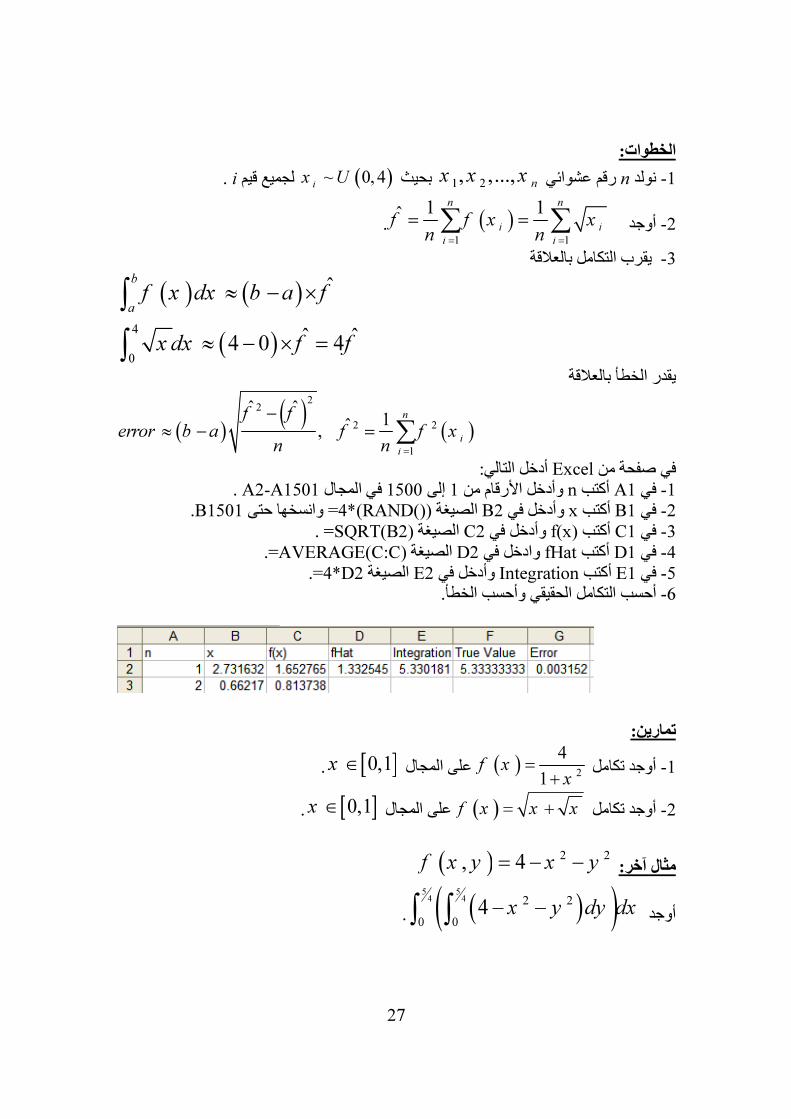
أدخل التالي: Excelفي صفحة من . A2-A1501في المجال 1500إلى 1وأدخل األرقام من nأكتب A1في -1 .B1501وانسخها حتى (()RAND)*4=الصيغة B2وأدخل في xأكتب B1في -2 . SQRT(B2)=الصيغة C2وأدخل في f(x)أكتب C1في -3 .AVERAGE(C:C)=الصيغة D2وادخل في fHatأكتب D1في -4 .D2*4=الصيغة E2وأدخل في Integrationأكتب E1في -5 أحسب التكامل الحقيقي وأحسب الخطأ. -6
تمارين:
)أوجد تكامل -1 )2
4
1f x
x=
+]على المجال ]0,1x ∈.
)أوجد تكامل -2 )f x x x= ]على المجال + ]0,1x ∈.
) مثال آخر: ) 2 2, 4f x y x y= − −
)أوجد )( )5 54 4 2 2
0 0
4 x y dy dx− −∫ ∫.
28
الخطوات:
)نقطة عشوائية nنولد -1 ) ( ) ( )1 1 2 2, , , ,..., ,
n nx y x y x y بحيث( )5~ 0,
4ix U
)و )5~ 0,4i
y U لجميع قيمi .
)أوجد -2 ) 2 2
1 1
1 1ˆ , (4 )n n
i i i i
i i
f f x y x yn n
= =
= = − −∑ ∑.
يقرب التكامل بالعالقة -3
( ) ( ) ( )
( )5 54 4 2 2
0 0
ˆ,
5 5 25ˆ ˆ4 0 04 4 16
b d
a c
f x y dydx b a d c f
x y dydx f f
≈ − × − ×
− − ≈ − × − × =
∫ ∫
∫ ∫
يقدر الخطأ بالعالقة
( ) ( )( )
( )
22
2 2
1
ˆ ˆ1ˆ, ,
n
i i
i
f ferror b a d c f f x y
n n=
−
≈ − × − = ∑
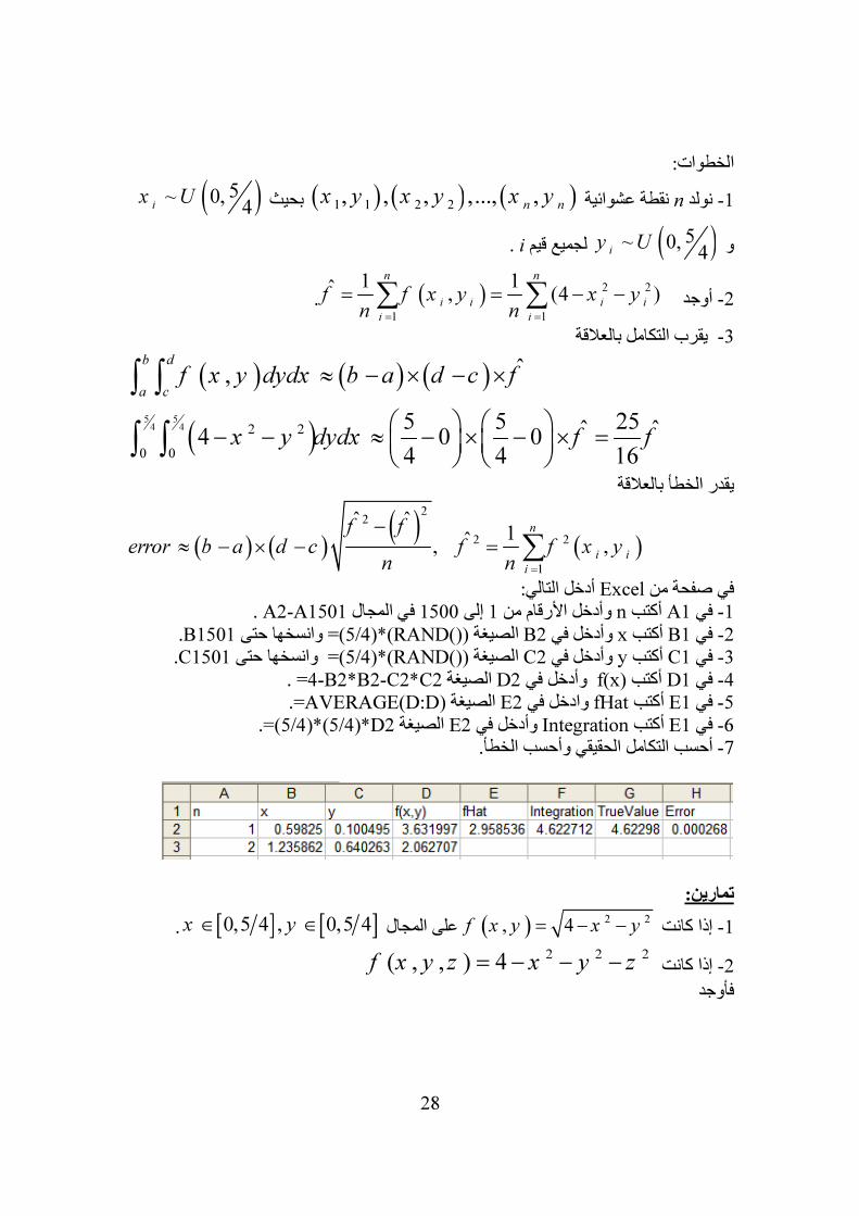
أدخل التالي: Excelفي صفحة من . A2-A1501في المجال 1500إلى 1ل األرقام من وأدخ nأكتب A1في -1 .B1501وانسخها حتى (()RAND)*(5/4)=الصيغة B2وأدخل في xأكتب B1في -2 .C1501وانسخها حتى (()RAND)*(5/4)=الصيغة C2وأدخل في yأكتب C1في -3 . B2*B2-C2*C2-4=الصيغة D2وأدخل في f(x)أكتب D1في -4 .AVERAGE(D:D)=الصيغة E2وادخل في fHatأكتب E1في - 5 .D2*(5/4)*(5/4)=الصيغة E2وأدخل في Integrationأكتب E1في - 6 أحسب التكامل الحقيقي وأحسب الخطأ. - 7
تمارين:
)إذا كانت -1 ) 2 2, 4f x y x y= − ]على المجال − ] [ ]0,5 4 , 0,5 4x y∈ ∈.
إذا كانت -22 2 2( , , ) 4f x y z x y z= − − −
فأوجد
29
( )( )( )9 10 1 11 102 2 2
0 0 0
4 x y z dz dy dx− − −∫ ∫ ∫
. 2.9634القيمة الحقيقية =
)إذا كانت -3 ) 2 2 2 2, , , 5f x y z u x y z u= − − − فأوجد −
( )( )( )4 5 9 10 1 11 102 2 2 2
0 0 0 0
5 x y z u du dz dy dx − − − − ∫ ∫ ∫ ∫
. 2.99663القيمة الحقيقية =
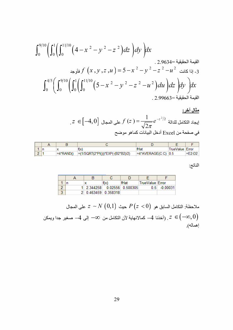
مثال آخر:
إيجاد التكامل للدالة 221
( )2
zf z eπ
−
]على المجال = ]4,0z ∈ −.
أدخل البيانات كماهو موضح Excelفي صفحة من
الناتج:
)مالحظة: التكامل السابق هو )0P z )حيث > )0,1z N∼ على المجال
( ),0z ∈ صغير جدا ويمكن −4إلى ∞−التكامل من كماالنهاية ألن −4. (أخذنا ∞−
إهماله).
30
الفصل الثاني
في حل مسائل البرمجة الرياضية: EXCEL SOLVERإستخدام
لحل مسائل في البرمجة الخطية والعددية EXCEL SOLVERفي هذا الفصل سوف نستخدم
ة. سوف نستعرض ذلك على مسائل متنوعة من مختلف المراجع المذكورة آخر والتربيعية والحركي الكتاب.
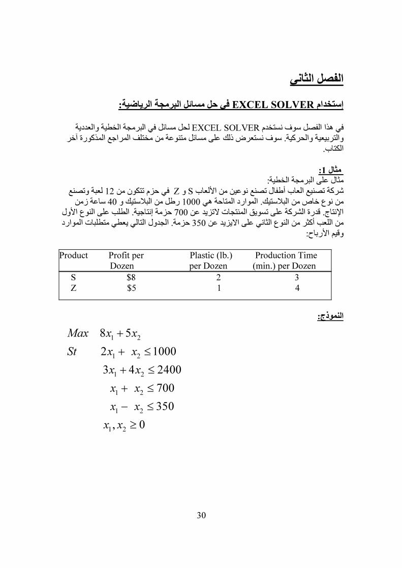
: 1مثال
مثال على البرمجة الخطية:لعبة وتصنع 12في حزم تتكون من Zو Sشركة تصنيع العاب أطفال تصنع نوعين من األلعاب
ساعة زمن 40و رطل من البالستيك 1000من نوع خاص من البالستيك. الموارد المتاحة هي حزمة إنتاجية. الطلب على النوع األول 700اإلنتاج. قدرة الشركة على تسويق المنتجات التزيد عن
حزمة. الجدول التالي يعطي متطلبات الموارد 350من اللعب أكثر من النوع الثاني على االيزيد عن وقيم األرباح:
Product Profit per Plastic (lb.) Production Time Dozen per Dozen (min.) per Dozen S $8 2 3 Z $5 1 4
النموذج:
1 2
1 2
1 2
1 2
1 2
1 2
8 5
2 1000
3 4 2400
700
350
, 0
Max x x
St x x
x x
x x
x x
x x
+
+ ≤
+ ≤
+ ≤
− ≤
≥
31
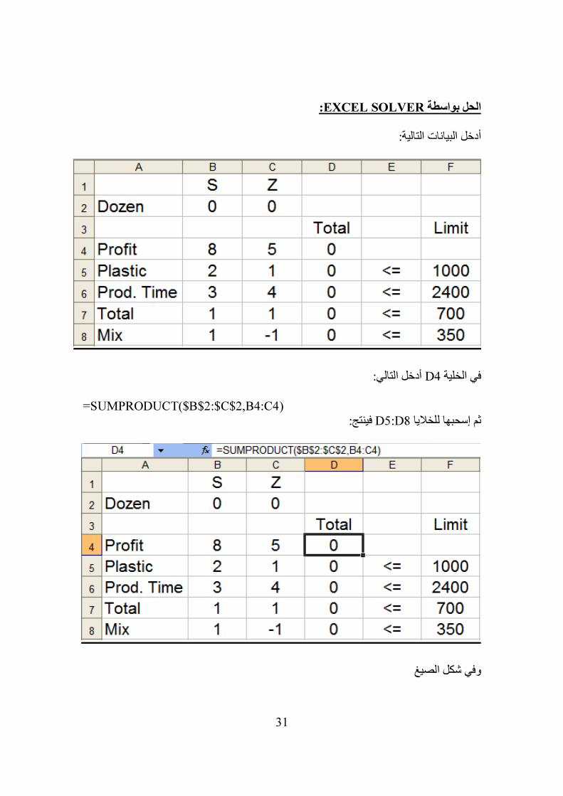
:EXCEL SOLVERالحل بواسطة
أدخل البيانات التالية:
أدخل التالي: D4في الخلية =SUMPRODUCT($B$2:$C$2,B4:C4)
فينتج: D5:D8ثم إسحبها للخاليا
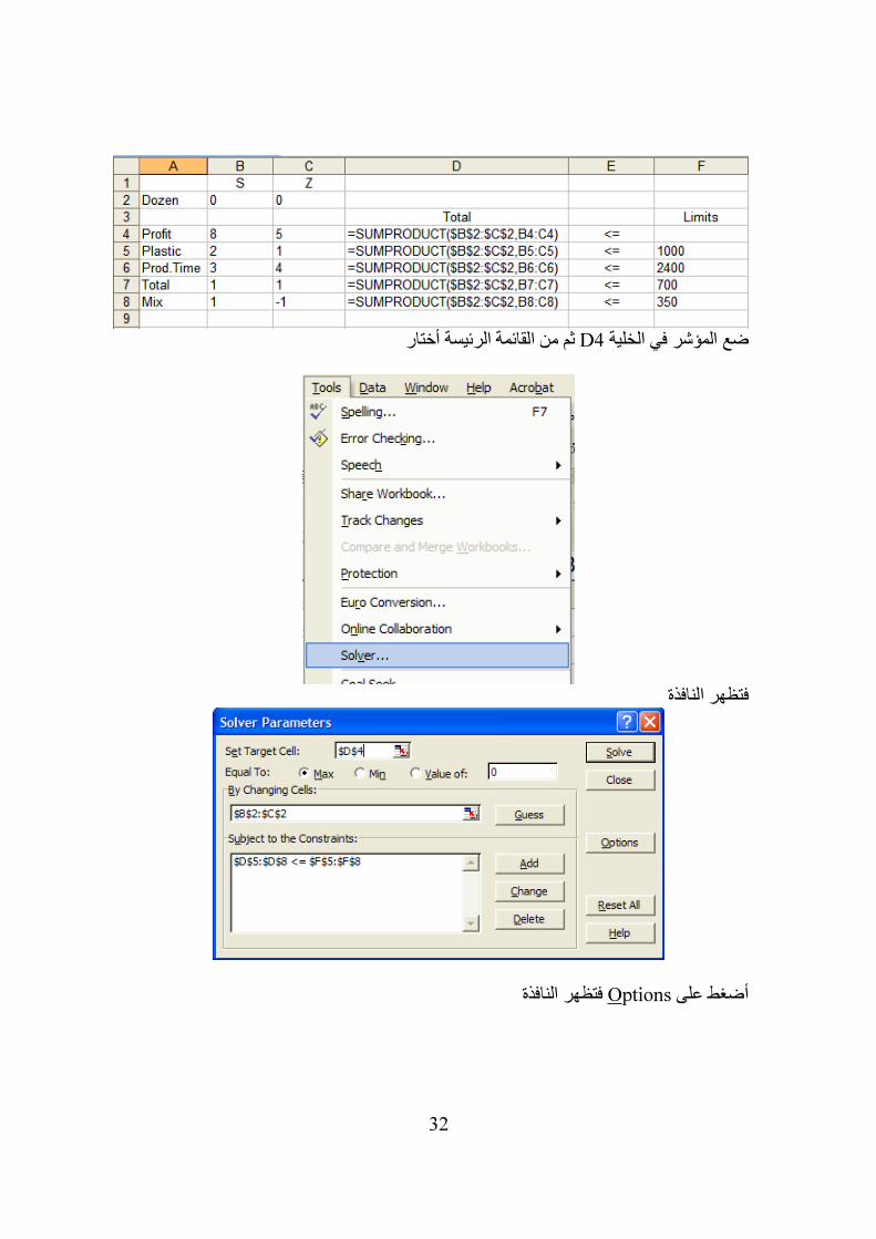
وفي شكل الصيغ
32
ثم من القائمة الرئيسة أختار D4لخلية ضع المؤشر في ا
فتظهر النافذة
فتظهر النافذة ptionsOأضغط على
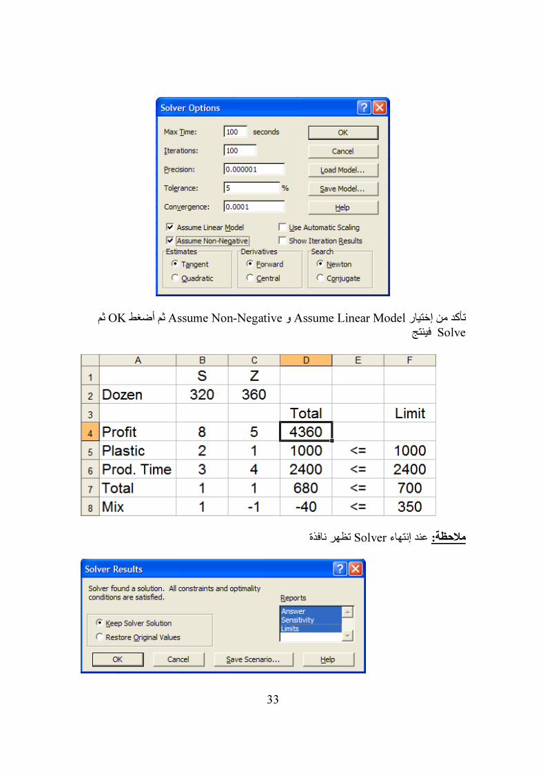
33
ثم OKثم أضغط Assume Non-Negativeو Assume Linear Modelتأكد من إختيار Solve فينتج
تظهر نافذة Solverعند إنتهاء مالحظة:
34
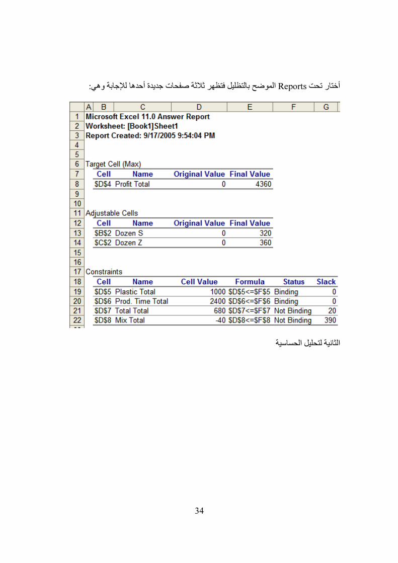
الموضح بالتظليل فتظهر ثالثة صفحات جديدة أحدها لإلجابة وهي: Reportsحت أختار ت
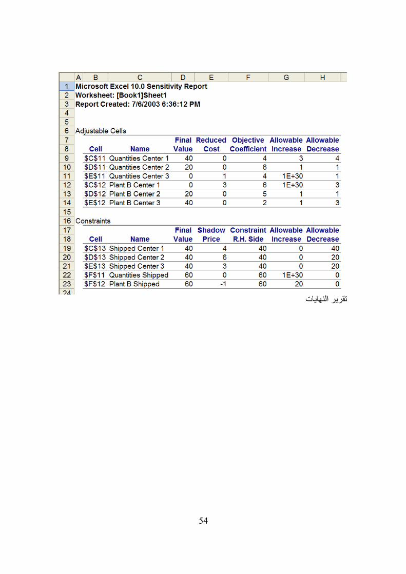
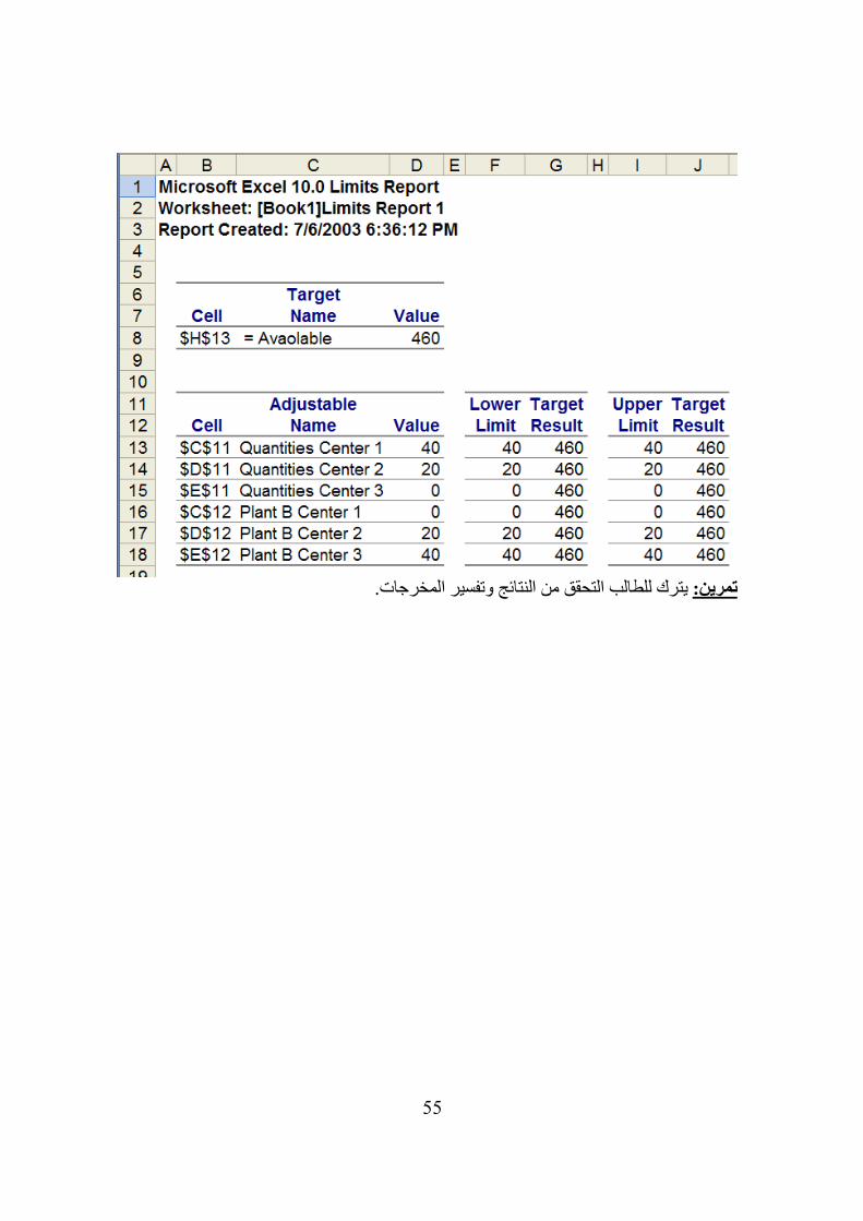
الثانية لتحليل الحساسية
35
والثالثة للنهايات
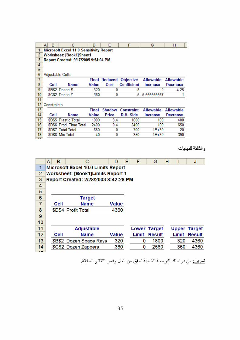
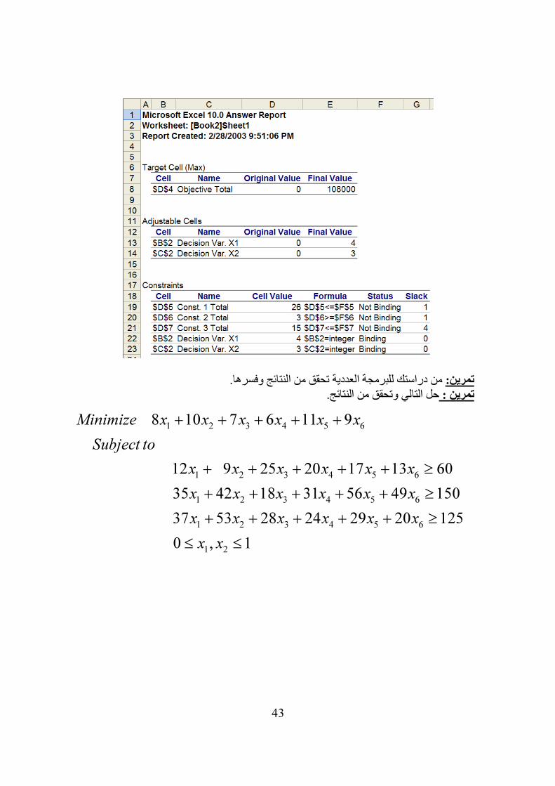
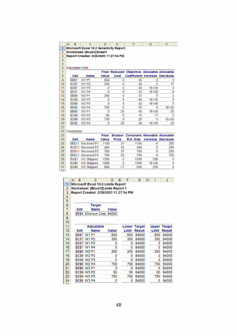
من دراستك للبرمجة الخطية تحقق من الحل وفسر النتائج السابقة. تمرين:
36
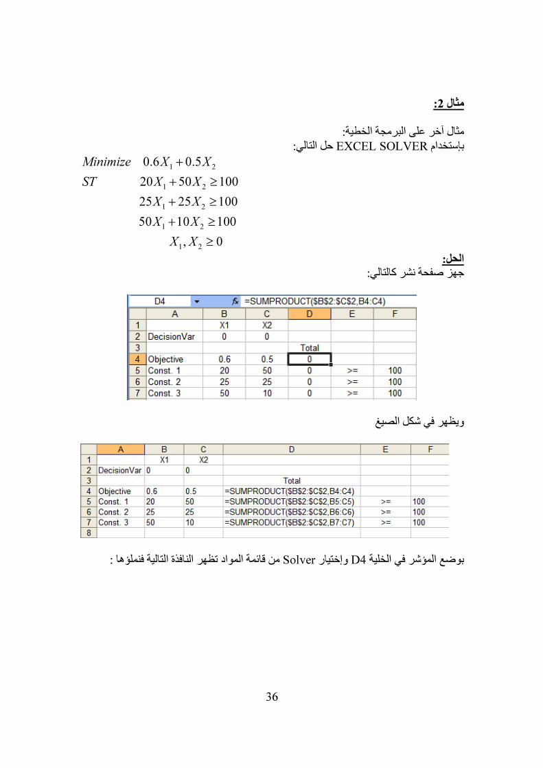
:2مثال
مثال آخر على البرمجة الخطية: حل التالي: EXCEL SOLVERبإستخدام
1 2
1 2
1 2
1 2
1 2
0.6 0.5
20 50 100
25 25 100
50 10 100
, 0
Minimize X X
ST X X
X X
X X
X X
+
+ ≥
+ ≥
+ ≥
≥
الحل: جهز صفحة نشر كالتالي:
ويظهر في شكل الصيغ
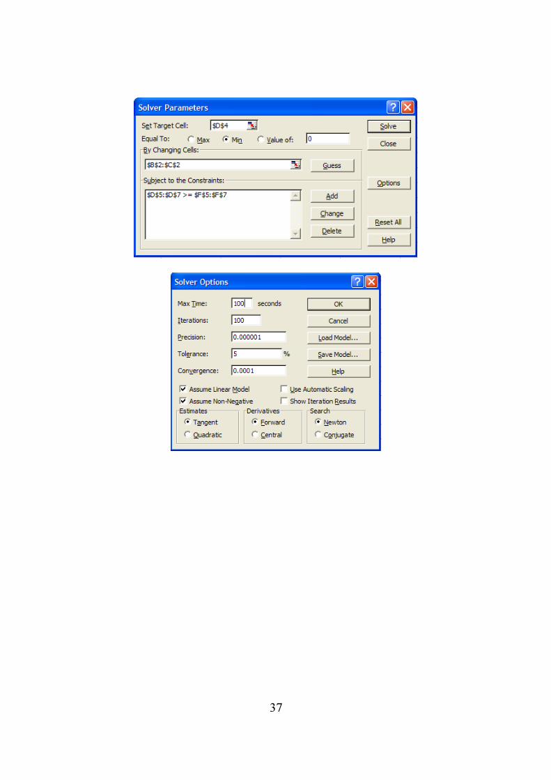
من قائمة المواد تظهر النافذة التالية فنملؤها : Solverوإختيار D4بوضع المؤشر في الخلية
37
38
39
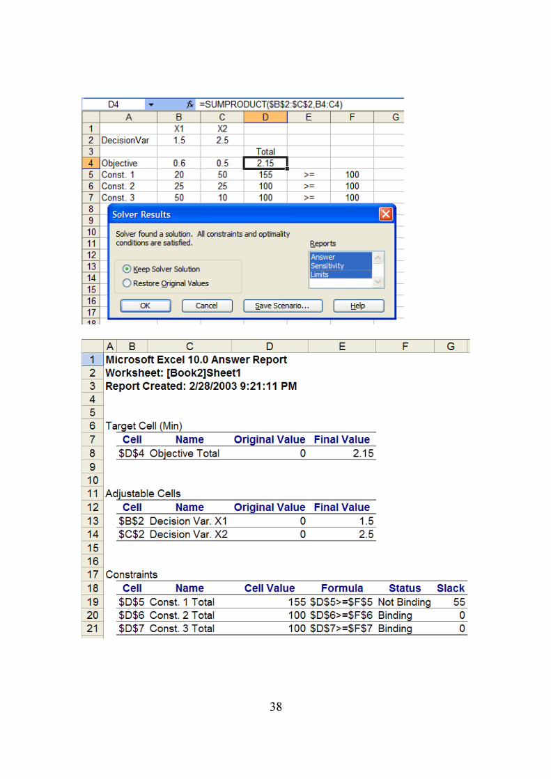
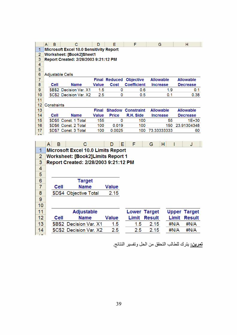
يترك للطالب التحقق من الحل وتفسير النتائج. :تمرين
40
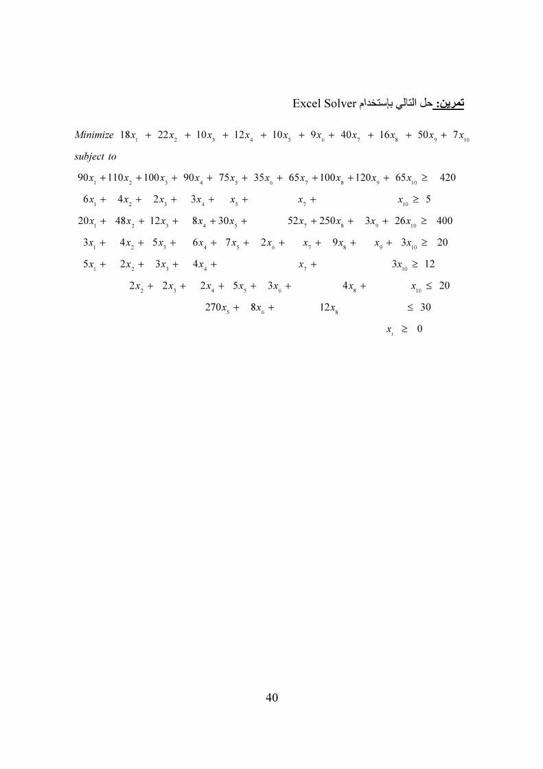
Excel Solverحل التالي بإستخدام تمرين:
1 2 3 4 5 6 7 8 9 10
1 2 3 4 5 6 7 8 9 10
1 2 3 4 5
18 22 10 12 10 9 40 16 50 7
90 110 100 90 75 35 65 100 120 65 420
6 4 2 3
Minimize x x x x x x x x x x
subject to
x x x x x x x x x x
x x x x x
+ + + + + + + + +
+ + + + + + + + + ≥
+ + + + +7 10
1 2 3 4 5 7 8 9 10
1 2 3 4 5 6 7 8 9 10
5
20 48 12 8 30 52 250 3 26 400
3 4 5 6 7 2 9 3 20
x x
x x x x x x x x x
x x x x x x x x x x
+ ≥
+ + + + + + + + ≥
+ + + + + + + + + ≥
1 2 3 4 7 10
2 3 4 5 6 8 10
5 2 3 4 3 12
2 2 2 5 3 4 20
x x x x x x
x x x x x x x
+ + + + + ≥
+ + + + + + ≤
5 6 8 270 8 12 30
x x x+ + ≤
0ix ≥
41
:3مثال Integer Programmingالبرمجة العددية الصحيحة
حل التالي:1 2
1 2
2
1 2
1 2
. 12000 20000
. 2 6 27
2
3 19
, 0 and integers
Max X X
St X X
X
X X
X X
+
+ ≤
≥
+ ≤
≥
42
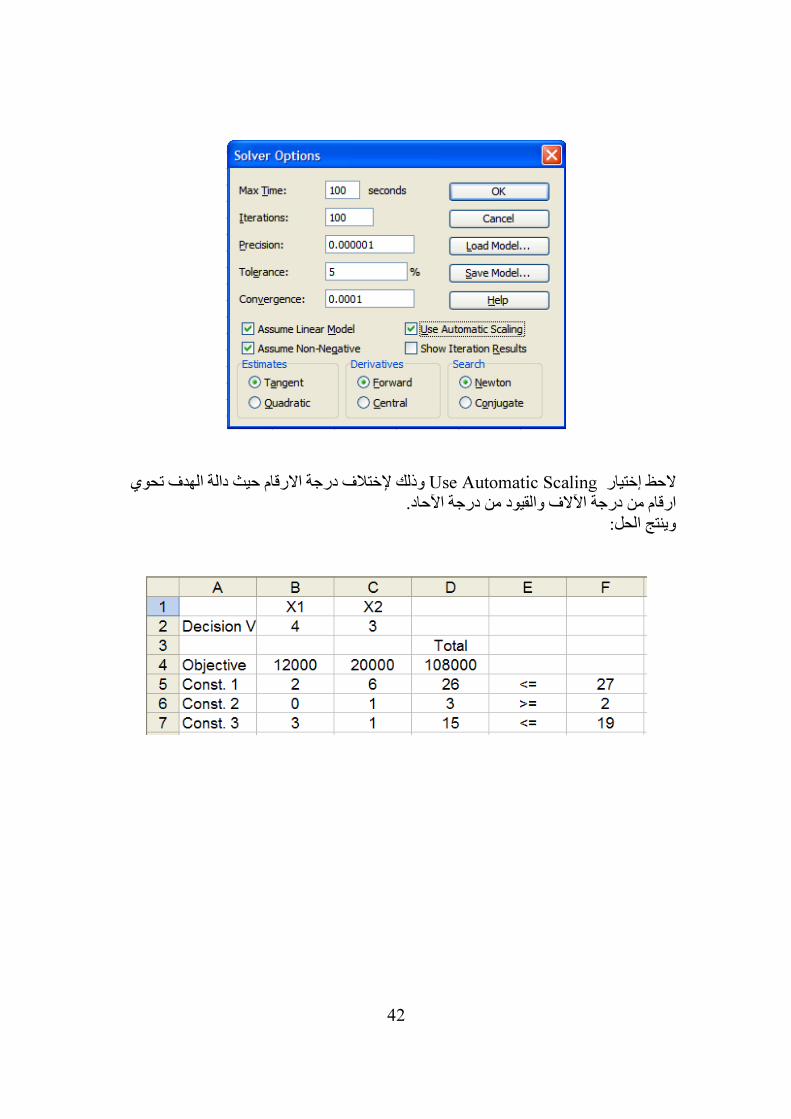
م حيث دالة الهدف تحوي وذلك إلختالف درجة االرقا Use Automatic Scalingالحظ إختيار ارقام من درجة اآلالف والقيود من درجة اآلحاد.
وينتج الحل:
43
من دراستك للبرمجة العددية تحقق من النتائج وفسرها. تمرين: حل التالي وتحقق من النتائج. :تمرين
1 2 3 4 5 6
1 2 3 4 5 6
1 2 3 4 5 6
1 2 3 4 5 6
1 2
8 10 7 6 11 9
12 9 25 20 17 13 60
35 42 18 31 56 49 150
37 53 28 24 29 20 125
0 , 1
Minimize x x x x x x
Subject to
x x x x x x
x x x x x x
x x x x x x
x x
+ + + + +
+ + + + + ≥
+ + + + + ≥
+ + + + + ≥
≤ ≤

44
: 4مثال مثال على الشبكات والنقل:
حل مشكلة النقل للشبكة التالية:
P1
P2
P3
W1
W2
W3
W4
35
30
32
37
40
42
25
40
15
20
28
Plant
Warehoise
S1=1200
S2=1000
S3=800
D1=1100
D2=400
D3=750
D4=750
40
والتي نشكلها على شكل البرمجة الخطية التالية( )Total Shipping Cost
:
Amount shipped from each source Supply at that source
Amount received at each destination = Demand at that destination
No negative shipments
Min
St
≤
إذا رمزنا بـ ij
X 1,2,3لعدد الوحدات التي تشحن من المصنعi 1,2,3,4jإلى المخزن = فتكتب = ل:المشكلة على الشك
11 12 13 14 21 22 23 24 31 32 33 34
11 12 13 14
35 20 40 32 37 40 42 25 40 15 20 28
Min X X X X X X X X X X X X
St X X X X
+ + + + + + + + + + +
+ + +
21 22 23 24
1200
1000
X X X X
≤
+ + + ≤
31 32 33 34
11 21
800
+
X X X X
X X
+ + + ≤
+31
12 22 32
=1100
+ +
X
X X X
13 23 33
=400
+ + =750
X X X
14 24 34 + + 750
X X X =
0,ij
X for all i and j≥
45
شكل الصيغ
Solverوبإستخدام
46
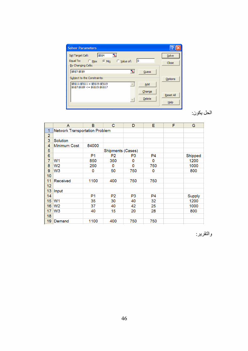
الحل يكون:
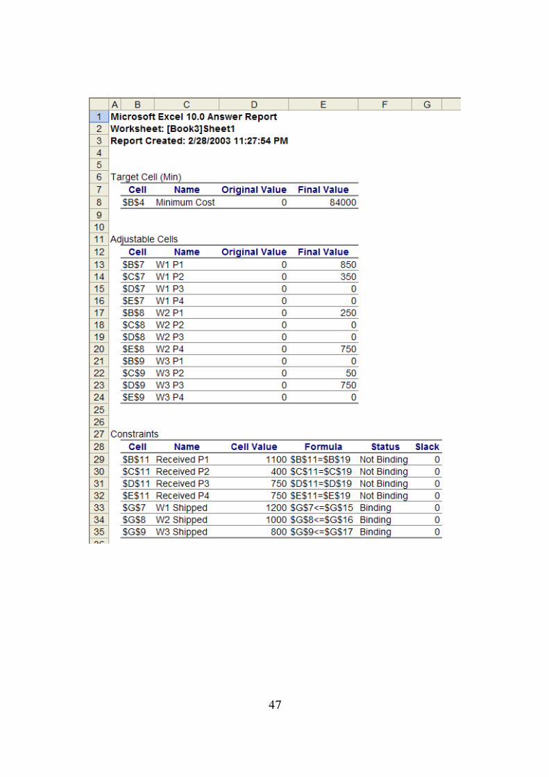
والتقرير:
47
48

49
يترك للطالب التحقق من النتائج وتفسير المخرجات. تمرين:
50
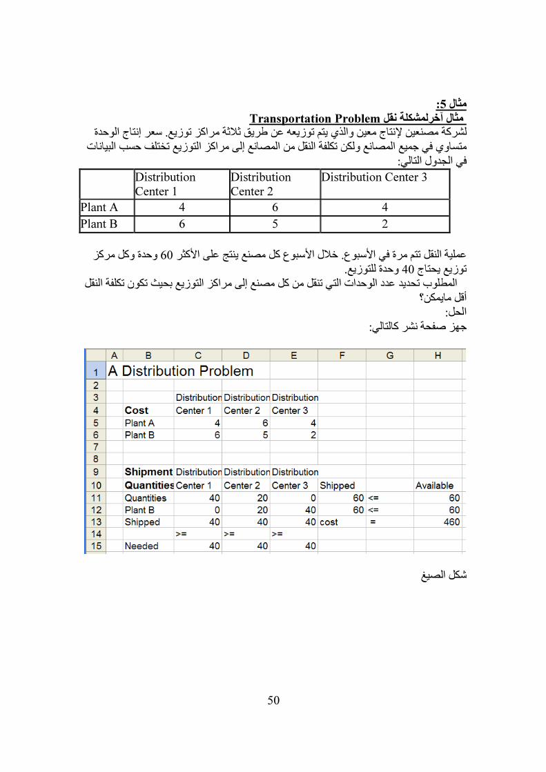
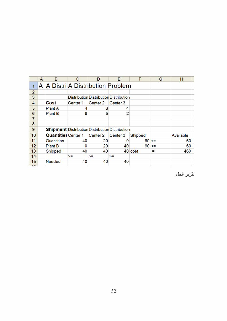
:5مثال Transportation Problemمثال آخرلمشكلة نقل
معين والذي يتم توزيعه عن طريق ثالثة مراكز توزيع. سعر إنتاج الوحدة لشركة مصنعين إلنتاجمتساوي في جميع المصانع ولكن تكلفة النقل من المصانع إلى مراكز التوزيع تختلف حسب البيانات
في الجدول التالي: Distribution
Center 1 Distribution Center 2
Distribution Center 3
Plant A 4 6 4 Plant B 6 5 2
وحدة وكل مركز 60عملية النقل تتم مرة في األسبوع. خالل األسبوع كل مصنع ينتج على األكثر
وحدة للتوزيع. 40توزيع يحتاج المطلوب تحديد عدد الوحدات التي تنقل من كل مصنع إلى مراكز التوزيع بحيث تكون تكلفة النقل
أقل مايمكن؟ الحل:
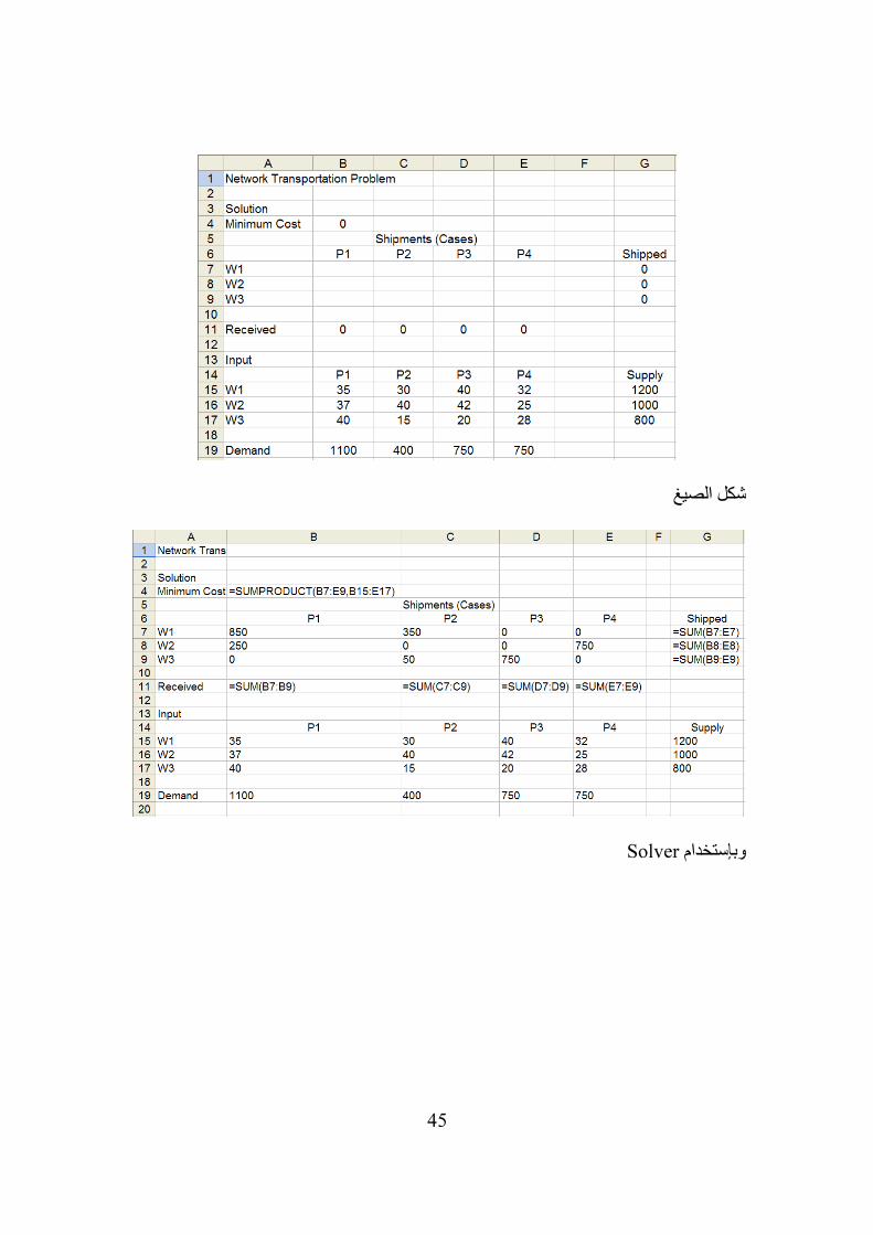
تالي:جهز صفحة نشر كال
شكل الصيغ

51
وعبئ البيانات كالتالي: SOLVERأفتح
ينتج الحل Solveوبالضغط على
52
تقرير الحل
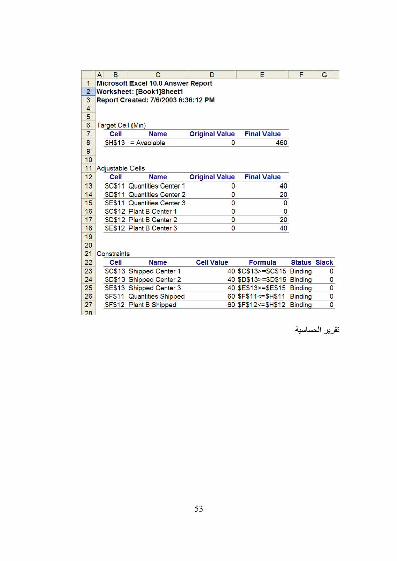
53
تقرير الحساسية
54
تقرير النهايات
55
يترك للطالب التحقق من النتائج وتفسير المخرجات. تمرين:
56
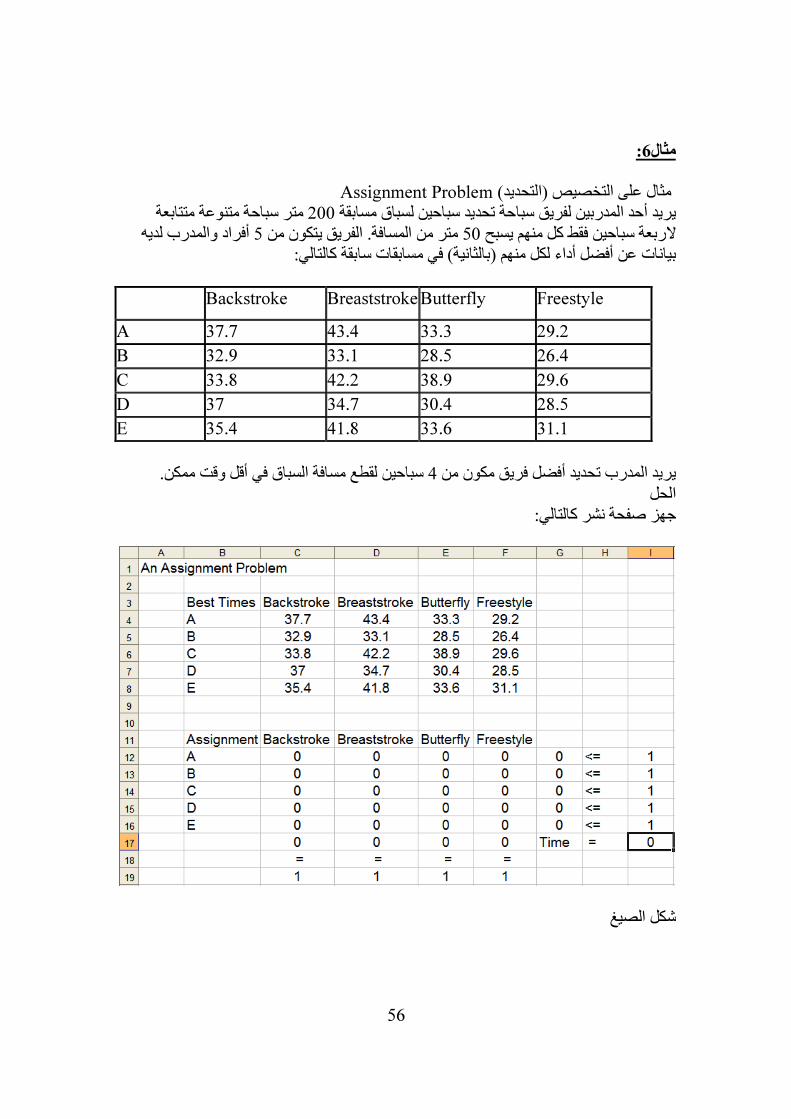
:6مثال Assignment Problemمثال على التخصيص (التحديد)
متر سباحة متنوعة متتابعة 200ديد سباحين لسباق مسابقة يريد أحد المدربين لفريق سباحة تحأفراد والمدرب لديه 5متر من المسافة. الفريق يتكون من 50الربعة سباحين فقط كل منهم يسبح
بيانات عن أفضل أداء لكل منهم (بالثانية) في مسابقات سابقة كالتالي:
Backstroke Breaststroke Butterfly Freestyle
A 37.7 43.4 33.3 29.2 B 32.9 33.1 28.5 26.4 C 33.8 42.2 38.9 29.6 D 37 34.7 30.4 28.5 E 35.4 41.8 33.6 31.1
سباحين لقطع مسافة السباق في أقل وقت ممكن. 4يريد المدرب تحديد أفضل فريق مكون من
الحل جهز صفحة نشر كالتالي:
صيغشكل ال
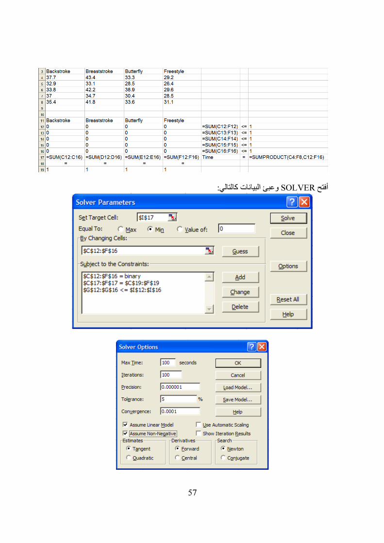
57
وعبئ البيانات كالتالي: SOLVERأفتح
58
ينتج الحل Solveوبالضغط على
تقرير الحل
59
من النتائج وتفسير المخرجات.يترك للطالب التحقق تمرين:
60
:7مثال :Assignment Problemمثال تخصيص
:الجدول التالي يمثل زمن النقل من خطوط التجميع إلى مناطق الفحص لقطع إلكترونية Inspection Area
AssemblyLine
A B C D E
1 10 4 6 10 12
2 11 7 7 9 14
3 13 8 12 14 15
4 14 16 13 17 17
5 19 11 17 20 19
المطلوب هو تحديد الكيفية التي تنقل بها القطع من خطوط اإلنتاج إلى مناطق الفحص في أقل زمن ممكن مع مالحظة أن يخصص خط تجميع واحد لمنطقة فحص واحدة.
جهز صفحة نشر كالتالي:
شكل الصيغ
61
وعبئ البيانات كالتالي: SOLVERأفتح
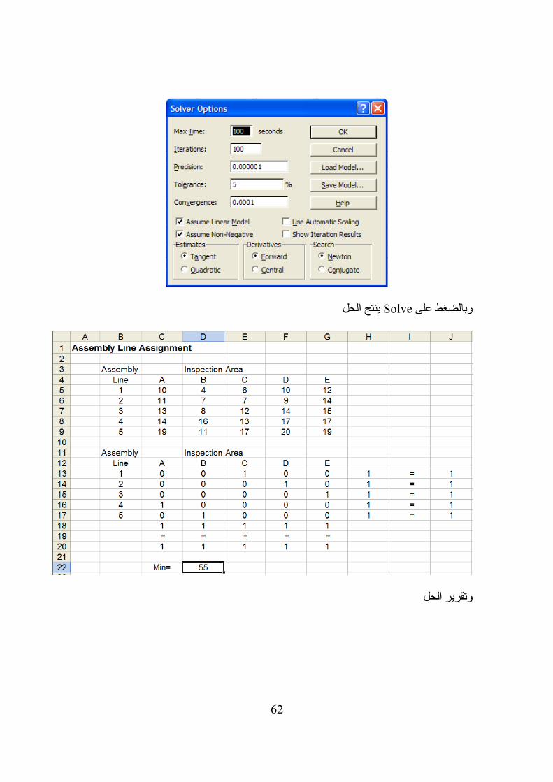
62
ينتج الحل Solveوبالضغط على
وتقرير الحل
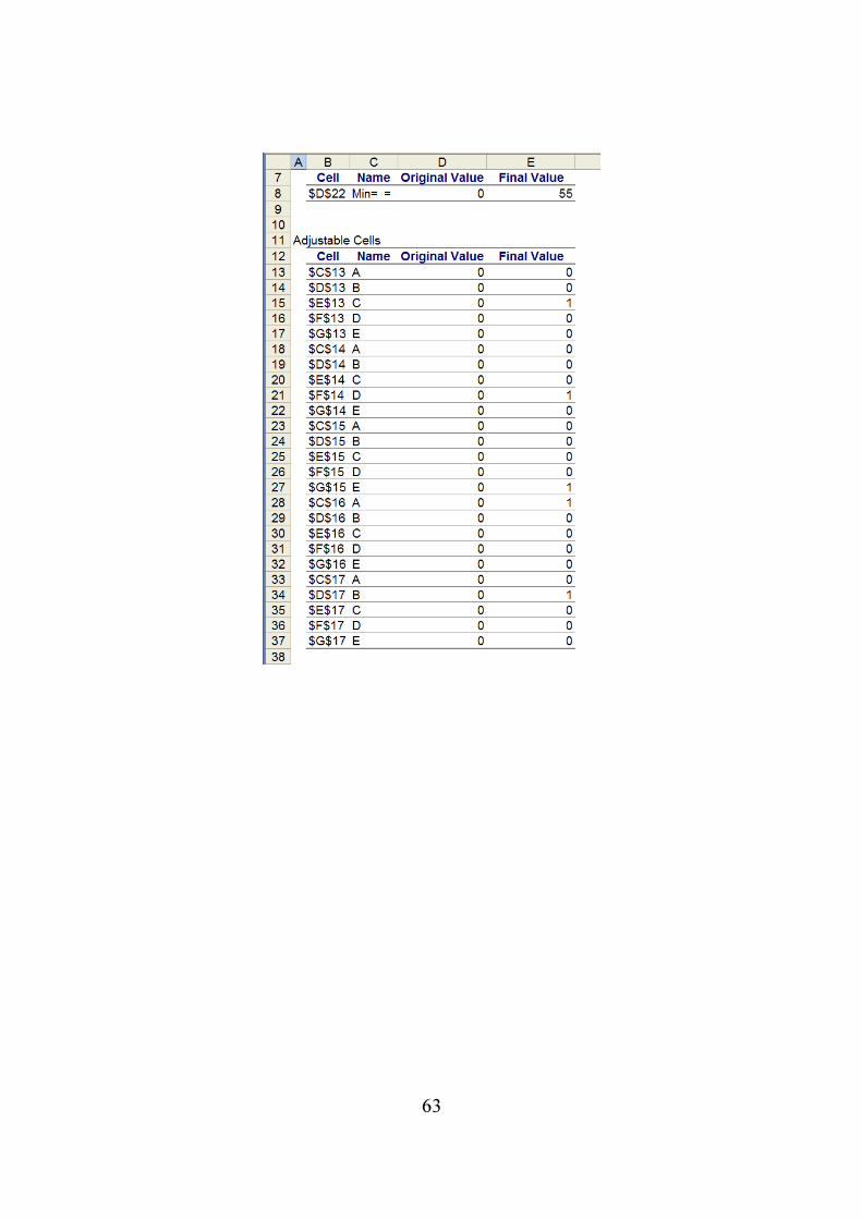
63
64
:8 مثال
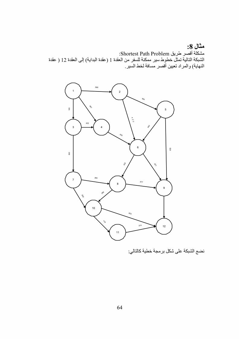
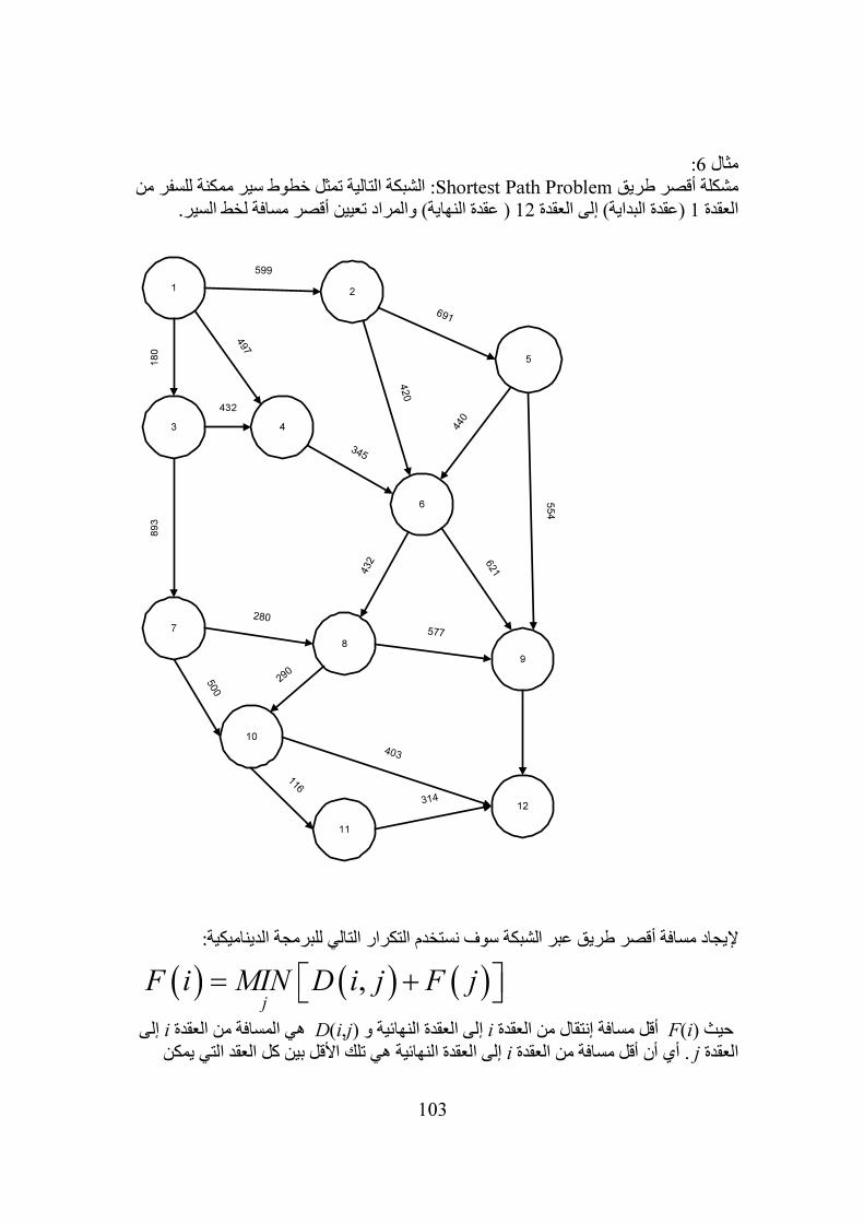
:Shortest Path Problemمشكلة أقصر طريق ( عقدة 12(عقدة البداية) إلى العقدة 1الشبكة التالية تمثل خطوط سير ممكنة للسفر من العقدة
النهاية) والمراد تعيين أقصر مسافة لخط السير.
12
3 4
5
6
7
8
9
10
11
12
599
180
497
432
345
42
0
440
691
893
280
500
290
577
116
403
314
432 6
21
554
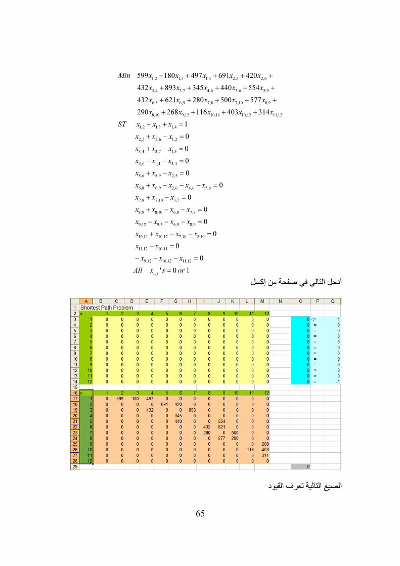
نضع الشبكة على شكل برمجة خطية كالتالي:
65
1,2 1,3 1,4 2,5 2,6
3,4 3,7 4,6 5,6 5,9
6,8 6,9 7,8 7,10 8,9
8,10 9,12 10,11 10,12 11,12
1,2 1,3 1,4
2,5 2,6
599 180 497 691 420
432 893 345 440 554
432 621 280 500 577
290 268 116 403 314
1
Min x x x x x
x x x x x
x x x x x
x x x x x
ST x x x
x x x
+ + + + +
+ + + + +
+ + + + +
+ + + +
+ + =
+ −1,2
3,4 3,7 1,3
4,6 1,4 3,4
5,6 5,9 2,5
6,8 6,9 2,6 4,6 5,6
7,8 7,10 3,7
8,9 8,10 6,8 7,8
9,12 9,5 6,9 8,9
10,11 10,12 7,10 8,10
11,12 10,11
9,12 10,12 11,
0
0
0
0
0
0
0
0
0
0
x x x
x x x
x x x
x x x x x
x x x
x x x x
x x x x
x x x x
x x
x x x
=
+ − =
− − =
+ − =
+ − − − =
+ − =
+ − − =
− − − =
+ − − =
− =
− − −12
,
0
' 0 1i j
All x s or
=
=
أدخل التالي في صفحة من إكسل
الصيغ التالية تعرف القيود
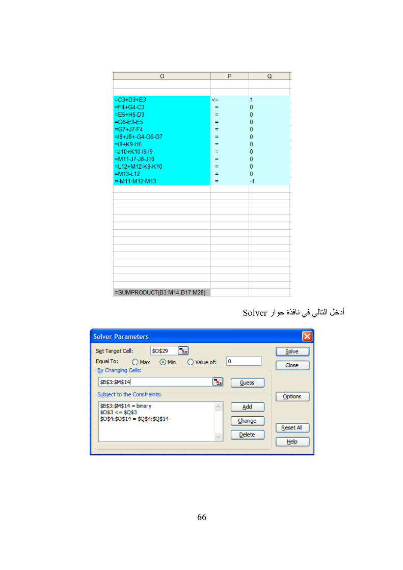
66
Solverأدخل التالي في نافذة حوار
67
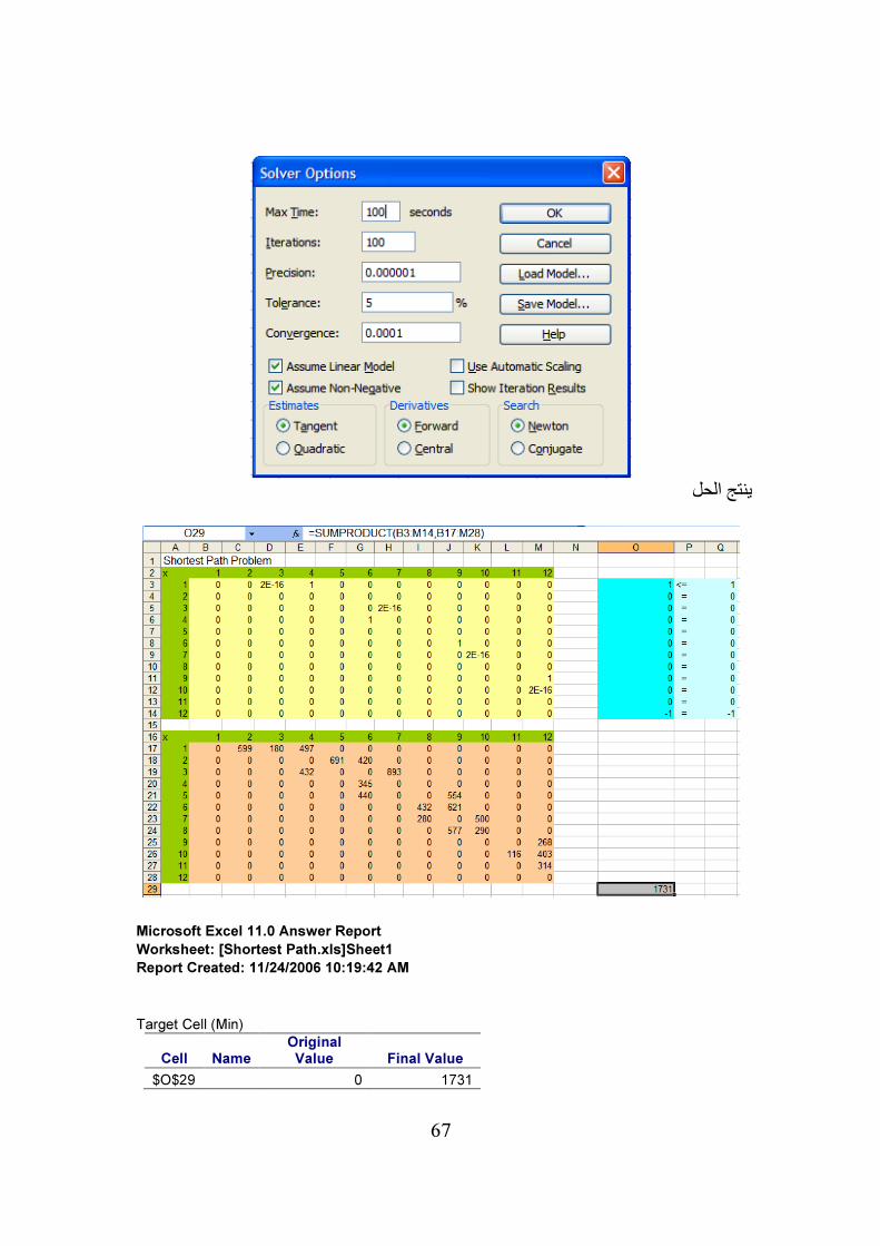
ينتج الحل
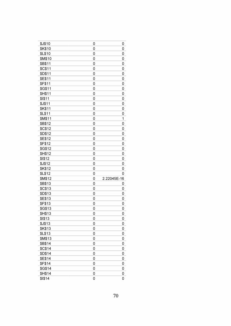
Microsoft Excel 11.0 Answer Report
Worksheet: [Shortest Path.xls]Sheet1
Report Created: 11/24/2006 10:19:42 AM
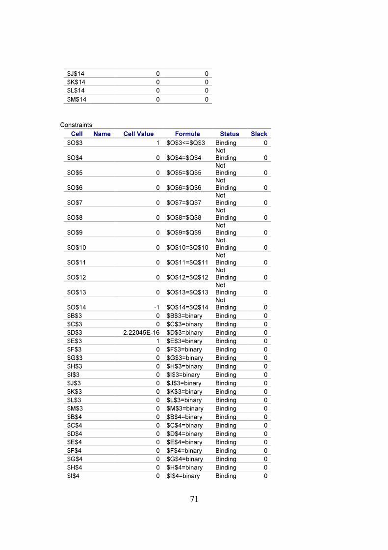
Target Cell (Min)
Cell Name Original Value Final Value
$O$29 0 1731
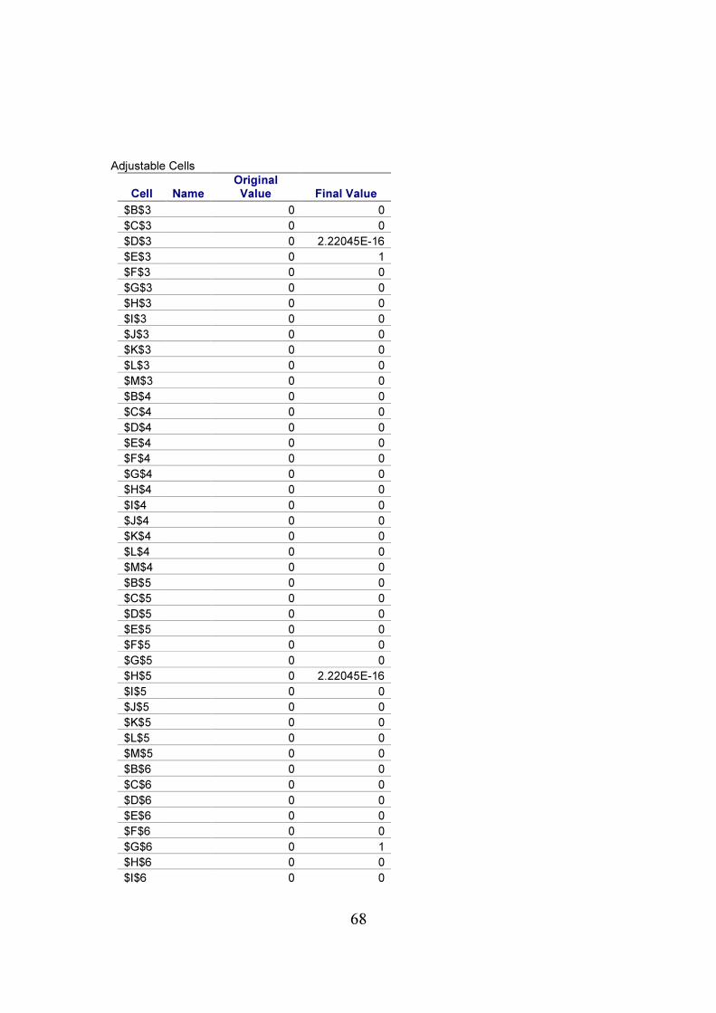
68
Adjustable Cells
Cell Name Original Value Final Value
$B$3 0 0
$C$3 0 0
$D$3 0 2.22045E-16
$E$3 0 1
$F$3 0 0
$G$3 0 0
$H$3 0 0
$I$3 0 0
$J$3 0 0
$K$3 0 0
$L$3 0 0
$M$3 0 0
$B$4 0 0
$C$4 0 0
$D$4 0 0
$E$4 0 0
$F$4 0 0
$G$4 0 0
$H$4 0 0
$I$4 0 0
$J$4 0 0
$K$4 0 0
$L$4 0 0
$M$4 0 0
$B$5 0 0
$C$5 0 0
$D$5 0 0
$E$5 0 0
$F$5 0 0
$G$5 0 0
$H$5 0 2.22045E-16
$I$5 0 0
$J$5 0 0
$K$5 0 0
$L$5 0 0
$M$5 0 0
$B$6 0 0
$C$6 0 0
$D$6 0 0
$E$6 0 0
$F$6 0 0
$G$6 0 1
$H$6 0 0
$I$6 0 0
69
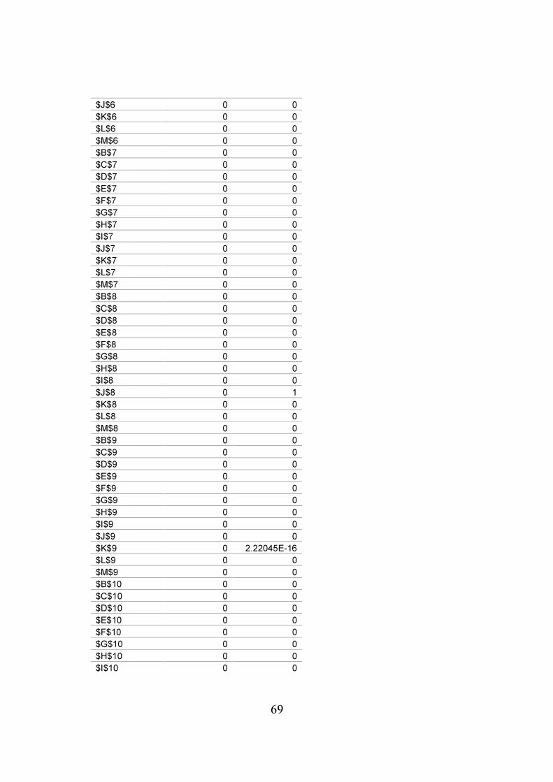
$J$6 0 0
$K$6 0 0
$L$6 0 0
$M$6 0 0
$B$7 0 0
$C$7 0 0
$D$7 0 0
$E$7 0 0
$F$7 0 0
$G$7 0 0
$H$7 0 0
$I$7 0 0
$J$7 0 0
$K$7 0 0
$L$7 0 0
$M$7 0 0
$B$8 0 0
$C$8 0 0
$D$8 0 0
$E$8 0 0
$F$8 0 0
$G$8 0 0
$H$8 0 0
$I$8 0 0
$J$8 0 1
$K$8 0 0
$L$8 0 0
$M$8 0 0
$B$9 0 0
$C$9 0 0
$D$9 0 0
$E$9 0 0
$F$9 0 0
$G$9 0 0
$H$9 0 0
$I$9 0 0
$J$9 0 0
$K$9 0 2.22045E-16
$L$9 0 0
$M$9 0 0
$B$10 0 0
$C$10 0 0
$D$10 0 0
$E$10 0 0
$F$10 0 0
$G$10 0 0
$H$10 0 0
$I$10 0 0
70
$J$10 0 0
$K$10 0 0
$L$10 0 0
$M$10 0 0
$B$11 0 0
$C$11 0 0
$D$11 0 0
$E$11 0 0
$F$11 0 0
$G$11 0 0
$H$11 0 0
$I$11 0 0
$J$11 0 0
$K$11 0 0
$L$11 0 0
$M$11 0 1
$B$12 0 0
$C$12 0 0
$D$12 0 0
$E$12 0 0
$F$12 0 0
$G$12 0 0
$H$12 0 0
$I$12 0 0
$J$12 0 0
$K$12 0 0
$L$12 0 0
$M$12 0 2.22045E-16
$B$13 0 0
$C$13 0 0
$D$13 0 0
$E$13 0 0
$F$13 0 0
$G$13 0 0
$H$13 0 0
$I$13 0 0
$J$13 0 0
$K$13 0 0
$L$13 0 0
$M$13 0 0
$B$14 0 0
$C$14 0 0
$D$14 0 0
$E$14 0 0
$F$14 0 0
$G$14 0 0
$H$14 0 0
$I$14 0 0
71
$J$14 0 0
$K$14 0 0
$L$14 0 0
$M$14 0 0
Constraints
Cell Name Cell Value Formula Status Slack
$O$3 1 $O$3<=$Q$3 Binding 0
$O$4 0 $O$4=$Q$4 Not Binding 0
$O$5 0 $O$5=$Q$5 Not Binding 0
$O$6 0 $O$6=$Q$6 Not Binding 0
$O$7 0 $O$7=$Q$7 Not Binding 0
$O$8 0 $O$8=$Q$8 Not Binding 0
$O$9 0 $O$9=$Q$9 Not Binding 0
$O$10 0 $O$10=$Q$10 Not Binding 0
$O$11 0 $O$11=$Q$11 Not Binding 0
$O$12 0 $O$12=$Q$12 Not Binding 0
$O$13 0 $O$13=$Q$13 Not Binding 0
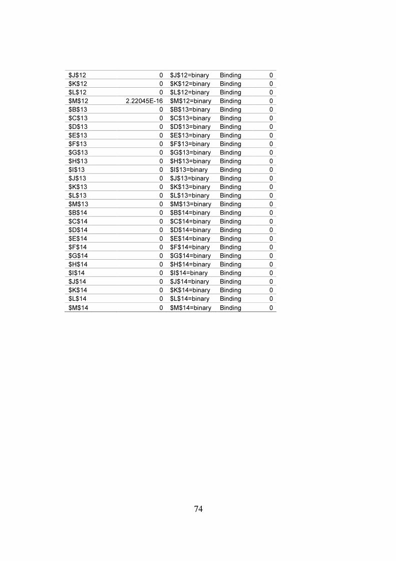
$O$14 -1 $O$14=$Q$14 Not Binding 0
$B$3 0 $B$3=binary Binding 0
$C$3 0 $C$3=binary Binding 0
$D$3 2.22045E-16 $D$3=binary Binding 0
$E$3 1 $E$3=binary Binding 0
$F$3 0 $F$3=binary Binding 0
$G$3 0 $G$3=binary Binding 0
$H$3 0 $H$3=binary Binding 0
$I$3 0 $I$3=binary Binding 0
$J$3 0 $J$3=binary Binding 0
$K$3 0 $K$3=binary Binding 0
$L$3 0 $L$3=binary Binding 0
$M$3 0 $M$3=binary Binding 0
$B$4 0 $B$4=binary Binding 0
$C$4 0 $C$4=binary Binding 0
$D$4 0 $D$4=binary Binding 0
$E$4 0 $E$4=binary Binding 0
$F$4 0 $F$4=binary Binding 0
$G$4 0 $G$4=binary Binding 0
$H$4 0 $H$4=binary Binding 0
$I$4 0 $I$4=binary Binding 0
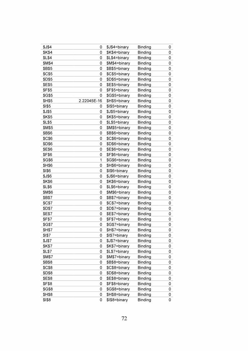
72
$J$4 0 $J$4=binary Binding 0
$K$4 0 $K$4=binary Binding 0
$L$4 0 $L$4=binary Binding 0
$M$4 0 $M$4=binary Binding 0
$B$5 0 $B$5=binary Binding 0
$C$5 0 $C$5=binary Binding 0
$D$5 0 $D$5=binary Binding 0
$E$5 0 $E$5=binary Binding 0
$F$5 0 $F$5=binary Binding 0
$G$5 0 $G$5=binary Binding 0
$H$5 2.22045E-16 $H$5=binary Binding 0
$I$5 0 $I$5=binary Binding 0
$J$5 0 $J$5=binary Binding 0
$K$5 0 $K$5=binary Binding 0
$L$5 0 $L$5=binary Binding 0
$M$5 0 $M$5=binary Binding 0
$B$6 0 $B$6=binary Binding 0
$C$6 0 $C$6=binary Binding 0
$D$6 0 $D$6=binary Binding 0
$E$6 0 $E$6=binary Binding 0
$F$6 0 $F$6=binary Binding 0
$G$6 1 $G$6=binary Binding 0
$H$6 0 $H$6=binary Binding 0
$I$6 0 $I$6=binary Binding 0
$J$6 0 $J$6=binary Binding 0
$K$6 0 $K$6=binary Binding 0
$L$6 0 $L$6=binary Binding 0
$M$6 0 $M$6=binary Binding 0
$B$7 0 $B$7=binary Binding 0
$C$7 0 $C$7=binary Binding 0
$D$7 0 $D$7=binary Binding 0
$E$7 0 $E$7=binary Binding 0
$F$7 0 $F$7=binary Binding 0
$G$7 0 $G$7=binary Binding 0
$H$7 0 $H$7=binary Binding 0
$I$7 0 $I$7=binary Binding 0
$J$7 0 $J$7=binary Binding 0
$K$7 0 $K$7=binary Binding 0
$L$7 0 $L$7=binary Binding 0
$M$7 0 $M$7=binary Binding 0
$B$8 0 $B$8=binary Binding 0
$C$8 0 $C$8=binary Binding 0
$D$8 0 $D$8=binary Binding 0
$E$8 0 $E$8=binary Binding 0
$F$8 0 $F$8=binary Binding 0
$G$8 0 $G$8=binary Binding 0
$H$8 0 $H$8=binary Binding 0
$I$8 0 $I$8=binary Binding 0
73
$J$8 1 $J$8=binary Binding 0
$K$8 0 $K$8=binary Binding 0
$L$8 0 $L$8=binary Binding 0
$M$8 0 $M$8=binary Binding 0
$B$9 0 $B$9=binary Binding 0
$C$9 0 $C$9=binary Binding 0
$D$9 0 $D$9=binary Binding 0
$E$9 0 $E$9=binary Binding 0
$F$9 0 $F$9=binary Binding 0
$G$9 0 $G$9=binary Binding 0
$H$9 0 $H$9=binary Binding 0
$I$9 0 $I$9=binary Binding 0
$J$9 0 $J$9=binary Binding 0
$K$9 2.22045E-16 $K$9=binary Binding 0
$L$9 0 $L$9=binary Binding 0
$M$9 0 $M$9=binary Binding 0
$B$10 0 $B$10=binary Binding 0
$C$10 0 $C$10=binary Binding 0
$D$10 0 $D$10=binary Binding 0
$E$10 0 $E$10=binary Binding 0
$F$10 0 $F$10=binary Binding 0
$G$10 0 $G$10=binary Binding 0
$H$10 0 $H$10=binary Binding 0
$I$10 0 $I$10=binary Binding 0
$J$10 0 $J$10=binary Binding 0
$K$10 0 $K$10=binary Binding 0
$L$10 0 $L$10=binary Binding 0
$M$10 0 $M$10=binary Binding 0
$B$11 0 $B$11=binary Binding 0
$C$11 0 $C$11=binary Binding 0
$D$11 0 $D$11=binary Binding 0
$E$11 0 $E$11=binary Binding 0
$F$11 0 $F$11=binary Binding 0
$G$11 0 $G$11=binary Binding 0
$H$11 0 $H$11=binary Binding 0
$I$11 0 $I$11=binary Binding 0
$J$11 0 $J$11=binary Binding 0
$K$11 0 $K$11=binary Binding 0
$L$11 0 $L$11=binary Binding 0
$M$11 1 $M$11=binary Binding 0
$B$12 0 $B$12=binary Binding 0
$C$12 0 $C$12=binary Binding 0
$D$12 0 $D$12=binary Binding 0
$E$12 0 $E$12=binary Binding 0
$F$12 0 $F$12=binary Binding 0
$G$12 0 $G$12=binary Binding 0
$H$12 0 $H$12=binary Binding 0
$I$12 0 $I$12=binary Binding 0
74
$J$12 0 $J$12=binary Binding 0
$K$12 0 $K$12=binary Binding 0
$L$12 0 $L$12=binary Binding 0
$M$12 2.22045E-16 $M$12=binary Binding 0
$B$13 0 $B$13=binary Binding 0
$C$13 0 $C$13=binary Binding 0
$D$13 0 $D$13=binary Binding 0
$E$13 0 $E$13=binary Binding 0
$F$13 0 $F$13=binary Binding 0
$G$13 0 $G$13=binary Binding 0
$H$13 0 $H$13=binary Binding 0
$I$13 0 $I$13=binary Binding 0
$J$13 0 $J$13=binary Binding 0
$K$13 0 $K$13=binary Binding 0
$L$13 0 $L$13=binary Binding 0
$M$13 0 $M$13=binary Binding 0
$B$14 0 $B$14=binary Binding 0
$C$14 0 $C$14=binary Binding 0
$D$14 0 $D$14=binary Binding 0
$E$14 0 $E$14=binary Binding 0
$F$14 0 $F$14=binary Binding 0
$G$14 0 $G$14=binary Binding 0
$H$14 0 $H$14=binary Binding 0
$I$14 0 $I$14=binary Binding 0
$J$14 0 $J$14=binary Binding 0
$K$14 0 $K$14=binary Binding 0
$L$14 0 $L$14=binary Binding 0
$M$14 0 $M$14=binary Binding 0
75
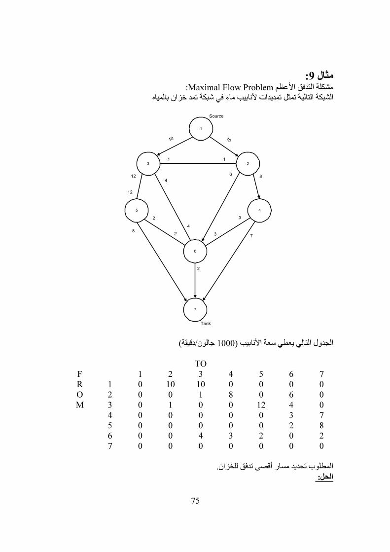
:9مثال
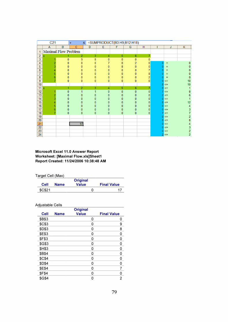
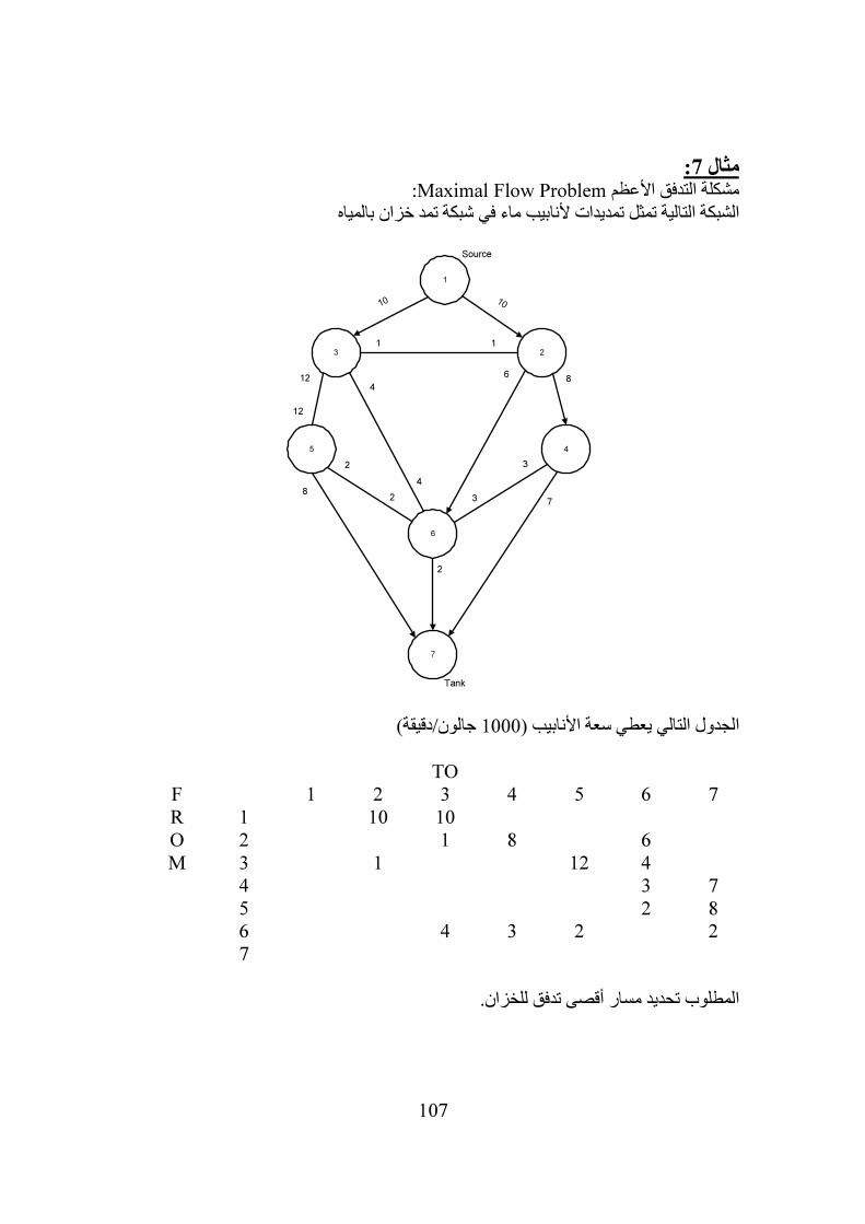
:Maximal Flow Problemمشكلة التدفق األعظم مديدات ألنابيب ماء في شبكة تمد خزان بالمياهالشبكة التالية تمثل ت
1
23
45
6
7
1010
1 1
4
4
12
2
2
68
7
3
3
2
8
12
Source
Tank
جالون/دقيقة) 1000الجدول التالي يعطي سعة األنابيب (
TO 7 6 5 4 3 2 1 F
R O M
0 0 0 0 10 10 0 1 0 6 0 8 1 0 0 2 0 4 12 0 0 1 0 3 7 3 0 0 0 0 0 4 8 2 0 0 0 0 0 5 2 0 2 3 4 0 0 6 0 0 0 0 0 0 0 7
المطلوب تحديد مسار أقصى تدفق للخزان.
الحل:
76
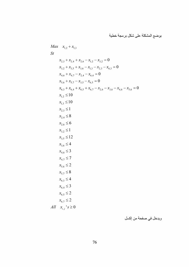
بوضع المشكلة على شكل برمجة خطية
1,2 1,3
2,3 2,4 2,6 1,2 3,2
3,2 3,5 3,6 1,3 2,3 6,3
4,6 4,7 2,4 6,4
5,6 5,7 3,5 6,5
6,3 6,4 6,5 6,7 2,6 3,6 4,6 5,6
1,2
1,3
2,3
2,4
2,6
3,2
3,5
0
0
0
0
0
10
10
1
8
6
1
12
Max x x
St
x x x x x
x x x x x x
x x x x
x x x x
x x x x x x x x
x
x
x
x
x
x
x
x
+
+ + − − =
+ + − − − =
+ − − =
+ − − =
+ + + − − − − =
≤
≤
≤
≤
≤
≤
≤
3,6
4,6
4,7
5,6
5,7
6,3
6,4
6,5
6,7
,
4
3
7
2
8
4
3
2
2
' 0i j
x
x
x
x
x
x
x
x
All x s
≤
≤
≤
≤
≤
≤
≤
≤
≤
≥
ويدخل في صفحة من إكسل
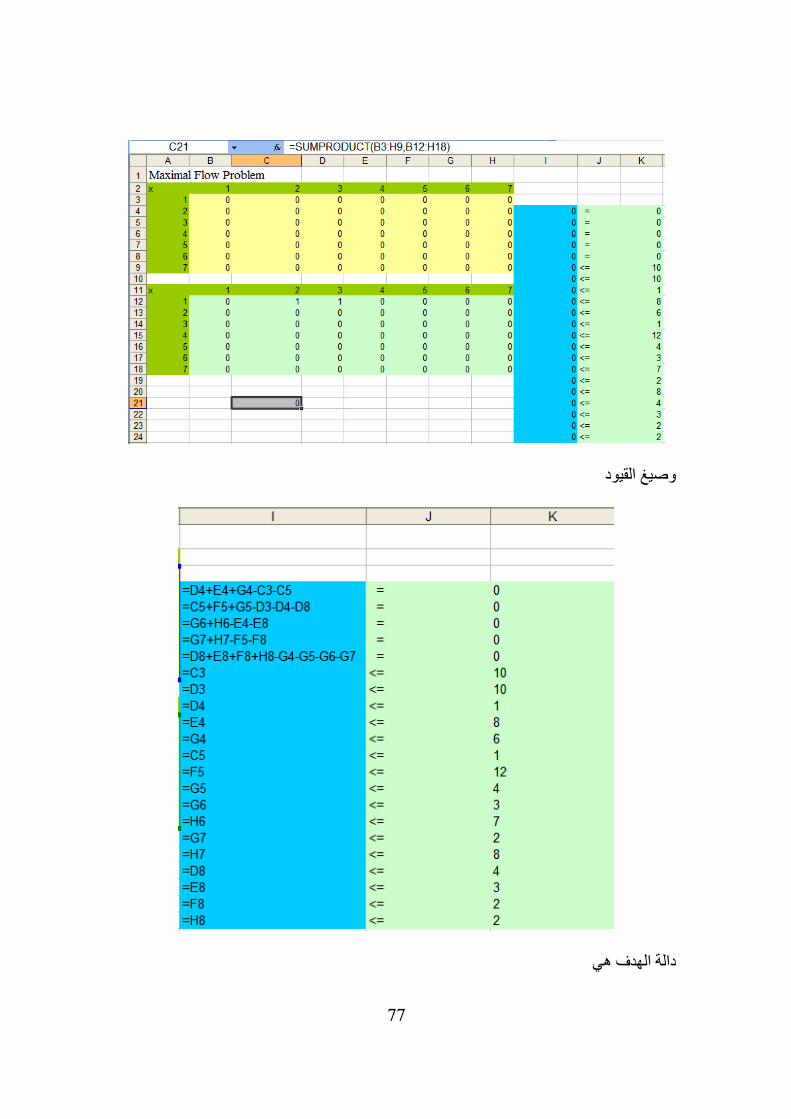
77
وصيغ القيود
دالة الهدف هي

78
Solverويدخل التالي في نافذة حوار
وينتج الحل التالي
79
Microsoft Excel 11.0 Answer Report
Worksheet: [Maximal Flow.xls]Sheet1
Report Created: 11/24/2006 10:38:48 AM
Target Cell (Max)
Cell Name Original Value Final Value
$C$21 0 17
Adjustable Cells
Cell Name Original Value Final Value
$B$3 0 0
$C$3 0 9
$D$3 0 8
$E$3 0 0
$F$3 0 0
$G$3 0 0
$H$3 0 0
$B$4 0 0
$C$4 0 0
$D$4 0 0
$E$4 0 7
$F$4 0 0
$G$4 0 2
80
$H$4 0 0
$B$5 0 0
$C$5 0 0
$D$5 0 0
$E$5 0 0
$F$5 0 8
$G$5 0 0
$H$5 0 0
$B$6 0 0
$C$6 0 0
$D$6 0 0
$E$6 0 0
$F$6 0 0
$G$6 0 0
$H$6 0 7
$B$7 0 0
$C$7 0 0
$D$7 0 0
$E$7 0 0
$F$7 0 0
$G$7 0 0
$H$7 0 8
$B$8 0 0
$C$8 0 0
$D$8 0 0
$E$8 0 0
$F$8 0 0
$G$8 0 0
$H$8 0 2
$B$9 0 0
$C$9 0 0
$D$9 0 0
$E$9 0 0
$F$9 0 0
$G$9 0 0
$H$9 0 0
Constraints
Cell Name Cell Value Formula Status Slack
$I$4 0 $I$4=$K$4 Not Binding 0
$I$5 0 $I$5=$K$5 Not Binding 0
$I$6 0 $I$6=$K$6 Not Binding 0
$I$7 0 $I$7=$K$7 Not Binding 0
$I$8 0 $I$8=$K$8 Not 0
81
Binding
$I$9 9 $I$9<=$K$9 Not Binding 1
$I$10 8 $I$10<=$K$10 Not Binding 2
$I$11 x 0 $I$11<=$K$11 Not Binding 1
$I$12 7 $I$12<=$K$12 Not Binding 1
$I$13 2 $I$13<=$K$13 Not Binding 4
$I$14 0 $I$14<=$K$14 Not Binding 1
$I$15 8 $I$15<=$K$15 Not Binding 4
$I$16 0 $I$16<=$K$16 Not Binding 4
$I$17 0 $I$17<=$K$17 Not Binding 3
$I$18 7 $I$18<=$K$18 Binding 0
$I$19 0 $I$19<=$K$19 Not Binding 2
$I$20 8 $I$20<=$K$20 Binding 0
$I$21 0 $I$21<=$K$21 Not Binding 4
$I$22 0 $I$22<=$K$22 Not Binding 3
$I$23 0 $I$23<=$K$23 Not Binding 2
$I$24 2 $I$24<=$K$24 Binding 0
82
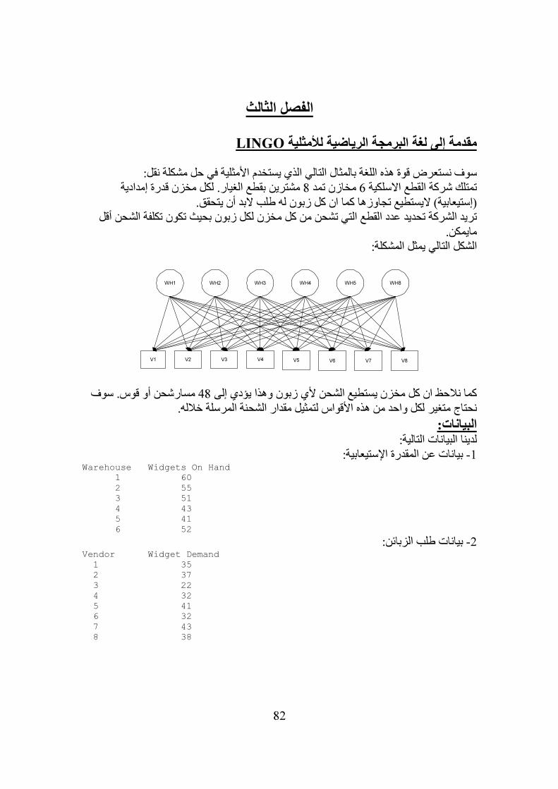
الفصل الثالث
LINGOمقدمة إلى لغة البرمجة الرياضية لألمثلية
سوف نستعرض قوة هذه اللغة بالمثال التالي الذي يستخدم األمثلية في حل مشكلة نقل:
مشترين بقطع الغيار. لكل مخزن قدرة إمدادية 8مخازن تمد 6تمتلك شركة القطع االسلكية ن كل زبون له طلب البد أن يتحقق.(إستيعابية) اليستطيع تجاوزها كما ا
تريد الشركة تحديد عدد القطع التي تشحن من كل مخزن لكل زبون بحيث تكون تكلفة الشحن أقل مايمكن.
الشكل التالي يمثل المشكلة:
WH1 WH3WH2 WH4 WH5 WH8
V1 V2 V3 V4 V5 V6 V7 V8
. سوف مسارشحن أو قوس 48كما نالحظ ان كل مخزن يستطيع الشحن ألي زبون وهذا يؤدي إلى نحتاج متغير لكل واحد من هذه األقواس لتمثيل مقدار الشحنة المرسلة خالله.
البيانات:
لدينا البيانات التالية: بيانات عن المقدرة اإلستيعابية: -1
Warehouse Widgets On Hand 1 60 2 55 3 51 4 43 5 41 6 52
بيانات طلب الزبائن: -2Vendor Widget Demand 1 35 2 37 3 22 4 32 5 41 6 32 7 43 8 38

83
تكاليف الشحن للقطعة: -3 V1 V2 V3 V4 V5 V6 V7 V8 WH1 6 2 6 7 4 2 5 9 WH2 4 9 5 3 8 5 8 2 WH3 5 2 1 9 7 4 3 3 WH4 7 6 7 3 9 2 7 1 WH5 2 3 9 5 7 2 6 5 WH6 5 5 2 2 8 1 4 3
: The Objective Functionدالة الهدف لتشكيل النموذج سوف نبدأ ببناء دالة الهدف. المطلوب تقليل تكلفة الشحن ولهذا سنستخدم المتغير
( ),x i j لكي يمثل عدد القطع التي تشحن من الخزنi إلى الزبونj لهدف تكتب علي ولهذا فإن دالة ا
الشكل:Minimize
( ) ( ) ( ) ( ) ( ) ( ) ( ) ( )
( ) ( ) ( ) ( ) ( ) ( ) ( ) ( )
( ) ( ) ( ) ( ) ( ) ( ) ( ) ( )
( ) ( ) ( ) ( ) ( ) ( ) ( ) ( )
( )
6 1,1 2 1, 2 6 1,3 7 1, 4 4 1,5 2 1,6 5 1,7 9 1,8
4 2,1 9 2, 2 5 2,3 3 2, 4 8 2,5 5 2,6 8 2,7 2 2,8
5 3,1 2 3,2 3,3 9 3, 4 7 3,5 4 3,6 3 3,7 3 3,8
7 4,1 6 4,2 7 4,3 3 4,4 9 4,5 2 4,6 7 4,7 4,8
2 5,1 3 5,
x x x x x x x x
x x x x x x x x
x x x x x x x x
x x x x x x x x
x x
+ + + + + + + +
+ + + + + + + +
+ + + + + + + +
+ + + + + + + +
+ ( ) ( ) ( ) ( ) ( ) ( ) ( )
( ) ( ) ( ) ( ) ( ) ( ) ( ) ( )
2 9 5,3 5 5, 4 7 5,5 2 5,6 6 5,7 5 5,8
5 6,1 5 6, 2 2 6,3 2 6, 4 8 6,5 6,6 4 6,7 3 6,8
x x x x x x
x x x x x x x x
+ + + + + + +
+ + + + + + +
زبائن فكيف سوف تكون لو كان 8مخازن و 6كما نشاهد فإن دالة الهدف معقدة جدا وذلك فقط لـ
لدينا عشرات بل مئات المخازن وآالف من الزبائن؟ كما أن إدخال مثل هذه الصيغة في برنامج ون بالتأكيد معرضا للخطأ.حاسب سيك
الصيغة السابقة يمكن وضعها على شكل الصيغة الرياضية التالية:
( )6 8
1 1
,
ij
i j
Mimize c x i j= =
∑∑
حيث ijc تكلفة شحن القطعة الواحدة من مخزنi إلى الزبونj .
تصر سهل الكتابة والفهم تسمح بتمثيل دالة الهدف بشكل مخ LINGOوبالمثل فإن لغة النمذجة كالتالي:
MIN = @SUM(LINKS(I,J): COST(I,J)*VOLUME(I,J));
تكلفة COST(I,J)و jإلى الزبون iيمثل عدد القطع التي تشحن من المخزن VOLUME(I,J)حيث LINKS(I,J)و الجمع يكون على كل الروابط jإلى الزبون iشحن القطعة الواحدة من مخزن
LINGOول التالي مقارنة بين الصيغة الرياضية ولغة بينهما. الجد

84
Math Notation LINGO Syntax
Minimize MIN =
6 8
1 1i j= =∑ ∑
@SUM(LINKS(I,J): )
ijc COST(I,J)
( ),x i j VOLUME(I,J)
:onstraintsCالقيود
للنموذج. مجموعة القيود Constraintsبعد صياغتنا لدالة الهدف خطوتنا التالية صياغة القيود األولى تضمن إستالم كل زبون لعدد القطع التي طلبها وسوف نسمي هذه القيود قيود الطلب
Demand Constraints مجموعة القيود التالية والتي نسميها قيود السعةCapacity Constraints .تضمن عدم شحن قطع من مخزن تزيد عن المقدار الذى يمتلكة
بدأ بقيد الطلب للزبون األول فإننا نحتاج إلى جمع كل الشحنات من جميع المخازن وجعلها مساوية قطعة أي 35لطلب الزبون األول
( ) ( ) ( ) ( ) ( ) ( )1,1 2,1 3,1 4,1 5,1 6,1 35x x x x x x+ + + + + = وهكذا لبقية الزبائن
( ) ( ) ( ) ( ) ( ) ( )1, 2 2,2 3,2 4, 2 5,2 6,2 37x x x x x x+ + + + + =
( ) ( ) ( ) ( ) ( ) ( )1,3 2,3 3,3 4,3 5,3 6,3 22x x x x x x+ + + + + =
( ) ( ) ( ) ( ) ( ) ( )1, 4 2,4 3,4 4, 4 5,4 6,4 32x x x x x x+ + + + + =
( ) ( ) ( ) ( ) ( ) ( )1,5 2,5 3,5 4,5 5,5 6,5 41x x x x x x+ + + + + =
( ) ( ) ( ) ( ) ( ) ( )1,6 2,6 3,6 4,6 5,6 6,6 32x x x x x x+ + + + + =
( ) ( ) ( ) ( ) ( ) ( )1,7 2,7 3,7 4,7 5,7 6,7 43x x x x x x+ + + + + =
( ) ( ) ( ) ( ) ( ) ( )1,8 2,8 3,8 4,8 5,8 6,8 38x x x x x x+ + + + + = وهنا ينطبق نفس التعليق الذي تبع صياغة دالة الهدف.
كالتالي:قيود الطلب تكتب بصيغة رياضية بسيطة
( )6
1
, , 1, 2,...,8j
i
x i j d j=
= =∑
حيث j
d عدد القطع المطلوبة من الزبونj . تكتب قيود الطلب LINGOوبلغة النمذجة
@FOR(VENDORS(J): @SUM(WAREHOUSES(I): VOLUME(I,J)) = DEMAND(J));
السابقة ( بل يمكن أن تمثل مجموعة من تمثل مجموعة القيود LINGOهذه العبارة بلغة النمذجة فإن مجموع VENDORSآالف الزبائن ومئآت المخازن ايضا). العبارة السابقة تدل على انه لكل الزبائن
إلى ذلك الزبون يجب أن تساوي WAREHOUSESمن كل مخزن VOLUMEالقطع التي تشحن لصيغة الرياضية. الجدول التالي ذلك الزبون. الحظ مدى تشابه هذه العبارة مع ا DEMANDلطلب
يعطى مقارنة بينهما:

85
Math Notation LINGO Syntax
1,2,...,8j = @FOR(VENDORS(J): )
6
1i=∑
@SUM(WAREHOUSES(I): )
( ),x i j VOLUME(I,J)
= =
jd DEMAND(J)
سوف نصيغ اآلن قيود السعة والتي تكتب بصيغة الرياضيات
( )8
1
, , 1, 2,...,6j
j
x i j p i=
≤ =∑
حيث j
p هي سعة المخزنj متراجحات ) 8.(الحظ ان هذه الصيغة الرياضية تمثل مجموعة من تكتب قيود السعة LINGOوبلغة النمذجة
@FOR( WAREHOUSES( I): @SUM( VENDORS( J): VOLUME( I, J)) <= CAPACITY( I));
يجب اال تزيد VENDORSللزبائن VOLUMEفإن مجموع القطع المشحونة WAREHOUSESأي لكل مخزن ذلك المخزن. CAPACITYعن سعة
كالتالي: LINGOاآلن نكتب النموذج كامال بلغة النمذجة MODEL: MIN = @SUM( LINKS( I, J): COST( I, J) * VOLUME( I, J)); @FOR( VENDORS( J): @SUM( WAREHOUSES( I): VOLUME( I, J)) = DEMAND( J)); @FOR( WAREHOUSES( I): @SUM( VENDORS( J): VOLUME( I, J)) <= CAPACITY( I)); END
Model: WIDGETSلنسمي هذا وقسم البيانات Sets Sectionا يسمى بقسم المجموعات إلكمال النموذج يجب ان نعرف البيانات فيم
Data Section :والتى نشرحها بالتفصيل كالتالي
تعريف المجموعات:عند قيامنا بالنمذجة في الحياة العملية فإننا نقابل مجموعة او اكثر من األشياء التي لها عالقة ببعضها
ين الخ. في الغالب إذا طبق قيد على عضو من البعض مثل الزبائن ، المصانع ، السيارات ، الموظفالمجموعة فإن هذا القيد يطبق بالتمام على األعضاء اآلخرين في المجموعة. هذا المبدأ هو من
إذ يعطى المقدرة على تعريف مجموعات من األشياء المترابطة في LINGOأساسيات لغة النمذجة قسم المجموعات.
توضع في سطر منفردة وينتهي SETSالتي هي Keywordس قسم المجموعات يبدأ بكلمة األسا LINGOايضا على سطر منفرد. بعد تعريف أعضاء المجموعة فإن ENDSETSالقسم بكلمة األساس
) والتي تطبق بعض FOR@( مثل Set Looping Functionsيمتلك مجموعة من دوال الدورة واحدة فقط. العمليات على جميع اعضاء المجموعة بإستخدام عبارة
في حالة نموذجنا فإننا قمنا بتكوين ثالثة مجموعات هي: Warehousesالمخازن -1

86
Vendorsالزبائن -2 Shipping Arcsتوصيالت او أقواس الشحن من كل مخزن إلى كل زبون -3
تعرف هذه المجموعات كالتالي: LINGOوبلغة النمذجة SETS: WAREHOUSES / WH1 WH2 WH3 WH4 WH5 WH6/: CAPACITY; VENDORS / V1 V2 V3 V4 V5 V6 V7 V8/ : DEMAND; LINKS( WAREHOUSES, VENDORS): COST, VOLUME;
ENDSETS
,WH1أعضائها هم WAREHOUSESيقول ان المجموعة SETSالسطر األول بعد كلمة األساس WH2,…,WH6 كل منها له صفةAttribute تسمىCAPACITY لسطر التالي يعرف مجموعة الزبائن . اVENDORS والتي أعضائهاV1,V2,…,V8 والتي لكل واحد منها الصفةDEMAND المجموعة األخيرة .التابعة لها. VOLUMEو COSTتوصيلة او خط شحن كل توصيلة لها صفات 48تمثل LINKSالمسماة
ة والمجاميع السابقة فبوضع بين المجموعة هذ Syntaxالحظ اإلختالف في التركيب اللغوي LINKS( WAREHOUSES, VENDORS) فإننا نخبرLINGO أن مجموعةLINKS تستنبط من
من األزواج المرتبة 48يولد LINGOوبالتالي فإن VENDORSو WAREHOUSESالمجموعتين WAREHOUSES, VENDORS) ( ويجعلها أعضاء في المجموعةLINKS .
إدخال البيانات:
البيانات في قسم البيانات كالتالي:تدخل DATA: CAPACITY = 60 55 51 43 41 52; DEMAND = 35 37 22 32 41 32 43 38; COST = 6 2 6 7 4 2 5 9 4 9 5 3 8 5 8 2 5 2 1 9 7 4 3 3 7 6 7 3 9 2 7 1 2 3 9 5 7 2 6 5 5 5 2 2 8 1 4 3; ENDDATA
على سطر ENDDATAعلى سطر منفرد وينتهي بكلمة األساس DATAيبدأ قسم البيانات بكلمة األساس
VENDORSللمجموعة DEMANDو WAREHOUSESللمجموعة CAPACITYمنفرد ايضا. كل من الصفات ألبعاد يتم قرائتها بواسطة ثنائية ا LINKSللمجموعة COSTاسند لها قيم بشكل مباشر. الصفة
LINGO :بزيادة الدورة الخارجية أسرع من الدورة الداخلية أي يقرأ القيم على الترتيب التالي COST(WH1,V1), COST(WH1,V2), COST(WH1,V3),…,COST(WH1,V8), COST(WH2,V1), COST(WH2,V2), COST(WH2,V3),…,COST(WH2,V8), … COST(WH6,V1), COST(WH6,V2 ), COST(WH6,V3),…,COST(WH6,V8)
الحظ اننا هنا أدخلنا البيانات بشكل مباشر ولكن يمكننا قرائتها من ملف او إستيرادها من صفحة نشر وسوف نتطرق لهذا الحقا. EXCELمثل
النموذج بشكله الكامل:MODEL: ! A 6 Warehouse 8 Vendor Transportation Problem;
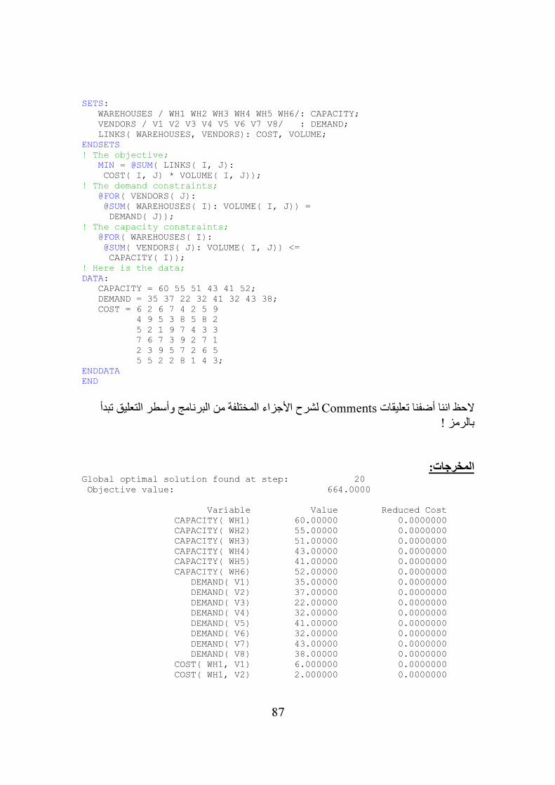
87
SETS: WAREHOUSES / WH1 WH2 WH3 WH4 WH5 WH6/: CAPACITY; VENDORS / V1 V2 V3 V4 V5 V6 V7 V8/ : DEMAND; LINKS( WAREHOUSES, VENDORS): COST, VOLUME; ENDSETS ! The objective; MIN = @SUM( LINKS( I, J): COST( I, J) * VOLUME( I, J)); ! The demand constraints; @FOR( VENDORS( J): @SUM( WAREHOUSES( I): VOLUME( I, J)) = DEMAND( J)); ! The capacity constraints; @FOR( WAREHOUSES( I): @SUM( VENDORS( J): VOLUME( I, J)) <= CAPACITY( I)); ! Here is the data; DATA: CAPACITY = 60 55 51 43 41 52; DEMAND = 35 37 22 32 41 32 43 38; COST = 6 2 6 7 4 2 5 9 4 9 5 3 8 5 8 2 5 2 1 9 7 4 3 3 7 6 7 3 9 2 7 1 2 3 9 5 7 2 6 5 5 5 2 2 8 1 4 3; ENDDATA END
من البرنامج وأسطر التعليق تبدأ لشرح األجزاء المختلفة Commentsالحظ اننا أضفنا تعليقات
بالرمز !
المخرجات:Global optimal solution found at step: 20 Objective value: 664.0000 Variable Value Reduced Cost CAPACITY( WH1) 60.00000 0.0000000 CAPACITY( WH2) 55.00000 0.0000000 CAPACITY( WH3) 51.00000 0.0000000 CAPACITY( WH4) 43.00000 0.0000000 CAPACITY( WH5) 41.00000 0.0000000 CAPACITY( WH6) 52.00000 0.0000000 DEMAND( V1) 35.00000 0.0000000 DEMAND( V2) 37.00000 0.0000000 DEMAND( V3) 22.00000 0.0000000 DEMAND( V4) 32.00000 0.0000000 DEMAND( V5) 41.00000 0.0000000 DEMAND( V6) 32.00000 0.0000000 DEMAND( V7) 43.00000 0.0000000 DEMAND( V8) 38.00000 0.0000000 COST( WH1, V1) 6.000000 0.0000000 COST( WH1, V2) 2.000000 0.0000000
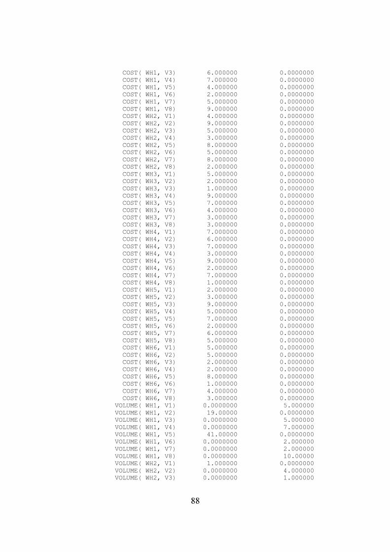
88
COST( WH1, V3) 6.000000 0.0000000 COST( WH1, V4) 7.000000 0.0000000 COST( WH1, V5) 4.000000 0.0000000 COST( WH1, V6) 2.000000 0.0000000 COST( WH1, V7) 5.000000 0.0000000 COST( WH1, V8) 9.000000 0.0000000 COST( WH2, V1) 4.000000 0.0000000 COST( WH2, V2) 9.000000 0.0000000 COST( WH2, V3) 5.000000 0.0000000 COST( WH2, V4) 3.000000 0.0000000 COST( WH2, V5) 8.000000 0.0000000 COST( WH2, V6) 5.000000 0.0000000 COST( WH2, V7) 8.000000 0.0000000 COST( WH2, V8) 2.000000 0.0000000 COST( WH3, V1) 5.000000 0.0000000 COST( WH3, V2) 2.000000 0.0000000 COST( WH3, V3) 1.000000 0.0000000 COST( WH3, V4) 9.000000 0.0000000 COST( WH3, V5) 7.000000 0.0000000 COST( WH3, V6) 4.000000 0.0000000 COST( WH3, V7) 3.000000 0.0000000 COST( WH3, V8) 3.000000 0.0000000 COST( WH4, V1) 7.000000 0.0000000 COST( WH4, V2) 6.000000 0.0000000 COST( WH4, V3) 7.000000 0.0000000 COST( WH4, V4) 3.000000 0.0000000 COST( WH4, V5) 9.000000 0.0000000 COST( WH4, V6) 2.000000 0.0000000 COST( WH4, V7) 7.000000 0.0000000 COST( WH4, V8) 1.000000 0.0000000 COST( WH5, V1) 2.000000 0.0000000 COST( WH5, V2) 3.000000 0.0000000 COST( WH5, V3) 9.000000 0.0000000 COST( WH5, V4) 5.000000 0.0000000 COST( WH5, V5) 7.000000 0.0000000 COST( WH5, V6) 2.000000 0.0000000 COST( WH5, V7) 6.000000 0.0000000 COST( WH5, V8) 5.000000 0.0000000 COST( WH6, V1) 5.000000 0.0000000 COST( WH6, V2) 5.000000 0.0000000 COST( WH6, V3) 2.000000 0.0000000 COST( WH6, V4) 2.000000 0.0000000 COST( WH6, V5) 8.000000 0.0000000 COST( WH6, V6) 1.000000 0.0000000 COST( WH6, V7) 4.000000 0.0000000 COST( WH6, V8) 3.000000 0.0000000 VOLUME( WH1, V1) 0.0000000 5.000000 VOLUME( WH1, V2) 19.00000 0.0000000 VOLUME( WH1, V3) 0.0000000 5.000000 VOLUME( WH1, V4) 0.0000000 7.000000 VOLUME( WH1, V5) 41.00000 0.0000000 VOLUME( WH1, V6) 0.0000000 2.000000 VOLUME( WH1, V7) 0.0000000 2.000000 VOLUME( WH1, V8) 0.0000000 10.00000 VOLUME( WH2, V1) 1.000000 0.0000000 VOLUME( WH2, V2) 0.0000000 4.000000 VOLUME( WH2, V3) 0.0000000 1.000000
89
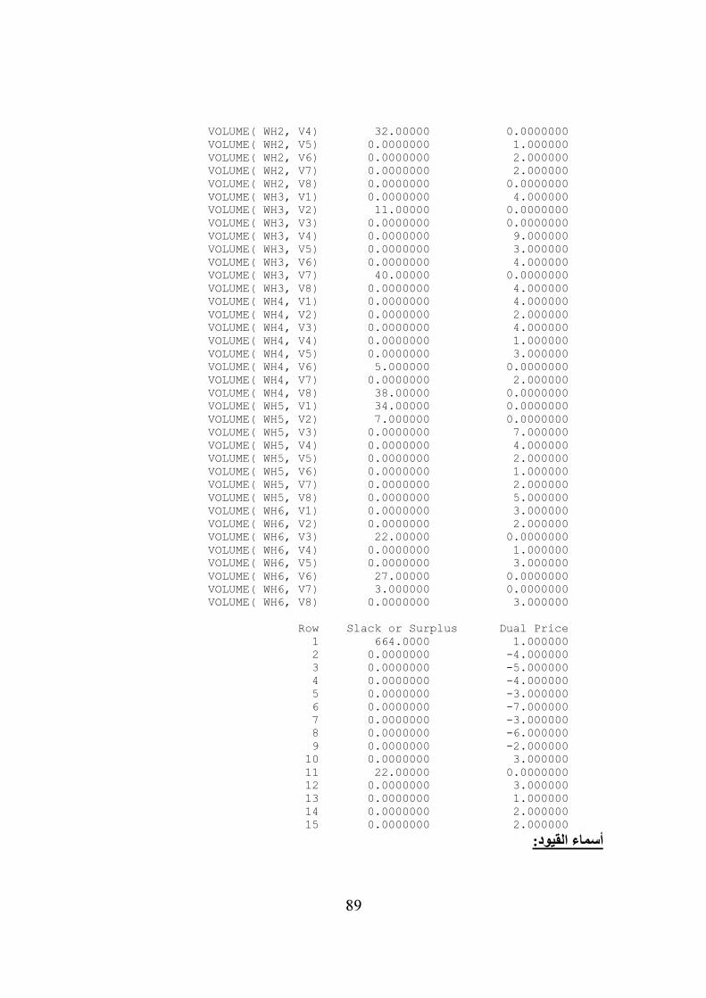
VOLUME( WH2, V4) 32.00000 0.0000000 VOLUME( WH2, V5) 0.0000000 1.000000 VOLUME( WH2, V6) 0.0000000 2.000000 VOLUME( WH2, V7) 0.0000000 2.000000 VOLUME( WH2, V8) 0.0000000 0.0000000 VOLUME( WH3, V1) 0.0000000 4.000000 VOLUME( WH3, V2) 11.00000 0.0000000 VOLUME( WH3, V3) 0.0000000 0.0000000 VOLUME( WH3, V4) 0.0000000 9.000000 VOLUME( WH3, V5) 0.0000000 3.000000 VOLUME( WH3, V6) 0.0000000 4.000000 VOLUME( WH3, V7) 40.00000 0.0000000 VOLUME( WH3, V8) 0.0000000 4.000000 VOLUME( WH4, V1) 0.0000000 4.000000 VOLUME( WH4, V2) 0.0000000 2.000000 VOLUME( WH4, V3) 0.0000000 4.000000 VOLUME( WH4, V4) 0.0000000 1.000000 VOLUME( WH4, V5) 0.0000000 3.000000 VOLUME( WH4, V6) 5.000000 0.0000000 VOLUME( WH4, V7) 0.0000000 2.000000 VOLUME( WH4, V8) 38.00000 0.0000000 VOLUME( WH5, V1) 34.00000 0.0000000 VOLUME( WH5, V2) 7.000000 0.0000000 VOLUME( WH5, V3) 0.0000000 7.000000 VOLUME( WH5, V4) 0.0000000 4.000000 VOLUME( WH5, V5) 0.0000000 2.000000 VOLUME( WH5, V6) 0.0000000 1.000000 VOLUME( WH5, V7) 0.0000000 2.000000 VOLUME( WH5, V8) 0.0000000 5.000000 VOLUME( WH6, V1) 0.0000000 3.000000 VOLUME( WH6, V2) 0.0000000 2.000000 VOLUME( WH6, V3) 22.00000 0.0000000 VOLUME( WH6, V4) 0.0000000 1.000000 VOLUME( WH6, V5) 0.0000000 3.000000 VOLUME( WH6, V6) 27.00000 0.0000000 VOLUME( WH6, V7) 3.000000 0.0000000 VOLUME( WH6, V8) 0.0000000 3.000000 Row Slack or Surplus Dual Price 1 664.0000 1.000000 2 0.0000000 -4.000000 3 0.0000000 -5.000000 4 0.0000000 -4.000000 5 0.0000000 -3.000000 6 0.0000000 -7.000000 7 0.0000000 -3.000000 8 0.0000000 -6.000000 9 0.0000000 -2.000000 10 0.0000000 3.000000 11 22.00000 0.0000000 12 0.0000000 3.000000 13 0.0000000 1.000000 14 0.0000000 2.000000 15 0.0000000 2.000000
أسماء القيود:
90
المقدرة على تسمية القيود وهذا يعطى الميزات التالية، أوال تستخدم أسماء القيود LINGOيوفر لنا في تقرير الحل وهذا يساعد على سهولة تفسير النتائج، ثانيا الكثير من رسائل األخطاء تعطي القيود
طاء سيكون صعبا جدا. مالحظة: تسمية بأسمائها فإذا لم يكن للقيود أسماء فإن تعقب وإيجاد هذه األخويعطيها أسماء من المؤشر By Defaultيسمي القيود ذاتيا LINGOالقيود غير إلزامية إذ أن
الداخلي للقيود وقد يكون هذا اإلسم بشكل اليدل إطالقا عن القيد مما يجعل تفسير رسائل األخطاء سماء مناسبة تدل بشكل ما على كل أنواع القيود أكثر غموضا ولهذا فإننا نحث المنمذج على إستخدام أ
المستخدمة في النموذج.تسمية القيود سهل جدا إذ كل ما يتطلب هو إعطاء إسم له معنى في أول القيد محاط بأقواس مربعة [
[A –Z]إذ يجب أن تبدأ بحرف أو أكثر من الحروف LINGO] األسماء يجب أن تتبع قواعد لغة رمز. 32واليزيد عن [ _ ]أو [9 – 0]رقاما من ويمكن ان تحوى ا
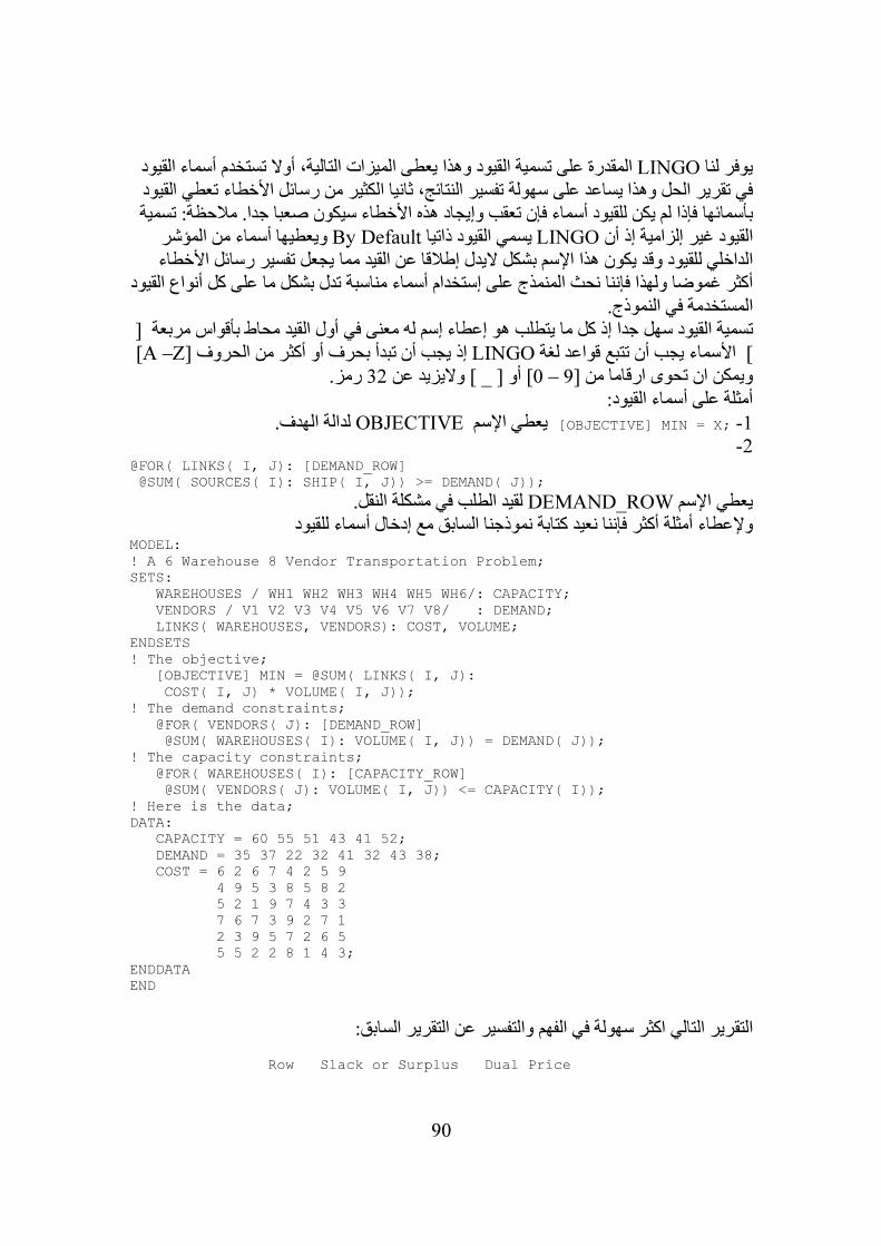
أمثلة على أسماء القيود:1- [OBJECTIVE] MIN = X; يعطي اإلسمOBJECTIVE .لدالة الهدف 2-
@FOR( LINKS( I, J): [DEMAND_ROW] @SUM( SOURCES( I): SHIP( I, J)) >= DEMAND( J));
النقل. لقيد الطلب في مشكلة DEMAND_ROWيعطي اإلسم وإلعطاء أمثلة أكثر فإننا نعيد كتابة نموذجنا السابق مع إدخال أسماء للقيود
MODEL: ! A 6 Warehouse 8 Vendor Transportation Problem; SETS: WAREHOUSES / WH1 WH2 WH3 WH4 WH5 WH6/: CAPACITY; VENDORS / V1 V2 V3 V4 V5 V6 V7 V8/ : DEMAND; LINKS( WAREHOUSES, VENDORS): COST, VOLUME; ENDSETS ! The objective; [OBJECTIVE] MIN = @SUM( LINKS( I, J): COST( I, J) * VOLUME( I, J)); ! The demand constraints; @FOR( VENDORS( J): [DEMAND_ROW] @SUM( WAREHOUSES( I): VOLUME( I, J)) = DEMAND( J)); ! The capacity constraints; @FOR( WAREHOUSES( I): [CAPACITY_ROW] @SUM( VENDORS( J): VOLUME( I, J)) <= CAPACITY( I)); ! Here is the data; DATA: CAPACITY = 60 55 51 43 41 52; DEMAND = 35 37 22 32 41 32 43 38; COST = 6 2 6 7 4 2 5 9 4 9 5 3 8 5 8 2 5 2 1 9 7 4 3 3 7 6 7 3 9 2 7 1 2 3 9 5 7 2 6 5 5 5 2 2 8 1 4 3; ENDDATA END
التقرير التالي اكثر سهولة في الفهم والتفسير عن التقرير السابق:
Row Slack or Surplus Dual Price
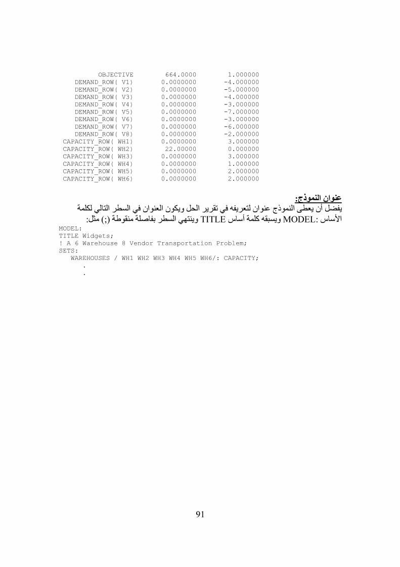
91
OBJECTIVE 664.0000 1.000000 DEMAND_ROW( V1) 0.0000000 -4.000000 DEMAND_ROW( V2) 0.0000000 -5.000000 DEMAND_ROW( V3) 0.0000000 -4.000000 DEMAND_ROW( V4) 0.0000000 -3.000000 DEMAND_ROW( V5) 0.0000000 -7.000000 DEMAND_ROW( V6) 0.0000000 -3.000000 DEMAND_ROW( V7) 0.0000000 -6.000000 DEMAND_ROW( V8) 0.0000000 -2.000000 CAPACITY_ROW( WH1) 0.0000000 3.000000 CAPACITY_ROW( WH2) 22.00000 0.000000 CAPACITY_ROW( WH3) 0.0000000 3.000000 CAPACITY_ROW( WH4) 0.0000000 1.000000 CAPACITY_ROW( WH5) 0.0000000 2.000000 CAPACITY_ROW( WH6) 0.0000000 2.000000
عنوان النموذج:
يفضل أن يعطى النموذج عنوان لتعريفه في تقرير الحل ويكون العنوان في السطر التالي لكلمة مثل: (;)وينتهي السطر بفاصلة منقوطة TITLEويسبقه كلمة أساس :MODELاألساس
MODEL: TITLE Widgets; ! A 6 Warehouse 8 Vendor Transportation Problem; SETS: WAREHOUSES / WH1 WH2 WH3 WH4 WH5 WH6/: CAPACITY; . .
92
الفصل الرابع
: LINGOأمثلة وحاالت دراسة على لغة النمذجة
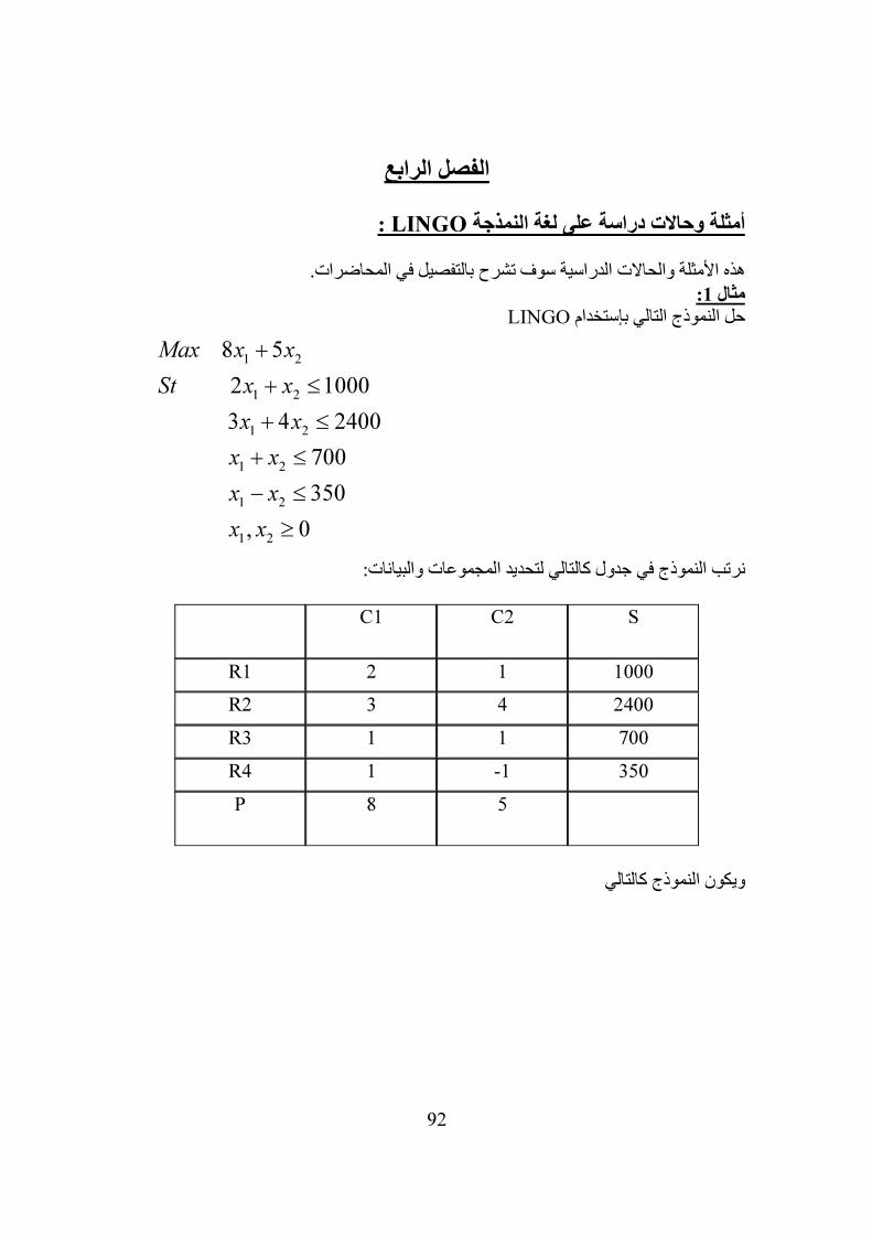
هذه األمثلة والحاالت الدراسية سوف تشرح بالتفصيل في المحاضرات.
:1مثال LINGOحل النموذج التالي بإستخدام
لتحديد المجموعات والبيانات:نرتب النموذج في جدول كالتالي
C1 C2 S
R1 2 1 1000
R2 3 4 2400
R3 1 1 700
R4 1 -1 350
P 8 5
ويكون النموذج كالتالي
1 2
1 2
1 2
1 2
1 2
1 2
8 5
2 1000
3 4 2400
700
350
, 0
Max x x
St x x
x x
x x
x x
x x
+
+ ≤
+ ≤
+ ≤
− ≤
≥
93
:التقريرGlobal optimal solution found at iteration: 3 Objective value: 4360.000 Variable Value Reduced Cost S( R1) 1000.000 0.000000 S( R2) 2400.000 0.000000 S( R3) 700.0000 0.000000 S( R4) 350.0000 0.000000 P( C1) 8.000000 0.000000 P( C2) 5.000000 0.000000 DV( C1) 320.0000 0.000000 DV( C2) 360.0000 0.000000 COEF( R1, C1) 2.000000 0.000000 COEF( R1, C2) 1.000000 0.000000 COEF( R2, C1) 3.000000 0.000000 COEF( R2, C2) 4.000000 0.000000 COEF( R3, C1) 1.000000 0.000000 COEF( R3, C2) 1.000000 0.000000 COEF( R4, C1) 1.000000 0.000000 COEF( R4, C2) -1.000000 0.000000 Row Slack or Surplus Dual Price 1 4360.000 1.000000 2 0.000000 3.40000 3 0.000000 0.4000000 4 20.00000 0.000000 5 390.0000 0.000000
94
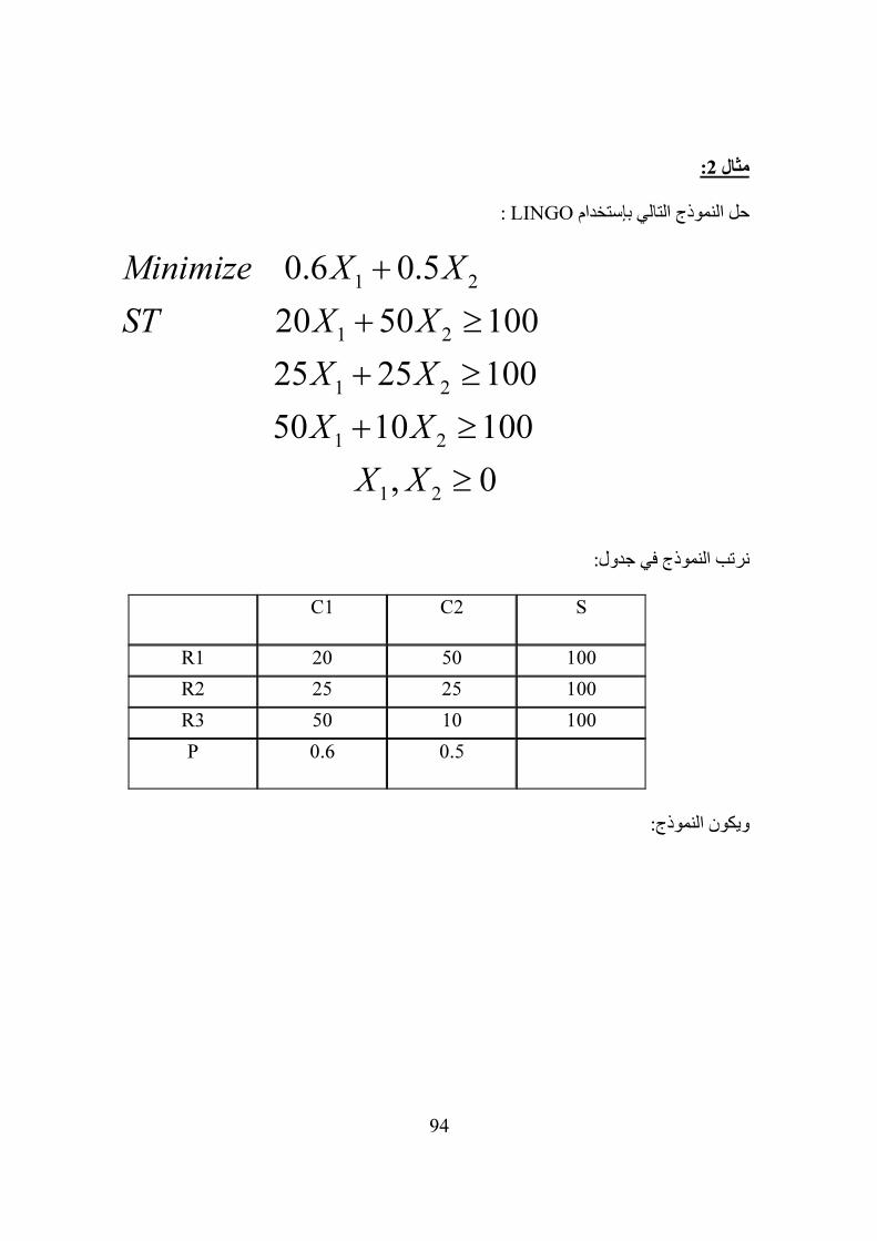
:2مثال
: LINGOحل النموذج التالي بإستخدام
نرتب النموذج في جدول:
C1 C2 S
R1 20 50 100
R2 25 25 100
R3 50 10 100
P 0.6 0.5
ويكون النموذج:
1 2
1 2
1 2
1 2
1 2
0.6 0.5
20 50 100
25 25 100
50 10 100
, 0
Minimize X X
ST X X
X X
X X
X X
+
+ ≥
+ ≥
+ ≥
≥
95
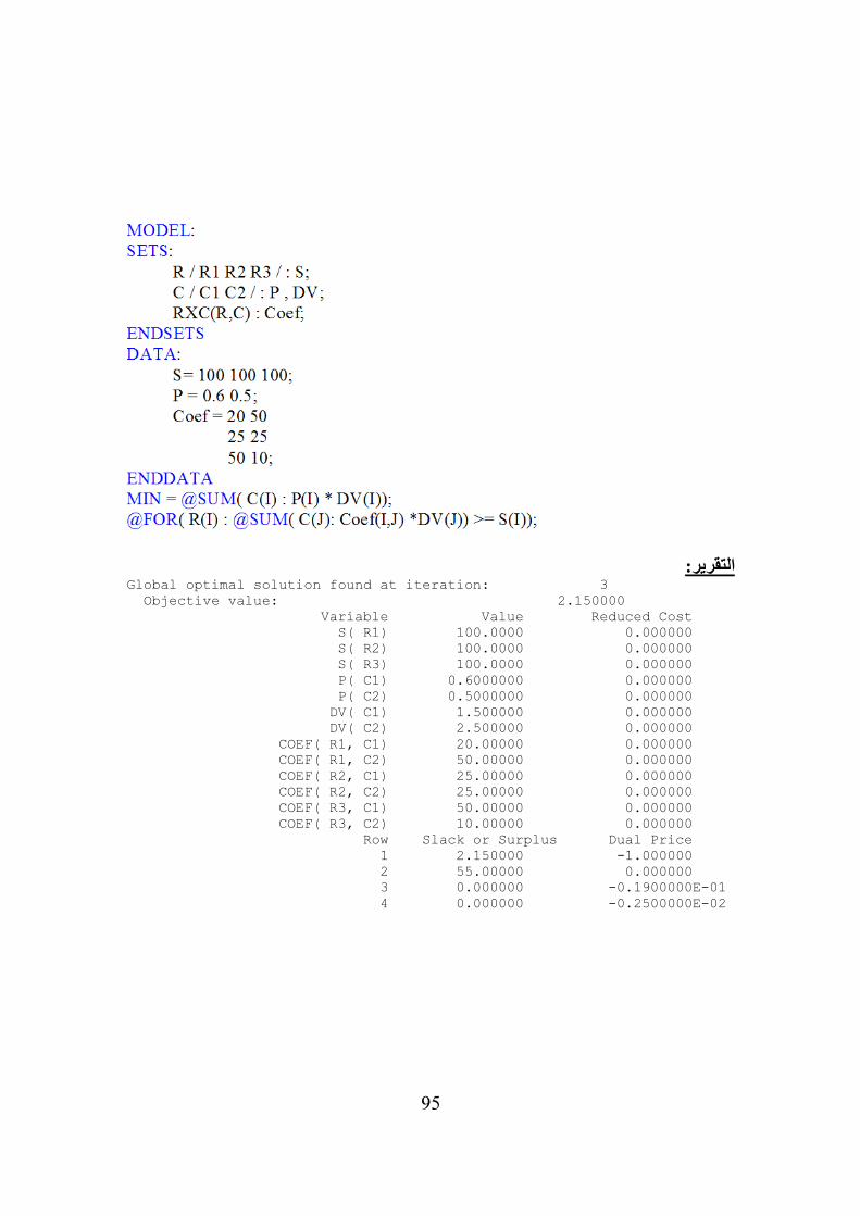
التقرير:Global optimal solution found at iteration: 3 Objective value: 2.150000 Variable Value Reduced Cost S( R1) 100.0000 0.000000 S( R2) 100.0000 0.000000 S( R3) 100.0000 0.000000 P( C1) 0.6000000 0.000000 P( C2) 0.5000000 0.000000 DV( C1) 1.500000 0.000000 DV( C2) 2.500000 0.000000 COEF( R1, C1) 20.00000 0.000000 COEF( R1, C2) 50.00000 0.000000 COEF( R2, C1) 25.00000 0.000000 COEF( R2, C2) 25.00000 0.000000 COEF( R3, C1) 50.00000 0.000000 COEF( R3, C2) 10.00000 0.000000 Row Slack or Surplus Dual Price 1 2.150000 -1.000000 2 55.00000 0.000000 3 0.000000 -0.1900000E-01 4 0.000000 -0.2500000E-02
96
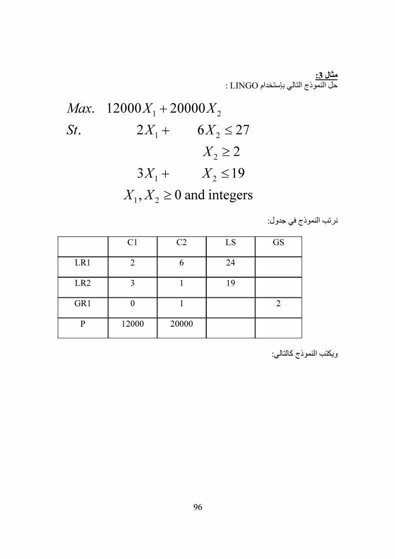
:3مثال : LINGOحل النموذج التالي بإستخدام
نرتب النموذج في جدول:
C1 C2 LS GS
LR1 2 6 24
LR2 3 1 19
GR1 0 1 2
P 12000 20000
ويكتب النموذج كالتالي:
1 2
1 2
2
1 2
1 2
. 12000 20000
. 2 6 27
2
3 19
, 0 and integers
Max X X
St X X
X
X X
X X
+
+ ≤
≥
+ ≤
≥
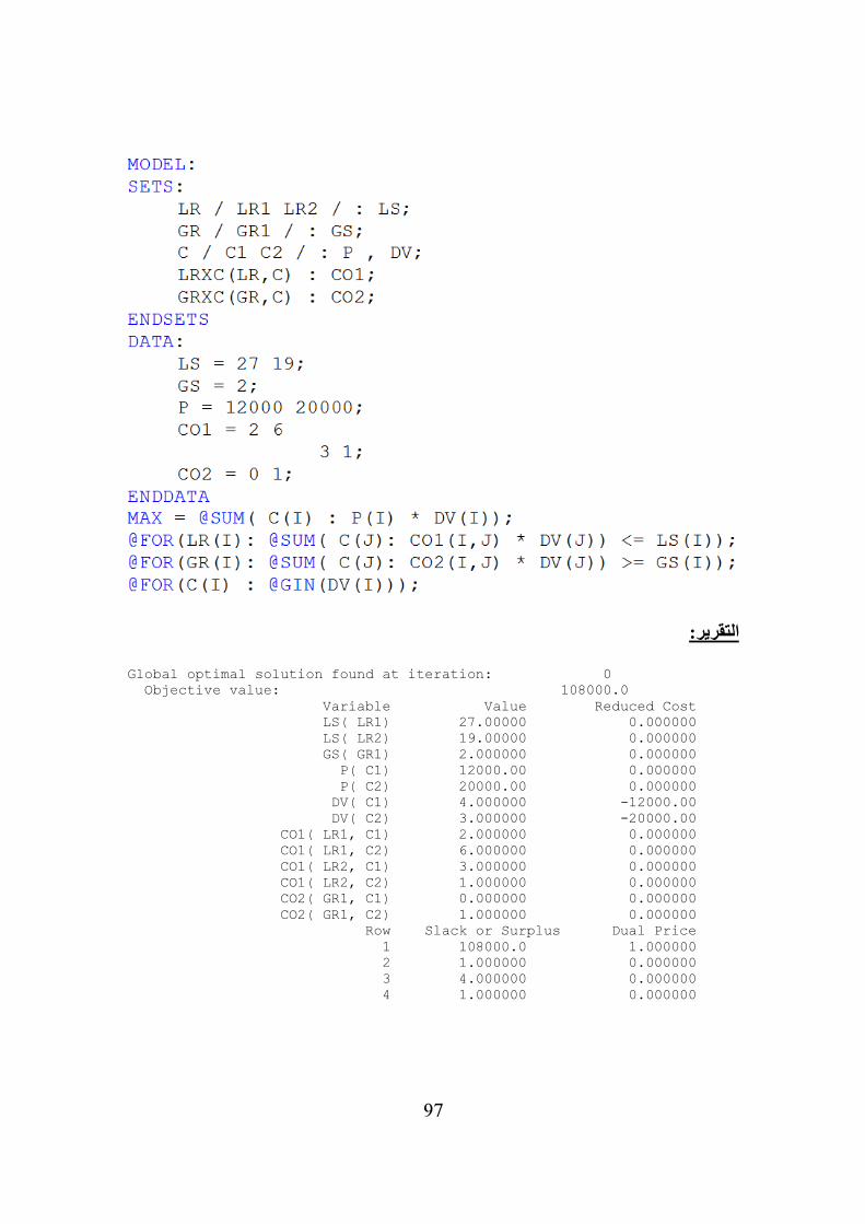
97
التقرير:
Global optimal solution found at iteration: 0 Objective value: 108000.0 Variable Value Reduced Cost LS( LR1) 27.00000 0.000000 LS( LR2) 19.00000 0.000000 GS( GR1) 2.000000 0.000000 P( C1) 12000.00 0.000000 P( C2) 20000.00 0.000000 DV( C1) 4.000000 -12000.00 DV( C2) 3.000000 -20000.00 CO1( LR1, C1) 2.000000 0.000000 CO1( LR1, C2) 6.000000 0.000000 CO1( LR2, C1) 3.000000 0.000000 CO1( LR2, C2) 1.000000 0.000000 CO2( GR1, C1) 0.000000 0.000000 CO2( GR1, C2) 1.000000 0.000000 Row Slack or Surplus Dual Price 1 108000.0 1.000000 2 1.000000 0.000000 3 4.000000 0.000000 4 1.000000 0.000000
98
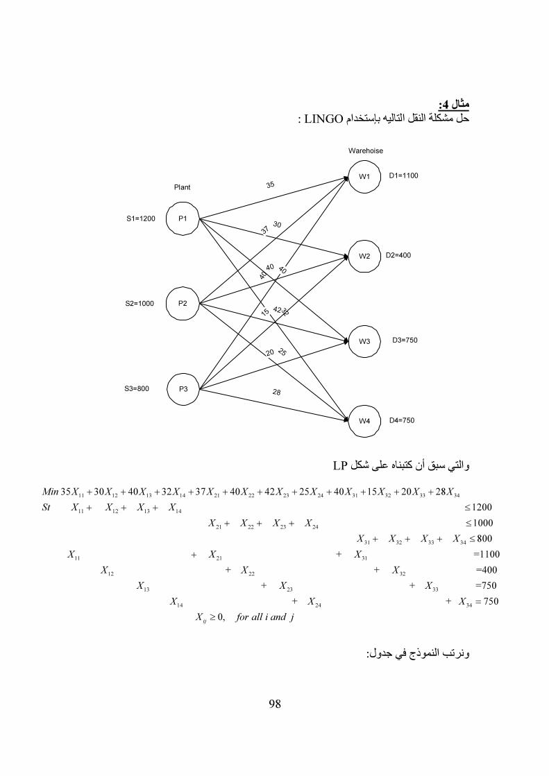
:4مثال : LINGOة النقل التاليه بإستخدام حل مشكل
LPي سبق أن كتبناه على شكل توال
ونرتب النموذج في جدول:
P1
P2
P3
W1
W2
W3
W4
35
30
32
37
40
42
25
40
15
20
28
Plant
Warehoise
S1=1200
S2=1000
S3=800
D1=1100
D2=400
D3=750
D4=750
40
11 12 13 14 21 22 23 24 31 32 33 34
11 12 13 14
35 30 40 32 37 40 42 25 40 15 20 28
Min X X X X X X X X X X X X
St X X X X
+ + + + + + + + + + +
+ + +
21 22 23 24
1200
1000
X X X X
≤
+ + + ≤
31 32 33 34
11 21
800
+
X X X X
X X
+ + + ≤
+31
12 22 32
=1100
+ +
X
X X X
13 23 33
=400
+ + =750
X X X
14 24 34 + + 750
X X X =
0,ij
X for all i and j≥
99
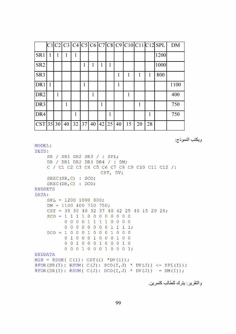
C1 C2 C3 C4 C5 C6 C7 C8 C9 C10 C11 C12 SPL DM
SR1 1 1 1 1 1200
SR2 1 1 1 1 1000
SR3 1 1 1 1 800
DR1 1 1 1 1100
DR2 1 1 1 400
DR3 1 1 1 750
DR4 1 1 1 750
CST 35 30 40 32 37 40 42 25 40 15 20 28
ويكتب النموذج:
والتقرير: يترك للطالب كتمرين.
100
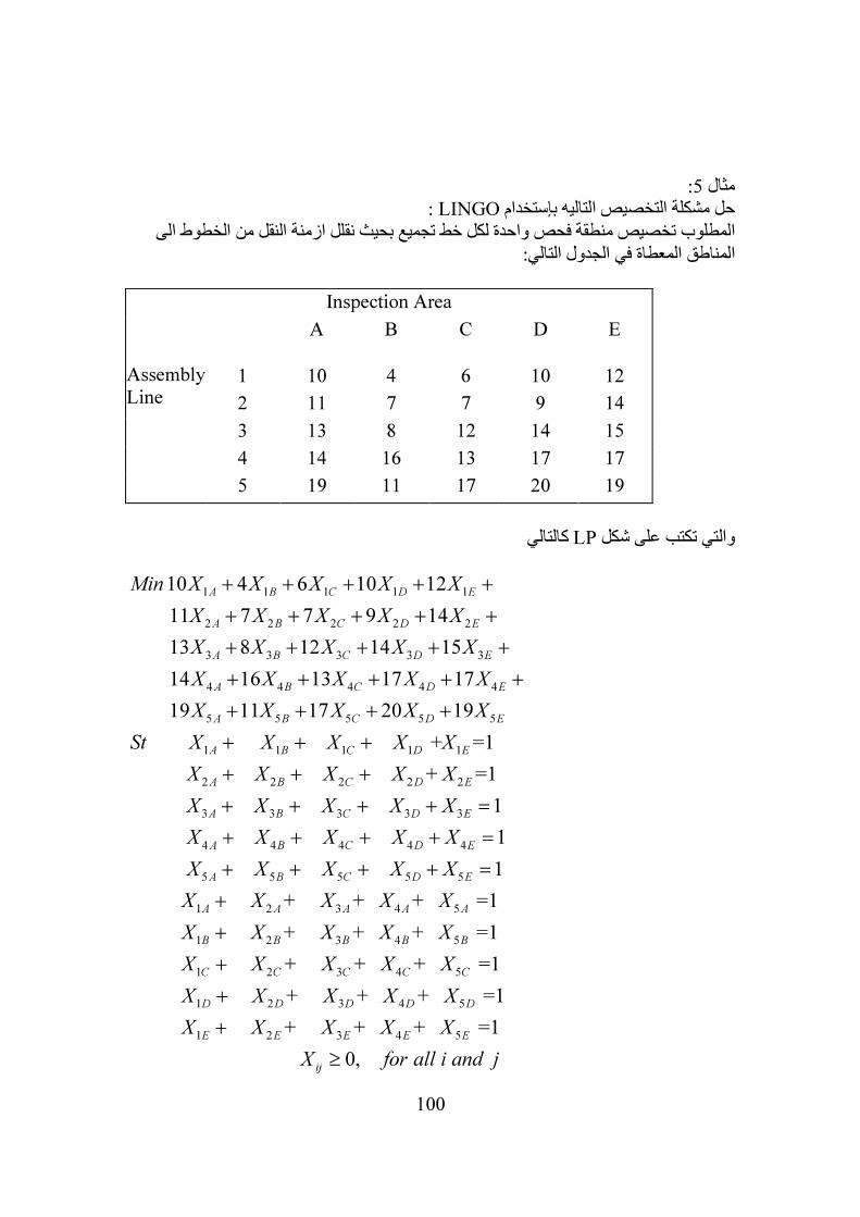
:5مثال
: LINGOتخدام حل مشكلة التخصيص التاليه بإسالمطلوب تخصيص منطقة فحص واحدة لكل خط تجميع بحيث نقلل ازمنة النقل من الخطوط الى
المناطق المعطاة في الجدول التالي:
Inspection Area AssemblyLine
A B C D E
1 10 4 6 10 12 2 11 7 7 9 14 3 13 8 12 14 15 4 14 16 13 17 17 5 19 11 17 20 19
كالتالي LPوالتي تكتب على شكل
1 1 1 1 1
2 2 2 2 2
3 3 3 3 3
4 4 4 4 4
5 5 5 5 5
1 1 1 1 1
2 2 2 2
10 4 6 10 12
11 7 7 9 14
13 8 12 14 15
14 16 13 17 17
19 11 17 20 19
+ =1
+
A B C D E
A B C D E
A B C D E
A B C D E
A B C D E
A B C D E
A B C D
Min X X X X X
X X X X X
X X X X X
X X X X X
X X X X X
St X X X X X
X X X X
+ + + + +
+ + + + +
+ + + + +
+ + + + +
+ + + +
+ + +
+ + +2
3 3 3 3 3
4 4 4 4 4
5 5 5 5 5
1 2 3 4 5
1 2 3 4 5
=1
1
1
1
+ + + =1
+ + + =1
E
A B C D E
A B C D E
A B C D E
A A A A A
B B B B B
X
X X X X X
X X X X X
X X X X X
X X X X X
X X X X X
+ + + + =
+ + + + =
+ + + + =
+
+
1 2 3 4 5
1 2 3 4 5
1 2 3 4 5
+ + + =1
+ + + =1
+ + + =1
0,
C C C C C
D D D D D
E E E E E
ij
X X X X X
X X X X X
X X X X X
X for all i and j
+
+
+
≥
101
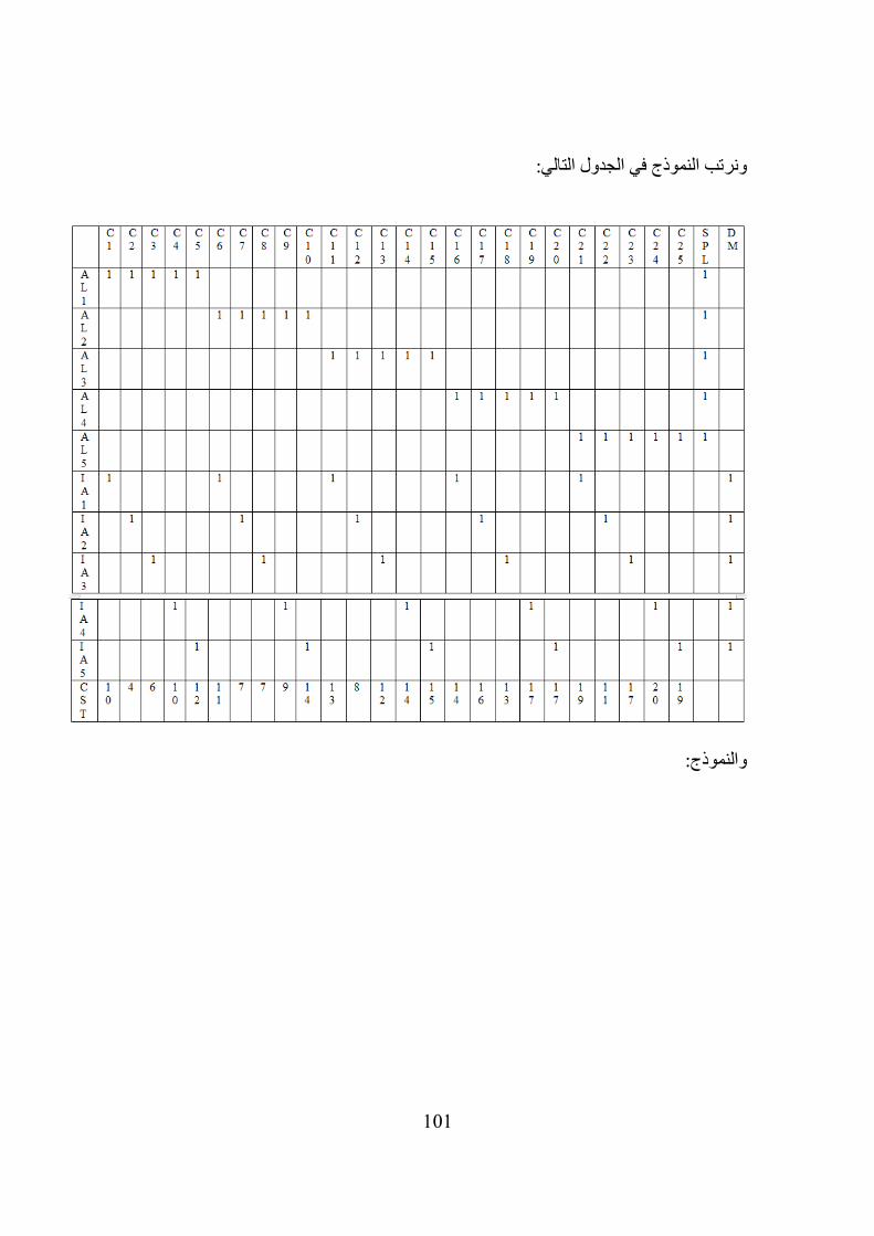
ونرتب النموذج في الجدول التالي:
والنموذج:
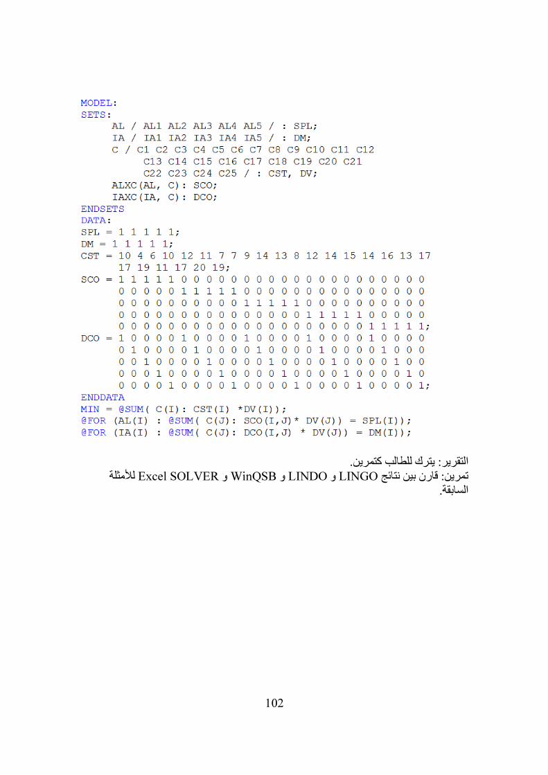
102
التقرير: يترك للطالب كتمرين.لألمثلة Excel SOLVERو WinQSBو LINDOو LINGOقارن بين نتائج :تمرين
السابقة.
103
:6مثال : الشبكة التالية تمثل خطوط سير ممكنة للسفر من Shortest Path Problemمشكلة أقصر طريق
( عقدة النهاية) والمراد تعيين أقصر مسافة لخط السير. 12(عقدة البداية) إلى العقدة 1العقدة
إليجاد مسافة أقصر طريق عبر الشبكة سوف نستخدم التكرار التالي للبرمجة الديناميكية: إلى iهي المسافة من العقدة D(i,j) إلى العقدة النهائية و iأقل مسافة إنتقال من العقدة F(i) حيث
األقل بين كل العقد التي يمكن إلى العقدة النهائية هي تلك i. أي أن أقل مسافة من العقدة jالعقدة
12
3 4
5
6
7
8
9
10
11
12
599
180
497
432
345420
440
691
893
280
500
290
577
116
403
314
432 6
21
554
( ) ( ) ( ),
jF i MIN D i j F j= +
104
إلى العقدة المجاورة مضاف إليها أقل iلمجموع المسافات من iالوصول إليها عبر قوس واحد من مسافة من العقدة المجاورة إلى العقدة النهائية.
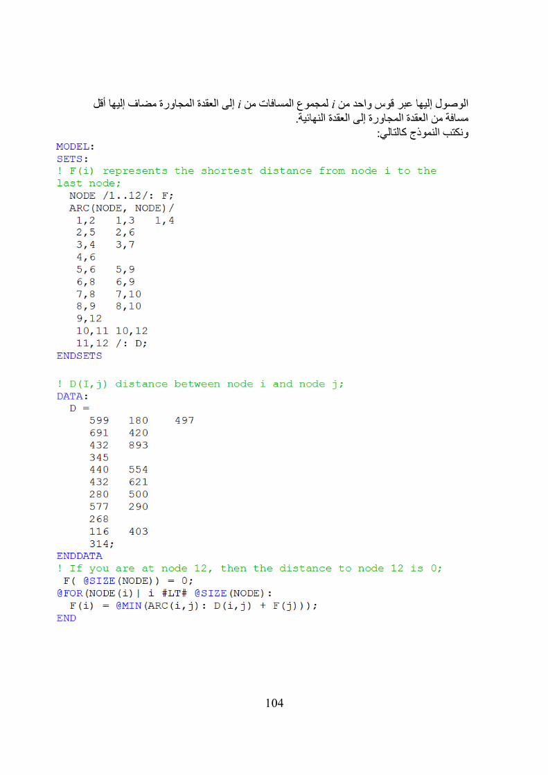
ونكتب النموذج كالتالي:
105
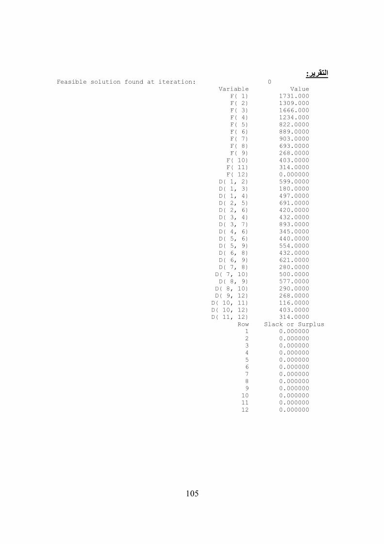
:التقريرFeasible solution found at iteration: 0 Variable Value F( 1) 1731.000 F( 2) 1309.000 F( 3) 1666.000 F( 4) 1234.000 F( 5) 822.0000 F( 6) 889.0000 F( 7) 903.0000 F( 8) 693.0000 F( 9) 268.0000 F( 10) 403.0000 F( 11) 314.0000 F( 12) 0.000000 D( 1, 2) 599.0000 D( 1, 3) 180.0000 D( 1, 4) 497.0000 D( 2, 5) 691.0000 D( 2, 6) 420.0000 D( 3, 4) 432.0000 D( 3, 7) 893.0000 D( 4, 6) 345.0000 D( 5, 6) 440.0000 D( 5, 9) 554.0000 D( 6, 8) 432.0000 D( 6, 9) 621.0000 D( 7, 8) 280.0000 D( 7, 10) 500.0000 D( 8, 9) 577.0000 D( 8, 10) 290.0000 D( 9, 12) 268.0000 D( 10, 11) 116.0000 D( 10, 12) 403.0000 D( 11, 12) 314.0000 Row Slack or Surplus 1 0.000000 2 0.000000 3 0.000000 4 0.000000 5 0.000000 6 0.000000 7 0.000000 8 0.000000 9 0.000000 10 0.000000 11 0.000000 12 0.000000

106
:1 تمرين للشبكة التالية: 11إلى القرار 1أوجد أقصر طريق من المصدر
:2تمرين رن النتائج.وقا Excel Solverحل التمرين السابق بواسطة
1
2
3
4
5
6
7
8
9
10
116
4
3
5
3
4
6
2
2
5
2
1
4
2
5
3
5
8
4
7
4
2
107
:7مثال :Maximal Flow Problemمشكلة التدفق األعظم
الشبكة التالية تمثل تمديدات ألنابيب ماء في شبكة تمد خزان بالمياه
1
23
45
6
7
1010
1 1
4
4
12
2
2
68
7
3
3
2
8
12
Source
Tank
جالون/دقيقة) 1000الجدول التالي يعطي سعة األنابيب (
TO 7 6 5 4 3 2 1 F
R O M
10 10 1 6 8 1 2 4 12 1 3 7 3 4 8 2 5 2 2 3 4 6
7
المطلوب تحديد مسار أقصى تدفق للخزان.
108
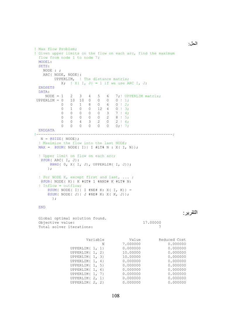
الحل:! Max flow Problem; ! Given upper limits on the flow on each arc, find the maximum flow from node 1 to node 7; MODEL: SETS: NODE : ; ARC( NODE, NODE): UPPERLIM, ! The distance matrix; X; ! X( I, J) = 1 if we use ARC I, J; ENDSETS DATA: NODE = 1 2 3 4 5 6 7;! UPPERLIM matrix; UPPERLIM = 0 10 10 0 0 0 0 ! 1; 0 0 1 8 0 6 0 ! 2; 0 1 0 0 12 4 0 ! 3; 0 0 0 0 0 3 7 ! 4; 0 0 0 0 0 2 8 ! 5; 0 0 4 3 2 0 2 ! 6; 0 0 0 0 0 0 0;! 7; ENDDATA !------------------------------------------------------------; N = @SIZE( NODE); ! Maximize the flow into the last NODE; MAX = @SUM( NODE( I)| I #LT# N : X( I, N)); ! Upper limit on flow on each arc; @FOR( ARC( I, J): @BND( 0, X( I, J), UPPERLIM( I, J)); ); ! For NODE K, except first and last, ... ; @FOR( NODE( K)| K #GT# 1 #AND# K #LT# N: ! Inflow = outflow; @SUM( NODE( I)| I #NE# K: X( I, K)) = @SUM( NODE( J)| J #NE# K: X( K, J)); ); END
التقرير: Global optimal solution found. Objective value: 17.00000 Total solver iterations: 7 Variable Value Reduced Cost N 7.000000 0.000000 UPPERLIM( 1, 1) 0.000000 0.000000 UPPERLIM( 1, 2) 10.00000 0.000000 UPPERLIM( 1, 3) 10.00000 0.000000 UPPERLIM( 1, 4) 0.000000 0.000000 UPPERLIM( 1, 5) 0.000000 0.000000 UPPERLIM( 1, 6) 0.000000 0.000000 UPPERLIM( 1, 7) 0.000000 0.000000 UPPERLIM( 2, 1) 0.000000 0.000000 UPPERLIM( 2, 2) 0.000000 0.000000
109
UPPERLIM( 2, 3) 1.000000 0.000000 UPPERLIM( 2, 4) 8.000000 0.000000 UPPERLIM( 2, 5) 0.000000 0.000000 UPPERLIM( 2, 6) 6.000000 0.000000 UPPERLIM( 2, 7) 0.000000 0.000000 UPPERLIM( 3, 1) 0.000000 0.000000 UPPERLIM( 3, 2) 1.000000 0.000000 UPPERLIM( 3, 3) 0.000000 0.000000 UPPERLIM( 3, 4) 0.000000 0.000000 UPPERLIM( 3, 5) 12.00000 0.000000 UPPERLIM( 3, 6) 4.000000 0.000000 UPPERLIM( 3, 7) 0.000000 0.000000 UPPERLIM( 4, 1) 0.000000 0.000000 UPPERLIM( 4, 2) 0.000000 0.000000 UPPERLIM( 4, 3) 0.000000 0.000000 UPPERLIM( 4, 4) 0.000000 0.000000 UPPERLIM( 4, 5) 0.000000 0.000000 UPPERLIM( 4, 6) 3.000000 0.000000 UPPERLIM( 4, 7) 7.000000 0.000000 UPPERLIM( 5, 1) 0.000000 0.000000 UPPERLIM( 5, 2) 0.000000 0.000000 UPPERLIM( 5, 3) 0.000000 0.000000 UPPERLIM( 5, 4) 0.000000 0.000000 UPPERLIM( 5, 5) 0.000000 0.000000 UPPERLIM( 5, 6) 2.000000 0.000000 UPPERLIM( 5, 7) 8.000000 0.000000 UPPERLIM( 6, 1) 0.000000 0.000000 UPPERLIM( 6, 2) 0.000000 0.000000 UPPERLIM( 6, 3) 4.000000 0.000000 UPPERLIM( 6, 4) 3.000000 0.000000 UPPERLIM( 6, 5) 2.000000 0.000000 UPPERLIM( 6, 6) 0.000000 0.000000 UPPERLIM( 6, 7) 2.000000 0.000000 UPPERLIM( 7, 1) 0.000000 0.000000 UPPERLIM( 7, 2) 0.000000 0.000000 UPPERLIM( 7, 3) 0.000000 0.000000 UPPERLIM( 7, 4) 0.000000 0.000000 UPPERLIM( 7, 5) 0.000000 0.000000 UPPERLIM( 7, 6) 0.000000 0.000000 UPPERLIM( 7, 7) 0.000000 0.000000 X( 1, 1) 0.000000 0.000000 X( 1, 2) 7.000000 0.000000 X( 1, 3) 10.00000 0.000000 X( 1, 4) 0.000000 0.000000 X( 1, 5) 0.000000 0.000000 X( 1, 6) 0.000000 0.000000 X( 1, 7) 0.000000 -1.000000 X( 2, 1) 0.000000 0.000000 X( 2, 2) 0.000000 0.000000 X( 2, 3) 0.000000 0.000000 X( 2, 4) 4.000000 0.000000 X( 2, 5) 0.000000 0.000000 X( 2, 6) 4.000000 0.000000 X( 2, 7) 0.000000 -1.000000 X( 3, 1) 0.000000 0.000000 X( 3, 2) 1.000000 0.000000 X( 3, 3) 0.000000 0.000000
110
X( 3, 4) 0.000000 0.000000 X( 3, 5) 6.000000 0.000000 X( 3, 6) 3.000000 0.000000 X( 3, 7) 0.000000 -1.000000 X( 4, 1) 0.000000 0.000000 X( 4, 2) 0.000000 0.000000 X( 4, 3) 0.000000 0.000000 X( 4, 4) 0.000000 0.000000 X( 4, 5) 0.000000 0.000000 X( 4, 6) 0.000000 0.000000 X( 4, 7) 7.000000 -1.000000 X( 5, 1) 0.000000 0.000000 X( 5, 2) 0.000000 0.000000 X( 5, 3) 0.000000 0.000000 X( 5, 4) 0.000000 0.000000 X( 5, 5) 0.000000 0.000000 X( 5, 6) 0.000000 0.000000 X( 5, 7) 8.000000 -1.000000 X( 6, 1) 0.000000 0.000000 X( 6, 2) 0.000000 0.000000 X( 6, 3) 0.000000 0.000000 X( 6, 4) 3.000000 0.000000 X( 6, 5) 2.000000 0.000000 X( 6, 6) 0.000000 0.000000 X( 6, 7) 2.000000 -1.000000 X( 7, 1) 0.000000 0.000000 X( 7, 2) 0.000000 0.000000 X( 7, 3) 0.000000 0.000000 X( 7, 4) 0.000000 0.000000 X( 7, 5) 0.000000 0.000000 X( 7, 6) 0.000000 0.000000 X( 7, 7) 0.000000 0.000000 Row Slack or Surplus Dual Price 1 0.000000 0.000000 2 17.00000 1.000000 3 0.000000 0.000000 4 0.000000 0.000000 5 0.000000 0.000000 6 0.000000 0.000000 7 0.000000 0.000000
111
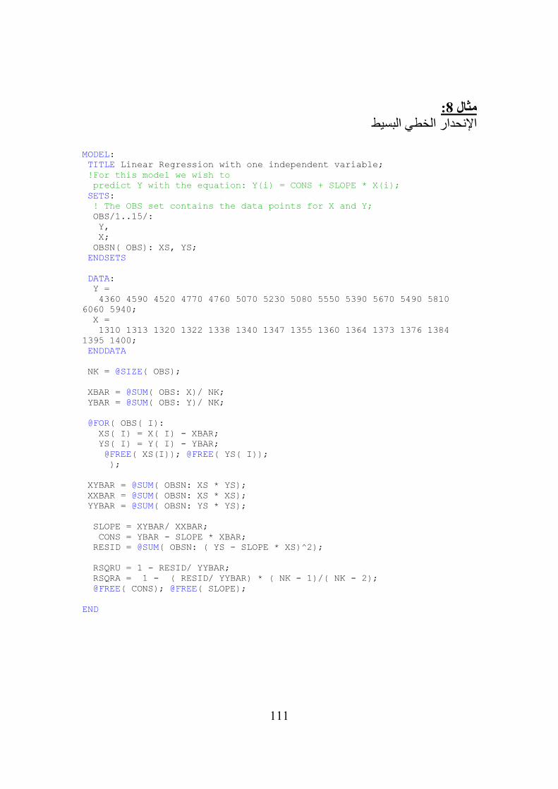
:8مثال
اإلنحدار الخطي البسيط
MODEL: TITLE Linear Regression with one independent variable; !For this model we wish to predict Y with the equation: Y(i) = CONS + SLOPE * X(i); SETS: ! The OBS set contains the data points for X and Y; OBS/1..15/: Y, X; OBSN( OBS): XS, YS; ENDSETS DATA: Y = 4360 4590 4520 4770 4760 5070 5230 5080 5550 5390 5670 5490 5810 6060 5940; X = 1310 1313 1320 1322 1338 1340 1347 1355 1360 1364 1373 1376 1384 1395 1400; ENDDATA NK = @SIZE( OBS); XBAR = @SUM( OBS: X)/ NK; YBAR = @SUM( OBS: Y)/ NK; @FOR( OBS( I): XS( I) = X( I) - XBAR; YS( I) = Y( I) - YBAR; @FREE( XS(I)); @FREE( YS( I)); ); XYBAR = @SUM( OBSN: XS * YS); XXBAR = @SUM( OBSN: XS * XS); YYBAR = @SUM( OBSN: YS * YS); SLOPE = XYBAR/ XXBAR; CONS = YBAR - SLOPE * XBAR; RESID = @SUM( OBSN: ( YS - SLOPE * XS)^2); RSQRU = 1 - RESID/ YYBAR; RSQRA = 1 - ( RESID/ YYBAR) * ( NK - 1)/( NK - 2); @FREE( CONS); @FREE( SLOPE); END
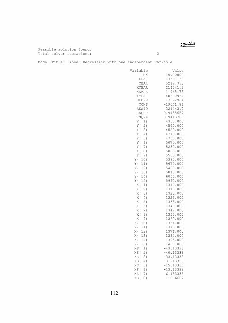
112
النتائج: Feasible solution found. Total solver iterations: 0 Model Title: Linear Regression with one independent variable Variable Value NK 15.00000 XBAR 1353.133 YBAR 5219.333 XYBAR 214541.3 XXBAR 11965.73 YYBAR 4068093. SLOPE 17.92964 CONS -19041.86 RESID 221443.7 RSQRU 0.9455657 RSQRA 0.9413785 Y( 1) 4360.000 Y( 2) 4590.000 Y( 3) 4520.000 Y( 4) 4770.000 Y( 5) 4760.000 Y( 6) 5070.000 Y( 7) 5230.000 Y( 8) 5080.000 Y( 9) 5550.000 Y( 10) 5390.000 Y( 11) 5670.000 Y( 12) 5490.000 Y( 13) 5810.000 Y( 14) 6060.000 Y( 15) 5940.000 X( 1) 1310.000 X( 2) 1313.000 X( 3) 1320.000 X( 4) 1322.000 X( 5) 1338.000 X( 6) 1340.000 X( 7) 1347.000 X( 8) 1355.000 X( 9) 1360.000 X( 10) 1364.000 X( 11) 1373.000 X( 12) 1376.000 X( 13) 1384.000 X( 14) 1395.000 X( 15) 1400.000 XS( 1) -43.13333 XS( 2) -40.13333 XS( 3) -33.13333 XS( 4) -31.13333 XS( 5) -15.13333 XS( 6) -13.13333 XS( 7) -6.133333 XS( 8) 1.866667
113
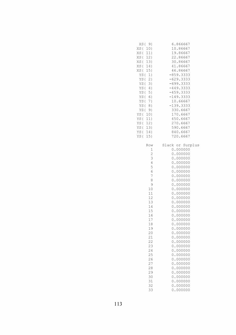
XS( 9) 6.866667 XS( 10) 10.86667 XS( 11) 19.86667 XS( 12) 22.86667 XS( 13) 30.86667 XS( 14) 41.86667 XS( 15) 46.86667 YS( 1) -859.3333 YS( 2) -629.3333 YS( 3) -699.3333 YS( 4) -449.3333 YS( 5) -459.3333 YS( 6) -149.3333 YS( 7) 10.66667 YS( 8) -139.3333 YS( 9) 330.6667 YS( 10) 170.6667 YS( 11) 450.6667 YS( 12) 270.6667 YS( 13) 590.6667 YS( 14) 840.6667 YS( 15) 720.6667 Row Slack or Surplus 1 0.000000 2 0.000000 3 0.000000 4 0.000000 5 0.000000 6 0.000000 7 0.000000 8 0.000000 9 0.000000 10 0.000000 11 0.000000 12 0.000000 13 0.000000 14 0.000000 15 0.000000 16 0.000000 17 0.000000 18 0.000000 19 0.000000 20 0.000000 21 0.000000 22 0.000000 23 0.000000 24 0.000000 25 0.000000 26 0.000000 27 0.000000 28 0.000000 29 0.000000 30 0.000000 31 0.000000 32 0.000000 33 0.000000

114
34 0.000000 35 0.000000 36 0.000000 37 0.000000 38 0.000000 39 0.000000 40 0.000000 41 0.000000
115
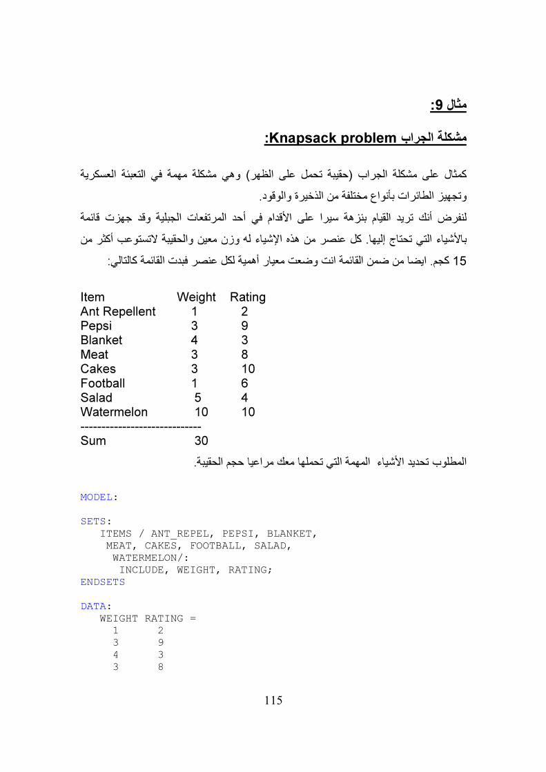
:9مثال
:Knapsack problemمشكلة الجراب
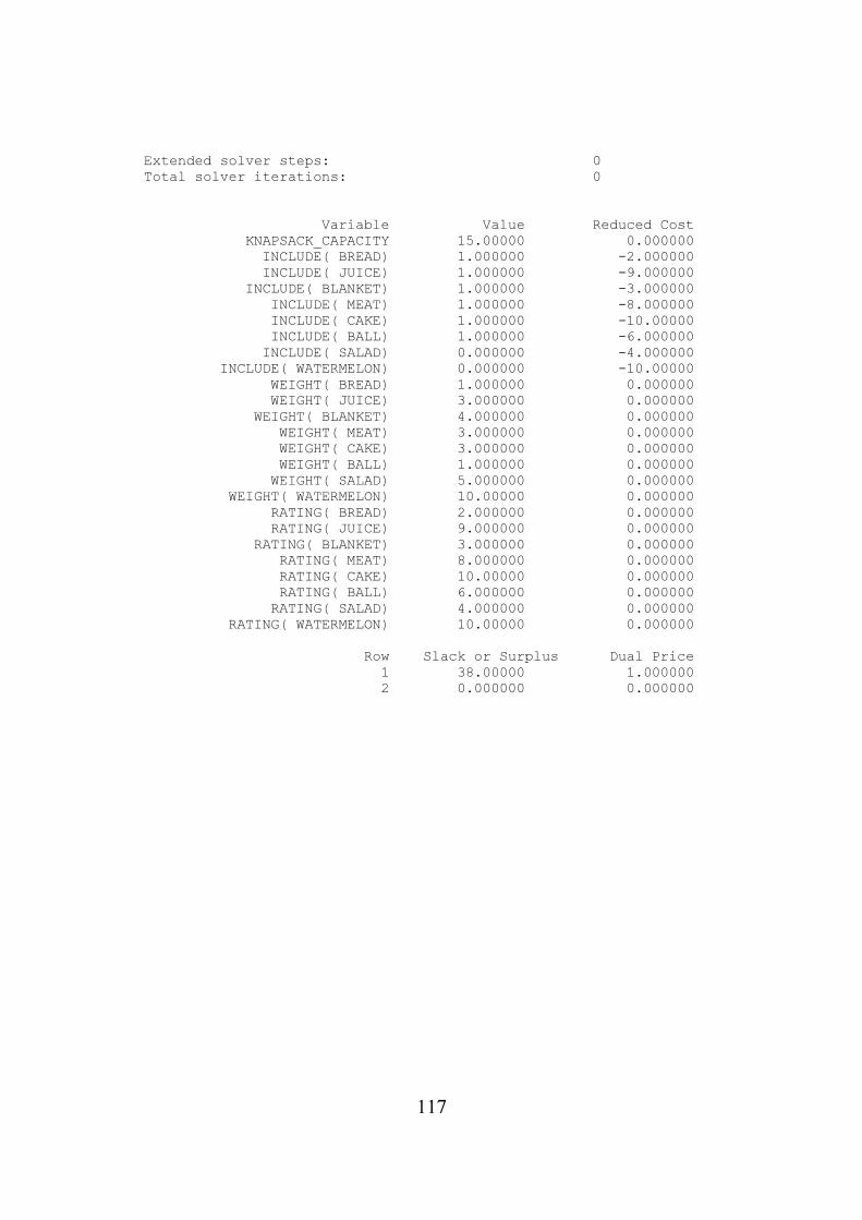
كمثال على مشكلة الجراب (حقيبة تحمل على الظهر) وهي مشكلة مهمة في التعبئة العسكرية
وتجهيز الطائرات بأنواع مختلفة من الذخيرة والوقود.
لنفرض أنك تريد القيام بنزهة سيرا على األقدام في أحد المرتفعات الجبلية وقد جهزت قائمة
باألشياء التي تحتاج إليها. كل عنصر من هذه اإلشياء له وزن معين والحقيبة التستوعب أكثر من
كجم. ايضا من ضمن القائمة انت وضعت معيار أهمية لكل عنصر فبدت القائمة كالتالي: 15
Item Weight Rating Ant Repellent 1 2 Pepsi 3 9 Blanket 4 3 Meat 3 8 Cakes 3 10 Football 1 6 Salad 5 4 Watermelon 10 10 ----------------------------- Sum 30
المطلوب تحديد األشياء المهمة التي تحملها معك مراعيا حجم الحقيبة.
MODEL: SETS: ITEMS / ANT_REPEL, PEPSI, BLANKET, MEAT, CAKES, FOOTBALL, SALAD, WATERMELON/: INCLUDE, WEIGHT, RATING; ENDSETS DATA: WEIGHT RATING = 1 2 3 9 4 3 3 8
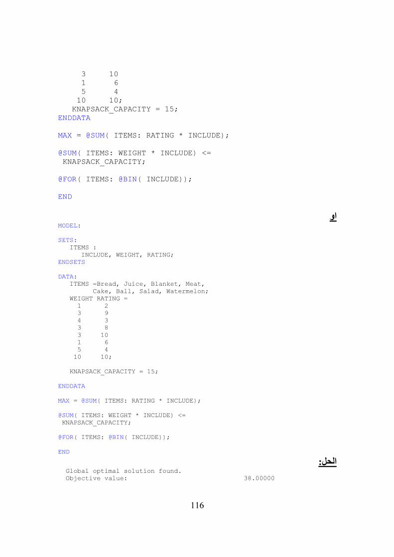
116
3 10 1 6 5 4 10 10; KNAPSACK_CAPACITY = 15; ENDDATA MAX = @SUM( ITEMS: RATING * INCLUDE); @SUM( ITEMS: WEIGHT * INCLUDE) <= KNAPSACK_CAPACITY; @FOR( ITEMS: @BIN( INCLUDE)); END
اوMODEL: SETS: ITEMS : INCLUDE, WEIGHT, RATING; ENDSETS DATA: ITEMS =Bread, Juice, Blanket, Meat, Cake, Ball, Salad, Watermelon; WEIGHT RATING = 1 2 3 9 4 3 3 8 3 10 1 6 5 4 10 10; KNAPSACK_CAPACITY = 15; ENDDATA MAX = @SUM( ITEMS: RATING * INCLUDE); @SUM( ITEMS: WEIGHT * INCLUDE) <= KNAPSACK_CAPACITY; @FOR( ITEMS: @BIN( INCLUDE)); END
الحل: Global optimal solution found. Objective value: 38.00000
117
Extended solver steps: 0 Total solver iterations: 0 Variable Value Reduced Cost KNAPSACK_CAPACITY 15.00000 0.000000 INCLUDE( BREAD) 1.000000 -2.000000 INCLUDE( JUICE) 1.000000 -9.000000 INCLUDE( BLANKET) 1.000000 -3.000000 INCLUDE( MEAT) 1.000000 -8.000000 INCLUDE( CAKE) 1.000000 -10.00000 INCLUDE( BALL) 1.000000 -6.000000 INCLUDE( SALAD) 0.000000 -4.000000 INCLUDE( WATERMELON) 0.000000 -10.00000 WEIGHT( BREAD) 1.000000 0.000000 WEIGHT( JUICE) 3.000000 0.000000 WEIGHT( BLANKET) 4.000000 0.000000 WEIGHT( MEAT) 3.000000 0.000000 WEIGHT( CAKE) 3.000000 0.000000 WEIGHT( BALL) 1.000000 0.000000 WEIGHT( SALAD) 5.000000 0.000000 WEIGHT( WATERMELON) 10.00000 0.000000 RATING( BREAD) 2.000000 0.000000 RATING( JUICE) 9.000000 0.000000 RATING( BLANKET) 3.000000 0.000000 RATING( MEAT) 8.000000 0.000000 RATING( CAKE) 10.00000 0.000000 RATING( BALL) 6.000000 0.000000 RATING( SALAD) 4.000000 0.000000 RATING( WATERMELON) 10.00000 0.000000 Row Slack or Surplus Dual Price 1 38.00000 1.000000 2 0.000000 0.000000
118
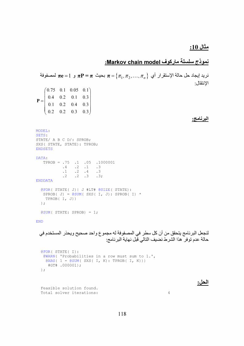
:10مثال
:Markov chain model نموذج سلسلة ماركوف
}نريد إيجاد حل حالة اإلستقرار أي }1 2 n, , ,π π π=π πPبحيث … = π 1و=πe مصفوفة ل
اإلنتقال: 0 75 0 1 0 05 0 1
0 4 0 2 0 1 0 3
0 1 0 2 0 4 0 3
0 2 0 2 0 3 0 3
. . . .
. . . .
. . . .
. . . .
=
P
البرنامج:
MODEL: SETS: STATE/ A B C D/: SPROB; SXS( STATE, STATE): TPROB; ENDSETS DATA: TPROB = .75 .1 .05 .1000001 .4 .2 .1 .3 .1 .2 .4 .3 .2 .2 .3 .3; ENDDATA @FOR( STATE( J)| J #LT# @SIZE( STATE): SPROB( J) = @SUM( SXS( I, J): SPROB( I) * TPROB( I, J)) ); @SUM( STATE: SPROB) = 1; END
لنجعل البرنامج يتحقق من أن كل سطر في المصفوفة له مجموع واحد صحيح ويحذر المستخدم في
ط نضيف التالي قبل نهاية البرنامج:حالة عدم توفر هذا الشر @FOR( STATE( I): @WARN( 'Probabilities in a row must sum to 1.', @ABS( 1 - @SUM( SXS( I, K): TPROB( I, K))) #GT# .000001); );
الحل:
Feasible solution found. Total solver iterations: 4
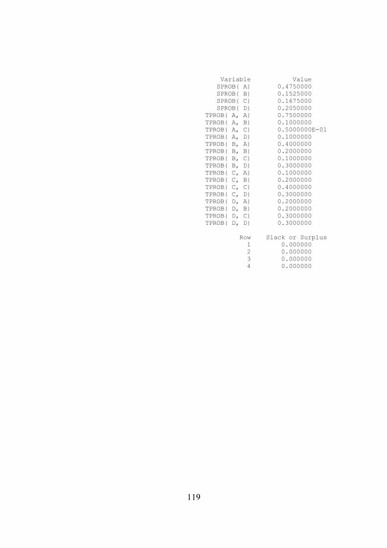
119
Variable Value SPROB( A) 0.4750000 SPROB( B) 0.1525000 SPROB( C) 0.1675000 SPROB( D) 0.2050000 TPROB( A, A) 0.7500000 TPROB( A, B) 0.1000000 TPROB( A, C) 0.5000000E-01 TPROB( A, D) 0.1000000 TPROB( B, A) 0.4000000 TPROB( B, B) 0.2000000 TPROB( B, C) 0.1000000 TPROB( B, D) 0.3000000 TPROB( C, A) 0.1000000 TPROB( C, B) 0.2000000 TPROB( C, C) 0.4000000 TPROB( C, D) 0.3000000 TPROB( D, A) 0.2000000 TPROB( D, B) 0.2000000 TPROB( D, C) 0.3000000 TPROB( D, D) 0.3000000 Row Slack or Surplus 1 0.000000 2 0.000000 3 0.000000 4 0.000000
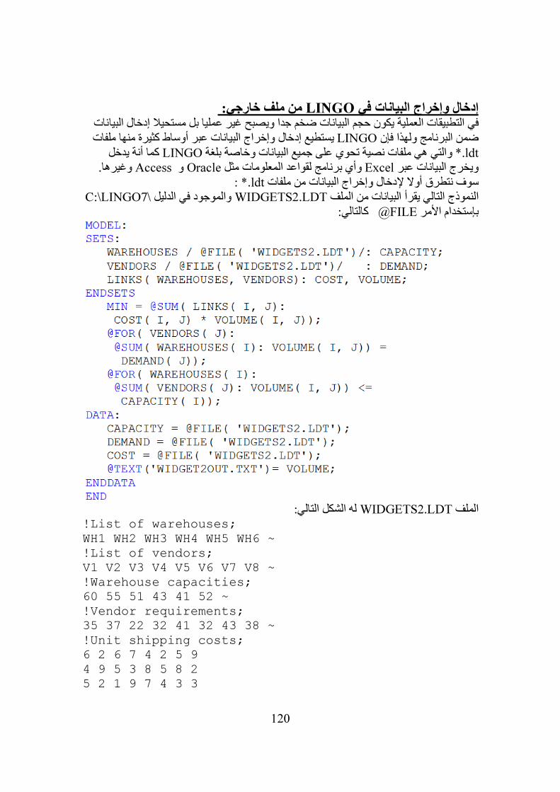
120
من ملف خارجي: LINGOإدخال وإخراج البيانات في
في التطبيقات العملية يكون حجم البيانات ضخم جدا ويصبح غير عمليا بل مستحيال إدخال البيانات يستطيع إدخال وإخراج البيانات عبر أوساط كثيرة منها ملفات LINGOضمن البرنامج ولهذا فإن
*.ldt ميع البيانات وخاصة بلغة والتي هي ملفات نصية تحوي على جLINGO كما أنة يدخل وغيرها. Accessو Oracleوأي برنامج لقواعد المعلومات مثل Excelويخرج البيانات عبر
: ldt.*سوف نتطرق أوال إلدخال وإخراج البيانات من ملفات \C:\LINGO7والموجود في الدليل WIDGETS2.LDTالنموذج التالي يقرأ البيانات من الملف
كالتالي: FILE@بإستخدام األمر
له الشكل التالي: WIDGETS2.LDTالملف
!List of warehouses; WH1 WH2 WH3 WH4 WH5 WH6 ~ !List of vendors; V1 V2 V3 V4 V5 V6 V7 V8 ~ !Warehouse capacities; 60 55 51 43 41 52 ~ !Vendor requirements; 35 37 22 32 41 32 43 38 ~ !Unit shipping costs; 6 2 6 7 4 2 5 9 4 9 5 3 8 5 8 2 5 2 1 9 7 4 3 3
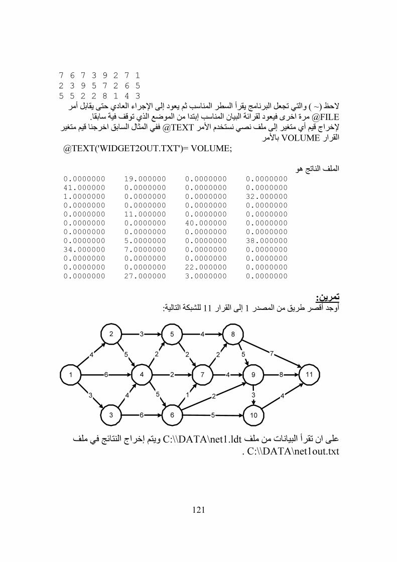
121
7 6 7 3 9 2 7 1 2 3 9 5 7 2 6 5 5 5 2 2 8 1 4 3
) والتي تجعل البرنامج يقرأ السطر المناسب ثم يعود إلى اإلجراء العادي حتى يقابل أمر ~الحظ (@FILE عود لقرائة البيان المناسب إبتدا من الموضع الذي توقف فية سابقا.مرة اخرى في
ففي المثال السابق اخرجنا قيم متغير TEXT@إلخراج قيم أي متغير إلى ملف نصي نستخدم األمر باألمر VOLUMEالقرار
@TEXT('WIDGET2OUT.TXT')= VOLUME;
الملف الناتج هو 0.0000000 19.000000 0.0000000 0.0000000 41.000000 0.0000000 0.0000000 0.0000000 1.0000000 0.0000000 0.0000000 32.000000 0.0000000 0.0000000 0.0000000 0.0000000 0.0000000 11.000000 0.0000000 0.0000000 0.0000000 0.0000000 40.000000 0.0000000 0.0000000 0.0000000 0.0000000 0.0000000 0.0000000 5.0000000 0.0000000 38.000000 34.000000 7.0000000 0.0000000 0.0000000 0.0000000 0.0000000 0.0000000 0.0000000 0.0000000 0.0000000 22.000000 0.0000000 0.0000000 27.000000 3.0000000 0.0000000
تمرين:
للشبكة التالية: 11إلى القرار 1أوجد أقصر طريق من المصدر
ويتم إخراج النتائج في ملف C:\\DATA\net1.ldtعلى ان تقرأ البيانات من ملف net1out.txt\DATA\\C: .
1
2
3
4
5
6
7
8
9
10
116
4
3
5
3
4
6
2
2
5
2
1
4
2
5
3
5
8
4
7
4
2
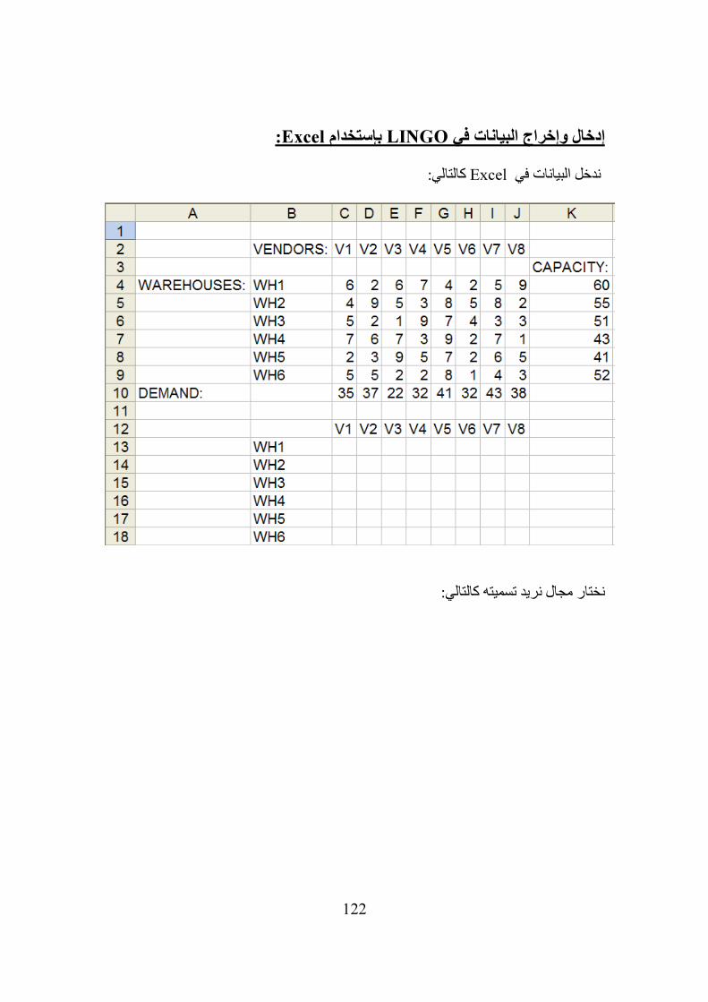
122
:Excelبإستخدام OLINGإدخال وإخراج البيانات في كالتالي: Excelندخل البيانات في
نختار مجال نريد تسميته كالتالي:
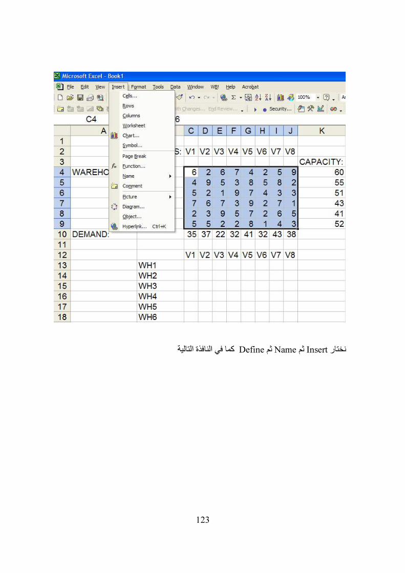
123
كما في النافذة التالية Defineثم Nameثم Insertنختار
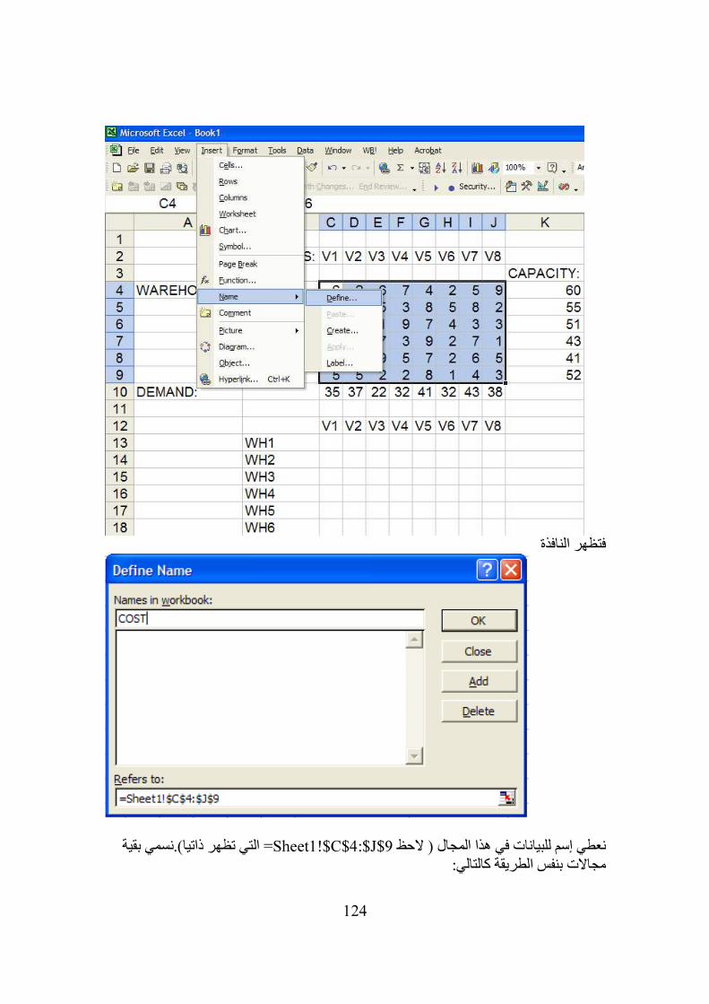
124
فتظهر النافذة
التي تظهر ذاتيا).نسمي بقية Sheet1!$C$4:$J$9=نعطي إسم للبيانات في هذا المجال ( الحظ مجاالت بنفس الطريقة كالتالي:
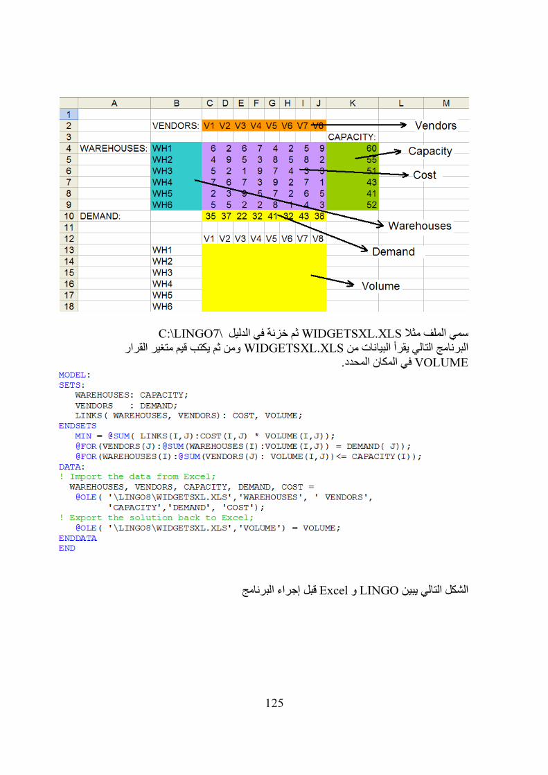
125
\C:\LINGO7ثم خزنة في الدليل WIDGETSXL.XLSسمي الملف مثال ومن ثم يكتب قيم متغير القرار WIDGETSXL.XLSت من البرنامج التالي يقرأ البيانا
VOLUME .في المكان المحدد
قبل إجراء البرنامج Excelو LINGOالشكل التالي يبين
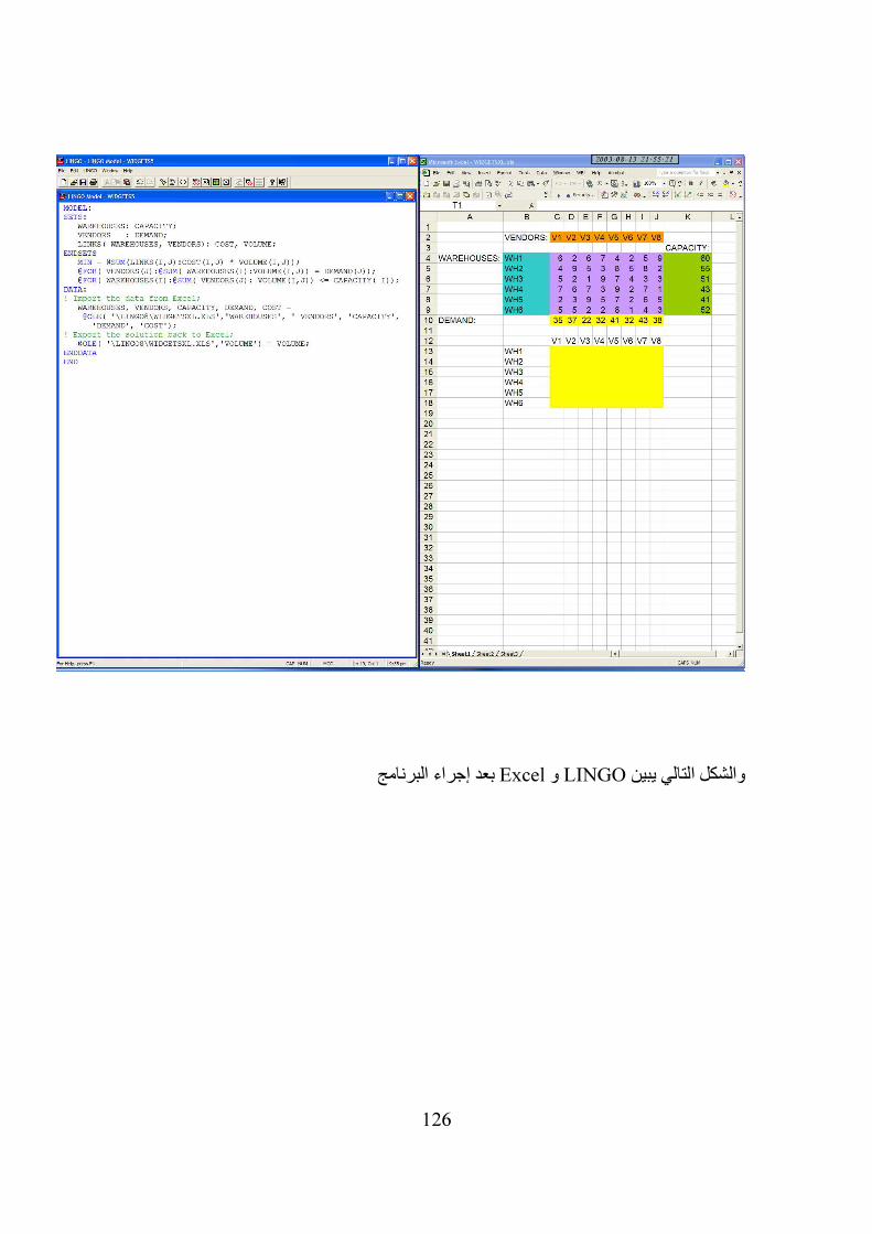
126
بعد إجراء البرنامج Excelو LINGOالشكل التالي يبين و
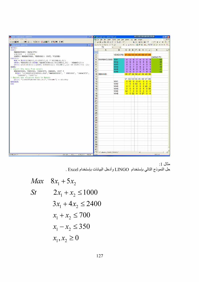
127
:1مثال . Excelالبيانات بإستخدام وأدخل LINGOحل النموذج التالي بإستخدام
1 2
1 2
1 2
1 2
1 2
1 2
8 5
2 1000
3 4 2400
700
350
, 0
Max x x
St x x
x x
x x
x x
x x
+
+ ≤
+ ≤
+ ≤
− ≤
≥
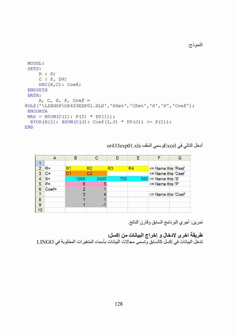
128
النموذج:
or433exp01.xlsوسمي الملف Excelأدخل التالي في
ن الناتج.تمرين: أجري البرنامج السابق وقار
طريقة اخرى إلدخال و إخراج البيانات من إكسل:
LINGOتدخل البيانات في إكسل كالسابق وتسمى مجاالت البيانات بأسماء المتغيرات المطلوبة في
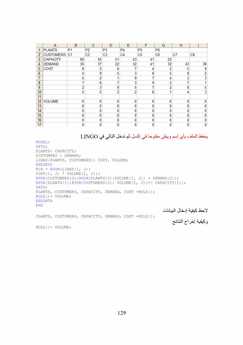
129
LINGOثم ندخل التالي في يحفظ الملف بأي إسم ويبقى مفتوحا في إكسل MODEL: SETS: PLANTS: CAPACITY; CUSTOMERS : DEMAND; LINKS(PLANTS, CUSTOMERS): COST, VOLUME; ENDSETS MIN = @SUM(LINKS(I, J): COST(I, J) * VOLUME(I, J)); @FOR(CUSTOMERS(J):@SUM(PLANTS(I):VOLUME(I, J)) = DEMAND(J)); @FOR(PLANTS(I):@SUM(CUSTOMERS(J): VOLUME(I, J))<= CAPACITY(I)); DATA: PLANTS, CUSTOMERS, CAPACITY, DEMAND, COST =@OLE(); @OLE()= VOLUME; ENDDATA END
الحظ كيفية إدخال البيانات PLANTS, CUSTOMERS, CAPACITY, DEMAND, COST =@OLE();
وكيفية إخراج النتائج@OLE()= VOLUME;
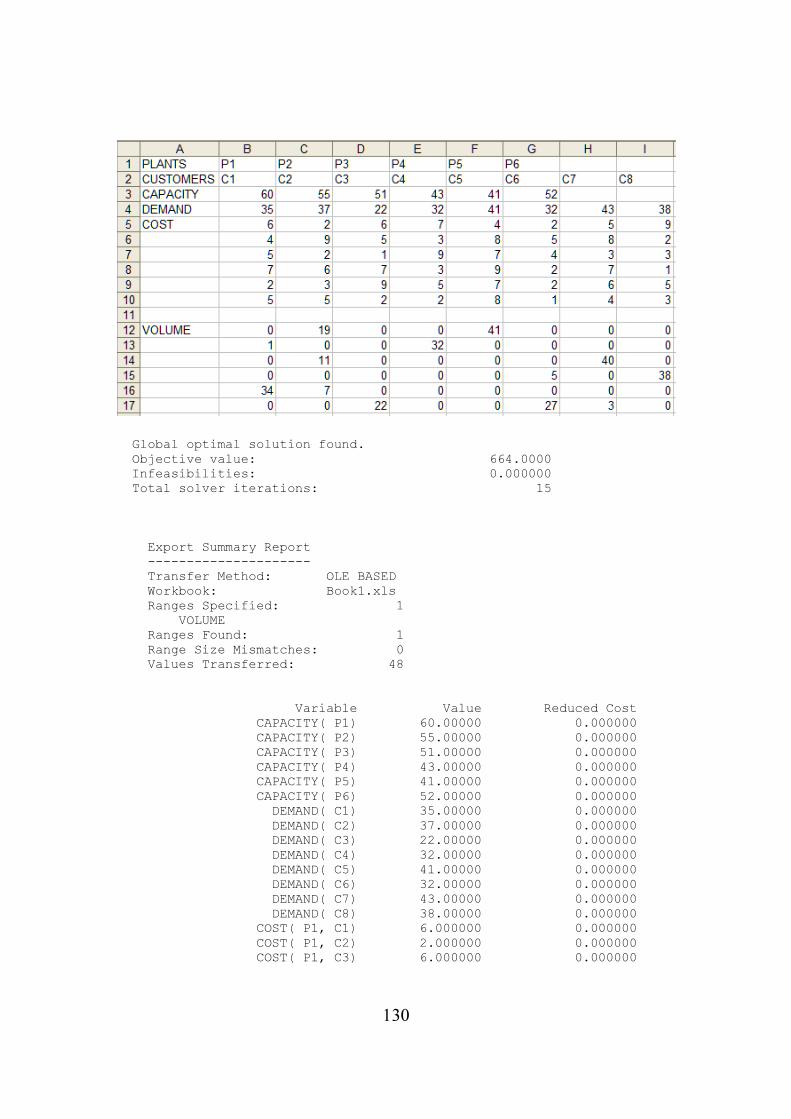
130
Global optimal solution found. Objective value: 664.0000 Infeasibilities: 0.000000 Total solver iterations: 15 Export Summary Report --------------------- Transfer Method: OLE BASED Workbook: Book1.xls Ranges Specified: 1 VOLUME Ranges Found: 1 Range Size Mismatches: 0 Values Transferred: 48 Variable Value Reduced Cost CAPACITY( P1) 60.00000 0.000000 CAPACITY( P2) 55.00000 0.000000 CAPACITY( P3) 51.00000 0.000000 CAPACITY( P4) 43.00000 0.000000 CAPACITY( P5) 41.00000 0.000000 CAPACITY( P6) 52.00000 0.000000 DEMAND( C1) 35.00000 0.000000 DEMAND( C2) 37.00000 0.000000 DEMAND( C3) 22.00000 0.000000 DEMAND( C4) 32.00000 0.000000 DEMAND( C5) 41.00000 0.000000 DEMAND( C6) 32.00000 0.000000 DEMAND( C7) 43.00000 0.000000 DEMAND( C8) 38.00000 0.000000 COST( P1, C1) 6.000000 0.000000 COST( P1, C2) 2.000000 0.000000 COST( P1, C3) 6.000000 0.000000
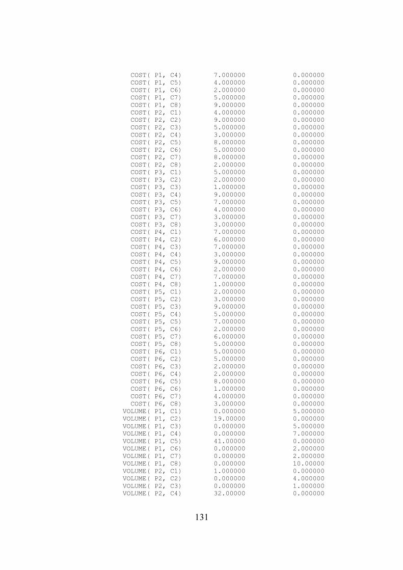
131
COST( P1, C4) 7.000000 0.000000 COST( P1, C5) 4.000000 0.000000 COST( P1, C6) 2.000000 0.000000 COST( P1, C7) 5.000000 0.000000 COST( P1, C8) 9.000000 0.000000 COST( P2, C1) 4.000000 0.000000 COST( P2, C2) 9.000000 0.000000 COST( P2, C3) 5.000000 0.000000 COST( P2, C4) 3.000000 0.000000 COST( P2, C5) 8.000000 0.000000 COST( P2, C6) 5.000000 0.000000 COST( P2, C7) 8.000000 0.000000 COST( P2, C8) 2.000000 0.000000 COST( P3, C1) 5.000000 0.000000 COST( P3, C2) 2.000000 0.000000 COST( P3, C3) 1.000000 0.000000 COST( P3, C4) 9.000000 0.000000 COST( P3, C5) 7.000000 0.000000 COST( P3, C6) 4.000000 0.000000 COST( P3, C7) 3.000000 0.000000 COST( P3, C8) 3.000000 0.000000 COST( P4, C1) 7.000000 0.000000 COST( P4, C2) 6.000000 0.000000 COST( P4, C3) 7.000000 0.000000 COST( P4, C4) 3.000000 0.000000 COST( P4, C5) 9.000000 0.000000 COST( P4, C6) 2.000000 0.000000 COST( P4, C7) 7.000000 0.000000 COST( P4, C8) 1.000000 0.000000 COST( P5, C1) 2.000000 0.000000 COST( P5, C2) 3.000000 0.000000 COST( P5, C3) 9.000000 0.000000 COST( P5, C4) 5.000000 0.000000 COST( P5, C5) 7.000000 0.000000 COST( P5, C6) 2.000000 0.000000 COST( P5, C7) 6.000000 0.000000 COST( P5, C8) 5.000000 0.000000 COST( P6, C1) 5.000000 0.000000 COST( P6, C2) 5.000000 0.000000 COST( P6, C3) 2.000000 0.000000 COST( P6, C4) 2.000000 0.000000 COST( P6, C5) 8.000000 0.000000 COST( P6, C6) 1.000000 0.000000 COST( P6, C7) 4.000000 0.000000 COST( P6, C8) 3.000000 0.000000 VOLUME( P1, C1) 0.000000 5.000000 VOLUME( P1, C2) 19.00000 0.000000 VOLUME( P1, C3) 0.000000 5.000000 VOLUME( P1, C4) 0.000000 7.000000 VOLUME( P1, C5) 41.00000 0.000000 VOLUME( P1, C6) 0.000000 2.000000 VOLUME( P1, C7) 0.000000 2.000000 VOLUME( P1, C8) 0.000000 10.00000 VOLUME( P2, C1) 1.000000 0.000000 VOLUME( P2, C2) 0.000000 4.000000 VOLUME( P2, C3) 0.000000 1.000000 VOLUME( P2, C4) 32.00000 0.000000
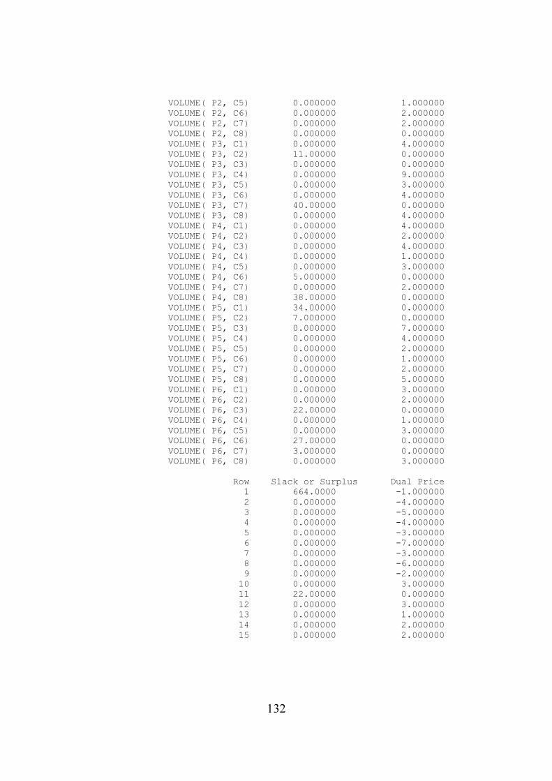
132
VOLUME( P2, C5) 0.000000 1.000000 VOLUME( P2, C6) 0.000000 2.000000 VOLUME( P2, C7) 0.000000 2.000000 VOLUME( P2, C8) 0.000000 0.000000 VOLUME( P3, C1) 0.000000 4.000000 VOLUME( P3, C2) 11.00000 0.000000 VOLUME( P3, C3) 0.000000 0.000000 VOLUME( P3, C4) 0.000000 9.000000 VOLUME( P3, C5) 0.000000 3.000000 VOLUME( P3, C6) 0.000000 4.000000 VOLUME( P3, C7) 40.00000 0.000000 VOLUME( P3, C8) 0.000000 4.000000 VOLUME( P4, C1) 0.000000 4.000000 VOLUME( P4, C2) 0.000000 2.000000 VOLUME( P4, C3) 0.000000 4.000000 VOLUME( P4, C4) 0.000000 1.000000 VOLUME( P4, C5) 0.000000 3.000000 VOLUME( P4, C6) 5.000000 0.000000 VOLUME( P4, C7) 0.000000 2.000000 VOLUME( P4, C8) 38.00000 0.000000 VOLUME( P5, C1) 34.00000 0.000000 VOLUME( P5, C2) 7.000000 0.000000 VOLUME( P5, C3) 0.000000 7.000000 VOLUME( P5, C4) 0.000000 4.000000 VOLUME( P5, C5) 0.000000 2.000000 VOLUME( P5, C6) 0.000000 1.000000 VOLUME( P5, C7) 0.000000 2.000000 VOLUME( P5, C8) 0.000000 5.000000 VOLUME( P6, C1) 0.000000 3.000000 VOLUME( P6, C2) 0.000000 2.000000 VOLUME( P6, C3) 22.00000 0.000000 VOLUME( P6, C4) 0.000000 1.000000 VOLUME( P6, C5) 0.000000 3.000000 VOLUME( P6, C6) 27.00000 0.000000 VOLUME( P6, C7) 3.000000 0.000000 VOLUME( P6, C8) 0.000000 3.000000 Row Slack or Surplus Dual Price 1 664.0000 -1.000000 2 0.000000 -4.000000 3 0.000000 -5.000000 4 0.000000 -4.000000 5 0.000000 -3.000000 6 0.000000 -7.000000 7 0.000000 -3.000000 8 0.000000 -6.000000 9 0.000000 -2.000000 10 0.000000 3.000000 11 22.00000 0.000000 12 0.000000 3.000000 13 0.000000 1.000000 14 0.000000 2.000000 15 0.000000 2.000000
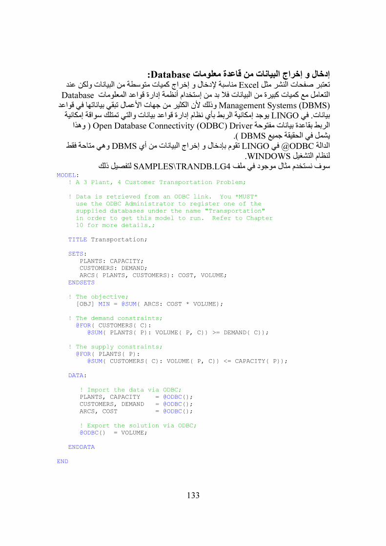
133
:Databaseإدخال و إخراج البيانات من قاعدة معلومات
مناسبة إلدخال و إخراج كميات متوسطة من البيانات ولكن عند Excelتعتبر صفحات النشر مثل Databaseالتعامل مع كميات كبيرة من البيانات فال بد من إستخدام أنظمة إدارة قواعد المعلومات
Management Systems (DBMS) ن الكثير من جهات األعمال تبقي بياناتها في قواعد وذلك أليوجد إمكانية الربط بأي نظام إدارة قواعد بيانات والتي تمتلك سواقة إمكانية LINGOبيانات. في
( وهذا Open Database Connectivity (ODBC) Driverالربط بقاعدة بيانات مفتوحة ). DBMSيشمل في الحقيقة جميع
وهي متاحة فقط DBMSتقوم بإدخال و إخراج البيانات من أي LINGOفي ODBC@الدالة .WINDOWSلنظام التشغيل
لتفصيل ذلك SAMPLES\TRANDB.LG4سوف نستخدم مثال موجود في ملف MODEL: ! A 3 Plant, 4 Customer Transportation Problem; ! Data is retrieved from an ODBC link. You *MUST* use the ODBC Administrator to register one of the supplied databases under the name "Transportation" in order to get this model to run. Refer to Chapter 10 for more details.; TITLE Transportation; SETS: PLANTS: CAPACITY; CUSTOMERS: DEMAND; ARCS( PLANTS, CUSTOMERS): COST, VOLUME; ENDSETS ! The objective; [OBJ] MIN = @SUM( ARCS: COST * VOLUME); ! The demand constraints; @FOR( CUSTOMERS( C): @SUM( PLANTS( P): VOLUME( P, C)) >= DEMAND( C)); ! The supply constraints; @FOR( PLANTS( P): @SUM( CUSTOMERS( C): VOLUME( P, C)) <= CAPACITY( P)); DATA: ! Import the data via ODBC; PLANTS, CAPACITY = @ODBC(); CUSTOMERS, DEMAND = @ODBC(); ARCS, COST = @ODBC(); ! Export the solution via ODBC; @ODBC() = VOLUME; ENDDATA END
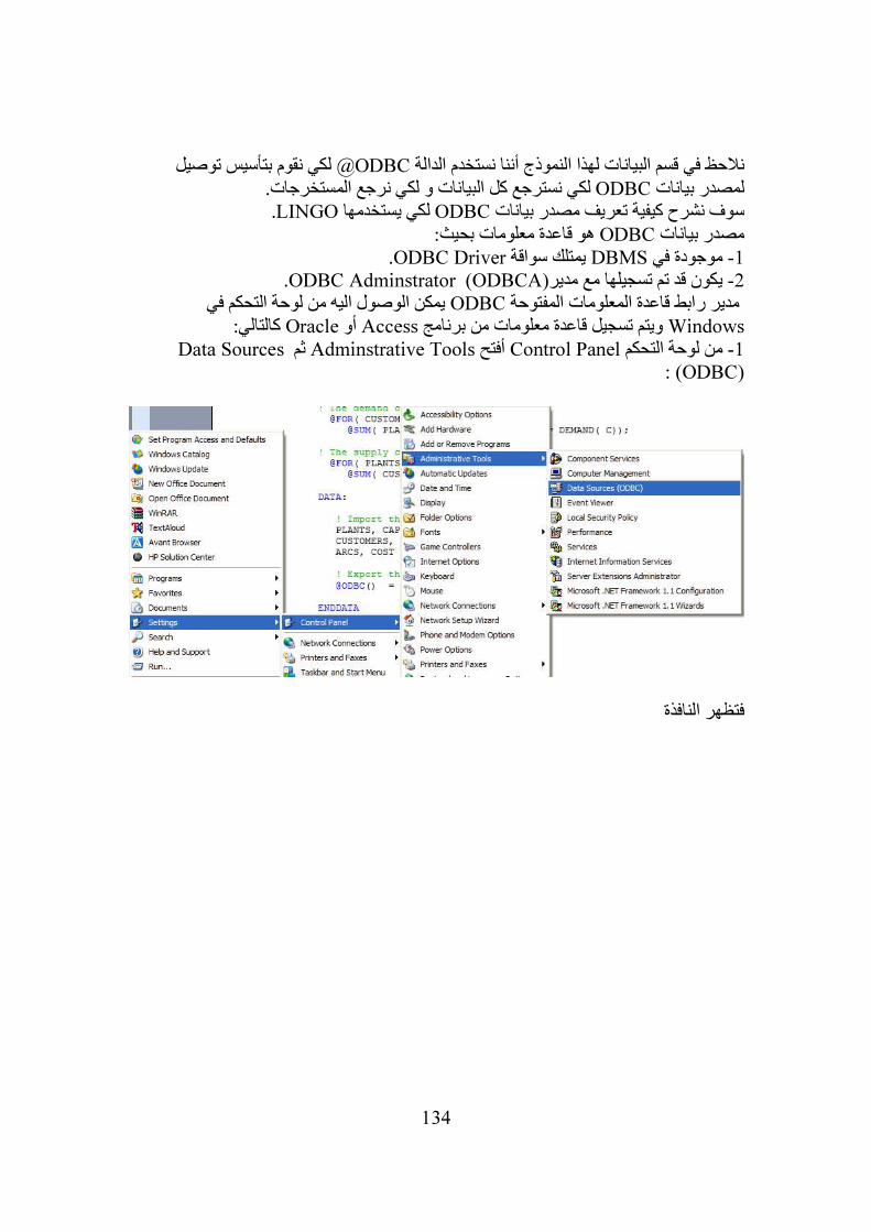
134
لكي نقوم بتأسيس توصيل ODBC@نالحظ في قسم البيانات لهذا النموذج أننا نستخدم الدالة لكي نسترجع كل البيانات و لكي نرجع المستخرجات. ODBCلمصدر بيانات
.LINGOلكي يستخدمها ODBCسوف نشرح كيفية تعريف مصدر بيانات هو قاعدة معلومات بحيث: ODBCمصدر بيانات
.ODBC Driverيمتلك سواقة DBMS موجودة في -1 . ODBC Adminstrator (ODBCA) يكون قد تم تسجيلها مع مدير -2يمكن الوصول اليه من لوحة التحكم في ODBCمدير رابط قاعدة المعلومات المفتوحة
Windows ويتم تسجيل قاعدة معلومات من برنامجAccess أوOracle :كالتالي Data Sourcesثم Adminstrative Toolsأفتح Control Panelمن لوحة التحكم -1
(ODBC) :
فتظهر النافذة
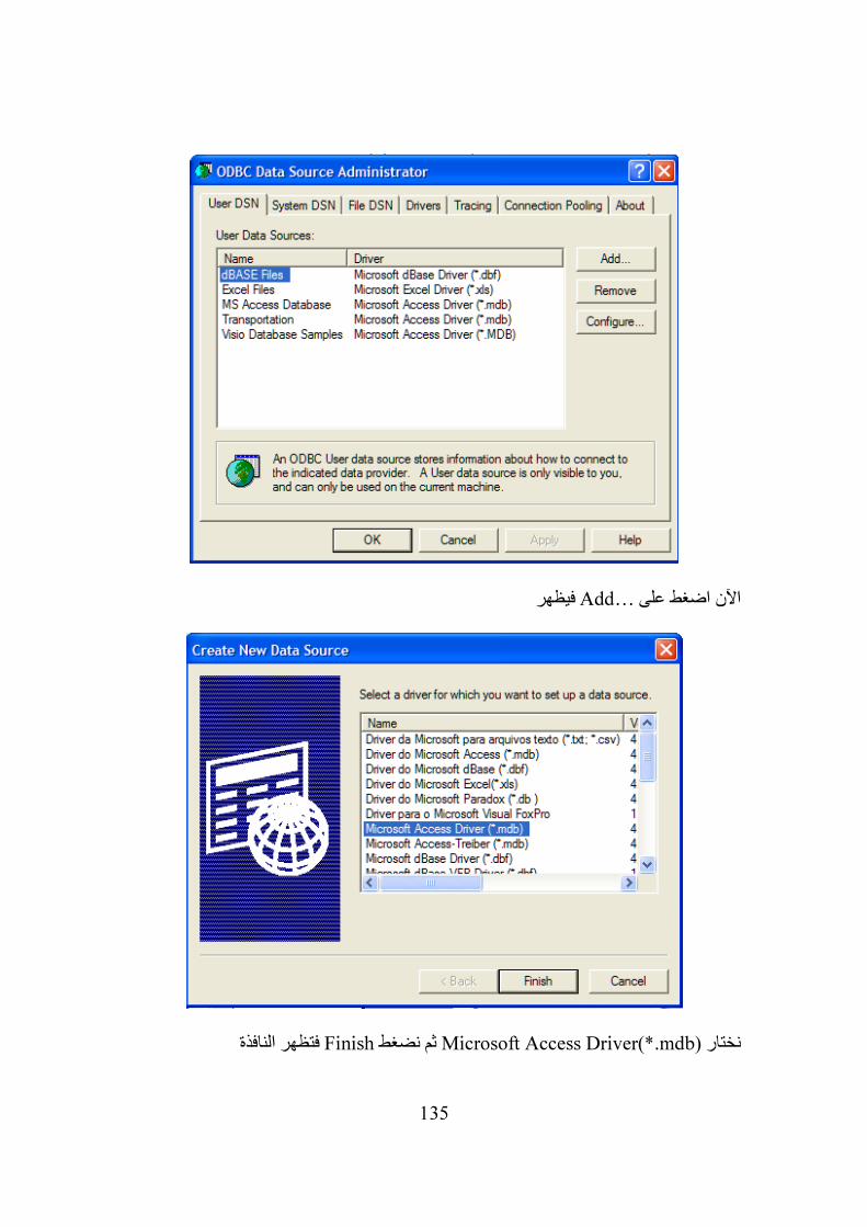
135
فيظهر …Addاآلن اضغط على
فتظهر النافذة Finishثم نضغط Microsoft Access Driver(*.mdb)نختار
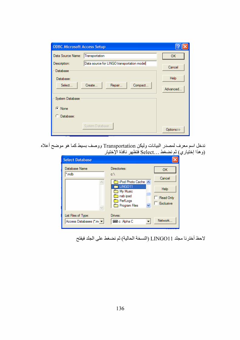
136
ه ووصف بسيط كما هو موضح أعال Transportationندخل اسم معرف لمصدر البيانات وليكن فتظهر نافذة اإلختيار …Select(وهذا إختياري) ثم نضغط
(النسخة الحالية) ثم نضغط على الجلد فيفتح LINGO11الحظ أخترنا مجلد
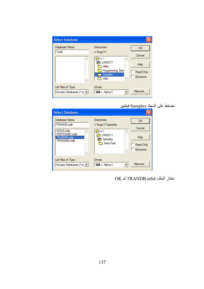
137
فيظهر Samplesنضغط على المجلد
OKثم TRANDB.mbdنختار الملف
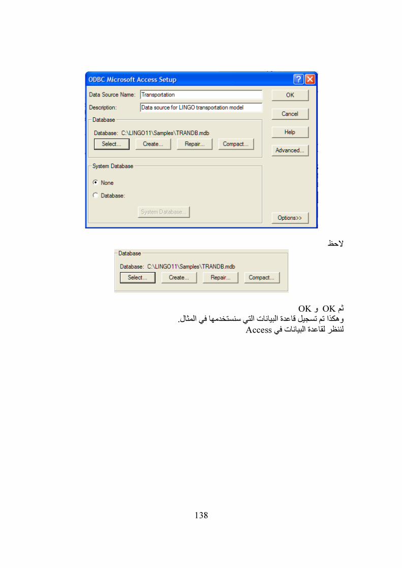
138
الحظ
OKو OKثم خدمها في المثال.وهكذا تم تسجيل قاعدة البيانات التي سنست
Accessلننظر لقاعدة البيانات في
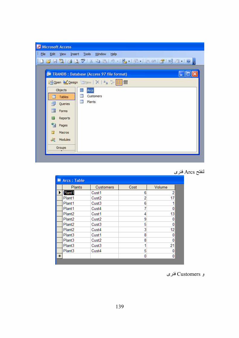
139
فنرى Arcsلنفتح
فنرى Customersو
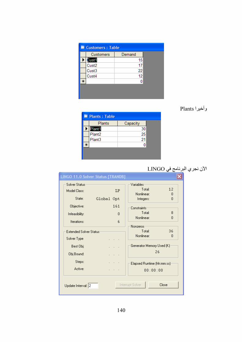
140
Plantsوأخيرا
LINGOاآلن نجري البرنامج في
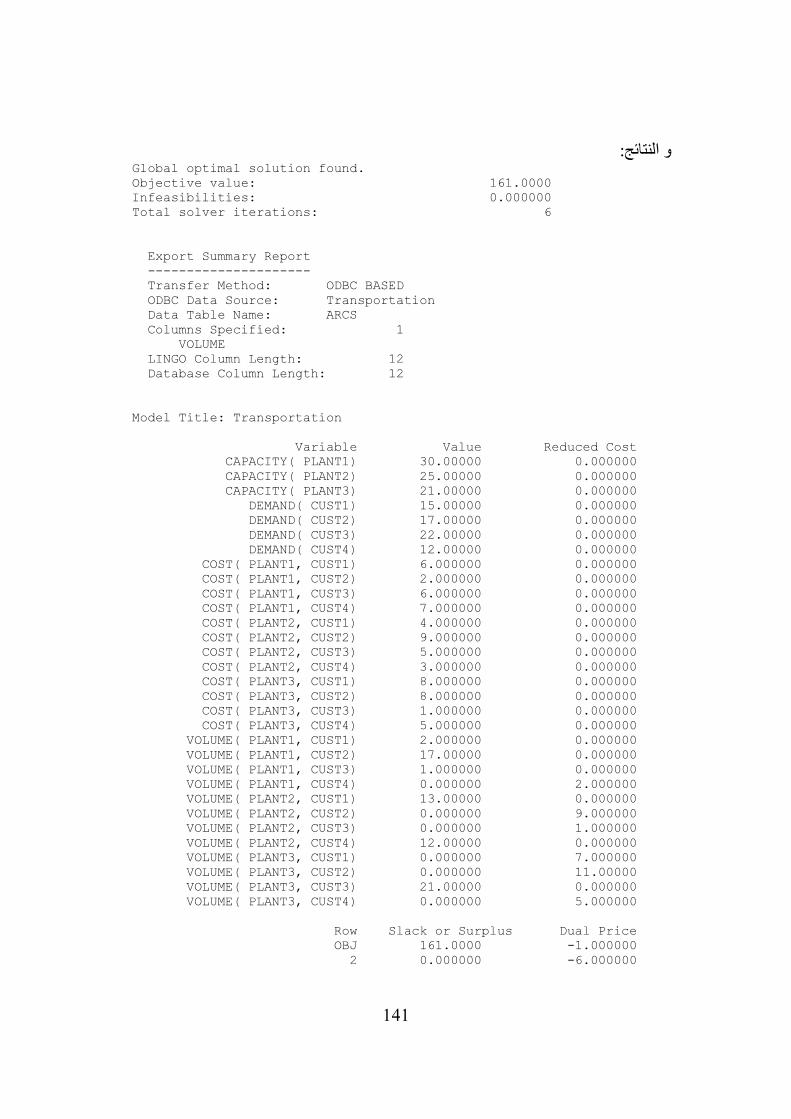
141
و النتائج: Global optimal solution found. Objective value: 161.0000 Infeasibilities: 0.000000 Total solver iterations: 6 Export Summary Report --------------------- Transfer Method: ODBC BASED ODBC Data Source: Transportation Data Table Name: ARCS Columns Specified: 1 VOLUME LINGO Column Length: 12 Database Column Length: 12 Model Title: Transportation Variable Value Reduced Cost CAPACITY( PLANT1) 30.00000 0.000000 CAPACITY( PLANT2) 25.00000 0.000000 CAPACITY( PLANT3) 21.00000 0.000000 DEMAND( CUST1) 15.00000 0.000000 DEMAND( CUST2) 17.00000 0.000000 DEMAND( CUST3) 22.00000 0.000000 DEMAND( CUST4) 12.00000 0.000000 COST( PLANT1, CUST1) 6.000000 0.000000 COST( PLANT1, CUST2) 2.000000 0.000000 COST( PLANT1, CUST3) 6.000000 0.000000 COST( PLANT1, CUST4) 7.000000 0.000000 COST( PLANT2, CUST1) 4.000000 0.000000 COST( PLANT2, CUST2) 9.000000 0.000000 COST( PLANT2, CUST3) 5.000000 0.000000 COST( PLANT2, CUST4) 3.000000 0.000000 COST( PLANT3, CUST1) 8.000000 0.000000 COST( PLANT3, CUST2) 8.000000 0.000000 COST( PLANT3, CUST3) 1.000000 0.000000 COST( PLANT3, CUST4) 5.000000 0.000000 VOLUME( PLANT1, CUST1) 2.000000 0.000000 VOLUME( PLANT1, CUST2) 17.00000 0.000000 VOLUME( PLANT1, CUST3) 1.000000 0.000000 VOLUME( PLANT1, CUST4) 0.000000 2.000000 VOLUME( PLANT2, CUST1) 13.00000 0.000000 VOLUME( PLANT2, CUST2) 0.000000 9.000000 VOLUME( PLANT2, CUST3) 0.000000 1.000000 VOLUME( PLANT2, CUST4) 12.00000 0.000000 VOLUME( PLANT3, CUST1) 0.000000 7.000000 VOLUME( PLANT3, CUST2) 0.000000 11.00000 VOLUME( PLANT3, CUST3) 21.00000 0.000000 VOLUME( PLANT3, CUST4) 0.000000 5.000000 Row Slack or Surplus Dual Price OBJ 161.0000 -1.000000 2 0.000000 -6.000000
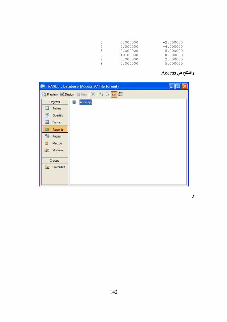
142
3 0.000000 -2.000000 4 0.000000 -6.000000 5 0.000000 -5.000000 6 10.00000 0.000000 7 0.000000 2.000000 8 0.000000 5.000000
Accessوالنتئج في
و
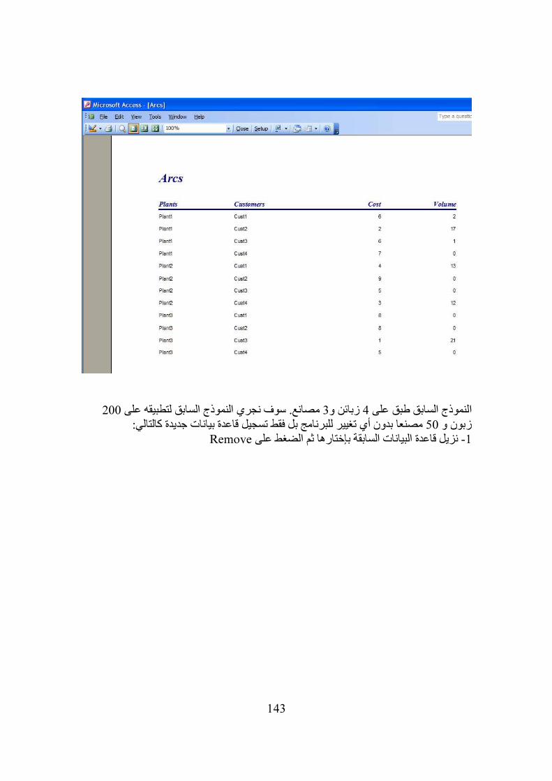
143
200مصانع. سوف نجري النموذج السابق لتطبيقه على 3زبائن و 4النموذج السابق طبق على مصنعا بدون أي تغيير للبرنامج بل فقط تسجيل قاعدة بيانات جديدة كالتالي: 50زبون و
Removeنزيل قاعدة البيانات السابقة بإختارها ثم الضغط على -1
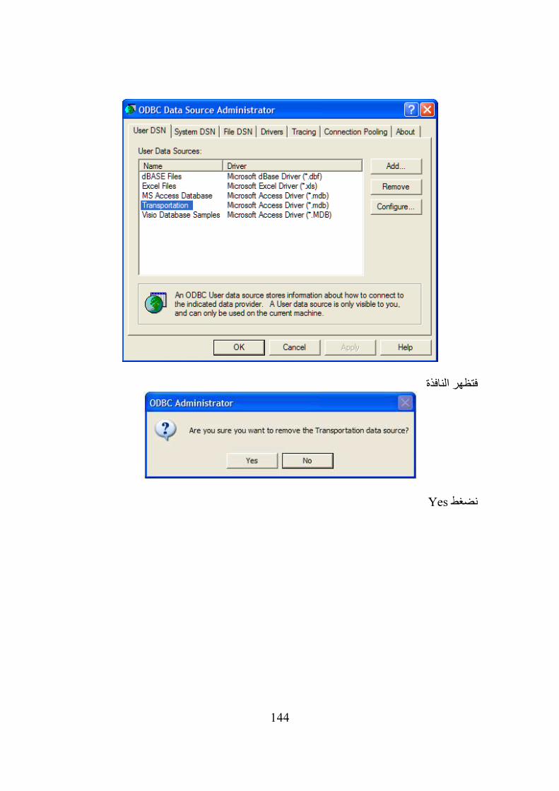
144
فتظهر النافذة
Yesنضغط
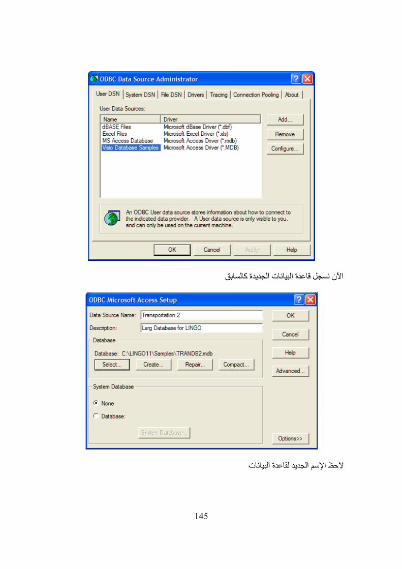
145
اآلن نسجل قاعدة البيانات الجديدة كالسابق
الحظ اإلسم الجديد لقاعدة البيانات
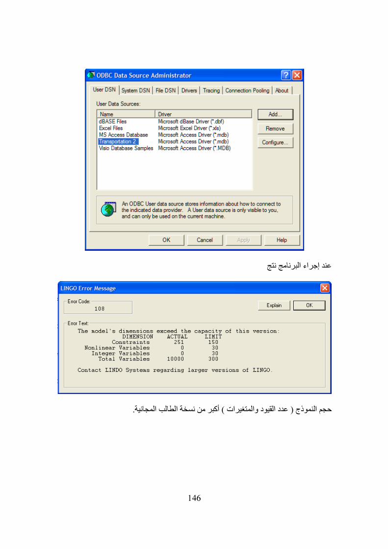
146
عند إجراء البرنامج نتج
حجم النموذج ( عدد القيود والمتغيرات ) أكبر من نسخة الطالب المجانية.

147
:Accessقاعدة البيانات في
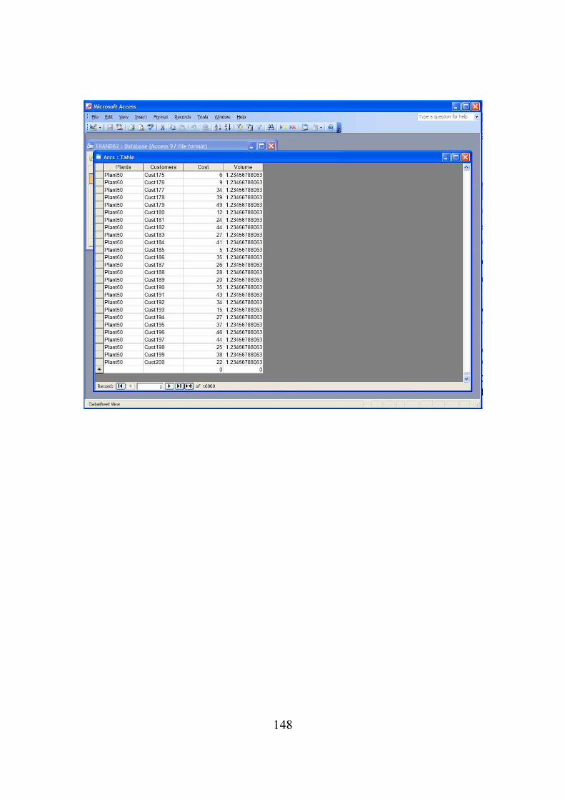
148
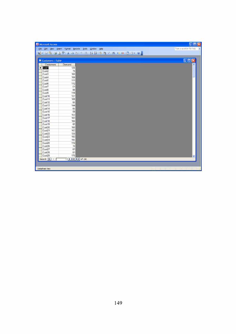
149
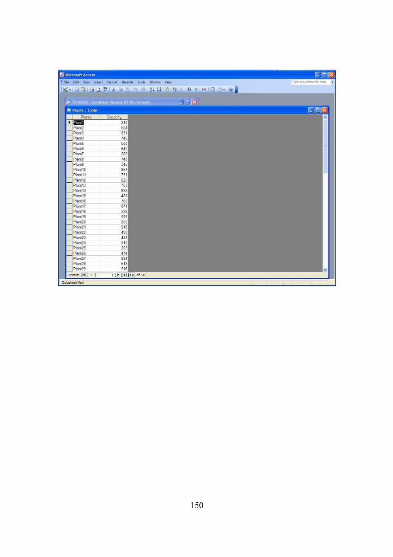
150

151
الفصل الخامس
:Rية بإستخدام حسابطرق
.Rلكي تطلع على مقدمة للغة النمذجة الرياضية 144مالحظة: أنظر للملحق صفحة
ف دوالتعري -1
Create a function from a formula
لتعريف دوال رياضية ولها التركيب التالي: makeFunتستخدم الدالة
makeFun(object, ...)
والتي تتكفل var = valهي شيئ لتوليد الدالة منه. الـ ... حجج إضافية على شكل objectالحجة
بالقيم اإلفتراضية لمدخالت الدلة.
Examples
library(mosaic)
f <- makeFun( sin(x^2 * b) ~ x & y & a); f
g <- makeFun( sin(x^2 * b) ~ x & y & a, a=2 ); g
h <- makeFun( a * sin(x^2 * b) ~ b & y, a=2, y=3); h
model <- lm(wage ~ poly(exper,degree=2), data=CPS85)
fit <- makeFun(model)
xyplot(wage ~ exper, data=CPS85)
plotFun(fit(exper) ~ exper, add=TRUE)
model <- glm(wage ~ poly(exper,degree=2), data=CPS85,
family=gaussian)
fit <- makeFun(model)
xyplot(wage ~ exper, data=CPS85)
plotFun(fit(exper) ~ exper, add=TRUE)

152
model <- nls( wage ~ A + B * exper + C * exper^2,
data=CPS85, start=list(A=1,B=1,C=1) )
fit <- makeFun(model)
xyplot(wage ~ exper, data=CPS85)
plotFun(fit(exper) ~ exper, add=TRUE)
المشتقات العددية -2
Numerical Derivatives
تكون أو تعطي المشتقة العددية لتعبير رياضي. numDالدالة
التالي:ولها التركيب
numD(formula, ..., .hstep = NULL, add.h.control = FALSE)
setInterval(C, wrt, h)
setCorners(C, var1, var2, h)
dfdx(.function, .wrt, .hstep)
d2fdxdy(.function, .var1, .var2, .hstep)
d2fdx2(.function, .wrt, .hstep)
numerical.first.partial(f, wrt, h, av)
numerical.second.partial(f, wrt, h, av)
numerical.mixed.partial(f, var1, var2, h, av)
الحجج:
153
Arguments
تعبير رياضي formula
معالم إضافية وغالبا ماتكون القيم اإلفتراضية للمعالم الرياضية. ...
الخطوة العددية للفروق المحدودة. .hstep
تهي الدالة الناتجة ليكون لها خطوة عددية لضمان التقارب. add.h.control
Examples
library(mosaic)
g = numD( a*x^2 + x*y ~ x, a=1)
g(x=2,y=10)
gg = numD( a*x^2 + x*y ~ x&x, a=1)
gg(x=2,y=10)
ggg = numD( a*x^2 + x*y ~ x&y, a=1)
ggg(x=2,y=10)
h = numD( g(x=x,y=y,a=a) ~ y, a=1)
h(x=2,y=10)
f = numD( sin(x)~x, add.h.control=TRUE)
plotFun( f(3,.hstep=h)~h, hlim=range(.00000001,.000001))
ladd( panel.abline(cos(3),0))
154
التفاضل العددي -3
Numerical Differentiation
مستخدمة تقريب الفروق المحدودة 4وحتى 1تعطي التفاضل العددي من الرتب fderivالدالة
Finite Difference.
ولها التركيب التالي:
fderiv(f, x, n = 1, h = 0, method="central", ...)
الحجج:
الدالة المطلوب تفاضلها. f
النقطة او النقاط التي سيتم عندها التفاضل. x
. 4وحتى 1درجة التفاضل وهي من n
(يجعل البرنامج يختارها ذاتيا). 0والقيمة اإفتراضية حجم الخطوة طول او h
واحد من: method
“central”, “forward”, or “backward”.
حجج إضافية وقيم إفتراضية. ...
Examples
library(pracma)
## Not run:
f <- sin
xs <- seq(-pi, pi, length.out = 100)
ys <- f(xs)
y1 <- fderiv(f, xs, n = 1, method = "backward")
y2 <- fderiv(f, xs, n = 2, method = "backward")
155
y3 <- fderiv(f, xs, n = 3, method = "backward")
y4 <- fderiv(f, xs, n = 4, method = "backward")
plot(xs, ys, type = "l", col = "gray", lwd = 2,
xlab = "", ylab = "", main = "Sinus and its
Derivatives")
lines(xs, y1, col=1, lty=2)
lines(xs, y2, col=2, lty=3)
lines(xs, y3, col=3, lty=4)
lines(xs, y4, col=4, lty=5)
grid()
## End(Not run)
التكامل العددي -4
Numerical integration
طرق التكامل العددي بإستخدام:
1- Euler
2- Runge-Kutta 4th order
3- Monte Carlo
4- RK4 with discontinuities
5- Ramos method.
و لهم التراكيب التالية:
euler(x0, t, f, p, dt)
RK4(x0, t, f, p, dt)
rnum(x0, t, f, p, dt, n)
RK4D(x0, t, f, p, dt, g, tz)
ramos(x0, t, f, p, dt)
في النموذج Xتستخدم فقط لألغراض التعليمية (التوضيحية) وتستخدم لكي نوجد eulerالدالة
dX/dt = f(t,p,X)

156
لحل النموذج 4ذات الرتبة RKتستخدم طريقة RK4الدالة
dX/dt = f(t,p,X)
عدديا.
.eulerوم على نفس مبدأ تشبة أو تق rnumالدلة
تتعامل مع اإلنقطاعات أو الفجوات في الدالة المطلوب تكاملها. RK4Dالدالة
تستخدم طريقة رامس للتكامل. ramosالدالة
الحجج:
الشرط األولي x0
initial condition
األزمنة لإلخراج t
times for output
ادلة التفاضلية العادية دالة النموذج ( الطرف األيسر للمع f
right hand side of ODE
معالم. p
الخطوات الزمنية. dt
عدد اإلنجازات. n
دالة اإلنقطاعات. g
أزمنة اإلنقطاعات. tz
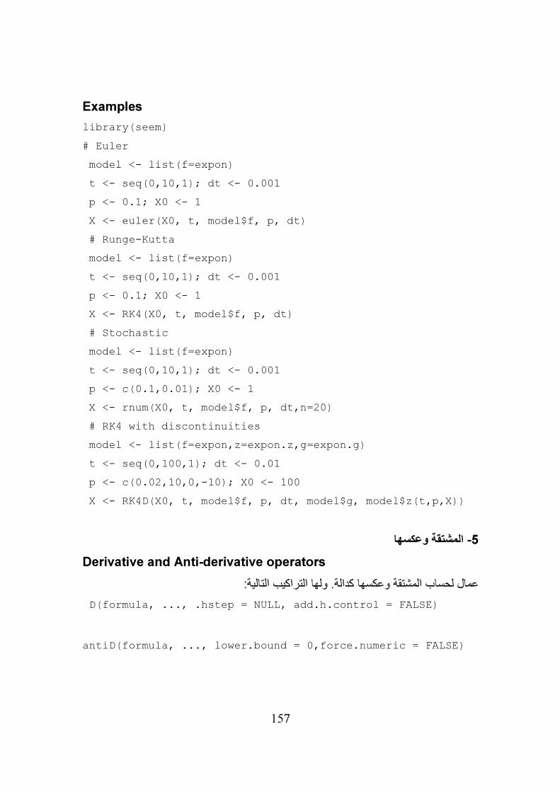
157
Examples
library(seem)
# Euler
model <- list(f=expon)
t <- seq(0,10,1); dt <- 0.001
p <- 0.1; X0 <- 1
X <- euler(X0, t, model$f, p, dt)
# Runge-Kutta
model <- list(f=expon)
t <- seq(0,10,1); dt <- 0.001
p <- 0.1; X0 <- 1
X <- RK4(X0, t, model$f, p, dt)
# Stochastic
model <- list(f=expon)
t <- seq(0,10,1); dt <- 0.001
p <- c(0.1,0.01); X0 <- 1
X <- rnum(X0, t, model$f, p, dt,n=20)
# RK4 with discontinuities
model <- list(f=expon,z=expon.z,g=expon.g)
t <- seq(0,100,1); dt <- 0.01
p <- c(0.02,10,0,-10); X0 <- 100
X <- RK4D(X0, t, model$f, p, dt, model$g, model$z(t,p,X))
المشتقة وعكسها -5
Derivative and Anti-derivative operators
عمال لحساب المشتقة وعكسها كدالة. ولها التراكيب التالية:
D(formula, ..., .hstep = NULL, add.h.control = FALSE)
antiD(formula, ..., lower.bound = 0,force.numeric = FALSE)

158
makeAntiDfun(.function, .wrt, from,.tol =
.Machine$double.eps^0.25)
numerical.integration(f, wrt, av, args, vi.from, ciName =
"C", .tol)
الحجج:
صيغة. formula
القيم اإلفتراضية. ...
المسافات األفقية بين النقاط المستخدمة لحساب المشتقات العددية. .hstep
المشتقة العددية.قيمة منطقية تستخدم لحساب add.h.control
الحد األدنى لحساب المشتقة العددية. lower.bound
force.numeric إذا كانTRUE يجرى تكامل عددي حتى لو كان يوجد تكامل رمزي
symbolic integral.
الدالة المراد تكاملها. .function
صف من الحروف يسمي متغير التكامل. .wrt
اضية للحد األدنى لمجال التكامل.القيمة اإلفتر from
دالة. f
صف حرفي يسمي المتغير. wrt
قائمة من الحجج الممررة للدالة. av
القيم اإلفتراضية للمعالم إذا وجدت. args
الحد العددي المسموح للخطأ. .tol
Examples
library(mosaic)
D(sin(t) ~ t)
D(A*sin(t) ~ t )
D(A*sin(2*pi*t/P) ~ t, A=2, P=10) # default values for
parameters.
159
f <- D(A*x^3 ~ x + x, A=1) # 2nd order partial -- note,
it's a function of x
f(x=2)
f(x=2,A=10) # override default value of parameter A
g <- D(f(x=t, A=1)^2 ~ t) # note: it's a function of t
g(t=1)
gg <- D(f(x=t, A=B)^2 ~ t, B=10) # note: it's a function
of t and B
gg(t=1)
gg(t=1, B=100)
f <- makeFun(x^2~x)
D(f(cos(z))~z) #will look in user functions also
antiD( a*x^2 ~ x)
antiD( A/x~x )
F <- antiD( A*exp(-k*t^2 ) ~ t, A=1, k=0.1)
F(t=Inf)
one = makeFun(1~x&y)
by.x = antiD( one(x=x, y=y) ~x)
by.xy = antiD(by.x(x=sqrt(1-y^2), y=y)~y)
4*by.xy(y=1) #area of quarter circle
المشتقات الرمزية -6
Symbolic Derivatives
تعطي المشتقات الرياضية لبعض التعابير. ولها الركيب التالي:
symbolicD(formula, ..., .order = NULL)
الحجج:
تعبير رياضي. formula
معالم إضافية وغالبا ما تكون القيم اإلفتراضية للمعالم الرياضية. ...
رقم يحدد درجة المشتقة لمتغير واحد. .order

160
Examples
library(mosaic)
symbolicD( a*x^2 ~ x)
symbolicD( a*x^2 ~ x&x)
symbolicD( a*sin(x)~x, .order=4)
symbolicD( a*x^2*y+b*y ~ x, a=10, b=100 )
رسم تعابير رياضية -7
Plotting mathematical expressions
لرسم تعابير رياضية لمتغير او اثنين ولها التركيب التالي: plotFunتستخدم الدالة
plotFun(object, ..., add = FALSE, xlim = NULL,
ylim = NULL, npts = NULL, ylab = NULL, xlab = NULL,
zlab = NULL, filled = TRUE, levels = NULL,
nlevels = 10, labels = TRUE, surface = FALSE,
groups = NULL, col.regions = topo.colors, type = "l",
alpha = NULL)
الحجج:
تعبير رياضي أو دالة لمتغير واحدة. object
add كان إذاTRUE .يضاف الرسم إلى رسم حالي
xlim .حدود المحور االفقي
ylim .حدود المحور العامودي
npts .عدد النقاط التي يتم رسمها
xlab .إسم المحور االفقي
ylab .إسم المحور العامودي
zlab إسم المحور الثالث للرسوم السطحيةsurface-plot.
col .لون الرسم
161
filled لمناطق في الرسم باللون.ملي ا
levels .مستويات الرسم لرسوم الكنتور
nlevels .عدد الكنتورات المرسومة
labels إذا كانتFALES .فال تسمى الكنتورات
surface .يرسم رسم سطحي بدل الرسم الكنتوري
col.regions .متجه من االلوان أو دالة
type .نوع الرسم
alpha (غير شفاف) أللوان الملئ. 1اف) إلى (شف 0عدد من
groups حجة التجميع لرسوم الشبكيةLattice graphics.
معالم إضافية. ...
Examples
library(mosaic)
plotFun( a*sin(x^2)~x, xlim=range(-5,5), a=2 )
plotFun( u^2 ~ u, ulim=c(-4,4) )
plotFun( y^2 ~ y, ylim=c(-2,20), y.lim=c(-4,4) )
plotFun( x^2 -3 ~ x, xlim=c(-4,4), grid=TRUE )
ladd( panel.abline(h=0,v=0,col='gray50') )
plotFun( (x^2 -3) * (x^2 > 3) ~ x, type='h', alpha=.1,
lwd=4, col='lightblue', add=TRUE )
plotFun( sin(x) ~ x,
groups=cut(x, findZeros(sin(x) ~ x, within=10)$x),
col=c('blue','green'), lty=2, lwd=3, xlim=c(-10,10) )
plotFun( sin(2*pi*x/P)*exp(-k*t)~x+t,k=2,P=.3)
f <- rfun( ~ u & v )
plotFun( f(u=u,v=v) ~ u & v, u.lim=range(-3,3),
v.lim=range(-3,3) )
plotFun( u^2 + v < 3 ~ u & v, add=TRUE, npts=200 )

162
model <- lm(wage ~ poly(exper,degree=2), data=CPS85)
fit <- makeFun(model)
xyplot(wage ~ exper, data=CPS85)
plotFun(fit(exper) ~ exper, add=TRUE, lwd=8)
plotFun(fit, add=TRUE, lwd=2, col='white')
plotFun( sin(k*x)~x, k=0.01 )

163
:Rحل مشاكل األمثلية بواسطة
في حل مشاكل Rف نستخدم ثالثة حزم رياضية إلستعراض مقدرات لغة النمذجة الرياضية سو
األمثلية. GNU Linear لعدة Rوهو واجة إستخدام في 'Package 'Rglpkأول هذه الحزم هي حزمة
Programing Kit للبرمجة الخطية المسماةGLPK وهي حزمة مجانية والتي تقوم بحل مشاكل اق في البرمجة خطية والبرمجة العددية والبرمجة المختلطة وغيرها.واسعة النط
وهي حزمة متوفرة مجانا لحل مشاكل البرمجة 'Package 'lpSolveالحزمة الثانية هي حزمة الخطية والعددية والمختلطة ومشاكل التخصيص والنقل وغيرها.
ل البرمجة الخطية ومشاكل ويستخدم لحل مشاك 'Package 'linprogالحزمة الثالثة هي حزمة .Simplex Algorithmاألمثلية بإستخدام خوارزم السمبلكس
وتستخدم كالتالي: Rglpkأوال: حزمة
Rglpk_solve_LP(obj, mat, dir, rhs, types = NULL, max = FALSE, bounds = NULL, verbose = FALSE)
حيث:
obj .متجة يحوي معامل دالة الهدف mat مصفوفة معامل القيود. متجه أو
dir متجة نصي وفيه إتجاهات القيود ويجب ان تكون ,"=<" ,"<" ,"=>" ,">"or "==". rhs .الطرف األيمن من القيود
types متجة يبين انواع متغيرات الهدف ويجب ان يكون"B" للثنائي و"C" للمستمر و"I" ."C"للصحيح والقيمة اإلفتراضية هي
max ية تعطي إتجاه األمثلية فالقيمة قيمة منطقTRUE تعني تعظيمmaximize دالة الهدف وFALSE تعني التصغيرminimize. bounds وقيمتها اإلفتراضيةNULL أو قائمة بعناصر علياupper ودنياlower تحوي فهارسindices و 0ن والحدود التابعة لها لمتغيرات الهدف القيمة اإلفتراضية لكل متغير هي بي∞.
verbose قيمة منطقية لكي نخبر الحاللsolver بأن يعطي مخرجات إضافية أو ال والقيمة .FALSEاإلفتراضية
المخرجات:
مع التالي: optimal solutionقائمة تحوي الحل األمثل solution الحل وهو متجه للعوامل المثلىoptimal coefficients.
objval .قيمة دالة الهدف عند الحل األمثل status إذا كان الحل أمثل. 0وهو عدد صحيح يعطي معلومات الحالة عن الحل ويعطي
وقيمة غير صفرية غير ذلك.
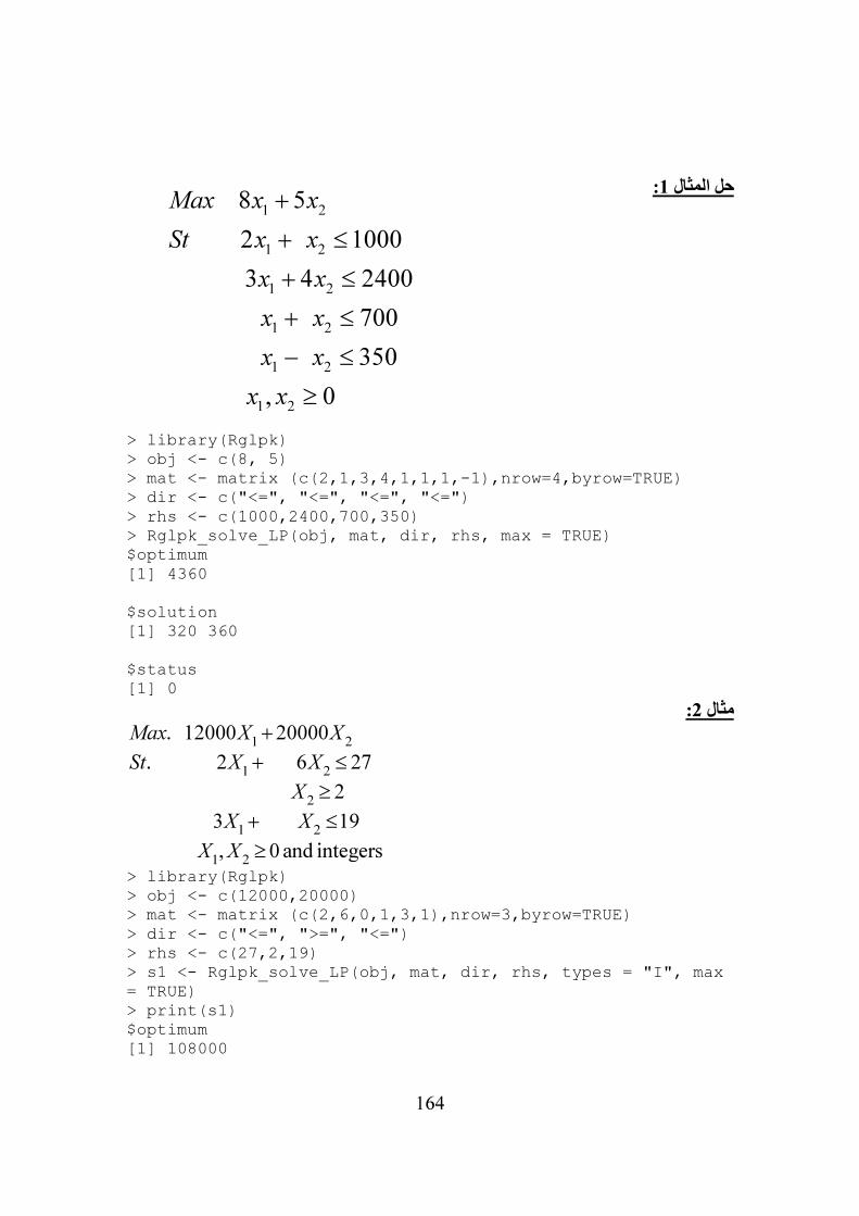
164
:1حل المثال
> library(Rglpk) > obj <- c(8, 5) > mat <- matrix (c(2,1,3,4,1,1,1,-1),nrow=4,byrow=TRUE) > dir <- c("<=", "<=", "<=", "<=") > rhs <- c(1000,2400,700,350) > Rglpk_solve_LP(obj, mat, dir, rhs, max = TRUE) $optimum [1] 4360 $solution [1] 320 360 $status [1] 0
:2مثال
1 2
1 2
2
1 2
1 2
. 12000 20000
. 2 6 27
2
3 19
, 0 and integers
Max X X
St X X
X
X X
X X
+
+ ≤
≥
+ ≤
≥
> library(Rglpk) > obj <- c(12000,20000) > mat <- matrix (c(2,6,0,1,3,1),nrow=3,byrow=TRUE) > dir <- c("<=", ">=", "<=") > rhs <- c(27,2,19) > s1 <- Rglpk_solve_LP(obj, mat, dir, rhs, types = "I", max = TRUE) > print(s1) $optimum [1] 108000
1 2
1 2
1 2
1 2
1 2
1 2
8 5
2 1000
3 4 2400
700
350
, 0
Max x x
St x x
x x
x x
x x
x x
+
+ ≤
+ ≤
+ ≤
− ≤
≥

165
$solution [1] 4 3 $status [1] 0 >
linprogة ثانيا الحل بإستخدام الحزم
لحل النظام: ,
, 0
minimize c x
subject to Ax b x
′
≤ ≥
وتستخدم كالتالي:
solveLP( cvec, bvec, Amat, maximum=FALSE, maxiter=1000, zero=1e-10, lpSolve=FALSE, verbose=FALSE )
حيث:
cvec المتجهc ويحويn .عنصر bvec المتجةb ويحويm .عنصر
Amat المصفوفةA بأبعادm x n. maximum .قيمة منطقية لتعظيم أو تصغير دالة الهدف والقيمة اإلفتراضية تصغير
maxiter .أقصى عدد للتكرار zero .تخبر البرنامج في ان يضع األرقام التي هي اصغر من هذا العدد مساوية للصفر
lpSolve قيمة منطقية إلخبار البرنامج إلستخدام الحزمة'lpSolve' ة اإلفتراضية ال.أو ال. القيم verbose قيمة منطقية إختيارية إلخبار البرنامج لطباعة النتائج المرحلية أو ال. والقيمة اإلفتراضية
ال.
:1حل مثال
> library( linprog ) > cvec <- c(8,5) > bvec <- c(1000,2400,700,350) > Amat <- rbind( c( 2, 1),c( 3,4 ),c( 1, 1 ), c( 1, -1 )) > res <- solveLP( cvec, bvec, Amat, TRUE ) > print.solveLP( res ) Results of Linear Programming / Linear Optimization
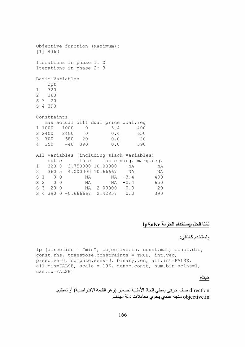
166
Objective function (Maximum): [1] 4360 Iterations in phase 1: 0 Iterations in phase 2: 3 Basic Variables opt 1 320 2 360 S 3 20 S 4 390 Constraints max actual diff dual price dual.reg 1 1000 1000 0 3.4 400 2 2400 2400 0 0.4 650 3 700 680 20 0.0 20 4 350 -40 390 0.0 390 All Variables (including slack variables) opt c min c max c marg. marg.reg. 1 320 8 3.750000 10.00000 NA NA 2 360 5 4.000000 10.66667 NA NA S 1 0 0 NA NA -3.4 400 S 2 0 0 NA NA -0.4 650 S 3 20 0 NA 2.00000 0.0 20 S 4 390 0 -0.666667 2.42857 0.0 390
lpSolveثالثا الحل بإستخدام الحزمة
وتستخدم كالتالي:
lp (direction = "min", objective.in, const.mat, const.dir, const.rhs, transpose.constraints = TRUE, int.vec, presolve=0, compute.sens=0, binary.vec, all.int=FALSE, all.bin=FALSE, scale = 196, dense.const, num.bin.solns=1, use.rw=FALSE)
حيث:
direction .صف حرفي يعطي إتجاة األمثلية تصغير (وهو القيمة اإلفتراضية) أو تعظيم objective.in .متجه عددي يحوي معامالت دالة الهدف

167
const.mat مصفوفة عددية لمعامالت القيود صف واحد لكل قيد وعمود واحد لكل متغير قرار ). transpose.constraints = FALSEي حالة (ماعدى ف
const.dir ) متجه من النصوص يعطي إتجاه القيد ويجب أن تكون أحد التالي"<" "<=" "=" "==" ">" ">="(. const.rhs .متجه من القيم العددية للجة اليمنى من القيود
transpose.constraints في العادة كل قيد يشغل سطر منconst.mat ه المصفوفة تحتاج وهذقبل تمريرها لخوارزم األمثلية. ولهذا في حالة مصفوفة قيود كبيرة جدا قد transposeإلى عكس
يكون من األفضل وضع القيود في المصفوفة عمود بعمود وفي هذه الحالة نضع transpose.constraints = FALSE.
int.vec متجه عددي يعطي مؤشراتindices وب أن تكون صحيحة.المتغيرات المطل presolve 0عدد القيمة اإلفتراضية له.
compute.sens أي ال. 0عدد لحساب الحساسية قيمته اإلفتراضية binary.vec متجه عددي يعطي مؤشراتindices .المتغيرات المطلوب أن تكون ثنائية
all.int راضية: قيمة منطقية. هل كل المتغيرات يجب أن تكون صحيحة؟ القيمة اإلفتFALSE. all.bin :قيمة منطقية. هل كل المتغيرات يجب أن تكون ثنائية؟ القيمة اإلفتراضيةFALSE.
scale و 196عدد صحيح لقيمة القياس (لجعل جميع القيم العددية بنفس القياس) القيمة اإلفتراضية لعدم تغيير القياس. 0
dense.const مرصوصةarray أعمدة. وتهمل في حال إعطاء قيمة كثيفة للقيود ذات ثالثةconst.mat .
num.bin.solns عدد صحيح. إذا كانall.bin = TRUE فإن المستخدم يستطيع طلب العدد المعطى من الحلول المثلى.
use.rw منطقي إذا كانTRUE وكانnum.bin.solns >1 .فهو يعطي كل حل على إنفراد
المخرجات: .lp.objectعن طريق النداء:
:1مثال
> library(lpSolve) > f.obj <- c(8, 5) > f.con <- matrix (c(2,1,3,4,1,1,1,-1),nrow=4,byrow=TRUE) > f.dir <- c("<=","<=","<=","<=") > f.rhs <- c(1000,2400,700,350) > s1 <- lp ("max", f.obj, f.con, f.dir, f.rhs) > lp ("max", f.obj, f.con, f.dir, f.rhs)$solution [1] 320 360 > print(s1) Success: the objective function is 4360 >
مثال:

168
1 2 3
1 2 3
1 2 3
: 9
. : 2 3 9
3 2 2 15
max x x x
s t x x x
x x x
+ +
+ + ≤
+ + ≤
> library(lpSolve) > f.obj <- c(1, 9, 3) > f.con <- matrix (c(1, 2, 3, 3, 2, 2), nrow=2, byrow=TRUE) > f.dir <- c("<=", "<=") > f.rhs <- c(9, 15) > lp ("max", f.obj, f.con, f.dir, f.rhs) Success: the objective function is 40.5 > lp ("max", f.obj, f.con, f.dir, f.rhs)$solution [1] 0.0 4.5 0.0
تحليل الحساسية:> lp ("max", f.obj, f.con, f.dir, f.rhs, compute.sens=TRUE)$sens.coef.from [1] -1e+30 2e+00 -1e+30 > lp ("max", f.obj, f.con, f.dir, f.rhs, compute.sens=TRUE)$sens.coef.to [1] 4.50e+00 1.00e+30 1.35e+01 > lp ("max", f.obj, f.con, f.dir, f.rhs, compute.sens=TRUE)$duals [1] 4.5 0.0 -3.5 0.0 -10.5 > lp ("max", f.obj, f.con, f.dir, f.rhs, compute.sens=TRUE)$duals.from [1] 0e+00 -1e+30 -1e+30 -1e+30 -6e+00 > lp ("max", f.obj, f.con, f.dir, f.rhs, compute.sens=TRUE)$duals.to [1] 1.5e+01 1.0e+30 3.0e+00 1.0e+30 3.0e+00
إعادة اإلجراء مع جعل جميع المتغيرات صحيحة:
> lp ("max", f.obj, f.con, f.dir, f.rhs, int.vec=1:3) Success: the objective function is 37 > lp ("max", f.obj, f.con, f.dir, f.rhs, int.vec=1:3)$solution [1] 1 4 0 > lp ("max", f.obj, f.con, f.dir, f.rhs, int.vec=1:3, compute.sens=TRUE)$duals [1] 1 0 0 7 0
البرمجة العددية لمشكلة تخصيص:

169
يستخدم األمر lp.assign (cost.mat, direction = "min", presolve = 0, compute.sens = 0)
حيث:
cost.mat مصفوفة التكلفة العنصرij هو تكلفة تخصيص المصدرi للمقصدj. direction يحوي إما 1وص ذا طول متجة نص"min" وهي القيمة اإلفتراضية أو"max". presolve .قيمة عددية وتوضع مساوية للصفر
compute.sens قيمة عددية وإفتراضيا تساوي الصفر وأي قيمة غير صفرية تؤدي لحساب الحساسية.
.lp.object مخرجات:
مثال:
مصفوفة التكلفة:2 7 7 1
7 7 2 9
7 3 8 8
2 2 10 2
> assign.costs <- matrix (c(2, 7, 7, 2, 7, 7, 3, 2, 7, 2, 8,10, 1, 9, 8, 2), 4, 4) > assign.costs [,1] [,2] [,3] [,4] [1,] 2 7 7 1 [2,] 7 7 2 9 [3,] 7 3 8 8 [4,] 2 2 10 2 > lp.assign (assign.costs)$solution [,1] [,2] [,3] [,4] [1,] 0 0 0 1 [2,] 0 0 1 0 [3,] 0 1 0 0 [4,] 1 0 0 0 >
شيئ. وهو قائمة تحوي التالي: lpشيئ وهو هيكل لـ LPيعطي lp.objectاألمر
direction .إتجاه األفضلية كما في المدخل

170
x.count .عدد متغيرات القرار في دالة الهدف objective .متجه معامالت دالة الهدف كما في المدخل
const.count .عدد القيود المدخلة constraint يود كما ادخلت.مصفوفة الق int.count .عدد المتغيرات الصحيحة
int.vec .متجه مؤشرات المتغيرات الصحيحة كما ادخلت objval .قيمة دالة الهدف عند األمثلية
solution .متجة المعامالت المثلى num.bin.solns .مؤشر عددي لعدد الحلول الناتجة
status اليوجد حل ممكن2= نجاح و 0مؤشر عددي =.
برمجة مشكلة نقل:
يستخدم األمر:lp.transport (cost.mat, direction="min", row.signs, row.rhs, col.signs, col.rhs, presolve=0, compute.sens=0, integers = 1:(nc*nr) )
حيث:
cost.mat مصفوفة التكلفة العنصرij هو تكلفة تخصيص المصدرi للمقصدj. direction يحوي إما 1نصوص ذا طول متجة"min" وهي القيمة اإلفتراضية أو"max".
row.signs :متجة من النصوص يعطى إتجاهات قيود األسطر وكل قيمة يجب أن تكون أحد التالي "<" "<=" "=" "==" ">" ">=".
row.rhs .متجة من القيم العددية للجهة اليمنى من قيود األسطر col.signs يعطى إتجاهات قيود األعمدة وكل قيمة يجب أن تكون أحد التالي:متجة من النصوص
"<" "<=" "=" "==" ">" ">=". col.rhs .متجة من القيم العددية للجهة اليمنى من قيود األعمدة
presolve 0عدد القيمة اإلفتراضية له. compute.sens أي ال. 0عدد لحساب الحساسية قيمته اإلفتراضية
integers من األعداد الصحيحة عنصره متجهi يعطي مؤشر المتغير الصحيح رقمi والذي طوله هو عدد المتغيرات الصحيحة. اقيمة اإلفتراضية جميع المتغيرات صحيحة.
.lp.object المخرجات:
مثال:
> library(lpSolve) > costs <- matrix(10000,8,5) > costs[4,1] <- costs[-4,5] <- 0 > costs[1,2] <- costs[2,3] <- costs[3,4] <- 7 > costs[1,3] <- costs[2,4] <- 7.7
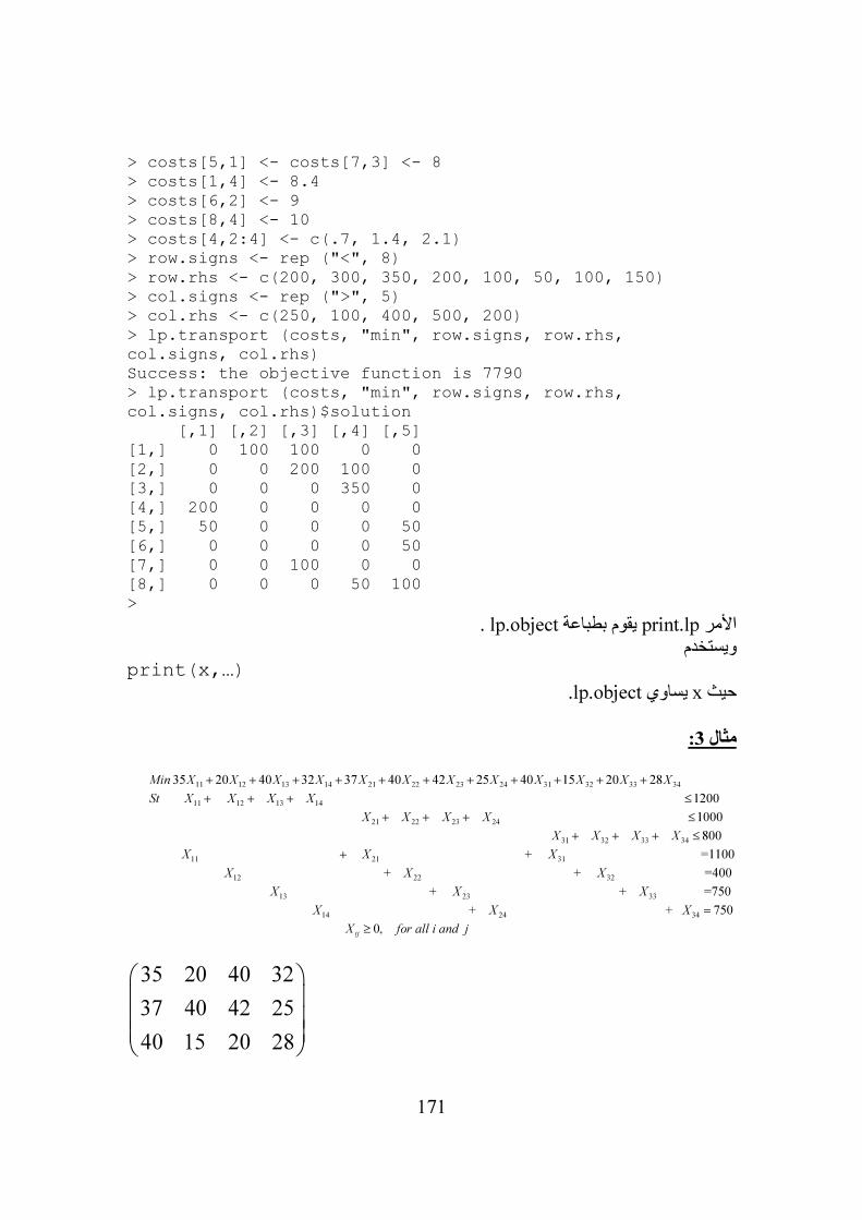
171
> costs[5,1] <- costs[7,3] <- 8 > costs[1,4] <- 8.4 > costs[6,2] <- 9 > costs[8,4] <- 10 > costs[4,2:4] <- c(.7, 1.4, 2.1) > row.signs <- rep ("<", 8) > row.rhs <- c(200, 300, 350, 200, 100, 50, 100, 150) > col.signs <- rep (">", 5) > col.rhs <- c(250, 100, 400, 500, 200) > lp.transport (costs, "min", row.signs, row.rhs, col.signs, col.rhs) Success: the objective function is 7790 > lp.transport (costs, "min", row.signs, row.rhs, col.signs, col.rhs)$solution [,1] [,2] [,3] [,4] [,5] [1,] 0 100 100 0 0 [2,] 0 0 200 100 0 [3,] 0 0 0 350 0 [4,] 200 0 0 0 0 [5,] 50 0 0 0 50 [6,] 0 0 0 0 50 [7,] 0 0 100 0 0 [8,] 0 0 0 50 100 >
. lp.objectيقوم بطباعة print.lpاألمر ويستخدم
print(x,…) .lp.objectيساوي xحيث
:3مثال
11 12 13 14 21 22 23 24 31 32 33 34
11 12 13 14
35 20 40 32 37 40 42 25 40 15 20 28
Min X X X X X X X X X X X X
St X X X X
+ + + + + + + + + + +
+ + +
21 22 23 24
1200
1000
X X X X
≤
+ + + ≤
31 32 33 34
11 21
800
+
X X X X
X X
+ + + ≤
+31
12 22 32
=1100
+ +
X
X X X
13 23 33
=400
+ + =750
X X X
14 24 34 + + 750
X X X =
0,ijX for all i and j≥
35 20 40 32
37 40 42 25
40 15 20 28
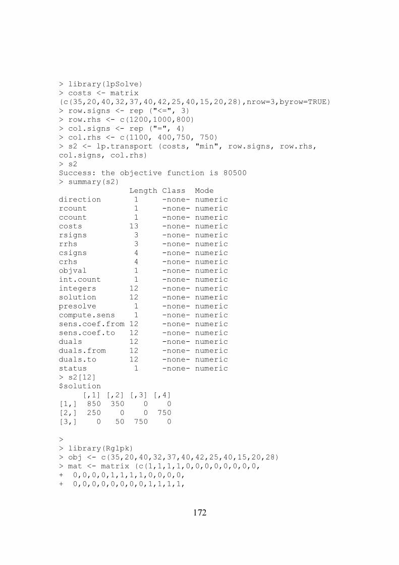
172
> library(lpSolve) > costs <- matrix (c(35,20,40,32,37,40,42,25,40,15,20,28),nrow=3,byrow=TRUE) > row.signs <- rep ("<=", 3) > row.rhs <- c(1200,1000,800) > col.signs <- rep ("=", 4) > col.rhs <- c(1100, 400,750, 750) > s2 <- lp.transport (costs, "min", row.signs, row.rhs, col.signs, col.rhs) > s2 Success: the objective function is 80500 > summary(s2) Length Class Mode direction 1 -none- numeric rcount 1 -none- numeric ccount 1 -none- numeric costs 13 -none- numeric rsigns 3 -none- numeric rrhs 3 -none- numeric csigns 4 -none- numeric crhs 4 -none- numeric objval 1 -none- numeric int.count 1 -none- numeric integers 12 -none- numeric solution 12 -none- numeric presolve 1 -none- numeric compute.sens 1 -none- numeric sens.coef.from 12 -none- numeric sens.coef.to 12 -none- numeric duals 12 -none- numeric duals.from 12 -none- numeric duals.to 12 -none- numeric status 1 -none- numeric > s2[12] $solution [,1] [,2] [,3] [,4] [1,] 850 350 0 0 [2,] 250 0 0 750 [3,] 0 50 750 0 > > library(Rglpk) > obj <- c(35,20,40,32,37,40,42,25,40,15,20,28) > mat <- matrix (c(1,1,1,1,0,0,0,0,0,0,0,0, + 0,0,0,0,1,1,1,1,0,0,0,0, + 0,0,0,0,0,0,0,0,1,1,1,1,
173
+ 1,0,0,0,1,0,0,0,1,0,0,0, + 0,1,0,0,0,1,0,0,0,1,0,0, + 0,0,1,0,0,0,1,0,0,0,1,0, + 0,0,0,1,0,0,0,1,0,0,0,1),nrow=7,byrow=TRUE) > dir <- c(rep("<=",3),rep("==",4)) > rhs <- c(1200,1000,800,1100,400,750,750) > s3 <- Rglpk_solve_LP(obj, mat, dir, rhs, types = "I") > s3 $optimum [1] 80500 $solution [1] 850 350 0 0 250 0 0 750 0 50 750 0 $status [1] 0 > > library(lpSolve) > costs <- matrix (c(35,20,40,32,37,40,42,25,40,15,20,28),nrow=3,byrow=TRUE) > row.signs <- rep ("<=", 3) > row.rhs <- c(1200,1000,800) > col.signs <- rep ("=", 4) > col.rhs <- c(1100, 400,750, 750) > s2 <- lp.transport (costs, "min", row.signs, row.rhs, col.signs, col.rhs) > print(s2) Success: the objective function is 80500 >
Transportation Problemمثال آخرلمشكلة نقل
لشركة مصنعين إلنتاج معين والذي يتم توزيعه عن طريق ثالثة مراكز توزيع. سعر إنتاج الوحدة متساوي في جميع المصانع ولكن تكلفة النقل من المصانع إلى مراكز التوزيع تختلف حسب البيانات
في الجدول التالي: Distribution
Center 1 Distribution Center 2
Distribution Center 3
Plant A 4 6 4 Plant B 6 5 2
وحدة وكل مركز 60عملية النقل تتم مرة في األسبوع. خالل األسبوع كل مصنع ينتج على األكثر
وحدة للتوزيع. 40توزيع يحتاج
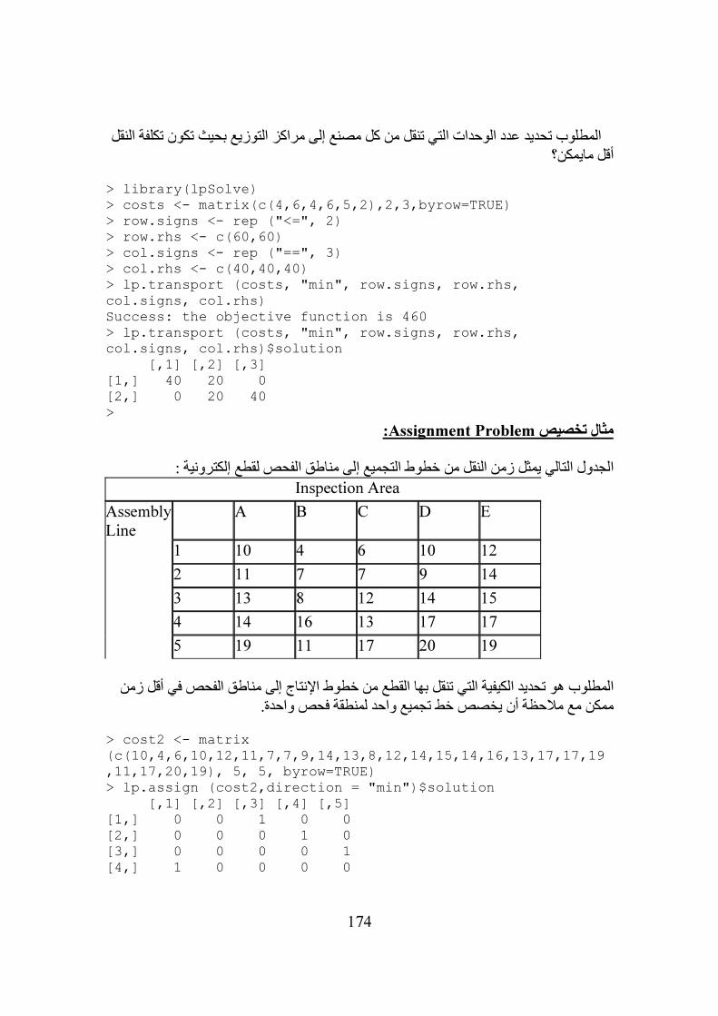
174
توزيع بحيث تكون تكلفة النقل المطلوب تحديد عدد الوحدات التي تنقل من كل مصنع إلى مراكز ال أقل مايمكن؟
> library(lpSolve) > costs <- matrix(c(4,6,4,6,5,2),2,3,byrow=TRUE) > row.signs <- rep ("<=", 2) > row.rhs <- c(60,60) > col.signs <- rep ("==", 3) > col.rhs <- c(40,40,40) > lp.transport (costs, "min", row.signs, row.rhs, col.signs, col.rhs) Success: the objective function is 460 > lp.transport (costs, "min", row.signs, row.rhs, col.signs, col.rhs)$solution [,1] [,2] [,3] [1,] 40 20 0 [2,] 0 20 40 >
:Assignment Problemمثال تخصيص
:مثل زمن النقل من خطوط التجميع إلى مناطق الفحص لقطع إلكترونيةالجدول التالي ي Inspection Area
AssemblyLine
A B C D E
1 10 4 6 10 12
2 11 7 7 9 14
3 13 8 12 14 15
4 14 16 13 17 17
5 19 11 17 20 19
ديد الكيفية التي تنقل بها القطع من خطوط اإلنتاج إلى مناطق الفحص في أقل زمن المطلوب هو تح ممكن مع مالحظة أن يخصص خط تجميع واحد لمنطقة فحص واحدة.
> cost2 <- matrix (c(10,4,6,10,12,11,7,7,9,14,13,8,12,14,15,14,16,13,17,17,19,11,17,20,19), 5, 5, byrow=TRUE) > lp.assign (cost2,direction = "min")$solution [,1] [,2] [,3] [,4] [,5] [1,] 0 0 1 0 0 [2,] 0 0 0 1 0 [3,] 0 0 0 0 1 [4,] 1 0 0 0 0

175
[5,] 0 1 0 0 0 >
176
مشكلة الجراب:
)من المتغيرات الثنائية من األشياء. المتجة nلدينا ), 1,...,j
x j n= :والذي له الخاصية التالية
1
0j
if object j is selectedx
otherwise
=
)فإذا كانت ), 1,...,j
p j n= (شيئ) مقياس أهمية العنصرj و( ), 1,...,j
w j n= حجم (او
فالمشكلة هي في إختيار من بين كل حجم أوسعة الحقيبة الظهرية cو jوزن) العنصر (شيئ) والتي تحقق القيود xالمتجهات الثنائية
1
n
j j
j
w x c
=
≤∑
دالة الهدف maximizesتلك التي تعظم
1
n
j j
j
p x
=
∑
أي
maximize 1
n
j j
j
p x
=
∑
subject to 1
n
j j
j
w x c
=
≤∑
0 1, 1,...,j
x or j n= =
مثال:
( )
( )
8
15,100,90,60,40,15,10,1
2,20,20,30,40,30,60,10
102
j
j
n
p
w
c
=
=
=
=
> library(lpSolve) > f.obj <- c(15,100,90,60,40,15,10,1) > f.con <- matrix(c(2,20,20,30,40,30,60,10),1,8,byrow=TRUE) > f.dir <- c("<=") > f.rhs <- c(102) > s1 <- lp ("max", f.obj, f.con, f.dir, f.rhs,binary.vec=1:8) > lp ("max", f.obj, f.con, f.dir, f.rhs,binary.vec=1:8)$solution
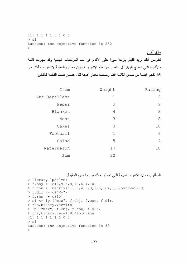
177
[1] 1 1 1 1 0 1 0 0 > s1 Success: the objective function is 280 >
مثال آخر:
لنفرض أنك تريد القيام بنزهة سيرا على األقدام في أحد المرتفعات الجبلية وقد جهزت قائمة
ج إليها. كل عنصر من هذه اإلشياء له وزن معين والحقيبة التستوعب أكثر من باألشياء التي تحتا
كجم. ايضا من ضمن القائمة انت وضعت معيار أهمية لكل عنصر فبدت القائمة كالتالي: 15
Item Weight Rating
Ant Repellent 1 2
Pepsi 3 9
Blanket 4 3
Meat 3 8
Cakes 3 10
Football 1 6
Salad 5 4
Watermelon 10 10
Sum 30
المطلوب تحديد األشياء المهمة التي تحملها معك مراعيا حجم الحقيبة.
> library(lpSolve) > f.obj <- c(2,9,3,8,10,6,4,10) > f.con <- matrix(c(1,3,4,3,3,1,5,10),1,8,byrow=TRUE) > f.dir <- c("<=") > f.rhs <- c(15) > s1 <- lp ("max", f.obj, f.con, f.dir, f.rhs,binary.vec=1:8) > lp ("max", f.obj, f.con, f.dir, f.rhs,binary.vec=1:8)$solution [1] 1 1 1 1 1 1 0 0 > s1 Success: the objective function is 38 >
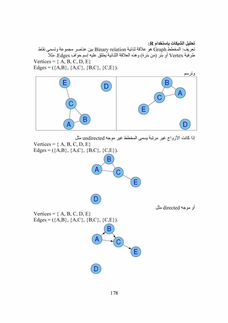
178
:Rتحليل الشبكات بإستخدام بين عناصر مجموعة وتسمى نقاط Binary relationهو عالقة ثنائية Graphتعريف: المخطط
. مثال Edgesأو بئر (من بئرة) وهذه العالقة الثنائية يطلق عليه إسم حواف Vertexطرفية
Vertices = { A, B, C, D, E} Edges = ({A,B}, {A,C}, {B,C}, {C,E}).
وترسم
مثل undirectedإذا كانت األزواج غير مرتبة يسمى المخطط غير موجه Vertices = { A, B, C, D, E} Edges = ({A,B}, {A,C}, {B,C}, {C,E}).
مثل directedأو موجه
Vertices = { A, B, C, D, E} Edges = ({A,B}, {A,C}, {B,C}, {C,E}).
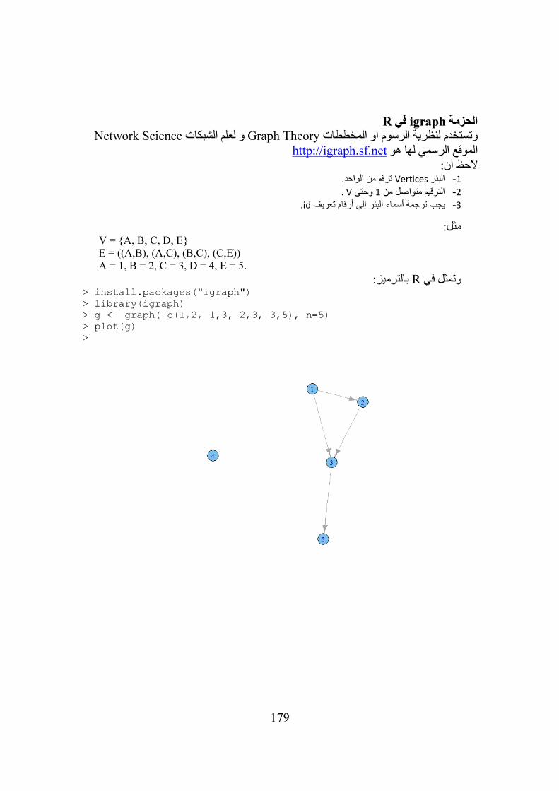
179
Rفي igraphالحزمة
Network Scienceو لعلم الشبكات Graph Theoryوتستخدم لنظرية الرسوم او المخططات
http://igraph.sf.netالموقع الرسمي لها هو الحظ ان:
ترقم من الواحد. Verticesالبئر -1
V .وحتى 1الترقيم متواصل من -2
.idيجب ترجمة أسماء البئر إلى أرقام تعريف -3
مثل:V = {A, B, C, D, E}
E = ((A,B), (A,C), (B,C), (C,E))
A = 1, B = 2, C = 3, D = 4, E = 5.
:بالترميز Rوتمثل في > install.packages("igraph")
> library(igraph)
> g <- graph( c(1,2, 1,3, 2,3, 3,5), n=5)
> plot(g)
>
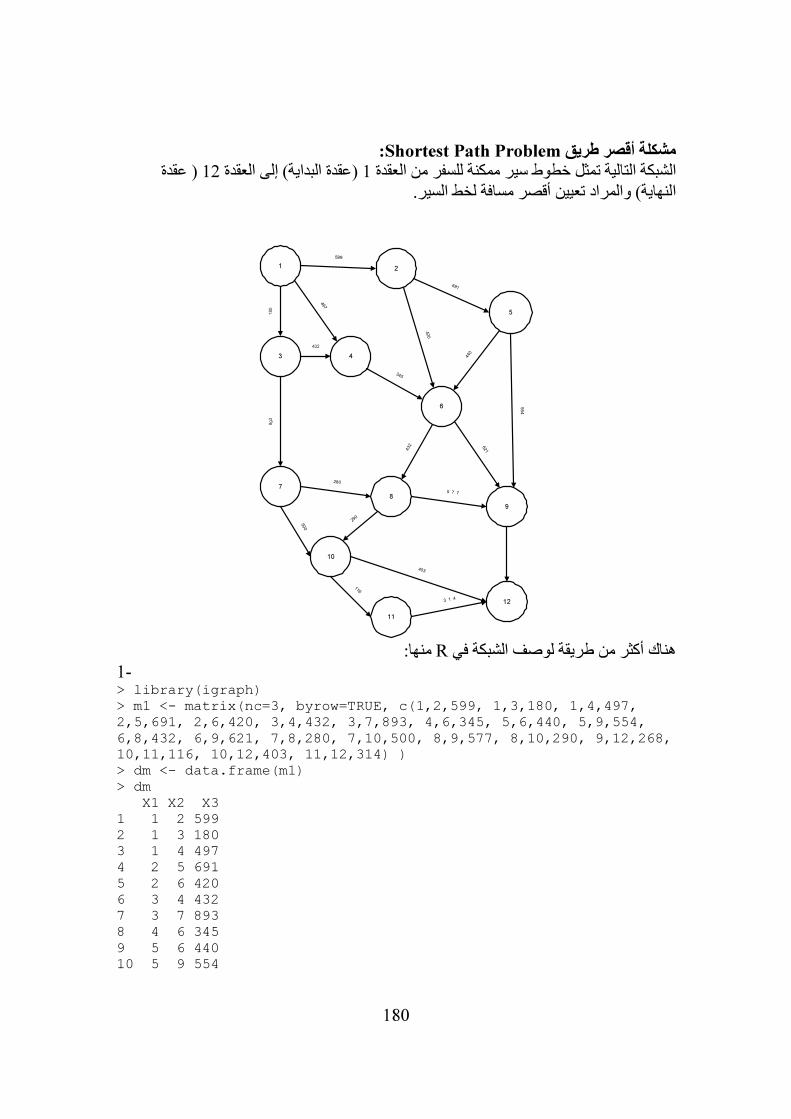
180
:Shortest Path Problemمشكلة أقصر طريق ( عقدة 12داية) إلى العقدة (عقدة الب 1الشبكة التالية تمثل خطوط سير ممكنة للسفر من العقدة
النهاية) والمراد تعيين أقصر مسافة لخط السير.
12
3 4
5
6
7
8
9
10
11
12
599
180
497
432
345
420
440
691
893
280
500
290
5 7 7
116
403
3 1 4
432 6
21
554
منها: Rهناك أكثر من طريقة لوصف الشبكة في
1- > library(igraph)
> m1 <- matrix(nc=3, byrow=TRUE, c(1,2,599, 1,3,180, 1,4,497,
2,5,691, 2,6,420, 3,4,432, 3,7,893, 4,6,345, 5,6,440, 5,9,554,
6,8,432, 6,9,621, 7,8,280, 7,10,500, 8,9,577, 8,10,290, 9,12,268,
10,11,116, 10,12,403, 11,12,314) )
> dm <- data.frame(m1)
> dm
X1 X2 X3
1 1 2 599
2 1 3 180
3 1 4 497
4 2 5 691
5 2 6 420
6 3 4 432
7 3 7 893
8 4 6 345
9 5 6 440
10 5 9 554
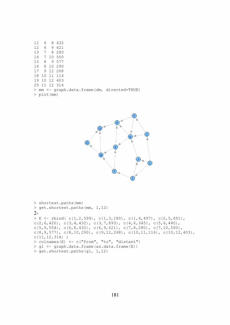
181
11 6 8 432
12 6 9 621
13 7 8 280
14 7 10 500
15 8 9 577
16 8 10 290
17 9 12 268
18 10 11 116
19 10 12 403
20 11 12 314
> mm <- graph.data.frame(dm, directed=TRUE)
> plot(mm)
> shortest.paths(mm)
> get.shortest.paths(mm, 1,12)
2- > E <- rbind( c(1,2,599), c(1,3,180), c(1,4,497), c(2,5,691),
c(2,6,420), c(3,4,432), c(3,7,893), c(4,6,345), c(5,6,440),
c(5,9,554), c(6,8,432), c(6,9,621), c(7,8,280), c(7,10,500),
c(8,9,577), c(8,10,290), c(9,12,268), c(10,11,116), c(10,12,403),
c(11,12,314) )
> colnames(E) <- c("from", "to", "distant")
> g1 <- graph.data.frame(as.data.frame(E))
> get.shortest.paths(g1, 1,12)
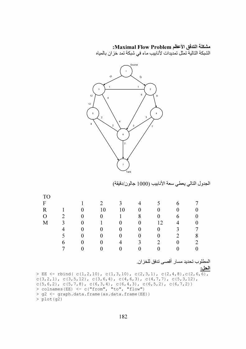
182
:Maximal Flow Problemمشكلة التدفق األعظم الشبكة التالية تمثل تمديدات ألنابيب ماء في شبكة تمد خزان بالمياه
1
23
45
6
7
1010
1 1
4
4
12
2
2
68
7
3
3
2
8
12
Source
Tank
جالون/دقيقة) 1000الجدول التالي يعطي سعة األنابيب (
TO 7 6 5 4 3 2 1 F
R O M
0 0 0 0 10 10 0 1 0 6 0 8 1 0 0 2 0 4 12 0 0 1 0 3 7 3 0 0 0 0 0 4 8 2 0 0 0 0 0 5 2 0 2 3 4 0 0 6 0 0 0 0 0 0 0 7
المطلوب تحديد مسار أقصى تدفق للخزان.
الحل:> EE <- rbind( c(1,2,10), c(1,3,10), c(2,3,1), c(2,4,8),c(2,6,6),
c(3,2,1), c(3,5,12), c(3,6,4), c(4,6,3), c(4,7,7), c(5,3,12),
c(5,6,2), c(5,7,8), c(6,3,4), c(6,4,3), c(6,5,2), c(6,7,2))
> colnames(EE) <- c("from", "to", "flow")
> g2 <- graph.data.frame(as.data.frame(EE))
> plot(g2)
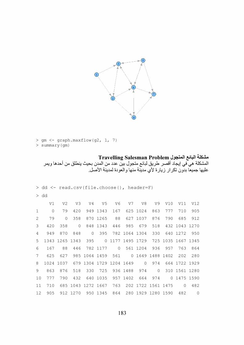
183
> gm <- graph.maxflow(g2, 1, 7)
> summary(gm)
Travelling Salesman Problemمشكلة البائع المتجول
بين عدد من المدن بحيث ينطلق من أحدها ويمر هي في إيجاد أقصر طريق لبائع متجول المشكلة عليها جميعا بدون تكرار زيارة ألي مدينة منها والعودة لمدينة األصل.
> dd <- read.csv(file.choose(), header=F)
> dd
V1 V2 V3 V4 V5 V6 V7 V8 V9 V10 V11 V12
1 0 79 420 949 1343 167 625 1024 863 777 710 905
2 79 0 358 870 1265 88 627 1037 876 790 685 912
3 420 358 0 848 1343 446 985 679 518 432 1043 1270
4 949 870 848 0 395 782 1064 1304 330 640 1272 950
5 1343 1265 1343 395 0 1177 1495 1729 725 1035 1667 1345
6 167 88 446 782 1177 0 561 1204 936 957 763 864
7 625 627 985 1064 1459 561 0 1649 1488 1402 202 280
8 1024 1037 679 1304 1729 1204 1649 0 974 664 1722 1929
9 863 876 518 330 725 936 1488 974 0 310 1561 1280
10 777 790 432 640 1035 957 1402 664 974 0 1475 1590
11 710 685 1043 1272 1667 763 202 1722 1561 1475 0 482
12 905 912 1270 950 1345 864 280 1929 1280 1590 482 0
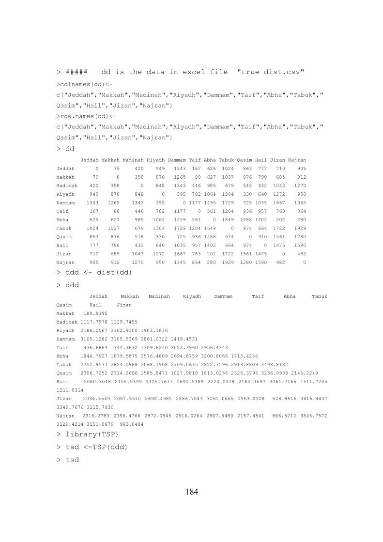
184
> ##### dd is the data in excel file "true dist.csv"
>colnames(dd)<-
c("Jeddah","Makkah","Madinah","Riyadh","Dammam","Taif","Abha","Tabuk","
Qasim","Hail","Jizan","Najran")
>row.names(dd)<-
c("Jeddah","Makkah","Madinah","Riyadh","Dammam","Taif","Abha","Tabuk","
Qasim","Hail","Jizan","Najran")
> dd
Jeddah Makkah Madinah Riyadh Dammam Taif Abha Tabuk Qasim Hail Jizan Najran
Jeddah 0 79 420 949 1343 167 625 1024 863 777 710 905
Makkah 79 0 358 870 1265 88 627 1037 876 790 685 912
Madinah 420 358 0 848 1343 446 985 679 518 432 1043 1270
Riyadh 949 870 848 0 395 782 1064 1304 330 640 1272 950
Dammam 1343 1265 1343 395 0 1177 1495 1729 725 1035 1667 1345
Taif 167 88 446 782 1177 0 561 1204 936 957 763 864
Abha 625 627 985 1064 1459 561 0 1649 1488 1402 202 280
Tabuk 1024 1037 679 1304 1729 1204 1649 0 974 664 1722 1929
Qasim 863 876 518 330 725 936 1488 974 0 310 1561 1280
Hail 777 790 432 640 1035 957 1402 664 974 0 1475 1590
Jizan 710 685 1043 1272 1667 763 202 1722 1561 1475 0 482
Najran 905 912 1270 950 1345 864 280 1929 1280 1590 482 0
> ddd <- dist(dd)
> ddd
Jeddah Makkah Madinah Riyadh Dammam Taif Abha Tabuk
Qasim Hail Jizan
Makkah 189.9395
Madinah 1117.7978 1129.7455
Riyadh 2186.0567 2162.9200 1903.1836
Dammam 3105.1282 3105.9369 2861.0322 1419.4531
Taif 436.6864 344.3632 1309.8240 2053.3960 2956.4343
Abha 1844.7927 1879.5875 2576.4809 2694.8759 3200.8066 1713.4255
Tabuk 2752.9571 2824.0988 2068.1908 2709.0635 2822.7596 2913.8809 3498.8182
Qasim 2306.7252 2314.2606 1585.8471 1027.9810 1813.0256 2326.3796 3236.9938 2145.2249
Hail 2080.3048 2105.9399 1325.7617 1690.5189 2220.0318 2184.3697 3061.7165 1511.7205
1211.0314
Jizan 2036.5549 2087.5510 2692.4985 2886.7043 3261.0665 1963.2328 528.8516 3416.8437
3349.7676 3115.7930
Najran 2316.2783 2356.4766 2872.0945 2516.0264 2807.5480 2157.4541 866.5212 3545.7572
3129.4214 3151.0879 982.0484
> library(TSP)
> tsd <-TSP(ddd)
> tsd
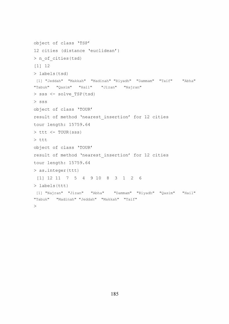
185
object of class ‘TSP’
12 cities (distance ‘euclidean’)
> n_of_cities(tsd)
[1] 12
> labels(tsd)
[1] "Jeddah" "Makkah" "Madinah" "Riyadh" "Dammam" "Taif" "Abha"
"Tabuk" "Qasim" "Hail" "Jizan" "Najran"
> sss <- solve_TSP(tsd)
> sss
object of class ‘TOUR’
result of method ‘nearest_insertion’ for 12 cities
tour length: 15759.64
> ttt <- TOUR(sss)
> ttt
object of class ‘TOUR’
result of method ‘nearest_insertion’ for 12 cities
tour length: 15759.64
> as.integer(ttt)
[1] 12 11 7 5 4 9 10 8 3 1 2 6
> labels(ttt)
[1] "Najran" "Jizan" "Abha" "Dammam" "Riyadh" "Qasim" "Hail"
"Tabuk" "Madinah" "Jeddah" "Makkah" "Taif"
>
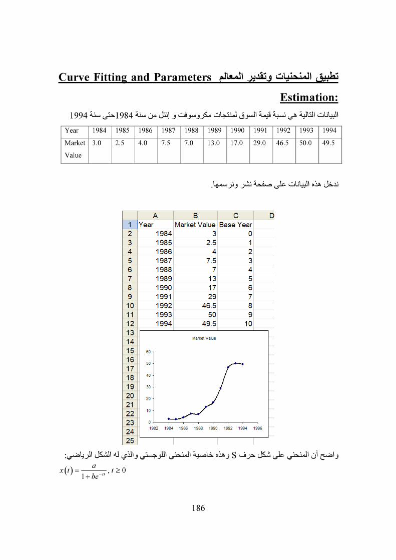
186
Curve Fitting and Parametersتطبيق المنحنيات وتقدير المعالم
Estimation:
1994حتى سنة 1984البيانات التالية هي نسبة قيمة السوق لمنتجات مكروسوفت و إنتل من سنة
1994 1993 1992 1991 1990 1989 1988 1987 1986 1985 1984 Year
49.5 50.0 46.5 29.0 17.0 13.0 7.0 7.5 4.0 2.5 3.0 Market
Value
ندخل هذه البيانات على صفحة نشر ونرسمها.
وهذه خاصية المنحنى اللوجستي والذي له الشكل الرياضي: Sواضح أن المنحني على شكل حرف
( ) , 01
ct
ax t t
be−
= ≥
+
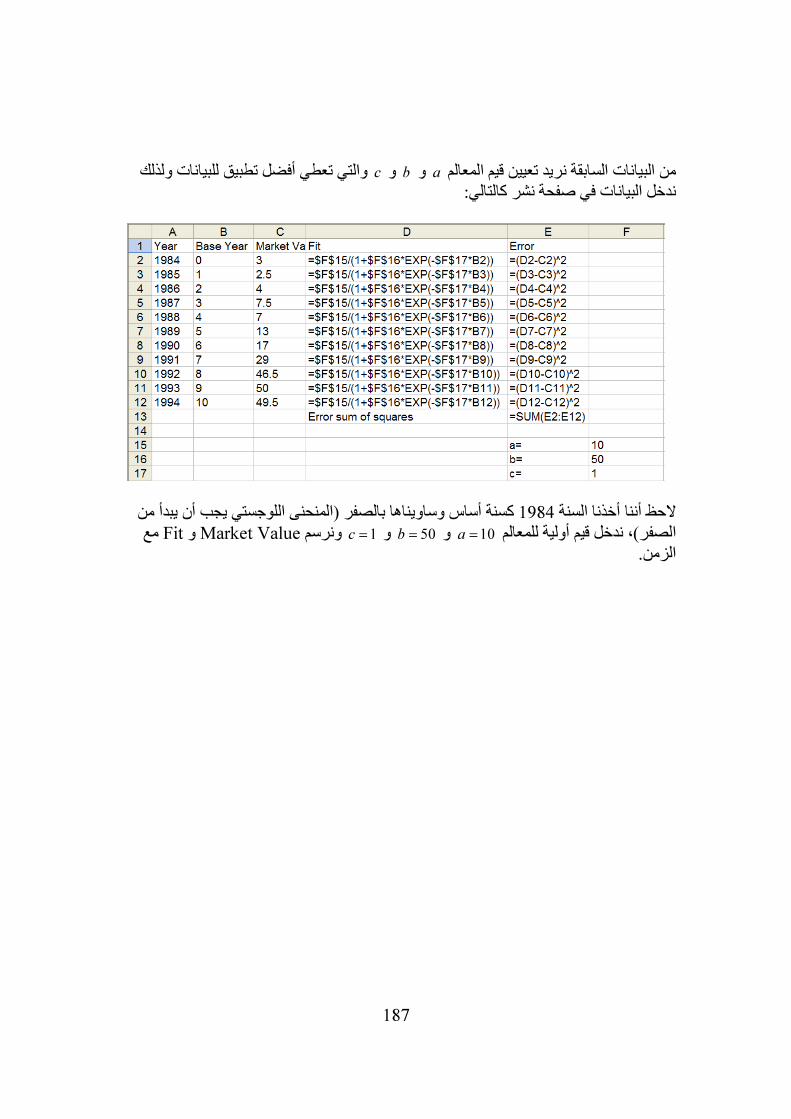
187
والتي تعطي أفضل تطبيق للبيانات ولذلك cو bو aقيم المعالم من البيانات السابقة نريد تعيين
ندخل البيانات في صفحة نشر كالتالي:
يبدأ من كسنة أساس وساويناها بالصفر (المنحنى اللوجستي يجب أن 1984الحظ أننا أخذنا السنة 10aالصفر)، ندخل قيم أولية للمعالم 50bو = 1cو = مع Fitو Market Valueونرسم =
الزمن.
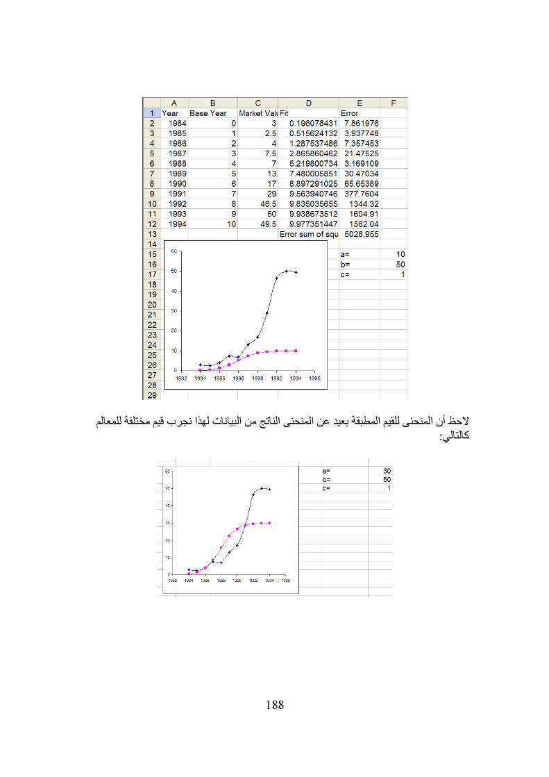
188
معالم الحظ أن المنحنى للقيم المطبقة بعيد عن المنحنى الناتج من البيانات لهذا نجرب قيم مختلفة لل كالتالي:
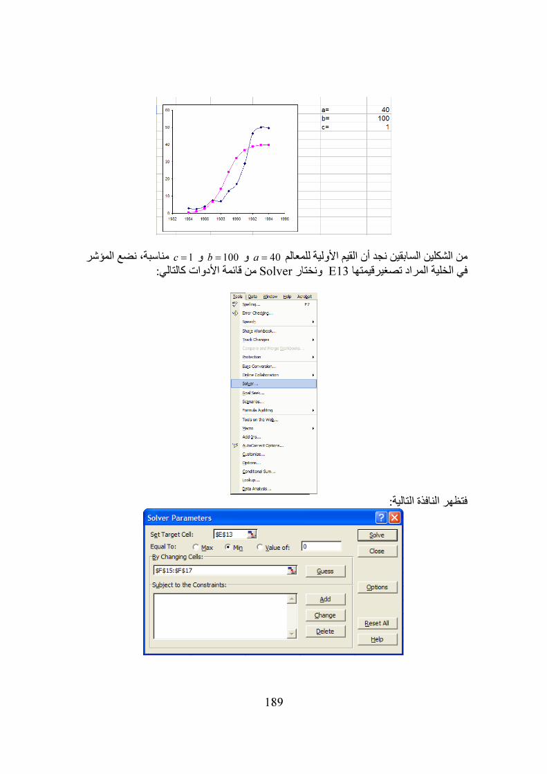
189
40aمن الشكلين السابقين نجد أن القيم األولية للمعالم 100bو = 1cو = مناسبة، نضع المؤشر = من قائمة األدوات كالتالي: Solverونختار E13في الخلية المراد تصغيرقيمتها
فتظهر النافذة التالية:
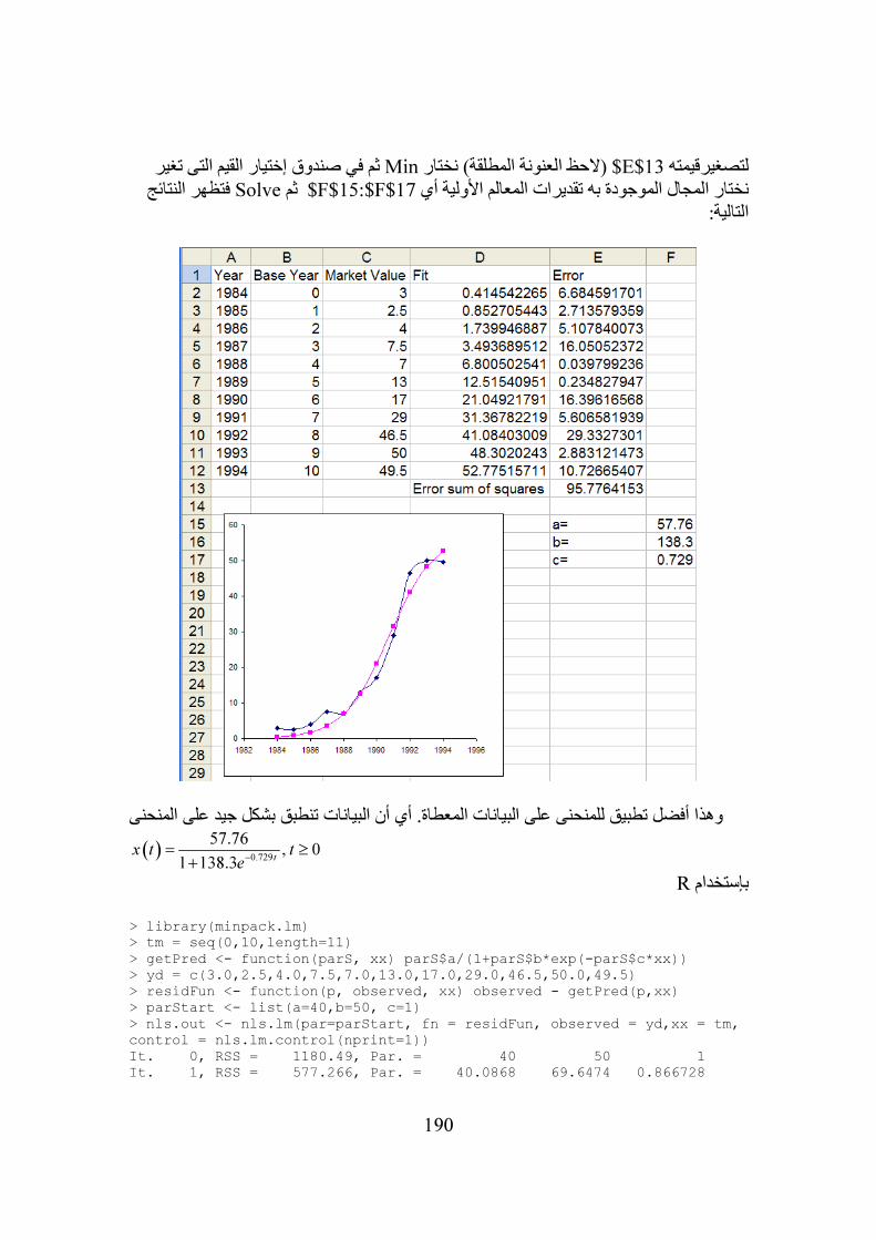
190
ثم في صندوق إختيار القيم التى تغير Min(الحظ العنونة المطلقة) نختار E$13$لتصغيرقيمته فتظهر النتائج Solveثم F$15:$F$17$نختار المجال الموجودة به تقديرات المعالم األولية أي
التالية:
ة. أي أن البيانات تنطبق بشكل جيد على المنحنىوهذا أفضل تطبيق للمنحنى على البيانات المعطا
( )0.729
57.76, 0
1 138.3t
x t t
e−
= ≥
+
Rبإستخدام > library(minpack.lm)
> tm = seq(0,10,length=11)
> getPred <- function(parS, xx) parS$a/(1+parS$b*exp(-parS$c*xx))
> yd = c(3.0,2.5,4.0,7.5,7.0,13.0,17.0,29.0,46.5,50.0,49.5)
> residFun <- function(p, observed, xx) observed - getPred(p,xx)
> parStart <- list(a=40,b=50, c=1)
> nls.out <- nls.lm(par=parStart, fn = residFun, observed = yd,xx = tm,
control = nls.lm.control(nprint=1))
It. 0, RSS = 1180.49, Par. = 40 50 1
It. 1, RSS = 577.266, Par. = 40.0868 69.6474 0.866728
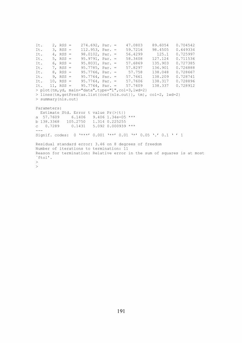
191
It. 2, RSS = 274.692, Par. = 47.0803 89.6054 0.704542
It. 3, RSS = 112.953, Par. = 59.7216 98.4505 0.649334
It. 4, RSS = 98.0102, Par. = 56.4299 125.1 0.725997
It. 5, RSS = 95.9791, Par. = 58.3408 127.124 0.711536
It. 6, RSS = 95.8031, Par. = 57.6869 135.903 0.727385
It. 7, RSS = 95.7785, Par. = 57.8297 136.901 0.726888
It. 8, RSS = 95.7766, Par. = 57.758 138.048 0.728667
It. 9, RSS = 95.7764, Par. = 57.7661 138.209 0.728741
It. 10, RSS = 95.7764, Par. = 57.7606 138.317 0.728896
It. 11, RSS = 95.7764, Par. = 57.7609 138.337 0.728912
> plot(tm,yd, main="data",type="l",col=3,lwd=2)
> lines(tm,getPred(as.list(coef(nls.out)), tm), col=2, lwd=2)
> summary(nls.out)
Parameters:
Estimate Std. Error t value Pr(>|t|)
a 57.7609 6.1406 9.406 1.34e-05 ***
b 138.3368 105.2750 1.314 0.225255
c 0.7289 0.1431 5.092 0.000939 ***
---
Signif. codes: 0 ‘***’ 0.001 ‘**’ 0.01 ‘*’ 0.05 ‘.’ 0.1 ‘ ’ 1
Residual standard error: 3.46 on 8 degrees of freedom
Number of iterations to termination: 11
Reason for termination: Relative error in the sum of squares is at most
`ftol'.
>
>
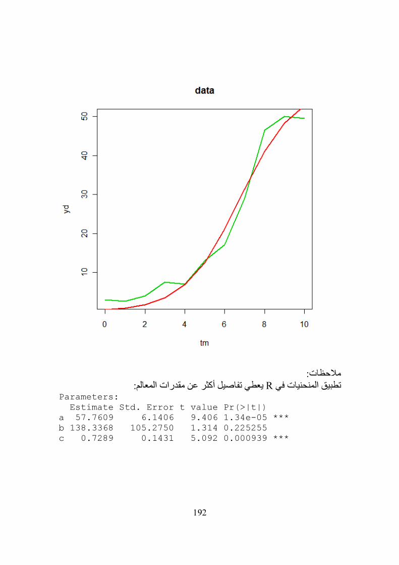
192
مالحظات: يعطي تفاصيل أكثر عن مقدرات المعالم: Rتطبيق المنحنيات في
Parameters: Estimate Std. Error t value Pr(>|t|) a 57.7609 6.1406 9.406 1.34e-05 *** b 138.3368 105.2750 1.314 0.225255 c 0.7289 0.1431 5.092 0.000939 ***

193
مثال آخر لتطبيق المنحنيات
Jظاهرة المنحنى
Stateوالذي فيه يتفاعل متغيرين حالة Jكثير من األنظمة الطبيعية تبدي ظاهرة منحنى
Variables لى بحيث تتناقص قيمة المتغير التابع مع زيادة المتغير المستقل حتى يصل إ
نقطة حرجة ثم يعود
في الزيادة ويتخطى
نقطة تفاعلة السابقة.
هو تأثير تخفيض سعر الصرف لعملة على Jومن األمثلة الشهيرة على ظاهرة منحنى
ميزان التعامالت مقاس بالعملة المحلية والذي سوف يزداد سوء في فترة صدمة القرار
صادرات رخيصة وواردات ثم يعود للتحسن. تخفيض معدل الصرف سوف يؤدي ل
غالية مما يجعل التوازن الحالى أكثر سوء ولكن بعد فترة فإن حجم الصادرات سوف
يبدأ في اإلرتفاع بسبب رخص أسعارها بالنسبة للمشتري األجنبي كما أن المستهلك
المحلي سوف يقلل من شرائه للبضائع المستوردة التي أصبحت غالية الثمن. وبالتدريج
المدفوعات أو التعامالت أو التجاري سوف يتحسن.فإن ميزان
تتناقص Venture Fundمثال قد يعني أن قيمة اإلعتماد المالي المجازف Jالمنحنى
يصبح سالبا في Internal Rate of Return (IRR) دائما و المعدل الضمني للربح
تعني إنتكاس Jحنى السنوات القليلة القادمة قبل أن يبدأ كليهما في الصعود. ففرضية من
قصير األمد يتبعه تحسن طويل األمد.
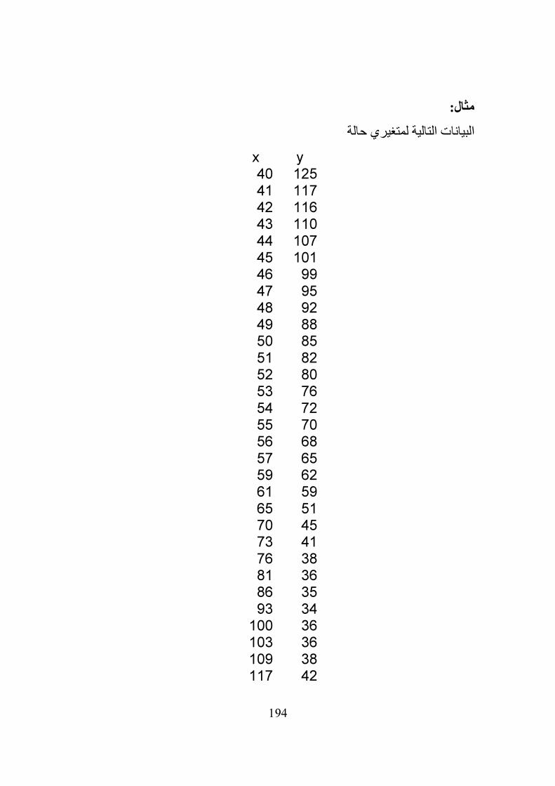
194
مثال:
البيانات التالية لمتغيري حالة
x y 40 125 41 117 42 116 43 110 44 107 45 101 46 99 47 95 48 92 49 88 50 85 51 82 52 80 53 76 54 72 55 70 56 68 57 65 59 62 61 59 65 51 70 45 73 41 76 38 81 36 86 35 93 34
100 36 103 36 109 38 117 42
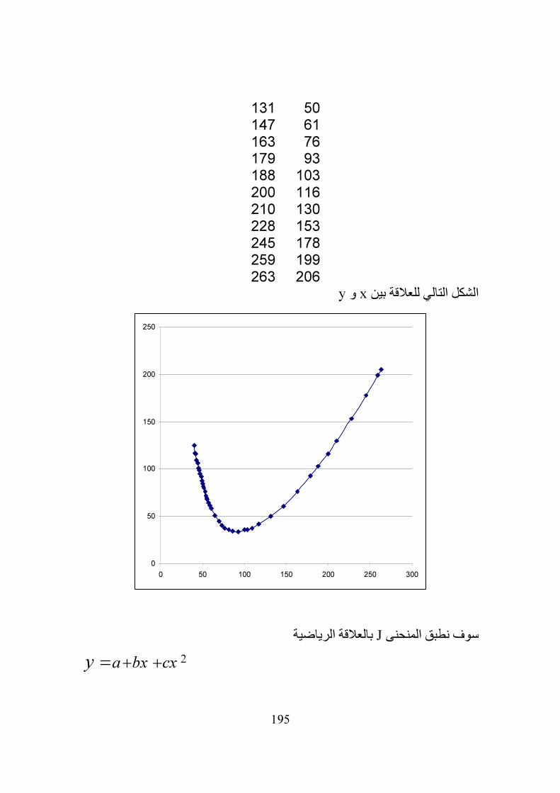
195
131 50 147 61 163 76 179 93 188 103 200 116 210 130 228 153 245 178 259 199 263 206
yو xالشكل التالي للعالقة بين
0
50
100
150
200
250
0 50 100 150 200 250 300
بالعالقة الرياضية Jسوف نطبق المنحنى
2a bx cxy + +=
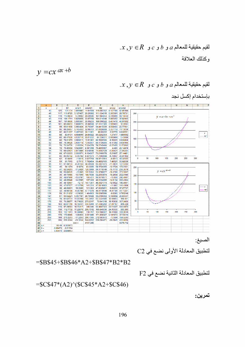
196
x,و cو bو aلقيم حقيقية للمعالم y R∈.
وكذلك العالقة
ax by cx +=
x,و cو bو aلقيم حقيقية للمعالم y R∈.
بإستخدام إكسل نجد
الصيغ:
C2لتطبيق المعادلة األولى نضع في
=$B$45+$B$46*A2+$B$47*B2*B2
F2لتطبيق المعادلة الثانية نضع في
=$C$47*(A2)^($C$45*A2+$C$46)
تمرين:
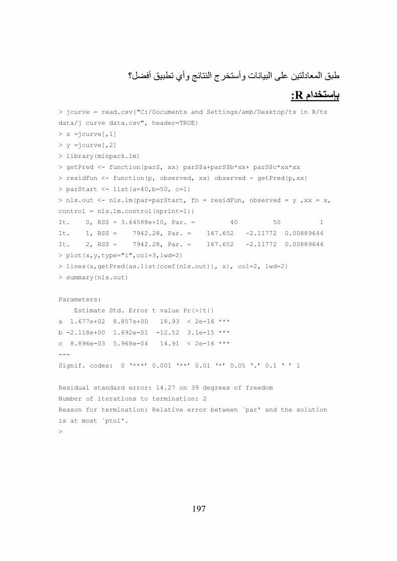
197
طبق المعادلتين على البيانات وأستخرج النتائج وأي تطبيق أفضل؟
:Rبإستخدام
> jcurve = read.csv("C:/Documents and Settings/amb/Desktop/ts in R/ts
data/j curve data.csv", header=TRUE)
> x =jcurve[,1]
> y =jcurve[,2]
> library(minpack.lm)
> getPred <- function(parS, xx) parS$a+parS$b*xx+ parS$c*xx*xx
> residFun <- function(p, observed, xx) observed - getPred(p,xx)
> parStart <- list(a=40,b=50, c=1)
> nls.out <- nls.lm(par=parStart, fn = residFun, observed = y ,xx = x,
control = nls.lm.control(nprint=1))
It. 0, RSS = 3.64588e+10, Par. = 40 50 1
It. 1, RSS = 7942.28, Par. = 167.652 -2.11772 0.00889644
It. 2, RSS = 7942.28, Par. = 167.652 -2.11772 0.00889644
> plot(x,y,type="l",col=3,lwd=2)
> lines(x,getPred(as.list(coef(nls.out)), x), col=2, lwd=2)
> summary(nls.out)
Parameters:
Estimate Std. Error t value Pr(>|t|)
a 1.677e+02 8.857e+00 18.93 < 2e-16 ***
b -2.118e+00 1.692e-01 -12.52 3.1e-15 ***
c 8.896e-03 5.968e-04 14.91 < 2e-16 ***
---
Signif. codes: 0 ‘***’ 0.001 ‘**’ 0.01 ‘*’ 0.05 ‘.’ 0.1 ‘ ’ 1
Residual standard error: 14.27 on 39 degrees of freedom
Number of iterations to termination: 2
Reason for termination: Relative error between `par' and the solution
is at most `ptol'.
>
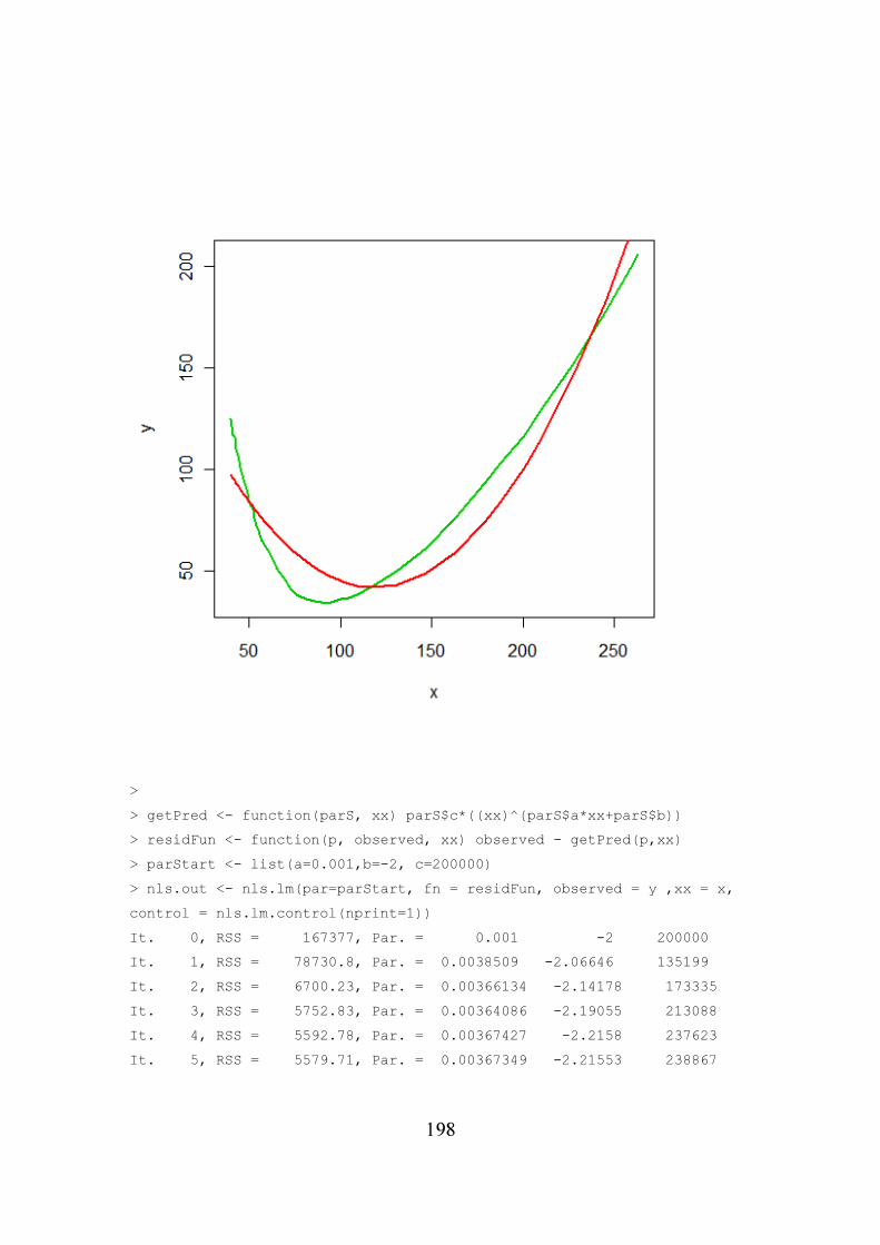
198
>
> getPred <- function(parS, xx) parS$c*((xx)^(parS$a*xx+parS$b))
> residFun <- function(p, observed, xx) observed - getPred(p,xx)
> parStart <- list(a=0.001,b=-2, c=200000)
> nls.out <- nls.lm(par=parStart, fn = residFun, observed = y ,xx = x,
control = nls.lm.control(nprint=1))
It. 0, RSS = 167377, Par. = 0.001 -2 200000
It. 1, RSS = 78730.8, Par. = 0.0038509 -2.06646 135199
It. 2, RSS = 6700.23, Par. = 0.00366134 -2.14178 173335
It. 3, RSS = 5752.83, Par. = 0.00364086 -2.19055 213088
It. 4, RSS = 5592.78, Par. = 0.00367427 -2.2158 237623
It. 5, RSS = 5579.71, Par. = 0.00367349 -2.21553 238867
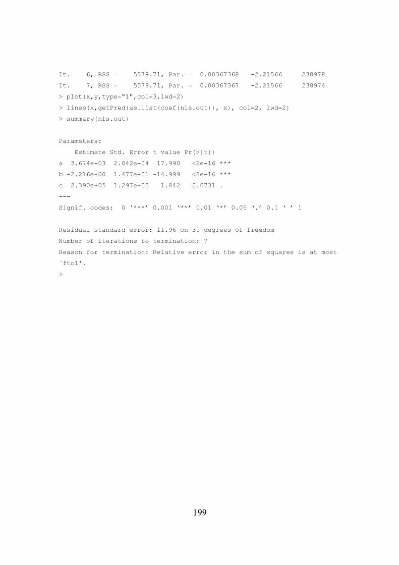
199
It. 6, RSS = 5579.71, Par. = 0.00367368 -2.21566 238978
It. 7, RSS = 5579.71, Par. = 0.00367367 -2.21566 238974
> plot(x,y,type="l",col=3,lwd=2)
> lines(x,getPred(as.list(coef(nls.out)), x), col=2, lwd=2)
> summary(nls.out)
Parameters:
Estimate Std. Error t value Pr(>|t|)
a 3.674e-03 2.042e-04 17.990 <2e-16 ***
b -2.216e+00 1.477e-01 -14.999 <2e-16 ***
c 2.390e+05 1.297e+05 1.842 0.0731 .
---
Signif. codes: 0 ‘***’ 0.001 ‘**’ 0.01 ‘*’ 0.05 ‘.’ 0.1 ‘ ’ 1
Residual standard error: 11.96 on 39 degrees of freedom
Number of iterations to termination: 7
Reason for termination: Relative error in the sum of squares is at most
`ftol'.
>
200
201
ملحق:
Rمقدمة للغة النمذجة الرياضية
البيانات وإدارة الدورة وإحصائآت بسيطة:
أفكار أساسية:
:Objectsأشياء
. جميع األشياء تمتلك الخواص التالية والتي نطلق عليها Objectsعلى أشياء Rتعمل : intrinsic attributesالصفات الجوهرية
والصيغ الممكنة هنا هي: عددي - الشيئ : ويبين نوعmodeنمط أو صيغة •numeric أو مركب complex أو منطقي logical أو نص character أو
.listقائمة

202
: عدد المكونات والتي تصنع الشيئ.lengthطول •وببساطة الشيئ هو طريقة مناسبة لتخزين المعلومات. ففي النمذجة الرياضية نحتاج
ة. وهذا يتم عن طريق إستخدام متجه عددي. الحظ انه لتخزين مشاهدات لمتغير ذو أهمي. المتجهات 1فالعدد الفردي هو متجه عددي له طول Rفي Scalarاليوجد قيم مفردة
حيث جميع مكوناتها لها نفس النمط Atomic Structuresنشير إليها كتركيبات ذرية أو الصيغة.
ته بحيث نستطيع اإلشارة اليه الحقا. إذا كان الشيئ يخزن معلومات فإننا نحتاج إلى تسميوالمعرف يتم إختيارة بواسطة المستخدم. Identifierيطلق على إسم الشيئ معرف
ونستطيع إختيار أي إسم معرف على أن تتوفر فيه الشروط التالية:أي تشكيلة من الحروف واألرقام و النقطة ويستحسن أن يكون اإلسم واصفا •
لطبيعة الشيئ.مقبول moonbase3.sampleمعرف بعدد أو نقطة فمثال المعرف اليبدء ال •
غير مقبولة. moonbase3.sample.أو 3moonbase.sampleولكن moon.sampleفمثال Case Sensitiveالمعرفات حساسة لنوع الحرف •
moon.Sampleتختلف عن . ولهذا Tو Iو Fو Dو Cو qو cبعض النصوص تعتبر قيم محفوظة مثل •
ب تجنب إستخدامها كمعرفات.يج Rتتكون من عدة متغيرات ففي Data Setsفي العادة نحن نهتم بمجموعات بيانات
. وكجميع األشياء Data Frameمجموعات البيانات تمثل بشيئ يعرف بإطار البيانات إطار البيانات له الخواص الجوهرية نمط و طول. إطار البيانات له نمط قائمة وطول
يانات هو عدد المتغيرات التي يحويها. وكبقية األشياء الكبيرة يمتلك إطار إطار الب-Nonالبيانات صفات اخرى خالف النمط والطول وهذه تسمى صفات غير جوهرية
intrinsic Attributes :مثل : وهي أسماء المتغيرات التي تكون مجموعة البيانات.namesأسماء • فراد التي تتبع لهم المشاهدات.وهي أسماء األ row.namesأسماء.سطور •: يمكن إعتبار هذه الصفة كتوصيف مفصل عن نوع الشيئ وفي هذه classفئة •
data.frameالحالة الفئة هي كيف تتعامل مع الشيئ فمثال أشياء generic functionsصفة الفئة تخبر بعض الدوال
تعرض على الشاشة بطريقة خاصة. data.frameمن فئة
حجج وقيم مرجعةدوال و Functions, arguments and return values

203
وفكرة الدالة معروفة حيث تأخذ calling functionsبواسطة إستدعاء دوال Rتعمل واحد. في output لمخرجmap وتقوم بتطبقهم inputsالدالة مجموعة من المدخالت
R المدخالت والمخرجات هي أشياء. نطلق على المدخالت حجج arguments . الكثير من الدوال المهمة والمفيدة موجودة return valuesوالمخرجات قيم مرجعة
بينما هناك اخرى موجودة في حزم يمكن تحميلها عند اللزوم وسوف Rفي تركيب نتحدث عنها الحقا.
هو سهولة تعريف المستخدم لدواله الخاصة والتي سنتحدث عنها Rوأحد أهم ميزات . أحينا الدوال لها تأثيرات functionلدوال تعتبر أيضا أشياء ونمط الدالة هو الحقا. افمثال إستدعاء دالة قد يسبب رسم بياني وفي كثير من األحيان side-effectsجانبية
يكون التأثير الجانبي أهم من القيمة المرجعة.
فضاء العمل و دليل العملWorkspace and working directories
يتم توليد عدد من األشياء. فمثال يمكن أن نولد متجهات و إطارات Rل جلسة في خالبيانات ودوال خالل هذه الجلسة هذه األشياء تخزن في منطقة من ذاكرة الحاسب يطلق
R. إذا أردنا حفظ األشياء إلستخدام الحق فإننا نوعز لـ workspaceعليها فضاء عمل الحالي. الحظ الفرق األشياء working directoryل لكتابتهم في ملف في دليل العم
التي في الذاكرة مؤقتة تفقد بعد الخروج من النظام بينما الملفات دائمة حيث تخزن على بشكل فعال. Rالقرص الصلب. إدارة األشياء والملفات هي جزء مهم في إستخدام
المتجهات والتخصيص
Vectors and assignment بإستخدام دالة الربط command promptجهات في محث التحكم يمكن إحداث المت
concatenation function c(…) والتي لها البناء اللغويsyntax :التالي c(object1,object2,…)
هذه الدالة تأخذ الحجج من نفس النمط أو الصنف وتعيد متجها يحوي هذة القيم
> c(1,2,3)
[1] 1 2 3 > c("Ali","Bet","Cat")
[1] "Ali" "Bet" "Cat"
لكي نستطيع إستخدام المتجهات يجب إعطائها معرف ( طبعا نحن النريد ان نكتب المتجه من جديد كلما نريد إستخدامه) ولكي نعطي إسم معرف للمتجه نستخدم عامل
-> assignment operatorالتخصيص name <- expression

204
name يجة تقييم العبارة اآلن يشير لشيئ قيمته هي نتexpression
> numbers <- c(1,2,3)
> people <- c("Ali","Bet","Cat")
> numbers
[1] 1 2 3 > people
[1] "Ali" "Bet" "Cat"
. commentأن مايتبع هو تعقيب أو تعليق Rفي أول السطر يخبر #الرمز نستطيع إجراء عمليات بسيطة على المتجهات كالتالي:
> c(1,2,3)+c(4,5,6)
[1] 5 7 9 > numbers + numbers
[1] 2 4 6 > numbers - c(8,7.5,-2)
[1] -7.0 -5.5 5.0 > c(1,2,4)*c(1,3,3)
[1] 1 6 12 > c(12,12,12)/numbers
[1] 12 6 4
الحظ في المثال السابق أن عمليتي الضرب والقسمة أجريت عنصر بعنصر. . ↑مر التي سبق أن أدخلناها بإستخدام زر السهم أعلى نستطيع إستدعاء األوا مالحظة:
نتيجة أي عملية حسابية يمكن أن يعطى لها معرف لكي يمكن إستخداما الحقأ
> calc1 <- numbers + c(8,7.5,-2)
> calc2 <- calc1 * calc1
> calc1
[1] 9.0 9.5 1.0 > calc2
[1] 81.00 90.25 1.00 > calc1 <- calc1 + calc2
> calc1
[1] 90.00 99.75 2.00 > calc2
[1] 81.00 90.25 1.00
205
تستخدم قاعدة إعادة إستخدام أو قاعدة Rإذا حاولنا جمع متجهين لها أطوال مختلفة فإن حيث يتم تكرار المتجة األصغر حتى تصبح األطوال واحدة recycling ruleالتدوير
> small <- c(1,2)
> large <- c(0,0,0,0,0,0)
> large + small
[1] 1 2 1 2 1 2
لمسح األشياء من فضاء العمل نستخدم مالحظة:> rm(list=objects())
مثال بسيط:
,94.8 ,75.7 ,72.6 ,84.5خراف بالكيلو جرام هي 5أوزان
سوف نضع هذه القيم في متجه ونجري عليها بعض العمليات 71.3
> weight <- c(84.5, 72.6, 75.7, 94.8, 71.3)
> weight
[1] 84.5 72.6 75.7 94.8 71.3 > total <- sum(weight)
> numobs <- length(weight)
> meanweight <- total/numobs
> meanweight
[1] 79.78 ... > mean(weight)
[1] 79.78

206
:Data Framesأطر البيانات
والذي يمكن إعتباره كتمثيل لمجموعة بيانات Rفي objectإطار البيانات هو شيئ data set يتكون إطار البيانات من متغيرات (متجهات عامودي) لها نفس الطول و كل .
لتكوين Syntax. البناء اللغوي experimental unitسطر يعود أو يتبع وحدة تجربة إطار بيانات هو
name <- data.frame(variable1, variable2,
...)
كالتالي: وأي متغير في إطار بيانات يمكن الوصول إليه أو إستخدامه بإستعمال الرمز $
name$variable
spreadsheetبعد تكوين إطار بيانات نستطيع مشاهدتة وتحريره في شكل صفحة نشر
) ويمكن إضافة (…)data.entry(أو بشكل مكافئ (…)fixمستخدمين األمر إلطار البيانات عن طريق التخصيص. متغيرات جديدة
عودة للمثال السابق:
لنفترض بأإلضافة لألوزان لدينا إرتفاع الخراف مقاسة بالسنتيمتر كالتالي:
سوف ندخل هذه البيانات في متغير وكذلك سوف 75.4 84.9 77.2 71.8 86.5خروف) ويتم هذا نكون تركيبة تربط بين الوزن واإلرتفاع لنفس الوحدة التجريبية (هنا
ثم sheepعن طريق إضافة كل متغير إلى إطار بيانات وسوف نسمي هذا اإلطار fix(sheep)ننظر إليه بإستخدام
> height <- c(86.5, 71.8, 77.2, 84.9, 75.4)
> sheep <- data.frame(weight, height)
> mean(sheep$height)
[1] 79.16 > fix(sheep)
,100.2 ,130.4ينا مقاس آخر لمتغير الطول بالسنتيمتر لنفترض ان لد
ونضيفه إلطار البيانات كالتالي: 101.4 ,140.6 ,109.4
207
> sheep$backlength <- c(130.4, 100.2, 109.4, 140.6,
101.4)
أنظر إلطار البيانات لتشاهد ماذا حدث. تمرين:
تحليل وصفي:
آت الوصفية بإستخدام الدالة نستطيع الحصول على مجموعة من اإلحصائ
summary(…) وحجة األمر ممكن أن تكون متغير واحد أو إطار بيانات. يتكون المخرج من جدول كالتالي:
> summary(sheep$weight) Min. 1st Qu. Median Mean 3rd Qu. Max. 71.30 72.60 75.70 79.78 84.50 94.80
> summary(sheep) weight height backlength Min. : 71.30 Min. : 71.80 Min. : 100.2 1st Qu. : 72.60 1st Qu. : 75.40 1st Qu. : 101.4 Median : 75.70 Median : 77.20 Median : 109.4 Mean : 79.78 Mean : 79.16 Mean : 116.4 3rd Qu. : 84.50 3rd Qu. : 84.90 3rd Qu. : 130.4 Max. : 94.80 Max. : 86.50 Max. : 140.6
> IQR(sheep$height)
[1] 9.5 > sd(sheep$backlength)
[1] 18.15269
:Rنظام المساعدة في . Rتوجد عدة طرق للحصول على المساعدة في
إذا كان هناك أي تسائل عن دالة معينة نستخدم ؟ يتبعها إسم الدالة فتظهر نافذة • المساعدة لتلك الدالة مثل:
> ?mean
> ?setwd
> ?t.test
والتي تظهر نافذة تسمح ()help.startللحصول على مساعدة عامة نستخدم • فح المعلومات التي تحتاج إليها.بتص
208
:Session management and visibilityإدارة الجلسة ووضوحية الرؤية
تخزن في فضاء عمل Rالتي كونت خالل جلسة في objectsجميع األشياء workspace في الذاكرة ونستطيع أن نشاهد األشياء التي في فضاء العمل في الوقت
(الحظ القوسين فهي مهمه جدا لكي يعمل األمر) ()objectالحالي بإستخدام األمر في المثال السابق نجد
> objects()
[1] "height" "meanweight" "numobs" "sheep" "total" [6] "weight"
في encapsulatedهي اآلن مغلفة weightو heightالمعلومات في المتغيرات المتغيرات تنظيف فضاء العمل وذلك بإزالة ولهذا سوف نقوم ب sheepإطار البيانات
height وweight وبقية األشياء التي لم نعد في حاجتها بإستخدام الدالةrm(…) وفي المثال السابق
> rm(height,weight,meanweight,numobs,total)
> objects()
[1] "sheep"
من خالل إطار نستطيع الوصول إليها اآلن فقط weightو heightالمتغيرات كالتالي sheepالبيانات
> weight
Error: Object "weight" not found > sheep$weight
[1] 84.5 72.6 75.7 94.8 71.3
المعلومات هي في كوننا نستطيع تكوين إطار بيانات encapsulationوميزة تغليف أو غموض. في بدون خلط weightو heightمتغيرات لهو cowآخر مثال لنقل بقر
بشكل مكثف نجعلها مرئية من sheepحال إرادتنا إستخدام المتغيرات في إطار البيانات وبعد اإلنتهاء من هذه المتغيرات نعميها باألمر (…)attachخط األمر بإستخدام األمر
detach() (الحظ األقواس) بحيث تصبح المتغيرات المغلفة غير مرئية
> weight
Error: Object "weight" not found > attach(sheep)
> weight
[1] 84.5 72.6 75.7 94.8 71.3

209
> detach()
> weight
Error: Object "weight" not found
نستطيع تخزين فضاء العمل الحالي في ملف متى شئنا ومن الممارسات الجيدة تكوين Workingيل عمل ألي مشروع جديد نقوم به. سوف نكون مجلد أو دل folderمجلد
directory :كالتالي (او اي قرص آخر) :Cفي orCourseكون مجلد وسمه مثال • أجعله دليل عمل •
> setwd("C:/orCourse")
وفي حال عدم تحديد إسم للملف (…)save.imageوأمر تخزين فضاء العمل هو
األفضل (الحظ النقطة قبل اإلسم). وطبعا من Rdata.فإن البرنامج يعطيه اإلسم إستخدام إسم يدل على طبيعة المشروع مثل
تخزين فضاء العمل الحالي •> save.image("example1.Rdata")
سرد الملف الموجود في دليل العمل •> dir()
يعطي سرد لجميع الملفات في دليل العمل الحالي سوف تالحظ أن مجلدك ()dirاألمر
orCourse يحوي اآلن ملفexample1.Rdata ذا الملف يحوي أشياء هobjects من الجلسة الحالية أي إطار البياناتsheep من المهم جدا التفريق بين
(والتي هي موجودة في فضاء العمل والتي نسردها باألمر objectsأشياء object() وفضاء العمل (والذي يمكن أن يخزن في ملف محتوى مجلد والذي يسرد (
).()dirباألمر
210
:Importing dataبيانات إستيراد
كبيرة جدا والتي هي data setsعمليا نحتاج إلى إستيراد المعلومات من مجاميع بيانات . المتغيرات textمخزنة بشكل إلكتروني. سوف نستخدم بيانات مخزنة على شكل نص sheep.datموجودة في أعمدة وأول سطر في العمود يحوي إسم المتغير. الملف
خروف تم إختيارها عشوائيا. سوف نقوم بنسخ هذا الملف 100وأطوال يحوي أوزانبإستخدام الدالة R. المعلومات تقرأ في orCourseإلى دليل العمل
read.table(…). .هذه الدالة ترجع إطار بيانات استرجع البيانات من مجلد عام •
C:\Documents and Settings\amb\Desktop
copy C:\Documents and Settings\...\sheep.dat
قم بلصق الملف في المجلد •paste C:\orCourse\
Rإقرأ البيانات في •> sheep2 <- read.table("sheep.dat", header=TRUE)
يعطينا إطار بيانات يكون فيه السطر األول من ملف header = TRUEإستخدام
header = TRUEغفلنا البيانات مستخدما كمعرف ألعمدة مجموع البيانات. إذا أ فسوف يعتبر السطر األول كأحد المشاهدات المعطاة.
:A hypothesis testإختبار فرضيات
80kgµسوف نختبر الفرضية أن متوسط مجتمع الخراف أي =
0
1
: 80,
: 80.
H
H
µ
µ
=
≠
0.05αأي %5سوف نستخدم مستوى معنوية وبفرض أن أوزان الخراف لها =(بذيلين) بإستخدام الدالة tتوزيع طبيعي بتباين غير معروف لهذا نستخدم إختبار
t.test(…) :كالتالي
> attach(sheep2) # to make variables accessible
> t.test(weight, mu=80)
One Sample t-test data: weight t = 2.1486, df = 99, p-value = 0.03411 alternative hypothesis: true mean is not equal to 80 95 percent confidence interval:
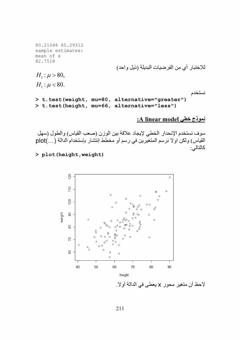
211
80.21048 85.29312 sample estimates: mean of x 82.7518
لإلختبار أي من الفرضيات البديلة (ذيل واحد)
1
1
: 80,
: 80.
H
H
µ
µ
>
<
نستخدم> t.test(weight, mu=80, alternative="greater")
> t.test(height, mu=66, alternative="less")
:A linear modelنموذج خطي
سوف نستخدم اإلنحدار الخطي إليجاد عالقة بين الوزن (صعب القياس) والطول (سهل
(…)plotالقياس) ولكن اوال نرسم المتغيرين في رسم أو مخطط إنتشار بإستخدام الدالة كالتالي:
> plot(height,weight)
يعطى في الدالة أوال. xالحظ أن متغير محور
212
(الحظ أن هذه الدالة مرنة جدا وتستخدم هنا (…)lmلتطبيق نماذج خطية نستخدم الدالة في أبسط أشكالها ولها إستخدامات اخرى نتطرق لها في حينها) لتطبيق إنحدار خطي
بسيط للوزن على الطول> lmres <- lm(weight ~ height)
نالحظ شيئين: ~. الرمز model formulaتسمى صيغة نموذج weight ~ heightالحجة •
فاألمر هنا يطلب نموذج خطي والذي فيه described byيعني " موصوف بـ " الوزن يوصف بالطول سوف نتكلم أكثر عن صيغ النموذج الحقا.
شيئ فقط ظهر محفذ بعد إدخال الدالة بحججها والضغط على إدخال لم يحدث •تعمل بوضع جميع المعلومات في شيئ Rولم تخرج نتائج؟ ذلك ألن <األوامر object يعاد بواسطة الدالةlm(…) وهذا يعرف بإسم شيئ النموذجmodel
object وفي هذا المثال فإننا قمنا بتخزين المعلومات في شيئ نموذج يسمىlmres إستخدام دوال مستخلصة والذي يمكن مشاهدتة وأستخدامه بextractor
functions . أسهل طريقة إلستخالص معلومة هي بطباعة معرف (إسم) شيئ نموذج وفي هذا المثال
lmres كما يمكننا إستخدام الدالةsummary(…) إلعطاء تفصيالت أكثر أو الدالةabline(…) .لتوليد رسم للخط المطبق
> lmres
Call: lm(formula = weight ~ height) Coefficients: (Intercept) height 26.0319 0.8724
> summary(lmres)
Call: lm(formula = weight ~ height) Residuals: Min 1Q Median 3Q Max -23.1146 -6.1125 -0.1758 5.6578 29.1479 Coefficients: Estimate Std. Error t value Pr(>|t|) (Intercept) 26.03185 6.05581 4.299 4.06e-05 *** height 0.87239 0.09204 9.479 1.64e-15 ***
---

213
Signif. codes: 0 ‘***’ 0.001 ‘**’ 0.01 ‘*’ 0.05 ‘.’ 0.1 ‘ ’ 1
Residual standard error: 9.298 on 98 degrees of freedom Multiple R-squared: 0.4783, Adjusted R-squared: 0.473 F-statistic: 89.84 on 1 and 98 DF, p-value: 1.64e-15

214
Quitting and returning to a savedالخروج والعودة لفضاء عمل مخزن workspace:
غير أساسية ثم تخزين فضاء objectsياء قبل إنهاء جلسة من األفضل إزالة أي أش
العمل في دليل العمل الحالي> save.image("sheep2.Rdata")
> quit()
يسأل فيما إذا كان يراد تخزين فضاء العمل ولو وافقنا فإنه Rالحظ عند الخروج فإن
اإلفتراضي ولهذا عند طلب التخزين Rdata.سوف يعيد تخزين فضاء العمل في ملف ).Rض تخزينه مرة أخري (هذا إجراء إختياري في نرف
ونعيد تعريف دليل العمل ثم Rلكي نعود لفضاء العمل الذي تم تخزينه نعيد تشغيل لتحميل فضاء العمل (…)loadنستخدم الدالة
> setwd("C:/orCourse ")
> load("sheep2.Rdata")
> objects()
بقة.نالحظ وجود جميع األشياء من الجلسة السا
:Properties of objectsخواص األشياء
تعطي طول المتجه فمثال (…)lengthالدالة > length(sheep2)
[1] 2 > length(plot)
[1] 1
طول إطار بيانات هو عدد المتغيرات التي يحويها اإلطار. يمكن إيجاد طول دالة ولكن (…)attributesدالة تعطي طور الشيئ بينما ال (…)modeليس له معنى. الدالة
تعطي الصفات غير الجوهرية> mode(sheep2)
[1] "list" > attributes(sheep2)
$names [1] "weight" "height" $class [1] "data.frame" $row.names
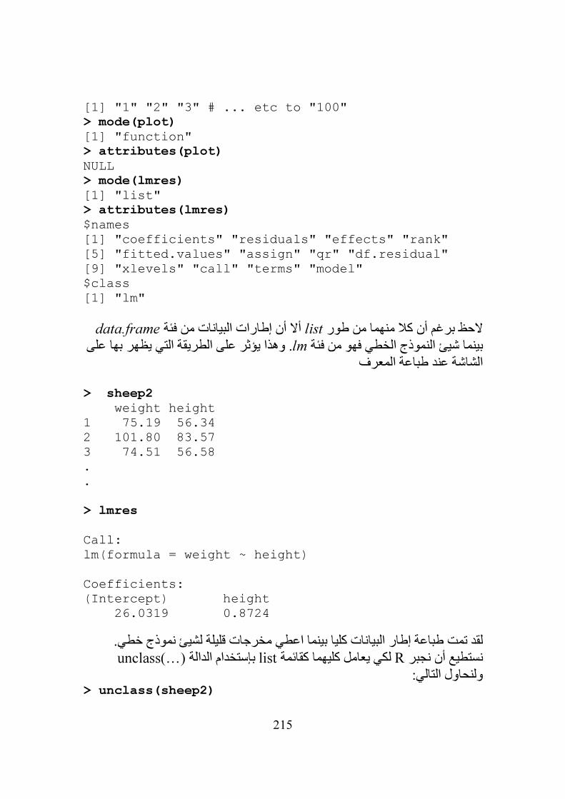
215
[1] "1" "2" "3" # ... etc to "100" > mode(plot)
[1] "function" > attributes(plot)
NULL > mode(lmres)
[1] "list" > attributes(lmres)
$names [1] "coefficients" "residuals" "effects" "rank" [5] "fitted.values" "assign" "qr" "df.residual" [9] "xlevels" "call" "terms" "model" $class [1] "lm"
data.frameأال أن إطارات البيانات من فئة listالحظ برغم أن كال منهما من طور
. وهذا يؤثر على الطريقة التي يظهر بها على lmبينما شيئ النموذج الخطي فهو من فئة الشاشة عند طباعة المعرف
> sheep2
weight height 1 75.19 56.34 2 101.80 83.57 3 74.51 56.58 . . > lmres
Call: lm(formula = weight ~ height) Coefficients: (Intercept) height 26.0319 0.8724
لقد تمت طباعة إطار البيانات كليا بينما اعطي مخرجات قليلة لشيئ نموذج خطي. (…)unclassبإستخدام الدالة listلكي يعامل كليهما كقائمة Rنستطيع أن نجبر ولنحاول التالي:
> unclass(sheep2)
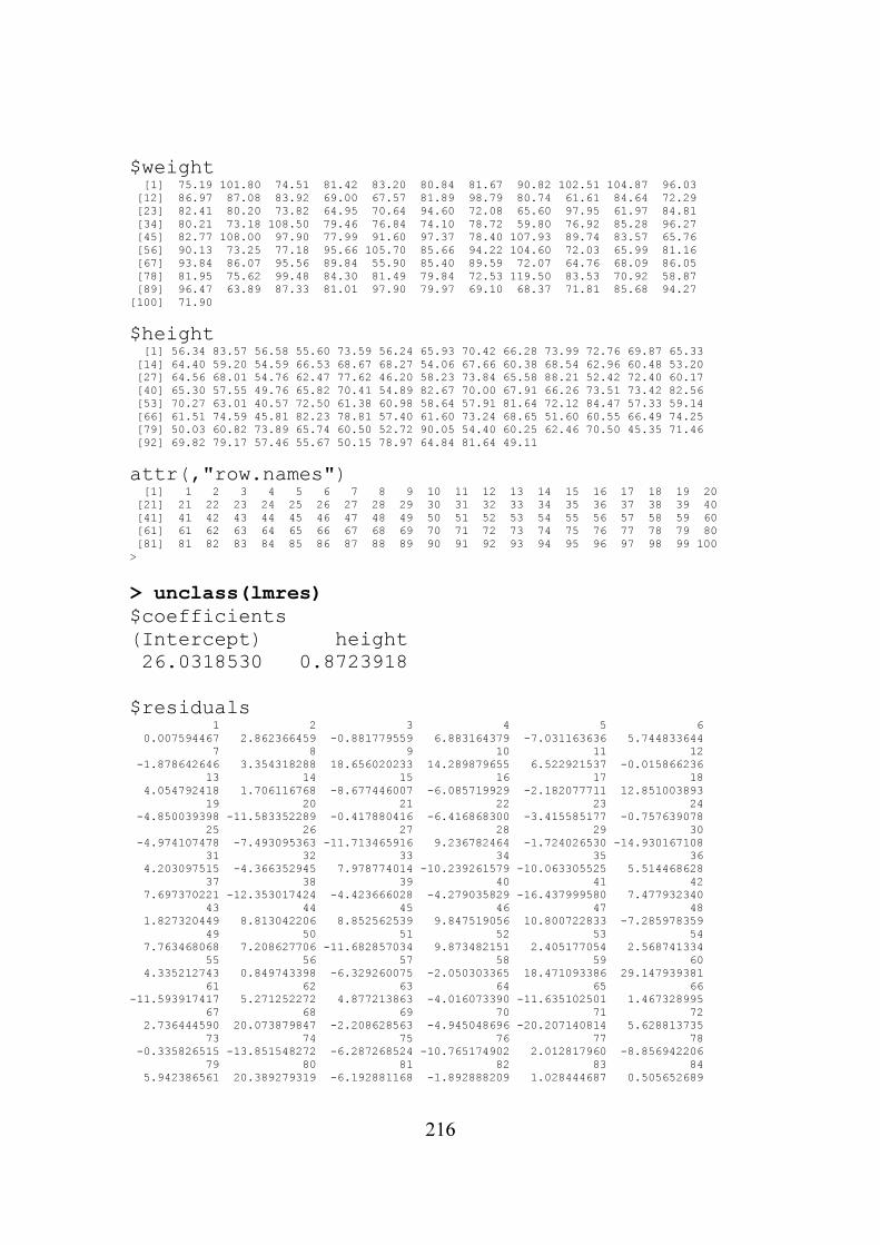
216
$weight [1] 75.19 101.80 74.51 81.42 83.20 80.84 81.67 90.82 102.51 104.87 96.03
[12] 86.97 87.08 83.92 69.00 67.57 81.89 98.79 80.74 61.61 84.64 72.29
[23] 82.41 80.20 73.82 64.95 70.64 94.60 72.08 65.60 97.95 61.97 84.81
[34] 80.21 73.18 108.50 79.46 76.84 74.10 78.72 59.80 76.92 85.28 96.27
[45] 82.77 108.00 97.90 77.99 91.60 97.37 78.40 107.93 89.74 83.57 65.76
[56] 90.13 73.25 77.18 95.66 105.70 85.66 94.22 104.60 72.03 65.99 81.16
[67] 93.84 86.07 95.56 89.84 55.90 85.40 89.59 72.07 64.76 68.09 86.05
[78] 81.95 75.62 99.48 84.30 81.49 79.84 72.53 119.50 83.53 70.92 58.87
[89] 96.47 63.89 87.33 81.01 97.90 79.97 69.10 68.37 71.81 85.68 94.27
[100] 71.90
$height [1] 56.34 83.57 56.58 55.60 73.59 56.24 65.93 70.42 66.28 73.99 72.76 69.87 65.33
[14] 64.40 59.20 54.59 66.53 68.67 68.27 54.06 67.66 60.38 68.54 62.96 60.48 53.20
[27] 64.56 68.01 54.76 62.47 77.62 46.20 58.23 73.84 65.58 88.21 52.42 72.40 60.17
[40] 65.30 57.55 49.76 65.82 70.41 54.89 82.67 70.00 67.91 66.26 73.51 73.42 82.56
[53] 70.27 63.01 40.57 72.50 61.38 60.98 58.64 57.91 81.64 72.12 84.47 57.33 59.14
[66] 61.51 74.59 45.81 82.23 78.81 57.40 61.60 73.24 68.65 51.60 60.55 66.49 74.25
[79] 50.03 60.82 73.89 65.74 60.50 52.72 90.05 54.40 60.25 62.46 70.50 45.35 71.46
[92] 69.82 79.17 57.46 55.67 50.15 78.97 64.84 81.64 49.11
attr(,"row.names") [1] 1 2 3 4 5 6 7 8 9 10 11 12 13 14 15 16 17 18 19 20
[21] 21 22 23 24 25 26 27 28 29 30 31 32 33 34 35 36 37 38 39 40
[41] 41 42 43 44 45 46 47 48 49 50 51 52 53 54 55 56 57 58 59 60
[61] 61 62 63 64 65 66 67 68 69 70 71 72 73 74 75 76 77 78 79 80
[81] 81 82 83 84 85 86 87 88 89 90 91 92 93 94 95 96 97 98 99 100
>
> unclass(lmres)
$coefficients (Intercept) height 26.0318530 0.8723918 $residuals 1 2 3 4 5 6
0.007594467 2.862366459 -0.881779559 6.883164379 -7.031163636 5.744833644
7 8 9 10 11 12
-1.878642646 3.354318288 18.656020233 14.289879655 6.522921537 -0.015866236
13 14 15 16 17 18
4.054792418 1.706116768 -8.677446007 -6.085719929 -2.182077711 12.851003893
19 20 21 22 23 24
-4.850039398 -11.583352289 -0.417880416 -6.416868300 -3.415585177 -0.757639078
25 26 27 28 29 30
-4.974107478 -7.493095363 -11.713465916 9.236782464 -1.724026530 -14.930167108
31 32 33 34 35 36
4.203097515 -4.366352945 7.978774014 -10.239261579 -10.063305525 5.514468628
37 38 39 40 41 42
7.697370221 -12.353017424 -4.423666028 -4.279035829 -16.437999580 7.477932340
43 44 45 46 47 48
1.827320449 8.813042206 8.852562539 9.847519056 10.800722833 -7.285978359
49 50 51 52 53 54
7.763468068 7.208627706 -11.682857034 9.873482151 2.405177054 2.568741334
55 56 57 58 59 60
4.335212743 0.849743398 -6.329260075 -2.050303365 18.471093386 29.147939381
61 62 63 64 65 66
-11.593917417 5.271252272 4.877213863 -4.016073390 -11.635102501 1.467328995
67 68 69 70 71 72
2.736444590 20.073879847 -2.208628563 -4.945048696 -20.207140814 5.628813735
73 74 75 76 77 78
-0.335826515 -13.851548272 -6.287268524 -10.765174902 2.012817960 -8.856942206
79 80 81 82 83 84
5.942386561 20.389279319 -6.192881168 -1.892888209 1.028444687 0.505652689
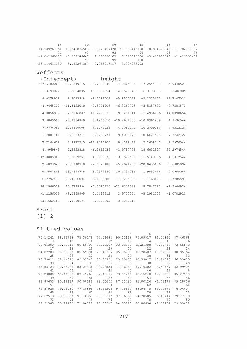
217
85 86 87 88 89 90
14.909267764 10.040034508 -7.673457370 -21.651443190 8.934526946 -1.704819937
91 92 93 94 95 96
-1.042969157 -5.932246647 2.800890265 3.810515680 -5.497903045 -1.412300452
97 98 99 100
-23.114631380 3.082264387 -2.983917417 3.024986993
$effects (Intercept) height -827.5180000 -88.1319145 -0.7006440 7.0875994 -7.2544388 5.9340527
-1.9198022 3.2064095 18.6065394 14.0570945 6.3193795 -0.1506989
4.0278978 1.7013328 -8.5586006 -5.8572723 -2.2375022 12.7447011
-4.9468322 -11.3423040 -0.5001706 -6.3260773 -3.5187972 -0.7281873
-4.8856939 -7.2316007 -11.7220539 9.1461711 -1.4996206 -14.8890656
3.8840095 -3.9384340 8.1206810 -10.4684805 -10.0961439 4.9436046
7.9774093 -12.5480005 -4.3278823 -4.3052172 -16.2799256 7.8212127
1.7887761 8.6653711 9.0738777 9.4083679 10.6627995 -7.3742122
7.7144628 6.9872545 -11.9020905 9.4369462 2.2608345 2.5970044
4.8969843 0.6523828 -6.2622439 -1.9737773 18.6032527 29.2974544
-12.0085805 5.0829261 4.3952679 -3.8527690 -11.5148306 1.5312544
2.4893945 20.5110710 -2.6373188 -5.2924288 -20.0455006 5.6905994
-0.5507805 -13.9573755 -5.9877340 -10.6784256 1.9583444 -9.0959088
6.2792477 20.4696094 -6.4232888 -1.9295306 1.1163827 0.7785593
14.2946579 10.2729994 -7.5795756 -21.6101039 8.7847161 -1.2566924
-1.2156039 -6.0658905 2.4449512 3.9707294 -5.2951323 -1.0782923
-23.4658155 3.0670194 -3.3985805 3.3837210
$rank [1] 2 $fitted.values 1 2 3 4 5 6 7 8
75.18241 98.93763 75.39178 74.53684 90.23116 75.09517 83.54864 87.46568
9 10 11 12 13 14 15 16
83.85398 90.58012 89.50708 86.98587 83.02521 82.21388 77.67745 73.65572
17 18 19 20 21 22 23 24
84.07208 85.93900 85.59004 73.19335 85.05788 78.70687 85.82559 80.95764
25 26 27 28 29 30 31 32
78.79411 72.44310 82.35347 85.36322 73.80403 80.53017 93.74690 66.33635
33 34 35 36 37 38 39 40
76.83123 90.44926 83.24331 102.98553 71.76263 89.19302 78.52367 82.99904
41 42 43 44 45 46 47 48
76.23800 69.44207 83.45268 87.45696 73.91744 98.15248 87.09928 85.27598
49 50 51 52 53 54 55 56
83.83653 90.16137 90.08286 98.05652 87.33482 81.00126 61.42479 89.28026
57 58 59 60 61 62 63 64
79.57926 79.23030 77.18891 76.55206 97.25392 88.94875 99.72279 76.04607
65 66 67 68 69 70 71 72
77.62510 79.69267 91.10356 65.99612 97.76863 94.78505 76.10714 79.77119
73 74 75 76 77 78 79 80
89.92583 85.92155 71.04727 78.85517 84.03718 90.80694 69.67761 79.09072
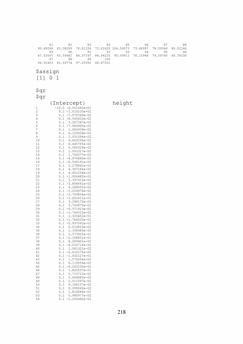
218
81 82 83 84 85 86 87 88
90.49288 83.38289 78.81156 72.02435 104.59073 73.48997 78.59346 80.52144
89 90 91 92 93 94 95 96
87.53547 65.59482 88.37297 86.94225 95.09911 76.15948 74.59790 69.78230
97 98 99 100
94.92463 82.59774 97.25392 68.87501
$assign [1] 0 1 $qr $qr (Intercept) height 1 -10.0 -6.501660e+02
2 0.1 -1.010233e+02
3 0.1 -7.570349e-02
4 0.1 -8.540422e-02
5 0.1 9.267347e-02
6 0.1 -7.906905e-02
7 0.1 1.684939e-02
8 0.1 6.129458e-02
9 0.1 2.031394e-02
10 0.1 9.663295e-02
11 0.1 8.445755e-02
12 0.1 5.585029e-02
13 0.1 1.091017e-02
14 0.1 1.704377e-03
15 0.1 -4.976889e-02
16 0.1 -9.540191e-02
17 0.1 2.278862e-02
18 0.1 4.397184e-02
19 0.1 4.001236e-02
20 0.1 -1.006482e-01
21 0.1 3.397415e-02
22 0.1 -3.808841e-02
23 0.1 4.268501e-02
24 0.1 -1.254976e-02
25 0.1 -3.709854e-02
26 0.1 -1.091611e-01
27 0.1 3.288170e-03
28 0.1 3.743870e-02
29 0.1 -9.371913e-02
30 0.1 -1.740012e-02
31 0.1 1.325652e-01
32 0.1 -1.784520e-01
33 0.1 -5.937063e-02
34 0.1 9.514815e-02
35 0.1 1.338485e-02
36 0.1 2.373925e-01
37 0.1 -1.168821e-01
38 0.1 8.089401e-02
39 0.1 -4.016714e-02
40 0.1 1.061321e-02
41 0.1 -6.610175e-02
42 0.1 -1.432127e-01
43 0.1 1.576054e-02
44 0.1 6.119559e-02
45 0.1 -9.243230e-02
46 0.1 1.825537e-01
47 0.1 5.713712e-02
48 0.1 3.644883e-02
49 0.1 2.011597e-02
50 0.1 9.188157e-02
51 0.1 9.099069e-02
52 0.1 1.814648e-01
53 0.1 5.980977e-02
54 0.1 -1.205482e-02
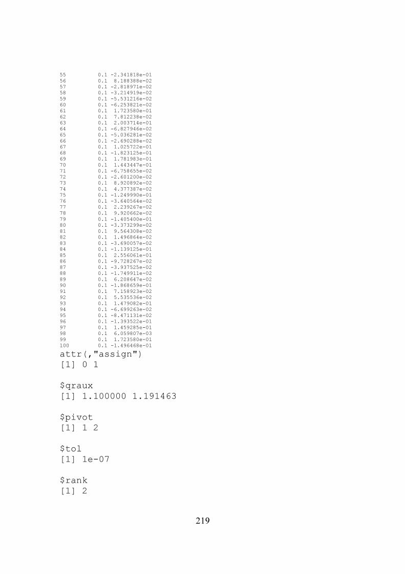
219
55 0.1 -2.341818e-01
56 0.1 8.188388e-02
57 0.1 -2.818971e-02
58 0.1 -3.214919e-02
59 0.1 -5.531216e-02
60 0.1 -6.253821e-02
61 0.1 1.723580e-01
62 0.1 7.812238e-02
63 0.1 2.003714e-01
64 0.1 -6.827946e-02
65 0.1 -5.036281e-02
66 0.1 -2.690288e-02
67 0.1 1.025722e-01
68 0.1 -1.823125e-01
69 0.1 1.781983e-01
70 0.1 1.443447e-01
71 0.1 -6.758655e-02
72 0.1 -2.601200e-02
73 0.1 8.920892e-02
74 0.1 4.377387e-02
75 0.1 -1.249990e-01
76 0.1 -3.640564e-02
77 0.1 2.239267e-02
78 0.1 9.920662e-02
79 0.1 -1.405400e-01
80 0.1 -3.373299e-02
81 0.1 9.564308e-02
82 0.1 1.496864e-02
83 0.1 -3.690057e-02
84 0.1 -1.139125e-01
85 0.1 2.556061e-01
86 0.1 -9.728267e-02
87 0.1 -3.937525e-02
88 0.1 -1.749911e-02
89 0.1 6.208647e-02
90 0.1 -1.868659e-01
91 0.1 7.158923e-02
92 0.1 5.535536e-02
93 0.1 1.479082e-01
94 0.1 -6.699263e-02
95 0.1 -8.471131e-02
96 0.1 -1.393522e-01
97 0.1 1.459285e-01
98 0.1 6.059807e-03
99 0.1 1.723580e-01
100 0.1 -1.496468e-01
attr(,"assign") [1] 0 1 $qraux [1] 1.100000 1.191463 $pivot [1] 1 2 $tol [1] 1e-07 $rank [1] 2
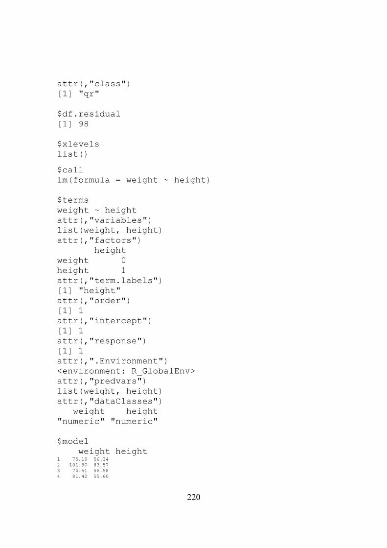
220
attr(,"class") [1] "qr" $df.residual [1] 98 $xlevels list()
$call lm(formula = weight ~ height) $terms weight ~ height attr(,"variables") list(weight, height) attr(,"factors") height weight 0 height 1 attr(,"term.labels") [1] "height" attr(,"order") [1] 1 attr(,"intercept") [1] 1 attr(,"response") [1] 1 attr(,".Environment") <environment: R_GlobalEnv> attr(,"predvars") list(weight, height) attr(,"dataClasses") weight height "numeric" "numeric" $model weight height 1 75.19 56.34
2 101.80 83.57
3 74.51 56.58
4 81.42 55.60
221
5 83.20 73.59
6 80.84 56.24
7 81.67 65.93
8 90.82 70.42
9 102.51 66.28
10 104.87 73.99
11 96.03 72.76
12 86.97 69.87
13 87.08 65.33
14 83.92 64.40
15 69.00 59.20
16 67.57 54.59
17 81.89 66.53
18 98.79 68.67
19 80.74 68.27
20 61.61 54.06
21 84.64 67.66
22 72.29 60.38
23 82.41 68.54
24 80.20 62.96
25 73.82 60.48
26 64.95 53.20
27 70.64 64.56
28 94.60 68.01
29 72.08 54.76
30 65.60 62.47
31 97.95 77.62
32 61.97 46.20
33 84.81 58.23
34 80.21 73.84
35 73.18 65.58
36 108.50 88.21
37 79.46 52.42
38 76.84 72.40
39 74.10 60.17
40 78.72 65.30
41 59.80 57.55
42 76.92 49.76
43 85.28 65.82
44 96.27 70.41
45 82.77 54.89
46 108.00 82.67
47 97.90 70.00
48 77.99 67.91
49 91.60 66.26
50 97.37 73.51
51 78.40 73.42
52 107.93 82.56
53 89.74 70.27
54 83.57 63.01
55 65.76 40.57
56 90.13 72.50
57 73.25 61.38
58 77.18 60.98
59 95.66 58.64
60 105.70 57.91
61 85.66 81.64
62 94.22 72.12
63 104.60 84.47
64 72.03 57.33
65 65.99 59.14
66 81.16 61.51
67 93.84 74.59
68 86.07 45.81
69 95.56 82.23
70 89.84 78.81
71 55.90 57.40
72 85.40 61.60
73 89.59 73.24
74 72.07 68.65
75 64.76 51.60

222
76 68.09 60.55
77 86.05 66.49
78 81.95 74.25
79 75.62 50.03
80 99.48 60.82
81 84.30 73.89
82 81.49 65.74
83 79.84 60.50
84 72.53 52.72
85 119.50 90.05
86 83.53 54.40
87 70.92 60.25
88 58.87 62.46
89 96.47 70.50
90 63.89 45.35
91 87.33 71.46
92 81.01 69.82
93 97.90 79.17
94 79.97 57.46
95 69.10 55.67
96 68.37 50.15
97 71.81 78.97
98 85.68 64.84
99 94.27 81.64
100 71.90 49.11
>
sheep2يشبه مخرجات unclass(lmres) <الحظ أن الجزء األخير من والذي هو إطار بيانات مكون من متغيرات (model$)يحوي صفة lmresوذلك ألن
(…)classيع إيجاد فئة أي شيئ مستخدمين الدالة نحن نضعها في النموذج. نستط
> class(lmres$model)
[1] "data.frame"
هو طريقة مريحة إلخفاء حقيقة معقدة. في الحقيقة modeوهذه ليست النهاية ألن الطور R تعمل على نوعtype الشيئ وفي بعض األحيان يكون نوع أكثر تحديدا ودقة من
ت اخرى فإن الخاصيتين متطابقة. نستطيع إيجاد نوع شيئ ولكن في حاال modeطور والطريقة التي تخزن بها تعطى بالدالة (…)typeofبإستخدام الدالة
storage.mode(…) :كالتالي > typeof(sheep2)
[1] "list" > typeof(sheep2$weight)
[1] "double" > z <- 1 + 1i
> typeof(z)
[1] "complex" > typeof(plot)
[1] "closure" > storage.mode(plot)
[1] "function"
بعض الدوال:
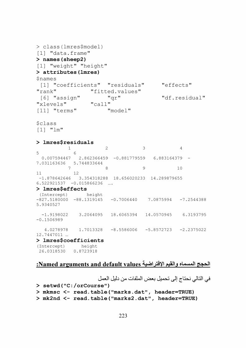
223
> class(lmres$model) [1] "data.frame" > names(sheep2)
[1] "weight" "height" > attributes(lmres)
$names [1] "coefficients" "residuals" "effects" "rank" "fitted.values" [6] "assign" "qr" "df.residual" "xlevels" "call" [11] "terms" "model" $class [1] "lm" > lmres$residuals 1 2 3 4 5 6 0.007594467 2.862366459 -0.881779559 6.883164379 -7.031163636 5.744833644 7 8 9 10 11 12 -1.878642646 3.354318288 18.656020233 14.289879655 6.522921537 -0.015866236 ….
> lmres$effects (Intercept) height -827.5180000 -88.1319145 -0.7006440 7.0875994 -7.2544388 5.9340527 -1.9198022 3.2064095 18.6065394 14.0570945 6.3193795 -0.1506989 4.0278978 1.7013328 -8.5586006 -5.8572723 -2.2375022 12.7447011 …
> lmres$coefficients (Intercept) height 26.0318530 0.8723918
:Named arguments and default valuesالحجج المسماه والقيم اإلفتراضية
في التالي نحتاج إلى تحميل بعض الملفات من دليل العمل
> setwd("C:/orCourse")
> mkmsc <- read.table("marks.dat", header=TRUE)
> mk2nd <- read.table("marks2.dat", header=TRUE)
224
> attach(mk2nd)
الدوال التالية Rفي لغة > plot(exam1, exam2)
> plot(exam2, exam1)
بينما الثانية تعكس yعلى محور exam 2و xعلى محور exam1االولى ترسم
.Rفي defaultالرسم وهذا هو اإلختيار اإلفتراضي كالتالي named argumentsمسماة لتغيير اإلختيار اإلفتراضي نستخدم حجج
> plot(y=exam2, x=exam1)
> plot(x=exam1, y=exam2)
وكالهما يعطي الرسم نفسه. الحجج المسماه تفيد أكثر في عدم اإللتزام بالترتيب أو القيم
اإلفتراضية فمثال> t.test(exam1)
> t.test(exam1, mu=30)
> t.test(exam1, alternative="greater")
> t.test(exam1, mu=31.5, alternative="less")
> t.test(mu=30, exam1)
> t.test(x=exam1, mu=30)
= alternativeهي الصفر. و t.testفي muالحظ أن القيمة اإلفتراضية لـ
"two.sided"
:namesالصفة
أسماء المتغيرات في والتي تشير إلى namesكما ذكرنا سابقا إطارات البيانات لها صفة (…)namesذلك اإلطار. ويمكن سرد األسماء بإستخدام الدالة
> names(mkmsc)
[1] "courseA" "courseB" "courseC"
sub-objectشيئ - هو تمكيننا من الوصول مباشرة إلى جزء $الغرض من العامل شيئ عن -ويمكننا تغيير األسماء والمحتويات للجزء (…)namesمسرد بواسطة
courseCو courseBو courseAطريق اإلسناد فلنفترض اننا نريد تغيير or342و or241و or221باألسماء التالية

225
> names(mkmsc) <- c("or221", "or241", "or342")
> names(mkmsc)
[1] "or221" "or241" "or342" > mkmsc$or221
[1] 52 71 44 90 23 66
لكل قيمة 2ونستطيع إضافة > mkmsc$or221 <- mkmsc$or221 + 2
> mkmsc$or221
[1] 54 73 46 92 25 68
226
:intrinsic attributes-Other nonصفات غير جوهرية أخرى
الصفات غير الجوهرية األخرى يمكن تغييرها بأإلسناد فمثال في إطار بيانات نريد تغيير و الخ إلى أسماء ذات معنى 3و 2و 1أسماء األسطر اإلفتراضية والتي هي غالبا
> row.names(mkmsc)
[1] "1" "2" "3" "4" "5" "6" > row.names(mkmsc) <- c("Ali", "Badr", "Ahmad", +"Bakur", "Saeed", +"Faris") > mkmsc
or221 or241 or342 Ali 54 67 71 Badr 73 80 84 Ahmad 46 55 55 Bakur 92 76 68 Saeed 25 49 52 Faris 68 61 61 >
يكمل السطر الطويل إلى السطر التالي بوضع عالمة + في بداية السطر Rمالحظة: في التالي.
:Regular sequencesالمتتابعات المنسقة
والتي تتبع نمط او نسق ثابت المتتابعات المنسقة هي متتابعات من األعداد أو الحروف
وهي مفيدة في إختيار أجزاء من متجة وفي توليد قيم للمتغيرات الوصفية. هناك عدة :sequence generatorطرق لتوليد متتابعات منها مولد متتابعة
> 1:10 [1] 1 2 3 4 5 6 7 8 9 10 > 10:1 [1] 10 9 8 7 6 5 4 3 2 1 > 2*1:10 [1] 2 4 6 8 10 12 14 16 18 20 > 1:10 + 1:20 [1] 2 4 6 8 10 12 14 16 18 20 12 14 16 18 20 22 24 26 28 30 > 1:10-1 [1] 0 1 2 3 4 5 6 7 8 9 > 1:(10-1)
227
[1] 1 2 3 4 5 6 7 8 9
الحظ أن ( : ) له افضلية على العملية الحسابية. البناء التاليتعطي مقدار اكبر من المرونة في توليد متتابعات ولها seqالدالة
seq(from, to, by, length, along)
عدد lengthتدل على مقدار الزيادة و byمفسرة ذاتيا الحجة toو fromالحجج
الوحدات في المتتابعة. الحظ انه التستخدم جميع هذه الحجج معا وإال سيسبب هذا في كر والذي طوله هو تسمح لمتجه يذ alongزيادة في التعيين وينتج عنه خطأ. الحجة
الطول المطلوب للمتتابعة > seq(1,10)
[1] 1 2 3 4 5 6 7 8 9 10 > seq(to=10, from=1)
[1] 1 2 3 4 5 6 7 8 9 10 > seq(1,10,by=0.5)
[1] 1.0 1.5 2.0 2.5 3.0 3.5 4.0 4.5 5.0 5.5 6.0 6.5 7.0 7.5 8.0 [16] 8.5 9.0 9.5 10.0 > seq(1,10,length=19)
[1] 1.0 1.5 2.0 2.5 3.0 3.5 4.0 4.5 5.0 5.5 6.0 6.5 7.0 7.5 8.0 [16] 8.5 9.0 9.5 10.0 > seq(1,10,length=19,by=0.25)
Error in seq.default(1, 10, length = 19, by = 0.25) : Too many arguments > seq(1,by=2,length=6)
[1] 1 3 5 7 9 11 > seq(to=30,length=13)
[1] 18 19 20 21 22 23 24 25 26 27 28 29 30 > seq(to=30)
[1] 1 2 3 4 5 6 7 8 9 10 11 12 13 14 15 16 17 18 19 20 21 22 23 24 25 [26] 26 27 28 29 30
تولد متتابعات بتكرارات معينة repالدالة > rep(1, times = 3)
[1] 1 1 1 > rep((1:3), each =5)
[1] 1 1 1 1 1 2 2 2 2 2 3 3 3 3 3

228
:Logical vectorsالمتجهات المنطقية
FALSEو TRUEهي Rالقيم المنطقية في
ألكبرمن =<ألكبر من و <لعدم المساواة و =!للمساواة و ==المقارنة تعمل بإستخدام ألقل من أو يساوي =>ألقل من و >أو يساوي و
NOTلـ ! و ORلـ |و ANDلـ &العمال المنطقية
> tf1 <- c(TRUE,TRUE,FALSE,FALSE)
> tf2 <- c(TRUE,FALSE,TRUE,FALSE)
> tf1 & tf2
[1] TRUE FALSE FALSE FALSE > tf1 | tf2
[1] TRUE TRUE TRUE FALSE > (tf1 & !tf2) | (!tf1 & tf2)
[1] FALSE TRUE TRUE FALSE
Indexing vectors and subsetتأشير متجه وإختيار مجموعة جزئية selection:
أحيانا نرغب في إستخدام جزء من البيانات أو مجموعة جزئية والتي تحقق شرط معين
subscriptingبعامل التذيل لكي تؤشر لجزء من المتجه ويعرف [ ]ولذلك تستخدم
operator والمتجه مابين القوسين يعرف بإسم متجه التأشيرindexing vector فإذاكان متجه التأشير له قيم صحيحة (غالبا متتابعة متسقة) فإن العناصر المؤشرة التابعة
ناصر في المقدمة فعندئذ كل الع -لقيم المتجة المؤشر يتم إختيارها وإذا وجدت عالمه ماعدى الذين تم تأشيرهم سيتم إختيارهم
> attach(mkmsc)
> or221
[1] 54 73 46 92 25 68 > or221[c(1,2,6)]
[1] 54 73 68 > or221[1:4]
[1] 54 73 46 92 > or221[-(1:4)]
[1] 25 68 > or221[seq(6,by=-2)]
[1] 68 92 73

229
> or221[rep((1:3),each=2)]
[1] 54 54 73 73 46 46 > row.names(mkmsc)[1:3]
[1] "Ali" "Badr" "Ahmad"
نالحظ أننا نستطيع عمل التالي: 70التي أعلى من or221إيجاد عالمات الطالب في • or241في 65والذين حصلوا على أقل من or221عالمات طالب • 200عالمات الطالب الذين مجموع عالماتهم الكلي أقل من •
> or221[or221>70]
[1] 73 92 > or241[or221<65]
[1] 67 55 49 > or342[(or221+or241+or342)<200]
[1] 71 55 52 61 > or342[or221>50 & or241>50 & or342>50]
[1] 71 84 68 61
التالي يستخرج األسماء بدل العالمات
> row.names(mkmsc)[or221>70]
[1] "Badr" "Bakur" > row.names(mkmsc)[or241<50 | or221<50 | or342<50]
[1] "Ahmad" "Saeed" > names(mkmsc)[c(sum(or221), sum(or241), sum(or342)) > 350] [1] "or221" "or241" "or342"
:Character sequencesمتتابعات الحروف أو النصوص
)لنفترض أنه لدينا أزواج من النقاط ) ( ) ( ){ }1 1 2 2 5 5
, , , , , ,x y x y x y… يلها ونريد تمث
. characterوالتي تجمع الحجج وتعيد حرف (…)pasteلذلك نستخدم الدالة Rفي لتحديد مانريد إدخاله بين الحجج sepالحجة
> paste(c("x","y"), rep(1:5,each=2), sep="")
[1] "x1" "y1" "x2" "y2" "x3" "y3" "x4" "y4" "x5" "y5" > str1 <- paste("(x", 1:5, sep="")

230
> str2 <- paste("y", 1:5, ")", sep="")
> label1 <- paste(str1,str2,sep=",")
> label1
[1] "(x1,y1)" "(x2,y2)" "(x3,y3)" "(x4,y4)" "(x5,y5)" > mode(label1)
[1] "character"
:Listsالقوائم
كمكونات القائمة هي مجموعة مرتبة من األشياء. األشياء الموجودة في قائمة يشار إليهاcomponents وهذه المكونات قد تكون من أطوار مختلفة. تولد القوائم بإستخدام الدلة
list(…) والقيمة المرجعة هي قائمة بمكونات من الحجج التي اعطيت للقائمة
> mklst <- list("BSc exam marks", c(10,6,2005),
mkmsc)
> mode(mklst)
[1] "list" > length(mklst)
[1] 3 > mklst
[[1]] [1] "BSc exam marks" [[2]] [1] 10 6 2005 [[3]] or221 or241 or342 Ali 54 67 71 Badr 73 80 84 Ahmad 46 55 55 Bakur 92 76 68 Saeed 25 49 52 Faris 68 61 61
للوصول إلى أجزاء من القائمة [ ]دام عامل التأشير نستطيع اآلن إستخ
> mklst[2]

231
[[1]] [1] 10 6 2005
> mode(mklst[2])
[1] "list" > length(mklst[2])
[1] 1
إلى 4الحظ أن نتيجة إستخدام التأشير على قائمة هو قائمة أخرى. إذا أردنا أن نضيف ليست قيمة عددية mklst[2] ألن [ ]يوم فإننا النستطيع أن نستخدم
> mklst[2]+c(4,0,0)
Error in mklst[2] + c(4, 0, 0) : non-numeric argument to binary operator
مثل [[ ]]ولكي نتجنب هذا الخطأ نستخدم أقواس مضاغفة
> mklst[[2]]
[1] 10 6 2005 > mode(mklst[[2]])
[1] "numeric" > mklst[[2]] <- mklst[[2]] + c(4,0,0)
> mklst
متجه عددي فإننا نستطيع إستخدام أي عنصر mklst[[2]]في الحقيقة بما أن إليه 4فيه مباشرة ونضيف
> mklst[[2]][1] <- mklst[[2]][1] + 4
يعيد عنصر من [[ ]]إذا طبق على قائمة فإنه يعيد قائمة والعامل [ ]الحظ أن العامل
اإلفتراضية لعناصر labelلمعادة هو طور العنصر. العالمات القائمة وطور القيمة او ... والتوضح ماتحويه القائمة ويكون علينا تذكر إسم كل عنصر 3و 2و 1قائمة هي
في القائمة وهذا سهال لقوائم تحوي عنصر أو عنصرين ولكن للقوائم التي تحوي عدد اصر وترتيبها في القائمة لهذا كبير من العناصر يكون من الصعب تذكر أسماء كل العن
من اإلفضل إعطاء أسماء لعناصر القائمة مثال كالتالي
> names(mklst) <- c("title", "date", "marks")
$أو العامل [[ ]]ويمكننا اآلن اإلشارة إلى عناصر القائمة إما بإستخدام العامل

232
> mklst[[2]]
[1] 18 6 2005 > mklst[["date"]]
[1] 18 6 2005 > mklst$date
[1] 18 6 2005
نستطيع اإلشارة إلى إسم مباشرة والنحتاج إلستخدام "". كما $الحظ بإستخدامنا للعامل
يمكن إعطاء األسماء عند تعريف القائمة مثل
> mklst <- list("title"="MSc exam marks",
+"date"=c(10,6,2005),
+ "marks"=mkmsc)
:Rيطة في الرسومات البس
مقدرات رسم قوية ومرنة. سوف نستعرض هنا بعضا من هذه المقدرات. Rتمتلك
بعض الرسومات الوصفية:
(…)histسوف نقوم برسم المدرج التكراري ألحد المتغيرات وذلك بإستخدام الدالة كالتالي:
أوال نحدد دليل العمل ونقرأ ملف البيانات> setwd("C:/orCourse")
> mk2nd <- read.table("marks2.dat", header=TRUE)
> attributes(mk2nd)
$names [1] "candno" "exam1" "exam2" "exam3" $class [1] "data.frame" $row.names [1] 1 2 3 4 5 6 7 8 9 10 11 12 13 14 15 16 17 18 19 20 21 22 [23] 23 24 25 26 27 28 29 30 31 32 33 34 35 36 37 38 39 40 41 42 43 44 [45] 45 46 47 48 49 50 51 52 53 54 55
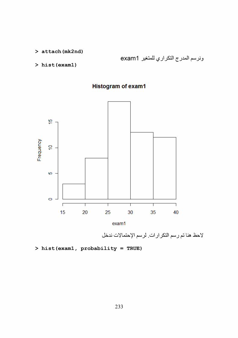
233
> attach(mk2nd)
exam1ونرسم المدرج التكراري للمتغير > hist(exam1)
الحظ هنا تم رسم التكرارات. لرسم اإلحتماالت ندخل
> hist(exam1, probability = TRUE)
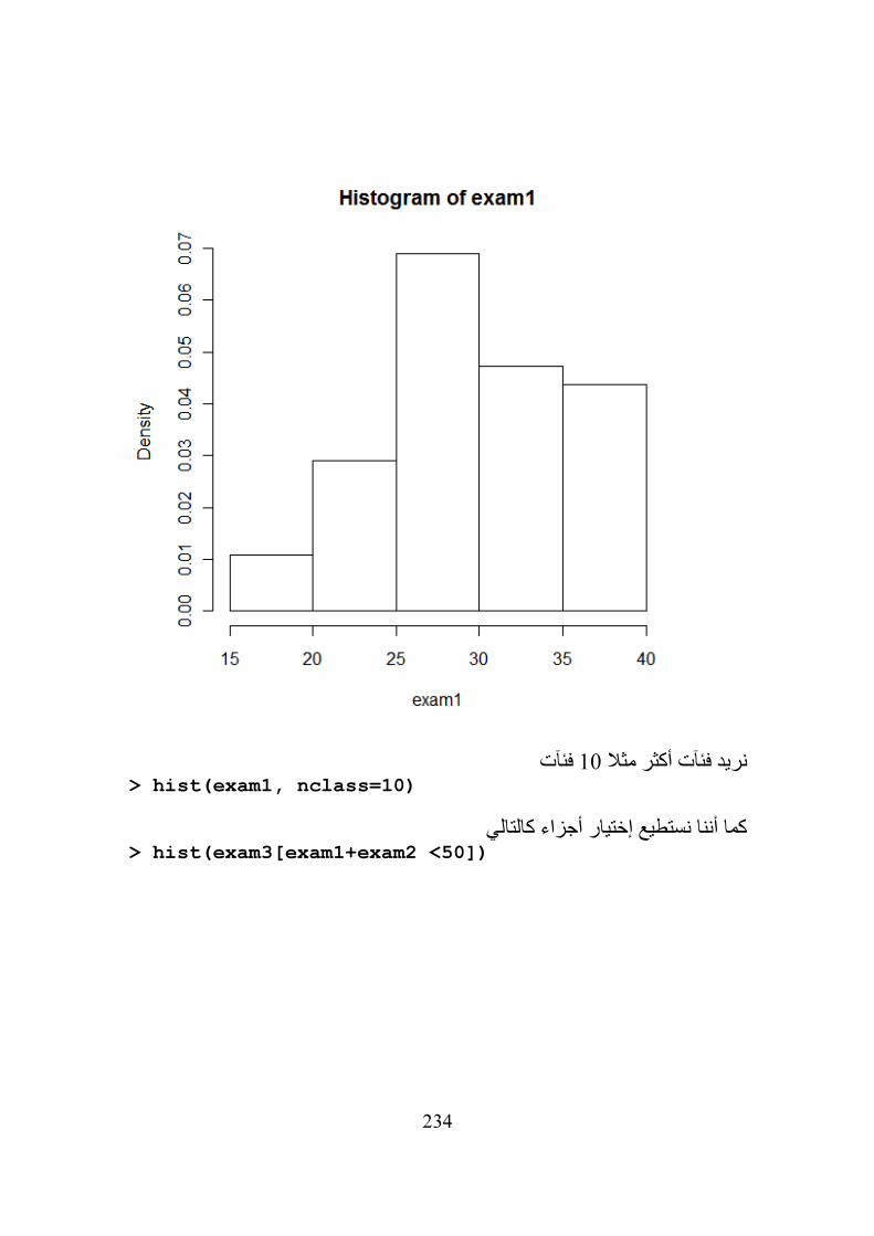
234
فئآت 10نريد فئآت أكثر مثال > hist(exam1, nclass=10)
كما أننا نستطيع إختيار أجزاء كالتالي> hist(exam3[exam1+exam2 <50])
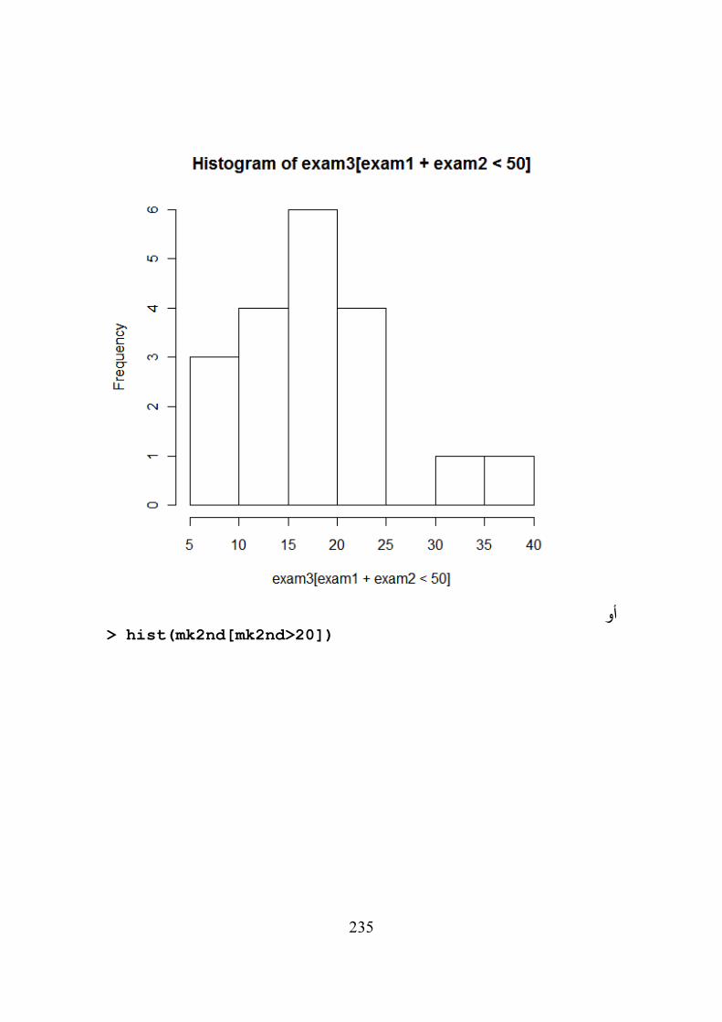
235
أو> hist(mk2nd[mk2nd>20])
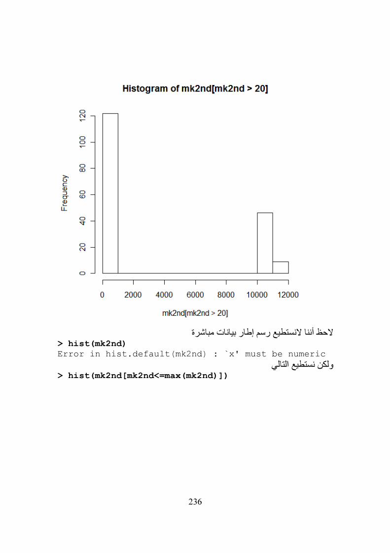
236
الحظ أننا النستطيع رسم إطار بيانات مباشرة
> hist(mk2nd)
Error in hist.default(mk2nd) : `x' must be numeric
ولكن نستطيع التالي> hist(mk2nd[mk2nd<=max(mk2nd)])
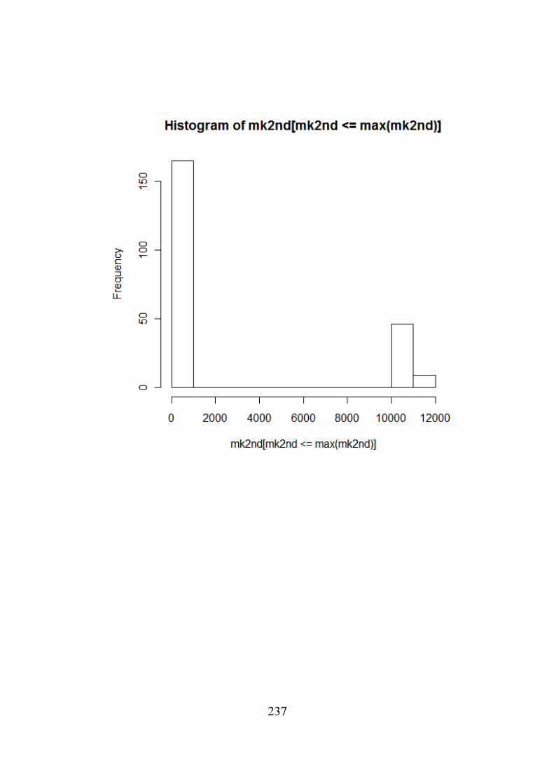
237
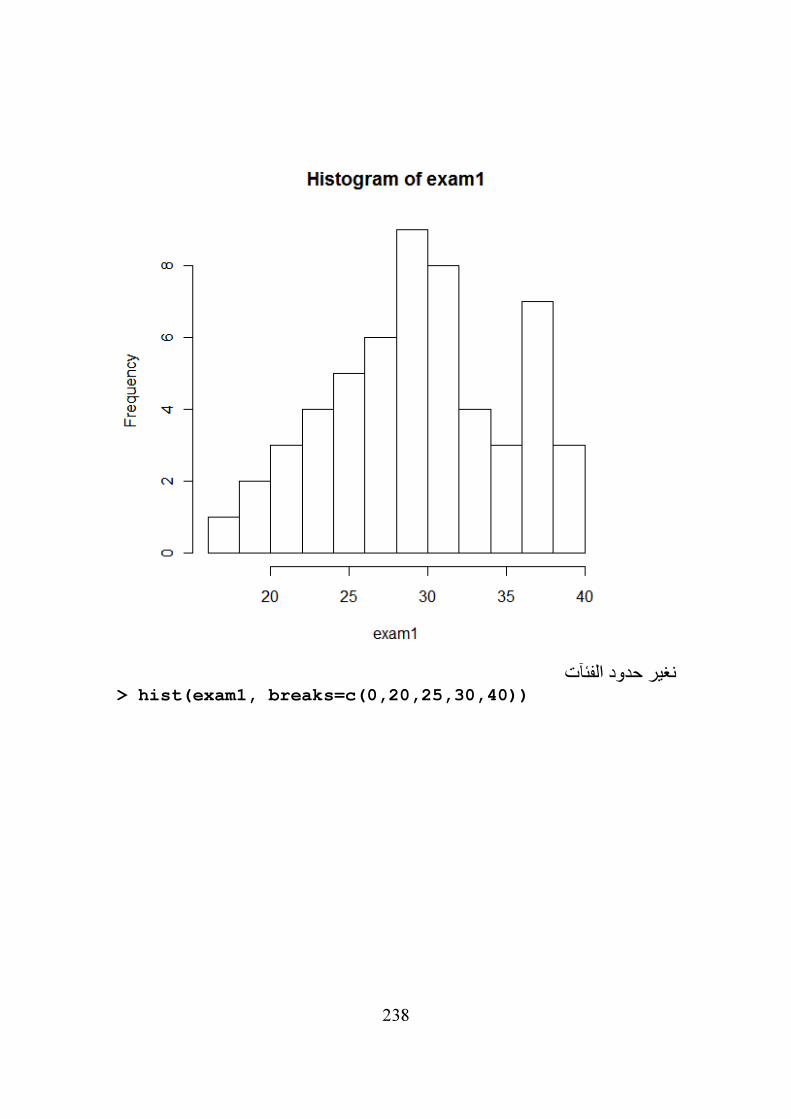
238
نغير حدود الفئآت
> hist(exam1, breaks=c(0,20,25,30,40))
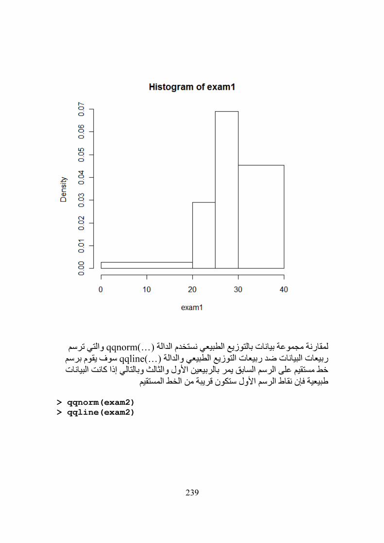
239
والتي ترسم (…)qqnormلمقارنة مجموعة بيانات بالتوزيع الطبيعي نستخدم الدالة سوف يقوم برسم (…)qqlineربيعات البيانات ضد ربيعات التوزيع الطبيعي والدالة
خط مستقيم على الرسم السابق يمر بالربيعين األول والثالث وبالتالي إذا كانت البيانات رسم األول ستكون قريبة من الخط المستقيمطبيعية فإن نقاط ال
> qqnorm(exam2)
> qqline(exam2)
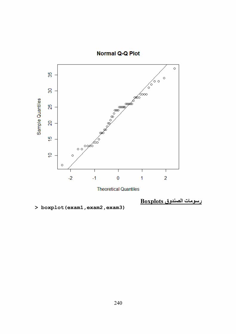
240
Boxplotsرسومات الصندوق
> boxplot(exam1,exam2,exam3)
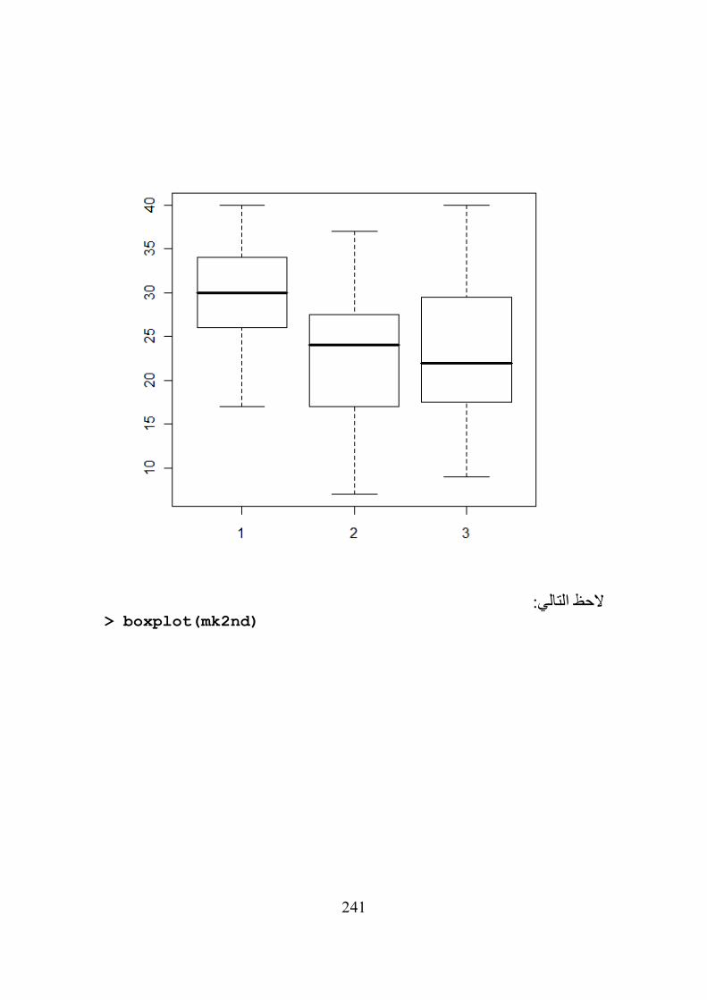
241
الحظ التالي:
> boxplot(mk2nd)
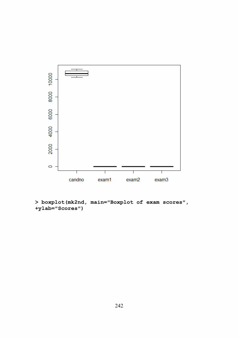
242
> boxplot(mk2nd, main="Boxplot of exam scores",
+ylab="Scores")
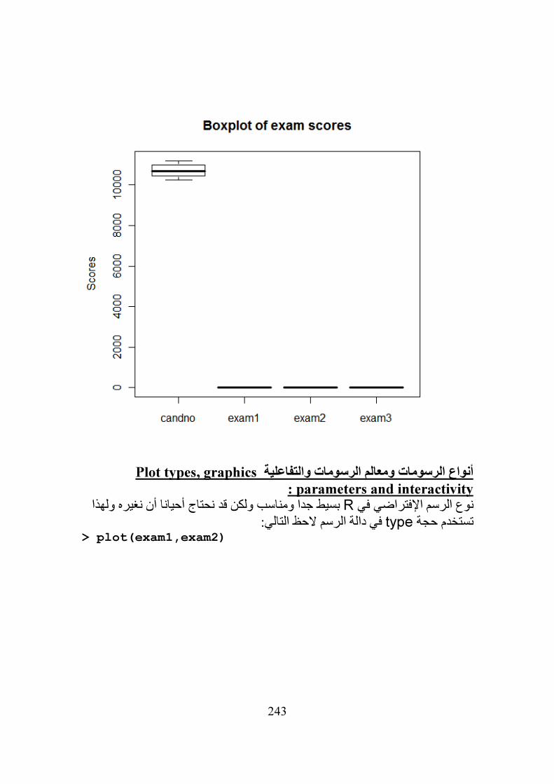
243
Plot types, graphicsمات والتفاعلية أنواع الرسومات ومعالم الرسو
parameters and interactivity : بسيط جدا ومناسب ولكن قد نحتاج أحيانا أن نغيره ولهذا Rنوع الرسم اإلفتراضي في
في دالة الرسم الحظ التالي: typeتستخدم حجة > plot(exam1,exam2)
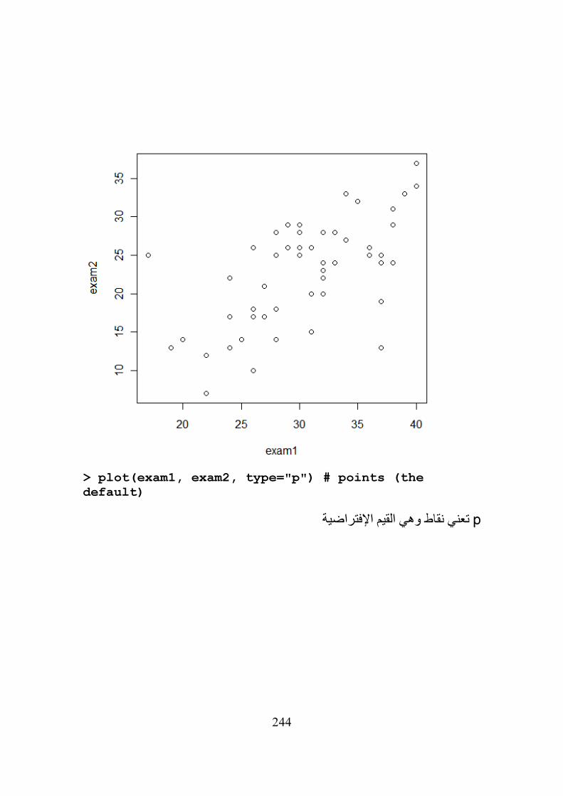
244
> plot(exam1, exam2, type="p") # points (the
default)
p تعني نقاط وهي القيم اإلفتراضية
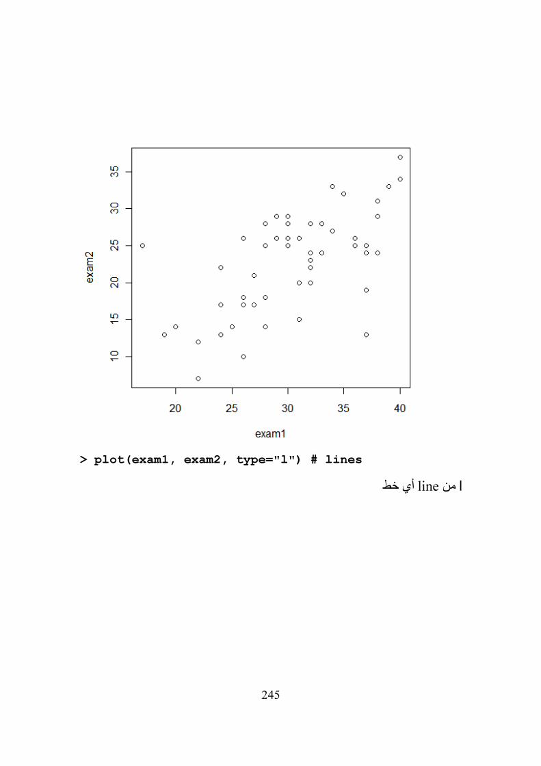
245
> plot(exam1, exam2, type="l") # lines
l منline أي خط
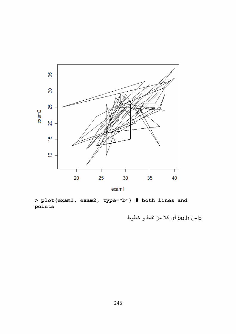
246
> plot(exam1, exam2, type="b") # both lines and
points
b منboth أي كال من نقاط و خطوط
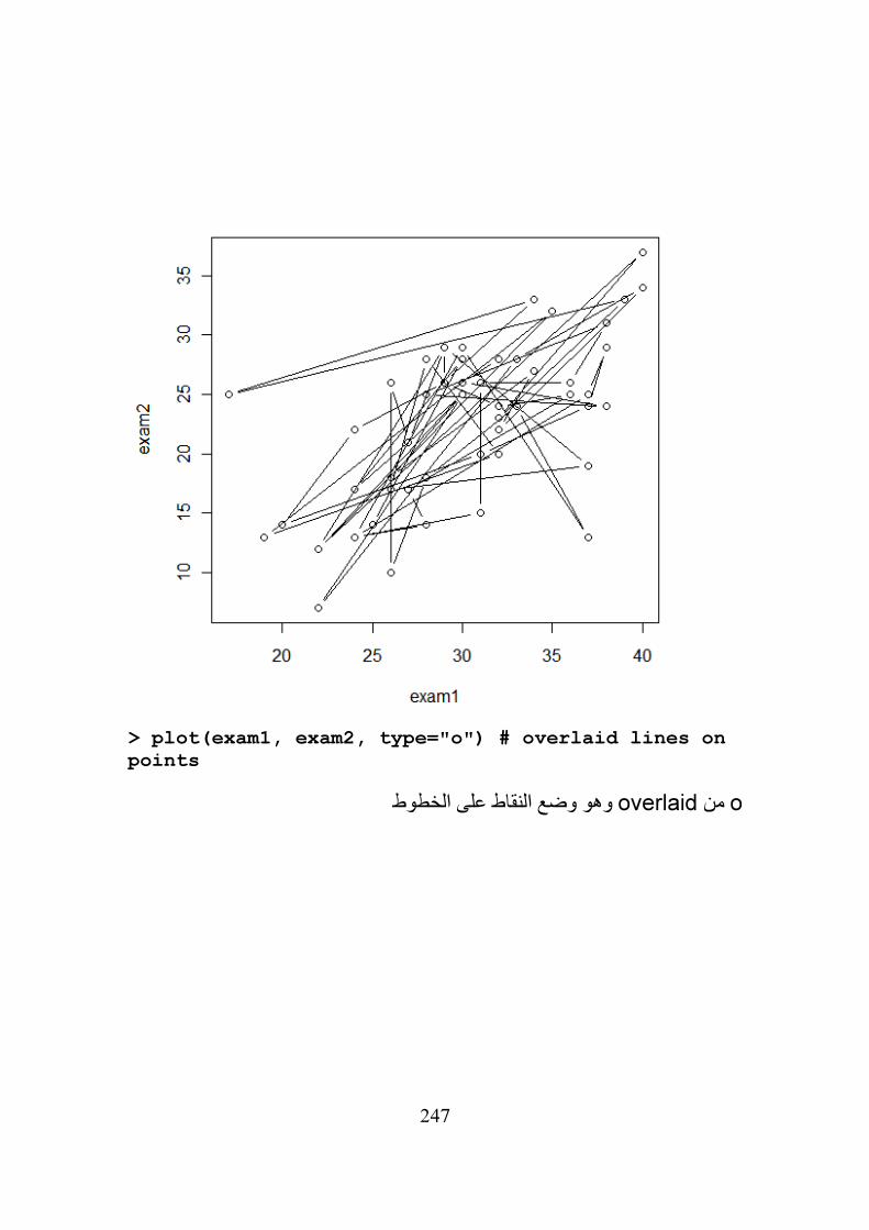
247
> plot(exam1, exam2, type="o") # overlaid lines on
points
o منoverlaid وهو وضع النقاط على الخطوط
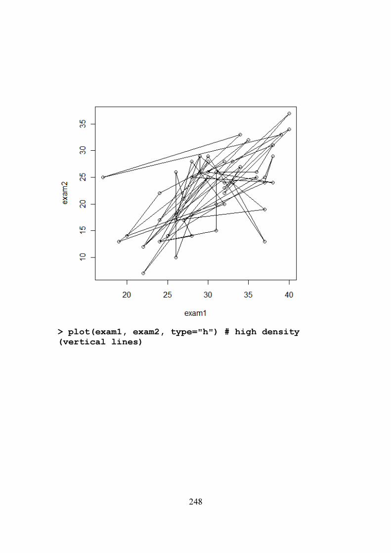
248
> plot(exam1, exam2, type="h") # high density
(vertical lines)
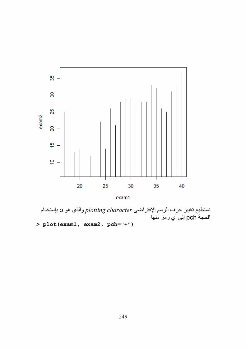
249
بإستخدام oوالذي هو plotting characterنستطيع تغيير حرف الرسم اإلفتراضي
إلى أي رمز منها pchالحجة > plot(exam1, exam2, pch="+")
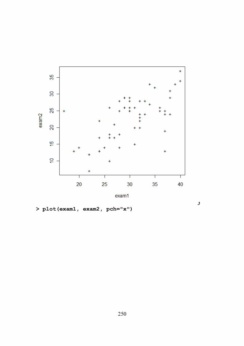
250
و> plot(exam1, exam2, pch="x")
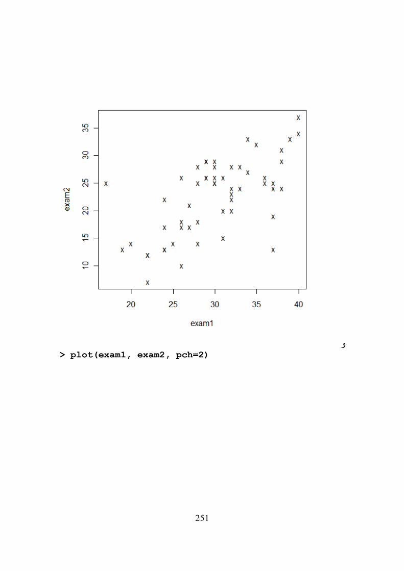
251
و
> plot(exam1, exam2, pch=2)
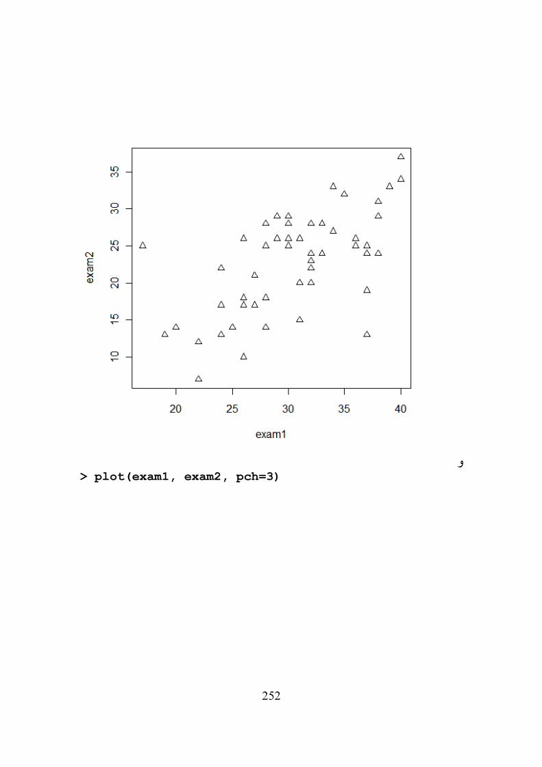
252
و
> plot(exam1, exam2, pch=3)
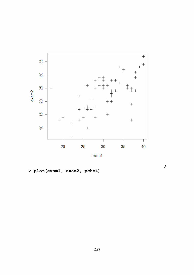
253
و
> plot(exam1, exam2, pch=4)
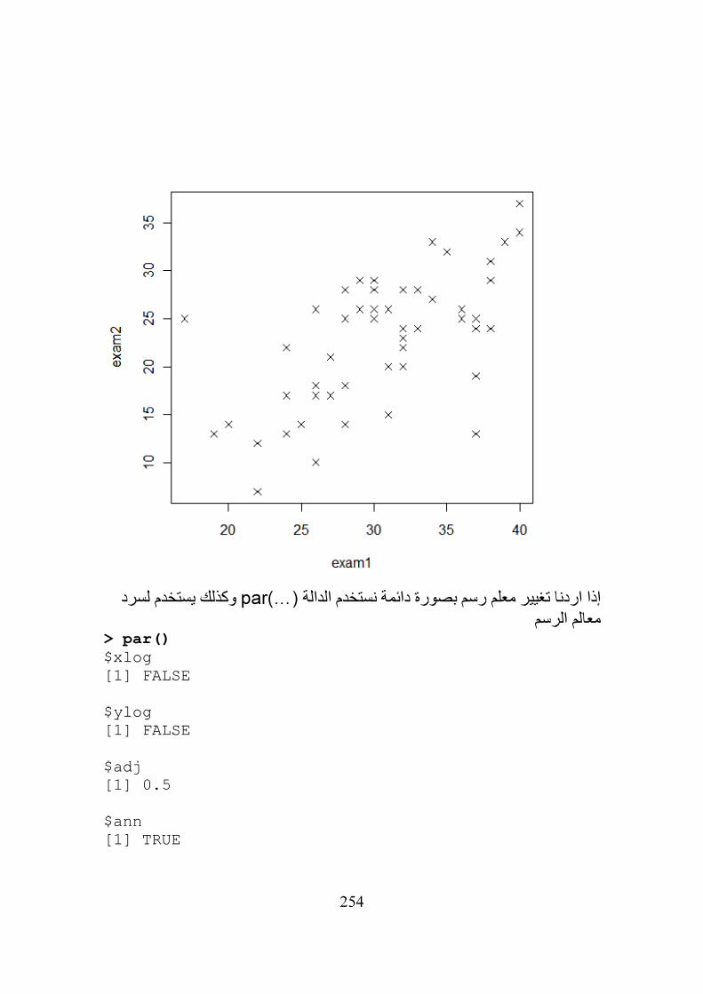
254
وكذلك يستخدم لسرد (…)parإذا اردنا تغيير معلم رسم بصورة دائمة نستخدم الدالة
معالم الرسم> par()
$xlog [1] FALSE $ylog [1] FALSE $adj [1] 0.5 $ann [1] TRUE

255
$ask [1] FALSE $bg [1] "transparent" $bty [1] "o" $cex [1] 1 $cex.axis [1] 1 $cex.lab [1] 1 $cex.main [1] 1.2 $cex.sub [1] 1 $cin [1] 0.15 0.20 $col [1] "black" $col.axis [1] "black" $col.lab [1] "black" $col.main [1] "black" $col.sub
256
[1] "black" $cra [1] 14.4 19.2 $crt [1] 0 $csi [1] 0.2 $cxy [1] 0.03437083 0.05328007 $din [1] 5.604166 5.593749 $err [1] 0 $family [1] "" $fg [1] "black" $fig [1] 0 1 0 1 $fin [1] 5.604166 5.593749 $font [1] 1 $font.axis [1] 1 $font.lab [1] 1
257
$font.main [1] 2 $font.sub [1] 1 $lab [1] 5 5 7 $las [1] 0 $lend [1] "round" $lheight [1] 1 $ljoin [1] "round" $lmitre [1] 10 $lty [1] "solid" $lwd [1] 1 $mai [1] 1.02 0.82 0.82 0.42 $mar [1] 5.1 4.1 4.1 2.1 $mex [1] 1
258
$mfcol [1] 1 1 $mfg [1] 1 1 1 1 $mfrow [1] 1 1 $mgp [1] 3 1 0 $mkh [1] 0.001 $new [1] FALSE $oma [1] 0 0 0 0 $omd [1] 0 1 0 1 $omi [1] 0 0 0 0 $pch [1] 1 $pin [1] 4.364166 3.753749 $plt [1] 0.1463197 0.9250557 0.1823464 0.8534078 $ps [1] 12 $pty
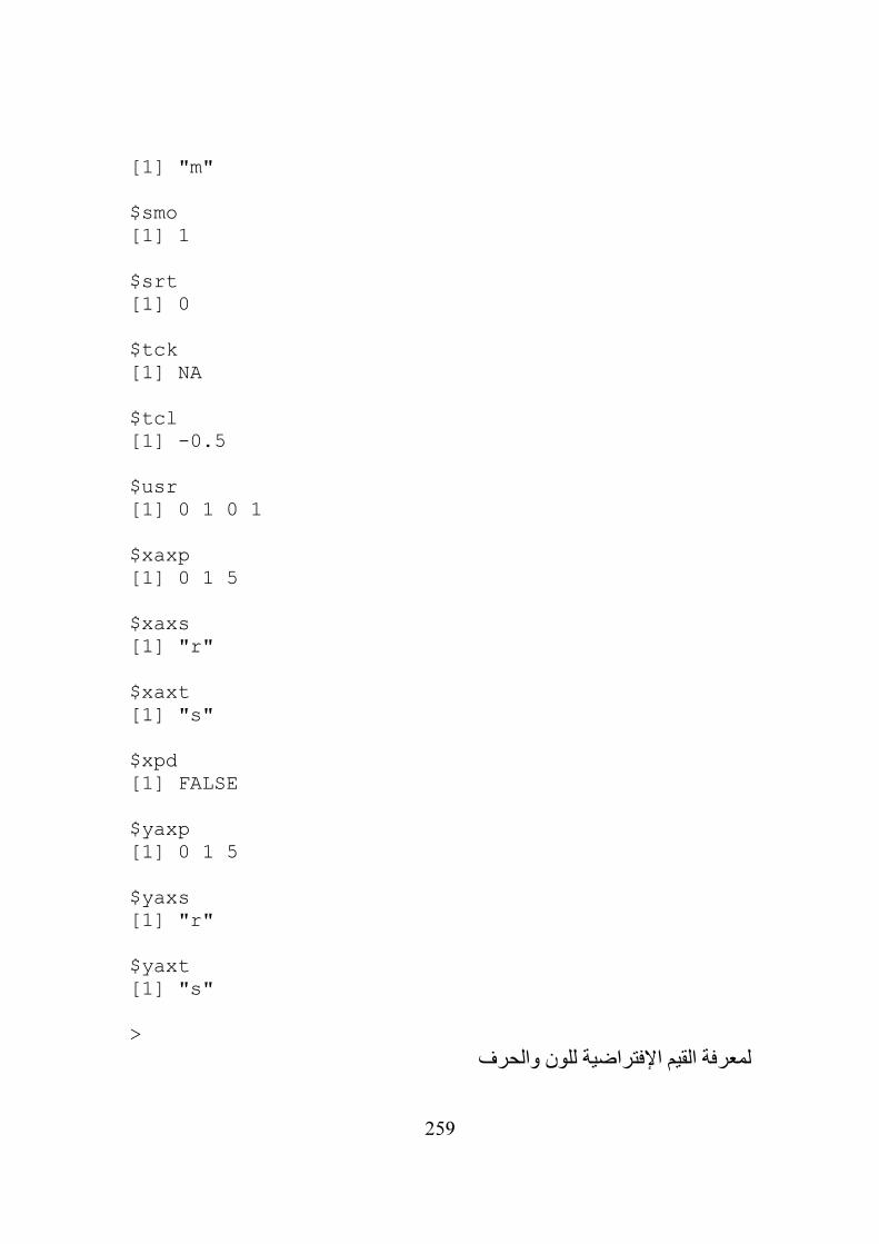
259
[1] "m" $smo [1] 1 $srt [1] 0 $tck [1] NA $tcl [1] -0.5 $usr [1] 0 1 0 1 $xaxp [1] 0 1 5 $xaxs [1] "r" $xaxt [1] "s" $xpd [1] FALSE $yaxp [1] 0 1 5 $yaxs [1] "r" $yaxt [1] "s" >
لمعرفة القيم اإلفتراضية للون والحرف

260
> par(c("pch", "col"))
$pch [1] 1 $col [1] "black" >
*لتغيير الحرف اإلفتراضي إلى > par(pch="*")
الرسومات التفاعلية:
والتي (…)identifyعدد من إمكانيات الرسم التفاعلي وأحد هذه هو الدالة Rتمتلك سوف (…)identifyتمكن من تأشير نقاط مهمة في الرسم. الحظ بعد إدخال الدالة
إختيار النقاط مستخدما الفارة وتوقف العملية ينتظر البرنامج حتى يستطيع المستخدم بإستخدام الزر األيمن للفارة
> plot(exam1,exam2)
> identify(exam1,exam2)
[1] 17 45 55 >
261
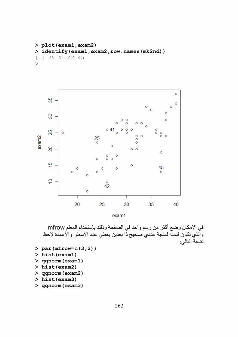
262
> plot(exam1,exam2)
> identify(exam1,exam2,row.names(mk2nd))
[1] 25 41 42 45 >
mfrowوذلك بإستخدام المعلم في اإلمكان وضع أكثر من رسم واحد في الصفحة
والذي تكون قيمته لمتجة عددي صحيح ذا بعدين يعطي عدد األسطر واألعمدة الحظ نتيجة التالي:
> par(mfrow=c(3,2))
> hist(exam1)
> qqnorm(exam1)
> hist(exam2)
> qqnorm(exam2)
> hist(exam3)
> qqnorm(exam3)
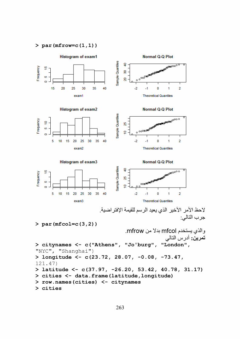
263
> par(mfrow=c(1,1))
األخير الذي يعيد الرسم للقيمة اإلفتراضية.الحظ األمر جرب التالي:
> par(mfcol=c(3,2))
.mfrowبدال من mfcolوالذي يستخدم أدرس التالي تمرين:
> citynames <- c("Athens", "Jo'burg", "London", "NYC", "Shanghai") > longitude <- c(23.72, 28.07, -0.08, -73.47, 121.47) > latitude <- c(37.97, -26.20, 53.42, 40.78, 31.17)
> cities <- data.frame(latitude,longitude)
> row.names(cities) <- citynames
> cities
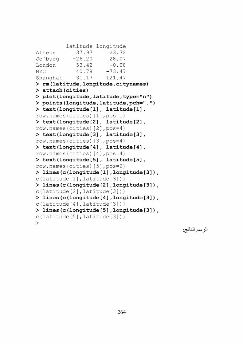
264
latitude longitude Athens 37.97 23.72 Jo'burg -26.20 28.07 London 53.42 -0.08 NYC 40.78 -73.47 Shanghai 31.17 121.47 > rm(latitude,longitude,citynames)
> attach(cities)
> plot(longitude,latitude,type="n")
> points(longitude,latitude,pch=".")
> text(longitude[1], latitude[1], row.names(cities)[1],pos=1) > text(longitude[2], latitude[2], row.names(cities)[2],pos=4) > text(longitude[3], latitude[3], row.names(cities)[3],pos=4) > text(longitude[4], latitude[4], row.names(cities)[4],pos=4) > text(longitude[5], latitude[5], row.names(cities)[5],pos=2) > lines(c(longitude[1],longitude[3]), c(latitude[1],latitude[3])) > lines(c(longitude[2],longitude[3]), c(latitude[2],latitude[3])) > lines(c(longitude[4],longitude[3]), c(latitude[4],latitude[3])) > lines(c(longitude[5],longitude[3]), c(latitude[5],latitude[3])) >
الرسم الناتج:
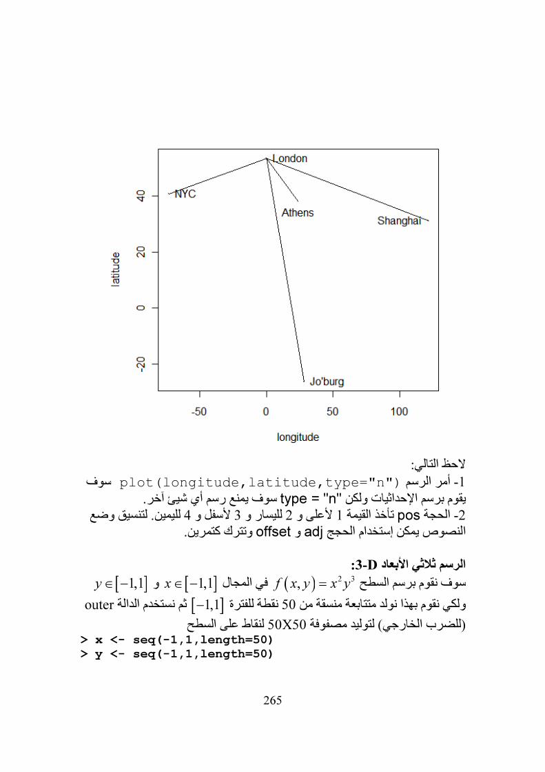
265
لي:الحظ التا
سوف plot(longitude,latitude,type="n")أمر الرسم -1 سوف يمنع رسم أي شيئ آخر. "type = "nيقوم برسم اإلحداثيات ولكن
لليمين. لتنسيق وضع 4ألسفل و 3لليسار و 2ألعلى و 1تأخذ القيمة posالحجة -2 وتترك كتمرين. offsetو adjالنصوص يمكن إستخدام الحجج
:D-3ثي األبعاد الرسم ثال
)سوف نقوم برسم السطح ) 2 3,f x y x y= في المجال[ ]1,1x∈ ]و − ]1,1y∈ −
]نقطة للفترة 50ولكي نقوم بهذا نولد متتابعة منسقة من outerثم نستخدم الدالة −1,1[
لنقاط على السطح 50X50يد مصفوفة (للضرب الخارجي) لتول> x <- seq(-1,1,length=50)
> y <- seq(-1,1,length=50)
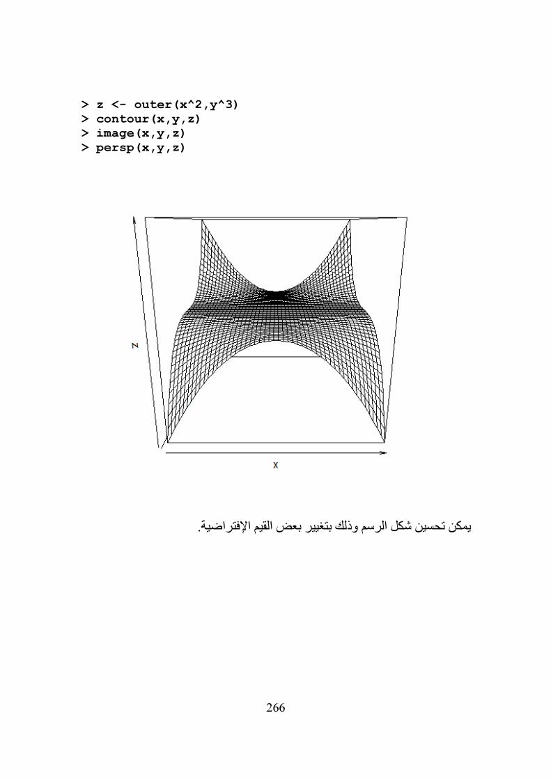
266
> z <- outer(x^2,y^3)
> contour(x,y,z)
> image(x,y,z)
> persp(x,y,z)
يمكن تحسين شكل الرسم وذلك بتغيير بعض القيم اإلفتراضية.

267
: essentials Rأساسيات
يقوم البرنامج بحفظ األوامر المدخلة من لوحة المفاتيح في R في أي جلسة من جلساتوقد ↓أو ↑ويمكن إستعادة هذه األوامر بأحد المفاتيح bufferمنطقة من الذاكرة
التاريخ يكون من المفيد تخزين هذة األوامر لإلستخدام في جلسة أخرى لهذا نحفظ هذا باألمر:
> savehistory("filename.Rhistory")
وتستعاد باألمر:> loadhistory("filename.Rhistory")
أما إذا شئنا إجراء هذه ↓أو ↑بعد إستعادة األوامر يمكن إستخدامها بأحد المفاتيح األوامر نستخدم األمر:
> source("filename ", echo=TRUE)
The search pathمسار البحث
بالبحث عن الشيئ التابع للمعرف. أول مكان تبحث فيه Rعند إمرار معرف لدالة تقوم
R هو فضاء العمل ( والذي يعرف أيضا باإلسم البيئة الشاملةglobal environment بالبحث Rشيئ في فضاء العمل سيقوم ) إذا لم يوجد هذا ال GlobalEnv.ويرمز له
في أي قائمة مضافة (بما فيها أطر البيانات) والحزم المحملة بواسطة المستخدم والحزم الحقيقي حيث أنها تضع قائمة في (…)attachالمحملة ذاتيا ومن هنا تتضح عمل
تعطي مسار ()searchتزيلها من المسار. الدالة (…)detachمسار البحث و وإعطاء إسم أي بيئة أو موقعها لدالة األشياء سوف يقوم بسرد األشياء في تلك البحث البيئة
> search()
> objects(package:MASS)
> objects(4)
:packages Rحزم
إلعطائها Rوهي عبارة عن ملفات تحوي برامج إضافية متخصصة تضاف إلى
. وفي مقدورنا سرد قائمة Rساس مقدرات لحل مجال أكبر من المشاكل التتوفر في أ. (…)libraryبالحزم المتوفرة وكذلك تحميل هذه الحزم وتجديدها بإستخدام األمر
األمر التالي يسرد كل الحزم المتوفرة> library() Packages in library 'C:/PROGRA~1/R/R-28~1.1/library':

268
base The R Base Package boot Bootstrap R (S-Plus) Functions (Canty) class Functions for Classification cluster Cluster Analysis Extended Rousseeuw et al. codetools Code Analysis Tools for R datasets The R Datasets Package foreign Read Data Stored by Minitab, S, SAS, SPSS, Stata, Systat, dBase, ... graphics The R Graphics Package grDevices The R Graphics Devices and Support for Colours and Fonts grid The Grid Graphics Package KernSmooth Functions for kernel smoothing for Wand & Jones (1995) lattice Lattice Graphics MASS Main Package of Venables and Ripley's MASS methods Formal Methods and Classes mgcv GAMs with GCV/AIC/REML smoothness estimation and GAMMs by PQL nlme Linear and Nonlinear Mixed Effects Models nnet Feed-forward Neural Networks and Multinomial Log-Linear Models R.methodsS3 Utility function for defining S3 methods R.oo R object-oriented programming with or without references rpart Recursive Partitioning Sim101 Sim 101 Package for WSC 2008 spatial Functions for Kriging and Point Pattern Analysis splines Regression Spline Functions and Classes stats The R Stats Package stats4 Statistical Functions using S4 Classes survival Survival analysis, including penalised likelihood. tcltk Tcl/Tk Interface tools Tools for Package Development utils The R Utils Package
MASSاألمرالتالي يحمل الحزمة > library(MASS)
ونستطيع مشاهدة محتواه> library(help=MASS) Information on package 'MASS' Description:

269
Bundle: VR Priority: recommended Contains: MASS class nnet spatial Version: 7.2-45 Date: 2008-12-07 Depends: R (>= 2.4.0), grDevices, graphics, stats, utils Suggests: lattice, nlme, survival Author: S original by Venables & Ripley. R port by Brian Ripley <[email protected]>, following earlier work by Kurt Hornik and Albrecht Gebhardt. Maintainer: Brian Ripley <[email protected]> BundleDescription: Functions and datasets to support Venables and Ripley, 'Modern Applied Statistics with S' (4th edition). License: GPL-2 | GPL-3 URL: http://www.stats.ox.ac.uk/pub/MASS4/ Packaged: Tue Dec 9 11:11:17 2008; ripley Package: MASS Description: The main library and the datasets Title: Main Package of Venables and Ripley's MASS LazyLoad: yes LazyData: yes Built: R 2.8.1; i386-pc-mingw32; 2008-12-22 09:22:56; windows Index: Functions: ========= Null Null Spaces of Matrices addterm Try All One-Term Additions to a Model anova.negbin Likelihood Ratio Tests for Negative Binomial GLMs area Adaptive Numerical Integration bandwidth.nrd Bandwidth for density() via Normal Reference Distribution bcv Biased Cross-Validation for Bandwidth Selection boxcox Box-Cox Transformations for Linear Models con2tr Convert Lists to Data Frames for use by Trellis confint-MASS Confidence Intervals for Model Parameters contr.sdif Successive Differences contrast coding corresp Simple Correspondence Analysis cov.rob Resistant Estimation of Multivariate Location and Scatter

270
cov.trob Covariance Estimation for Multivariate t Distribution denumerate Transform an Allowable Formula for 'loglm' into one for 'terms' dose.p Predict Doses for Binomial Assay model dropterm Try All One-Term Deletions from a Model eqscplot Plots with Geometrically Equal Scales fitdistr Maximum-likelihood Fitting of Univariate Distributions fractions Rational Approximation gamma.dispersion Calculate the MLE of the Gamma Dispersion Parameter in a GLM Fit gamma.shape Estimate the Shape Parameter of the Gamma Distribution in a GLM Fit ginv Generalized Inverse of a Matrix glm.convert Change a Negative Binomial fit to a GLM fit glm.nb Fit a Negative Binomial Generalized Linear Model glmmPQL Fit Generalized Linear Mixed Models via PQL hist.scott Plot a Histogram with Automatic Bin Width Selection huber Huber M-estimator of Location with MAD Scale hubers Huber Proposal 2 Robust Estimator of Location and/or Scale isoMDS Kruskal's Non-metric Multidimensional Scaling kde2d Two-Dimensional Kernel Density Estimation lda Linear Discriminant Analysis ldahist Histograms or Density Plots of Multiple Groups lm.gls Fit Linear Models by Generalized Least Squares lm.ridge Ridge Regression loglm Fit Log-Linear Models by Iterative Proportional Scaling logtrans Estimate log Transformation Parameter lqs Resistant Regression mca Multiple Correspondence Analysis mvrnorm Simulate from a Multivariate Normal Distribution negative.binomial Family function for Negative Binomial GLMs newcomb Newcomb's Measurements of the Passage Time of Light

271
pairs.lda Produce Pairwise Scatterplots from an 'lda' Fit parcoord Parallel Coordinates Plot plot.lda Plot Method for Class 'lda' plot.mca Plot Method for Objects of Class 'mca' polr Proportional Odds Logistic Regression predict.lda Classify Multivariate Observations by Linear Discrimination predict.lqs Predict from an lqs Fit predict.mca Predict Method for Class 'mca' predict.qda Classify from Quadratic Discriminant Analysis qda Quadratic Discriminant Analysis rational Rational Approximation renumerate Convert a Formula Transformed by 'denumerate' rlm Robust Fitting of Linear Models rms.curv Relative Curvature Measures for Non-Linear Regression rnegbin Simulate Negative Binomial Variates sammon Sammon's Non-Linear Mapping stdres Extract Standardized Residuals from a Linear Model stepAIC Choose a model by AIC in a Stepwise Algorithm studres Extract Studentized Residuals from a Linear Model summary.loglm Summary Method Function for Objects of Class 'loglm' summary.negbin Summary Method Function for Objects of Class 'negbin' summary.rlm Summary Method for Robust Linear Models synth.tr Synthetic Classification Problem theta.md Estimate theta of the Negative Binomial by Deviance theta.ml Estimate theta of the Negative Binomial by Maximum Likelihood theta.mm Estimate theta of the Negative Binomial by Moments truehist Plot a Histogram ucv Unbiased Cross-Validation for Bandwidth Selection width.SJ Bandwidth Selection by Pilot Estimation of Derivatives write.matrix Write a Matrix or Data Frame Datasets: ========

272
Aids2 Australian AIDS Survival Data Animals Brain and Body Weights for 28 Species Belgian-phones Belgium Phone Calls 1950-1973 Boston Housing Values in Suburbs of Boston Cars93 Data from 93 Cars on Sale in the USA in 1993 Cushings Diagnostic Tests on Patients with Cushing's Syndrome DDT DDT in Kale GAGurine Level of GAG in Urine of Children Insurance Numbers of Car Insurance claims Melanoma Survival from Malignant Melanoma OME Tests of Auditory Perception in Children with OME Pima.tr Diabetes in Pima Indian Women Rabbit Blood Pressure in Rabbits Rubber Accelerated Testing of Tyre Rubber SP500 Returns of the Standard and Poors 500 Sitka Growth Curves for Sitka Spruce Trees in 1988 Sitka89 Growth Curves for Sitka Spruce Trees in 1989 Skye AFM Compositions of Aphyric Skye Lavas Traffic Effect of Swedish Speed Limits on Accidents UScereal Nutritional and Marketing Information on US Cereals UScrime The Effect of Punishment Regimes on Crime Rates VA Veteran's Administration Lung Cancer Trial abbey Determinations of Nickel Content accdeaths Accidental Deaths in the US 1973-1978 anorexia Anorexia Data on Weight Change bacteria Presence of Bacteria after Drug Treatments beav1 Body Temperature Series of Beaver 1 beav2 Body Temperature Series of Beaver 2 biopsy Biopsy Data on Breast Cancer Patients birthwt Risk Factors Associated with Low Infant Birth Weight cabbages Data from a cabbage field trial caith Colours of Eyes and Hair of People in Caithness cats Anatomical Data from Domestic Cats cement Heat Evolved by Setting Cements chem Copper in Wholemeal Flour coop Co-operative Trial in Analytical Chemistry cpus Performance of Computer CPUs crabs Morphological Measurements on Leptograpsus Crabs

273
drivers Deaths of Car Drivers in Great Britain 1969-84 eagles Foraging Ecology of Bald Eagles epil Seizure Counts for Epileptics farms Ecological Factors in Farm Management fgl Measurements of Forensic Glass Fragments forbes Forbes' Data on Boiling Points in the Alps galaxies Velocities for 82 Galaxies gehan Remission Times of Leukaemia Patients genotype Rat Genotype Data geyser Old Faithful Geyser Data gilgais Line Transect of Soil in Gilgai Territory hills Record Times in Scottish Hill Races housing Frequency Table from a Copenhagen Housing Conditions Survey immer Yields from a Barley Field Trial leuk Survival Times and White Blood Counts for Leukaemia Patients mammals Brain and Body Weights for 62 Species of Land Mammals mcycle Data from a Simulated Motorcycle Accident menarche Age of Menarche data michelson Michelson's Speed of Light Data minn38 Minnesota High School Graduates of 1938 motors Accelerated Life Testing of Motorettes muscle Effect of Calcium Chloride on Muscle Contraction in Rat Hearts nlschools Eighth-Grade Pupils in the Netherlands npk Classical N, P, K Factorial Experiment npr1 US Naval Petroleum Reserve No. 1 data oats Data from an Oats Field Trial painters The Painter's Data of de Piles petrol N. L. Prater's Petrol Refinery Data quine Absenteeism from School in Rural New South Wales road Road Accident Deaths in US States rotifer Numbers of Rotifers by Fluid Density ships Ships Damage Data shoes Shoe wear data of Box, Hunter and Hunter shrimp Percentage of Shrimp in Shrimp Cocktail shuttle Space Shuttle Autolander Problem snails Snail Mortality Data steam The Saturated Steam Pressure Data stormer The Stormer Viscometer Data survey Student Survey Data topo Spatial Topographic Data waders Counts of Waders at 15 Sites in South Africa whiteside House Insulation: Whiteside's Data

274
wtloss Weight Loss Data from an Obese Patient
ة باألمر يالحظ أن بعض الحزم تحوي مجاميع بيانات ونستطيع معرفة البيانات الموجودdata() والذي يسرد مجاميع البيانات للحزم المحملة حاليا
> data() Data sets in package ‘datasets’: AirPassengers Monthly Airline Passenger Numbers 1949-1960 BJsales Sales Data with Leading Indicator BJsales.lead (BJsales) Sales Data with Leading Indicator BOD Biochemical Oxygen Demand CO2 Carbon Dioxide uptake in grass plants ChickWeight Weight versus age of chicks on different diets DNase Elisa assay of DNase EuStockMarkets Daily Closing Prices of Major European Stock Indices, 1991-1998 Formaldehyde Determination of Formaldehyde HairEyeColor Hair and Eye Color of Statistics Students Harman23.cor Harman Example 2.3 Harman74.cor Harman Example 7.4 Indometh Pharmacokinetics of Indomethicin InsectSprays Effectiveness of Insect Sprays JohnsonJohnson Quarterly Earnings per Johnson & Johnson Share LakeHuron Level of Lake Huron 1875-1972 LifeCycleSavings Intercountry Life-Cycle Savings Data Loblolly Growth of Loblolly pine trees Nile Flow of the River Nile Orange Growth of Orange Trees OrchardSprays Potency of Orchard Sprays PlantGrowth Results from an Experiment on Plant Growth Puromycin Reaction velocity of an enzymatic reaction Seatbelts Road Casualties in Great Britain 1969-84 Theoph Pharmacokinetics of theophylline Titanic Survival of passengers on the Titanic ToothGrowth The Effect of Vitamin C on Tooth Growth in Guinea Pigs UCBAdmissions Student Admissions at UC Berkeley UKDriverDeaths Road Casualties in Great Britain 1969-84 UKgas UK Quarterly Gas Consumption USAccDeaths Accidental Deaths in the US 1973-1978 USArrests Violent Crime Rates by US State USJudgeRatings Lawyers' Ratings of State Judges in the US Superior Court USPersonalExpenditure Personal Expenditure Data VADeaths Death Rates in Virginia (1940)

275
WWWusage Internet Usage per Minute WorldPhones The World's Telephones ability.cov Ability and Intelligence Tests airmiles Passenger Miles on Commercial US Airlines, 1937-1960 airquality New York Air Quality Measurements anscombe Anscombe's Quartet of "Identical" Simple Linear Regressions attenu The Joyner-Boore Attenuation Data attitude The Chatterjee-Price Attitude Data austres Quarterly Time Series of the Number of Australian Residents beaver1 (beavers) Body Temperature Series of Two Beavers beaver2 (beavers) Body Temperature Series of Two Beavers cars Speed and Stopping Distances of Cars chickwts Chicken Weights by Feed Type co2 Mauna Loa Atmospheric CO2 Concentration crimtab Student's 3000 Criminals Data discoveries Yearly Numbers of Important Discoveries esoph Smoking, Alcohol and (O)esophageal Cancer euro Conversion Rates of Euro Currencies euro.cross (euro) Conversion Rates of Euro Currencies eurodist Distances Between European Cities faithful Old Faithful Geyser Data fdeaths (UKLungDeaths) Monthly Deaths from Lung Diseases in the UK freeny Freeny's Revenue Data freeny.x (freeny) Freeny's Revenue Data freeny.y (freeny) Freeny's Revenue Data infert Infertility after Spontaneous and Induced Abortion iris Edgar Anderson's Iris Data iris3 Edgar Anderson's Iris Data islands Areas of the World's Major Landmasses ldeaths (UKLungDeaths) Monthly Deaths from Lung Diseases in the UK lh Luteinizing Hormone in Blood Samples longley Longley's Economic Regression Data lynx Annual Canadian Lynx trappings 1821-1934 mdeaths (UKLungDeaths) Monthly Deaths from Lung Diseases in the UK morley Michaelson-Morley Speed of Light Data mtcars Motor Trend Car Road Tests nhtemp Average Yearly Temperatures in New Haven nottem Average Monthly Temperatures at Nottingham, 1920-1939 occupationalStatus Occupational Status of Fathers and their Sons precip Annual Precipitation in US Cities presidents Quarterly Approval Ratings of US Presidents pressure Vapor Pressure of Mercury as a Function of Temperature

276
quakes Locations of Earthquakes off Fiji randu Random Numbers from Congruential Generator RANDU rivers Lengths of Major North American Rivers rock Measurements on Petroleum Rock Samples sleep Student's Sleep Data stack.loss (stackloss) Brownlee's Stack Loss Plant Data stack.x (stackloss) Brownlee's Stack Loss Plant Data stackloss Brownlee's Stack Loss Plant Data state.abb (state) US State Facts and Figures state.area (state) US State Facts and Figures state.center (state) US State Facts and Figures state.division (state) US State Facts and Figures state.name (state) US State Facts and Figures state.region (state) US State Facts and Figures state.x77 (state) US State Facts and Figures sunspot.month Monthly Sunspot Data, 1749-1997 sunspot.year Yearly Sunspot Data, 1700-1988 sunspots Monthly Sunspot Numbers, 1749-1983 swiss Swiss Fertility and Socioeconomic Indicators (1888) Data treering Yearly Treering Data, -6000-1979 trees Girth, Height and Volume for Black Cherry Trees uspop Populations Recorded by the US Census volcano Topographic Information on Auckland's Maunga Whau Volcano warpbreaks The Number of Breaks in Yarn during Weaving women Average Heights and Weights for American Women Data sets in package ‘MASS’: Aids2 Australian AIDS Survival Data Animals Brain and Body Weights for 28 Species Boston Housing Values in Suburbs of Boston Cars93 Data from 93 Cars on Sale in the USA in 1993 Cushings Diagnostic Tests on Patients with Cushing's Syndrome DDT DDT in Kale GAGurine Level of GAG in Urine of Children Insurance Numbers of Car Insurance claims Melanoma Survival from Malignant Melanoma OME Tests of Auditory Perception in Children with OME

277
Pima.te Diabetes in Pima Indian Women Pima.tr Diabetes in Pima Indian Women Pima.tr2 Diabetes in Pima Indian Women Rabbit Blood Pressure in Rabbits Rubber Accelerated Testing of Tyre Rubber SP500 Returns of the Standard and Poors 500 Sitka Growth Curves for Sitka Spruce Trees in 1988 Sitka89 Growth Curves for Sitka Spruce Trees in 1989 Skye AFM Compositions of Aphyric Skye Lavas Traffic Effect of Swedish Speed Limits on Accidents UScereal Nutritional and Marketing Information on US Cereals UScrime The Effect of Punishment Regimes on Crime Rates VA Veteran's Administration Lung Cancer Trial abbey Determinations of Nickel Content accdeaths Accidental Deaths in the US 1973-1978 anorexia Anorexia Data on Weight Change bacteria Presence of Bacteria after Drug Treatments beav1 Body Temperature Series of Beaver 1 beav2 Body Temperature Series of Beaver 2 biopsy Biopsy Data on Breast Cancer Patients birthwt Risk Factors Associated with Low Infant Birth Weight cabbages Data from a cabbage field trial caith Colours of Eyes and Hair of People in Caithness cats Anatomical Data from Domestic Cats cement Heat Evolved by Setting Cements chem Copper in Wholemeal Flour coop Co-operative Trial in Analytical Chemistry cpus Performance of Computer CPUs crabs Morphological Measurements on Leptograpsus Crabs deaths Monthly Deaths from Lung Diseases in the UK drivers Deaths of Car Drivers in Great Britain 1969-84 eagles Foraging Ecology of Bald Eagles epil Seizure Counts for Epileptics farms Ecological Factors in Farm Management fgl Measurements of Forensic Glass Fragments forbes Forbes' Data on Boiling Points in the Alps galaxies Velocities for 82 Galaxies gehan Remission Times of Leukaemia Patients genotype Rat Genotype Data geyser Old Faithful Geyser Data gilgais Line Transect of Soil in Gilgai Territory hills Record Times in Scottish Hill Races housing Frequency Table from a Copenhagen Housing Conditions Survey

278
immer Yields from a Barley Field Trial leuk Survival Times and White Blood Counts for Leukaemia Patients mammals Brain and Body Weights for 62 Species of Land Mammals mcycle Data from a Simulated Motorcycle Accident menarche Age of Menarche in Warsaw michelson Michelson's Speed of Light Data minn38 Minnesota High School Graduates of 1938 motors Accelerated Life Testing of Motorettes muscle Effect of Calcium Chloride on Muscle Contraction in Rat Hearts newcomb Newcomb's Measurements of the Passage Time of Light nlschools Eighth-Grade Pupils in the Netherlands npk Classical N, P, K Factorial Experiment npr1 US Naval Petroleum Reserve No. 1 data oats Data from an Oats Field Trial painters The Painter's Data of de Piles petrol N. L. Prater's Petrol Refinery Data phones Belgium Phone Calls 1950-1973 quine Absenteeism from School in Rural New South Wales road Road Accident Deaths in US States rotifer Numbers of Rotifers by Fluid Density ships Ships Damage Data shoes Shoe wear data of Box, Hunter and Hunter shrimp Percentage of Shrimp in Shrimp Cocktail shuttle Space Shuttle Autolander Problem snails Snail Mortality Data steam The Saturated Steam Pressure Data stormer The Stormer Viscometer Data survey Student Survey Data synth.te Synthetic Classification Problem synth.tr Synthetic Classification Problem topo Spatial Topographic Data waders Counts of Waders at 15 Sites in South Africa whiteside House Insulation: Whiteside's Data wtloss Weight Loss Data from an Obese Patient Use ‘data(package = .packages(all.available = TRUE))’ to list the data sets in all *available* packages.
وإضافة مجموعة بيانات إلى حزمة> data(mydata, package=MASS)
الحوار التالي لتحميل حزمة
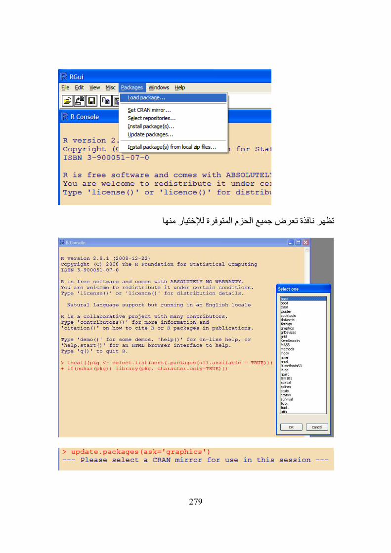
279
تظهر نافذة تعرض جميع الحزم المتوفرة لإلختيار منها
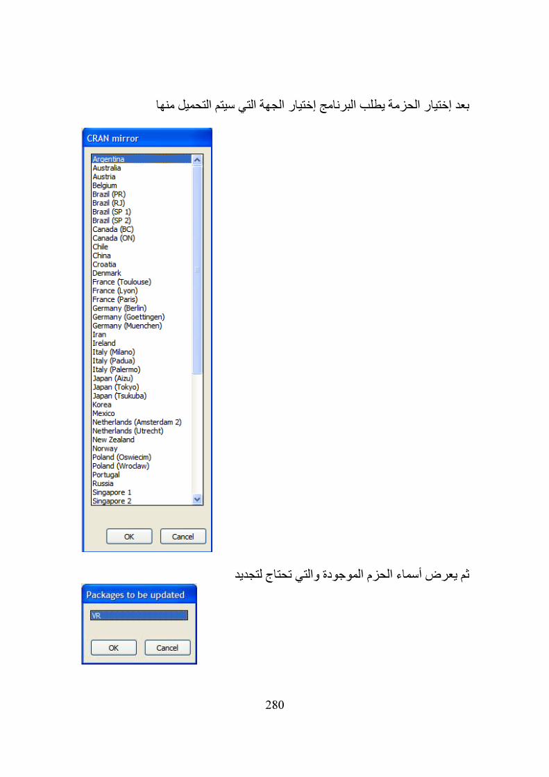
280
بعد إختيار الحزمة يطلب البرنامج إختيار الجهة التي سيتم التحميل منها
ثم يعرض أسماء الحزم الموجودة والتي تحتاج لتجديد
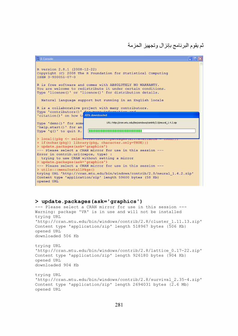
281
ثم يقوم البرنامج بإنزال وتجهيز الحزمة
> update.packages(ask='graphics') --- Please select a CRAN mirror for use in this session --- Warning: package 'VR' is in use and will not be installed trying URL 'http://cran.mtu.edu/bin/windows/contrib/2.8/cluster_1.11.13.zip' Content type 'application/zip' length 518967 bytes (506 Kb) opened URL downloaded 506 Kb trying URL 'http://cran.mtu.edu/bin/windows/contrib/2.8/lattice_0.17-22.zip' Content type 'application/zip' length 926180 bytes (904 Kb) opened URL downloaded 904 Kb trying URL 'http://cran.mtu.edu/bin/windows/contrib/2.8/survival_2.35-4.zip' Content type 'application/zip' length 2694031 bytes (2.6 Mb) opened URL

282
downloaded 2.6 Mb package 'cluster' successfully unpacked and MD5 sums checked package 'lattice' successfully unpacked and MD5 sums checked Warning: cannot remove prior installation of package 'lattice' package 'survival' successfully unpacked and MD5 sums checked The downloaded packages are in C:\Documents and Settings\amb\Local Settings\Temp\RtmptdGcgZ\downloaded_packages updating HTML package descriptions >
> utils:::menuInstallPkgs() trying URL 'http://cran.mtu.edu/bin/windows/contrib/2.8/neural_1.4.2.zip' Content type 'application/zip' length 59600 bytes (58 Kb) opened URL downloaded 58 Kb package 'neural' successfully unpacked and MD5 sums checked The downloaded packages are in C:\Documents and Settings\amb\Local Settings\Temp\Rtmp1dLn2q\downloaded_packages updating HTML package descriptions
> library(neural)
> library(help = neural) >
Information on package 'neural' Description: Package: neural Version: 1.4.2 Title: Neural Networks Author: Ádám Nagy Maintainer: Ádám Nagy <[email protected]> Description: RBF and MLP neural networks with graphical user interface License: GPL version 2 or later Built: R 2.8.1; ; 2008-12-14 01:45:38; windows Index: mlp MLP neural network recalling method
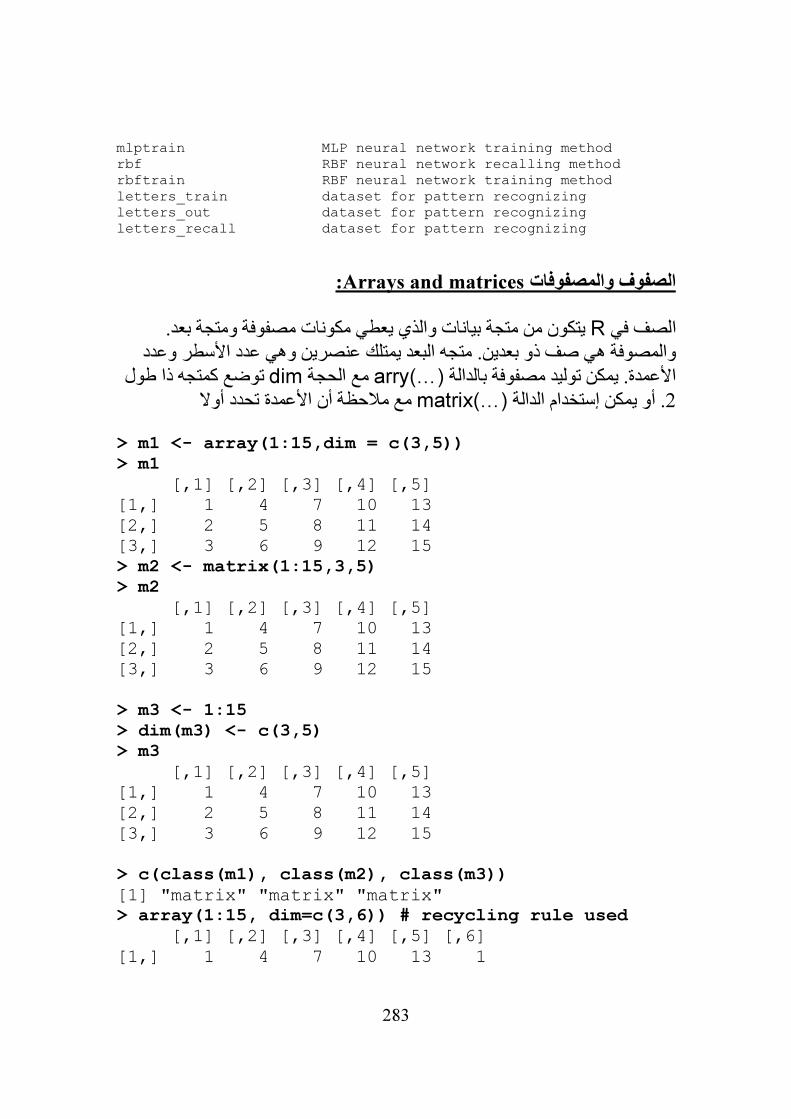
283
mlptrain MLP neural network training method rbf RBF neural network recalling method rbftrain RBF neural network training method letters_train dataset for pattern recognizing letters_out dataset for pattern recognizing letters_recall dataset for pattern recognizing
:Arrays and matricesالصفوف والمصفوفات
يتكون من متجة بيانات والذي يعطي مكونات مصفوفة ومتجة بعد. Rالصف في والمصوفة هي صف ذو بعدين. متجه البعد يمتلك عنصرين وهي عدد األسطر وعدد
كمتجه ذا طول توضع dimمع الحجة (…)arryاألعمدة. يمكن توليد مصفوفة بالدالة مع مالحظة أن األعمدة تحدد أوال (…)matrix. أو يمكن إستخدام الدالة 2
> m1 <- array(1:15,dim = c(3,5))
> m1
[,1] [,2] [,3] [,4] [,5] [1,] 1 4 7 10 13 [2,] 2 5 8 11 14 [3,] 3 6 9 12 15 > m2 <- matrix(1:15,3,5)
> m2
[,1] [,2] [,3] [,4] [,5] [1,] 1 4 7 10 13 [2,] 2 5 8 11 14 [3,] 3 6 9 12 15
> m3 <- 1:15
> dim(m3) <- c(3,5)
> m3
[,1] [,2] [,3] [,4] [,5] [1,] 1 4 7 10 13 [2,] 2 5 8 11 14 [3,] 3 6 9 12 15
> c(class(m1), class(m2), class(m3))
[1] "matrix" "matrix" "matrix" > array(1:15, dim=c(3,6)) # recycling rule used
[,1] [,2] [,3] [,4] [,5] [,6] [1,] 1 4 7 10 13 1
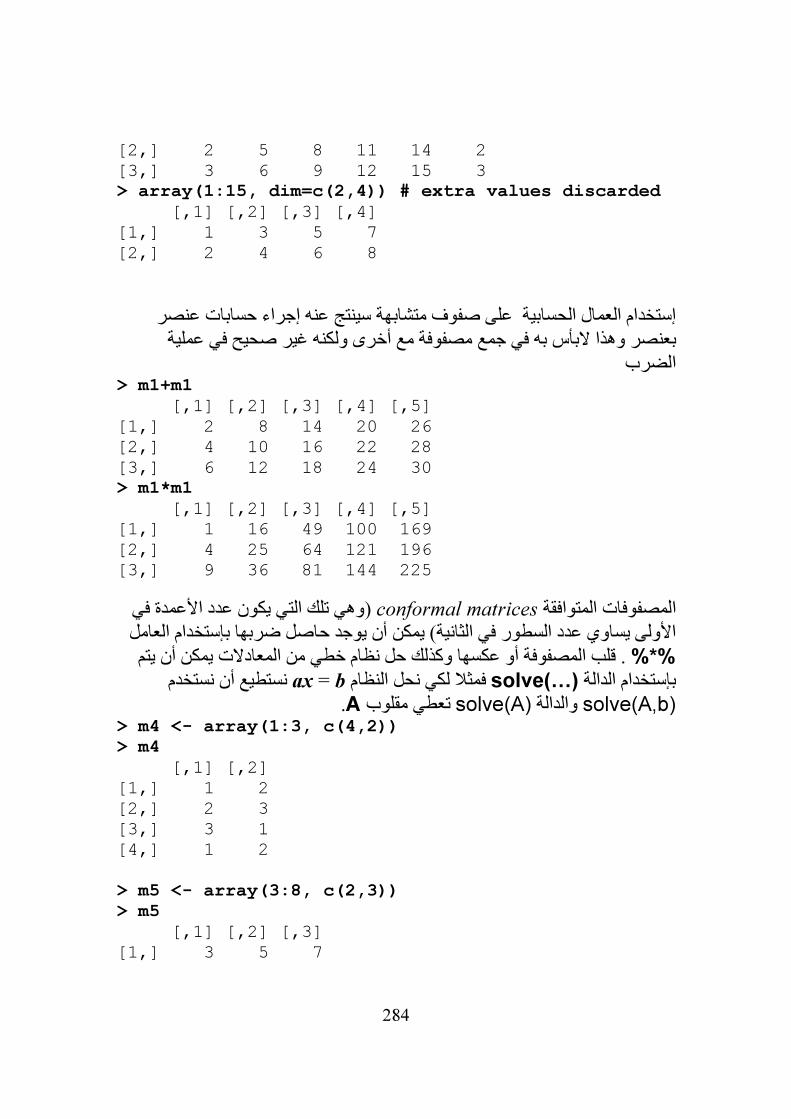
284
[2,] 2 5 8 11 14 2 [3,] 3 6 9 12 15 3 > array(1:15, dim=c(2,4)) # extra values discarded
[,1] [,2] [,3] [,4] [1,] 1 3 5 7 [2,] 2 4 6 8
إستخدام العمال الحسابية على صفوف متشابهة سينتج عنه إجراء حسابات عنصر ي جمع مصفوفة مع أخرى ولكنه غير صحيح في عملية بعنصر وهذا البأس به ف
الضرب > m1+m1
[,1] [,2] [,3] [,4] [,5] [1,] 2 8 14 20 26 [2,] 4 10 16 22 28 [3,] 6 12 18 24 30 > m1*m1
[,1] [,2] [,3] [,4] [,5] [1,] 1 16 49 100 169 [2,] 4 25 64 121 196 [3,] 9 36 81 144 225
(وهي تلك التي يكون عدد األعمدة في conformal matricesالمصفوفات المتوافقة األولى يساوي عدد السطور في الثانية) يمكن أن يوجد حاصل ضربها بإستخدام العامل
دالت يمكن أن يتم . قلب المصفوفة أو عكسها وكذلك حل نظام خطي من المعا %*%نستطيع أن نستخدم ax = bفمثال لكي نحل النظام (…)solveبإستخدام الدالة solve(A,b) والدالةsolve(A) تعطي مقلوبA.
> m4 <- array(1:3, c(4,2))
> m4
[,1] [,2] [1,] 1 2 [2,] 2 3 [3,] 3 1 [4,] 1 2
> m5 <- array(3:8, c(2,3))
> m5
[,1] [,2] [,3] [1,] 3 5 7
285
[2,] 4 6 8
> m4 %*% m5
[,1] [,2] [,3] [1,] 11 17 23 [2,] 18 28 38 [3,] 13 21 29 [4,] 11 17 23
> m6 <- array(c(1,3,2,1),c(2,2))
> m6
[,1] [,2] [1,] 1 2 [2,] 3 1 > v1 <- array(c(1,0), c(2,1))
> v1
[,1] [1,] 1 [2,] 0 > solve(m6,v1)
[,1] [1,] -0.2 [2,] 0.6
> solve(m6) # inverts m6
[,1] [,2] [1,] -0.2 0.4 [2,] 0.6 -0.2
> solve(m6) %*% v1 # does the same as solve(m6,v1)
[,1] [1,] -0.2 [2,] 0.6
لصفين هو مصفوفة تتولد من كل تراكيب ممكنة outer productالضرب الخارجي
هي المتجهين والحجة الثالثة (…)outerلعناصرهم. الحجتين األولى والثانية في الدلة هي العملية المطلوب القيام بها (القيمة اإلفتراضية هي الضرب) وهنا نحن نبسط األمر
رب الخارجي يعمل على متجهات بأبعاد عامة (وليس متجهات وحسب) والمثال ألن الضوالتي عناصرها تأتي من 2X2التالي يوضح ذلك. المطلوب توليد دالة الكتلة للمصفوفة
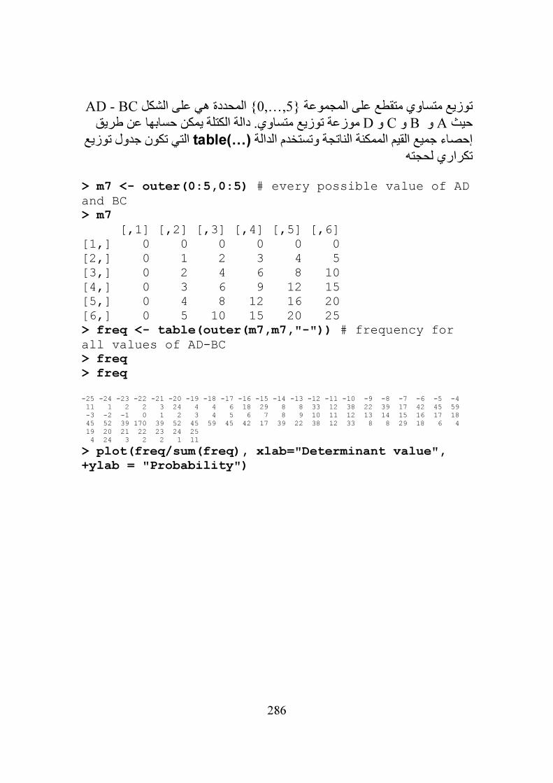
286
AD - BCالمحددة هي على الشكل {5,…,0}توزيع متساوي متقطع على المجموعة الكتلة يمكن حسابها عن طريق موزعة توزيع متساوي. دالة Dو Cو Bو Aحيث
التي تكون جدول توزيع (…)tableإحصاء جميع القيم الممكنة الناتجة وتستخدم الدالة تكراري لحجته
> m7 <- outer(0:5,0:5) # every possible value of AD and BC > m7
[,1] [,2] [,3] [,4] [,5] [,6] [1,] 0 0 0 0 0 0 [2,] 0 1 2 3 4 5 [3,] 0 2 4 6 8 10 [4,] 0 3 6 9 12 15 [5,] 0 4 8 12 16 20 [6,] 0 5 10 15 20 25 > freq <- table(outer(m7,m7,"-")) # frequency for all values of AD-BC > freq
> freq
-25 -24 -23 -22 -21 -20 -19 -18 -17 -16 -15 -14 -13 -12 -11 -10 -9 -8 -7 -6 -5 -4
11 1 2 2 3 24 4 4 6 18 29 8 8 33 12 38 22 39 17 42 45 59
-3 -2 -1 0 1 2 3 4 5 6 7 8 9 10 11 12 13 14 15 16 17 18
45 52 39 170 39 52 45 59 45 42 17 39 22 38 12 33 8 8 29 18 6 4
19 20 21 22 23 24 25
4 24 3 2 2 1 11
> plot(freq/sum(freq), xlab="Determinant value",
+ylab = "Probability")
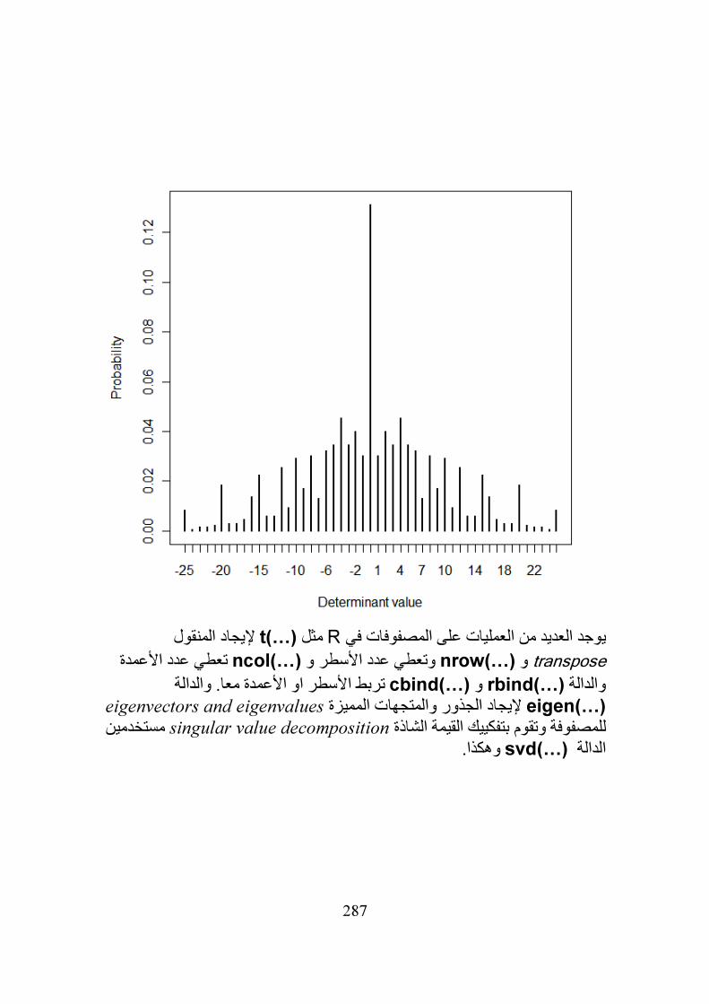
287
إليجاد المنقول (…)tمثل Rعلى المصفوفات في يوجد العديد من العملياتtranspose وnrow(…) وتعطي عدد األسطر وncol(…) تعطي عدد األعمدة
تربط األسطر او األعمدة معا. والدالة (…)cbindو (…)rbindوالدالة eigen(…) ميزة إليجاد الجذور والمتجهات المeigenvectors and eigenvalues
ستخدمين م singular value decompositionبتفكييك القيمة الشاذة صفوفة وتقومللم وهكذا. (…)svdالدالة

288
:Data from the Internetإدخال بيانات من اإلنترنت
لجلب وإدخال بيانات من اإلنترنت كالتالي: ()read.tableنستخدم
> data <-read.table("http://www.stat.ucla.edu/~vlew
/stat130a/datasets/twins.csv",header=TRUE,sep=",")
بأن البيانات تشمل أسماء المتغيرات في أول Rتخبر header=TRUEحيث سطر.
) ." ," أن البيانات مفصولة بواسطة فاصلة ( Rتخبر ","=sepو
289
Quick R دليل العمل:
Working directory: setwd("../scripts") getwd()
المساعدة:Help: help(x) ?x help.search("x") help.start() demo() demo(graphics)
تثبيت وتحميل الحزم:Installing and loading the package: install.packages("spuRs") library(spuRs)
العمليات الحسابية:Arithmetic: (1 + 1/100)^100 17%%5 17%/%5 exp(1) options(digits = 16) exp(1) pi sin(pi/6)
المتغيرات:Variables: x <- 100 x (1 + 1/x)^x x <- 200 (1 + 1/x)^x (y <- (1 + 1/x)^x) n <- 1 n <- n + 1 n
الدوال:Functions:

290
seq(from = 1, to = 9, by = 2) seq(from = 1, to = 9) seq(1, 9, 2) seq(to = 9, from = 1) seq(by = -2, 9, 1) x <- 9 seq(1, x, x/3)
291
المتجهات:Vectors: (x <- seq(1, 20, by = 2)) (y <- rep(3, 4)) (z <- c(y, x)) (x <- 100:110) i <- c(1, 3, 2) x[i] j <- c(-1, -2, -3) x[j] x <- c() length(x)
العمليات الجبرية على المتجهات:Algebraic operations on vectors: x <- c(1, 2, 3) y <- c(4, 5, 6) x * y x + y y^x c(1, 2, 3, 4) + c(1, 2) (1:10)^c(1, 2) 2 + c(1, 2, 3) 2 * c(1, 2, 3) (1:10)^2 sqrt(1:6) mean(1:6) sort(c(5, 1, 3, 4, 2))
مثال: المتوسط و التباينExample: mean and variance x <- c(1.2, 0.9, 0.8, 1, 1.2) x.mean <- sum(x)/length(x) x.mean - mean(x) x.var <- sum((x - x.mean)^2)/(length(x) - 1) x.var - var(x)
مثال: تكامل عددي بسيطExample: simple numerical integration dt <- 0.005 t <- seq(0, pi/6, by = dt) ft <- cos(t) (I <- sum(ft) * dt) I - sin(pi/6)
مثال: النهايات االسية

292
Example: exponential limit x <- seq(10, 200, by = 10) y <- (1 + 1/x)^x plot(x, y)
القيم المفقودة:Missing data: a <- NA # assign NA to variable A is.na(a) # is it missing? a <- c(11,NA,13) # now try a vector is.na(a) # is it missing? mean(a) # NAs can propagate mean(a, na.rm = TRUE) # NAs can be removed
المصفوفات:
Matrices: (A <- matrix(1:6, nrow = 2, ncol = 3, byrow = TRUE)) A[1, 3] <- 0 A[, 2:3] (B <- diag(c(1, 2, 3))) (A <- matrix(c(3, 5, 2, 3), nrow = 2, ncol = 2)) (B <- matrix(c(1, 1, 0, 1), nrow = 2, ncol = 2)) A %*% B A * B (A.inv <- solve(A)) A %*% A.inv A^(-1) A[2] is.matrix(x) is.vector(x) A <- as.matrix(x) as.vector(A)
فضاء العمل:The workspace: ls() objects() rm(x) rm(list = ls()) save.image(file = "fname") save(x, y, file = "fname")
293
load(file = "fname") savehistory(file = "fname") loadhistory(file = "fname")
برمجة أساسية:Basic programming: # find the zeros of a2*x^2 + a1*x + a0 = 0 # clear the workspace rm(list=ls()) # input a2 <- 1 a1 <- 4 a0 <- 2 # calculation root1 <- (-a1 + sqrt(a1^2 - 4*a2*a0))/(2*a2) root2 <- (-a1 - sqrt(a1^2 - 4*a2*a0))/(2*a2) # output show(c(root1, root2))
:ifالتشعب بواسطة Branching with if: if (logical_expression) { expression_1 ... } if (logical_expression) { expression_1 ... } else { expression_2 ... }
مثال: جذور المعادلة التربيعيةExample: roots of a quadratic # find the zeros of a2*x^2 + a1*x + a0 = 0 # clear the workspace rm(list=ls()) # input a2 <- 1 a1 <- 4 a0 <- 5 # calculate the discriminant discrim <- a1^2 - 4*a2*a0 # calculate the roots depending on the value of the discriminant
294
if (discrim > 0) { roots <- c( (-a1 + sqrt(a1^2 - 4*a2*a0))/(2*a2), (-a1 - sqrt(a1^2 - 4*a2*a0))/(2*a2) ) } else { if (discrim == 0) { roots <- -a1/(2*a2) } else { roots <- c() } } # output show(roots)
:forبواسطة الدوران Looping with for: for (x in vector) { expression_1 ... }
مثال: جمع عناصر متجهExample: summing a vector (x_list <- seq(1, 9, by = 2)) sum_x <- 0 for (x in x_list) { + sum_x <- sum_x + x + cat("The current loop element is", x, "\n") + cat("The cumulative total is", sum_x, "\n") + } sum(x_list)
:nمضروب
Example: n factorial # Calculate n factorial # clear the workspace rm(list=ls()) # Input n <- 6 # Calculation n_factorial <- 1 for (i in 1:n) { n_factorial <- n_factorial * i } # Output

295
show(n_factorial)
:whileالدران بواسطة
Looping with while: while (logical_expression) { expression_1 ... }
مثال: ارقام فيبونتشيExample: Fibonacci numbers
رف تكرايا من القاعدةوالتي تع F1F ,2 ,. . . ,لنعتبر أرقام فيبونتشي F1 = 1, F2 = 1, Fn = Fn−1 + Fn−2 for n ≥ 2.
البرنامج:# calculate the first Fibonacci number greater than 100 # clear the workspace rm(list=ls()) # initialise variables F <- c(1, 1) # list of Fibonacci numbers n <- 2 # length of F # iteratively calculate new Fibonacci numbers while (F[n] <= 100) { # cat("n =", n, " F[n] =", F[n], "\n") n <- n + 1 F[n] <- F[n-1] + F[n-2] } # output cat("The first Fibonacci number > 100 is F(", n, ") =", F[n], "\n") F
البرمجة المعتمدة على المتجه:
Vector-based programming: عدد بإستخدام الدوران nمثال: جمع مربعات أول
Example: sum of the first n squares using a loop n <- 100 S <- 0 for (i in 1:n) { + S <- S + i^2 + }

296
S
عدد بإستخدام العمليات المتجهية nمثال: جمع مربعات أول Example: sum of the first n squares using vector operations: sum((1:n)^2) ifelse: ifelse(test, A, B) x <- c(-2, -1, 1, 2) ifelse(x > 0, "Positive", "Negative")
pmin and pmax:
maxو minوهي الشكل المتجهي للدوال pmin(c(1, 2, 3), c(3, 2, 1), c(2, 2, 2))
اإلدخال من ملف:
Input from a file: list.files(path = "dir.name") scan(file = "", what = 0, n = -1, sep = "", skip = 0, quiet = FALSE)
مثال: إدخال من ملفExample: file input # Calculate median and quartiles. # Clear the workspace rm(list=ls()) # Input # We assume that the file file_name consists of numeric values # separated by spaces and/or newlines file_name = "../data/data1.txt" # Read from file data <- scan(file = file_name) # Calculations n <- length(data) data.sort <- sort(data) data.1qrt <- data.sort[ceiling(n/4)] data.med <- data.sort[ceiling(n/2)] data.3qrt <- data.sort[ceiling(3*n/4)]

297
# Output cat("1st Quartile:", data.1qrt, "\n") cat("Median: ", data.med, "\n") cat("3rd Quartile:", data.3qrt, "\n")
OR: quantile(scan("../data/data1.txt"), (0:4)/4)

298
إدخال من لوحة المفاتيح:Input from the keyboard:
مثال: جذور المعادلة التربيعيةExample: roots of a quadratic # find the zeros of a2*x^2 + a1*x + a0 = 0 # clear the workspace rm(list=ls()) # input cat("find the zeros of a2*x^2 + a1*x + a0 = 0\n") a2 <- as.numeric(readline("a2 = ")) a1 <- as.numeric(readline("a1 = ")) a0 <- as.numeric(readline("a0 = ")) # calculate the discriminant discrim <- a1^2 - 4*a2*a0 # calculate the roots depending on the value of the discriminant if (discrim > 0) { roots <- (-a1 + c(1,-1) * sqrt(a1^2 - 4*a2*a0))/(2*a2) } else { if (discrim == 0) { roots <- -a1/(2*a2) } else { roots <- c() } } # output if (length(roots) == 0) { cat("no roots\n") } else if (length(roots) == 1) { cat("single root at", roots, "\n") } else { cat("roots at", roots[1], "and", roots[2], "\n") }
اإلخراج لملف:
Output to a file: write(x, file = "data", ncolumns = if(is.character(x)) 1 else 5, append = FALSE) (x <- matrix(1:24, nrow = 4, ncol = 6)) write(t(x), file = "../results/out.txt", ncolumns = 6) cat(..., file = "", sep = " ", append = FALSE)
299
dump("x", file = "../results/x.txt")
الرسم:Plotting: plot(x, y, type)
مثال:Example: x <- seq(0, 5, by = 0.01) y.upper <- 2 * sqrt(x) y.lower <- -2 * sqrt(x) y.max <- max(y.upper) y.min <- min(y.lower) plot(c(-2, 5), c(y.min, y.max), type = "n", xlab = "x", + ylab = "y") lines(x, y.upper) lines(x, y.lower) abline(v = -1) points(1, 0) text(1, 0, "focus (1, 0)", pos = 4) text(-1, y.min, "directrix x = -1", pos = 4) title("The parabola y^2 = 4*x")
عدة رسومات:Multiple graphs: par(mfrow = c(nr, nc)) par(mfcol = c(nr, nc))
مثال:example: par(mfrow = c(2, 2)) curve(x * sin(x), from = 0, to = 100, n = 1001) curve(x * sin(x), from = 0, to = 10, n = 1001) curve(x * sin(x), from = 0, to = 1, n = 1001) curve(x * sin(x), from = 0, to = 0.1, n = 1001) par(mfrow = c(1, 1))
البرمجة بالدوال:Programming with functions:
الدوال:Functions:
الدالة لها الشكل:name <- function(argument_1, argument_2, ...) {
300
expression_1 expression_2 ... return(output) }
إلستخدام (نداء) أو إجراء دالةname(x1, x2, ...)
دلة التربيعيةمثال: جذور المعاExample: roots of a quadratic quad3 <- function(a0, a1, a2) { # find the zeros of a2*x^2 + a1*x + a0 = 0 if (a2 == 0 && a1 == 0 && a0 == 0) { roots <- NA } else if (a2 == 0 && a1 == 0) { roots <- NULL } else if (a2 == 0) { roots <- -a0/a1 } else { # calculate the discriminant discrim <- a1^2 - 4*a2*a0 # calculate the roots depending on the value of the discriminant if (discrim > 0) { roots <- (-a1 + c(1,-1) * sqrt(a1^2 - 4*a2*a0))/(2*a2) } else if (discrim == 0) { roots <- -a1/(2*a2) } else { roots <- NULL } } return(roots) }
المخرج:
output: rm(list = ls()) quad3(1, 0, -1) quad3(1, -2, 1) quad3(1, 1, 1)
( توافيق) rإختيار nمثال:
Example: n choose r n_factorial <- function(n) {
301
# Calculate n factorial n_fact <- prod(1:n) return(n_fact) } n_choose_r <- function(n, r) { # Calculate n choose r n_ch_r <- n_factorial(n)/n_factorial(r)/n_factorial(n-r) return(n_ch_r) }
المخرج:output: rm(list = ls()) n_choose_r(4, 2) n_choose_r(6, 4)
الصعيد:
Scope: Argumentsالحجج و المتغيرات Variable اجد فقط ضمن تلك الدالةداخل دالة تتو xأي اننا لو عرفنا وأستخدمنا المتغير داخل دالة فهذا المتغير اليكون له وجود خارج تلك الدالة. إذا وجدت متغيرات لها نفس اإلسم داخل وخارج دالة فهذان المتغيرين مختلفان تماما وليس بينهما أي صلة.
مثال توضيحي:Illustration: test <- function(x) { + y <- x + 1 + return(y) + } test(1) [1] 2 x Error: Object "x" not found y Error: Object "y" not found y <- 10 test(1)
302
[1] 2 y [1] 10
The variableجزء البرنامج والذي يكون متغير معرف ضمنه يسمى صعيده scope تها خارج الدالة و العكس صحيح.المتغيرات المعرفة داخل دالة ليمكن رؤي
مثال:test2 <- function(x) { + y <- x + z + return(y) + } z <- 1 test2(1) [1] 2 z <- 2 test2(1) [1] 3
الحجج اإلختيارية والقيم اإلفتراضية:
Optional arguments and default values: argument_1 = x1نستخدم x1القيمة اإلفتراضية argument_1إلعطاء الحجة
داخل معرف الدالة.R .يسند حجج للمتغيرات من اليسار إال إذا سميت الحجة
مثال توضيحي:Illustration: test3 <- function(x = 1, y = 1, z = 1) { + return(x * 100 + y * 10 + z) + } test3(2, 2) [1] 221 test3(y = 2, z = 2) [1] 122
303
المتجهية بإستخدام الدوال: البرمجةVector-based programming using functions:
أي إذا اعطي مدخل متجهي فإن Functions Vectorisedمتجهية Rكثير من دوال الدالة تعمل على كل عنصر منفصال في المتجة ويعاد مخرج متجهي. ويعد هذا صفة
وسهل القرائة.والتي تسمح بوضع برنامج مدمج وفعال Rقوية لـ عائلة من الدوال القوية والمرنة والتي تمكن من Rلتسهيل البرمجة المتجهية يوجد في
الدوال المعرفة بالمستخدم: Vectorisationتوجيه apply, sapply, lapply, tapply, and mapply.
على كل عنصر من عناصر FUNتطبيق الدالة sapply(X, FUN)تأثير قيمة iتعيد متجه يكون عنصره رقم sapply(X, FUN) أي أن Xالمتجه فإنه X[i]حجج اخرى غير FUNإذا كان للدالة FUN(X[i])التعبير
والتي تعيد sapply(X, FUN, ...)باإلمكان شملها بإستخدام FUN(X[i], ...) كعنصرها رقمi. لتتجيه أكثر من حجة واحدة نستخدم
mapply.
ذ حجج متجهية لكل من األسطر (أو األعمدة) لمصفوفة عندا إذا اردنا نطبيق دالة تأخ .applyنستخدم الدالة
: كثافة األعداد األوليةمثالExample: density of primes
سوف نكتب دالة والتي تختبر إذا كان عدد صحيح معطى أولي أو ال. ثم نستخدم sapply 2 لنطبق الدالة على المتجه:n األولية التي أقل وبهذا نعرف كل األعداد
.n من أو تساوي كمتجه. xوالتي تعطي المجوع التراكمي لـ cumsum(x)سوف نستخدم الدالة
ليصبح Rوالذي تجبره TRUE/FALSEسوف نطبقه على متجه منطقي يحوي قيم ) قبل حساب المجمع التراكمي.R coerces into a 1/0 vector(أي 1/0متجه
# estimate the density of primes (using a very inefficient algorithm) # clear the workspace rm(list=ls()) prime <- function(n) { # returns TRUE if n is prime # assumes n is a positive integer if (n == 1) { is.prime <- FALSE } else if (n == 2) { is.prime <- TRUE } else { is.prime <- TRUE
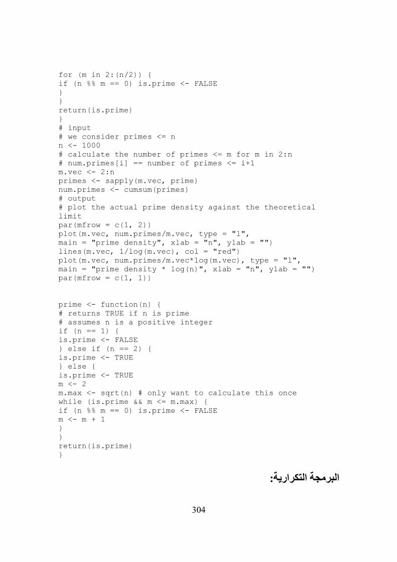
304
for (m in 2:(n/2)) { if (n %% m == 0) is.prime <- FALSE } } return(is.prime) } # input # we consider primes <= n n <- 1000 # calculate the number of primes <= m for m in 2:n # num.primes[i] == number of primes <= i+1 m.vec <- 2:n primes <- sapply(m.vec, prime) num.primes <- cumsum(primes) # output # plot the actual prime density against the theoretical limit par(mfrow = c(1, 2)) plot(m.vec, num.primes/m.vec, type = "l", main = "prime density", xlab = "n", ylab = "") lines(m.vec, 1/log(m.vec), col = "red") plot(m.vec, num.primes/m.vec*log(m.vec), type = "l", main = "prime density * log(n)", xlab = "n", ylab = "") par(mfrow = c(1, 1)) prime <- function(n) { # returns TRUE if n is prime # assumes n is a positive integer if (n == 1) { is.prime <- FALSE } else if (n == 2) { is.prime <- TRUE } else { is.prime <- TRUE m <- 2 m.max <- sqrt(n) # only want to calculate this once while (is.prime && m <= m.max) { if (n %% m == 0) is.prime <- FALSE m <- m + 1 } } return(is.prime) }
البرمجة التكرارية:

305
Recursive programming: البرنامج التكراري هو ببساطة البرنامج الذي يستخدم نفسه. وهذه الخاصية مفيدة ألن
الكثير من الخوارزمات تكرارية بطبيعتها. nمثال: مضروب
Example: n factorial nfact2 <- function(n) { # calculate n factorial if (n == 1) { cat("called nfact2(1)\n") return(1) } else { cat("called nfact2(", n, ")\n", sep = "") return(n*nfact2(n-1)) } } nfact2(6) called nfact2(6) called nfact2(5) called nfact2(4) called nfact2(3) called nfact2(2) called nfact2(1) [1] 720
مثال: منخل ( مصفاة أو فلتر) إراتوسثيينExample: Sieve of Eratosthenes منخل إراتوسثيين هو عبارة عن خوارزم إليجاد كل األعداد األولية التي هي أقل من أو
.nتساوي عدد معطى primesieve <- function(sieved, unsieved) { # finds primes using the Sieve of Eratosthenes # sieved: sorted vector of sieved numbers # unsieved: sorted vector of unsieved numbers # cat("sieved", sieved, "\n") # cat("unsieved", unsieved, "\n") p <- unsieved[1] n <- unsieved[length(unsieved)] if (p^2 > n) { return(c(sieved, unsieved)) } else { unsieved <- unsieved[unsieved %% p != 0] sieved <- c(sieved, p)
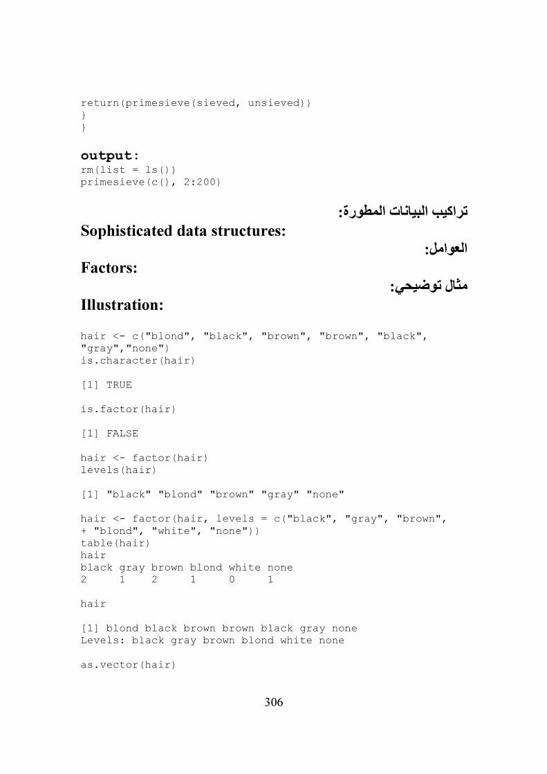
306
return(primesieve(sieved, unsieved)) } }
output: rm(list = ls()) primesieve(c(), 2:200)
تراكيب البيانات المطورة:Sophisticated data structures:
العوامل:Factors:
مثال توضيحي:Illustration: hair <- c("blond", "black", "brown", "brown", "black", "gray","none") is.character(hair) [1] TRUE is.factor(hair) [1] FALSE hair <- factor(hair) levels(hair) [1] "black" "blond" "brown" "gray" "none" hair <- factor(hair, levels = c("black", "gray", "brown", + "blond", "white", "none")) table(hair) hair black gray brown blond white none 2 1 2 1 0 1 hair [1] blond black brown brown black gray none Levels: black gray brown blond white none as.vector(hair)

307
[1] "blond" "black" "brown" "brown" "black" "gray" "none" as.numeric(hair) [1] 4 1 3 3 1 2 6 c(hair, 5) [1] 4 1 3 3 1 2 6 5 x <- factor(c(0.8, 1.1, 0.7, 1.4, 1.4, 0.9)) as.numeric(x) # does not recover x [1] 2 4 1 5 5 3 as.numeric(levels(x))[x] # does recover x [1] 0.8 1.1 0.7 1.4 1.4 0.9 as.numeric(as.character(x)) # does recover x [1] 0.8 1.1 0.7 1.4 1.4 0.9 table(hair[hair == "gray" | hair == "none"]) black gray brown blond white none 0 1 0 0 0 1 table(hair[hair == "gray" | hair == "none", drop = TRUE]) gray none 1 1
مثال توضيحي:Illustration: phys.act <- c("L", "H", "H", "L", "M", "M") phys.act <- factor(phys.act, levels = c("L", "M", "H"), + ordered = TRUE) is.ordered(phys.act) [1] TRUE phys.act[2] > phys.act[1] [1] TRUE

308
phys.act <- factor(phys.act, levels = c("L", "M", "H"), + labels = c("Low", "Medium", "High"), ordered = TRUE) table(phys.act) phys.act Low Medium High 2 2 2 which(phys.act == "High") [1] 2 3
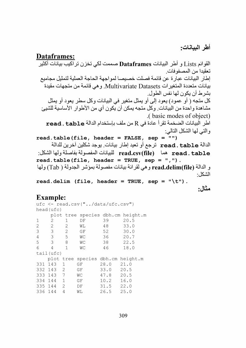
309
أطر البيانات:Dataframes:
صممت لكي تخزن تراكيب بيانات أكثير Dataframesو أطر البيانات Listsالقوائم وفات. تعقيدا من المصف
إطار البيانات عبارة عن قائمة فصلت خصيصا لمواجهة الحاجة العملية لتمثيل مجاميع . وهي قائمة من متجهات مقيدة Multivariate Datasetsبيانات متعددة المتغيرات
بشرط أن يكون لها نفس الطول.مثل كل متجه ( أو عمود) يعود إلى أو يمثل متغير في البيانات وكل سطر يعود أو ي
مشاهدة واحدة من البيانات. وكل متجه يمكن أن يكون أي من األطوار األساسية للشيئ )basic modes of object .(
read.tableمن ملف بإستخدام الدالة Rاطر البيانات الضخمة تقرأ عادة في
والتي لها الشكل التالي:read.table(file, header = FALSE, sep = "")
ترجع أو تعيد إطار بيانات. يوجد شكلين آخرين للدالة read.tableالدالة read.table هما read.csv(file) :للبيانات المفصولة بفاصلة ولها الشكل
read.table(file, header = TRUE, sep = ","). ) ولها Tabوهي لقرائة بيانات مفصولة بمؤشر الجدولة ( read.delim(file) و الدالة الشكل:
read.delim (file, header = TRUE, sep = "\t").
:مثال Example: ufc <- read.csv("../data/ufc.csv") head(ufc) plot tree species dbh.cm height.m 1 2 1 DF 39 20.5 2 2 2 WL 48 33.0 3 3 2 GF 52 30.0 4 3 5 WC 36 20.7 5 3 8 WC 38 22.5 6 4 1 WC 46 18.0 tail(ufc) plot tree species dbh.cm height.m 331 143 1 GF 28.0 21.0 332 143 2 GF 33.0 20.5 333 143 7 WC 47.8 20.5 334 144 1 GF 10.2 16.0 335 144 2 DF 31.5 22.0 336 144 4 WL 26.5 25.0

310
كل عمود أو متغير في إطار البيانات له إسم وحيد ونستطيع إستخراج هذا المتغير بواسطة إسم إطار البيانات وإسم العمود وبينهم عالمة الدوالر أي
x <- ufc$height.m x[1:5] [1] 20.5 33.0 30.0 20.7 22.5
متكافئة ufc[["height.m"]]و ufc$height.m, ufc[[5]]األشكال ويمكن إستخراج عناصر من إطار البيانات مباشرة بإستخدام مؤشر مصفوفي
ufc[1:5, 5] [1] 20.5 33.0 30.0 20.7 22.5
.ufc[c("dbh.cm", "height.m")]مكافئ لـ ufc[4:5]التأشير diam.height <- ufc[4:5] diam.height[1:5, ] dbh.cm height.m 1 39 20.5 2 48 33.0 3 52 30.0 4 36 20.7 5 38 22.5 is.data.frame(diam.height) [1] TRUE mode(ufc) [1] "list" mode(ufc[5]) [1] "list" mode(ufc[[5]]) [1] "numeric"
نا تكوين إطار بيانات من مجموعة من إضافة لقرائة إطار بيانات من ملف فإنه يمكنوالتي لها data.frameالمتجهات و/أو اطربيانات موجودة سابقا بإستخدام الدالة
الشكل:data.frame(col1 = x1, col2 = x2, ..., df1, df2,
...)
الخ هي اسماء اعمدة ( وتكتب كحروف بدون عالمات إقتباس col2 و col1هنااطر بيانات df2 و df1الخ متجهات لها نفس الطول و x2 و x1) و '" أو
.x2 و x1والتي يجب ان تكون اطوال اعمدتها نفس اطوال
ايضا يمكننا إضافة متغير داخل اطار بيانات بإعطائه إسم و إسناد قيمة له. مثال:
ufc$volume.m3 <- pi * (ufc$dbh.cm/200)^2 * ufc$height/2 mean(ufc$volume.m3) [1] 1.93294

311
الحظ ان:ufc$volume.m3 و ufc[6] و ufc["volume.m3"] و ufc[[6]]
جميعها متكافئة. ufc[["volume.m3"]] وكمتجه من الحروف. لتغيير األسماء dfيعطي أسماء إطار البيانات names(df)األمر
نعيد إسناد اسماء جديدة لها مثل:(ufc.names <- names(ufc)) [1] "plot" "tree" "species" "dbh.cm" "height.m" [6] "volume.m3" names(ufc) <- c("P", "T", "S", "D", "H", "V") names(ufc) [1] "P" "T" "S" "D" "H" "V" names(ufc) <- ufc.names
صفات إطار البيانات:Dataframe attributes: names(df) dim(df) row.names(df)
:subsetالدالة
The function subset: fir.height <- subset(ufc, subset = species %in% c("DF", "GF"), + select = c(plot, tree, height.m)) head(fir.height) plot tree height.m 1 2 1 20.5 3 3 2 30.0 7 4 2 17.0 8 5 2 29.3 9 5 4 29.0 10 6 1 26.0
يعطي متجة منطقي له x %in% yلتعبير والذين لهم نفس الطور ا yو xللمتجهين عنصر من x[i]فقط وفقط إذا كان TRUEيكون iوعنصرة الـ xنفس طول
.yعناصر
لكتابة إطار بيانات في ملف نستخدم:To write a dataframe to a file we use write.table(x, file = "", append = FALSE, sep = " ", row.names = TRUE, col.names = TRUE)

312
.na.omitويمكن إزالة األسطر التي تحوي قيم مفقودة بإستخدام الدالة
التوصيل:Attaching:
لتوصيل اطار بيانات لفضاء عمل attach(ufc) max(height.m[species == "GF"]) [1] 47
ولفصلهheight.m <- 0 #vandalism max(height.m) [1] 0 max(ufc$height.m) [1] 47 detach(ufc) max(ufc$height.m) [1] 47
القوائم:Lists:
من األشياء وجميع عناصره Indexed setلقد ذكرنا أن المتجة هو مجموعة مفهرسة أو مجدولة
المتجه. Modeلها نفس النوع ( عددي أو حرفي أو منطقي ألخ) والذي سميناة نوع
ها بعكس المتجه فإن عناصرها يمكن أن تكون القائمة هي أيضا مجموعة مفهرسة من األشياء ولكن
لتجميع Rمن أنواع مختلفة وقد تضمن قوائم اخرى ونوع القائمة هو قائمة وتستخدم القوائم في
وتخزين مخرجات دوال معقدة. الحظ أن أطر البيانات هي حالة خاصة من القوائم.
بحجج مفصولة بفواصل. (…)listتولد الفائمة بإستخدام األمر
تستخدم األقواس المربعة المفردة إلختيار قوائم فرعية أو ثانوية و األقواس المربعة المضاعفة
إلختيار عنصر واحد.
أمثلة:
Examples:
> my.list <- list("one", TRUE, 3, c("f", "o", "u", "r"))
> my.list[[2]]
[1] TRUE
> mode(my.list[[2]])

313
[1] "logical"
> my.list[2]
[[1]]
[1] TRUE
> mode(my.list[2])
[1] "list"
> my.list[[4]][1]
[1] "f"
> my.list[4][1]
[[1]]
[1] "f" "o" "u" "r"
الخ لتبين عناصر القائمة و [[2]]و [[1]]أقواس مربعة مضاعفة Rعندما تعرض قائمة تستخدم
الخ لتبين عناصر المتجه. [2]و [1]أقواس مربعة وحيدة
> my.list <- list(first = "one", second = TRUE, third = 3,
+ fourth = c("f", "o", "u", "r"))
> names(my.list)
[1] "first" "second" "third" "fourth"
> my.list$second
[1] TRUE
> names(my.list) <- c("First element", "Second element",
+ "Third element", "Fourth element")
> my.list$"Second element"
[1] TRUE
> x <- "Second element"
> my.list[[x]]
[1] TRUE
unlist(x)لتمهيد قائمة أي تحويلها إلى متجة نستخدم األمر

314
> x <- list(1, c(2, 3), c(4, 5, 6))
> unlist(x)
[1] 1 2 3 4 5 6
القوائم تمهد أيضا إال إذا أمرنا بغير ذلك بإستخدام إذا كانت القائمة تحوي قوائم داخلها فإن هذه
.recursive = FALSEالحجة
> lm.xy <- lm(y ~ x, data = data.frame(x = 1:5, y = 1:5))
> mode(lm.xy)
[1] "list"
> names(lm.xy)
[1] "coefficients" "residuals" "effects" "rank"
[5] "fitted.values" "assign" "qr" "df.residual"
[9] "xlevels" "call" "terms" "model"
أعادة قائمة. العنصر األول lmالحظ هنا اليهمنا كيفية تطبيق الخط المستقيم ولكن نالحظ أن الدلة
متجه يعطي قيم residualsوالثاني المسمى bو aهو متجة يعطي coefficientsالمسمى
b - ia x - iy لجميع قيمi والمسمى الثالثfitted.values متجه يعطي+ b ia x .وهكذا
applyعائلة
The apply family
العديد من التقنيات لمعالجة القوائم و اطر البيانات منها عدة دوال والتي تمكن من Rيوجد في
تطبيق دالة على جميع عناصر ( أو مجموعة مختارة ) القائمة او اطار البيانات.
tapplyالدالة
لها التركيب التالي:و
tapply(X, INDEX, FUN, ...),
حيث الحجج:
X .المتجه الذي ستطبق عليه الدالة

315
INDEX عاملfactor له نفس طولX ) والذي يستخدم لتجميعgroupعناصر (
X.
FUN .الدلة المطبقة
sapplyو lapplyتطبيق دوال على قوائم بإستخدام
Applying functions to lists lapply and sapply
مثال يمكن حساب arrayلتطبيق دالة على متجه أو صف applyو sapplyيمكن إستخدام
مجاميع األسط و األعمدة لمصفوفة.
تطبق lapply(X,FUN,…). الدالة lappyأو sapplyلتطبيق دالة على قائمة نستخدم إما
تطبق sapply(X,FUN,…)وتعطي قائمة. الدالة Xعلى جميع عناصر القائمة FUNالدالة
قائمة أو متجه. Xسواء كانت Xعلى جميع عناصر FUNالدالة
316
:Rفي اإلحصائية مكاناتمقدمة لإل
بعض الدوال واألوامر األولية:
إضافة حزمة install.packages('ggplot2')
install.packages("Rcmdr")
لتحميل حزمة للعمل بدوالها
library(ggplot2) لتجديد الحزم
update.packages()
للمساعدة لمعرفة إستخدام دالةhelp(functionname)
meanطريقتين للمساعدة عن إستخدام help(mean) ?mean
للمساعدة في معرفة حجج دالةargs(functionname)
argsمثال إلستخدام args(mean) function (x, ...) NULL args(sd) function (x, na.rm = FALSE) NULL
إعطاء مثال إلستخدام دالةexample(functionname) example(mean) mean> x <- c(0:10, 50) mean> xm <- mean(x) mean> c(xm, mean(x, trim = 0.1)) [1] 8.75 5.50

317
mean> mean(USArrests, trim = 0.2) Murder Assault UrbanPop Rape 7.42 167.60 66.20 20.16
Rاجر هذا األمر لتوجه لصفحة تعطي كتيبات ومراجع و أشياء اخرى عن
help.start() Rللبحث عن أمر في مواقع
http://rseek.org http://stackoverflow.com/ http://stats.stackexchange.com/ RSiteSearch("key phrase")
مثالRSiteSearch("canonical correlation")
لمعرفة دليل العمل الحاليgetwd()
لتحديد دليل عملsetwd("R:\\data") setwd("R:/data")
لسرد محتويات دليل العمل dir()

318
إدخال بيانات:
dfrmقرائة بيانات على شكل جدول ووضعها في مجموعة بيانات تسمى dfrm = read.table("filename.txt")
المث
dfrm = read.table("statisticians.txt", sep=" ")
(مثال يحوي بيانات رقمية ونصية statisticians.txtتقرأ بيانات من الملف النصي الخ)
والذي نستخدمه عن طريق dfrmالموجود في مجموعة البيانات V1لمعرفة صنف المتغير dfrm$V1التأشير له
class(dfrm$V1)
لف يحوي السطر أسماء المتغيرات للقرائة من م
dfrm = read.table("statisticians.txt", header=TRUE)
csvللقرائة من ملف
tbl = read.csv("filename")
اليحوي أسماء متغيرات csvللقرائة من ملف
tbl = read.csv("filename", header=FALSE)
للقرائة من ملف يختار من مجلد
data = read.csv(file.choose(), header = TRUE)
للقرائة من ملف على اإلنترنتhs0 <- read.table("http://www.ats.ucla.edu/stat/R/notes/hs0.csv", header=T, sep=",")
قرائة بيانات اخرى من اإلنترنت data = read.csv("http://wiki.stdout.org/rcookbook/Data input and output/Loading data from a file/datafile.csv") data
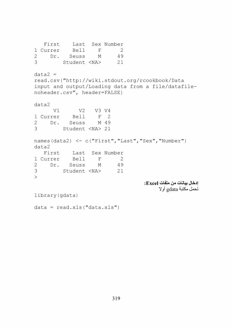
319
First Last Sex Number 1 Currer Bell F 2 2 Dr. Seuss M 49 3 Student <NA> 21 data2 = read.csv("http://wiki.stdout.org/rcookbook/Data input and output/Loading data from a file/datafile-noheader.csv", header=FALSE) data2 V1 V2 V3 V4 1 Currer Bell F 2 2 Dr. Seuss M 49 3 Student <NA> 21 names(data2) <- c("First","Last","Sex","Number") data2 First Last Sex Number 1 Currer Bell F 2 2 Dr. Seuss M 49 3 Student <NA> 21 >
:Excel إدخال بيانات من ملفات أوال gdataتحمل مكتبة
library(gdata) data = read.xls("data.xls")

320
SASو SPSSإدخال بيانات من ملفات أوال foreignتحمل مكتبة
library(foreign) data = read.spss("data.sav", to.data.frame=TRUE) data = read.sas("data.sas", to.data.frame=TRUE)
إدخال بيانات من لوحة المفاتيح أو لوحة النسخ
data = read.csv(stdin()) data = read.table(stdin(), header=TRUE) data = read.csv('clipboard') data = read.table('clipboard', header=TRUE)
مثال:
a<-read.csv(stdin()) gender,id,race,ses,schtyp,prgtype,read,write,math,science,socst 0,70,4,1,1,general,57,52,41,47,57 1,121,4,2,1,vocati,68,59,53,63,61 0,86,4,3,1,general,44,33,54,58,31 0,141,4,3,1,vocati,63,44,47,53,56
طباعة البيانات
print(data, row.names=FALSE)
كتابة البيانات إلى لوحة النسخ أو للشاشة
write.csv(df, 'clipboard', row.names=FALSE) write.csv(data, stdout(), row.names=FALSE)
تخزين البيانات
write.csv(data, "data.csv", row.names=FALSE) write.table(data, "data.csv", sep="\t", row.names=FALSE, col.names=FALSE) write.csv(data, "data.csv", row.names=FALSE, na="")

321
تخزين البيانات في شكل نصي ثم إسترجاعهاdump("data", "data.Rdmpd") source("data.Rdmpd")
ثم إسترجاعها Rتخزين البيانات في شكل خاص بـ
save("data", file="data.RData") load("data.RData")

322
معالجة المتغيرات
إدخال قيم بشكل متجه (بدون حفظ القيم)c(1,1,2,3,5,8,13,21)
v2و v1إدخال قيم بشكل متجه وحفظها في v1 = c(1,2,3) v2 = c(4,5,6)
(بدون حفظ القيم) v2و v1ضم المتجهين c(v1,v2)
xإدخال بيانات في متجه x = c(0,1,1,2,3,5,8,13,21,34)
(بدون حفظ القيمة) xإيجاد متوسط mean(x) [1] 8.8
(بدون حفظ القيمة) xإيجاد وسيط median(x) [1] 4
(بدون حفظ القيمة) xإيجاد اإلنحراف المعياري لـ sd(x) [1] 11.03328
(بدون حفظ القيمة) xإيجاد تباين var(x) [1] 121.7333
yو تحفظ في المتجة xإيجاد دالة من y <- log(x+1)
yمع xإيجاد ترابط cor(x,y) [1] 0.9068053
yمع xإيجاد تغاير cov(x,y) [1] 11.49988
Rوالتي يرمز لها في missing value(يستبدل المتجه السابق) يحوي قيمة مفقودة xمتجه جديد NAبالرمز
x <- c(0,1,1,2,3,NA) NAالمعياري تعطي الحظ أن دالتي المتوسط و اإلنحراف
mean(x) [1] NA sd(x) [1] NA

323
أي إستبعاد القيم المفقودة نتحصل على القيم للدوال na.rm=TRUEبإعطاء األمر الجانبي المطلوبة بعد إزالة القيم المفقودة
mean(x, na.rm=TRUE) [1] 1.4 sd(x, na.rm=TRUE) [1] 1.140175
dframeلمشاهدة البيانات في المجموعة print(dframe) small medium big 1 0.6739635 10.526448 99.83624 2 1.5524619 9.205156 100.70852 3 0.3250562 11.427756 99.73202 4 1.2143595 8.533180 98.53608 5 1.3107692 9.763317 100.74444 6 2.1739663 9.806662 98.58961 7 1.6187899 9.150245 100.46707 8 0.8872657 10.058465 99.88068 9 1.9170283 9.182330 100.46724 10 0.7767406 7.949692 100.49814
dframeحساب إحصائآت المتغيرات في المجموعة
summary(dframe) mean(dframe) small medium big 1.245040 9.560325 99.946003 sd(dframe) small medium big 0.5844025 0.9920281 0.8135498 var(dframe) small medium big small 0.34152627 -0.21516416 -0.04005275 medium -0.21516416 0.98411974 -0.09253855 big -0.04005275 -0.09253855 0.66186326 cor(dframe) small medium big small 1.00000000 -0.3711367 -0.08424345

324
medium -0.37113670 1.0000000 -0.11466070 big -0.08424345 -0.1146607 1.00000000 cov(dframe) small medium big small 0.34152627 -0.21516416 -0.04005275 medium -0.21516416 0.98411974 -0.09253855 big -0.04005275 -0.09253855 0.66186326
مثال: سوف نستخدم البيانات
hs0 <- read.table("http://www.ats.ucla.edu/stat/R/notes/hs0.csv", header=T, sep=",")
20إلى 1لسرد األسطر من hs0[1:20, ]
لسرد أسماء المتغيراتnames(hs0)
للعمل على متغيرات الملف (البيانات) فقطattach(hs0)
إليقاف العمل على متغيرات الملفdetach() getOption("digits") options(digits=2) by(hs0, prgtype, mean, na.rm=T) by(hs0, prgtype, sd, na.rm=T) m <- tapply(write, prgtype, mean) v <- tapply(write, prgtype, var) med <- tapply(write, prgtype, median) n <- tapply(write, prgtype, length) sd <- tapply(write, prgtype, sd) cbind(mean=m, var=v, std.dev=sd, median=med, n=n) hist(write) # load trellis graphics library(lattice) # trellis graphs histogram(~write, hs0, type="count") # histogram of write by gender histogram(~write | gender, hs0, type="count")
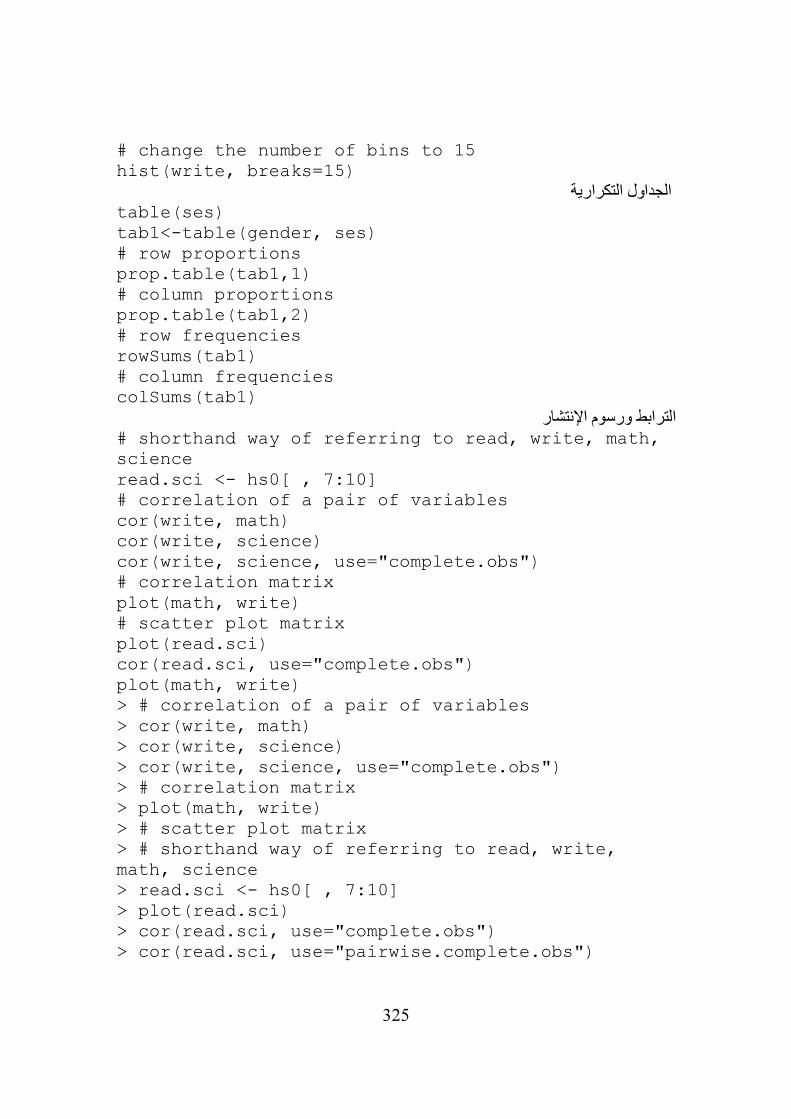
325
# change the number of bins to 15 hist(write, breaks=15)
الجداول التكرارية table(ses) tab1<-table(gender, ses) # row proportions prop.table(tab1,1) # column proportions prop.table(tab1,2) # row frequencies rowSums(tab1) # column frequencies colSums(tab1)
الترابط ورسوم اإلنتشار# shorthand way of referring to read, write, math, science read.sci <- hs0[ , 7:10] # correlation of a pair of variables cor(write, math) cor(write, science) cor(write, science, use="complete.obs") # correlation matrix plot(math, write) # scatter plot matrix plot(read.sci) cor(read.sci, use="complete.obs") plot(math, write) > # correlation of a pair of variables > cor(write, math) > cor(write, science) > cor(write, science, use="complete.obs") > # correlation matrix > plot(math, write) > # scatter plot matrix > # shorthand way of referring to read, write, math, science > read.sci <- hs0[ , 7:10] > plot(read.sci) > cor(read.sci, use="complete.obs") > cor(read.sci, use="pairwise.complete.obs")
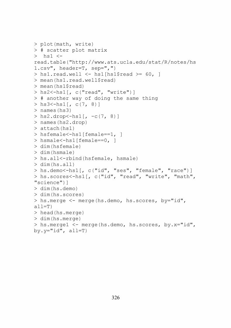
326
> plot(math, write) > # scatter plot matrix > hs1 <- read.table("http://www.ats.ucla.edu/stat/R/notes/hs1.csv", header=T, sep=",") > hs1.read.well <- hs1[hs1$read >= 60, ] > mean(hs1.read.well$read) > mean(hs1$read) > hs2<-hs1[, c("read", "write")] > # another way of doing the same thing > hs3<-hs1[, c(7, 8)] > names(hs3) > hs2.drop<-hs1[, -c(7, 8)] > names(hs2.drop) > attach(hs1) > hsfemale<-hs1[female==1, ] > hsmale<-hs1[female==0, ] > dim(hsfemale) > dim(hsmale) > hs.all<-rbind(hsfemale, hsmale) > dim(hs.all) > hs.demo<-hs1[, c("id", "ses", "female", "race")] > hs.scores<-hs1[, c("id", "read", "write", "math", "science")] > dim(hs.demo) > dim(hs.scores) > hs.merge <- merge(hs.demo, hs.scores, by="id", all=T) > head(hs.merge) > dim(hs.merge) > hs.merge1 <- merge(hs.demo, hs.scores, by.x="id", by.y="id", all=T)
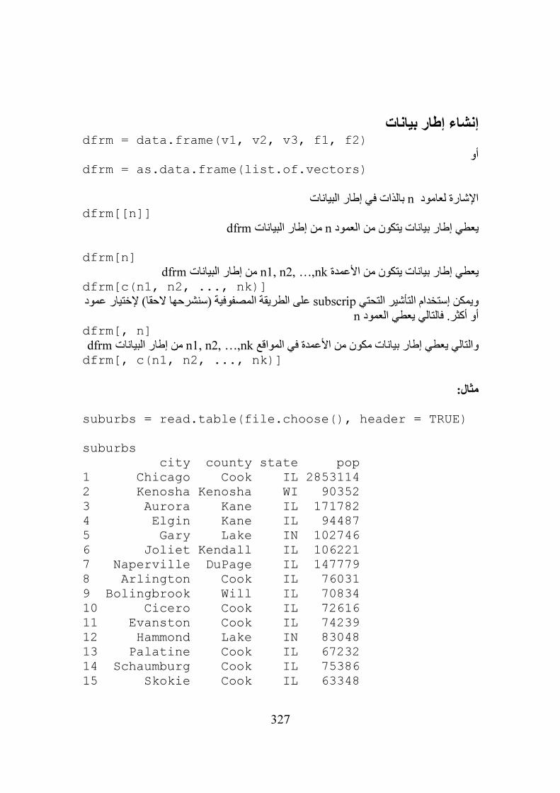
327
إطار بيانات إنشاءdfrm = data.frame(v1, v2, v3, f1, f2)
أوdfrm = as.data.frame(list.of.vectors)
بالذات في إطار البيانات nاإلشارة لعامود
dfrm[[n]] dfrmمن إطار البيانات nعمود يعطي إطار بيانات يتكون من ال
dfrm[n]
dfrmمن إطار البيانات n1, n2, …,nkيعطي إطار بيانات يتكون من األعمدة dfrm[c(n1, n2, ..., nk)]
على الطريقة المصفوفية (سنشرحها الحقا) إلختيار عمود subscripويمكن إستخدام التأشير التحتي nأو أكثر. فالتالي يعطي العمود
dfrm[, n] dfrmمن إطار البيانات n1, n2, …,nkوالتالي يعطي إطار بيانات مكون من األعمدة في المواقع
dfrm[, c(n1, n2, ..., nk)]
مثال:
suburbs = read.table(file.choose(), header = TRUE) suburbs city county state pop 1 Chicago Cook IL 2853114 2 Kenosha Kenosha WI 90352 3 Aurora Kane IL 171782 4 Elgin Kane IL 94487 5 Gary Lake IN 102746 6 Joliet Kendall IL 106221 7 Naperville DuPage IL 147779 8 Arlington Cook IL 76031 9 Bolingbrook Will IL 70834 10 Cicero Cook IL 72616 11 Evanston Cook IL 74239 12 Hammond Lake IN 83048 13 Palatine Cook IL 67232 14 Schaumburg Cook IL 75386 15 Skokie Cook IL 63348
328
16 Waukegan Lake IL 91452 suburbs[[1]] [1] "Chicago" "Kenosha" "Aurora" "Elgin" [5] "Gary" "Joliet" "Naperville" "Arlington Heights" [9] "Bolingbrook" "Cicero" "Evanston" "Hammond" [13] "Palatine" "Schaumburg" "Skokie" "Waukegan" suburbs[1] city 1 Chicago 2 Kenosha 3 Aurora 4 Elgin 5 Gary 6 Joliet 7 Naperville 8 Arlington Heights 9 Bolingbrook 10 Cicero 11 Evanston 12 Hammond 13 Palatine 14 Schaumburg 15 Skokie 16 Waukegan suburbs[c(1,3)] city pop 1 Chicago 2853114 2 Kenosha 90352 3 Aurora 171782 4 Elgin 94487 5 Gary 102746 6 Joliet 106221 7 Naperville 147779 8 Arlington Heights 76031 9 Bolingbrook 70834 10 Cicero 72616
329
11 Evanston 74239 12 Hammond 83048 13 Palatine 67232 14 Schaumburg 75386 15 Skokie 63348 16 Waukegan 91452 suburbs[,1] [1] "Chicago" "Kenosha" "Aurora" "Elgin" [5] "Gary" "Joliet" "Naperville" "Arlington Heights" [9] "Bolingbrook" "Cicero" "Evanston" "Hammond" [13] "Palatine" "Schaumburg" "Skokie" "Waukegan" suburbs[,c(1,4)] city pop 1 Chicago 2853114 2 Kenosha 90352 3 Aurora 171782 4 Elgin 94487 5 Gary 102746 6 Joliet 106221 7 Naperville 147779 8 Arlington Heights 76031 9 Bolingbrook 70834 10 Cicero 72616 11 Evanston 74239 12 Hammond 83048 13 Palatine 67232 14 Schaumburg 75386 15 Skokie 63348 16 Waukegan 91452
:conء إطار بيانات عن طريق إنشاdata = read.table(header=T, con = textConnection(' subject sex size 1 M 7 2 F 6 3 F 9 4 M 11 '))
330
close(con) data subject sex size 1 1 M 7 2 2 F 6 3 3 F 9 4 4 M 11
:Negative Indexing التأشير السلبيx = c(1,4,4,3,2,2,3) x [1] 1 4 4 3 2 2 3 x[-1] [1] 4 4 3 2 2 3
يعطي المتجه بدون العنصر األول.x[-1:-3] [1] 3 2 2 3
3إلى 1يعطي المتجه بدون العناصر من x[-length(x)] [1] 1 4 4 3 2 2
ي المتجه بدون العنصر األخير.يعط
الدوال المفيدة: بعض rep) الدالة 1
y = rep(1, 10) y [1] 1 1 1 1 1 1 1 1 1 1 z = rep(1:5, 4) z [1] 1 2 3 4 5 1 2 3 4 5 1 2 3 4 5 1 2 3 4 5 w = rep(1:5, each=4) w [1] 1 1 1 1 2 2 2 2 3 3 3 3 4 4 4 4 5 5 5 5 abc = rep(factor(LETTERS[1:3]), 5)
331
abc [1] A B C A B C A B C A B C A B C Levels: A B C
lsالدالة )2ls() [1] "abc" "con" "data" "df" "let" "n" "suburbs" "v" "w" "x" [11] "y" "z"
لمسح أو إزالة متجه rm) الدالة 3rm(v) ls() [1] "abc" "con" "data" "df" "let" "n" "suburbs" "w" "x" "y" [11] "z"
) دالة إيجاد حجم (طول) متجه4length(x) [1] 1 length(y) [1] 10 length(n) [1] 4
متجه أو مصفوفة ) عدد األسطر وعدد األعمدة في إطار بيانات أو5nrow(df) [1] 4 ncol(df) [1] 2 dim(df) [1] 4 2
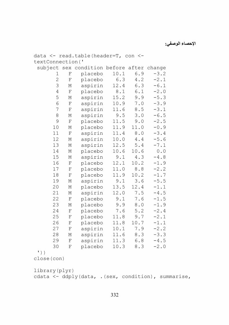
332
اإلحصاء الوصفي:
data <- read.table(header=T, con <- textConnection(' subject sex condition before after change 1 F placebo 10.1 6.9 -3.2 2 F placebo 6.3 4.2 -2.1 3 M aspirin 12.4 6.3 -6.1 4 F placebo 8.1 6.1 -2.0 5 M aspirin 15.2 9.9 -5.3 6 F aspirin 10.9 7.0 -3.9 7 F aspirin 11.6 8.5 -3.1 8 M aspirin 9.5 3.0 -6.5 9 F placebo 11.5 9.0 -2.5 10 M placebo 11.9 11.0 -0.9 11 F aspirin 11.4 8.0 -3.4 12 M aspirin 10.0 4.4 -5.6 13 M aspirin 12.5 5.4 -7.1 14 M placebo 10.6 10.6 0.0 15 M aspirin 9.1 4.3 -4.8 16 F placebo 12.1 10.2 -1.9 17 F placebo 11.0 8.8 -2.2 18 F placebo 11.9 10.2 -1.7 19 M aspirin 9.1 3.6 -5.5 20 M placebo 13.5 12.4 -1.1 21 M aspirin 12.0 7.5 -4.5 22 F placebo 9.1 7.6 -1.5 23 M placebo 9.9 8.0 -1.9 24 F placebo 7.6 5.2 -2.4 25 F placebo 11.8 9.7 -2.1 26 F placebo 11.8 10.7 -1.1 27 F aspirin 10.1 7.9 -2.2 28 M aspirin 11.6 8.3 -3.3 29 F aspirin 11.3 6.8 -4.5 30 F placebo 10.3 8.3 -2.0 ')) close(con)
library(plyr) cdata <- ddply(data, .(sex, condition), summarise,

333
N = length(change), change = mean(change), sd = sd(change), se = sd(change) / sqrt(length(change)) )
dataNA <- data dataNA$change[11:14] <- NA cdata <- ddply(dataNA, .(sex, condition), summarise, N = sum(!is.na(change)), change = mean(change, na.rm=TRUE), sd = sd(change, na.rm=TRUE), se = sd(change, na.rm=TRUE) / sqrt(sum(!is.na(change))) )
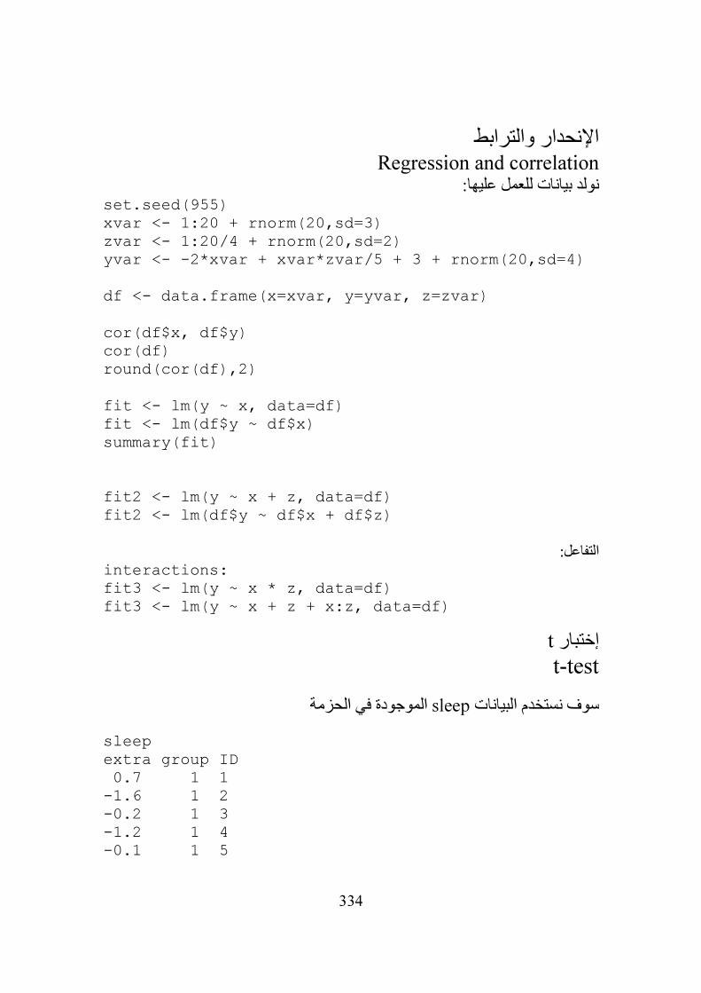
334
دار والترابطاإلنحRegression and correlation
نولد بيانات للعمل عليها:set.seed(955) xvar <- 1:20 + rnorm(20,sd=3) zvar <- 1:20/4 + rnorm(20,sd=2) yvar <- -2*xvar + xvar*zvar/5 + 3 + rnorm(20,sd=4) df <- data.frame(x=xvar, y=yvar, z=zvar) cor(df$x, df$y) cor(df) round(cor(df),2) fit <- lm(y ~ x, data=df) fit <- lm(df$y ~ df$x) summary(fit) fit2 <- lm(y ~ x + z, data=df) fit2 <- lm(df$y ~ df$x + df$z)
التفاعل:interactions: fit3 <- lm(y ~ x * z, data=df) fit3 <- lm(y ~ x + z + x:z, data=df)
tإختبار
t-test
الموجودة في الحزمة sleepسوف نستخدم البيانات
sleep extra group ID 0.7 1 1 -1.6 1 2 -0.2 1 3 -1.2 1 4 -0.1 1 5
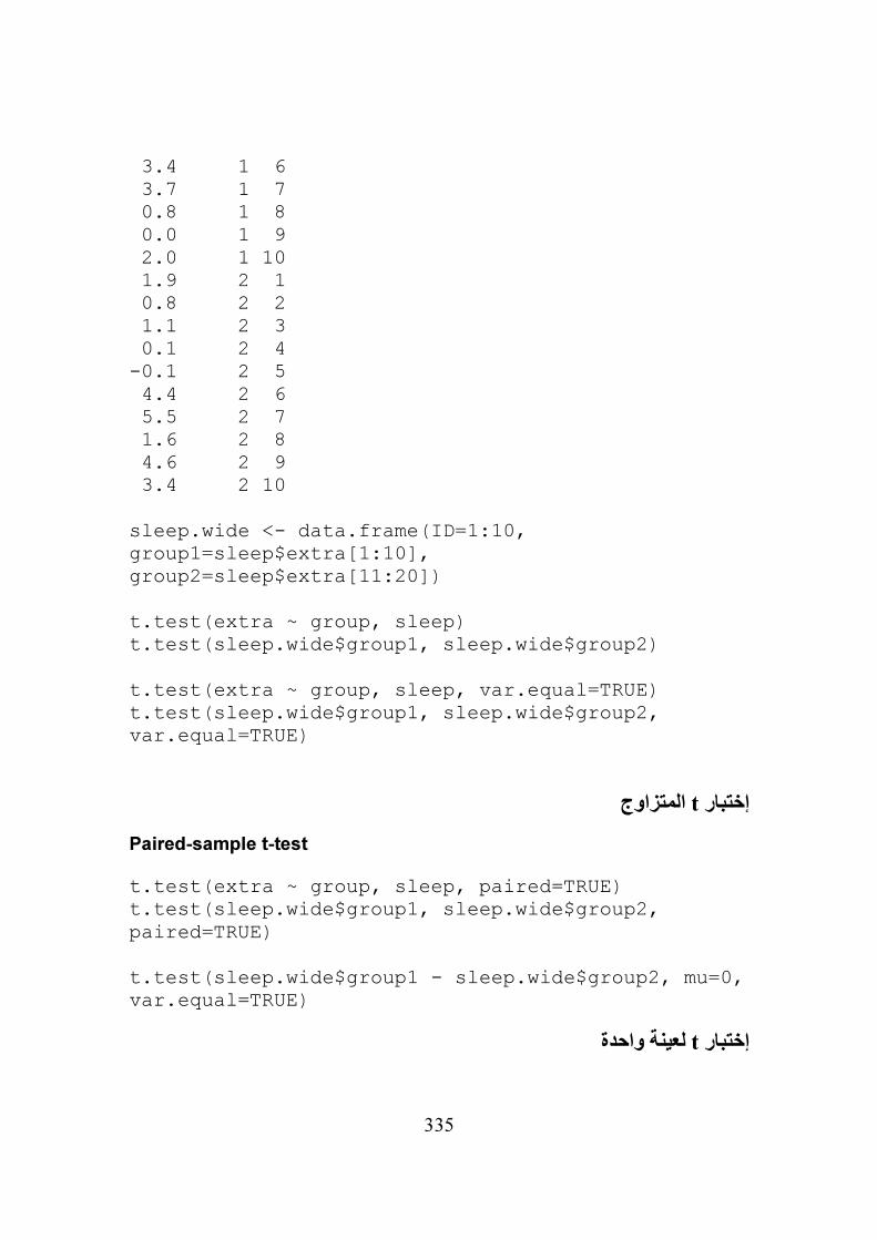
335
3.4 1 6 3.7 1 7 0.8 1 8 0.0 1 9 2.0 1 10 1.9 2 1 0.8 2 2 1.1 2 3 0.1 2 4 -0.1 2 5 4.4 2 6 5.5 2 7 1.6 2 8 4.6 2 9 3.4 2 10 sleep.wide <- data.frame(ID=1:10, group1=sleep$extra[1:10], group2=sleep$extra[11:20]) t.test(extra ~ group, sleep) t.test(sleep.wide$group1, sleep.wide$group2) t.test(extra ~ group, sleep, var.equal=TRUE) t.test(sleep.wide$group1, sleep.wide$group2, var.equal=TRUE)
المتزاوج tإختبار
Paired-sample t-test
t.test(extra ~ group, sleep, paired=TRUE) t.test(sleep.wide$group1, sleep.wide$group2, paired=TRUE) t.test(sleep.wide$group1 - sleep.wide$group2, mu=0, var.equal=TRUE)
لعينة واحدة tإختبار
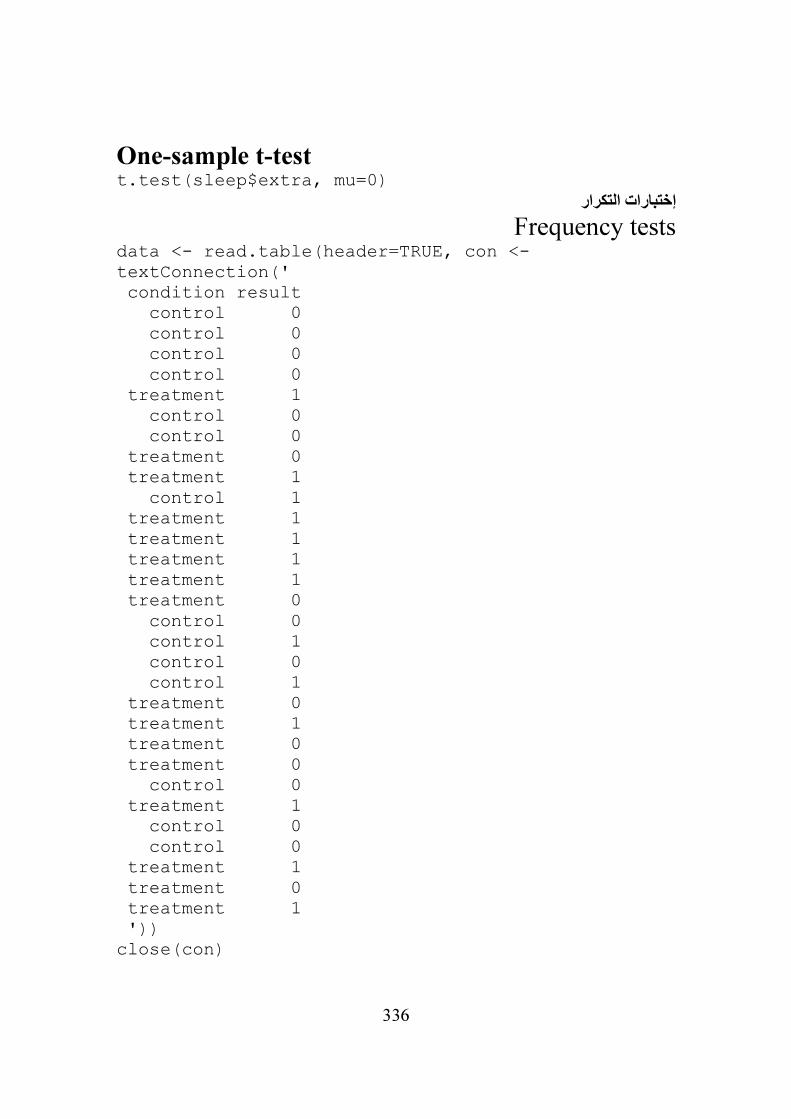
336
One-sample t-test t.test(sleep$extra, mu=0)
إختبارات التكرار
Frequency tests data <- read.table(header=TRUE, con <- textConnection(' condition result control 0 control 0 control 0 control 0 treatment 1 control 0 control 0 treatment 0 treatment 1 control 1 treatment 1 treatment 1 treatment 1 treatment 1 treatment 0 control 0 control 1 control 0 control 1 treatment 0 treatment 1 treatment 0 treatment 0 control 0 treatment 1 control 0 control 0 treatment 1 treatment 0 treatment 1 ')) close(con)
337
إختبارات حسن المطابقةTests of goodness-of-fit
إختبار مربع كاي
Chi-square test ct <- table(data$result) # An alternative is to manually create the table #ct <- matrix(c(17,13), ncol=2) #colnames(ct1) <- c("0", "1") chisq.test(ct) ct <- table(data$result) pt <- c(.75, .25) chisq.test(ct, p=pt)
إختبارات اإلستقاللTests of independence
إختبار مربع كاي
Chi-square test ct <- table(data$condition, data$result) chisq.test(ct) chisq.test(ct, correct=FALSE)
338
تحليل التباينANOVA
data <- read.table(header=T, con <- textConnection(' subject sex age before after 1 F old 9.5 7.1 2 M old 10.3 11.0 3 M old 7.5 5.8 4 F old 12.4 8.8 5 M old 10.2 8.6 6 M old 11.0 8.0 7 M young 9.1 3.0 8 F young 7.9 5.2 9 F old 6.6 3.4 10 M young 7.7 4.0 11 M young 9.4 5.3 12 M old 11.6 11.3 13 M young 9.9 4.6 14 F young 8.6 6.4 15 F young 14.3 13.5 16 F old 9.2 4.7 17 M young 9.8 5.1 18 F old 9.9 7.3 19 F young 13.0 9.5 20 M young 10.2 5.4 21 M young 9.0 3.7 22 F young 7.9 6.2 23 M old 10.1 10.0 24 M young 9.0 1.7 25 M young 8.6 2.9 26 M young 9.4 3.2 27 M young 9.7 4.7 28 M young 9.3 4.9 29 F young 10.7 9.8 30 M old 9.3 9.4 ')) close(con)

339
تحليل التباين في إتجاه واحد بين المعالجات
One way between ANOVA
# One way between: # IV: sex # DV: before aov.before.sex <- aov(before ~ sex, data=data) summary(aov.before.sex)
تحليل التباين في إتجاهين بين المعالجات
Two way between ANOVA
# 2x2 between: # IV: sex # IV: age # DV: after # These two calls are equivalent aov.after.sex.age <- aov(after ~ sex*age, data=data) aov.after.sex.age <- aov(after ~ sex + age + sex:age, data=data) summary(aov.after.sex.age)
أمثلة: نات ومتغيرات جديدة نقوم بإزالة المتغيرات الحاليةقبل العمل على بيا
rm(list=ls())
ندخل البيانات الجديدة ونفعلها
hs1 <- read.table("http://www.ats.ucla.edu/stat/R/notes/hs1.csv", header=T, sep=",") attach(hs1)
إختبار مربع كاي لإلستقاللtab1 <- table(female, ses) # chi-square test of independence summary(tab1)
لعينة واحدة tإختبار t.test(write, mu=50)
المتزاوج tإختبار t.test(write, read, paired=TRUE)

340
tالتباين إلختبار فحص by(write, female, var) tapply(write, female, var) # assuming equal variances t.test(write~female, var.equal=TRUE) # assuming unequal variances t.test(write~female, var.equal=FALSE)
تحليل التباين:
anova(lm(write~factor(prog))) summary(aov(write~factor(prog)))
m2<-lm(write~factor(prog)*factor(female)) anova(m2) anova(lm(write~factor(prog) + read)) summary(aov(write~factor(prog) + read))
تحليل اإلنحدار:
summary(lm(write~female+read)) lm2 <- lm(write~read+socst) summary(lm2) # plotting diagnostic plots of lm2 plot(lm2) write[1:20] fitted(lm2)[1:20] resid(lm2)[1:20]

341
Numerical Methods طرق عددية: شتقات العدديةالم
Numerical Derivatives Examples library(mosaic) g = numD( a*x^2 + x*y ~ x, a=1) g(x=2,y=10) gg = numD( a*x^2 + x*y ~ x&x, a=1) gg(x=2,y=10) ggg = numD( a*x^2 + x*y ~ x&y, a=1) ggg(x=2,y=10) h = numD( g(x=x,y=y,a=a) ~ y, a=1) h(x=2,y=10) f = numD( sin(x)~x, add.h.control=TRUE) plotFun( f(3,.hstep=h)~h, hlim=range(.00000001,.000001)) ladd( panel.abline(cos(3),0))
R Summary Examples ===========Getting Help in R========== ?read.table find(lowess) apropos(lm) ============Worked Examples of Functions=== example(lm) =========Demonstrations of R Functions========= demo(persp) demo(graphics) demo(Hershey) demo(plotmath) ==================Libraries in R============= library(spatial) ===============Contents of Libraries======= library(help=spatial) objects(grep("spatial",search())) =======Installing Packages and Libraries========= install.packages("akima") install.packages("chron") install.packages("Ime4")

342
install.packages("mcmc") install.packages("odesolve") install.packages("spdep") install.packages("spatstat") install.packages("tree") ===================Data Editor================= library(MASS) attach(bacteria) fix(bacteria) ==================Significance Stars============ options(show.signif.stars=FALSE) options( digits = 3) ========To stop multiple graphs whizzing by==== par(ask=TRUE) ================Good Housekeeping============ objects() search() ls() rm(list=ls()) rm(x,y,z) detach(worms) ====Summary Information from Vectors by Groups===== data<-read.table("c:\\temp\\daphnia.txt",header=T) attach(data) names(data) tapply(Growth.rate,Detergent,mean) tapply(Growth.rate,list(Water,Daphnia),median) with(data, function( ...)) with(OrchardSprays,boxplot(decrease~treatment)) library(MASS) with(bacteria,tapply((y=="n"),trt,sum)) with(mammals,plot(body,brain,log="xy")) reg.data<-read.table("c:\\temp\\regression.txt",header=T) with (reg.data, { model<-lm(growth~tannin) summary(model) } ) summary(lm(growth~tannin,data=reg.data)) =======To see the names of the dataframes in the built-in package called datasets==== data()

343
==========To see all available data sets========= data(package = .packages(all.available = TRUE)) =============Sorting, Ranking and Ordering======= houses<-read.table("c:\\temp \\houses.txt",header=T) attach(houses) names(houses) [1] "Location" "Price" ranks<-rank(Price) sorted<-sort(Price) ordered<-order(Price) view<-data.frame(Price,ranks,sorted,ordered) view ===============Matrices======================== X<-matrix(c(1,0,0,0,1,0,0,0,1),nrow=3) X vector<-c(1,2,3,4,4,3,2,1) V<-matrix(vector,byrow=T,nrow=2) V ====================Data Input============== y <- c (6,7,3,4,8,5,6,2) x<-scan() (enter data, to finish return) ===============Data Input from Files=========== data<-read.table("c:\\temp\\regression.txt",header=T) map<-read.table("c:\\temp\\bowens.csv",header=T,sep=",") map<-read.csv("c:\\temp\\bowens.csv") read.delim("c:\\temp\\file.txt") ===============Browsing to Find Files========== data<-read.table(file.choose(),header=T) =============Reading from clipboard========= data <-read.table("clipboard", sep = " ")) ==============Setting the Working Directory=====

344
setwd("c:\\temp") getwd() =====================Dataframes=============== worms<-read.table(file.choose(), header = T) attach(worms) names(worms) summary(worms) by(worms,Vegetation,mean) ===============Subscripts and Indices========= worms[3,5] worms[14:19,7] worms[1:5,2:3] worms[3,] worms[,3] worms[,c(1,5)] ===================Sorting Dataframes=========== worms[order(Slope),] worms[rev(order(Slope)),] worms[order(Vegetation,Worm.density),] ====Omitting Rows Containing Missing Values, NA==== na.omit(data) new.frame<-na.exclude(data) ===Dataframe with Row Names instead of Row Numbers= worms<-read.table(file.choose(),header=T,row.names=1) ====Summarizing the Contents of Dataframes ======= aggregate(worms[,c(2,3,5,7)],by=list(veg=Vegetation),mean) aggregate(worms[,c(2,3,5,7)],by=list(veg=Vegetation,d=Damp),mean) ========Adding Normal Curve to histogram======== x<-rnorm(300) h<-hist(x, breaks=10, col="red", xlab="Simulated Data", main="Histogram with Normal Curve") xfit<-seq(min(x),max(x),length=40) yfit<-dnorm(xfit,mean=mean(x),sd=sd(x)) yfit <- yfit*diff(h$mids[1:2])*length(x) lines(xfit, yfit, col="blue", lwd=2) ====another example========= n <- 1000 x <- rnorm(n) h <- hist(x, col="red",freq=TRUE)

345
dx <- min(diff(h$breaks)) curve(n*dx*dnorm(x), add=TRUE, col="blue", lwd=2) ===Classical Tests===Plots for testing normality == x<-exp(rnorm(30)) qqnorm(x) qqline(x,lty=2) ================Test for normality=============== x<-exp(rnorm(30)) shapiro.test(x) wilcox.test(x,mu=0) hist(x) skew(x) kurtosis(x) ==========quantiles of the F distribution========= qf(0.975,9,9) ======F test to compare two variances======== x<-exp(rnorm(30)) y<-exp(rnorm(30)) var.test(x,y) ====Bartlett test of homogeneity of variances ===== bartlett.test(x,y) ===Comparing two means==Student’s t test====== qt(0.975,18) t.test(x,y) ==================Tests on paired samples========= t.test(x,y,paired=T) =======Chi-squared contingency tables======== qchisq(0.95,1) count<-matrix(c(38,14,11,51),nrow=2) chisq.test(count) chisq.test(count,correct=F) chisq.test(count,correct=F)$expected ============Test of contingency========= chisq.test(c(10,3,2,6)) chisq.test(c(10,3,2,6),p=c(0.2,0.2,0.3,0.3)) die<-ceiling(runif(100,0,6))

346
table(die) chisq.test(table(die)) =======Fisher’s Exact Test for Count Data ====== x<-as.matrix(c(6,4,2,8)) dim(x)<-c(2,2) fisher.test(x) =========Correlation and covariance============= var(x,y) ====covariance of x and y=== cor(x,y) =====Pearson’s product-moment correlation======== cor.test(Summer, Winter) cor.test(x,y,method="spearman") =============Kolmogorov–Smirnov test============ ks.test(A,B) =========Regression====very simple intro=== reg<-lm(y ~ x) summary(reg) lm.influence(lm(growth~tannin)) influence.measures(lm(growth ~ tannin)) model<-lm(Fruit ~ Root,subset=(Grazing=="Grazed")) ==== na.action = na.omit model<-lm(Fruit ~ Grazing*Root,na.action=na.fail) AIC(model) model.1<-lm(Fruit ~ Grazing*Root) model.2<-lm(Fruit ~ Grazing+Root) AIC(model.1, model.2) ==================Leverage=========== leverage(x1) plot(leverage(x1),type="h") abline(0.66,0,lty=2) points(leverage(x1)) ======Extracting components of the model using $ == model$coef model$fitted model$resid model$df ==Extracting components from the summary.aov table= summary.aov(model) summary.aov(model)

347
Df Sum Sq Mean Sq F value Pr(>F) tannin 1 88.817 88.817 30.974 0.000846 Residuals 7 20.072 2.867 summary.aov(model)[[1]][[1]] [1] 1 7 summary.aov(model)[[1]][[2]] [1] 88.81667 20.07222 summary.aov(model)[[1]][[3]] [1] 88.816667 2.867460 summary.aov(model)[[1]][[4]] [1] 30.97398 NA summary.aov(model)[[1]][[5]] [1] 0.0008460738 NA model<-lm(biomass ~ clipping) summary.aov(model) summary.lm(model) anova(model6,model7) ===========Prediction using the fitted model== model<-lm(growth~tannin) predict(model,list(tannin=5.5)) predict(model,list(tannin=c(3.3,4.4,5.5,6.6))) ===============Model checking======== par(mfrow=c(2,2)) plot(model) ==========The Multiple Regression Model========= model7<-lm(log(ozone) ~ temp + wind + rad + I(temp^2) + I(wind^2)) summary(model7) ===================Step reg======= model10<-step(model1) summary(model10) pairs(pollute,panel=panel.smooth) ================One-Way ANOVA======== results<-read.table("c:\\temp\\yields.txt",header=T) attach(results)

348
names(results) sapply(list(sand,clay,loam),mean) y<-c(sand,clay,loam) soil<-factor(rep(1:3,c(10,10,10))) sapply(list(sand,clay,loam),var) plot(soil,y,names=c("sand","clay","loam"),ylab="yield") summary(aov(y~soil)) plot(aov(y~soil)) summary.lm(aov(y~soil)) summary.lm(model1) summary.aov(model2) > x<-rnorm(150) > h<-hist(x,breaks=15) > xhist<-c(min(h$breaks),h$breaks) > yhist<-c(0,h$density,0) > xfit<-seq(min(x),max(x),length=40) > yfit<-dnorm(xfit,mean=mean(x),sd=sd(x)) > plot(xhist,yhist,type="s",ylim=c(0,max(yhist,yfit))) > lines(xfit,yfit) > curve(dnorm(x,0,1),xlim=c(-3.5,3.5)) curve(dnorm(x,0,1),-3.5,3.5) > dat <- rnorm(30, mean = 82, sd = 7) > hist(dat, prob = TRUE) > curve(dnorm(x, mean = mean(dat), sd = sd(dat)), add = TRUE) > # Why not throw a kernel density estimate on there too > lines(density(dat), col = "red") > > library(descr) Warning message: package ‘descr’ was built under R version 2.15.1 > dat <- rnorm(30, mean = 82, sd = 7) > histkdnc(dat) > dat <- rnorm(3000, mean = 82, sd = 7) > histkdnc(dat) > x <- rnorm(1000) hist(x, freq = FALSE, col = "grey") curve(dnorm, col = 2, add = TRUE)
349
Glossary • Basic arithmetic operators: ( ) brackets in arithmetic calculations
^ raise to the power of / division * multiplication + addition - subtraction
• Assignment operator <- assigns the value of the expression on the right to the identifer on the left. • Concatenation function c(...) argument is a set of values; returns a vector
containing those values. • Simple statistical functions sum(...)
mean(...)
median(...)
range(...) sd(...) standard deviation mad(...) mean absolute deviation IQR(...) inter-quartile range min(...) minimum max(...) maximum
• Help ? ... will provide information on function usage and arguments help.start() opens html help files • Session management objects() lists objects in workspace
ls() does the same as objects() rm(...) removes the objects listed from workspace rm(list = objects()) removes all objects from workspace getwd() returns the current working directory setwd(...) set the working directory dir() list files in current directory save.image(...) saves workspace to specified file quit() ends R session load(...) loads a saved workspace from file
• Load data from text file read.table(...) argument is a file in the working directory. Return value is a data frame. • Editing data fix(...) or data.entry(...) brings up spreadsheet like environment for editing data. • Scatterplot plot(...) is a versatile plotting command, draws a scatterplot when two arguments are given. • Linear model fitting lm(...) can fit a variety of linear models, argument is a model formula. • Basic inference t.test(...) Student's t-test
var.test(...) F test to compare two variances
chisq.test(...) Pearson's 2
χ test for count data
350
cor.test(...) test for association • Object properties length(...)
mode(...)
typeof(...)
class(...)
attributes(...) returns all non-intrinsic attributes • Object contents summary(...) information on an object; output depends on class
str(...) compact details of object structure dput(...) text listing of object
• Regular sequences : sequence generator gives sequence with unit steps
between left and right arguments seq(...) more general regular sequence generator,
can set step (by) and/or length of sequence (length) rep(...) for generating sequence with repeated values
• Logical values TRUE and FALSE • Comparison and logical operators == equality != inequality < less than > greater than <= less than or equal to >= greater than or equal to ! negation & and (&& scalar version)
| or (|| scalar version)
• Accessing elements [...] contents of brackets a vector of integers, a vector of logical values or a vector of names.
• Accessing a list component [[...]] contents of brackets a number or a name. • Accessing a named component $ • Referring to list components directly attach(...) brings components of a list into view; use detach() to tidy up. • Generating a vector of strings paste(...) converts any non-character arguments into characters and puts them together into a vector of mode character.
• Generating lists list(...) put arguments (which may be named) into a list. • A selection of plots hist(...) histogram
qqnorm(...) normal qq-plot boxplot(...) contour(...) 3D contours image(...) 3D coloured blocks persp(...) 3D wire frame
• Some low level plotting commands points(...) lines(...) text(...)

351
• Some graphics parameters pch plotting character col colour mfrow multi-figure page specification mfcol
• Storing commands savehistory(...)
loadhistory(...)
source(...)
• Packages library(...) list and load packages
data(...) add data from a package to workspace
• Search path search() lists environments in the search path in
the order in which
theywill be searched. Passing the
position in search path
or name of an environments
to objects(...) lists objects
in that environment.
• Arrays matrix(...) to generate a matrix (2D array)
array(...) to generate a general array.

352
تبارات السابقةأسئلة وإجابات اإلخ
353
بسم هللا الرحمن الرحيم
جامعة الملك سعود قسم اإلحصاء وبحوث العمليات
بحث (طرق الحسابات في بحوث العمليات ) 433مادة هـ 1423/1424اإلختبار النهائي للفصل األول
ساعات 3الزمن
أجب على سؤالين من األسئلة التالية:
التالي: أجب EXCELالسؤال األول: بإستخدام
)أ) بتقريب المشتقتين األولى و الثانية بثالثة نقاط أوجد عدديا المشتقتين األولى و الثانية للدالة ) ( )sinxf x e x=
0xعند 0.01hو = =.
)ب) قرب الدالة ) ( )f x n x= ℓ قطة بكثيرة حدود حول الن0
1x =.
ج) بإستخدام المحاكاة أوجد التكامل العددي للتالي:
( )0
sin x dxπ
∫
.2القيمة الحقيقية هي د) حل المعادلة التفاضلية التالية:
( ), 0 0dx
tx t xdt
+ = =
]في الفترة ]0,1 .
حل التالي: EXCEL SOLVERام السؤال الثاني: بإستخد
1 2 3 4 5 6
1 2 3 4 5 6
1 2 3 4 5 6
1 2 3 4 5 6
1 2
1 8 10 7 6 11 9
12 9 25 20 17 13 60
35 42 18 31 56 49 150
37 53 28 24 29 20 125
0 , 1
Minimize x x x x x x
Subject to
x x x x x x
x x x x x x
x x x x x x
x x
− + + + + +
+ + + + + ≥
+ + + + + ≥
+ + + + + ≥
≤ ≤
حل المشكلة التالية: LINGOالسؤال الثالث: بإستخدام لغة البرمجة الرياضية لألمثلية مع توضيح المجوعات والبيانات والمتغيرات والهدف والقيود.
و Pawnبعة تعرف بأألسماء التجارية أصناف من المكسرات المشكلة. األصناف األر 4شركة تصنيع حلويات تسوق Knight وBishop وKing كل صنف يحتوي على نسبة محددة من اللوز . Peanuts و الكاشوCashews .
الجدول التالي يعطي عدد االونسات من اللوز والكاشو في كل رطل من األصناف األربعة وسعربيع الرطل لكل صنف:
Pawn Knight Bishop King
Peanuts (oz.) 15 10 6 2 Cashews (oz.) 1 6 10 14
Selling Price ($) 2 3 4 5

354
رطل من الكاشو يوميا ألغراض اإلنتاج. مشكلة 250رطل من اللوز و 750أبرمت الشركة عقد مع جهة لتموينها تجاوز الكميات الشركة هي تحديد عدد األرطال التي تنتجها كل يوم من كل صنف بحيث تحقق أقصى دخل بدون
الموردة يوميا من اللوز والكاشو.

355
بعض الصيغ المساعدة: تقريب المشتقات عدديا:
تقريب المشتقة األولى بثالثة نقاط
( )( ) ( )
( )22
f x h f x hf x O h
h
+ − −′ = +
تقريب المشتقة الثانية بثالثة نقاط
( )( ) ( ) ( )
( )22
2f x h f x f x hf x O h
h
+ − + −′′ = +
تقرب الدوال بكثيرة حدود:
)تقرب أي دالة )f x ) والتي تكون جميع مشتقاتها موجودة ومعرفة حتى المشتقة النونيةn بكثيرة حدود (
( )1np x
−
كالتالي:
( )( ) ( )
( )1
0
1 0
0 !
kn
k
n
k
f xp x x x
k
−
−
=
= −∑
كالتالي: والتي تسمى بكثيرات حدود تايلور. العالقة السابقة يمكن حسابها تكراريا
( ) ( )( )
( )1 0
!
jj
j j
fp x p x x x
j−
= + −
حل المعادلة التفاضلية العادية: Euler’s Formulaصيغة أويلر
( )1
2 1
1 2
,
,2 2
j j
j j
j j
k f x y
h hk f x y k
y y h k+
=
= + +
= +
إيجاد تكامل بالمحكاة:
تستخدم المحاكاة (أو مايسمى بطريقة مونت كارلو) إليجاد تكامالت من الشكل:
( )b
a
I f x dx= ∫
ب بالمجموعوالتي تقر
( )( )
1
N
i
i
b aI f x
N=
−
≈ ∑
وذلك بإختيار ix 1بطريقة عشوائية بدال من إختيارها عند نقاط محددة. الخطأ هو من درجة N وهو عشوائي
تماما واليعتمد على درجة التكامل (أبعاد التكامل).
356
مبسم هللا الرحمن الرحي قسم اإلحصاء وبحوث العمليات
جامعة الملك سعود هـ 1423/1424إختبار فصلي أول للفصل الصيفي
بحث ( طرق الحسابات في بحوث العمليات) 433المادة ساعة: أجب على جميع األسئلة التالية: 2الزمن
السؤال األول:
لنموذج صفحة النشر التالي :
على شكل رياضي. أ) أكتب نموذج صفحة النشر ب) أشرح عمل النموذج.
التالية Solverج) املئ الفراغات في نوافذ
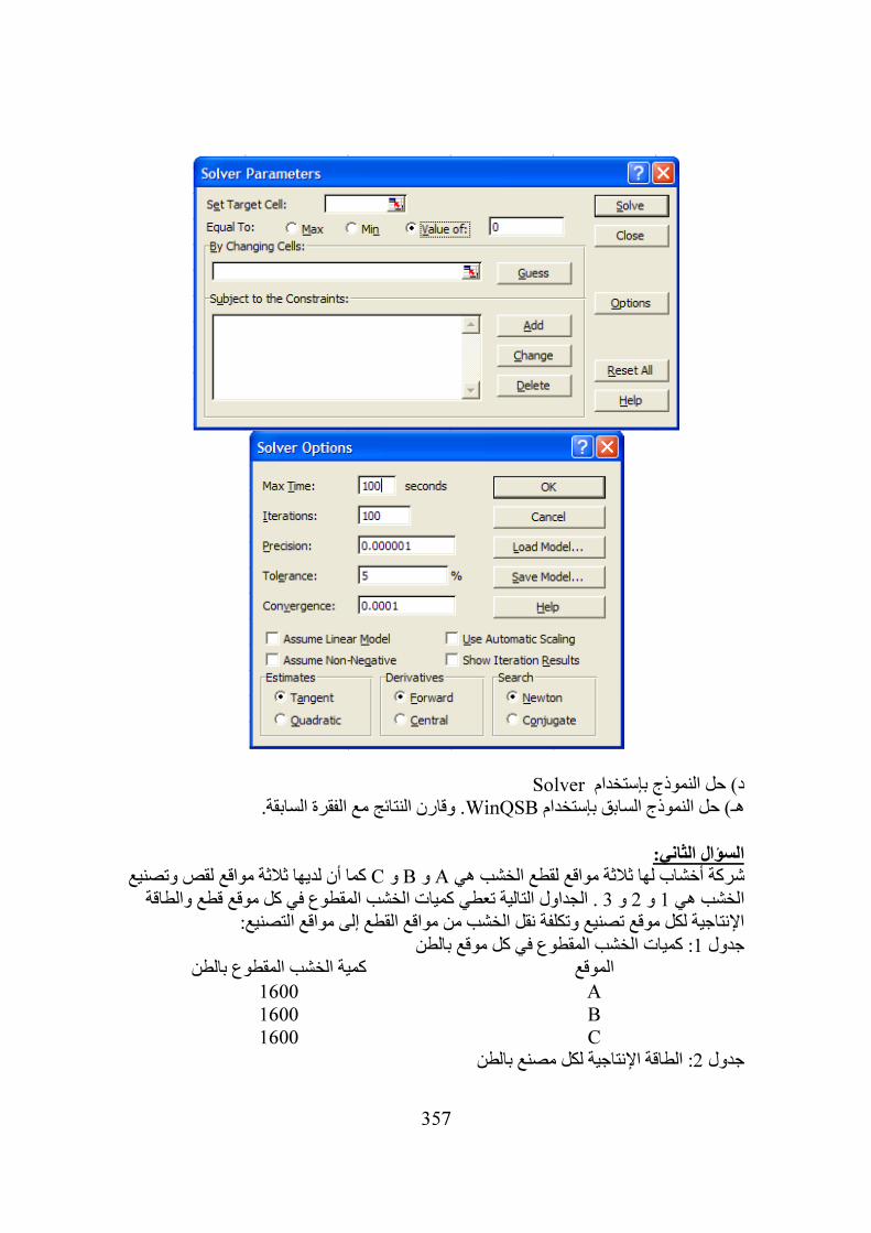
357
Solverد) حل النموذج بإستخدام . وقارن النتائج مع الفقرة السابقة.WinQSBهـ) حل النموذج السابق بإستخدام
السؤال الثاني:
ا أن لديها ثالثة مواقع لقص وتصنيع كم Cو Bو Aشركة أخشاب لها ثالثة مواقع لقطع الخشب هي . الجداول التالية تعطي كميات الخشب المقطوع في كل موقع قطع والطاقة 3و 2و 1الخشب هي
اإلنتاجية لكل موقع تصنيع وتكلفة نقل الخشب من مواقع القطع إلى مواقع التصنيع: : كميات الخشب المقطوع في كل موقع بالطن1جدول
ب المقطوع بالطنكمية الخش الموقعA 1600 B 1600 C 1600
: الطاقة اإلنتاجية لكل مصنع بالطن2جدول
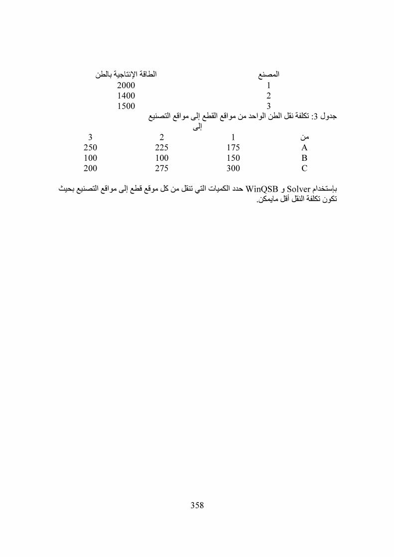
358
الطاقة اإلنتاجية بالطن المصنع1 2000 2 1400 3 1500
: تكلفة نقل الطن الواحد من مواقع القطع إلى مواقع التصنيع3جدول إلى
3 2 1 منA 175 225 250 B 150 100 100 C 300 275 200
حدد الكميات التي تنقل من كل موقع قطع إلى مواقع التصنيع بحيث WinQSBو Solverبإستخدام
تكون تكلفة النقل أقل مايمكن.
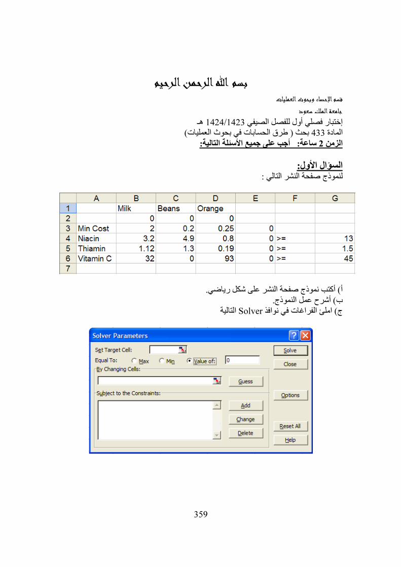
359
بسم هللا الرحمن الرحيم قسم اإلحصاء وبحوث العمليات
جامعة الملك سعود هـ 1423/1424إختبار فصلي أول للفصل الصيفي
سابات في بحوث العمليات) بحث ( طرق الح 433المادة ساعة: أجب على جميع األسئلة التالية: 2الزمن
السؤال األول:
لنموذج صفحة النشر التالي :
أ) أكتب نموذج صفحة النشر على شكل رياضي. ب) أشرح عمل النموذج.
التالية Solverج) املئ الفراغات في نوافذ
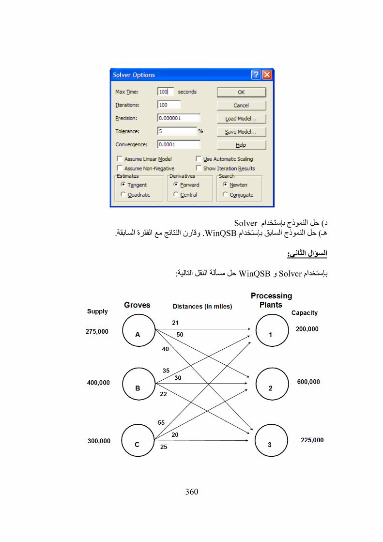
360
Solverد) حل النموذج بإستخدام . وقارن النتائج مع الفقرة السابقة.WinQSBهـ) حل النموذج السابق بإستخدام
السؤال الثاني:
حل مسألة النقل التالية: WinQSBو Solverبإستخدام
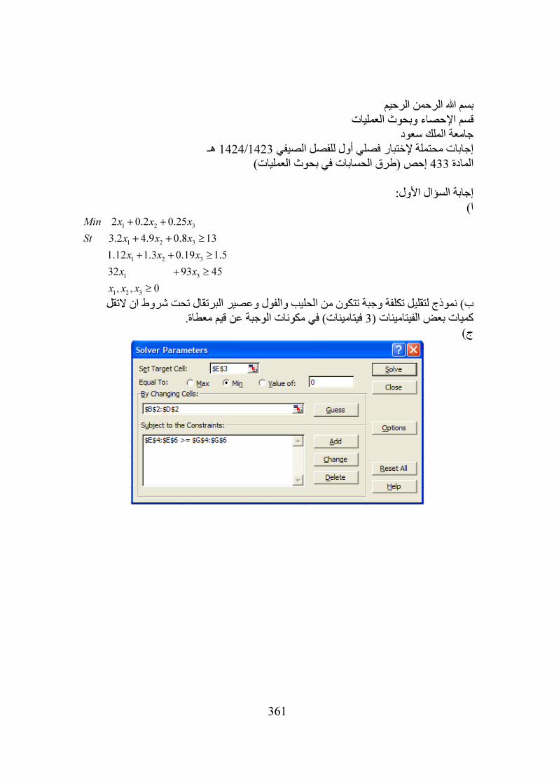
361
بسم هللا الرحمن الرحيم قسم اإلحصاء وبحوث العمليات
جامعة الملك سعود هـ 1423/1424إجابات محتملة إلختبار فصلي أول للفصل الصيفي
إحص (طرق الحسابات في بحوث العمليات) 433المادة
إجابة السؤال األول: ا)
1 2 3
1 2 3
1 2 3
1 3
1 2 3
2 0.2 0.25
3.2 4.9 0.8 13
1.12 1.3 0.19 1.5
32 93 45
, , 0
Min x x x
St x x x
x x x
x x
x x x
+ +
+ + ≥
+ + ≥
+ ≥
≥
ب) نموذج لتقليل تكلفة وجبة تتكون من الحليب والفول وعصير البرتقال تحت شروط ان التقل عطاة.فيتامينات) في مكونات الوجبة عن قيم م 3كميات بعض الفيتامينات (
ج)
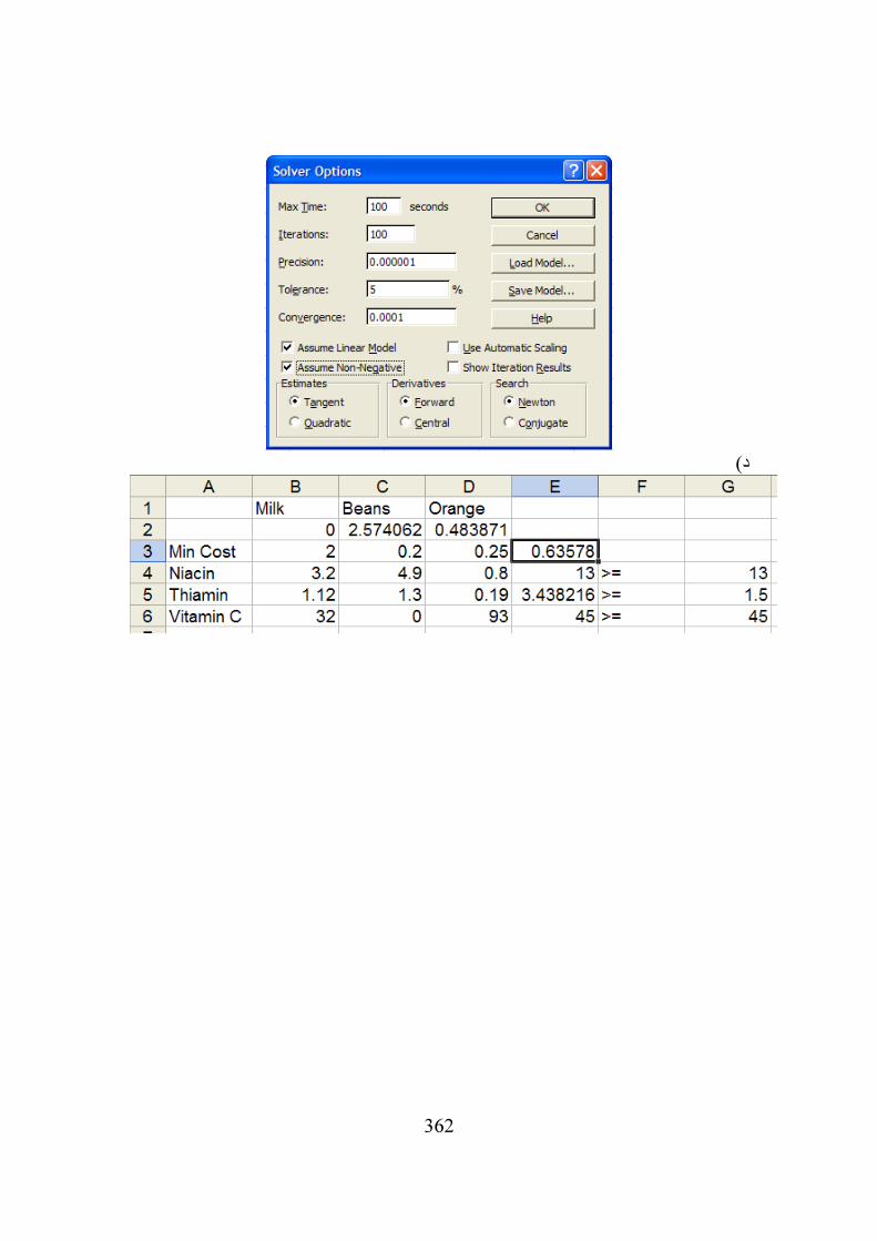
362
د)
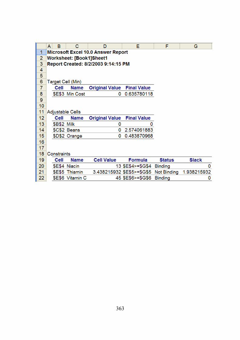
363
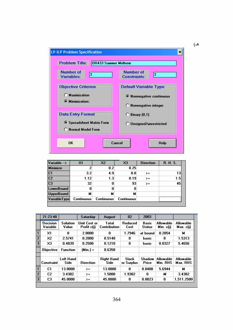
364
هـ)
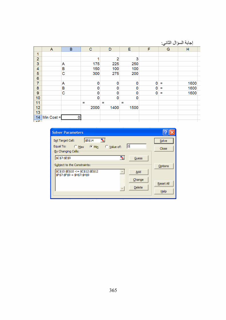
365
إجابة السؤال الثاني:
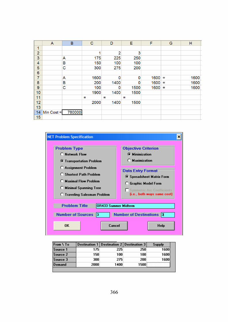
366

367
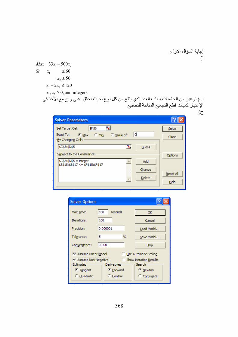
368
إجابة السؤال األول:
ا)1 2
1
2
1 2
1 2
33 500
60
50
2 120
, 0, and integers
Max x x
St x
x
x x
x x
+
≤
≤
+ ≤
≥
ب) نوعين من الحاسبات يطلب العدد الذي ينتج من كل نوع بحيث نحقق أعلى ربح مع األخذ في اإلعتبار كميات قطع التجميع المتاحة للتصنيع.
)ج
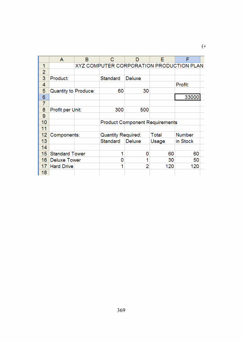
369
د)
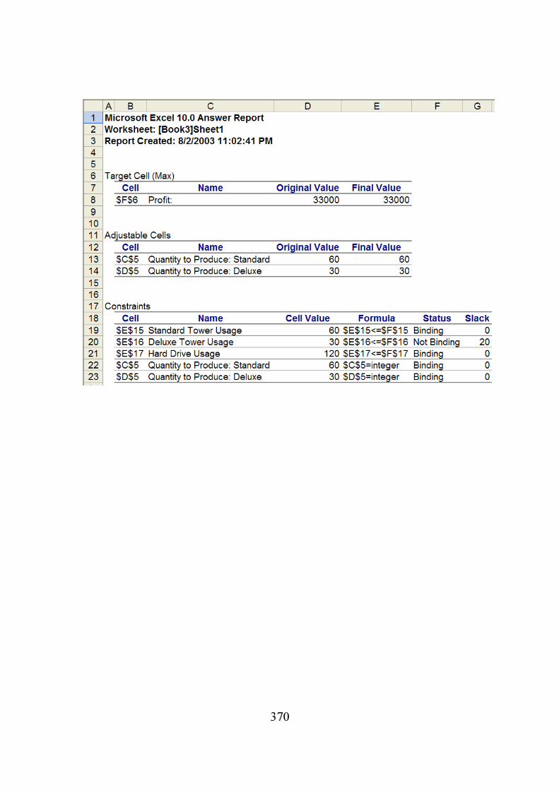
370
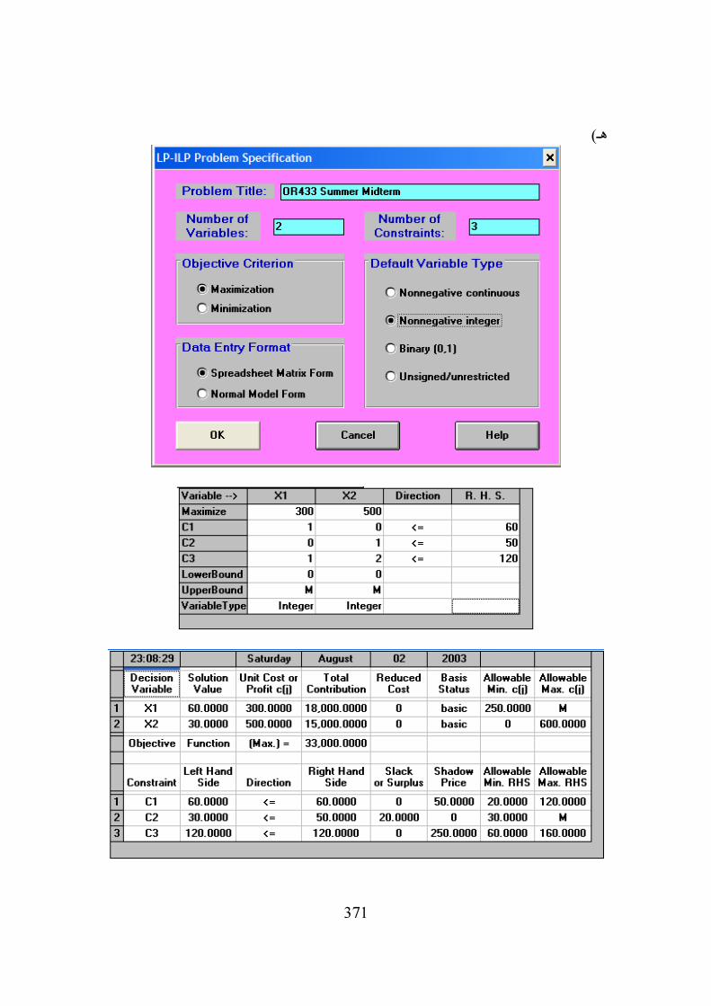
371
هـ)
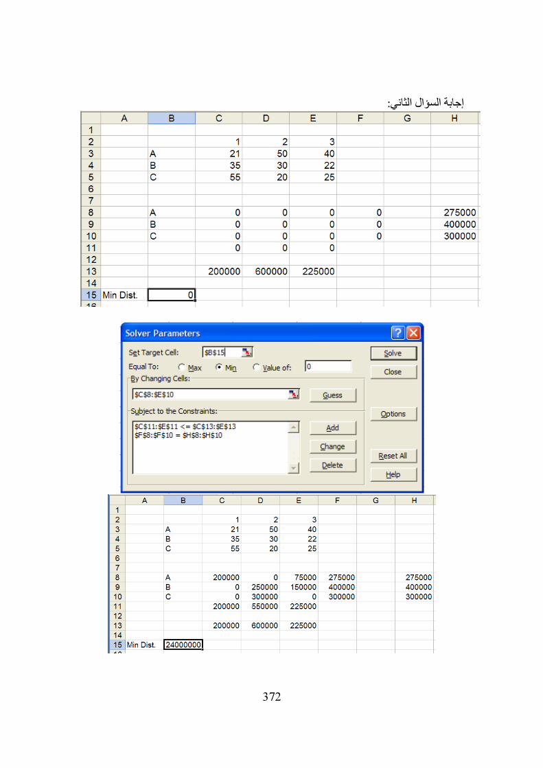
372
إجابة السؤال الثاني:
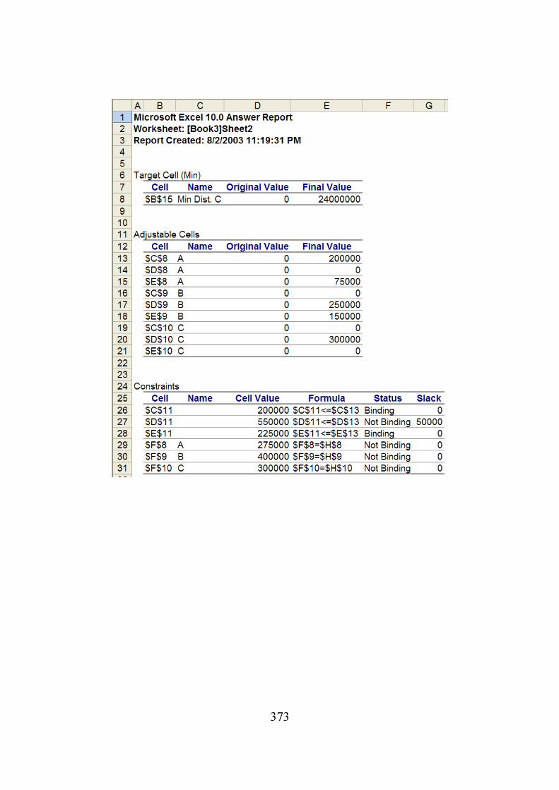
373
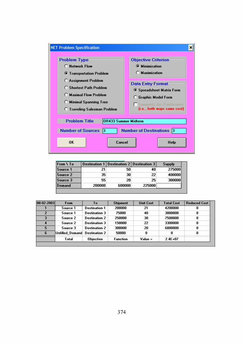
374

375
المراجع:
1- Lawrence, John A., Jr, and Pasternack, Barry A. (2002) Applied
Management Science: Modeling, Spreadsheet Analysis, and Communication for Decision Making. Second Edition. Wiley. 2- Lawrence, John A., Jr, and Pasternack, Barry A. (1998) Applied
Management Science: A Computer-Integrated Approach for Decision Making. Wiley. 3- Microsoft EXCEL Online Help. 4- WINQSB Online Help and Manual. 5- LINDO Online Help. 6- LINGO Online Help. 7- The R Manuals at http://cran.r-project.org/