Statistical InferenceHypothesis Testing

Statistical InferenceHypothesis Testing

Previously, we introduced the point and interval ti ti f k t ( ) d 2estimation of an unknown parameter(s), say µ and σ2.

However, in practice, the problem confronting the scientist or engineer may not be so much the parameter estimation b t rather the formation of aparameter estimation, but rather the formation of a data-based decision procedure that can produce a conclusion about some scientific systemconclusion about some scientific system.

For instanceFor instance,

• an engineer may decide on the basis of sample data whether thean engineer may decide on the basis of sample data whether the true average lifetime of a certain kind of tire is at least 22,000 miles;

• an agronomist may want to decide on the basis of experiments whether one kind of fertilizer produces a higher yield of soybeans th ththan another.

• a manufacturer of pharmaceutical products may decide on the basis of samples whether 90% of all patients given a new medication will recover from a certain disease.

In each of these cases, the scientist or engineer conjectures something about a system.

In addition, each must involve the use of experimental data and decision making that is based on the data.

Formally, in each case, the conjecture can be put in the form of a statistical test of hypothesisthe form of a statistical test of hypothesis.

For instanceFor instance,

• an engineer may decide on the basis of sample data whether the• an engineer may decide on the basis of sample data whether the true average lifetime of a certain kind of tire is at least 22,000 miles;

In the first of above cases, we might say that the engineer has to test th h th i th t θ E(X) 1/λ i t l t 22 000 h th λ ithe hypothesis that θ = E(X) = 1/λ is at least 22,000, where the λ is the parameter of an exponential population;

For instanceFor instance,

• an agronomist may want to decide on the basis of experiments• an agronomist may want to decide on the basis of experiments whether one kind of fertilizer produces a higher yield of soybeans than another.

in the second case we might say that the agronomist has to decide h th > h d th f t lwhether µ1 > µ2, where µ1 and µ2 are the means of two normal

populations;

For instanceFor instance,

• a manufacturer of pharmaceutical products may decide on the basis• a manufacturer of pharmaceutical products may decide on the basis of samples whether 90% of all patients given a new medication will recover from a certain disease.

and in the last case we might say that the manufacturer has to decide h th θ th t f bi i l l ti l 0 90whether θ, the parameter of a binomial population, equals 0.90.

Statistical hypothesisypLet us define precisely what we mean by a statistical hypothesis.

Definition:A statistical hypothesis is an assertion or conjecture or statement about the population usually formulated in terms of populationabout the population, usually formulated in terms of population parameters.

The two complementary statements concerning the population are called null hypothesis H0 and lt ti h th i Halternative hypothesis H1.

Remark that in hypothesis testing, what we are interested most is to test the null hypothesis H0most is to test the null hypothesis H0.

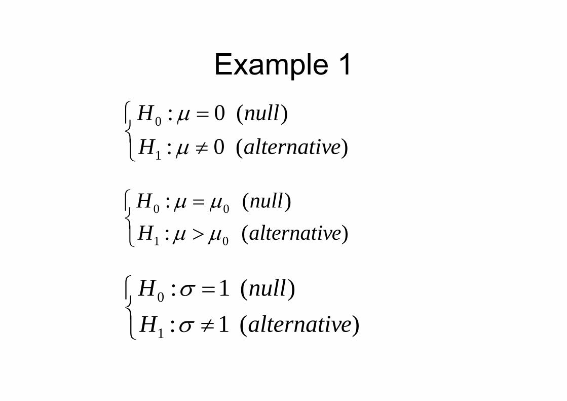
Example 1Example 1⎧ )(0 llH

⎩⎨⎧

≠=

)(0:)(0:

1

0

ealternativHnullH

μμ

⎩ )(1 μ

⎧ = )(: nullH μμ

⎩⎨⎧

>=

)(:)(:

01

00

ealternativHnullH

μμμμ

⎩

⎧ = )(1: nullH σ

⎩⎨⎧

≠=

)(1:)(1:

1

0

ealternativHnullH

σσ

⎩ 1

Example 2Example 2

A test of hypothesisA test of hypothesisDefinition:

A test of statistical hypothesis H is a procedure basedA test of statistical hypothesis H0 is a procedure, based upon the observed values of the random sample obtained, that leads to the rejection or non-rejection of , j jthe hypothesis H0.

For instance, for testing H0: µ = 1, the procedure

2X 0XReject H0 if or2>X 0<Xis a test.

CautionCautionIn statistical hypothesis, we tests H0 against H1, i.e. we observe the datato see if there is enough evidence to reject H0to see if there is enough evidence to reject H0.

• If we have enough evidence to reject H0, we can have great confidence that H0 is false and H1 is true.

• However if we observe the data and find that H0 isHowever, if we observe the data and find that H0 is not rejected, it does not mean that we have great confidence in the truth of H0 . Here it only means that we do not have enough evidence to reject H0.

So in statistical hypothesis we should say "do notSo, in statistical hypothesis we should say "do not reject H0", instead of "accept H0".

In statistical hypothesis, when we draw the conclusion,

Reject H0

i.e. we have enough evidence to reject H0

ORDo not reject H0

i.e. we do not have enough evidence to reject H0

And we never say that

Accept H0

i.e. we have enough evidence to accept H0

Test errorsTest errorsEach test procedure can lead to two kinds of errors.

Type I error: the error of rejecting H0 when it is in fact true.

Each test procedure can lead to two kinds of errors.

yp j g 0

Type II error: the error of not rejecting H0 when it is in fact f lfalse.

N t j t H R j t HNot reject H0 Reject H0

If H0 is true No error Type I errorIf H0 is true No error Type I error

If H0 is false Type II error No error

Error probabilityError probabilityDefineDefine

)|()( 00 trueisHHrejectPerrorITypeP ==α

)|()( 00 falseisHHrejectNotPerrorIITypeP ==β

Ideally we want a test such that these two error probabilitiesIdeally, we want a test such that these two error probabilities can be minimized. However, normally, we cannot control them simultaneously. y

More precisely, there is a trade-off between the two types of M ki ll ill l d t l β d ierror. Making α smaller will lead to a larger β, and vice versa.

(see a picture later)

Therefore in designing a test we can only control one of them say guarantee α in a desired low level and thenthem, say, guarantee α in a desired low level and then try to reduce β as much as we could (i.e. type I error is considered as more serious than type II error).considered as more serious than type II error).

Example 3Example 3S k h h li h b lb d d f d dSuppose we knew that the light bulbs produced from a standard manufacturing process have life times distributed as normal with a standard deviation σ = 300 hours. However, we did not know the mean lifetime µ. For simplicity, assume that we were sure that the mean lifetime should be either 1200 or 1240. Then we may set up the following hypotheses:g yp

⎨⎧ = )(1200:0 nullH μ

⎩⎨ = )(1240:1 ealternativH μ

S th t d l f 100 li ht b lb d th iSuppose that we draw a sample of 100 light bulbs and measure their lifetimes. The sample mean can be used to estimate the true population mean µ.

X

Example 3Example 3Intuitively, a large value of the sample mean will lead to the rejection of the null hypothesis H0. So, if we construct a test asa test as

Reject H0 if ,1249>XThen

)1200|1249()|( XPiHHjP ),1200|1249()|( 00 =>== μα XPtrueisHHrejectP

and

.)1240|1249()|( 00 =≤== μβ XPfalseisHHrejectnotP

a d

Why cannot control the Type I and II errors simultaneously

Rejection/ acceptance regionRejection/ acceptance regionIn Example 3, our test procedure isa p e 3, ou test p ocedu e s

Reject H0 if .1249>XIt means that if the observed value of the random sample,

{ } i l t f th tsay {x1, …, xn}, is an element of the set

{ }1249: >xxx{ } ,1249:,,1 >xxx nK

Then we reject H ; otherwise if the observed valueThen we reject H0; otherwise, if the observed value does not belong to this set, then we do not reject H0.

Rejection/ acceptance regionRejection/ acceptance region

It is easy to see that we partition the sample space of the random sample by to take an action of Xp yrejecting or not rejecting H0.

X

More formally, the partitions of the sample space of the random sample are defined as follows:

Rejection/ acceptance regionRejection/ acceptance regionThe rejection region (or called critical region) of the nullThe rejection region (or called critical region) of the null hypothesis H0 or of the test, denoted by C1, is the set of points in the sample space which leads to thepoints in the sample space which leads to the rejection of H0; while the set of the points in the sample space which leads to the acceptance of H0 is called the acceptance region, denoted by C0.

Th t ti ti d t d fi th j ti i iThe statistic used to define the rejection region is called a test statistic.

Rejection/ acceptance regionRejection/ acceptance regionThe rejection region (or called critical region) of the nullThe rejection region (or called critical region) of the null hypothesis H0 or of the test, denoted by C1, is the set of points in the sample space which leads to thepoints in the sample space which leads to the rejection of H0; while the set of the points in the sample space which leads to the non-rejection of H0 is called the acceptance region, denoted by C0.

Th t ti ti d t d fi th j ti i iThe statistic used to define the rejection region is called a test statistic.

Rejection/ acceptance regionRejection/ acceptance regionThe rejection region (or called critical region) of the nullThe rejection region (or called critical region) of the null hypothesis H0 or of the test, denoted by C1, is the set of points in the sample space which leads to thepoints in the sample space which leads to the rejection of H0; while the set of the points in the sample space which leads to the acceptance of H0 is called the acceptance region, denoted by C0.

Th t ti ti d t d fi th j ti i iThe statistic used to define the rejection region is called a test statistic.

Normally, we use the point estimator of the unknown parameter to be tested in the hypothesis to be our test statistic. For instance, when we want to test the hypothesis of µ, we use the sample mean.

Rejection/ acceptance regionRejection/ acceptance regionIn Example 3, our test procedure isa p e 3, ou test p ocedu e s

Reject H0 if .1249>XThen the rejection region is

Recall that when we design a test of hypothesis, we cannot control the two error probabilities at the same time, and

what we can do is to control the Type I error probability α in a desired low level, (often choose 0.01, 0.05 or 0.1), and then reduce the Type II error probability β as much as we could.

H t d i t t d ith thi t i ti ?How to design a test procedure with this restriction ?

Again, in this example, a large value of the sample mean will l d t th j ti f th ll h th i H S idlead to the rejection of the null hypothesis H0. So, we consider

.

Critical value

How to determine the critical valueHow to determine the critical value

How to determine the critical valueHow to determine the critical value

Thus, the rejection region is

C1 = and we would say that

Suppose that if the observed value of the sample mean is then weSuppose that if the observed value of the sample mean is , then we could conclude that we DO NOT HAVE ENOUGH EVIDENCE TO REJECT H0 at a level α = 0.05.

Power of a testPower of a test

Power of a testPower of a testβ = 0 6225 so 1 - β = 0 3775 i eβ = 0.6225, so 1 - β = 0.3775, i.e.

P( Reject H0 | H0 is false) = 0.3775

A power of a testA power of a testis a quantity to evaluate the goodness of a test.

For the comparison of two tests, first we need both tests to have a common α, and then the test is better if it has a higher powerhigher power.

Power of a testPower of a testIncrease the power of a test 1- βIncrease the power of a test, 1- β

Decrease the Type II error probability β

Increase the Type I error probability α

So, how to increase the power of a test and the value αremains unchanged?

400,

Therefore, the rejection region becomes . j g

Now, let’s calculate the power of this test with n = 400 and α = 0.05.

Power = 0.3775

(n=100 α = 0 05)

Power = 0.8466

(n=400 α = 0 05)(n=100, α = 0.05) (n=400, α = 0.05)

QuestionQuestion

Similarly, we will also consider these tests for σ2.