Chapter 1 COMPLEX ANALYSIS - 國立臺灣大學cc.ee.ntu.edu.tw/~jfkiang/complex analysis/complex_analysis.pdfChapter 1 COMPLEX ANALYSIS Jean-Fu Kiang Department of Electrical Engineering

Chapter 1

COMPLEX ANALYSIS

Jean-Fu KiangDepartment of Electrical Engineering andGraduate Institute of Communication EngineeringNational Taiwan UniversityTaipei, Taiwan, ROC

Abstract In this Chapter, fundamental concepts and theories of complex functionsare reviewed, and skills of complex analysis are practiced.

Keywords: Riemann sheet, branch, branch point, branch cut, singularity, pole, zero,limit, continuity, analyticity, Cauchy-Riemann equations, harmonic func-tion, elementary function, analytic continuation, contour integral, MLtheorem, Green’s theorem, Cauchy’s theorem, Cauchy’s integral for-mula, Taylor series, geometric series, convergence test, Taylor’s theorem,Laurent theorem, residue theorem, improper integral, principal value,Kramers-Kronig relation, Landau damping, inverse Laplace transform,conformal mapping, boundary-value problem, potential, streamline, bi-linear transformation, Schwarz-Christoffel transformation, Poisson inte-gral formula.

1. Basic OperationsA complex number z is represented as z = x+ iy with real part x and

imaginary part y. Both x and y are real numbers and are independentof each other, i =

√−1 is an imaginary unit to mark the imaginary part.

The complex conjugate of z is defined as z∗ = x−iy, which has the samereal part as z, and imaginary part of opposite sign to z. Hence, the realand imaginary parts of z can be retrieved as x = Re(z) = (z +z∗)/2 andy = Im(z) = (z − z∗)/(2i), respectively.

Let z1 = x1 + iy1 and z2 = x2 + iy2. Two complex numbers are equalif and only if both their real and imaginary parts are equal. In otherwords, z1 = z2 if and only if x1 = x2 and y1 = y2. The operation ofaddition(subtraction) is performed by adding(subtracting) the real part

2 Fundamentals of Electrical Engineering

and imaginary part, respectively, of the two operands, namely, z1±z2 =(x1 ± x2) + i(y1 ± y2).

Since a complex number is consisted of two independent parts, themultiplication of two complex numbers renders four items as z1z2 =x1x2 + x1iy2 + iy1x2 + iy1iy2 = (x1x2 − y1y2) + i(x1y2 + y1x2). Thedivision of z1 by z2 is facilitated by multiplying both the numerator andthe denominator with z∗2 to make a real denominator, namely,

z1

z2=

z1z∗2

z2z∗2

=(x1x2 + y1y2) + i(y1x2 − x1y2)

(x22 + y2

2)

The operations of addition and multiplication follow the commuta-tive rule that the operation outcome is independent of the order ofthe operands, namely, z1 + z2 = z2 + z1 and z1z2 = z2z1. They alsosatisfy the associative rule that when three operands are operated intwo steps, the outcome is independent of the order of steps, namely,z1 + (z2 + z3) = (z1 + z2) + z3 and z1(z2z3) = (z1z2)z3. The distributiverule is defined between the two operations as z1(z2 + z3) = z1z2 + z1z3.

Figure 1.1. A complex number viewed as coordinates or position vector.

Geometrical Interpretation. The real and the imaginary parts canbe marked as the x and y coordinates, respectively, of a point P on thetwo-dimensional Cartesian plane as shown in Fig.1.1. A two-dimensionalvector V can be defined by setting the origin as the starting point, andpoint P as the ending point. Then, the complex number z = x + iy, thecoordinates (x, y), and the vector V = OP = xx+yy, are commensurate.In other words, the basic operations and rules defined for the complexnumbers are also observed by the Cartesian coordinates and the two-dimensional vectors.

Some properties of complex numbers can be appreciated from thegeometrical point of view. For example, the modulus or absolute value

Complex Analysis 3

of z, |z|, is equivalent to the length of the vector,∣∣∣OP

∣∣∣, or the distancefrom O to P .

The triangle inequalities |z1+z2| ≤ |z1|+ |z2| and |z1 +z2| ≥ |z1|−|z2|can be interpreted geometrically as: the sum of the lengths of any twosides of a triangle is larger than that of the third side, the difference ofthe lengths of any two sides of a triangle is less than that of the thirdside.

A complex number can be expressed in the polar form as z = r(cos θ+i sinθ) = r 6 θ, where r = |z| =

√x2 + y2 is the magnitude or modulus of

z, and θ = arg(z) = tan−1 (y/x) is the argument of z. Note that thereare an infinite number of arguments for the same z, which are related toa uniquely defined principal argument Arg(z) by arg(z) = Arg(z)+2nπ,where n is any integer and −π < Arg(z) ≤ π.

The multiplication of z1 and z2 can thus be succinctly expressed asz1z2 = r1r2[cos(θ1 + θ2) + i sin(θ1 + θ2)], and the division of z1 by z2 asz1/z2 = (r1/r2)[cos(θ1 − θ2) + i sin(θ1 − θ2)] if z2 6= 0. By induction, wehave zn = rn(cosnθ + sinnθ). By setting |z| = r = 1, the de Moivre’sformula, (cos θ + i sinθ)n = cosnθ + i sinnθ, is recovered.

Define the nth root of z as w = z1/n if z 6= 0, or equivalently, wn =z. Let w = ρ(cosφ + i sinφ) and z = r(cos θ + i sinθ), the definitionimplies that ρn(cosnφ + i sinnφ) = r(cos θ + i sinθ), or ρ = r1/n, φ =(θ + 2kπ)/n with k = 0, 1, 2, · · · , n − 1. These n distinctive roots canbe expressed as wk = r1/n [cos(θ/n + 2kπ/n) + i sin(θ/n + 2kπ/n)] withk = 0, 1, 2, · · · , n − 1, among which w0 is called the principal root of z.

2. Analytic Functions

Figure 1.2. Neighborhood of z0.

Point Set. As shown in Fig.1.2, the ρ-neighborhood of z0 = x0 + iy0

is defined as an open disk of radius ρ, centerd at z0. It is symbolizedas Nρ(z0) = {z| |z − z0| < ρ}. A point z0 is an interior point of a setS if and only if there exists a neighborhood Nδ(z0) that belongs in S.


A set S is open if and only if every z in S is an interior point. The setS = {z| ρ1 < |z − z0| < ρ2} is called an open annulus.

A point zb is called the boundary point of S if every Nδ(zb) containsat least one point in S and at least one point not in S. The boundaryof S contains all the boundary points of S.

An open set S is called connected if any pair of points, z1 and z2, inS can be connected by a polygonal contour that lies entirely in S. A setS is called a domain if and only if S is an open connected set.

A function w = f(z) is a rule of mapping a complex number in a set Don the z-plane into another complex number in a set R in the w-plane.The set D is called the domain of f , and the set R = {w| w = f(z), z ∈D} is called the range of f .

Figure 1.3. Neighborhoods used to demonstrate limit.

Limit. Assume function f(z) is defined in Nδ(z0), except possiblyat z0 itself. This function is said to have a limit at z0, lim

z→z0f(z) = L,

if and only if that for any infinitesimal ε > 0, there exists another in-finitesimal δ > 0 such that |f(z)−L| < ε whenever 0 < |z − z0| < δ. Asdemonstrated in Fig.1.3, for all Nε(L) = {w| |w − L| < ε}, there existsan Nδ(z0) = {z| 0 < |z − z0| < δ} such that w = f(z) falls in Nε(L)whenever z falls in Nδ(z0).

If limz→z0

f(z) = L1 and limz→z0

g(z) = L2, then limz→z0

[f(z) + g(z)] = L1 + L2,

limz→z0

f(z)g(z) = L1L2, and limz→z0

f(z)/g(z) = L1/L2 if L2 6= 0.

Continuity. Function f(z) is continuous at z0 if limz→z0

f(z) = f(z0),

namely, the limit of the function at z0 is the same as the value of f(z)at z0. Note that as taking the limit of a function, the argument z neverreaches z0 although it can be as close as desired to z0.

Complex Analysis 5

If two functions f(z) and g(z) are continuous at z0, then f(z) + g(z)and f(z)g(z) are continuous at z0, and f(z)/g(z) is continuous at z0 ifg(z0) 6= 0.

Derivative. The differential of a complex number z is defined as∆z = ∆x + i∆y. Assume function f(z) is defined in Nδ(z0). Thederivative of f(z) exists at z0 and is expressed as f ′(z0) if and only iff ′(z0) = lim

∆z→0[f(z0 + ∆z) − f(z0)]/∆z is the same with arbitrary choices

of ∆x and ∆y. The function f(z) is differentiable at z0 if f ′(z0) exists.If f(z) and g(z) are differentiable at z and c is a constant, then the

same rules of differentiation as in real variables apply, namely,

dc/dz = 0, [cf(z)]′ = cf ′(z), [f(z) + g(z)]′ = f ′(z) + g′(z)[f(z)g(z)]′ = f ′(z)g(z) + f(z)g′(z)[f(z)/g(z)]′ = [g(z)f ′(z)− f(z)g′(z)]/g2(z)(d/dz)f [g(z)] = f ′[g(z)]g′(z)

Analyticity. Function f(z) is analytic at z0 if and only if f(z) isdifferentiable at z0 and at every point of Nδ(z0). The function f(z) isanalytic in a domain D if and only if f(z) is analytic at every point inD.

Note that analyticity at a point is a property prevailing over its neigh-borhood, while differentiability is a property which is required only atthat point. For example, f(z) = |z|2 is differentiable at z = 0, butnowhere else is differentiable. By definition, it is nowhere analytic. Takeanother example, f(z) = z2 is differentiable everywhere in the z-plane,hence is also analytic everywhere. Function f(z) is called an entire func-tion if and only if it is analytic over the whole z-plane.

3. Cauchy-Riemann EquationsFunction f(z) can be explicitly decomposed into real and imaginary

parts as f(z) = u(x, y) + iv(x, y), where both u(x, y) and v(x, y) arereal functions of x and y. If f(z) is differentiable at z, the derivative off(z) defined as f ′(z) = lim

∆z→0[f(z + ∆z) − f(z)]/∆z exists for arbitrary

∆z. Firstly, let ∆y = 0, then ∆z = ∆x, and f ′1(z) = ∂u(x, y)/∂x +

i∂v(x, y)/∂x. Next, let ∆x = 0, then ∆z = i∆y, and f ′2(z) = −i∂u(x, y)/∂y+

∂v(x, y)/∂y. Since f ′1(z) = f ′

2(z) by definition, we have

∂u

∂x=

∂v

∂y,

∂u

∂y= −∂v

∂x(1.1)

These are called the Cauchy-Riemann equations, which are the necessaryconditions of the analyticity of f(z) at z.


Next, to prove that (1.1) are also the sufficient conditions of the an-alyticity of f(z) at z, assume that the Cauchy-Riemann equations holdat all points in D, for example, at z0 = (x0, y0), then

f(z0 + ∆z) − f(z0) = [u(x0 + ∆x, y0 + ∆y)− u(x0, y0)]+i [v(x0 + ∆x, y0 + ∆y) − v(x0, y0)]

'[ux(x0, y0)∆x + uy(x0, y0)∆y + uxx(x0, y0)(∆x)2

+2uxy(x0, y0)∆x∆y + uyy(x0, y0)(∆y)2]

+i[vx(x0, y0)∆x + vy(x0, y0)∆y + vxx(x0, y0)(∆x)2

+2vxy(x0, y0)∆x∆y + vyy(x0, y0)(∆y)2]

' [ux(x0, y0) + ivx(x0, y0)] (∆x + i∆y) (1.2)

where µα is the first derivative of µ with respect to α with µ = u, v,α = x, y, and µαβ is the second derivative. The second approximationis obtained by imposing the Cauchy-Riemann equations and neglectingthe second-order terms when ∆x and ∆y are sufficiently small. Eq.(1.2)implies that f ′(z0) = lim

∆z→0[f(z0 + ∆z) − f(z0)]/∆z exists at every point

in D. Thus, f(z) is analytic in D. The Cauchy-Riemann equations areoften used to check the analyticity of a complex function.

Harmonic Functions. Function φ(x, y) is called a harmonic func-tion in D if the derivatives of φ(x, y) up to the second order is continuousand φ(x, y) satisfies the Laplace equation

(∂2

∂x2+

∂2

∂y2

)φ(x, y) = 0

An analytic function f(z) = u(x, y) + iv(x, y) satisfies the Cauchy-Riemann equations. Thus, we have

∂2u

∂x2=

∂

∂x

(∂u

∂x

)=

∂

∂x

(∂v

∂y

)=

∂

∂y

(∂v

∂x

)=

∂

∂y

(−∂u

∂y

)= −∂2u

∂y2

By definition, u(x, y) is a harmonic function, and v(x, y) can be provento be a harmonic function in a similar way. Since u(x, y) and v(x, y) con-stitute an analytic function in D, they are called the conjugate harmonicfunction of each other.

4. Elementary FunctionsExponential Function. The complex exponential function is de-

fined in the same way as its real counterpart. By definition, ez = ex+iy =

Complex Analysis 7

exeiy = ex(cos y + i siny). Since ez is analytic for all z, it is an entirefunction.

When y = 0, ez is reduced to the real exponential function ex. Suchan extension of domain from the real axis to the whole complex planeis called analytic continuation, which is commonly practiced as long asthe definition is consistent with the original one when z is reduced to x.

Function ez is periodic with a complex period of 2πi, namely, ez+2nπi =eze2nπi = ez for all z. Thus, the z-plane can be divided into hori-zontal strips Sn = {z = x + iy| (2n − 1)π < y ≤ (2n + 1)π} withn = 0,±1,±2, · · ·. Each Sn is called a branch of ez , and the functionalvalues over Sn are replica of those in the other branches. The stripS0 = {z = x + iy| − π < y ≤ π} is called the principal branch of ez .

Logarithmic Function. The logarithmic function w = ln z can bedefined in terms of the exponential function as ew = z. Let w = u + iv,then z = reiθ = ew = eu+iv = eueiv. By comparison, we have u = ln r =loge |z|, v = θ = θ0 + 2nπ, where θ = arg(z), −π < θ0 = Arg(z) ≤π, n = 0,±1,±2, · · ·. In short, ln z = ln |z| + i[Arg(z) + 2nπ] withn = 0,±1,±2, · · ·. The principal branch of ln z is defined as Ln z =ln |z| + iArg(z).

If a point is rotated counterclockwise in the z-plane along a circlecentered at the origin, it will return to where it starts. The value ofz remains the same, but the argument of z is incremented by 2π, andln z is incremented by i2π. It can be understood as if the point sweepsacross a branch cut and moves into another branch or another Riemannsheet. The definition of the principal branch with −π < Arg(z) ≤ πimplies that the branch cut is chosen at Arg(z) = π. The branch cutcan be arbitrarily chosen for convenience. However, its position shouldbe fixed throughout the whole derivation to maintain consistency. Theend points of a branch cut is called the branch points.

Note that Ln z is not continuous across the branch cut, Arg(z) ap-proaches π when z approaches the branch cut from the upper half-plane,and Arg(z) approaches −π when z approaches the branch cut from thelower half-plane, hence a discontinuity exists across the branch cut.Other than the branch cut, Ln z is analytic in D = {z| z 6= 0,−π <Arg(z) < π}.

The complex power zα with z 6= 0 and α complex can be manipulatedas zα = eα ln z which has an infinite number of branches. The principalbranch can similarly be denoted as eαLn z.

Trigonometric and Hyperbolic Functions. The complex trigono-metric functions can be extended from one of the definitions of real


trigonometric functions as

sin z =eiz − e−iz

2i, cos z =

eiz + e−iz

2, tan z =

sin z

cos z

cot z =1

tan z, sec z =

1cos z

, csc z =1

sin z

Likewise, the complex hyperbolic functions can be extended from theirreal counterparts as

sinh z =ez − e−z

2, cosh z =

ez + e−z

2, tanh z =

sinh z

cosh z

coth z =1

tanh z, sech z =

1cosh z

, csch z =1

sinh z

The same differential rules for the real functions apply as

d

dzsin z = cos z,

d

dzcos z = − sin z

d

dztan z = sec2 z,

d

dzcot z = − csc2 z

d

dzsec z = sec z tan z,

d

dzcsc z = − csc z cot z

d

dzsinh z = cosh z,

d

dzcosh z = sinh z

The inverse trigonometric functions can be defined in terms of thecomplex trigonometric functions. For example, the inverse sinusoidalfunction w = sin−1 z is equivalent to z = sinw. Thus, we have z =sinw = (eiw − e−iw)/(2i), or e2iw − 2izeiw − 1 = 0. The solutions areeiw = iz ±

√1 − z2 = iz + (1 − z2)1/2. Note that

√α is the principal

value of α1/2.By differentiating both sides of z = sinw with respect to z, we have

1 = (d sinw/dw)(dw/dz) = cos w(dw/dz), or dw/dz = 1/ cosw = (1 −z2)−1/2.

5. Contour IntegralsThe parametric representation of a curve in the z-plane is C = {z| z(t) =

x(t) + iy(t), a ≤ t ≤ b} with t as the parameter. Curve C is a smoothcurve if x′(t) and y′(t) are continuous on a ≤ t ≤ b. Curve C is piece-wise smooth if C can be decomposed into pieces of smooth curves Cj as

C =n∑

j=1

Cj . Curve C is called a simple curve if C does not cross itself.

Curve C is a closed curve if its starting point and ending point are thesame.

Complex Analysis 9

Figure 1.4. Partition of a contour in the z-plane.

A contour is defined as a piecewise smooth curve. Given a contourC = {z | z(t) = x(t) + iy(t), a ≤ t ≤ b}, and f(z) = u(x, y) + iv(x, y) isa complex function defined at all points on C. Fig.1.4 shows that the

contour C is partitioned into many infinitesimal curves as C =n∑

j=1

Cj

with a = t0 < t1 < · · · < tn = b. Let the value of z at tk be zk = z(tk)with k = 0, 1, 2, · · · , n, and ∆zk = zk − zk−1 with k = 1, 2, · · · , n.

The mean-value theorem states that a zk on Ck can be found suchthat

∫

Ck

f(z)dz = f(zk)∆zk where zk = z(tk) with tk−1 ≤ tk ≤ tk . Define

the norm of a partition as ||P || = |∆zk|max. The integral of a complexfunction f(z) along the contour C can thus be calculated as

∫

C

f(z)dz = lim||P ||→0

n∑

k=1

f(zk)∆zk (1.3)

Expressing f(z) as u(x, y)+ iv(x, y), then the contour integral in (1.3)can be calculated as

∫

C

f(z)dz = lim||P ||→0

n∑

k=1

(uk + ivk)(∆xk + i∆yk)

= lim||P ||→0

n∑

k=1

[(uk∆xk − vk∆yk) + i(vk∆xk + uk∆yk)]

=∫

C

(udx− vdy) + i

∫

C

(vdx + udy) (1.4)

which is the sum of two contour integrals of real functions. Furthermore,if both x and y are expressed in terms of the parameter t, namely,


dx = x′(t)dt and dy = y′(t)dt, then (1.4) can be reduced to∫

C

f(z)dz =∫

C

f [z(t)]z′(t)dt

=∫

C

[u(x(t), y(t))x′(t) − v(x(t), y(t))y′(t)

]dt

+i

∫

C

[v(x(t), y(t))x′(t) + u(x(t), y(t))y′(t)

]dt

The differential path length can be expressed as ds =√

(dx)2 + (dy)2 =√[x′(t)]2 + [y′(t)]2dt = |z′(t)|dt = |dz|, The total length of C can thus

be expressed as L =∫ b

a|z′(t)|dt.

ML Inequality. If C is a smooth curve with total length L, f(z) iscontinuous on C and has a maximum value of M on C, we have

∣∣∣∣∣n∑

k=1

f(zk)∆zk

∣∣∣∣∣ ≤n∑

k=1

|f(zk)| |∆zk| ≤ Mn∑

k=1

|∆zk |

≤ Mn∑

k=1

Lk = ML

In other words,

∣∣∣∣∣∣

∫

C

f(z)dz

∣∣∣∣∣∣=

∣∣∣∣∣ lim||P ||→0

n∑

k=1

f(zk)∆zk

∣∣∣∣∣ ≤ ML, which is re-

ferred to as the ML inequality.Green’s Theorem. Let domain D be simply connected, C is a

simple closed contour in D, R is the region enclosed by C, u(x, y) andv(x, y) are functions whose first derivatives are continuous in D. TheGreen’s theorem relates the contour integral of u(x, y) and v(x, y) withthe surface integral of their derivatives as

∮

C

[u(x, y)dx + v(x, y)dy] =∫∫

R

(∂v

∂x− ∂u

∂y

)dxdy (1.5)

By analog, consider a two-dimensional electric field distribution E(x, y) =xu(x, y) + yv(x, y). The Stokes’ theorem states that

∮

C

E · ds =∫∫

R

∇× E · da

where C is a closed contour on the xy-plane encircling a region R. Theexpansion gives the same results as (1.5).

Complex Analysis 11

6. Cauchy’s TheoremThe Cauchy’s theorem states that if f(z) is analytic in a simply

connected domain D, and C is any simple closed contour in D, then∮

C

f(z)dz = 0.

The proof is straightforward. Since f(z) = u(x, y) + iv(x, y) is an-alytic, the Cauchy-Riemann equations imply that ∂u/∂x = ∂v/∂y and∂u/∂y = −∂v/∂x. The contour integral thus is reduced to

∮

C

f(z)dz =∮

C

(u + iv)(dx + idy) =∮

C

(udx− vdy) + i

∮

C

(vdx + udy)

=∫∫

R

(−∂v

∂x− ∂u

∂y

)dxdy + i

∫∫

R

(∂u

∂x− ∂v

∂y

)dxdy = 0

where the Green’s theorem is applied to transform the contour integralsinto surface integrals.

Figure 1.5. Close contours in domain D with two holes.

Contour Deformation. If f(z) is analytic in a domain D which hasa hole as shown in Fig.1.5. Assume C and C1 are simple closed contourssuch that C1 encloses the hole and is interior to C. A new contour Kcan be defined by connecting C and C1 with two line segments AB andBA. Hence, f(z) is analytic on and within contour K, which impliesthat

∮

K

f(z)dz =

∮

C

+∫

AB

+∮

−C1

+∫

BA

f(z)dz = 0


Since the integrals along AB and BA, respectively, cancel each other,we have ∮

C

f(z)dz = −∮

−C1

f(z)dz =∮

C1

f(z)dz

This implies that the contour of integration can be deformed arbitrarilyas long as it stays in the domain D.

In case the domain D contains multiple holes as shown in Fig.1.5, thecontour C encloses all the holes, while contour Ck encloses the kth hole.Pairs of overlapping line segments are placed to link all the Ck contoursto C to form a closed contour K which encloses no holes, and f(z) isanalytic on and within the contour K. By using the same argument, wehave

∮

C

f(z)dz =n∑

k=1

∮

Ck

f(z)dz

This implies that a closed contour can be deformed arbitrarily into anumber of closed contours, with each one enclosing a hole.

Figure 1.6. Contours with the same starting and ending points.

Fig.1.6 shows two separate contours, C1 and C2, both are drawn fromz0 to z1. A closed contour K can be defined as the concatenation of C1

and −C2. Assume there is no hole within K, thus no hole is encounteredwhen contour C1 is deformed into C2. Then, the Cauchy’s theoremimplies that∮

K

f(z)dz =∫

C1

f(z)dz +∫

−C2

f(z)dz =∫

C1

f(z)dz −∫

C2

f(z)dz = 0

or∫

C1

f(z)dz =∫

C2

f(z)dz. This implies that the contour integral depends

only on the end points, and the contour of integration can be deformedarbitrarily as long as it does not cross any hole.

Complex Analysis 13

Existence of Antiderivative. The rules of contour integration aresimilar to those of one-dimensional integration of real functions. Forexample,

F (z) =∫

f(z)dz is the antiderivative of f(z)

if and only if F ′(z) = f(z) for all z in D∫

C

f(z)dz =∫ z1

z0

f(z)dz = F (z1) − F (z0)

∫

C

f(z)dz =b∫

a

F ′[z(t)]z′(t)dt =∫ b

a

d

dtF [z(t)]dt

= F [z(t)]|t=bt=a = F [z(b)]− F [z(a)] = F (z1) − F (z0)

where z = z0 at t = a and z = z1 at t = b.Assume f(z) is analytic in D, let z0 be a fixed point in D, and z be

any point in D. Define F (z) =∫ z

z0

f(s)ds, then

F (z + ∆z) − F (z) =∫ z+∆z

z0

f(s)ds −∫ z

z0

f(s)ds =∫ z+∆z

zf(s)ds

andF (z + ∆z)− F (z)

∆z− f(z) =

1∆z

∫ z+∆z

z[f(s)− f(z)]ds (1.6)

Since f(z) is analytic at z, it is also continuous at z. Thus, for any ε > 0,there exists a δ > 0 such that |f(s) − f(z)| < ε whenever |s − z| < δ.Choosing ∆z such that |∆z| < δ, (1.6) can be reduced to

∣∣∣∣F (z + ∆z) − F (z)

∆z− f(z)

∣∣∣∣ =∣∣∣∣

1∆z

∣∣∣∣

∣∣∣∣∣

∫ z+∆z

z[f(s) − f(z)]ds

∣∣∣∣∣

<1

|∆z|ε|∆z| = ε

Thus, we have F ′(z) = lim∆z→0

F (z + ∆z) − F (z)∆z

= f(z) for all z in D.

7. Cauchy’s Integral FormulaIf f(z) is analytic in a simply connected domain D, C is a simple closed

contour in D, z0 is any point within C, then f(z0) =1

2πi

∮

C

f(z)z − z0

dz,

which is the Cauchy’s integral formula.


Since f(z) is analytic in D,f(z)

z − z0is analytic in D except at z = z0.

Let C1 = {z | |z − z0| = r} be a circle within C, then the contour ofintegration C can be deformed to C1. Thus, we have

∮

C

f(z)z − z0

dz =∮

C1

f(z)z − z0

dz =∮

C1

f(z0) + f(z)− f(z0)z − z0

dz

= f(z0)∮

C1

dz

z − z0+∮

C1

f(z)− f(z0)z − z0

dz = 2πif(z0)

The last step can be proved as follows. Since f(z) is analytic at z0,it is continuous at z0. For any ε > 0, there exists a δ > 0 such that|f(z) − f(z0)| < ε whenever |z − z0| < δ. The radius of C1 is chosen tobe δ/2, namely, |z−z0| = δ/2. Thus, |[f(z)− f(z0)]/(z − z0)| ≤ ε/(δ/2)

for z on C1, hence∣∣∣∣∮

C1

f(z) − f(z0)z − z0

dz

∣∣∣∣ ≤(

ε

δ/2

)(2π

δ

2

)= 2πε which

can be arbitrarily small. On C1, z = z0 + (δ/2)eiθ, dz = i(δ/2)eiθdθ,

hence∮

C1

dz

z − z0= 2πi.

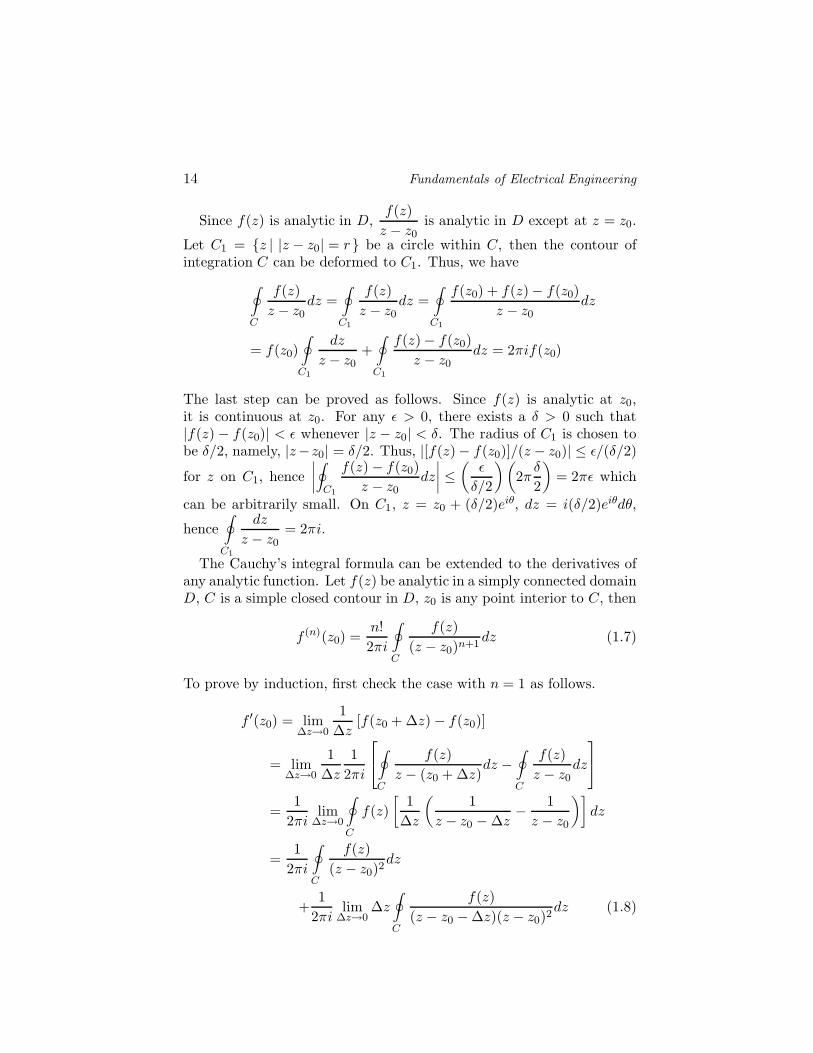
The Cauchy’s integral formula can be extended to the derivatives ofany analytic function. Let f(z) be analytic in a simply connected domainD, C is a simple closed contour in D, z0 is any point interior to C, then

f (n)(z0) =n!2πi

∮

C

f(z)(z − z0)n+1

dz (1.7)

To prove by induction, first check the case with n = 1 as follows.

f ′(z0) = lim∆z→0

1∆z

[f(z0 + ∆z) − f(z0)]

= lim∆z→0

1∆z

12πi

∮

C

f(z)z − (z0 + ∆z)

dz −∮

C

f(z)z − z0

dz

=1

2πilim

∆z→0

∮

C

f(z)[

1∆z

(1

z − z0 − ∆z− 1

z − z0

)]dz

=1

2πi

∮

C

f(z)(z − z0)2

dz

+1

2πilim

∆z→0∆z

∮

C

f(z)(z − z0 − ∆z)(z − z0)2

dz (1.8)

Complex Analysis 15

where the identity [1/(z − z0 − ∆z) − 1/(z − z0)]/∆z = 1/(z − z0)2 +∆z/[(z−z0−∆z)(z−z0)2] has been used. Since f(z) is analytic in D, it iscontinuous and bounded on C, namely, |f(z)| ≤ M for all z on C. Let δbe the shortest distance of |z− z0| among all z’s on C, then |z− z0| ≥ δ,1/|z − z0|2 ≤ 1/δ2, |f(z)|/|z − z0|2 ≤ M/δ2 for all z on C. Choose|∆z| ≤ δ/2, then |z − z0 − ∆z| ≥ ||z − z0| − |∆z|| ≥ δ − |∆z| ≥ δ/2,1/|z − z0 − ∆z| ≤ 2/δ for all z on C, hence

∣∣∣∣∣∣∆z

∮

C

f(z)(z − z0 − ∆z)(z − z0)2

dz

∣∣∣∣∣∣≤ |∆z|

(2δ

)(M

δ2

)L

= 2ML|∆z|δ3

= ε

where L is the length of C, and ε can be arbitrarily small if ∆z ap-proaches zero faster than δ3. Thus, the last term in (1.8) approacheszero, and

f ′(z0) =1!2πi

∮

C

f(z)(z − z0)1+1

dz

The cases with n ≥ 2 can be proved in the same way.If f(z) is analytic at z0, its nth derivative can be obtained from (1.7),

which implies that an analytic function possesses derivatives of any or-der.

Liouville’s Theorem. Let the contour of integration C in (1.7) be acircle with radius R and length L = 2πR, namely, C = {z| |z−z0| = R}.Assume |f(z)| ≤ M for z on C, then

|f (n)(z0)| =

∣∣∣∣∣∣n!2πi

∮

C

f(z)(z − z0)n+1

dz

∣∣∣∣∣∣

=n!2π

∣∣∣∣∣∣

∮

C

f(z)(z − z0)n+1

dz

∣∣∣∣∣∣≤ n!

2π

(M

Rn+1

)(2πR) =

n!MRn

which is named the Cauchy inequality.If f(z) is a bounded entire function with |f(z)| ≤ M for all z, the

Cauchy inequality implies that |f ′(z0)| ≤ M/R. Let R approach infinity,then |f ′(z0)| approaches zero for all z0, which implies that f(z) is aconstant. In other words, the only bounded entire function is a constant.

8. Taylor SeriesComplex Sequence. A complex sequence is a set of complex num-

bers zn’s arranged in order with integer index n, denoted as {zn}. This


sequence converges to a complex number L, expressed as zn → L orlim

n→∞zn = L, if and only if for any given infinitesimal ε > 0, there exists

a positive integer N such that |zn−L| < ε for n > N . The sequence {zn}diverges if it does not converge. The sequence can be decomposed intotwo real sequences {xn} and {yn} where zn = xn + iyn. Let L = a + ib,then zn → L implies that xn → a and yn → b.

Complex Series. The nth partial sum of a given complex sequence

{zn} is defined as Sn =n∑

k=1

zk. If the limit of the nth partial sum as

n → ∞ exists, it is called the series of the sequence {zn}, denoted as

S∞ = limn→∞

Sn =∞∑

k=1

zk. The nth partial sum diverges if it does not

converge.Geometric Series. If the sequence {zn} is consisted of consecutive

powers of a given complex number, namely, zn = zn−1, then its asso-ciated series is called a geometric series. The nth partial sum of thegeometric sequence can be calculated as Sn = (1− zn)/(1− z), and willconverge to 1/(1− z) if |z| < 1.

Note that if the sequence {zn} converges to a nonzero number c, thenth partial sum, with n greater than a threshold N , will be incrementedby c whenever n is incremented by one. Thus, the series will diverge.

A series∞∑

k=1

zk is called absolutely convergent if the series formed of

the absolute value of the original sequence converges, namely,∞∑

k=1

|zk|

converges. It is obvious that the original series converges if it is abso-lutely convergent, but not vice versa.

Convergence Tests. Ratio test and root test are two alternativetechniques to check the convergence of a sequence. In the ratio test, the

limit of two consequent terms in a sequence is calculated as limn→∞

∣∣∣∣zn+1

zn

∣∣∣∣ =L. In the root test, the nth root of the nth term is calculated as

limn→∞

n√|zn| = L. In either test, the series

∞∑

k=1

zk is absolutely conver-

gent if L < 1, is divergent if L > 1, and is inconclusive if L = 1.Power Series. Let z0, a0, a1, · · ·, ak, · · · be given complex numbers.

The summation∞∑

k=0

ak(z − z0)k is called a power series in (z − z0), with

center at z0.

Complex Analysis 17

By applying the ratio test, the power series is absolutely convergent if

limn→∞

∣∣∣∣∣an+1(z − z0)n+1

an(z − z0)n

∣∣∣∣∣ = limn→∞

∣∣∣∣an+1

an

∣∣∣∣ |z − z0| < 1. Denote limn→∞

∣∣∣∣an+1

an

∣∣∣∣ =

L, then the power series is absolutely convergent in the domain |z − z0| <R = 1/L. The number R is thus called the radius of convergence.

Similarly, by applying the root test, the power series is absolutely con-vergent if lim

n→∞n√|an||z − z0|n = n

√|an| |z − z0| < 1. Denote lim

n→∞n√|an| =

L, then the power series is absolutely convergent in the domain |z − z0| <R = 1/L.

In either test, the power series diverges in the domain |z − z0| > R.The power series is either divergent or convergent at different points onthe circle |z − z0| = R.

Taylor’s Theorem. Consider a function f(z) which is analytic indomain D, and z0 is a point in D. The function f(z) has a unique Taylor

series representation f(z) =∞∑

k=0

f (k)(z0)k!

(z−z0)k with |z−z0| < R, where

R is the radius of convergence. Let C = {s| |s − z0| = R} be the circlewith center z0 and radius R, which lies entirely within D. Assume thatz is a fixed point inside C and s is a variable point on C. First, expandthe fractional term 1/(s − z) as

1s − z

=1

(s − z0)− (z − z0)=

1(s − z0)

(1− z − z0

s − z0

)−1

=1

s − z0

∞∑

k=0

(z − z0

s − z0

)k

=∞∑

k=0

(z − z0)k

(s − z0)k+1

Next, substitute this expansion into the Cauchy’s integral formula tohave

f(z) =1

2πi

∮

C

f(s)s − z

ds =1

2πi

∮

C

f(s)∞∑

k=0

(z − z0)k

(s − z0)k+1ds

=∞∑

k=0

1

2πi

∮

C

f(s)(s − z0)k+1

ds

(z − z0)k =

∞∑

k=0

f (k)(z0)k!

(z − z0)k

Thus, we obtain the Taylor series of f(z) as f(z) =∞∑

k=0

ak(z − z0)k with

the coefficients ak = f (k)(z0)/k!. The Taylor series is valid in |z−z0| < Rin which f(z) is analytic.

Note that the radius of convergence R can be determined either byapplying the convergence test to the Taylor series or by directly letting


R = |zs − z0| where zs is the closest singularity of f(z) from z0. Sincethe power series expansion of a function is unique, any power seriesexpression of f(z) in |z − z0| < R must be the Taylor series of f(z)about z0.

A given function f(z) may possess different series forms in differentdomains. For example, consider the function 1/(1 − z) which has a

singularity at z = 1. When expanded about z = 0, we have1

1 − z=

∞∑

k=0

zk, which is valid in |z − 0| < 1. Note that the distance between the

singularity and the center is unity. When expanded about z = 2i, wehave

11 − z

=1

(1− 2i)− (z − 2i)=

1(1 − 2i) [1 − (z − 2i)/(1− 2i)]

=1

1 − 2i

∞∑

k=0

(z − 2i

1 − 2i

)k

=∞∑

k=0

(z − 2i)k

(1 − 2i)k+1

which is valid in |z − 2i| <√

5. Note that the distance between thesingularity and the center is

√5.

Figure 1.7. Expansion of 1/(1 − z) in different domains.

9. Laurent SeriesIf f(z) is not analytic at z0 but is analytic in the δ-neighborhood of

z0, Nδ(z0), then z0 is called an isolated singularity of f(z). If f(z) is notanalytic at z0, and every Nδ(z0) contains at least one singularity otherthan z0, then z0 ia called a nonisolated singularity of f(z).

Complex Analysis 19

Laurent’s Theorem. If z0 is an isolated singularity of f(z), then aLaurent series expansion of f(z) about z0 exists and has the form

f(z) =∞∑

k=1

a−k

(z − z0)k+

∞∑

k=0

ak(z − z0)k

By applying the convergence test, the first part on the right-hand sideconverges in |1/(z − z0)| < R or |z − z0| > 1/R = R1, and the secondpart on the right-hand side converges in |z− z0| < R2. Thus, the overallseries converges in an annular domain R1 < |z − z0| < R2.

The Laurent coefficients of f(z) at z0 are ak =1

2πi

∮

C

f(z)(z − z0)k+1

dz

with k = 0,±1,±2, · · ·, where C is any simple closed contour that liesentirely within D and encloses z0.

Figure 1.8. Contours enclosing a hole in domain D.

Fig.1.8 shows two circles Ci = {s| |s − z0| = ri}, centered at z0 withR1 < r1 < r2 < R2. A closed contour K is defined by linking C1 and C2

with two overlapping lines. Then, f(z) is analytic on and within K. Letz be a point in D, and s be a point on C1 or C2. The Cauchy’s integralformula gives

f(z) =1

2πi

∮

K

f(s)s − z

ds =1

2πi

∮

C2

f(s)s − z

ds − 12πi

∮

C1

f(s)s − z

ds

Note that the contributions over the two overlapping lines cancel eachother.

Since |(z − z0)/(s − z0)| < 1 on C2, 1/(s− z) can be expanded as

1s − z

=1

(s − z0) − (z − z0)=

1(s − z0) [1 − (z − z0)/(s− z0)]


=1

s − z0

∞∑

k=0

(z − z0

s − z0

)k

=∞∑

k=0

(z − z0)k

(s − z0)k+1

Thus, we have

12πi

∮

C2

f(s)s − z

ds =1

2πi

∮

C2

[ ∞∑

k=0

(z − z0)k

(s − z0)k+1

]f(s)ds =

∞∑

k=0

ak(z − z0)k

where ak =1

2πi

∮

C2

f(s)(s − z0)k+1

ds with k = 0, 1, 2, · · ·.

Since |(s − z0)/(z − z0)| < 1 on C1, 1/(s − z) can be expanded as

1s − z

=1

(s − z0)− (z − z0)=

−1(z − z0) [1 − (s − z0)/(z − z0)]

=( −1

z − z0

) ∞∑

k=0

(s − z0

z − z0

)k

= −∞∑

k=0

(s − z0)k

(z − z0)k+1

= −∞∑

m=1

(s − z0)m−1

(z − z0)m

Thus, we have

− 12πi

∮

C1

f(s)s − z

ds =1

2πi

∮

C1

[ ∞∑

m=1

(s − z0)m−1

(z − z0)m

]f(s)ds

=∞∑

m=1

a−m(z − z0)−m =−∞∑

k=−1

ak(z − z0)k

where ak =1

2πi

∮

C1

f(s)(s − z0)k+1

ds with k = −1,−2, · · ·.

Combining both contributions on C1 and C2, we have

f(z) =∞∑

k=−∞ak(z − z0)k

where ak =1

2πi

∮

C

f(s)(s − z0)k+1

ds with k = 0,±1,±2, · · ·. Note that both

C1 and C2 are deformed to the same contour C without crossing z0.In the Laurent series expansion of f(z), the part that contains the

singularity at z0,∞∑

k=1

a−k

(z − z0)k, is called the principal part of f(z) at

Complex Analysis 21

z0. The point zo is called a removable singularity if a−k = 0 for k > 0.It is called a pole of order n if a−n 6= 0 and a−k = 0 for k > n. It iscalled a simple pole if the order n is equal to one. It is called an essentialsingularity if a−k 6= 0 for k > 0.

Zero. The point z0 is called the zero of f(z) if f(z0) = 0. It is calledan nth-order zero of f(z) if f(z0) = f ′(z0) = · · · = f (n−1)(z0) = 0 butf (n)(z0) 6= 0. In this case, f(z) can be factored as (z − z0)ng(z) withg(z0) 6= 0.

The point z0 is called an isolated zero if f(z0) = 0 but f(z) 6= 0 forall z in Nδ(z0). By definition, 1/f(z) has an isolated singularity at z0.

If both f(z) and g(z) are analytic at z0, f(z) has an nth-order zeroat z0, and g(z0) 6= 0, then g(z)/f(z) has a pole of order n at z0.

10. Residue TheoremThe residue of f(z) at z0 is defined as Res[f(z), z0] = a−1[f(z), z0]

which is the coefficient of the (z − z0)−1 term in the Laurent seriesexpansion of f(z) about z0.

If f(z) has a pole of order n at z0, then the Laurent series expansionof f(z) about z0 has the form

f(z) =a−n

(z − z0)n+ · · ·+ a−1

z − z0+ a0 + a1(z − z0) + · · ·

with 0 < |z − z0| < R. The coefficient a−1 can be obtained by firstmultiplying f(z) by (z − z0)n to have

g(z) = (z − z0)nf(z) = a−n + · · ·+a−1(z − z0)n−1 + a0(z − z0)n + a1(z − z0)n+1 + · · ·

Then, take the (n − 1)st derivative to have

dn−1

dzn−1g(z) = (n − 1)!a−1 + n!a0(z − z0) + · · ·

Next, take the limit of z → z0 to have

limz→z0

dn−1

dzn−1g(z) = (n − 1)!a−1 = (n − 1)!Res[f(z), z0]

In summary, the residue can be calculated as

Res[f(z), z0] =1

(n − 1)!lim

z→z0

dn−1

dzn−1[(z − z0)nf(z)]

In the special case that f(z) has a simple pole at z0, the residue canbe calculated as lim

z→z0(z − z0)f(z). If f(z) = g(z)/h(z) where both g(z)


and h(z) are analytic at z0, g(z0) 6= 0, and h(z) has a simple zero at z0,then

Res[f(z), z0] = limz→z0

(z − z0)g(z)h(z)

= limz→z0

g(z)[h(z) − h(z0)

z − z0

]−1

=g(z0)h′(z0)

Figure 1.9. Closed contour that encloses n poles.

As shown in Fig.1.9, D is a simply connected domain, C is a simpleclosed contour lying entirely within D, f(z) is analytic in D except atn isolated singularities z1, z2, . . . , zn within C. Define Ck = {z| |z −zk| = rk}, a circle centered at zk with radius rk, where k = 1, 2, · · · , n.Two overlapping lines are defined to link two adjacent circles to form asimple closed coutour K which encloses no singularities. Since f(z) isanalytic on and within K, the contour integration along K is zero. Theintegrations along two overlapping lines cancel each other. Hence, wehave

∮

K

f(z)dz =

∮

C

+n∑

k=1

∮

−Ck

f(z)dz = 0

Since f(z) can be expanded as a Laurent series about zk, we have∮

Ck

f(z)dz =∮

Ck

∞∑

n=−∞an(z − zk)ndz =

∞∑

n=−∞an

∮

Ck

(z − zk)ndz

=∞∑

n=−∞an2πiδn,−1 = 2πia−1 = 2πiRes[f(z), zk]

Complex Analysis 23

Thus, it is proved that

∮

C

f(z)dz = 2πin∑

k=1

Res[f(z), zk]

11. Improper Integrals

Consider a definite integral with unbounded interval as∫ ∞

−∞f(x)dx.

Such an integral can render different values or diverge if the upper andlower bounds are approached at different rates, for example,

∫ ∞

−∞f(x)dx = lim

r→∞

∫ 0

−rf(x)dx + lim

R→∞

∫ R

0f(x)dx

The Cauchy principal value is defined by assuming that the upper andthe lower bounds approach infinity at the same rate, namely,

PV∫ ∞

−∞f(x)dx = lim

R→∞

∫ R

−Rf(x)dx

The concept of principal value may also be extended to define def-inite integrals with singularities lying along the integration path. Forexample, let f(x) = P (x)/Q(x) be a rational function of x where bothP (x) and Q(x) are polynomial functions of x with real coefficients, andQ(x) 6= 0 for all real x. Let zk with 1 ≤ k ≤ n be poles of f(z) in theupper half-plane as shown in Fig.1.10. The original integration path isL : −R < x < R. A semicircle CR : z = Reiθ with 0 ≤ θ ≤ π can beattached to L to form a closed contour C. The radius R is chosen largeenough to enclose all the poles of f(z), namely, |zk| < R with 1 ≤ k ≤ n.

Figure 1.10. Contours defined to evaluate improper integrals, (a) all poles lie in theupper half-plane, (b) some poles appear on the real axis.


By applying the residue theorem, we have∫ R

−Rf(z)dz +

∫

CR

f(z)dz =∮

C

f(z)dz = 2πin∑

k=1

Res[f(z), zk](1.9)

Impose the additional condition that deg[Q(z)] ≥ deg[z2P (z)], whichrenders |P (z)/Q(z)| ≤ M/|z2| = M/R2 for z on CR. The ML inequalityimplies that

∣∣∣∣∣∣∣

∫

CR

f(z)dz

∣∣∣∣∣∣∣=

∣∣∣∣∣∣∣

∫

CR

P (z)Q(z)

dz

∣∣∣∣∣∣∣≤ M

R2

∣∣∣∣∣∣∣

∫

CR

dz

∣∣∣∣∣∣∣=

πM

R

which vanishes as R approaches infinity. Thus, (1.9) is reduced to

PV∫ ∞

−∞f(x)dx = 2πi

n∑

k=1

Res[f(z), zk]

Next, consider the case that f(z) = P (z)/Q(z) possesses simple polesx` with 1 ≤ ` ≤ m, on the real axis in additional to the poles in the upperhalf-plane, zk with 1 ≤ k ≤ n. Referring to Fig.1.10(b), the principal

value of∫ ∞

−∞f(x)dx is defined as

PV∫ ∞

−∞f(x)dx = lim

{∫ x1−ε1

−R+

m−1∑

`=1

∫ x`+1−ε`+1

x`+ε`

+∫ R

xm+εm

}f(x)dx

(1.10)

where the limit is understood as R → ∞ and ε` → 0 with 1 ≤ ` ≤ m.A closed contour is formed which consists of the same semicircle CR asin the previous case and m small semicircles C`’s with 1 ≤ ` ≤ m. Byimposing the condition that deg[Q(z)] ≥ deg[z2P (z)], the integrationalong CR vanishes as R approaches infinity. In the neighborhood of x`,f(z) can be approximated as g`(z)/(z − x`) with g`(z) being analytic.Assuming z = x`+εè

iθ with θ varying from π to 0, the integration alongC` can be reduced to

∫

C`

f(z)dz =∫ 0

π

g`(x` + εèiθ)

εèiθiεè

iθdθ

which approaches −iπg`(x`) as ε` approaches zero. Note that g`(x`) =Res[f(z), x`] by the definition of residue. Thus, (1.10) is reduced to

PV∫ ∞

−∞f(x)dx = 2πi

{n∑

k=1

Res[f(z), zk] +12

m∑

`=1

Res[f(z), x`]

}

Complex Analysis 25

Kramers-Kronig Relation. Consider a linear, temporally disper-sive medium, the electric flux density caused by the field induced po-larization satisfies the causality condition, and can be expressed as anintegral equation

D(t) = ε0E(t) +∫ t

−∞dτε0χe(t − τ)E(τ)

= ε0E(t) + ε0

∫ ∞

0dτχe(τ)E(t − τ)

where χe is the susceptibility. By applying the Fourier transforms D(t) =∫ ∞

−∞dωD(ω)e−iωt and E(t) =

∫ ∞

−∞dωE(ω)e−iωt, we have D(ω) = ε(ω)E(ω)

with ε(ω) = ε0

[1 +

∫ ∞

0dτχe(τ)eiωτ

].

The Jordan’s lemma states that if limR→∞

Rf(Reiφ) = 0 with 0 < φ < π,

then limR→∞

∫

CR

dsf(s) = 0, where CR is a semicircle of radius R in the

upper half s-plane.

Figure 1.11. Contour of integration in the s plane.

Consider the integration of f(s) =ε(s) − ε∞

s − ωover the closed contour

C as shown in Fig.1.11, where ε∞ is the value of ε(s) on CR. Since there

are no singularities inside the contour C,∮

C

ε(s) − ε∞s − ω

ds = 0. Since the

function f(s) satisfies the Jordan’s lemma, the integration of f(s) overCR vanishes. Hence, the integration over the closed contour C reduces


to

PV∫ ∞

−∞

ε(s) − ε∞s − ω

ds +∫

Cδ

ε(s) − ε∞s − ω

ds = 0

Let s = ω+δeiφ with φ changing from π to 0, the second term is reduced

to −iπ[ε(ω)− ε∞]. Thus, we have PV∫ ∞

−∞

ε(s) − ε∞s − ω

ds = iπ[ε(ω)− ε∞],

which can be separated into the imaginary and the real parts, respec-tively,

ε′(ω) − ε∞ =1π

PV∫ ∞

−∞

ε′′(s)s − ω

ds

ε′′(ω) = − 1π

PV∫ ∞

−∞

ε′(s) − ε∞s − ω

ds

where ε(s) = ε′(s) + jε′′(s). This pair are also referred to as the Hilberttransform and the inverse Hilbert transform, respectively.

Landau Damping. Consider an ensemble of non-interacting elec-trons immersed in a neutralized ion background and are only allowed tomove in the z direction. Let the trajectory of an electron be z = z0 +vt,where the initial position z0 is uniformly distributed in a uniform plasma,and v follows a distribution f(v) such as Maxwell-Boltzmann distribu-

tion f(v) =√

m

2πκTe−mv2/2κT , where κ is the Boltzmann constant, and

T is the temperature in Kelvin.If an electric field E(z, t) = E0 cos(ωt− kz) is turned on at t = 0, the

trajectory of the electron is modified as

z = z0 + vt + z1 + z2 + · · · (1.11)

where we assume z1 ∼ E0, z2 ∼ E20 , and z2 � z1. The initial conditions

at t = 0 are z = z0 and z = v. Thus, the initial conditions for z1 and z2

are z1 = z1 = 0 and z2 = z2 = 0, respectively. The electron follows theequation of motion

mz = −eE0 cos(ωt − kz) (1.12)

Substituting (1.11) into (1.12), we have

m(z1 + z2) = −eE0 cos[(ω − kv)t − kz0]−eE0kz1 sin[(ω − kv)t − kz0] + O(E3

0)

The solutions are

z1 = − eE0

m(ω − kv)

{cos kz0 − cos[(ω − kv)t − kz0]

ω − kv+ t sin kz0

}

Complex Analysis 27

z2 = −eE0kz1

msin[(ω − kv)t− kz0] (1.13)

The temporal rate of kinetic energy can be calculated as

d

dt(KE) =

d

dt

(12mz2

)= mzz

= mvz1 + mz1z1 + mvz2 + O(E30) (1.14)

Substituting (1.13) into (1.14), then taking the ensemble average overz0, we have

⟨d

dt(KE)

⟩

z0

=e2E2

0

2m

{ω sin[(ω − kv)t]

(ω − kv)2− kvt

ω − kvcos[(ω − kv)t]

}

(1.15)

Next, calculate the ensemble average of (1.15) over v. When t is large,both sin[(ω−kv)t] and cos[(ω−kv)t] change rapidly with v except nearω−kv = 0, around which the velocity distribution can be approximated

as f(v) ' f(ω/k)− ω − kv

kf ′(ω/k). The average over v of the first term

in (1.15) can be approximated as

PV∫ ∞

−∞

ω sin[(ω − kv)t](ω − kv)2

f(v)dv

' ωf(ω/k)PV∫ ∞

−∞

sin[(ω − kv)t](ω − kv)2

dv

−ω

kf ′(ω/k)PV

∫ ∞

−∞

sin[(ω − kv)t]ω − kv

dv (1.16)

The first term in (1.16) vanishes by symmetry. With the contour shownin Fig.1.12, the second term in (1.16) is calculated as

PV∫ ∞

−∞

sin[(ω − kv)t]ω − kv

dv = ImPV∫ ∞

−∞

ei(ω−kv)t

ω − kvdv

= Im

∮

C

−∫

Cδ

ei(ω−kv)t

ω − kvdv = −Im

∫

Cδ

ei(ω−kv)t

ω − kvdv = π/k

when k > 0. The result will be −π/k when k < 0 by following the sameprocedure. The average over v of the second term in (1.15) is zero bythe same approach.

In summary, the average temporal rate of kinetic energy is⟨

d

dt(KE)

⟩

z0 ,v= −ωπe2E2

0

2mk|k|f ′(ω/k)


The electrons gain energy from the wave if f ′(ω/k) < 0. This phe-nomenon is called Landau damping.

Figure 1.12. Contour of integration in the v plane.

12. Inverse Laplace Transform

Figure 1.13. Contour defined to evaluate inverse Laplace transform which (a) ex-cludes singularities, (b) encloses singularities.

The Laplace transform of a unilateral function f(t) defined over t ≥ 0is

F (s) = Lf(t) =∫ ∞

0e−stf(t)dt

Symbolically, f(t) can be recovered by applying the inverse Laplacetransform as u(t)f(t) = L−1F (s), where a unit step function u(t) ismultiplied to emphasize the fact that f(t) is defined only over t ≥ 0.

Complex Analysis 29

The Laplace transform of ezt can be calculated as

Lezt =∫ ∞

0e−steztdt =

∫ ∞

0e−(s−z)tdt = lim

R→∞

∫ R

0e−(s−z)tdt

= limR→∞

1 − e−(s−z)R

s − z=

1s − z

provided that Re(s−z) > 0. By definition, it is claimed that L−1(

1s − z

)=

ezt.Computational Procedure. Let F (z) be the Laplace transform

of f(t), which is analytic in the domain D1 = {z| Re(z) > a}, andlim

|z|→∞|F (z)| = 0. An integration path along z = a is chosen as shown in

Fig.1.13(a) to evaluate the inverse Laplace transform. Define a closedcontour C1 which consists of the straight line extending from a − iR toa+iR and a semicircle CR centered at a+i0 with radius R. By applyingthe Cauchy’s integral formula, we have

−2πiF (s) =∮

C1

F (z)z − s

dz =

∫ a+iR

a−iR+∫

CR

F (z)z − s

dz

where s lies within C1. The minus sign is due to the integration alongC1 in the clockwise sense. The integration along CR vanishes due tothe assumption that lim

|z|→∞|F (z)| = 0. Thus, by taking the limit that

R → ∞, we have

F (s) =1

2πi

∫ a+i∞

a−i∞

F (z)s − z

dz (1.17)

Substituting (1.17) into the definition of the inverse Laplace trans-form, we have

u(t)f(t) = L−1F (s) = L−1 12πi

∫ a+i∞

a−i∞

F (z)s − z

dz

=1

2πi

∫ a+i∞

a−i∞F (z)

[L−1

(1

s − z

)]dz =

12πi

∫ a+i∞

a−i∞F (z)eztdz

which provides a procedure to compute the inverse Laplace transform.Residue Technique. Let F (z) be analytic over the entire complex

plane except at a finite number of poles zk with 1 ≤ k ≤ n, distributedin D2 = {z| Re(z) < a}, and |zF (z)| ≤ M for |z| ≥ R. Define a closedcontour C2 as shown in Fig.1.13(b), which consists of the integration


path from a− iR to a + iR and a semicircle C ′R centered at a + i0 with

radius R.By applying the residue theorem, the contour integration of F (z)ezt

along C2 is equal ton∑

k=1

Res[F (z)ezt, zk]. Since |zF (z)| ≤ M for |z| ≥ R,

the integration of F (z)ezt along C ′R vanishes. Thus, we have

u(t)f(t) =1

2πi

∫ a+i∞

a−i∞F (z)eztdz =

n∑

k=1

Res[F (z)ezt, zk]

Waves in Polarizable Medium. Consider a plane wave E =xE0e

ikz−iωt incident from free space in z < 0 to a polarizable half-spacein z > 0. The polarizable medium can be characterized by its polariza-

tion density P =ω2

p

ω20 − ω2 − iωγ

ε0E, where ωp, ω0, and γ are the plasma

frequency, resonant frequency, and dissipation coefficient, respectively,of the medium. The polarization density is related to the electric fieldby P = (εr − 1)ε0E, where ε0 is the permittivity of free space, and εr isthe relative permittivity of the medium. Thus, the relative permittivitycan be expressed as

εr(ω) = 1 +ω2

p

ω20 − ω2 − iωγ

This expression can be generalized from the real ω axis to the complexs domain by analytic continuation, with the substitution of s = −iω.Thus, we have

εr(s) = 1 +ω2

p

s2 + γs + ω20

(1.18)

Without loss of generality, assume that the wave polarization is notchanged at incidence. Normalize the amplitude of the incident planewave such that the field at z = 0+ equals e−iωt when t > 0, and equalszero when t < 0. Thus, the boundary condition of the wave functionf(z, t) can be expressed as

f(0+, t) =1

2πi

∫ a+i∞

a−i∞

est

s + iωds

where a > 0.The wave function f(z, t) satisfies the wave equation

∂2f

∂z2− εr

c2

∂2f

∂t2= 0

Complex Analysis 31

where c is the speed of light in free space. The elementary wave functiones(t−√

εrz/c) satisfies the wave equation, hence the superposition

f(z, t) =1

2πi

∫ a+i∞

a−i∞

es(t−√εrz/c)

s + iωds (1.19)

satisfies the wave equation and the boundary condition at z = 0+.If εr is a constant, the integral in (1.19) becomes e−iω(t−√

εrz/c) whent − √

εrz/c > 0, and equals zero when t − √εrz/c < 0. In general, εr is

a function of s as shown in (1.18). Thus, (1.19) can be rephrased as

f(z, t) =1

2πi

∫ a+i∞

a−i∞

es[t−√

εr(s)z/c]

s + iωds (1.20)

where

√εr(s) =

√s2 + γs + ω2

0 + ω2p

s2 + γs + ω20

(1.21)

Figure 1.14. Contour deformation to calculate the wave form.

Note that√

εr(s) approaches 1 as s approaches ±i∞. If t − z/c < 0,append a semicircle of infinite radius to the right of the integration pathto form a closed contour. Since all the singularities are excluded fromthe closed contour, f(z, t) = 0, which implies that the speed of the wavefront does not exceed the speed of light in free space.

If t − z/c > 0, append a semicircle of infinite radius to the left ofthe integration path to form a closed contour. The singularities insidethe contour include the pole at s = −iω and the branch cuts associatedwith

√εr(s). By setting εr(s) = ∞ and εr(s) = 0, respectively, the


branch points of√

εr(s) are determined as a± = −γ/2± i√

ω20 − (γ/2)2

and b± = −γ/2 ± i√

ω20 + ω2

p − (γ/2)2, respectively. Two branch cutsare defined by linking a+ to b+, and a− to b−, respectively. The closedcontour can thus be deformed to C0, C1, and C2 as shown in Fig.1.14.Eqn.(1.20) can now be decomposed into two parts, f0(z, t) contributedfrom C0 and f12(z, t) contributed from C1 and C2. Explicitly,

f0(z, t) = e−iω[t−√

εr(−iω)z/c]

∣∣∣∣s=−iω

= e−αzein(ω/c)z−iωt

f12(z, t) =1

2πi

∫

C1+C2

es[t−√

εr(s)z/c]

s + iωds

where√

εr(−iω) = n + iα/(ω/c), n is the refractive index, α is theattenuation constant. The forced response f0(z, t) is calculated by usingthe residue theorem, which has the same frequency as the incident wave,and propagates at c/n, the speed of light in the dielectric medium.

The function f12(z, t) is a free response which decays with time. Notethat at t = z/c, f12(z, t) exhibits a nonzero value, the early part of thiswave propagates at the speed of light in free space, and is called theprecursor.

13. Conformal Mapping

Figure 1.15. Mapping from z-plane to w-plane.

A complex function w = f(z) can be viewed as a mapping or trans-formation from the z-plane to the w-plane. As shown in Fig.1.15, curveC is mapped to C ′, and domain D is mapped to D′. Consider w = ez

with D = {z = x + iy|0 ≤ y ≤ π} as shown in Fig.1.16. A vertical linez = a + it with fixed a and 0 ≤ t ≤ π is mapped to w = eaeit with|w| = ea and Arg(w) = t, which is a semicircle centered at the origin. Ahorizontal line z = t + ib with fixed b and −∞ < t < ∞ is mapped tow = eteib with |w| = et and Arg(w) = b, which is a radial line emanatingfrom the origin.

Complex Analysis 33

Fig.1.17 shows the mapping of w = 1/z. Let z = x+iy and w = u+iv,we have u = x/(x2 + y2) and v = −y/(x2 + y2), or x = u/(u2 + v2) andy = −v/(u2 + v2). A vertical line x = a in the z-plane is mapped toa circle [u − 1/(2a)]2 + v2 = 1/(2a)2 in the w-plane. A horizontal liney = b in the z-plane is mapped to a circle u2 + [v + 1/(2b)]2 = 1/(2b)2

in the w-plane. Similaraly, a vertical or a horizontal line in the w-planeis mapped to a circle in the z-plane.

Figure 1.16. Mapping of w = ez.

Figure 1.17. Mapping of w = 1/z.

Elementary Mappings. The function w = z + z0 represents atranslation of z by an offset z0. The function w = eiθ0z represents arotation of z by an angle θ0. The function w = rz with real r representsa magnification of z by a factor r. Consider the power function w = zα

with positive real α. Let z = reiθ , then w = rαeiαθ, the amplitude ismagnified to the αth power, and the angle is expanded by α fold.

These mappings can be combined to form more complicated map-pings. For example, w = (1 + i) + z/2 maps a unit circle in the z-planeinto a circle with radius 1/2 and centered at 1 + i in the w-plane. Takeanother example, w = ez/4 can be decomposed into ζ = ez and w = ζ1/4

in sequence. The former maps the strip D = {z = x + iy|0 ≤ y ≤ π}


into the upper half ζ-plane, and the latter maps the upper half ζ-planeinto the sectoral domain D′ = {w|0 ≤ Arg(w) ≤ π/4} in the w-plane.

Figure 1.18. Angle-preserving mapping from z-plane to w-plane.

Angle-Preserving Mapping. Fig.1.18 shows two curves C1 and C2

in the z-plane, intersecting at z0, and the angle between the tangentsto C1 and C2 at z0 is θ. The function w = f(z) maps C1 and C2 intoC ′

1 and C ′2, respectively, in the w-plane, intersecting at w0 = f(z0), and

the angle between the tangents to C ′1 and C ′

2 at w0 is φ. The functionw = f(z) is called conformal at z0 if φ = θ, namely, the magnitude andsense of the intersecting angles are the same in both planes.

The tangent to C1 at z0 has the argument of limz→z0

Arg(z − z0), the cor-

responding tangent to C ′1 at w0 has the argument of lim

z→z0Arg(w − w0),

which can be expressed as

limz→z0

Arg{[f(z)− f(z0)]/(z − z0)} + limz→z0

Arg(z − z0)

= Arg[f ′(z0)] + limz→z0

Arg(z − z0)

Let the argument of the tangent to C ′1(C

′2) at w0 be φ1(φ2), the as-

sociated argument of the tangent to C1(C2) at z0 be θ1(θ2), we haveφ1 − θ1 = Arg[f ′(z0)] = φ2 − θ2. Note that Arg[f ′(z0)] can be uniquelydefined if f ′(z0) 6= 0. Thus, φ = φ2 − φ1 = θ2 − θ1 = θ, implying thatthe intersecting angle is preserved.

Fig.1.19 shows the mapping of applying w = sin z to a vertical stripD = {z = x+iy|−π/2 ≤ x ≤ π/2}. A vertical line z = a+it with −∞ <t < ∞ is mapped to w = u+ iv = sin(a+ it) = sin a cosh t+ i cosa sinh t,

or(

u

sina

)2

−(

v

cosa

)2

= 1, which is a hyperbola. A horizontal line

z = t + ib with −π/2 ≤ t ≤ π/2 is mapped to w = u + iv = sin(t +

ib) = sin t cosh b + i cos t sinh b, or(

u

cosh b

)2

+(

v

sinh b

)2

= 1, which is

an ellipse.

Complex Analysis 35

Any of the horizontal lines is orthogonal to any of the vertical lines.Thus, any of the mapped hyperbolas is orthogonal to any of the mappedellipses due to the conformal mapping, except at A′ and D′ where hy-perbola and ellipse collapse to line segments with intersecting angle of180◦. Notice that f ′(z) = cos z are nonzero in D except at z = ±π/2.

Figure 1.19. Conformal mapping by w = sin z.

Boundary-Value Problem. Assume that p(x, y) is the solution

to the Laplace’s equation

(∂2

∂x2+

∂2

∂y2

)p(x, y) = 0 in domain D, with

fixed value p = V0 at the boundary C. If the geometry of D is notamenable to direct problem-solving techniques, a proper conformal map-ping w = f(z) may be considered to transform D to a more regular shapeD′ in the w-plane for solution.

Let w = u + iv. If P (u, v) is a harmonic function in D′, constitute

g(w) =∂P

∂u− i

∂P

∂v= U(u, v) + iV (u, v)

Since ∂U/∂u = ∂V/∂v and ∂U/∂v = −∂V/∂u, namely, U and V satisfythe Cauchy-Riemann equations, hence g(w) is analytic. There exists anantiderivative G(w) = P (u, v) + iQ(u, v) such that

G′(w) =∂

∂u(P + iQ) =

∂P

∂u− i

∂P

∂v

By definition, G′(w) = g(w). Hence, there exists Q(u, v) such thatG(u, v) = P (u, v) + iQ(u, v) is analytic in D′.

Let h(z) = G(f(z)) = P (f(z)) + iQ(f(z)), then h(z) is analytic inD, and both p(x, y) = P (f(z)) and q(x, y) = Q(f(z)) are harmonicfunctions in D.

Instead of solving the Laplace’s equation in D directly, a harmonicfunction P (u, v) in D′ satisfying the mapped bounday condition on C ′ is


pursued first. The function p(x, y) = P (f(z)) will automatically satisfythe original equation and the original boundary condition.

Figure 1.20. Conformal mapping by w = sin z.

Consider the Laplace’s equation

(∂2

∂x2+

∂2

∂y2

)p(x, y) = 0 in the do-

mains shwon in Fig.1.20. The boundary conditions require that p = 1over the contour OAB and p = 0 over the contour OEF . By applyingthe mapping w = sin z, domain D in the z-plane is mapped into domainD′ in the w-plane, and the points O, A, B, E, and F are mapped to O′,A′, B′, E ′, and F ′, respectively. The corresponding Laplace’s equation

in the w-plane is

(∂2

∂u2+

∂2

∂v2

)P (u, v) = 0, and the associated bound-

ary condidtions are P (u < 0, v = 0) = 1 and P (u > 0, v = 0) = 0. Theimaginary part of the analytic function Lnw/π = (loge |w|+ iArgw) /πis a harmonic function which satisfies the required boundary conditions.Thus, we obtain the solution P (u, v) = Argw/π, and its functional formin domain D is

p(x, y) = P (f(z)) = P (sin z) =1π

Arg(sin z)

=1π

Arg(sinx cosh y + i cosx sinh y) =1π

tan−1(

cos x sinh y

sinx cosh y

)

14. Potential and Streamline FunctionsA two-dimensional vector field E(x, y) = xu(x, y) + yv(x, y) can be

expressed in a domain D in the z-plane as E(z) = u(x, y)+iv(x, y). If thefield is divergence free and curl free, namely, ∇·E = ∂u/∂x+∂v/∂y = 0and ∇ × E = z(∂v/∂x − ∂u/∂y) = 0, we have ∂u/∂x = −∂v/∂y and∂u/∂y = ∂v/∂x, which are the Cauchy-Riemann equations satisfied bythe analytic function F (z) = u(x, y) − iv(x, y). On the other hand, ifF (z) is analytic in domain D, then E(z) = F ∗(z) depicts a vector fieldwhich is divergence free and curl free.

Complex Analysis 37

Let G(z) = −Φ(x, y)− iΨ(x, y) be the antiderivative of F (z), namely,

F (z) = u(x, y)− iv(x, y) = G′(z) = −∂Φ(x, y)∂x

− i∂Ψ(x, y)

∂x

= −∂Φ(x, y)∂x

+ i∂Φ(x, y)

∂y

Thus, we have u(x, y) = −∂Φ(x, y)/∂x and v(x, y) = −∂Φ(x, y)/∂y, orE(x, y) = −∇Φ(x, y). Hence, Φ(x, y) is called the potential function ofE(x, y) or F ∗(z). The curve Φ(x, y) = c with c a real constant is calledan equipotential curve.

The field lines of E(z) can be described as

dx

dt= αu(x, y),

dy

dt= αv(x, y) (1.22)

as if a charged particle were driven by the electric field to move along aspecific field line. Eq.(1.22) implies that dx/dy = u/v or vdx− udy = 0.Since ∂Ψ/∂x = −∂Φ/∂y = v and ∂Ψ/∂y = ∂Φ/∂x = −u, vdx−udy = 0can be reduced to (∂Ψ/∂x)dx + (∂Ψ/∂y)dy = dΨ = 0. In other words,the designated field line can be represented as a streamline Ψ = s withs a real constant. The function Ψ(x, y) is called the streamline functionof E(z).

For example, consider an infinitely long line charge with charge den-sity of ρ` (coul/m), which lies across the z-plane perpendicularly atz0. The electric field can be derived from the electric Gauss’ law as

E(z) =ρ`(z − z0)

2πεo|z − z0|2. The conjugate function F (z) = E∗(z) =

ρ`

2πεo(z − z0)is analytic in the z-plane except at z0. The antiderivative of F (z) is

G(z) =ρ`

2πεoLn(z − z0) =

ρ`

2πεo[loge|z − z0| + iArg(z − z0)]

of which the real part is the potential function and the imaginary partis the streamline function as shown in Fig.1.21(a).

If two line charges of opposite polarity lie across the z-plane perpen-dicularly at z0 and −z0, respectively. The analytic function conjugateto the electric field is F (z) =

ρ`

2πεo(z − z0)− ρ`

2πεo(z + z0), and its an-

tiderivative is

G(z) =ρ`

2πεo

{loge

∣∣∣∣z − z0

z + z0

∣∣∣∣+ i[Arg(z − z0) − Arg(z + z0)]}

of which the potential function and the streamline function are shownin Fig.1.21(b). The equipotential curves are circles with center at a line


Figure 1.21. Equipotential lines (dashed) and streamlines (solid) of electric field: (a)of a line charge, (b) of two line charges with opposite polarity, (c) inside a coaxialcable, and (d) inside a rectangular trough.

through z0 and −z0, the streamlines are another set of circles with centerat the y axis.

Next, consider the coaxial cable shown in Fig.1.21(c), where the innerconductor is kept at potential V0 while the outer conductor is grounded.

The potential satisfying these boundary conditions is Φ(z) = V0loge(|z|/b)loge(a/b)

.

The associated electric field is E(z) = − V0

loge(a/b)z

|z|2 , and its com-

Complex Analysis 39

plex conjugate is F (z) = − V0

loge(a/b)1z. The antiderivative of F (z) is

G(z) = − V0

loge(a/b)Lnz = − V0

loge(a/b)[loge |z| + iArg(z)], of which the imag-

inary part is the streamline function.Finally, consider the boundary-value problem shown in Fig.1.21(d).

The side walls at x = 0, x = a, and y = 0 are grounded, while thetop wall at y = b is kept at a constant potential V0. By applying thesuperposition technique, the potential inside the trough can be expressedas

Φ(z) =∞∑

n=−1

2V0

nπ

1 − cos nπ

sinh(nπb/a)sin(

nπ

ax

)sinh

(nπ

ay

)

The streamline function Ψ(z) can be derived by substituting the poten-tial function into the Cauchy-Riemann equations, ∂Ψ/∂x = −∂Φ/∂yand ∂Ψ/∂y = ∂Φ/∂x, to have

Ψ(z) =∞∑

n=1

2V0

nπ

1 − cosnπ

sinh(nπb/a)cos

(nπ

ax

)cosh

(nπ

ay

)

15. Bilinear TransformationA bilinear transformation has the functional form of

w = T (z) =az + b

cz + d

where a, b, c, and d are complex constants. Note that T (z) has a simplepole at z = −d/c and a simple zero at z = −b/a.

If c = 0, T (z) is reduced to a linear form w = Az + B, whichcan be viewed as the combined mappings of rotation and amplificationA, followed by a translation B. If c 6= 0, T (z) can be rephrased as

w =(

bc− ad

c

)(1

cz + d

)+(

a

c

), which can be viewed as the combined

mappings of rotation, amplification, translation, and inversion.Consider a circle K in the z-plane, α(x2+y2)+βx+γy+σ = 0 where

α, β, γ, and σ are real coefficients. If α = 0, K is reduced to a straightline, which can be viewed as a circle with infinite radius. The equationof K can be rephrased as

α|z|2 + β

(z + z∗

2

)+ γ

(z − z∗

2i

)+ σ = 0


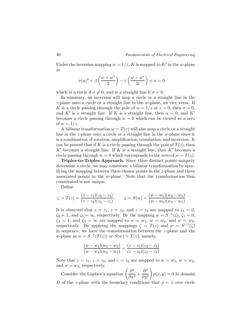
Under the inversion mapping w = 1/z, K is mapped to K ′ in the w-planeas

σ|w|2 + β

(w + w∗

2

)− γ

(w − w∗

2i

)+ α = 0

which is a circle if σ 6= 0, and is a straight line if σ = 0.In summary, an inversion will map a circle or a straight line in the

z-plane onto a circle or a straight line in the w-plane, an vice versa. IfK is a circle passing through the pole of w = 1/z at z = 0, then σ = 0,and K ′ is a straight line. If K is a straight line, then α = 0, and K ′

becomes a circle passing through w = 0 which can be viewed as a zeroof w = 1/z.

A bilinear transformation w = T (z) will also map a circle or a straightline in the z-plane onto a circle or a straight line in the w-plane since itis a combination of rotation, amplification, translation, and inversion. Itcan be proved that if K is a circle passing through the pole of T (z), thenK ′ becomes a straight line. If K is a straight line, then K ′ becomes acircle passing through w = 0 which corresponds to the zero of w = T (z).

Triples-to-Triples Approach. Since three distinct points uniquelydetermine a circle, we may constitute a bilinear transformation by spec-ifying the mapping between three chosen points in the z-plane and threeassociated points in the w-plane. Note that the transformation thusconstituted is not unique.

Define

ζ = T (z) =(z − z1)(z2 − z3)(z − z3)(z2 − z1)

, ζ = S(w) =(w − w1)(w2 − w3)(w − w3)(w2 − w1)

It is observed that z = z1, z = z2, and z = z3 are mapped to ζ1 = 0,ζ2 = 1, and ζ3 = ∞, respectively. By the mapping w = S−1(ζ), ζ1 = 0,ζ2 = 1, and ζ3 = ∞ are mapped to w = w1, w = w2, and w = w3,respectively. By applying the mappings ζ = T (z) and w = S−1(ζ)in sequence, we have the transformation between the z-plane and thew-plane as w = S−1(T (z)) or S(w) = T (z), namely,

(w − w1)(w2 − w3)(w − w3)(w2 − w1)

=(z − z1)(z2 − z3)(z − z3)(z2 − z1)

Note that z = z1, z = z2, and z = z3 are mapped to w = w1, w = w2,and w = w3, respectively.

Consider the Laplace’s equation

(∂2

∂x2+

∂2

∂y2

)p(x, y) = 0 in domain

D of the z-plane with the boundary conditions that p = 1 over circle

Complex Analysis 41

Figure 1.22. Conformal mapping by triples-to-triples approach.

K1 and p = 0 over circle K2 as shown in Fig.1.22. The more desirabledomain is shown as D′ of the w-plane. By arbitrarily mapping z = i,z = −1, and z = 1 to w = 0, w = 1, and w = ∞, respectively, we have(w − 0)(1−∞)(w −∞)(1− 0)

=(z − i)(−1− 1)(z − 1)(−1 − i)

, or w = (1− i)z − i

z − 1. The Laplace’s

equation is transformed to

(∂2

∂u2+

∂2

∂v2

)P (u, v) = 0 in D′ of the w-

plane, with the boundary conditions that P = 1 over the straight lineK ′

1 and P = 0 over the straight line K ′2. The imaginary part of the

analytic function w satisfies the required boundary conditions, namely,P = v is the solution in the w-plane. The solution in the z-plane canthus be derived as

p(x, y) = Im{w = T (z)} =1 − x2 − y2

(x − 1)2 + y2

The equipotential curve p(x, y) = c with constant c is a circle with theexplicit form of

(x − c

1 + c

)2

+ y2 =(

11 + c

)2

16. Schwarz-Christoffel TransformationThe Schwarz-Christoffel formula specifies a conformal mapping from

the upper half plane to a bounded or unbounded polygonal region. Con-sider the transformation w = (z − x1)α with 0 < α < 2 as shown inFig.1.23. Two colinear line segments zax1 and x1zb in the z-plane aremapped to two line segments waw1 and w1wb, respectively, with an inte-rior angle of απ. A differential in the w-plane is related to a differential


Figure 1.23. Conformal mapping by w = (z − x1)α.

in the z-plane by dw = α(z − x1)α−1dz. Hence, their arguments arerelated by Arg(dw) = (α − 1)Arg(z − x1) + Arg(dz). The directionalchange in the w-plane as z is moved from za via x1 to zb can be calcu-lated as Arg(dwb)−Arg(dwa) = (α− 1)[Arg(zb − x1)−Arg(za − x1)] +[Arg(dzb)−Arg(dza)] = (α− 1)(0− π) = (1− α)π, or the interior angleis απ.

By induction, a function of the formdw

dz= A

n∏

k=1

(z − xk)αk−1 will

map the real axis in the z-plane to a polygon in the w-plane, wherex1 < x2 < · · · < xn are n distinct points along the real axis in thez-plane, and 0 < αk < 2. Since the sum of all the directional changes asa point is moved along a polygon is equal to 2π, the {αk} must satisfy(1 − α1)π + · · ·+ (1 − αn)π = 2π or α1 + · · ·+ αn = n − 2. Thus, onlyn − 1 out of these {αk} can be chosen independently.

The mapping function can then be determined by integrating dw/dz =

f ′(z) over z to have f(z) = A

∫ n∏

k=1

(z − xk)αk−1dz + B, where A and

B are constants to be determined by the mapping of specific points.Sometimes, xn may be chosen at ∞, and the product contains only theterms with 1 ≤ k ≤ n − 1. Note that the transformation from the realaxis in the z-plane is not uniquely determined, one may map differentsets of {xk} to the same set of {wk}.

Consider the mapping shown in Fig.1.24 in which z1 = −1 and z2 = 1are mapped to w1 = −i and w2 = i, respectively. Both of the two interiorangles are π/2, hence α1 = α2 = 1/2, and f ′(z) = A(z+1)−1/2(z−1)−1/2.The mapping function can then be integrated as

f(z) = A

∫dz

(z2 − 1)1/2+ B = −Ai

∫dz

(1 − z2)1/2+ B = −Ai sin−1 z + B

By imposing f(−1) = −i and f(1) = i, we have A = −2/π and B = 0.Hence, the required mapping function is w = (2i/π) sin−1 z.

Next, consider the mapping shown in Fig.1.25 in which z1 = −1 andz2 = 0 are mapped to w1 = iπ and w2 = −∞, respectively. The two

Complex Analysis 43

Figure 1.24. Conformal mapping from real axis to half a rectilinear strip.

Figure 1.25. Conformal mapping from real axis to the real axis plus a semi-infiniteline.

interior angles are 2π and 0, respectively, or α1 = 2, α2 = 0. Hence,f ′(z) = A(z + 1)z−1. The mapping function can be integrated as

f(z) = A

∫z + 1

zdz + B = A(z + Lnz) + B

By imposing f(−1) = iπ and f(0) = −∞, we have A = B = 1. Hence,the required mapping function is w = (z + 1) + Lnz.

17. Poisson Integral FormulaConsider the solution to Laplace’s equation in the upper half plane

with boundary condition specified in Fig.1.26(a). It is observed thatp(x, y) = (pi/π)[Arg(z−b)−Arg(z−a)] is the solution since Arg(z−α)isthe imaginary part of the analytic function Ln(z−α), and p(x, y) satisfiesthe boundary condition over the real axis.


Figure 1.26. Harmonic function in the upper half plane: (a) step boundary condition,(b) piecewise constant boundary condition.

Next, consider the boundary condition specified in Fig.1.26(b). Thesolution can be obtained by extending the previous case to be

p(x, y) =n∑

k=1

pk

π[Arg(z − xk) − Arg(z − xk−1)]

=1π

n∑

k=1

∫ xk

xk−1

pkd

dtArg(z − t)dt

=1π

n∑

k=1

∫ xk

xk−1

pky

(x − t)2 + y2dt (1.23)

where Arg(z − t) = tan−1[y/(x− t)].A continuous function p(x, 0) specified over the real axis can be ap-

proximated by piecewise constants over infinitesimal intervals. Thus, thesolution (1.23) can be extended to the case where a continuous boundarycondition is specified over the real axis as

p(x, y) =y

π

∫ ∞

−∞

p(t, 0)(x − t)2 + y2

dt

Complex Analysis 45

References

[1] D. G. Zill and P. D. Shanahan, A First Course in Complex Analysiswith Applications, Jones and Bartlett Publishers, 2003.

[2] A. D. Wunsch, Complex Variables with Applications, 3rd ed., Pear-son Education, 2005.

[3] J. A. Stratton, Electromagnetic Theory, McGraw-Hill, 1941.

Documents

Chapter 1 COMPLEX ANALYSIS - 國立臺灣大學cc.ee.ntu.edu.tw/~jfkiang/complex analysis/complex_analysis.pdfChapter 1 COMPLEX ANALYSIS Jean-Fu Kiang Department of Electrical Engineering