Chapter 1Introduction

• What are longitudinal and panel data?• Benefits and drawbacks of longitudinal data• Longitudinal data models• Historical notes

1.1 What are longitudinal and panel data?• With regression data, we collect a cross-section of subjects.

– The interest is comparing characteristics of the subject, that is, investigating relationships among the variables.

• In contrast, with time series data, we identify one or more subjects and observe them over time.– This allows us to study relationships over time, the so-called

dynamic aspect of a problem.• Longitudinal/panel data represent a marriage of regression

and time series data.– As with regression, we collect a cross-section of subjects.– With panel data, we observe each subject over time.

• The descriptor panel data comes from surveys of individuals; a panel is a group of individuals surveyed repeatedly over time.

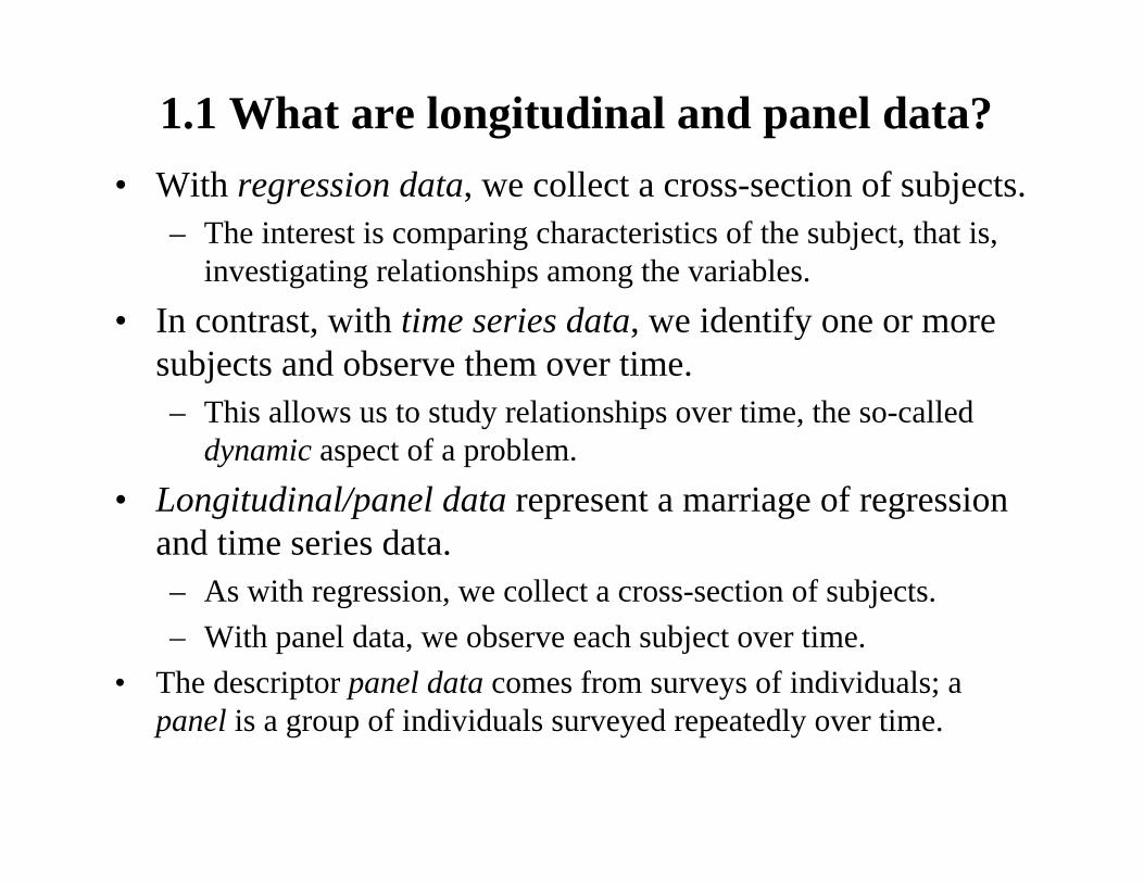
Example 1.1 - Divorce rates• Figure 1.1 shows the 1965 divorce rates versus AFDC (Aid

to Families with Dependent Children) for the fifty states.– The correlation is -0.37.– Counter-intuitive? - we might expect a positive relationship

between welfare payments (AFDC) and divorce rates.

20 120 220

0

1

2

3

4

5

AFDC Payments

DivorceRates

1965 Divorce Rates to AFDC Payments

Example 1.1 - Divorce rates• A similar figure shows a negative relationship for 1975 (the

correlation is -0.425)• Figure 1.2 shows both 1965 and 1975 data, with a line

connecting each state– The line represents a change over time (dynamic), not a

cross-sectional relationship.– Each line displays a positive relationship - as welfare

payments increase so do divorce rates.– This is not to argue for a causal relationship between

welfare payments and divorce rates.• The data are still observational.• The dynamic relationship between divorce and AFDC is

different from the cross-sectional relationship.

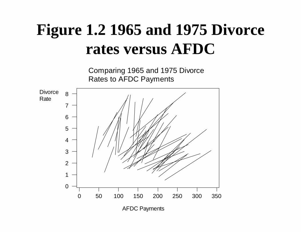
Figure 1.2 1965 and 1975 Divorce rates versus AFDC

0 50 100 150 200 250 300 350

0

1

2

3

4

5

6

7

8

AFDC Payments

DivorceRate

Comparing 1965 and 1975 DivorceRates to AFDC Payments

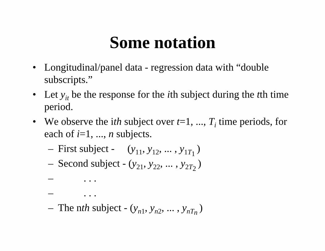
Some notation• Longitudinal/panel data - regression data with “double

subscripts.”• Let yit be the response for the ith subject during the tth time

period. • We observe the ith subject over t=1, ..., Ti time periods, for

each of i=1, ..., n subjects.– First subject - (y11, y12, ... , y1T1 )– Second subject - (y21, y22, ... , y2T2 )– . . .– . . . – The nth subject - (yn1, yn2, ... , ynTn )

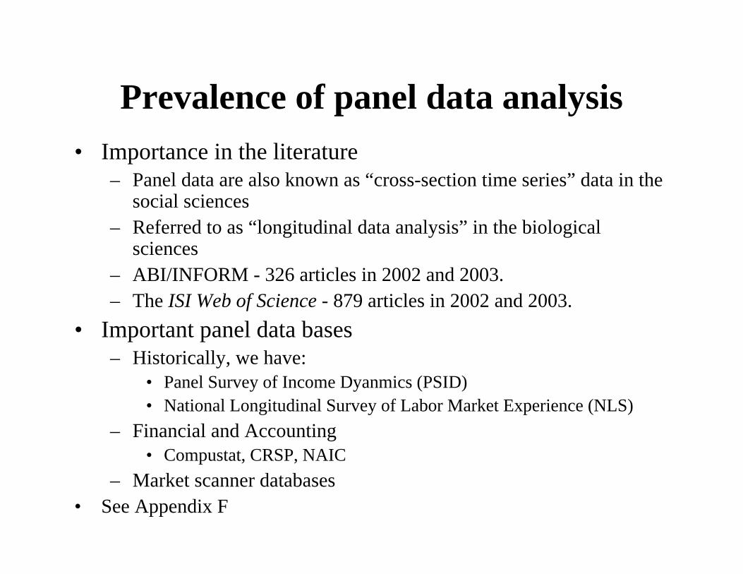
Prevalence of panel data analysis• Importance in the literature

– Panel data are also known as “cross-section time series” data in the social sciences

– Referred to as “longitudinal data analysis” in the biological sciences

– ABI/INFORM - 326 articles in 2002 and 2003.– The ISI Web of Science - 879 articles in 2002 and 2003.

• Important panel data bases– Historically, we have:

• Panel Survey of Income Dyanmics (PSID)• National Longitudinal Survey of Labor Market Experience (NLS)

– Financial and Accounting• Compustat, CRSP, NAIC

– Market scanner databases• See Appendix F

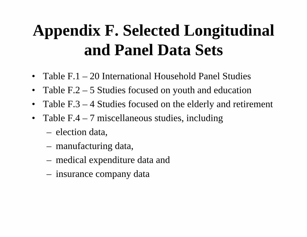
Appendix F. Selected Longitudinal and Panel Data Sets

• Table F.1 – 20 International Household Panel Studies• Table F.2 – 5 Studies focused on youth and education• Table F.3 – 4 Studies focused on the elderly and retirement• Table F.4 – 7 miscellaneous studies, including

– election data, – manufacturing data, – medical expenditure data and – insurance company data

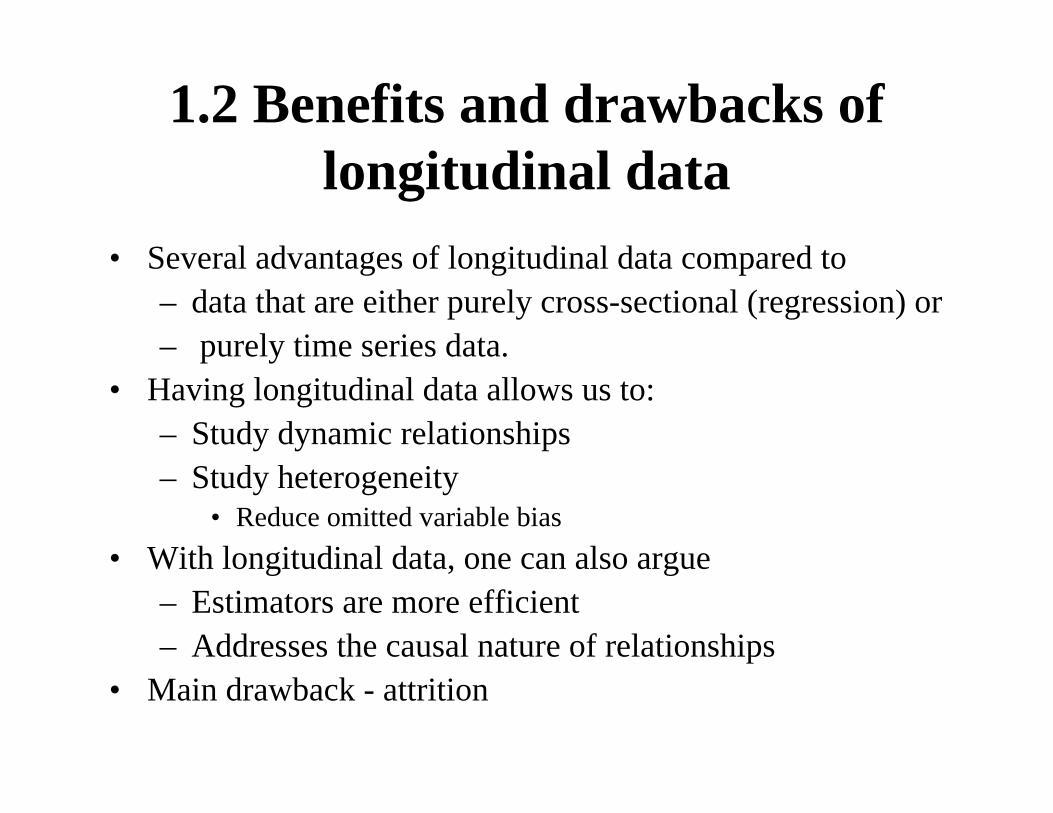
1.2 Benefits and drawbacks of longitudinal data

• Several advantages of longitudinal data compared to– data that are either purely cross-sectional (regression) or– purely time series data.

• Having longitudinal data allows us to:– Study dynamic relationships– Study heterogeneity

• Reduce omitted variable bias• With longitudinal data, one can also argue

– Estimators are more efficient– Addresses the causal nature of relationships

• Main drawback - attrition

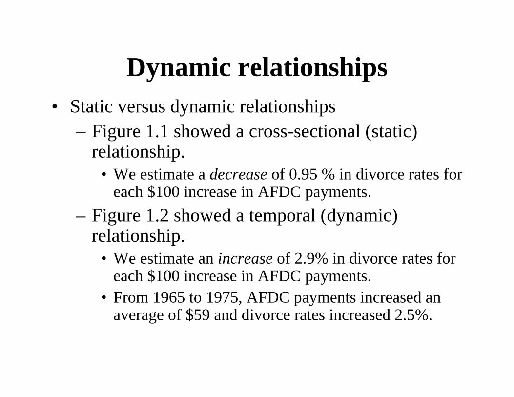
Dynamic relationships• Static versus dynamic relationships

– Figure 1.1 showed a cross-sectional (static) relationship.

• We estimate a decrease of 0.95 % in divorce rates for each $100 increase in AFDC payments.

– Figure 1.2 showed a temporal (dynamic) relationship.

• We estimate an increase of 2.9% in divorce rates for each $100 increase in AFDC payments.

• From 1965 to 1975, AFDC payments increased an average of $59 and divorce rates increased 2.5%.

Historical approach• In early panel data studies, pooled cross-sectional data were

analyzed by – estimating cross-sectional parameters using regression

and– using time series methods to model the regression

parameter estimates, treating the estimates as known with certainty.

• Theil and Goldberger (1961) provide an early discussion on the advantages of estimating these two aspects simultaneously.

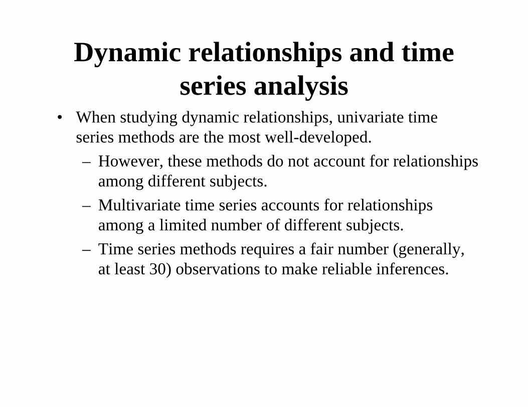
Dynamic relationships and time series analysis

• When studying dynamic relationships, univariate time series methods are the most well-developed.– However, these methods do not account for relationships

among different subjects.– Multivariate time series accounts for relationships

among a limited number of different subjects.– Time series methods requires a fair number (generally,

at least 30) observations to make reliable inferences.

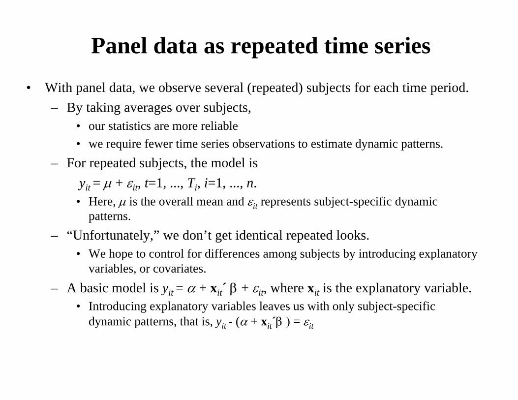
Panel data as repeated time series

• With panel data, we observe several (repeated) subjects for each time period.– By taking averages over subjects,

• our statistics are more reliable • we require fewer time series observations to estimate dynamic patterns.

– For repeated subjects, the model isyit = µ + εit, t=1, ..., Ti, i=1, ..., n. • Here, µ is the overall mean and εit represents subject-specific dynamic

patterns.– “Unfortunately,” we don’t get identical repeated looks.

• We hope to control for differences among subjects by introducing explanatory variables, or covariates.

– A basic model is yit = α + xit´ β + εit, where xit is the explanatory variable.• Introducing explanatory variables leaves us with only subject-specific

dynamic patterns, that is, yit - (α + xit´β ) = εit

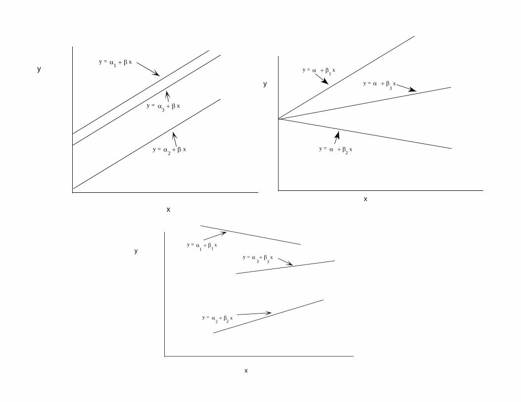
Heterogeneity• Subjects are unique.

– In cross-sectional analysis, we use yit = α + xit´β + εit• ascribe the uniqueness to " εit ".

– In panel data, we have an opportunity to model this uniqueness.– The model yit = αi + xit´β + εit is

• unidentifiable in cross-sectional regression. • In panel data, we can estimate β and α1, .., αn.

• Subject-specific parameters, such as αi, provide an important mechanism for controlling heterogeneity of individuals.

• Vocabulary: – When {αi} are fixed, unknown parameters to be estimated, we

call this a fixed effects model. – When {αi} are drawn from an unknown population, that is,

random variables, we call this a model with random effects.

Heterogeneity bias• Suppose that a data analyst mistakenly uses the model

yit = α + xit´β + εit

when yit = αi + xit´β + εit is the true model. – This is an example of heterogeneity bias, or a problem

with aggregation with data.• Similarly, one could have different (heterogeneous) slopes

yit = α + xit´βi + εit

• or different intercepts and slopesyit = αi + xit´βi + εit

y

x

α + βy = x1

α + βy = x3

α + βy = x2

y

x

α + βy = x1

α + βy = x3

α + βy = x2

1

3

2

y

x

α + βy = x1

α + βy = x3

α + βy = x2

Omitted variables• Panel data serves to reduce the omitted variable bias.• When omitted variables are time constant, we can still get

reliable estimates. • Consider the “true” model yit = α + xit´β + zi´γ + εit.

– Unfortunately, we cannot (or not thought to) measure zi.– It is “lurking” or “latent.” By considering the changes

yit* = yit - yi,t-1 = (α + xit´β + zi´γ + εit) - (α + xit-1´β + zi´γ + εit-1)

= (xit - xit -1 )´β + εit - εit-1) = xit* ´ β + εit

*

– we do not need to worry about the bias that ordinarily arises from the latent variable, zi .

• Introducing the subject-specific variable αi, accounts for the presence of many types of latent variables.

Efficiency of Estimators• Subject-specific variables αi also account for a large portion of

the variability in many data sets– This reduces the mean square error – Increases the efficiency (or reduces the standard errors) of

our parameter estimators.• With panel data, we generally have more observations than

with time series or regression. • A longitudinal data design may yield more efficient estimators

than estimators based on a comparable amount of data from alternative designs. – Suppose that the interest is in assessing the average change in a

response over time, such as the divorce rate. – A repeated cross-section yields– Longitudinal data design yields

( ) 2121 VarVarVar •••• +=− yyyy

( ) ( )212121 ,Cov2VarVarVar •••••• −+=− yyyyyy

Causality and correlation• Three ingredients necessary for establishing causality, taken

from the sociology literature:– A statistically significant relationship is required.– The association between two variables must not be due

to another, omitted, variable.– The “causal” variable must precede the other variable in

time.• Longitudinal data are based on measurements taken over

time and thus address the third requirement of a temporal ordering of events.

• Moreover, longitudinal data models provide additional strategies for accommodating omitted variables that are not available in purely cross-sectional data.

Drawbacks: Sampling Design (attrition)

• Selection bias – may occur when a rule other than simple random

sampling is used to select observational units– Example – “endogeneous” decisions by agents to join a

labor pool or participate in a social program.• Missing data

– Because we follow the same subjects over time, nonresponse typically increases through time.

– Example: US Panel Study of Income Dynamics (PSID):• In the first year (1968), the nonresponse rate was 24%.• By 1985, the nonresponse rate was about 50%.

1.3 Longitudinal data models• Types of inference

– Primary. We are interested in the effect that an (exogenous) explanatory variable has on a response, controlling for other variables (including omitted variables).

– Forecasting. We would like to predict future values of the response from a specific subject.

– Conditional means. • We would like to predict the expected value of a future

response from a specific subject. • Here, the conditioning is on latent (unobserved)

characteristics associated with the subject.• Types of applications - many

Social science statistical modeling• A model based on data characteristics is known as a

sampling based model. The model arises from a data generating process.

• In contrast, a structural model is a statistical model that represents causal relationships, as opposed to relationships that simply capture statistical associations.

• Why bother with an extra layer of theory when considering statistical models? Manski (1992) offers : – Interpretation - the primary purpose of many statistical analyses is

to assess relationships generated by theory from a scientific field. – Structural models utilize additional information from an underlying

functional field. If this information is utilized correctly, then in some sense the structural model should provide a better representation than a model without this information. (explanation)

– Particularly for public policy analysis, the goal of a statistical analysis is to infer the likely behavior of data outside of those realized (extrapolation).

Modeling issues• With subject-specific parameters, there can be many

parameters that describe the model– “Fixed” versus “random” effects models

• Incorporating dynamic structure is important– Econometric “dynamic” models (lagged endogenous)

versus serial correlation approach• Linear versus nonlinear (generalized linear) models

– Marginal versus hierarchical estimation approaches• Parametric versus semiparametric models• We wish to separate the effects of:

– the mean– the cross-sectional variance and– serial correlation structure

1.4 Historical notes• The term ‘panel study’ was coined in a marketing context

when Lazarsfeld and Fiske (1938)– Considered the effect of radio advertising on product sales. – People buy a product would be more likely to hear the

advertisement, or vice versa. – They proposed repeatedly interviewing a set of people (the ‘panel’)

to clarify the issue.• Econometrics

– Early economics applications include Kuh (1959), Johnson (1960),Mundlak (1961) and Hoch (1962).

• Biostatistics– Wishart (1938), Rao (1959, 1965), Potthoff and Roy (1964) – used

multivariate analysis to consider the problem of polynomial growth curves of serial measurements from a single group of subjects.

– Grizzle and Allen (1969) – introduced covariates