CHAPTER 9

APT AND MULTIFACTOR MODELS OF RISK AND RETURN

Arbitrage◦ Exploitation of security mispricing, risk-free

profits can be earned No arbitrage condition, equilibrium market

prices are rational in that they rule out arbitrage opportunities

9.1 MULTIFACTOR MODELS

Single Factor Model

Returns on a security come from two sources◦Common macro-economic factor◦Firm specific events

Focus directly on the ultimate sources of risk, such as risk assessment when measuring one’s exposures to particular sources of uncertainty

Factors models are tools that allow us to describe and quantify the different factors that affect the rate of return on a security

Single Factor Model

ri = Return for security I

= Factor sensitivity or factor loading or factor beta

F = Surprise in macro-economic factor(F could be positive, negative or zero)

ei = Firm specific events

F and ei have zero expected value, uncorrelated

( )i i i ir E r F e

i

Single Factor Model

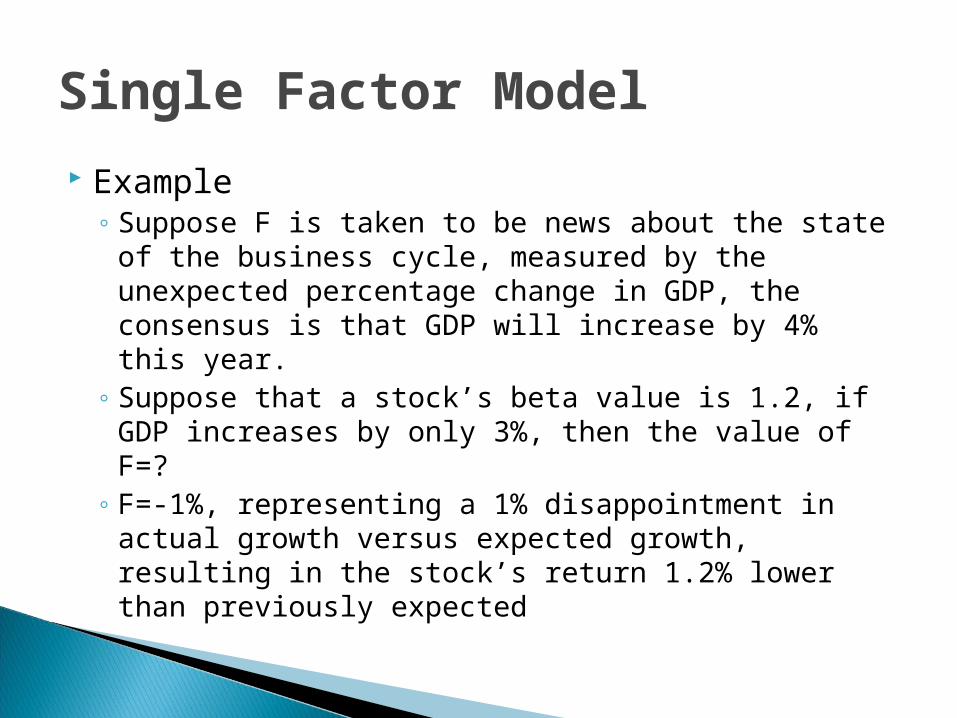
Example◦ Suppose F is taken to be news about the state of

the business cycle, measured by the unexpected percentage change in GDP, the consensus is that GDP will increase by 4% this year.

◦ Suppose that a stock’s beta value is 1.2, if GDP increases by only 3%, then the value of F=?

◦ F=-1%, representing a 1% disappointment in actual growth versus expected growth, resulting in the stock’s return 1.2% lower than previously expected

Multifactor Models

Macro factor summarized by the market return arises from a number of sources, a more explicit representation of systematic risk allowing for the possibility that different stocks exhibit different sensitivities to its various components◦ Use more than one factor in addition to market return

Examples include gross domestic product, expected inflation, interest rates etc.

Estimate a beta or factor loading for each factor using multiple regression.

Multifactor models, useful in risk management applications, to measure exposure to various macroeconomic risks, and to construct portfolios to hedge those risks

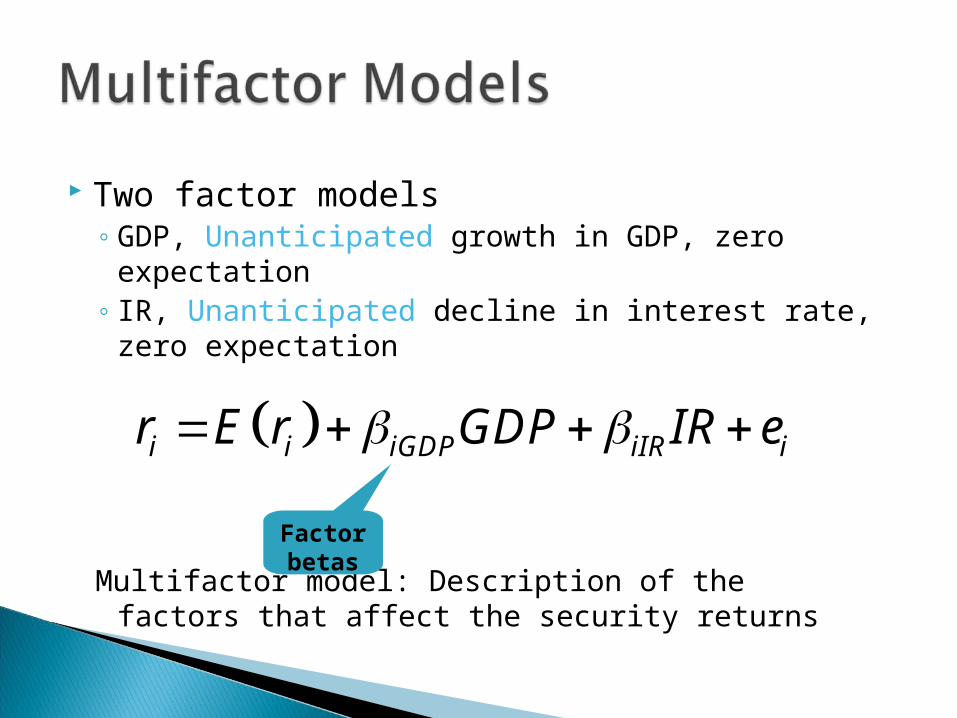
Two factor models◦ GDP, Unanticipated growth in GDP, zero

expectation◦ IR, Unanticipated decline in interest rate, zero

expectation

Multifactor model: Description of the factors that affect the security returns

i i iGDP iIR ir E r GDP IR e

Factor betas

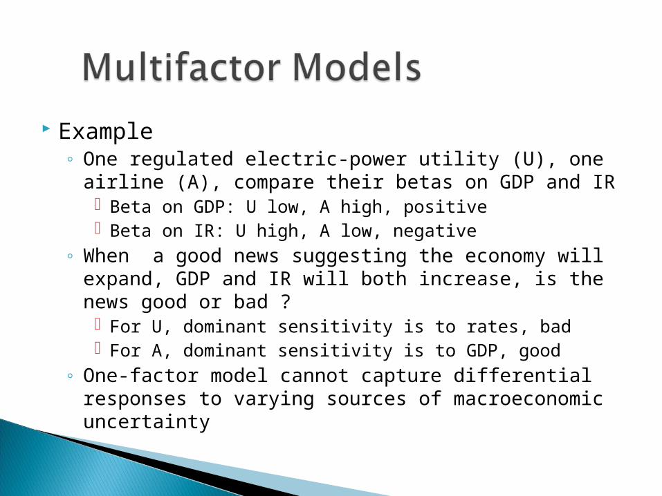
Example◦ One regulated electric-power utility (U), one airline

(A), compare their betas on GDP and IR Beta on GDP: U low, A high, positive Beta on IR: U high, A low, negative

◦ When a good news suggesting the economy will expand, GDP and IR will both increase, is the news good or bad ? For U, dominant sensitivity is to rates, bad For A, dominant sensitivity is to GDP, good

◦ One-factor model cannot capture differential responses to varying sources of macroeconomic uncertainty

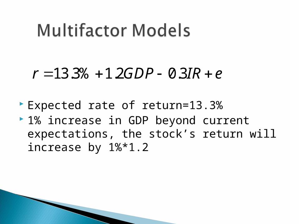
Expected rate of return=13.3% 1% increase in GDP beyond current

expectations, the stock’s return will increase by 1%*1.2

13.3% 1.2 0.3r GDP IR e

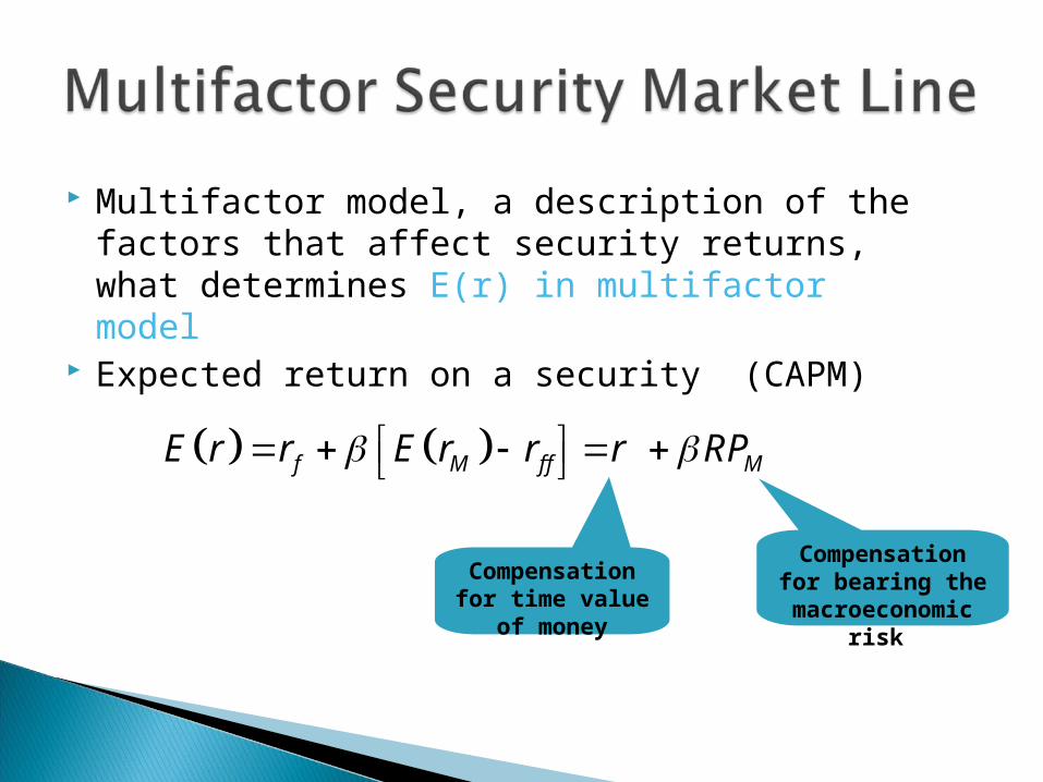
Multifactor model, a description of the factors that affect security returns, what determines E(r) in multifactor model

Expected return on a security (CAPM)

f M f f ME r r E r r r RP

Compensation for time value

of money

Compensation for bearing the macroeconomic

risk

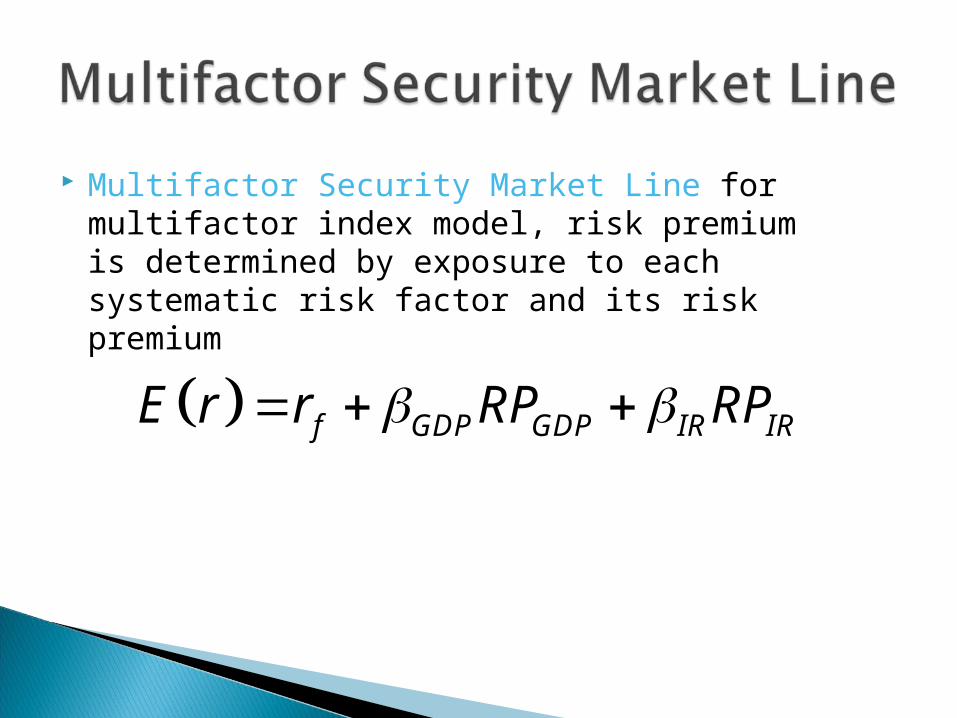
Multifactor Security Market Line for multifactor index model, risk premium is determined by exposure to each systematic risk factor and its risk premium

f GDP GDP IR IRE r r RP RP

9.2 ARBITRAGE PRICING THEORY

Stephen Ross, 1976, APT, link expected returns to risk

Three key propositions◦ Security returns can be described by a factor

model◦ Sufficient securities to diversify away idiosyncratic

risk◦ Well-functioning security markets do not allow for

the persistence of arbitrage opportunities

Arbitrage Pricing Theory

Arbitrage - arises if an investor can construct a zero investment portfolio with a sure profit

Since no investment is required, an investor can create large positions to secure large levels of profit

In efficient markets, profitable arbitrage opportunities will quickly disappear

Law of One Price◦ If two assets are equivalent in all economically

relevant respects, then they should have the same market price

Arbitrage activity◦ If two portfolios are mispriced, the investor could

buy the low-priced portfolio and sell the high-priced portfolio

◦ Market price will move up to rule out arbitrage opportunities

◦ Security prices should satisfy a no-arbitrage condition

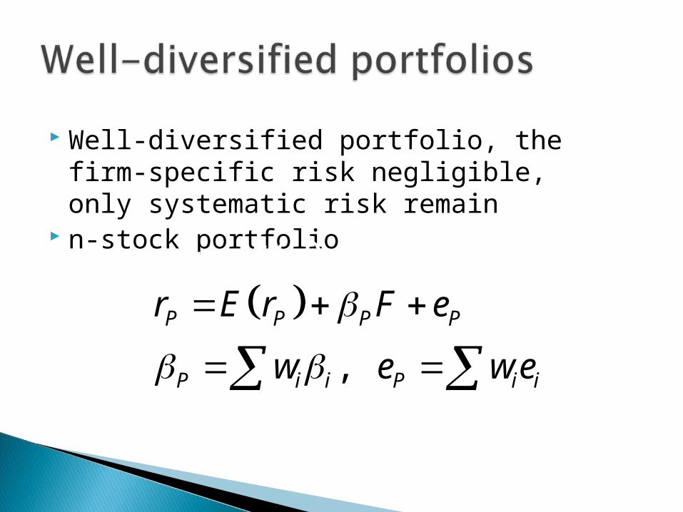
Well-diversified portfolio, the firm-specific risk negligible, only systematic risk remain

n-stock portfolio

,

P P P P

P i i P i i

r E r F e

w e we

i i i ir E r F e

The portfolio variance

If equally-weighted portfolio , the nonsystematic variance

N lager, the nonsystematic variance approaches zero, the effect of diversification

22

2 2 2 2

2

1 1var

1

i

P i i

i

ee i i i e e

e

iance w e wn n n

n

1iw n

2 2 2 2P P F ep

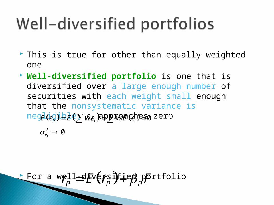
This is true for other than equally weighted one Well-diversified portfolio is one that is

diversified over a large enough number of securities with each weight small enough that the nonsystematic variance is negligible, eP approaches zero

For a well-diversified portfolio P P Pr E r F

2

0

0P

P i i i i

e

E e E we w E e

( )

( )i i i i

P P P P

r E r F e

r E r F e

Only systematic risk should command a risk premium in market equilibrium

Well-diversified portfolios with equal betas must have equal expected returns in market equilibrium, or arbitrage opportunities exist

Expected return on all well-diversified portfolio must lie on the straight line from the risk-free asset

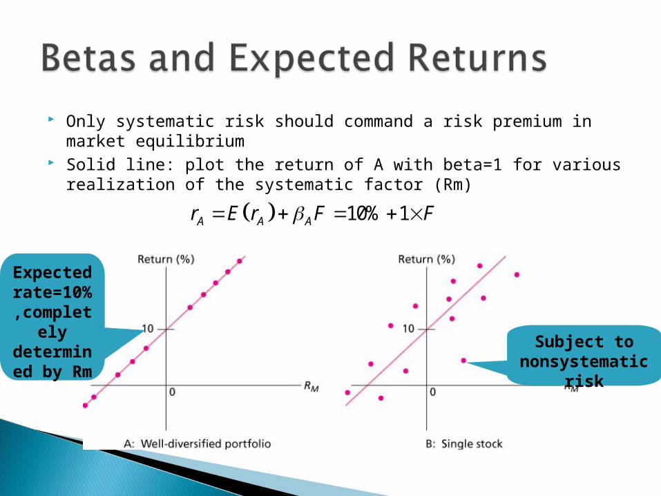
Only systematic risk should command a risk premium in market equilibrium

Solid line: plot the return of A with beta=1 for various realization of the systematic factor (Rm)

Expected

rate=10%,compl

etely determined by

Rm

Subject to nonsystemati

c risk

10% 1A A Ar E r F F

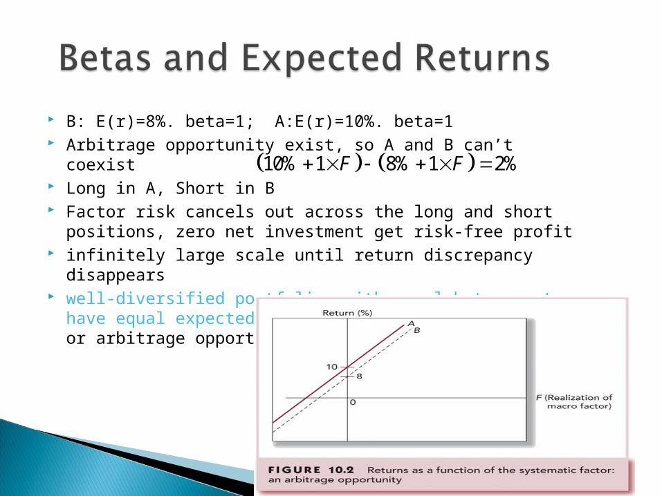
B: E(r)=8%. beta=1; A:E(r)=10%. beta=1 Arbitrage opportunity exist, so A and B can’t coexist Long in A, Short in B Factor risk cancels out across the long and short positions,

zero net investment get risk-free profit infinitely large scale until return discrepancy disappears well-diversified portfolios with equal betas must have equal

expected return in market equilibrium, or arbitrage opportunities exist

10% 1 8% 1 2%F F

What about different betas A: beta=1,E(r)=10%; C: beta=0.5,E(r)=6%; D: 50% A and 50% risk-free (4%) asset,

◦ beta=0.5*1+0.5*0=0.5, E(r)=7% C and D have same beta (0.5)

◦ different expected return◦ arbitrage opportunity

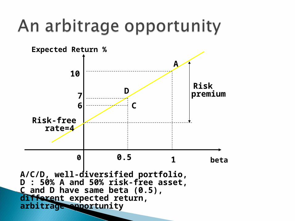
0.5*0 0.5*1 0.5

0.5*4% 0.5*10% 7%

Expected Return %

10

Risk-free rate=4

Risk premiu

m

0.5 beta 0 1

67

C

D

A

A/C/D, well-diversified portfolio, D : 50% A and 50% risk-free asset, C and D have same beta (0.5),different expected return,arbitrage opportunity

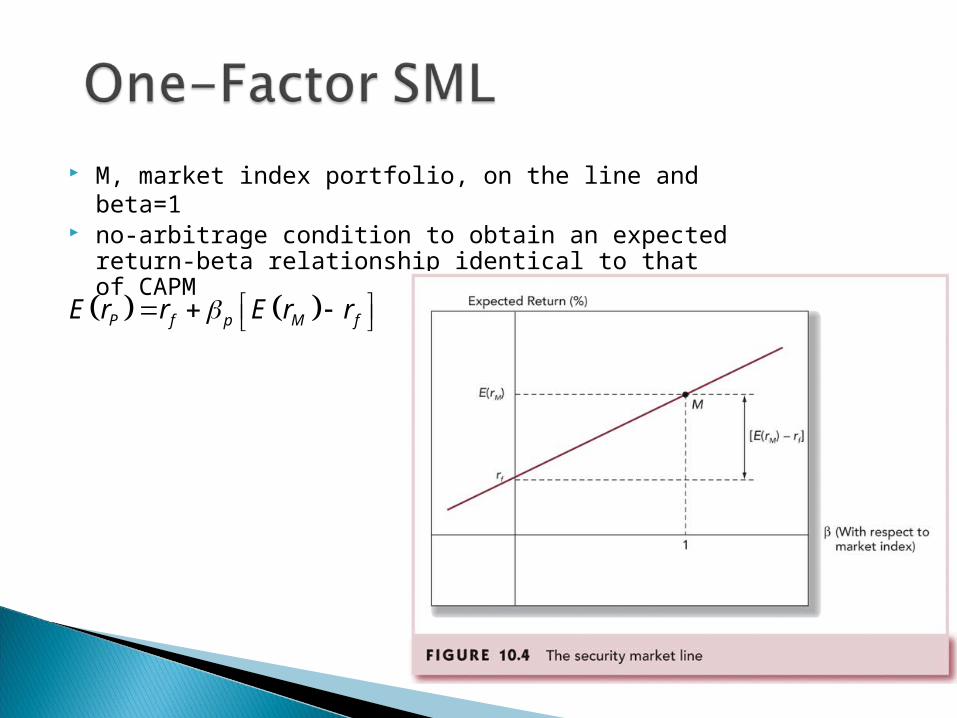
M, market index portfolio, on the line and beta=1 no-arbitrage condition to obtain an expected return-

beta relationship identical to that of CAPM

P f p M fE r r E r r

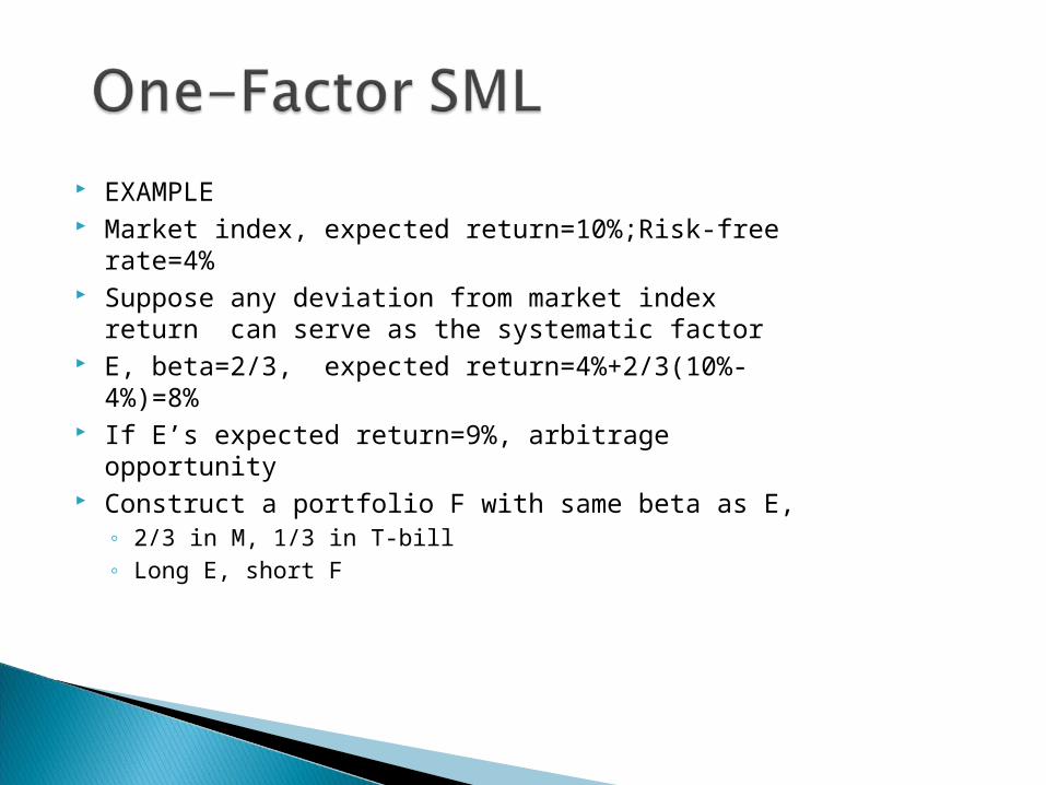
EXAMPLE Market index, expected return=10%;Risk-free

rate=4% Suppose any deviation from market index return can

serve as the systematic factor E, beta=2/3, expected return=4%+2/3(10%-

4%)=8% If E’s expected return=9%, arbitrage opportunity Construct a portfolio F with same beta as E,

◦ 2/3 in M, 1/3 in T-bill◦ Long E, short F

M, market index portfolio, as a well-diversified portfolio, no-arbitrage condition to obtain an expected return-beta relationship identical to that of CAPM

three assumptions: a factor model, sufficient number of securities to form a well-diversified portfolios, absence of arbitrage opportunities

APT does not require that the benchmark portfolio in SML be the true market portfolio

9.3 A MULTIFACTOR APT

Multifactor APT

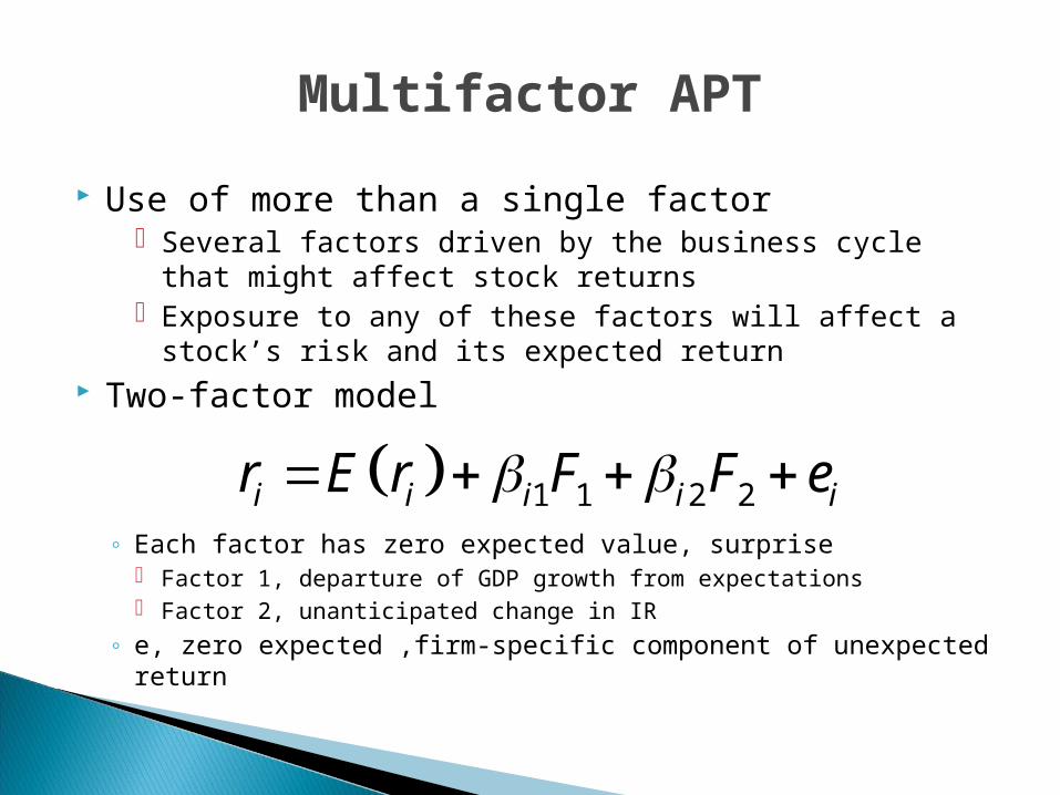
Use of more than a single factor Several factors driven by the business cycle that might

affect stock returns Exposure to any of these factors will affect a stock’s

risk and its expected return Two-factor model

◦ Each factor has zero expected value, surprise Factor 1, departure of GDP growth from expectations Factor 2, unanticipated change in IR

◦ e, zero expected ,firm-specific component of unexpected return

1 1 2 2i i i i ir E r F F e

Requires formation of factor portfolios◦ Factor portfolio:

Well-diversified Beta of 1 for one factor Beta of 0 for any other

◦ Or Tracking portfolio: the return on such portfolio track the evolution of particular sources of macroeconomic risk, but are uncorrelated with other sources of risk

◦ Factor portfolios will serve as the benchmark portfolios for a multifactor SML

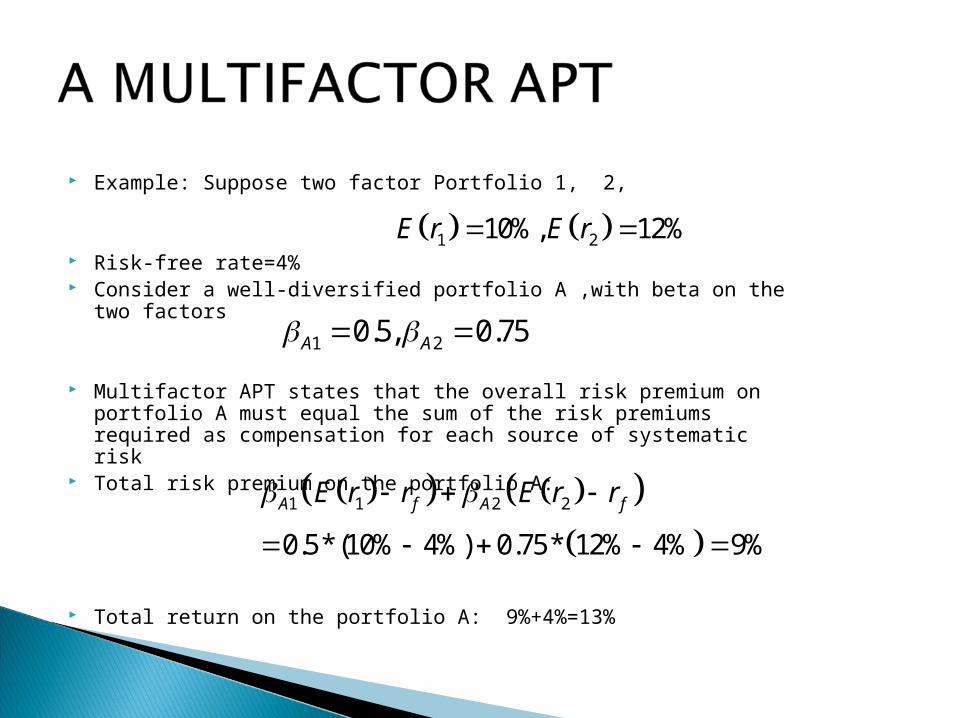
Example: Suppose two factor Portfolio 1, 2,

Risk-free rate=4% Consider a well-diversified portfolio A ,with beta on the two

factors

Multifactor APT states that the overall risk premium on portfolio A must equal the sum of the risk premiums required as compensation for each source of systematic risk

Total risk premium on the portfolio A:

Total return on the portfolio A: 9%+4%=13%

1 20.5, 0.75A A

1 1 2 2

0.5*(10% 4%) 0.75* 12% 4% 9%

A f A fE r r E r r

1 210%, 12%E r E r

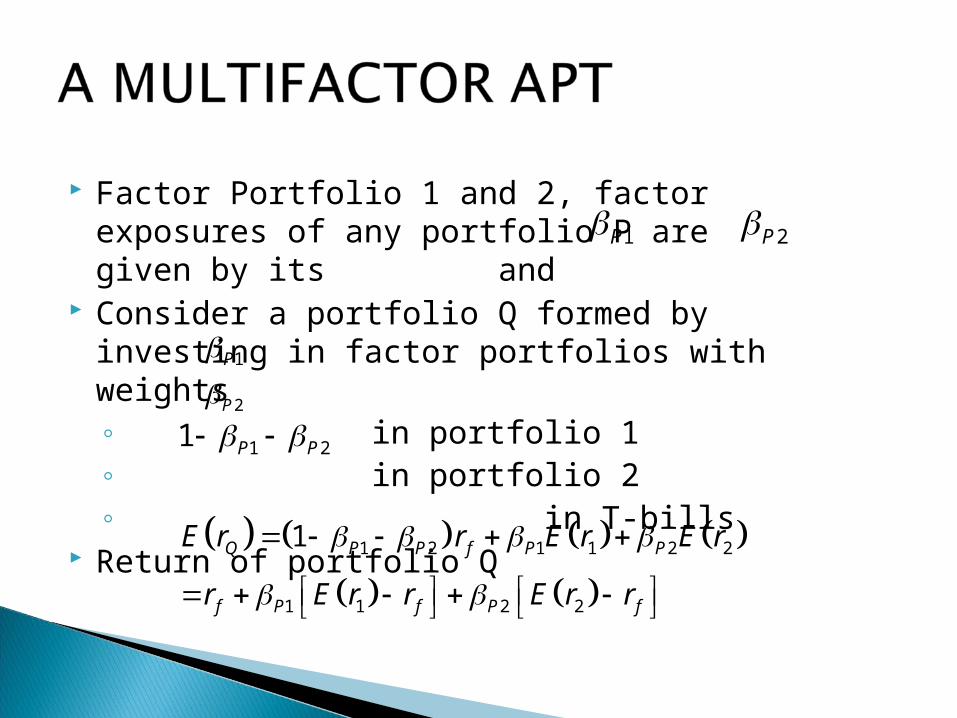
Factor Portfolio 1 and 2, factor exposures of any portfolio P are given by its and

Consider a portfolio Q formed by investing in factor portfolios with weights◦ in portfolio 1◦ in portfolio 2◦ in T-bills

Return of portfolio Q

1 2 1 1 2 2

1 1 2 2

1Q P P f P P

f P f P f

E r r E r E r

r E r r E r r

1P

2P

1 21 P P

1P 2P

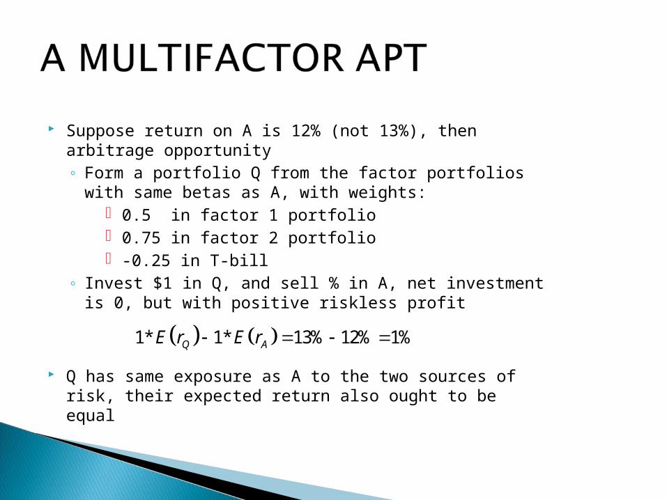
Suppose return on A is 12% (not 13%), then arbitrage opportunity◦ Form a portfolio Q from the factor portfolios with same

betas as A, with weights: 0.5 in factor 1 portfolio 0.75 in factor 2 portfolio -0.25 in T-bill

◦ Invest $1 in Q, and sell % in A, net investment is 0, but with positive riskless profit

Q has same exposure as A to the two sources of risk, their expected return also ought to be equal

1* 1* 13% 12% 1%Q AE r E r

9.4 WHERE TO LOOK FOR FACTORS

Multifactor APT

Two principles when specify a reasonable list of factors◦ Limit ourselves to systematic factors with considerable

ability to explain security returns◦ Choose factors that seem likely to be important risk

factors, demand meaningful risk premiums to bear exposure to those sources of risk

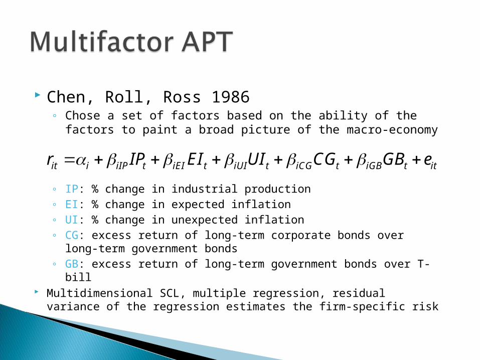
Chen, Roll, Ross 1986◦ Chose a set of factors based on the ability of the factors

to paint a broad picture of the macro-economy

◦ IP: % change in industrial production◦ EI: % change in expected inflation◦ UI: % change in unexpected inflation◦ CG: excess return of long-term corporate bonds over long-

term government bonds◦ GB: excess return of long-term government bonds over T-bill

Multidimensional SCL, multiple regression, residual variance of the regression estimates the firm-specific risk

it i iIP t iEI t iUI t iCG t iGB t itr IP EI UI CG GB e

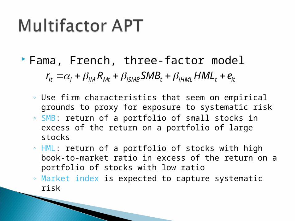
Fama, French, three-factor model

◦ Use firm characteristics that seem on empirical grounds to proxy for exposure to systematic risk

◦ SMB: return of a portfolio of small stocks in excess of the return on a portfolio of large stocks

◦ HML: return of a portfolio of stocks with high book-to-market ratio in excess of the return on a portfolio of stocks with low ratio

◦ Market index is expected to capture systematic risk

it i iM Mt iSMB t iHML t itr R SMB HML e

Fama, French, three-factor model◦ Long-standing observations that firm size and book-

to-market ratio predict deviations of average stock returns from levels with the CAPM

◦ High ratios of book-to-market value are more likely to be in financial distress, small stocks may be more sensitive to changes in business conditions

◦ The variables may capture sensitivity to risk-factors in macroeconomy

9.5 THE MULTIFACOTOR CAPM AND THE APT

Many of the same functions: give a benchmark for rate of return.

APT ◦ highlight the crucial distinction between factor risk

and diversifiable risk◦ APT assumption: rational equilibrium in capital

markets precludes arbitrage opportunities (not necessarily to individual stocks)

◦ APT yields expected return-beta relationship using a well-diversified portfolio (not a market portfolio)

APT and CAPM Compared

APT applies to well diversified portfolios and not necessarily to individual stocks

APT is more general in that it gets to an expected return and beta relationship without the assumption of the market portfolio

APT can be extended to multifactor models

The Multifactor CAPM and the APM

A multi-index CAPM ◦ Derived from a multi-period consideration of a stream of

consumption◦ will inherit its risk factors from sources of risk that a

broad group of investors deem important enough to hedge, from a particular hedging motive

The APT is largely silent on where to look for priced sources of risk