Chapter One

Understanding Animal Behavior

The subject of this book is animal behavior. What is animal behavior, and what does it mean to understand animal behavior? As we shall see in this chapter, there are several answers to these questions, depending on research tradition and what one intends to understand. At the same time, different theories of behavior have much the same scope:

• They deal with how the animal as a whole interacts with its physical, ecologi­cal and social environment, in particular through reception of sensory stimula­tion and behavioral actions such as motor patterns, pheromone release, change in body coloration and so forth.

• They want to explain, predict or control what animals do. • They consider situations in which internal factors such as memory and physi­

ological states are not easily accessible.

Besides our theoretical interests, there are great practical demands for knowledge of behavior. People who work with animals, such as zookeepers, farmers, animal trainers, veterinarians and conservationists, constantly need such knowledge.

Ethology and comparative psychology are two major research traditions dealing with behavior. Within these disciplines, it has been and still is important to ex­plore behavior as a function of external stimuli and readily observable factors such as species, age and sex. Internal factors such as physiological states and memory, on the other hand, are studied indirectly or inferred from observations of behavior, history of events and the passage of time. The reason for this difference is that in almost all situations in which we encounter animal behavior, it is relatively easy to monitor and control the external situation and to record behavior, but the access to internal factors is usually limited. However, ignoring internal factors undoubtedly has shortcomings. First, it is clear that external factors are not alone in causing behavior. An animal can react quite differently to the same piece of food, e.g., de­pending on hunger and memory of experiences with similar food items. Second, it is difficult to reconstruct behavior mechanisms from pure observations of behavior, and physiological knowledge about internal mechanisms may greatly facilitate the development of behavior models.

But what is the proper compromise between the complexity of nervous system and body physiology and the need for understanding at the behavioral level? The role of internal factors in models of behavior has been and still is a matter of much discussion. The most famous of these debates is the confrontation between be­haviorists, who attempted to avoid internal factors altogether, and cognitive psy­chologists, who instead encouraged theorizing about internal processes (Leahey

2 CHAPTER 1

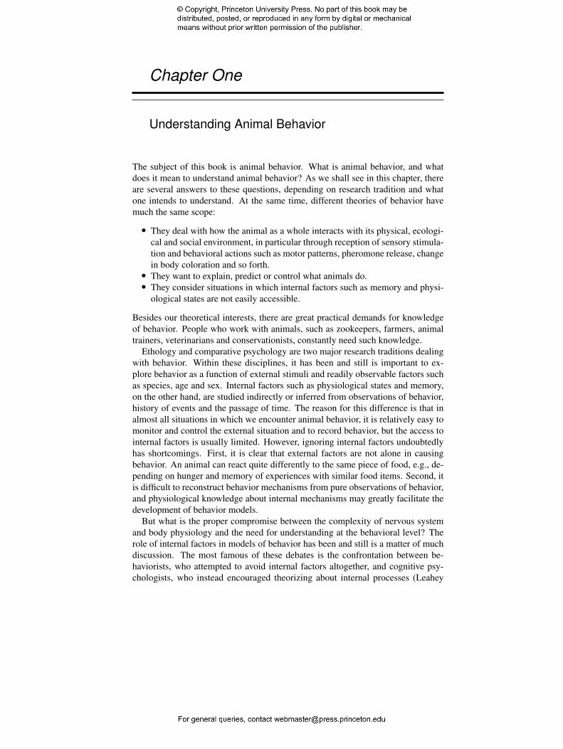
Figure 1.1 A newly hatched cuckoo chick dumps the eggs of its foster parents. The proxi­mate causes of this behavior are not the same as its ultimate causes. The proxi­mate explanation is that touch­sensitive receptors on the back of the chick elicit a behavior sequence that eventually results in eviction of the eggs. The ultimate, or evolutionary explanation is that chicks whose genes coded for this behavior survived better than chicks without such genes, since the former did not share the foster parents’ efforts with foster siblings. Reproduced from Davies (1992) by permission of artist David Quinn.

2004; Skinner 1985; Staddon 2001; see Section 1.3.5). We will discuss this issue at length in Chapter 6. In short, our position is that internal factors are vital for understanding behavior, but at the same time we side with behaviorists (and, of course, ethologists) in their focus on behavior and regard their contribution to the understanding of behavior as very significant.

In this chapter we first consider the different kinds of explanations that have been considered for behavior. We then introduce the reader to major theories of behav­ior, focusing on their structure and the causal factors invoked to explain behavior. Finally, we introduce neural networks models, which we will explore in this book as a potential framework for understanding behavior.

1.1 THE CAUSES OF BEHAVIOR

In biology, two types of causal explanations are generally recognized: proximate and ultimate explanations (Baker 1938; Mayr 1961). Proximate explanations ap­peal to motivational variables, experiences and genotype as the cause of behavior. Ultimate explanations refer to selection pressures and other factors that cause the evolution of behavior. These two kinds of causal explanations are independent and complementary, serving different purposes: one cannot replace the other. To clar­ify this concept, Lorenz (1981; §1.6) offers the following example. The ultimate

3 UNDERSTANDING ANIMAL BEHAVIOR

cause of cars is, of course, traveling. If the engine breaks, however, the ultimate cause cannot start it again: we need to know how the engine works (proximate causes). Figure 1.1 gives another example of this distinction, in the context of be­havior. Note that, in principle, we can learn independently about proximate and ultimate causes. However, the two are also related (since behavior is a result of evolution and influences evolution), and we probably will learn faster about one by also considering the other.

A more detailed set of explanations was suggested Niko Tinbergen in defining the scope of ethology (Tinbergen 1963). Rather than distinguishing just between proximate and ultimate causes, he argued that four questions must be answered to understand behavior. These are usually summarized as follows:

1. What causes a behavior to appear at a given moment and how does the be­havioral machinery work?

2. How does behavior develop during an individual’s lifetime? 3. What is the evolutionary history of the behavior? 4. How does the behavior contribute to survival and reproduction?

The first two questions are about the proximate explanation. Splitting it in two al­lows us to study behavior mechanisms at one time separately from how they change with time, an advantage on which we will capitalize. Tinbergen’s third question aims at a description of evolutionary change and does not refer to any causal ex­planation. The fourth question, as it is expressed, does not strictly refer to a causal explanation but to so­called final or functional explanations. These, with a leap of logic, invoke the effects of a behavior (contribution to survival and reproduction) as the cause of the behavior itself. In practice, however, the fourth question often covers true causal studies of the outcome of evolution, i.e., studies of how natural selection and other factors can modify behavior in an evolving population. Addi­tional discussion of explanations of animal behavior can be found in Alcock and Sherman (1994), Dewsbury (1992, 1999), and Hogan (1994a). In this book we consider three kinds of causal explanations closely related to Tinbergen’s:

1. Motivation 2. Ontogeny 3. Evolution

To us, understanding behavior means having answers to all of these questions, and this book is organized after this classification. The three explanations consider the causation of different phenomena and invoke different causes as follows.

A motivational explanation refers to individual behavior, and the goal is to pre­dict behavior from variables such as external stimulation and internal physiological states and to understand the behavior mechanism (Hogan 1994a). The term moti­vation refers to generally reversible and often short­term changes in behavior. An example is how animals use behavior to regulate food and water intake. Other examples include mechanisms of perception, decision making, motor control, etc. These topics are covered in Chapter 3.

Ontogeny refers to the development of the behavior mechanism during an in­dividual’s lifetime. The causes of ontogeny are the genotype and all the experi­

Very hungry

Hungry

Hungry and food available

Predator present

Look for food

Feed

Flee

Motivational states Behavioral repertoire

4 CHAPTER 1

Figure 1.2 An idealized behavior map associating motivational state (external and internal factors) with behavioral responses.

ences the individual has. The changes that occur include changes in the structure of the nervous system and memory changes, leading to generally long­term and less reversible changes in behavior (Hogan 1994a). Particular phenomena include learning, maturation, genetic predispositions and the development of the nervous system. Chapter 4 is dedicated to learning and other ontogenetic phenomena.

Lastly, evolution of behavior (or any other trait) occurs in a population of individ­uals and is manifested by changes in the population’s gene pool (Futuyma 1998). Causes of genetic changes include mutations, recombination, natural selection and chance. Selection may stem from the abiotic environment, from other species and from the behavior of conspecifics. These are the topics of Chapter 5. In species with culture, additional factors would have to be considered, but this is beyond the scope of this book.

1.2 A FRAMEWORK FOR MODELS OF BEHAVIOR

1.2.1 The behavior map: From motivational state to response

Central to this book and a starting point for most of our discussions is the assump­tion that behavior can be described and predicted based on knowledge about rele­vant motivational variables. These are simply the variables that enter motivational explanations of behavior. For instance, feeding behavior may be caused by the presence of food stimuli in combination with hunger, as illustrated in Figure 1.2. Research on behavior is partly about identifying motivational variables, and today, many are known, including physiological variables such as hormone levels and ex­ternal variables such as the shape and color of objects, the structure of mating calls, etc. The collection of all motivational variables at a given time is the animal’s mo­tivational state. A complete description of behavior assigns a behavioral response to each possible motivational state. Mathematically, we can express this notion

5 UNDERSTANDING ANIMAL BEHAVIOR

Table 1.1 How the behavior map enters different explanations of behavior.

Level of explanation

Motivation Ontogeny Evolution

Question What are the properties of How is the behavior How does evolution the behavior map? map determined? change behavior maps?

Causes External stimuli and Genes, experiences Environment (physical, internal states biological, social),

mutations, chance

Effects A behavioral response A behavior map Genetic code to develop a behavior map

Important Internal states of the body Memory and nervous Gene frequencies states and nervous system system connectivity and genotypes

with a function m that establishes a mapping from the set of motivational states X to the set of responses R. The latter contains the behavioral repertoire and other responses, such as hormone secretion. If we use x and r to refer to a single state and response, respectively, we can write

r = m(x) (1.1)

We will refer to m as the behavior map. This expression may sound technical, but it actually refers to something familiar to all students of behavior. For instance, the concepts of stimulus­response relationship, decision rule or response gradient are all examples of behavior maps. That is, they can be all written in the form of equa­tion (1.1) with appropriate choices of the input and output spaces and of the map function m. We use the expression behavior map for several reasons. First, it is not linked to any modeling tradition, but we can identify a behavior map in all theories of behavior. Second, the concept of a behavior map provides a sharp definition of what we mean by “understanding behavior” at different levels of explanation (Table 1.1). Third, our book explores neural networks as behavior maps.

The behavior map may be stochastic rather than deterministic. This means that a probability is assigned to each possible behavioral response rather than predicting exactly which one will occur. Whether true stochasticity occurs in behavior is a largely an unresolved problem (see, e.g., Dawkins & Dawkins 1974). Rather than attempting to solve this difficult issue, we note that stochastic factors may be included in the formalism above. For instance, we can include motivational variables that vary at random (Chapter 3).

1.2.2 The state­transition equation: Changes in motivational state

In addition to knowledge of the behavior map, if we want to predict sequences of behavior, we also need to know how the motivational state changes with time. Such changes may reflect changes in the environment (e.g., in the availability of a given food source) or changes within the animal (e.g., altered hormone levels). This book

6 CHAPTER 1

studies the impact of both external and internal factors. However, with respect to state changes, we are mainly interested in changes within the animal: first, because they are caused by processes in the animal whereas most changes to external states occur independent of the individual; and, second, because internal states allow the animal to organize its behavior in time and to detect temporal patterns in sensory input (Chapter 3).

Formally, changes in state can be described by means of equations of the form

x(t + 1) = M(x(t), r(t)) (1.2)

This equation simply says that the state at time t + 1 is a function of the state at time t and of the response of the system at time t (discrete rather than continuous time is considered for simplicity). In systems theory (Metz 1977; Minsky 1969), equation (1.2) is known as a state­transition equation, whereas equation (1.1) is the system’s response function, or output function. Examples of state­transition equations will be seen below, as well as in later chapters.

1.2.3 The behavior map in ontogeny and evolution

In summary, motivational explanations consider the properties of a particular be­havior map, i.e., how behavioral responses are caused by motivational states. A full understanding of motivational process also requires an understanding of mo­tivational state transitions. Ontogenetic and evolutionary explanations of behavior deal with different causes and effects.

In ontogenetic explanations, the effect is a behavior map, and the causes are an individual’s genes and experiences. Thus ontogeny considers how the map devel­ops and changes during an individuals life. It also covers the nature­nurture issue. One can express mathematically the behavior map as a function of the genotype g and the history of experiences h:

m = f (g, h) (1.3)

However, we prefer an approach based on state. An animal does not store its en­tire history; instead, its experiences result in a change to state variables W that determine the properties of the behavior map. Formally, we can write

m = f (W ) (1.4)

Most models of ontogeny and learning, including those based on neural networks, are of this kind. Note that the state variables of ontogenetic process are different from those of motivational process. The most obvious state variable in ontogeny is memory, and learning is a key mechanism for memory changes (memory state transitions). The state transition equation may be complex and depend on current state, genotype, motivational state and response.

Finally, to understand the genetic evolution of behavior, we have to consider evolutionary dynamics and a new class of state variables: the genes. Changes in gene frequencies and genotypes g are caused by the physical, ecological and social environment, as well as by mutations and other mechanisms that generate new genotypes. Evolution does not change the behavior map directly: the effect of genetic evolution is rather a genetic program for developing a behavior map.

7 UNDERSTANDING ANIMAL BEHAVIOR

1.2.4 Requirements on models of behavior

In summary, to understand behavior we need ways of describing behavior maps and state­transition equations. Ideally, models of behavior should fulfill the following requirements:

• Versatility: We observe great diversity in behavior both between species and, on a less dramatic scale, within species. The basic structure of a general model of behavior should allow for a diversity of behavior maps to be formed.

• Robustness: Regardless what explanation we seek, the mechanisms should display some robustness; otherwise, behavior would be vulnerable to any ge­netic or environmental disturbance. Thus small disturbances should not cause any major changes in performance.

• Learning: Learning from experience is a general feature of animal behavior. The model should allow learning, which should integrate realistically with the behavior map.

• Ontogeny: The behavior system of an individual develops in a sequence of events in which genes, the developing individual and the environment interact. The structure of the model should allow for gradual development of a behavior map from scratch to an adult form.

• Evolution: For evolution to occur, genetic variation must exist that affects the development of behavior mechanisms. In a model, it should be possible to specify how genes control features of behavior maps and learning mech­anisms. In addition, a model should allow the evolution of nervous systems from very simple forms to the complexities seen in, e.g., birds and mammals.

1.3 THE STRUCTURE OF BEHAVIOR MODELS

A diversity of behavior models exists, often developed for particular purposes such as the study of learning or perception. Important contributions to animal behavior theory come from the ethological tradition (McFarland 1974a; McFarland & Hous­ton 1981; Simmons & Young 1999) and from comparative psychology (Mackintosh 1994) but also from neuroscience (Cacioppo et al. 2000; Gazzaniga 2000; Kandel et al. 2000) and computer science (Wilson & Keil 1999). Here we consider dif­ferent modeling traditions from the point of view of model structure. By structure we simply mean the basic machinery of the model, e.g., how a motivational model generates the response from motivational variables. So far we have not provided any structures to the models we have considered. Adding structure to a model of behavior includes making assumptions about features of real animals, such as sense organs, central processes, memory, motor control and what are the available responses. What this means in practice will become clear in the following.

1.3.1 Operational and physiological models

What structure we need depends, of course, on our aims. We may distinguish roughly between operational and physiological models. An operational model aims

8 CHAPTER 1

to describe behavior realistically, but its structure is not intended to resemble the internal structure of animals. Such models are often referred to as black­box models to indicate lack of concern about underlying mechanisms. A physiological model, on the other hand, attempts to take into account more of the physiology that pro­duces behavior, e.g., body and nervous system physiology.

As will become clear in the following, the majority of models, both of human and of animal behavior, are operational models. Operational models are easier to build because only input­output relationships need to be described accurately and because we have fewer constraints on how to achieve such relationships. For instance, we may use the latest computer algorithm for pattern recognition instead of figuring out how a bunch of interconnected neurons can recognize anything. This is legitimate so long as we do not claim that agreement with observations implies identity of internal structure. Another factor favoring operational models is that physiology is more difficult to observe or control compared with behavior.

A crucial difference between physiological and operational models, and indeed the whole point in distinguishing them, is that the structure of physiological mod­els is not inferred solely from behavioral observations but is at least partly based on knowledge of physiology. There are several motives for doing this. One is to understand the neurophysiology of behavior. Another is the belief that a physio­logical model can be a more accurate behavioral model because its structure more closely mirrors the internal structure of animals.

In the following we consider the structure of behavior models from major re­search traditions, i.e., what behavior maps and state equations are used. We also discuss the extent to which models are operational or physiological. This will al­low us, throughout this book, to compare neural networks with other modeling traditions, highlighting differences and similarities.

1.3.2 Models with little or no structure

Some models of behavior make few assumptions about internal structure, allowing any input­output relationship to be formed with equal ease. Such unconstrained models have been used mainly for descriptive purposes and in studies of the evo­lution of behavior. A simple way of creating an unconstrained behavior map is to arrange motivational factors and behavioral responses in a look­up table, where each entry represents a particular input, and the content of the entry represents the behavioral output (Figure 1.3). It is possible to consider histories of events by in­cluding one table entry for each possible history (including the current situation). Thus a look­up table can cover learning, but not in its usual sense of changing stimulus­response relationships or memory. Rather, the effect of a particular indi­vidual history is to read out from the table one response instead of another.

One way to describe more explicitly sequences of events is to arrange them in a tree structure. As time unfolds, one progresses along the tree, following one branch or another depending on what decisions are taken. Such tree models can describe histories of experiences and allow for a unique responses to each history. A particular kind of tree model has been developed within game theory, referred to as the extensive­form description of a game (Figure 1.4; Fudenberg & Tirole

UNDERSTANDING ANIMAL BEHAVIOR 9

Motivational state Behavior response

Hungry Very hungry

Hungry + food available Predator present

. . .

Look for food Look for food

Feed Flee . . .

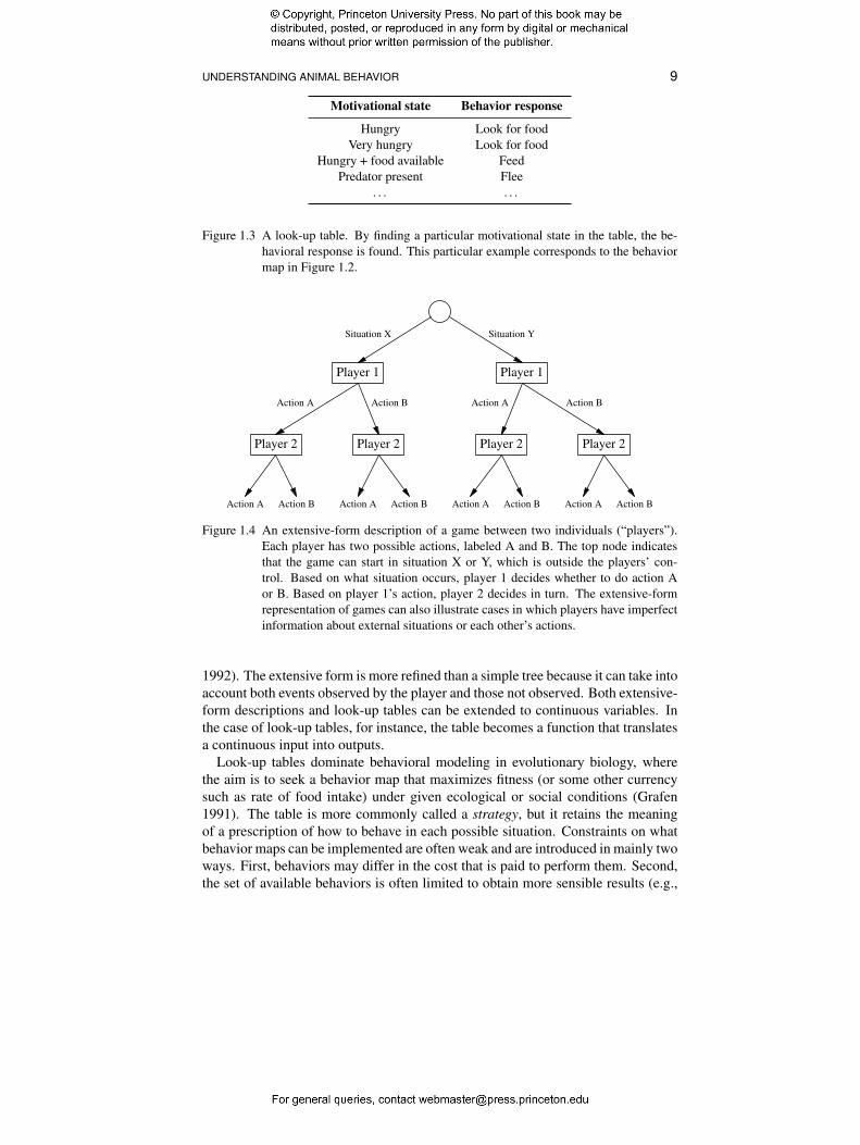
Figure 1.3 A look­up table. By finding a particular motivational state in the table, the be­havioral response is found. This particular example corresponds to the behavior map in Figure 1.2.

Player 1 Player 1

Situation X Situation Y

Player 2 Player 2 Player 2 Player 2

Action A

Action A Action B

Action B

Action A Action B

Action A

Action A Action B

Action B

Action A Action B

Figure 1.4 An extensive­form description of a game between two individuals (“players”). Each player has two possible actions, labeled A and B. The top node indicates that the game can start in situation X or Y, which is outside the players’ con­trol. Based on what situation occurs, player 1 decides whether to do action A or B. Based on player 1’s action, player 2 decides in turn. The extensive­form representation of games can also illustrate cases in which players have imperfect information about external situations or each other’s actions.

1992). The extensive form is more refined than a simple tree because it can take into account both events observed by the player and those not observed. Both extensive­form descriptions and look­up tables can be extended to continuous variables. In the case of look­up tables, for instance, the table becomes a function that translates a continuous input into outputs.

Look­up tables dominate behavioral modeling in evolutionary biology, where the aim is to seek a behavior map that maximizes fitness (or some other currency such as rate of food intake) under given ecological or social conditions (Grafen 1991). The table is more commonly called a strategy, but it retains the meaning of a prescription of how to behave in each possible situation. Constraints on what behavior maps can be implemented are often weak and are introduced in mainly two ways. First, behaviors may differ in the cost that is paid to perform them. Second, the set of available behaviors is often limited to obtain more sensible results (e.g.,

10 CHAPTER 1

a maximum running speed of preys and predators may be assumed). However, it is still true that all behavior maps, among those allowed, are assumed equally easy to form (e.g., Kamil 1998).

Models with no structure offer complete flexibility but have also drawbacks. First, they offer no insight into mechanisms of behavior. Second, each response is set independently of others. Thus there is no a priori reason why responses to similar inputs should yield similar outputs. For the same reason, responding in novel situations is undetermined, because the corresponding entry does not exist in the look­up table. In contrast, animal behavior exhibits clear regularities as a function of similarity between stimuli or situations (Section 3.3). Models without structure are unrealistic also because storing the response to each possible history of events requires an enormous memory. Of course, animals do not recall their entire history when deciding what to do. Instead, their behavior mechanism goes through successive changes of state, and the current state depends partly on the history of events. A last drawback of these models is that each table entry must be programmed genetically because there is no place for learning. We will return to these issues several times in this book, particularly in Chapter 5 on evolution.

1.3.3 Behavior as a function of motivational state

In this section we consider models that attempt to predict behavior based on a lim­ited number of motivational variables. The majority of motivational models are of this kind (e.g., Bolles 1975; McFarland 1971; McFarland & Houston 1981; Metz 1977). Motivational variables generally are categorized as either external stimuli (input to the system) or internal factors (system state variables). External stimu­lation can vary in many ways: different sense organs may be stimulated and each in many different ways. Examples of internal factors are water balance, hormone levels and memory. We shall elaborate on this distinction in Chapter 3.

Relevant motivational variables typically are identified from observations of be­havior, often combined with functional considerations (e.g., that body temperature must be maintained within limits for life to continue). The motivation state may also be identified from the animal’s recent history (e.g., hunger increases with the time since the last meal; Bolles 1975). Sometimes causal factors are induced from statistical analysis of observed data (Heiligenberg 1974; Wiepkema 1961) or by in­voking physiological considerations. For instance, models of feeding and drinking may consider stretch receptors in the stomach, water uptake rates from the stomach and receptors that monitor cellular water levels in the blood or elsewhere in the body (McFarland & Baher 1968; Toates 1986, 1998). The concept of state, includ­ing motivational state, today plays an important role also in evolutionary theory of animal behavior (Houston & McNamara 1999).

Given that relevant variables have been identified, the next question is how to combine them in a model of behavior. This is the issue of structure. A simple and classical example of a mathematically defined behavior map is given by summa­tion models of stimulus control. These attempt to predict the reaction to a com­pound stimulus from knowledge of reactions to its components in isolation. For a compound made up of three stimuli, for instance, the model can be formalized as

11 UNDERSTANDING ANIMAL BEHAVIOR

Figure 1.5 Interaction of internal and external factors in eliciting courtship behavior in male guppies (Lebistes reticulatus). The external factor is the size of a female dummy (vertical axis), whereas the internal factor is readiness to mate, as inferred from male coloration. The three curves represent the induction of three different com­ponents of courtship (pursuit of the female and two intensities of bending the body). From Baerends et al. (1955).

follows. To describe which stimuli are present, we introduce the motivational state x = (x1, x2, x3), with xi = 1 if stimulus i is present and 0 otherwise. We then define responding to the compound stimulus as the sum of the effects of its component:

r = W1x1 +W2x2 +W3x3 (1.5)

where Wi is the response to stimulus i. Only present stimuli influence responding, since xi = 0 for absent ones. Note the separation between state variables, which describe which stimuli are present, and the model structure, which describes how to obtain the response from the state, i.e., through a weighted sum. Models with this structure are the so­called law of stimulus summation (Leong 1969; Lorenz 1981; Seitz 1940–1941, 1943; Tinbergen 1951) and psychological models such as Rescorla and Wagner (1972) and Blough (1975). Note that some of the xi’s could be made to represent internal factors. In the latter case, external and internal factors would combine additively to produce the response. Of course, there are other ways in which factors can be combined (Figure 1.5; Krantz & Tversky 1971; McFarland & Houston 1981), and individual xi’s may not just take values of 0 and 1.

Another important theoretical concept is that of thresholds. Consider first the issue of whether to perform a given behavior or not based on the value of a single motivational variable, e.g., whether to eat or not for a given hunger level. A com­mon idea is that the behavior is performed if the motivational variable exceeds a threshold value T . Thresholds can also be applied to a combination of state vari­ables such as the weighted sum in equation (1.5). That is, a response to a given

12 CHAPTER 1

stimulus situation is assumed to occur if W1x1 +W2x2 +W3x3 > T (1.6)

A more complex situation occurs when incompatible responses are motivated si­multaneously (Ludlow 1980, 1976; McFarland 1989; McFarland & Sibly 1975). For instance, a hungry and thirsty animal cannot drink and eat at the same time. Usually, different behaviors or behavioral subsystems are assumed to “compete,” which means that the animal will show the behavior corresponding to the highest motivation (McFarland 1999).

The concept of thresholds and decision making can be generalized to decision boundaries in motivational state space. The motivational state x of the organism is represented as a point in a multidimensional state space, and to each point one response is assigned. Different regions in the space then are defined by setting decision boundaries. States within the same region yield the same behavior, but crossing a decision boundary leads to a change in behavior (McFarland 1999; Mc­Farland & Houston 1981).

To understand how behavior sequences are generated, we also need to consider how motivational state changes because the updated state will determine the subse­quent responses (McFarland 1971). This is a complex problem that operates at var­ious levels and time scales. Early theory of motivational state transitions was based on the drive concept (Hinde 1970). Each behavior was assumed to be controlled by a single internal factor (“drive”) that builds up with time and is reset to a low value each time the behavior is elicited. Since then, a diversity of state­transition mechanisms has been identified, and pure drives are probably rare. Modeling of motivational state­transitions and behavior sequences have benefited largely from applications of control theory and systems theory, yielding the most refined ap­proach to date for modeling motivational processes (McFarland 1971; Metz 1977; Toates 1998; Toates & Halliday 1980). An important concept is that of feedback mechanisms (McFarland 1971; Toates 1998). Many behavioral processes can be regarded naturally as controlling internal as well as external variables important for survival and reproduction. For instance, a lizard may use behavior to regulate its body temperature by moving between warmer and colder places within its territory. Feedback allows systems to respond to state changes brought about by previous ac­tions or the environment. Figure 1.6 depicts two block diagrams of mechanisms for motor control, one without a feed back loop and one with such a loop.

However, control of behavior is not limited to feedback from consequences of behavior. Within animals, many state variables have been identified that participate in the generation of behavior sequences. How such states change depends very much on their nature and may involve processes intrinsic to the nervous system (e.g., internal clocks), physiological states and processes outside the nervous sys­tem (e.g., hormones, water and energy status) and perceived external events and circumstances (e.g., social stimuli) or any combinations of these categories.

1.3.3.1 Summary

The concept of motivational state has proved useful, and models based on such a concept have been remarkably successful. An important contribution has been the

13 UNDERSTANDING ANIMAL BEHAVIOR

Eye position control

Control

centre

Extraocular muscle

control system

Motor

outflowEyeball ∑

Load

Position

Limb position control

Control

centre

Limb muscle

control system

Motor

outflowLimb ∑

Load

Position

Joint receptors

Figure 1.6 Outline of the eyeball and limb position­control systems illustrating the two prin­ciples of open­loop and closed­loop control. The feedback loop in the limb con­trol system allows correction of any deviation of the limb from the intended position. Reprinted by permission from McFarland (1971).

establishment that behavior systems can be regarded as dynamical systems (McFar­land 1971; McFarland & Houston 1981; Metz 1977) by complementing the equa­tion that describes the behavior map (output function) with state­transition equa­tions that update the motivational state (Houston & McNamara 1999; McFarland & Houston 1981). At least as they are applied today, however, models based on motivational state also have some weaknesses. First, applications of control theory to animal behavior have seldom considered learning (although learning to control is possible, see Sutton & Barto 1998; Widrow & Stearns 1985). Second, motivational factors are inferred from behavioral observations and sometimes from knowledge about body physiology, but the structure of the models is inferred from behav­ioral observations only. The concept of response threshold, for instance, has been criticized, and it remains unclear whether it can describe animal decision making satisfactorily (Section 3.7). Third, in some cases it is unclear what insight is gained by viewing a given aspect of nervous system operation as a control problem (e.g., stimulus recognition).

1.3.4 Animal learning theory

Behavior­level models of learning have been developed mainly within psychology (Dickinson 1980; Mowrer & Klein 2001; Pearce 1997). These models tend to fo­cus on changes in memory, which is assumed to consist of “associative strengths” between events, usually between one or more stimuli and one behavioral response (Dickinson 1980; Pearce 1997; Rescorla & Wagner 1972). In our words, these models study how the behavior map changes through learning. The associative strength between a stimulus and the response is usually written V . An important class of learning models predicts the change in associative strengths ΔV during re­peated experimental trials where a stimulus is associated with an event such as the

14 CHAPTER 1

delivery of food (classical or instrumental conditioning; Chapter 4). Under such conditions, V is assumed to change according to the following equation (or similar ones; Blough 1975; Bush & Mosteller 1951; Rescorla & Wagner 1972):

ΔV = η(λ −V ) (1.7) where η regulates the speed of change, and λ is the maximum value that V can reach in the given experiment (influenced by such variables as stimulus intensity and the nature of the event paired with the stimulus, see Section 4.5). In systems theory terminology, equation (1.7) is a state­transition equation with associative strength as the state variable. To translate state into behavior, it is further assumed that the likelihood of responding to the stimulus is an increasing function of V :

Pr(response) = f (V ) (1.8) In other words, V can be regarded as a tendency to respond. Note that this is the same problem of linking state to behavior that we discussed earlier in connection with motivational states.

An interesting application of these models deals with the relative influence of several different stimuli on behavior. If stimulus 1, stimulus 2 and so on are present simultaneously, their total associative strength is assumed to be the sum of the associative strengths of the individual stimuli:

VTOT = ∑Vi (1.9) i

where Vi is the associative strength of stimulus i, and the sum extends over all stimuli present on a given experimental trial. Vi changes according to

ΔVi = η(λ − VTOT) (1.10) To see more clearly how the model relates to the behavior map formalism, we proceed as above (see equation 1.5) and introduce the variables x1, x2, etc. such that xi = 1 if stimulus i is present, and xi = 0 if it is absent. We then can write the full model as a pair of equations:�

Pr(response) = f (∑i Vixi) (1.11)

ΔVi = η (λ − ∑i Vixi)xi

The first equation is the behavior map, and the second is the state­transition equa­tion describing how the behavior map changes as a consequence of experiences. Note that the equation to calculate total associative strength is the same as the equa­tion for calculating response in the summation models considered earlier (equation 1.5), although the notation differs slightly. The focus on learning means that here the weights, or associative strengths, are included among state variables, i.e., those variables which can change. In equation (1.5) they were instead fixed parameters because the focus was on responding to different combinations of stimuli rather than learning.

Learning models from animal learning theory are operational models. Their structure is inferred from behavioral observations. They focus on changes in as­sociative strengths rather than behavior but make also predictions about behavior (otherwise, it would be impossible to test them). However, detailed assumptions on the response function f are seldom provided, and complex motivational situations are not studied.

15 UNDERSTANDING ANIMAL BEHAVIOR

1.3.5 Cognitive models

By cognitive models we mean models in the style of cognitive psychology and com­puter science (together often referred to as cognitive science) as it emerged from the late 1950s until today (Crevier 1993; Leahey 2004; Wilson & Keil 1999). The main feature of cognitive models is a strong focus on the representation and processing of information. Traditional cognitive science was aimed at humans, but today there is considerable research under the heading of animal cognition, including a jour­nal by this name (Balda et al. 1998; Bekoff et al. 2002; Dukas 1998a; Gallistel 1990; Mackintosh 1994; Pearce 1997; Shettleworth 1998). The classical research program of cognitive psychology argued that any intelligent organism or machine could be fully understood in terms of a program operating on stored information. Thus one could ignore what hardware is used practically, whether a computer or a brain (Neisser 1967).

While the primary aim of cognitive models is to understand how the brain repre­sents and processes information, they also predict behavior and are evaluated based on such predictions. In this respect, cognitive modeling is similar to animal learn­ing theory (it could be argued that since the 1970s, the two fields have come pro­gressively closer). The structure of cognitive models specifies both how memory is updated based on experiences (the state­transition equation) and how responses are decided on based on information stored in memory (the behavior map, or re­sponse function). Typically, memory is described in functional terms as internal representation of knowledge about the world, e.g., knowledge of locations, angles, velocities, conditional probabilities (e.g., Gallistel 1990). Decisions and memory updates are “computational” in the specific sense of manipulation of symbols, very much in the sense of formal mathematics. The following two examples illustrate these typical aspects.

The first example is about the ability of desert ants, Cataglyphis bicolor, to navi­gate in the absence of clear landmarks (Wehner & Flatt 1972; Wehner & Srinivasan 1981). After long and tortuous wanderings searching for food, these ants are ca­pable of aiming for their nest following an approximately straight path. Gallistel (1990) has proposed that ants achieve this by constantly calculating the direction and distance to the nest. Such calculations are based on solar heading, obtained from the visual system; the speed whereby the ant moves, possibly obtained from the brain’s motor command; and the sun’s current azimuth. The latter is com­puted with the aid of an internal “solar ephemeris function” that describes the sun’s course and is based on an internal clock. These inputs allow the animal to com­pute its position in a coordinate system from which direction and distance to the nest subsequently are computed. The model is illustrated in Figure 1.7 (further discussion in Chapter 6).

A second example illustrates another cognitive approach, which considers that organisms live in an uncertain world and can learn about the world through observa­tions. Many empirical studies have shown that animals and humans are sensitive to temporal correlations or contingencies apparent in their interaction with the outer world (Dickinson 1980; Mackintosh 1994; Shanks 1995). This has spawned the idea that the central nervous system operates as a “statistical machine” (Shanks

16 CHAPTER 1

Figure 1.7 A cognitive model of navigation in the desert ant, Cataglyphis bicolor. Coordi­nates x and y are internal variables describing the position of the ant relative to the nest (origin of the coordinate system). External inputs are the angle between the ant direction and the sun (α) and the ant speed S. An internal function cal­culates the solar azimuth σ as a function of time of day. Output of the model is the bearing and distance from, home which are assumed to guide behavior. Reprinted from Gallistel (1990) by permission of C. R. Gallistel.

1995). In such a system, memory would consist of conditional probabilities that are used in statistical decision making and are updated as a result of experiences.

It should be clear from these examples that the elements of cognitive models are postulated because they are assumed to serve a function. Representations of ve­locities, distances and conditional probabilities are there because the animal needs to navigate, find food, avoid predators, etc. This prominence of functional con­siderations has two consequences for typical cognitive models. First, it blurs the distinction between proximate and ultimate explanations (Figure 1.1). However, that the function of memory is to store information is not an explanation of how memory works. Second, emphasis on function and symbolic information process­ing discourages thinking of how nervous systems actually implement the proposed functions and computations (Chapter 6). Third, emphasis on function leads natu­rally to the idea that what is computed is computed correctly. For these reasons,

17 UNDERSTANDING ANIMAL BEHAVIOR

some behavioral phenomena have so far benefited little from a cognitive approach either because it is difficult to know what is functional, because the computational content of a behavior is unclear (e.g., sleep) or because behavior is, in some condi­tions, not functional. Examples of the latter include biases in responding to stimuli and other features of decision making (Chapter 3).

Cognitive models typically are intermediate between operational and physiolog­ical models. They aim at describing real mechanisms within the animal, at the level of symbolic information processing, but they are inferred from behavioral observa­tions and functional arguments (Gallistel 1990; Leahey 2004). The extent to which this is legitimate is the subject of enduring debate. In contrast to the cognitive ap­proach, most classical behaviorists held an extreme negative view and argued that assumptions about internal or mental variable were speculative and unscientific (Skinner 1985). For a critical examination of both positions, see Staddon (2001).

1.3.6 Neuroethology

Our overview of models of animal behavior would not be complete without men­tioning neuroethology and similar research efforts (Ewert 1980; Ewert et al. 1983; Simmons & Young 1999). Neuroethology was born out of classical ethology as an effort to understand behavior based on detailed knowledge about the anatomy and physiology of nervous systems. It focuses on animals in general and usually on much simpler nervous systems than the human brain. It is hard to overrate the success of this research program. A number of behavior systems have been studied thoroughly. One example is studies of sensory processing and decision making in the frog retina and brain (Ewert 1980, 1985). Examples of other success stories are the motor control of swimming in the lamprey (Grillner et al. 1995) and pheromone searching in moths (Kennedy 1983).

The purpose of neurophysiological models is not only to predict behavior but also to provide an understanding of how nervous systems operate. Pure neurophys­iological models of behavior represent the opposite of pure black­box models. They are important because they give the real picture of behavior mechanisms. They are crucial for the neural network approach explored in this book by providing an im­portant reference, independent of behavioral observations, of how to build models of behavior. To the student of behavior, the downside of neuroethological models lies in their complexity. Each model embodies many particular aspects of specific nervous systems, building on detailed knowledge that we are unlikely to ever have but for a few species. Complexity also makes these models impractical, in the sense that a considerable expertise is needed to understand each of them. Lastly, even the most detailed physiological and anatomical knowledge may not by itself reveal principles of operation. Today there is promising cooperation between neuroethol­ogy and neural network research. Research on visuomotor coordination in frogs and toads is a good example (Cervantes­Péres 2003). Neural network research has produced tools that allow us to analyze findings from empirical neuroethology, in­cluding theory, modeling techniques and computer simulation techniques. These, however, have seldom been used to develop simplified models that provide intuitive understanding of basic principles of behavior.

18 CHAPTER 1

Figure 1.8 Functional scheme (top) and biological localization (bottom) of the neural net­work responsible for a flight response in the crayfish. (Based on Wine & Krasne 1982.) The network includes, at one end, touch receptors in the tail and, at the other end, motoneurons connecting to muscles. Interneurons process information from receptors and, if a tactile stimulus is strong enough, send to motoneurons a command that allows the crayfish to rapidly move away from the stimulus. Reprinted by permission from Simmons and Young (1999), Nerve Cells and An­imal Behaviour (Cambridge University Press).

1.4 NEURAL NETWORK MODELS

This book explores neural networks as models of behavior, also known as artificial neural networks, connectionist networks or models, parallel distributed processing models and neurocomputers. We call them neural network models or sometimes just neural networks or networks when the meaning is clear. To avoid confusion between model and reality, we talk of biological neural networks or nervous sys­tems in connection with real animals. In this section we offer a brief introduction to neural network models; the next chapter covers them more thoroughly.

The basic feature of neural network models is that they are inspired by biological neural networks. As an illustrative example, Figure 1.8 portrays part of the nervous system of a crayfish. It consists of neurons connected together, often in a way that is consistent across individuals, forming a network of interacting cells. Some neurons are receptors; i.e., they transform physical stimuli such as oscillating air pressure (sound) into electrical or chemical signals that are communicated to other neurons. Other neurons are effectors; i.e., they represent the output of the nervous system to the body. Some effectors are connected to muscles (motoneurons), whereas others secrete chemicals that affect other cells in the body. Neurons that are neither recep­tors nor effectors are generically called interneurons. Obviously, their organization is of paramount importance for nervous system operation.

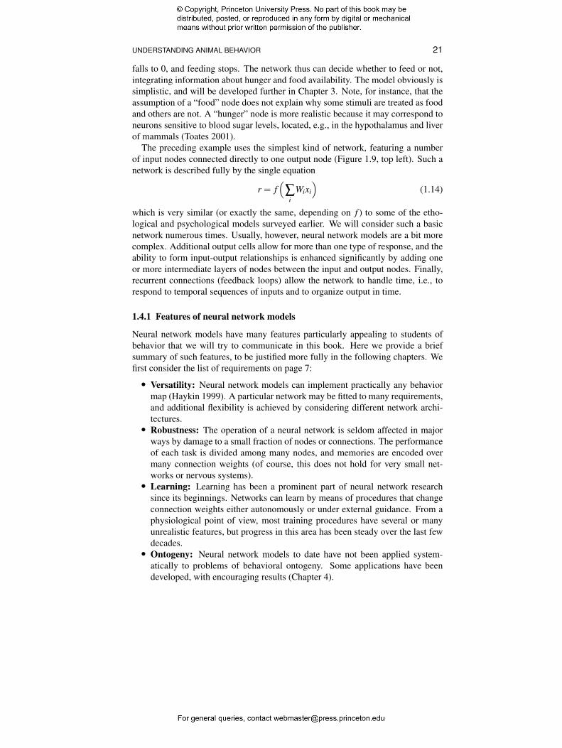
19 UNDERSTANDING ANIMAL BEHAVIOR

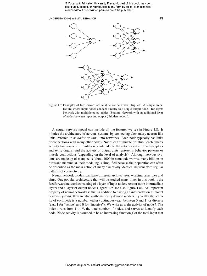
Figure 1.9 Examples of feedforward artificial neural networks. Top left: A simple archi­tecture where input nodes connect directly to a single output node. Top right: Network with multiple output nodes. Bottom: Network with an additional layer of nodes between input and output (“hidden nodes”).

A neural network model can include all the features we see in Figure 1.8. It mimics the architecture of nervous systems by connecting elementary neuron­like units, referred to as nodes or units, into networks. Each node typically has links or connections with many other nodes. Nodes can stimulate or inhibit each other’s activity like neurons. Stimulation is entered into the network via artificial receptors and sense organs, and the activity of output units represents behavior patterns or muscle contractions (depending on the level of analysis). Although nervous sys­tems are made up of many cells (about 1000 in nematode worms, many billions in birds and mammals), their modeling is simplified because their operation can often be described as the mass action of many essentially identical neurons with regular patterns of connectivity.

Neural network models can have different architectures, working principles and aims. One popular architecture that will be studied many times in this book is the feedforward network consisting of a layer of input nodes, zero or more intermediate layers and a layer of output nodes (Figure 1.9, see also Figure 1.8). An important property of neural networks is that in addition to having an interpretation as model nervous systems, they are also mathematically defined models. Typically, the activ­ity of each node is a number, either continuous (e.g., between 0 and 1) or discrete (e.g., 1 for “active” and 0 for “inactive”). We write as zi the activity of node i. The index i runs from 1 to N, the total number of nodes, and serves to identify each node. Node activity is assumed to be an increasing function f of the total input that

20 CHAPTER 1

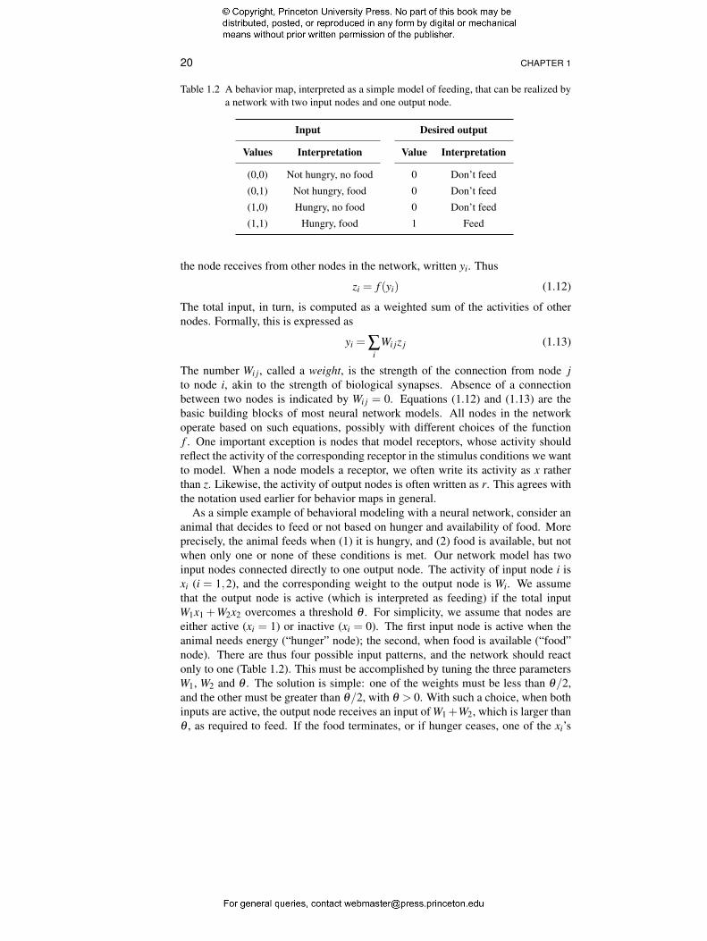
Table 1.2 A behavior map, interpreted as a simple model of feeding, that can be realized by a network with two input nodes and one output node.

Input Desired output

Values Interpretation Value Interpretation

(0,0) Not hungry, no food 0 Don’t feed

(0,1) Not hungry, food 0 Don’t feed

(1,0) Hungry, no food 0 Don’t feed

(1,1) Hungry, food 1 Feed

the node receives from other nodes in the network, written yi. Thus

zi = f (yi) (1.12)

The total input, in turn, is computed as a weighted sum of the activities of other nodes. Formally, this is expressed as

yi = ∑Wi jz j (1.13) i

The number Wi j, called a weight, is the strength of the connection from node j to node i, akin to the strength of biological synapses. Absence of a connection between two nodes is indicated by Wi j = 0. Equations (1.12) and (1.13) are the basic building blocks of most neural network models. All nodes in the network operate based on such equations, possibly with different choices of the function f . One important exception is nodes that model receptors, whose activity should reflect the activity of the corresponding receptor in the stimulus conditions we want to model. When a node models a receptor, we often write its activity as x rather than z. Likewise, the activity of output nodes is often written as r. This agrees with the notation used earlier for behavior maps in general.

As a simple example of behavioral modeling with a neural network, consider an animal that decides to feed or not based on hunger and availability of food. More precisely, the animal feeds when (1) it is hungry, and (2) food is available, but not when only one or none of these conditions is met. Our network model has two input nodes connected directly to one output node. The activity of input node i is xi (i = 1, 2), and the corresponding weight to the output node is Wi. We assume that the output node is active (which is interpreted as feeding) if the total input W1x1 + W2x2 overcomes a threshold θ . For simplicity, we assume that nodes are either active (xi = 1) or inactive (xi = 0). The first input node is active when the animal needs energy (“hunger” node); the second, when food is available (“food” node). There are thus four possible input patterns, and the network should react only to one (Table 1.2). This must be accomplished by tuning the three parameters W1, W2 and θ . The solution is simple: one of the weights must be less than θ/2, and the other must be greater than θ/2, with θ > 0. With such a choice, when both inputs are active, the output node receives an input of W1 +W2, which is larger than θ , as required to feed. If the food terminates, or if hunger ceases, one of the xi’s

21 UNDERSTANDING ANIMAL BEHAVIOR

falls to 0, and feeding stops. The network thus can decide whether to feed or not, integrating information about hunger and food availability. The model obviously is simplistic, and will be developed further in Chapter 3. Note, for instance, that the assumption of a “food” node does not explain why some stimuli are treated as food and others are not. A “hunger” node is more realistic because it may correspond to neurons sensitive to blood sugar levels, located, e.g., in the hypothalamus and liver of mammals (Toates 2001).

The preceding example uses the simplest kind of network, featuring a number of input nodes connected directly to one output node (Figure 1.9, top left). Such a network is described fully by the single equation

r = f � ∑Wixi

�(1.14)

i

which is very similar (or exactly the same, depending on f ) to some of the etho­logical and psychological models surveyed earlier. We will consider such a basic network numerous times. Usually, however, neural network models are a bit more complex. Additional output cells allow for more than one type of response, and the ability to form input­output relationships is enhanced significantly by adding one or more intermediate layers of nodes between the input and output nodes. Finally, recurrent connections (feedback loops) allow the network to handle time, i.e., to respond to temporal sequences of inputs and to organize output in time.

1.4.1 Features of neural network models

Neural network models have many features particularly appealing to students of behavior that we will try to communicate in this book. Here we provide a brief summary of such features, to be justified more fully in the following chapters. We first consider the list of requirements on page 7:

• Versatility: Neural network models can implement practically any behavior map (Haykin 1999). A particular network may be fitted to many requirements, and additional flexibility is achieved by considering different network archi­tectures.

• Robustness: The operation of a neural network is seldom affected in major ways by damage to a small fraction of nodes or connections. The performance of each task is divided among many nodes, and memories are encoded over many connection weights (of course, this does not hold for very small net­works or nervous systems).

• Learning: Learning has been a prominent part of neural network research since its beginnings. Networks can learn by means of procedures that change connection weights either autonomously or under external guidance. From a physiological point of view, most training procedures have several or many unrealistic features, but progress in this area has been steady over the last few decades.

• Ontogeny: Neural network models to date have not been applied system­atically to problems of behavioral ontogeny. Some applications have been developed, with encouraging results (Chapter 4).

22 CHAPTER 1

• Evolution: Various features of neural network models, such as architecture, learning rules and properties of connections and nodes, can be assumed to arise from different “genes.” Computer simulations of behavioral evolution can be set up to investigate what networks evolve to solve particular tasks. Such investigations are still at their beginnings. One obstacle is that we still ignore a lot about how genes control nervous system development.

Other features of neural network models are also relevant to modeling behavior:

• Structural constraints: The structure of these models essentially is based on knowledge of the nervous system: it is not inferred from observations of be­havior or from functional considerations. In this sense, neural network models are unique among models of behavior. Such constraints, when used properly, can greatly diminish the danger of introducing processes that cannot have a counterpart in biological nervous systems.

• Parallel processing: Processing in neural network is mainly parallel rather than sequential, as in digital computers. This means that the processes from reception of stimuli to responses can occur in much fewer cycles of operation, each consisting of many thousands or millions of simultaneous computations. This is an important step toward matching the abilities of nervous systems to react very quickly in a large range of conditions.

• Generalization: In new situations, animals show systematic generalization based on similar past conditions, and this is a crucial part of their ability to confront the world. As a consequence of their structure, many network models generalize naturally. This is a great advantage compared with models that either ignore generalization (Section 1.3.2) or simply assume that it occurs (Section 3.3.3).

• Definiteness and accessibility: Since neural network models are specified formally, they can be investigated in all details of operation. They can be stud­ied with tools such as the theory of dynamical systems and computer simula­tions or in much the same ways as neurophysiologists study nervous systems. For instance, one can study what happens when a specific part of the network is damaged or removed. This can bring insight into network operation and can also be compared with lesion studies in nervous systems.

• Unifying power: Neural network models can be applied to all aspects of be­havior: processing of stimuli, central processing and motor control. Neural networks can learn, and the substrate of memory (connection weights) is clear. Most approaches to behavior, on the other hand, are geared toward specific as­pects (e.g., perception or cognition) and may have problems at producing a unified theory of behavior.

1.4.2 A brief history

The history of neural network models is rooted in attempts to understand the ner­vous system and behavior, starting with the discovery by Santiago Ramòn y Cajal, Camillo Golgi and others at the end of the 19th century that the nervous system is composed of an intricate network of cells. Developments of neural network mod­

23 UNDERSTANDING ANIMAL BEHAVIOR

Figure 1.10 Rosenblatt’s (1958; 1962) perceptron, as depicted by Minsky & Papert (1969). Each ϕ is assumed to be 0 or 1 depending on the result of a simple computa­tion based on the state of a limited number of receptors. The summation unit Ω performs a weighted sum of the ϕ’s. If the sum is larger than a threshold value, the perceptron response Ψ is 1; if the sum is smaller than the threshold, the response is 0. Reprinted by permission from Minsky and Papert (1969). Perceptrons. The MIT Press.

els, however, are also rooted in mathematics, theories for intelligent machines and philosophy (Crevier 1993; Minsky 1969; Wang 1995).

The development of neural network models started in earnest in 1943 when War­ren McCulloch and Walter Pitts described how arbitrary logical operations could be carried out by networks of nodes (so­called formal neurons) that could either respond or not respond to an input, computed as the weighted sum of the activation state of other nodes in the network (McCulloch & Pitts 1943). This way of comput­ing the total input to a node has stayed in practically all later neural network models. An important aspect of McCulloch and Pitts’ work was that neural processing could be formulated mathematically. Six years later, Donald Hebb published his famous book, The Organization of Behavior, which, among other things, includes a theory of how connection strengths between nerve cells may act as memory and how such memory may change as a consequences of experiences (Hebb 1949). Perhaps the first full­blown neural network model was designed and simulated on computers by Frank Rosenblatt (1958, 1962). His “perceptron” is depicted in Figure 1.10. An important aspect of Rosenblatt’s work was providing the perceptron with a learning algorithm that allowed it to solve a wide range of classification problems, whereby each of many input patterns should be assigned to one of two categories. Bernard Widrow and Marcian Hoff further developed learning algorithms introducing a gen­eral procedure for training two­layer networks (Widrow & Hoff 1960), to be known later as the δ rule (Section 2.3.2).

The early enthusiasm for neural network models was subdued in 1969 by Min­sky and Papert’s book, Perceptrons, pointing out some severe limitations of per­ceptrons. Perceptrons cannot solve all categorization problems, and some that are solvable in principle are very hard to solve in practice (Chapter 2). The authors also suggested that multilayer networks would suffer from similar limitations, but

24 CHAPTER 1

this turned out to be incorrect. Minsky and Papert also acknowledged that recurrent networks (with feedback loops) could be much more capable (Chapters 2 and 3) but did not discuss them for several reasons. One was a desire to compare parallel com­puters (i.e., neural networks) with traditional serial computers; recurrent networks have both serial and parallel elements and thus were set aside. The perceptron was also chosen for its relative mathematical simplicity, which made a comprehensive analysis feasible. The book is nevertheless very interesting and contains many in­sights about neural networks that may also apply to biological nervous systems.

The 1980s saw a series of important publications that inspired a new wave of research into neural network theory and applications. Efficient learning algorithms for multilayer networks were made widely known, such as the now­celebrated back­propagation algorithm, and it was shown that multilayer feedforward net­works could overcome some limitations of perceptrons (Ackley et al. 1985; Haykin 1999; Rumelhart et al. 1986). Recurrent networks were also studied, and it was de­scribed how information could be stored in recurrent networks (Amit 1989; Cohen & Grossberg 1983; Hopfield 1982). Kohonen (1982) also published his results on self­organizing maps, showing how simple learning rules could organize networks based on experience without external guidance. Crucial to the diffusion of neural networks into cognitive psychology was the two­volume book, Parallel Distributed Processing: Explorations in the Microstructures of Cognition edited by James Mc­Clelland and David Rumelhart (1986; Rumelhart & McClelland 1986b).

To date, the study of artificial neural network has generated an extensive body of theory (e.g., Arbib 2003; Haykin 1999). Neural networks have proved to be a powerful explanatory tool applied to a wide variety of phenomena such as per­ception, concept learning, the development of motor skills, language acquisition in humans and studies of amnesia and brain damage (Arbib 2003; Churchland 1995; Churchland & Sejnowski 1992; McClelland & Rumelhart 1986). Recent progress has occurred along several lines. One is the study of more powerful and/or bio­logically realistic network architectures, e.g., recurrent networks that can handle time (Elman 1990; Jordan 1986). Fundamental areas of research are how networks can be trained to solve a specific task and how they can learn from experiences without explicit supervision. From the present perspective, an important issue is the development of more biologically realistic learning mechanisms. Many meth­ods for training networks are not realistic because they are external to the network rather than built into the network itself, but significant improvements have been achieved (Chapters 2 and 4). This is one area that needs more research, and it is important to recognize that besides all the progress, a number of issues remain to be resolved. Other areas in need of further research are, for instance, the genetic control of network development and how unrealistic retroactive interference (new learning destroying earlier memories) can be tackled (French 1999).

The preceding sketch of the history of neural network models is, of course, far from complete. The development of neural network models, for instance, has also benefited from the gains in our understanding of neurophysiology. Examples are the discovery of receptive fields in visual perception (Hubel & Wiesel 1962) and the study of learning in invertebrates (Kandel et al. 2000; Morris et al. 1988). There are also engineering applications that are of potentially great interest to biology and be­

25 UNDERSTANDING ANIMAL BEHAVIOR

havior, such as research into robotics (McFarland & Bösser 1993; Nolfi & Floreano 2000; Webb 2001). Designing functional robots based on neural networks forces the engineer to think about design issues similar to the ones evolution has tackled in animals. This is often revealing for biologists because it highlights problems of design that otherwise may be ignored or considered trivial. For instance, biolo­gists and psychologists often step over the problem of recognizing stimuli based on retinal images. This is a far from trivial task that people working with robots are forced to consider. Readers who are interested in a more complete history of neural network models are referred to Arbib (2003) and Haykin (1999).

1.4.3 Neural network models in animal behavior research

It may seem obvious that students of animal behavior should have embraced neural network models, but this has not been the case. The situation is rather the op­posite. With some exceptions, neural network models have been ignored among ethologists, behavioral ecologists and animal psychologists. For instance, they are absent from most textbooks on animal behavior. The most important exception, of course, is neuroethologists (Cliff 2003; Simmons & Young 1999), but their focus is not primarily on general theories of behavior in the sense discussed in this chapter. Neural networks are now increasingly popular in neuroscience (e.g., Dayan & Ab­bott 2001), where recent and important advances on our understanding of learning rely extensively on neural network models (Chapter 4).

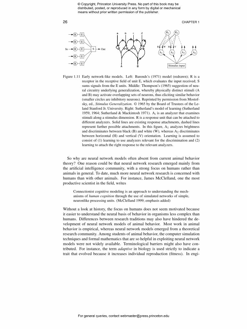
Of course, students of animal behavior have thought regularly about the neu­ral machinery underlying behavior. For example, both Ivan Pavlov and Edward Thorndike speculated on the nervous structures behind their behavioral observa­tions. The concept of connectionism, now often used as a label for neural network research, can also be traced back to these pioneers (Kandel et al. 2000; Mowrer & Klein 2001). Less often recognized are a number of network­like models by etholo­gists and animal psychologists (Baerends 1971; Blough 1975; Fentress 1976; Hinde 1970; Horn 1967; Sutherland 1959; Thompson 1965). Figure 1.11 shows three such models. Baerend’s (1971) model at top left is similar to Rosenblatt’s per­ceptron (Figure 1.10) and continues the tradition of ethological summation models (Section 1.3.3). The response arises from the weighted sum of signals from “eval­uation units” (E), which in turn analyze signals from receptors (R). The model by Blough (1975; discussed in Chapter 3) has a similar structure and also rediscovers Widrow and Hoff’s learning rule first published in 1960. Figure 1.11 also shows Thompson’s model from 1965. Its aim was to illustrate how generalization (sim­ilar responses to different stimuli) can arise from the fact that similar stimuli are processed by partially overlapping sets of neurons. This is a classical idea, present in Pavlov (1927), as well as in current neural network models (Chapter 3). The last model in the figure is Sutherland’s intriguing model from as early as 1959. It depicts a multilayer network with adjustable connections around the same time as Rosenblatt published his work on perceptrons (Sutherland 1959, 1964; Suther­land & Mackintosh 1971). It is interesting that these early efforts by biologist and psychologists developed with little or no contact with that part of the artificial in­telligence community that in the same years actively pursued neural networks.

26 CHAPTER 1

S

R E

R E

R E

R E

R E

In Out

Stimulus input

A1 A2 A3 A4

R1 R2

B W H V

Figure 1.11 Early network­like models. Left: Barends’s (1971) model (redrawn); R is a receptor in the receptive field of unit E, which evaluates the input received; S sums signals from the E units. Middle: Thompson’s (1965) suggestion of neu­ral circuitry underlying generalization, whereby physically distinct stimuli (A and B) may activate overlapping sets of neurons, thus eliciting similar behavior (smaller circles are inhibitory neurons). Reprinted by permission from Mostof­sky, ed., Stimulus Generalization. © 1965 by the Board of Trustees of the Le­land Stanford Jr. University. Right: Sutherland’s model of learning (Sutherland 1959, 1964; Sutherland & Mackintosh 1971). Ai is an analyzer that examines stimuli along a stimulus dimension. R is a response unit that can be attached to different analyzers. Solid lines are existing response attachments, dashed lines represent further possible attachments. In this figure, A1 analyzes brightness and discriminates between black (B) and white (W), whereas A2 discriminates between horizontal (H) and vertical (V) orientation. Learning is assumed to consist of (1) learning to use analyzers relevant for the discrimination and (2) learning to attach the right response to the relevant analyzers.

So why are neural network models often absent from current animal behavior theory? One reason could be that neural network research emerged mainly from the artificial intelligence community, with a strong focus on humans rather than animals in general. To date, much more neural network research is concerned with humans than with other animals. For instance, James McClelland, one the most productive scientist in the field, writes

Connectionist cognitive modeling is an approach to understanding the mech­anisms of human cognition through the use of simulated networks of simple, neuronlike processing units. (McClelland 1999; emphasis added)

Without a look at history, the focus on humans does not seem motivated because it easier to understand the neural basis of behavior in organisms less complex than humans. Differences between research traditions may also have hindered the de­velopment of neural network models of animal behavior. Most work in animal behavior is empirical, whereas neural network models emerged from a theoretical research community. Among students of animal behavior, the computer simulation techniques and formal mathematics that are so helpful in exploiting neural network models were not widely available. Terminological barriers might also have con­tributed. For instance, the term adaptive in biology is used strictly to indicate a trait that evolved because it increases individual reproduction (fitness). In engi­

27 UNDERSTANDING ANIMAL BEHAVIOR

neering and cognitive science the expression adaptive system has a broader scope and refers to any system that can change to better serve its purpose. Engineers thus may speak of adaptation when biologists would speak of learning. Another example is neural network theory referring to self­organization where ethologists would talk of learning or development and experimental psychologists of percep­tual learning. Important terms such as reinforcement and association are also used in slightly different ways.

In conclusion, traditional ethological and animal psychological thinking contains a number of seeds to neural network models, but the development of neural network theory has occurred mainly outside these disciplines. Neural network models still have not gained broad popularity in animal behavior research, but there is today a growing interest in neural networks, particularly among animal psychologists.

1.4.4 The diversity of network models: Our approach

To apply neural networks to animal behavior, we need to decide which particular models to use. This is not always easy. Neural network models come in many forms and purposes. There are biologically or psychologically motivated models with aims ranging from the very details of neural mechanisms to the highest mental functions in humans. There are models aimed primarily at machine intelligence and engineering applications with little concern for biological realism. The latter never­theless can be of interest to modeling animal behavior for practical and theoretical reasons. In this book we try to use simple networks as long as they can account for the behavior we investigate. There are a number of reasons for this approach. First, complexity should not be introduced prematurely and without reason. We could try to include from the start all known details of nervous systems, but this would result in a model as difficult to understand as the real system. The only way to understand a complex structure is to start by abstracting pieces from it or study simplified models that are more readily analyzed. The crucial test of a simplified model is the extent to which it captures essential features of the behavior of real an­imals. If it does, then the fact that the model is neurally inspired rather than based on some other metaphor should be considered a bonus rather than a hindrance.

Second, we need models of animal behavior that are easy to understand and prac­tical to use. We also need for general models as opposed to specific to a particular behavior and a particular species. The subject of animal behavior covers species with a nervous system made up of a few cells to the complexity of primate brains, and we know that many behavioral phenomena are surprisingly general.

Third, the differences between network models should not be exaggerated. Start­ing from a simple model such as Rosenblatt’s perceptron, we can add complexity gradually and in several ways. For instance, we can add more layers of nodes, recurrent connections and more complex node dynamics. We thus can obtain com­plex models gradually from simple ones and study how their properties change in the process. This is also relevant when studying the evolution from simple to complex behavior (Chapter 5).

In practice, our approach means that multilayer feedforward networks operating in discrete time are our first choice of model. Indeed, most applications of neu­

28 CHAPTER 1

ral networks are of this kind. If such models prove insufficient to analyze a given behavioral finding, we consider additional elements such as recurrent connections or dynamics in continuous time. Note that we do not deny the importance of de­tailed models. If neural network models are to fulfill their promises, the future will contain simple, intuitive, general and practical models, as well as detailed models closer to real nervous systems.

CHAPTER SUMMARY

• “Behavior” is a legitimate level of analysis. It has theoretical importance in ethology, psychology, behavioral ecology and evolutionary biology and prac­tical importance to many people working and living with animals in zoos, veterinary clinics, farms, etc.

• Explaining behavior includes understanding how motivational factors control responding, how behavior develops during an individual’s lifetime and how evolution shapes behavior. Understanding of actual internal processes may also be important.

• Most attempts to understand animal behavior have inferred models from be­havioral observations and functional considerations. This is true for most of ethology, experimental psychology and cognitive psychology. A major excep­tion is neuroethology, which studies how nervous systems generate behavior.

• Neural network models offer a potential to develop models of behavior that are informed not only by behavioral observations but also by the actual structure of nervous systems. Can this result in increased knowledge about behavior? Our aim is to explore this question. We have also touched on some fundamental issues about how to model behav­• ior, from neurophysiology to “cognition.” On important issue is how to deal with animals’ internal states. We will return to these issues throughout this book and in the concluding chapter.

FURTHER READING

Ethological and biological theory of behavior:

Eibl­Eibesfeldt I, 1975. Ethology: The Biology of Behavior. New York: Holt, Rinehart & Winston.

Hinde RA, 1970. Animal Behaviour. Tokyo: McGraw­Hill Kogakusha, 2 edition. Krebs JR, Davies NB, 1987. An Introduction to Behavioural Ecology. London:

Blackwell, 2 edition. McFarland DJ, 1999. Animal Behaviour: Psychobiology, Ethology and Evolu­

tion. Harlow, England: Longman, 3 edition.

Neuroethology:

Ewert JP, 1985. Concepts in vertebrate neuroethology. Animal Behaviour 33, 1–29.

29 UNDERSTANDING ANIMAL BEHAVIOR

Simmons PJ, Young D, 1999. Nerve Cells and Animal Behaviour. Cambridge, England: Cambridge University Press, 2 edition.

Animal learning theory, animal cognition, human cognition:

Klein SB, 2002. Learning: Principles and Applications. New York: McGraw­Hill, 4 edition.

Mackintosh NJ, editor, 1994. Animal Learning and Cognition. New York: Aca­demic Press.

Pearce JM, 1997. Animal Learning and Cognition. Hove, East Sussex: Psychol­ogy Press, 2 edition.

Shanks DS, 1995. The Psychology of Associative Learning. Cambridge, En­gland: Cambridge University Press.

For the discussion between behaviorism and cognitive psychology:

Leahey TH, 2004. A History of Psychology. Englewood Cliffs, NJ: Prentice­Hall, 6 edition.

Staddon JER, 2001. The New Behaviorism: Mind, Mechanism and Society. Hove, East Sussex: Psychology Press.

Neural network models:

Arbib MA, 2003. The Handbook of Brain Theory and Neural Networks. Cam­bridge, MA: MIT Press, 2 edition.

Churchland PM, 1995. The Engine of Reason, the Seat of the Soul: A Philosoph­ical Journey into the Brain. Cambridge, MA: MIT Press.

Churchland PS, Sejnowski T, 1992. The Computational Brain. Cambridge, MA: MIT Press.

Dayan P, Abbott LF, 2001. Theoretical Neuroscience: Computational and Math­ematical Modeling of Neural Systems. Cambridge, MA: MIT Press.

Haykin S, 1999. Neural Networks: A Comprehensive Foundation. New York: Macmillan, 2 edition.