Embed Size (px)
Citation preview

Characterization of seasonal effects on
the specific capacity of rope-pump
wells in a fractured rock-aquifer in
Nicaragua
Essa L. Gross and John S. GierkeDepartment of Geological Eng. & Sciences
Michigan Technological University
Antoinette KomeSNV Nicaragua

Outline
Problem Statement
Research Objectives
Study Area
Methodology
Results
Conclusions

Problem Statement
• Practically no information exists on the productivity of rural wells in developing countries.
• Policy makers have no information to base decisions or to develop water management plans.
• The lack of technical and economic resources prevents the collection of performance and monitoring data.

Design and test a method to characterize
the productivity of existing rope-pump
wells in rural areas of developing countries
Research Objectives
Monitor seasonal changes in SWLs
and specific capacities of rope-pump
wells in an area that experiences
distinct rainy and dry seasons.

Outline
Problem Statement
Research Objectives
Study Area
Methodology
Results
Conclusions
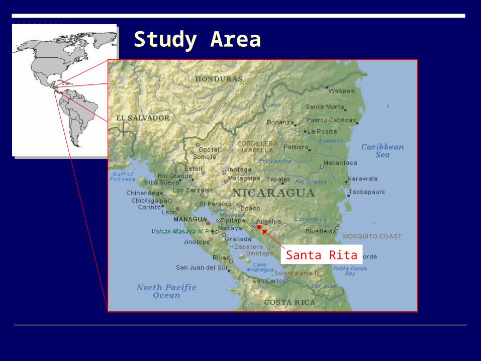
Santa Rita
Study Area
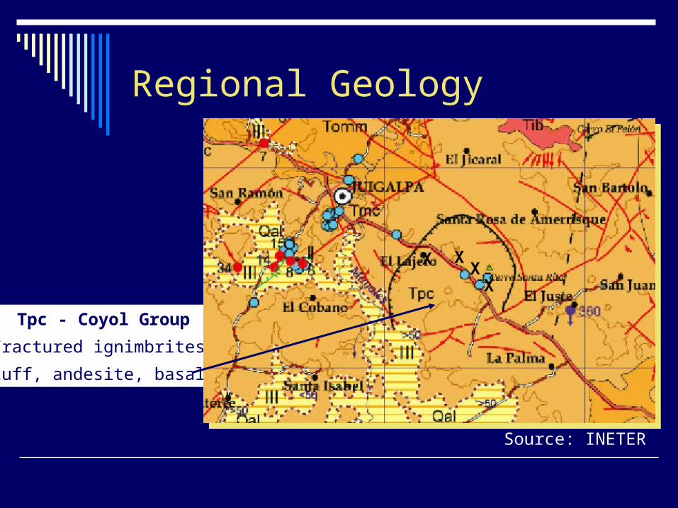
Regional Geology
Tpc - Coyol Group
Fractured ignimbrites,
tuff, andesite, basalt
X XX
X
Source: INETER
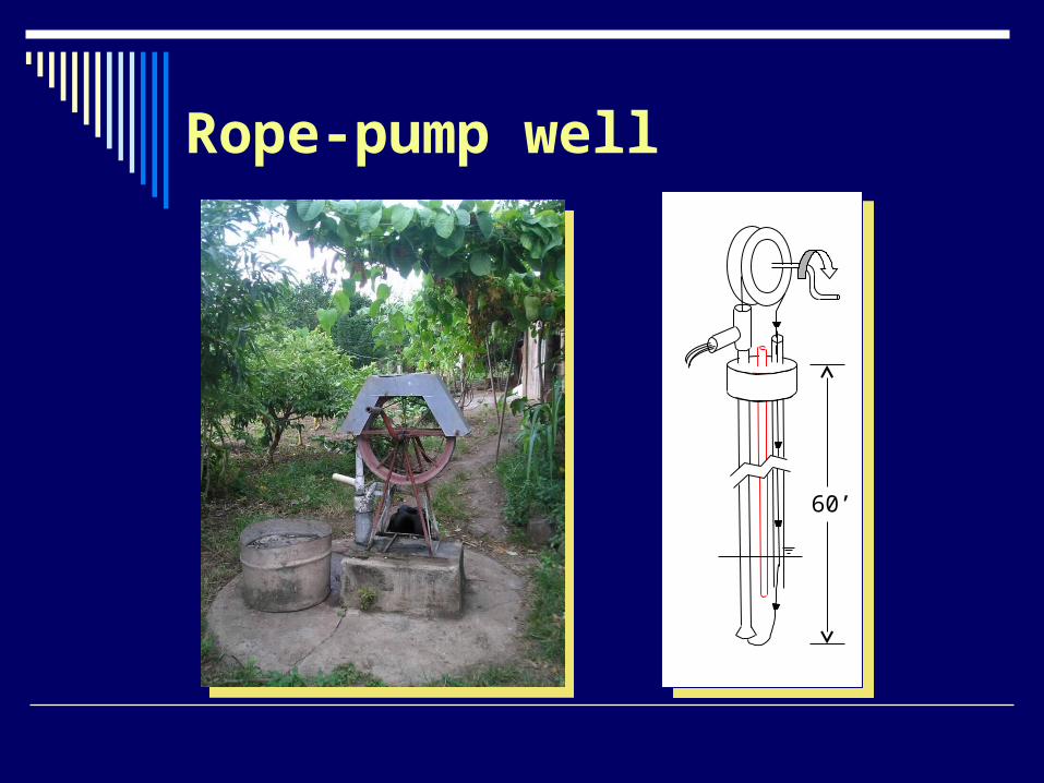
Rope-pump well
60’

Outline
Problem Statement
Research Objectives
Study Area
Methodology
Results
Conclusions
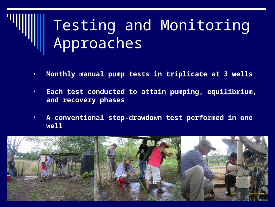
Testing and Monitoring Approaches
• Monthly manual pump tests in triplicate at 3 wells
• Each test conducted to attain pumping, equilibrium, and recovery phases
• A conventional step-drawdown test performed in one well
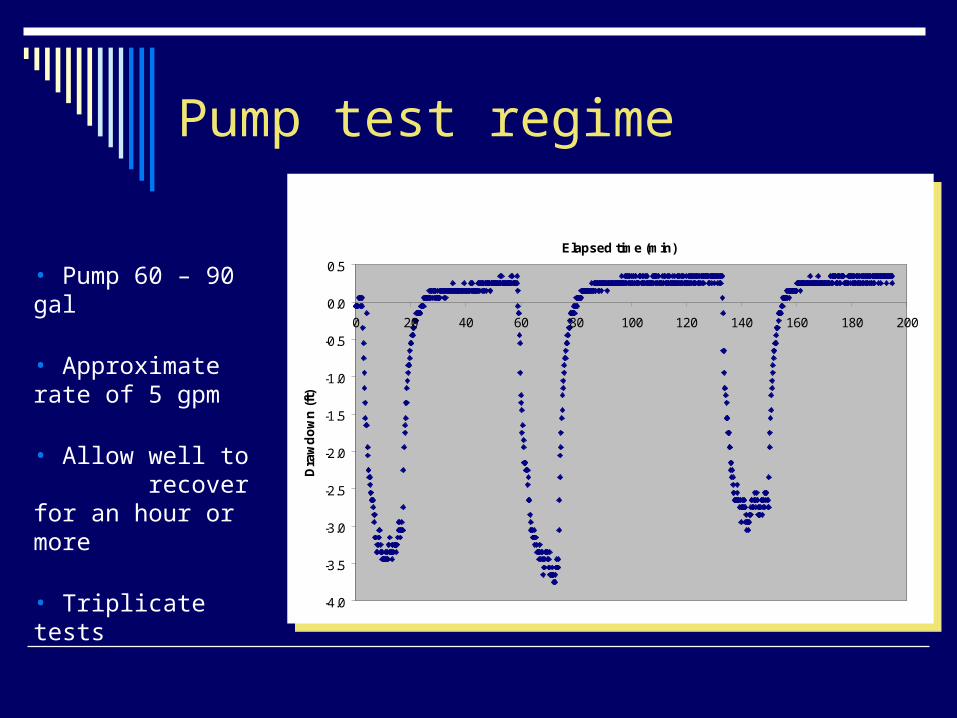
Pump test regime
• Pump 60 – 90 gal
• Approximate rate of 5 gpm
• Allow well to recover for an hour or more
• Triplicate tests
Well 2 - 2/10/07
-4.0
-3.5
-3.0
-2.5
-2.0
-1.5
-1.0
-0.5
0.0
0.5
0 20 40 60 80 100 120 140 160 180 200
Elapsed time (min)
Dra
wd
ow
n (
ft)
Well 2 - 2/10/07
-4.0
-3.5
-3.0
-2.5
-2.0
-1.5
-1.0
-0.5
0.0
0.5
0 20 40 60 80 100 120 140 160 180 200
Elapsed time (min)
Dra
wd
ow
n (
ft)
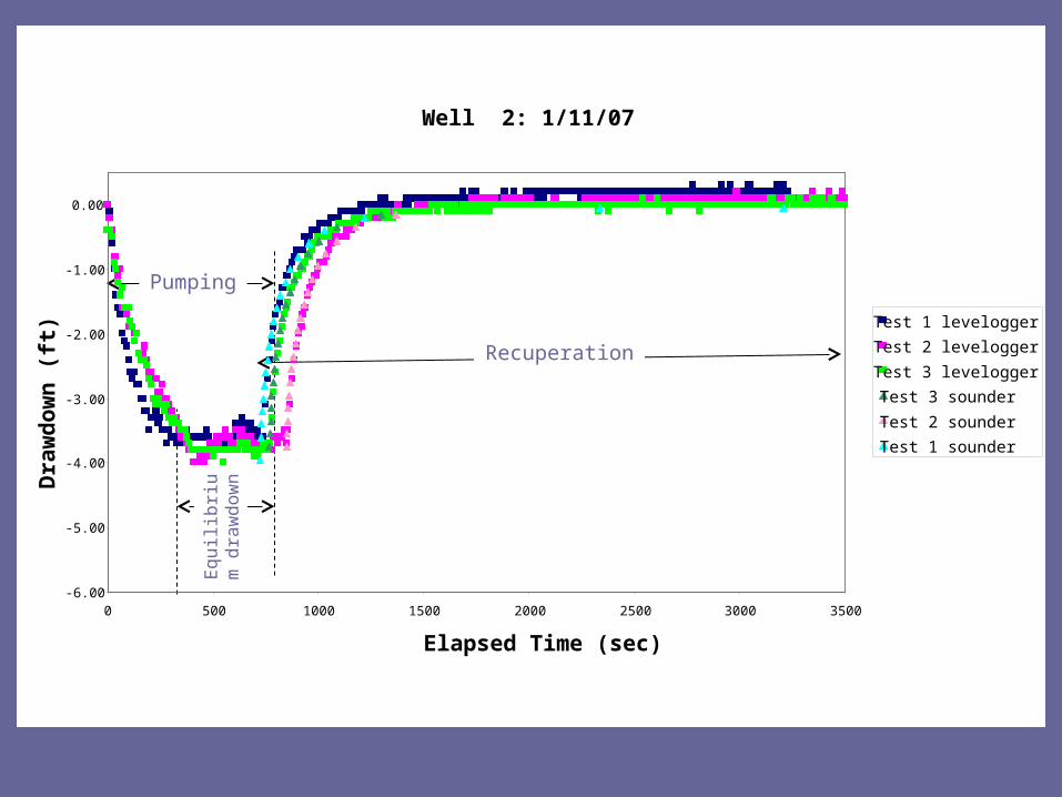
Recuperation
Eq
uili
briu
m
dra
wd
ow
n
Pumping
ExplanationWell 2: 1/11/07
-6.00
-5.00
-4.00
-3.00
-2.00
-1.00
0.00
0 500 1000 1500 2000 2500 3000 3500
Elapsed Time (sec)
Dra
wd
ow
n (
ft) Test 1 levelogger
Test 2 levelogger
Test 3 levelogger
Test 3 sounder
Test 2 sounder
Test 1 sounder
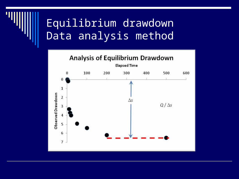
Equilibrium drawdown Data analysis method
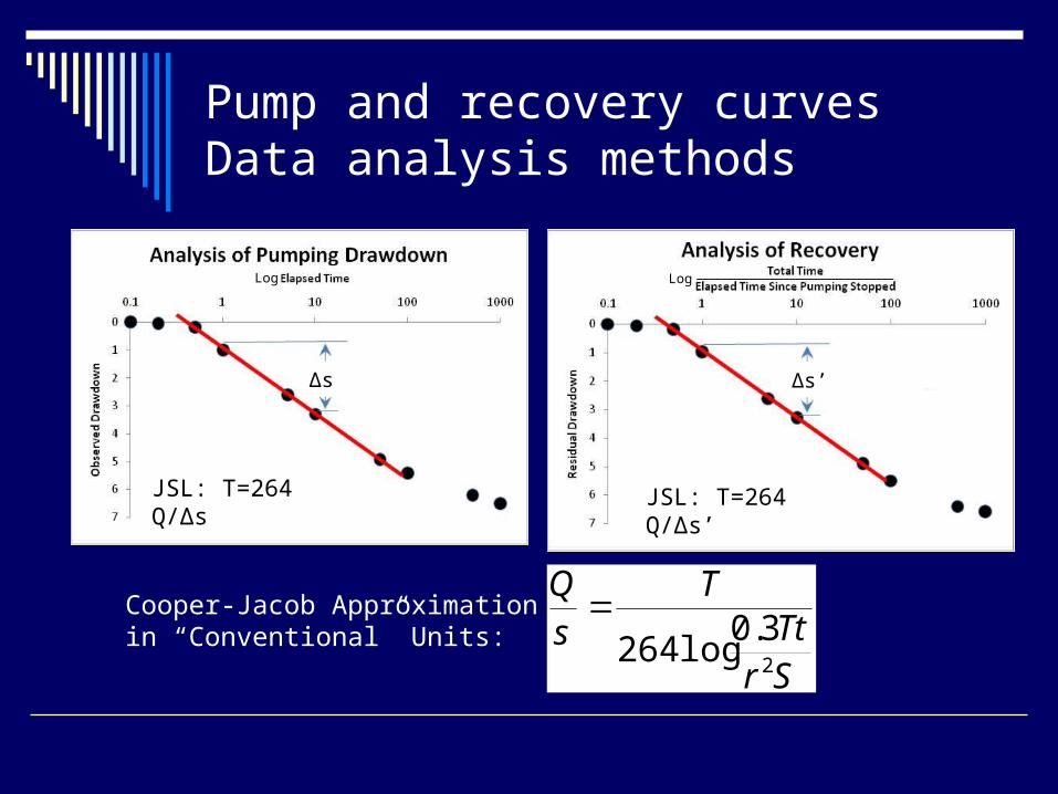
Pump and recovery curves Data analysis methods
SrTt
TsQ
2
3.0log264
Cooper-Jacob Approximation in “Conventional” Units:
Log Log
JSL: T=264 Q/Δs JSL: T=264 Q/Δs’
Δs Δs’

Outline
Problem Statement
Research Objectives
Study Area
Methodology
Results
Conclusions
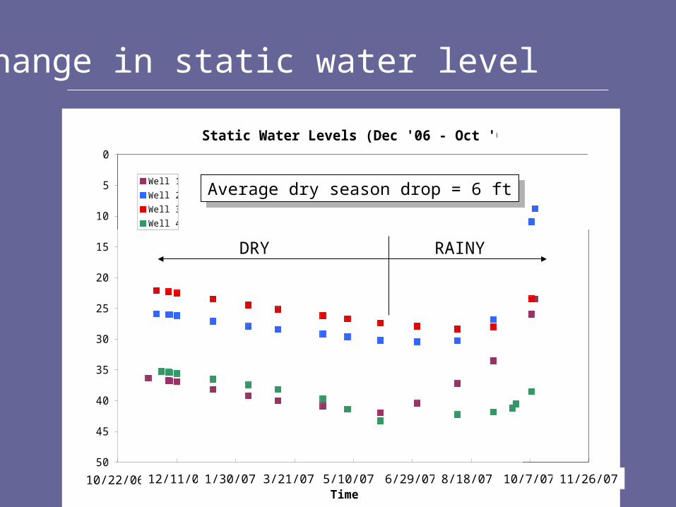
Change in static water level
Static Water Levels (Dec '06 - Oct '07)0
5
10
15
20
25
30
35
40
45
5010/22/06 12/11/06 1/30/07 3/21/07 5/10/07 6/29/07 8/18/07 10/7/07 11/26/07
Time
Sta
tic
Wate
r Level (
ft b
tc)
Well 1
Well 2
Well 3
Well 4
10/22/06 12/11/06 1/30/07 3/21/07 5/10/07 6/29/07 8/18/07 10/7/07 11/26/07
Average dry season drop = 6 ftAverage dry season drop = 6 ft
DRY RAINY
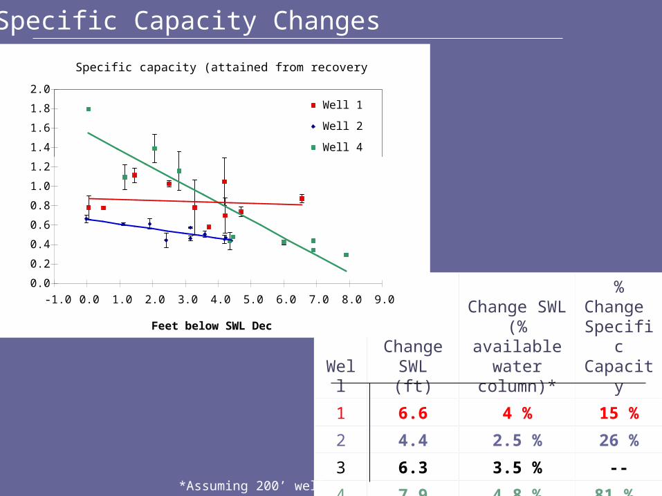
Specific Capacity Changes
WellChange SWL (ft)
Change SWL (% available
water column)*
% Change Specific Capacity
1 6.6 4 % 15 %
2 4.4 2.5 % 26 %
3 6.3 3.5 % --
4 7.9 4.8 % 81 % *Assuming 200’ well
0.0
0.2
0.4
0.6
0.8
1.0
1.2
1.4
1.6
1.8
2.0
-1.0 0.0 1.0 2.0 3.0 4.0 5.0 6.0 7.0 8.0 9.0
Feet below SWL Dec 06
Sp
ecif
ic c
apac
ity
(gp
m/f
t)
Well 1
Well 2
Well 4
Linear(Well 4)Linear(Well 2)Linear(Well 1)
Specific capacity (attained from recovery data) vs. SWL
Well 1
0.0
0.5
1.0
1.5
2.0
2.5
36.0 38.0 40.0 42.0 44.0Static Water level (ft btc)
Sp
ec
ific
Ca
pa
cit
y (
gp
m/f
t)
Non-equilibriumrecoverycurveEquilibriumapprox
Linear (Non-equilibriumrecoverycurve)
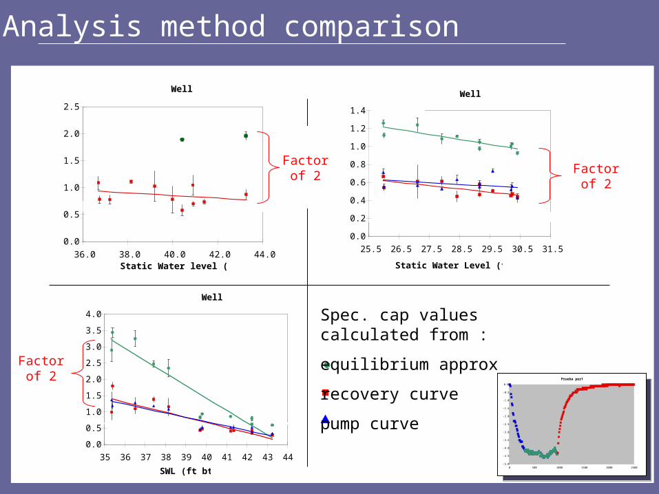
Analysis method comparison
Prueba perfil
-5.0
-4.5
-4.0
-3.5
-3.0
-2.5
-2.0
-1.5
-1.0
-0.5
0.0
0 500 1000 1500 2000 2500
Prueba perfil
-5.0
-4.5
-4.0
-3.5
-3.0
-2.5
-2.0
-1.5
-1.0
-0.5
0.0
0 500 1000 1500 2000 2500
Well 2
0.0
0.2
0.4
0.6
0.8
1.0
1.2
1.4
25.5 26.5 27.5 28.5 29.5 30.5 31.5
Static Water Level (ft btc)
Sp
ec
ific
ca
pa
cit
y (
gp
m/f
t)
Equilibriumapprox
Non-equilibriummethod -recoverycurveNon-equilibriummethod -pump curve
Linear(Equilibriumapprox)
Linear (Non-equilibriummethod -pump curve)
Linear (Non-equilibriummethod -recoverycurve)Well 4
0.0
0.5
1.0
1.5
2.0
2.5
3.0
3.5
4.0
35 36 37 38 39 40 41 42 43 44
SWL (ft btc)
Sp
ec
ific
ca
pa
cit
y (
gp
m/f
t)
Equilibriumapprox
Non-equilibriummethod -recovery curve
Non-equilibriummethod - pumpcurve
Linear (Non-equilibriummethod -recovery curve)Linear(Equilibriumapprox)
Linear (Non-equilibriummethod - pumpcurve)
Factorof 2
Factorof 2
Factorof 2
Spec. cap values calculated from :
equilibrium approx
recovery curve
pump curve
Well 4
0.0
0.5
1.0
1.5
2.0
2.5
3.0
3.5
4.0
35 36 37 38 39 40 41 42 43 44
SWL (ft btc)
Sp
ec
ific
ca
pa
cit
y (
gp
m/f
t)
Equilibriumapprox
Non-equilibriummethod -recovery curve
Non-equilibriummethod - pumpcurve
Trad Equilibriumapprox
Trad Non-equilibrium-pumpcurve
Trad Non-equilibrium-recovery curve
Linear (Non-equilibriummethod -recovery curve)Linear(Equilibriumapprox)
Linear (Non-equilibriummethod - pumpcurve)
Prueba perfil
-5.0
-4.5
-4.0
-3.5
-3.0
-2.5
-2.0
-1.5
-1.0
-0.5
0.0
0 500 1000 1500 2000 2500
Prueba perfil
-5.0
-4.5
-4.0
-3.5
-3.0
-2.5
-2.0
-1.5
-1.0
-0.5
0.0
0 500 1000 1500 2000 2500
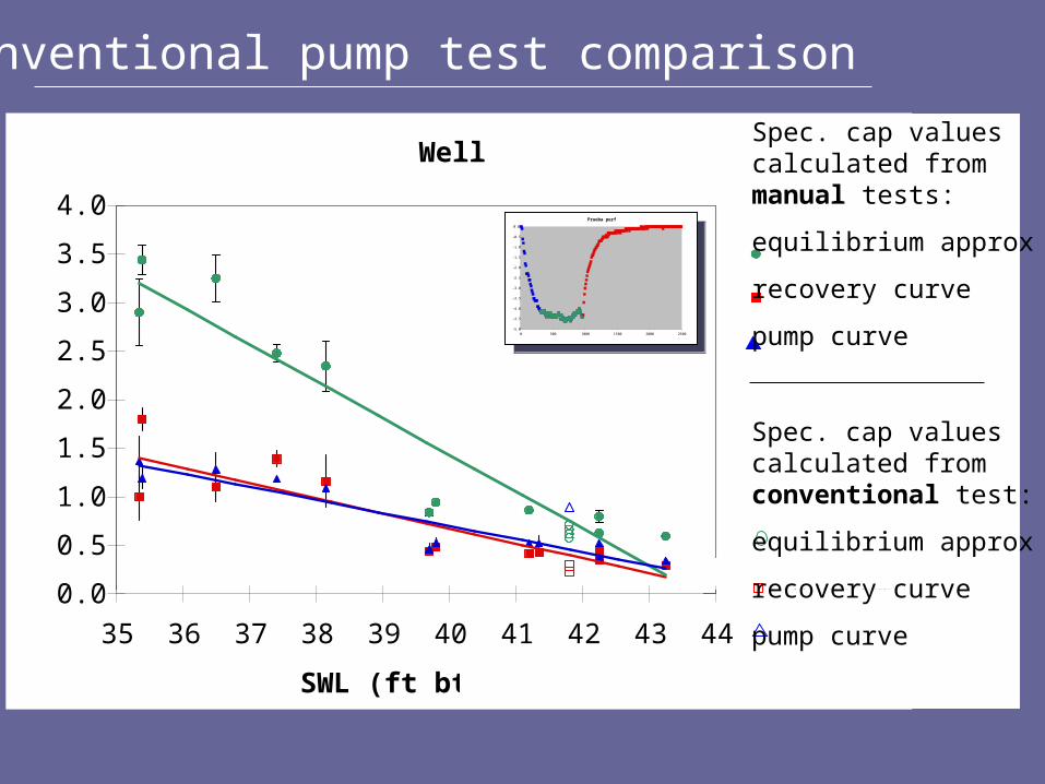
Spec. cap values calculated from manual tests:
equilibrium approx
recovery curve
pump curve
Spec. cap values calculated from conventional test:
equilibrium approx
recovery curve
pump curve
Conventional pump test comparison

Outline
Problem Statement
Research Objectives
Study Area
Methodology
Results
Conclusions
Conclusions (1 of 2)
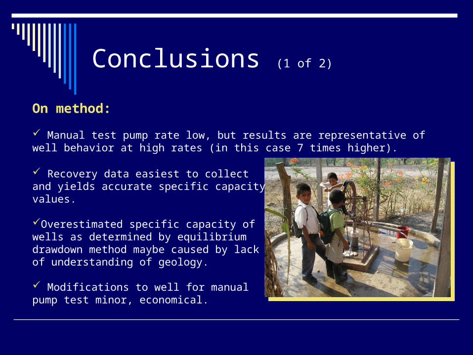
On method:
Manual test pump rate low, but results are representative of well behavior at high rates (in this case 7 times higher).
Recovery data easiest to collect and yields accurate specific capacity values.
Overestimated specific capacity of wells as determined by equilibrium drawdown method maybe caused by lack of understanding of geology.
Modifications to well for manual pump test minor, economical.
Conclusions (2 of 2)
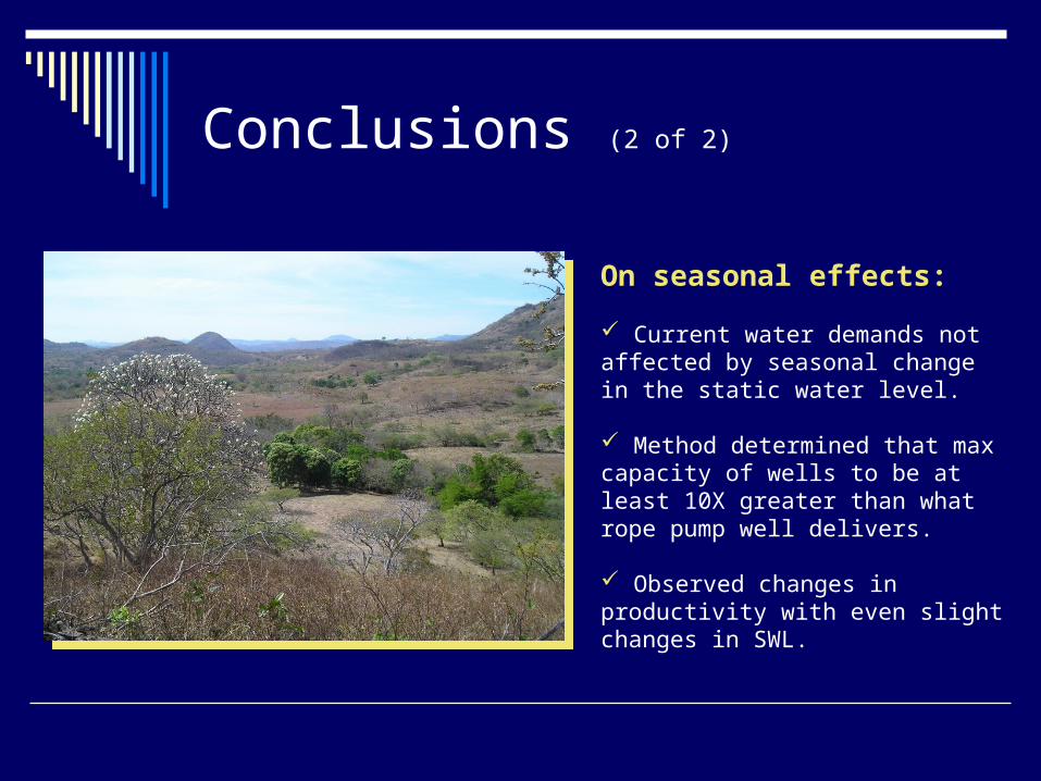
On seasonal effects:
Current water demands not affected by seasonal change in the static water level.
Method determined that max capacity of wells to be at least 10X greater than what rope pump well delivers.
Observed changes in productivity with even slight changes in SWL.

Thank You
We would like to acknowledge the following people for their assistance in this study:
Gregg Bluth, Fernando Flores, Luis Meza, Denia Acuña, Evelio Lopez , Ivan Palacios, Elisena Medrano, Luis Palacios, Beth Myre,
and the Families of Santa Rita
Financial Support:• National Science Foundation PIRE 0530109• DeVlieg Foundation• SNV Nicaragua• U.S. Peace Corps