Project-Driven Supply Chains: Integrating Inventory Planning

with Project Management ∗

Ching-Yu Chen

Department of International Business, Tunghai University, Taiwan

amychen@thu.edu.tw

Yao Zhao

Department of Supply Chain Management and Marketing Science

Rutgers University, Newark, NJ 07102

yaozhao@andromeda.rutgers.edu

First version July 2007, revised January and May 2008, March 2009

Abstract

We consider the strategic planning of recurrent projects and their material supplies over an

extended period of time. We propose a mathematic modeling framework – the project-driven

supply chain (PDSC) – to integrate project management (resource planning and scheduling

within each project) with material supply management (lead-time planning based on multi-

project statistics). For tree structure networks, we develop an optimization algorithm based

on dynamic programming. Using examples, we demonstrate that the PDSC model can lead to

significant cost savings as compared to the common practice which optimizes material supply

and project decisions separately. We develop insights on how the savings are generated and when

they are significant. We also discuss extensions of the model to include material customization,

non-consumable resource constraints and acyclic networks.

Keywords: Project-driven supply chain, project management, supply chain management, con-

sumable material, inventory positioning.∗Research supported by the grant no. 0747779 from the National Science Foundation.

1

1 Introduction

In this paper, we identify an important class of practical problems in which the supply chain

decisions and project decisions are intertwined. Our objective is to develop a modeling framework

to integrate these decisions and to demonstrate its potential by a comparison to the common

practice.

1.1 Motivation

It is not rare to find industries where projects are recurrent (subject to customization) and each

requires significant amount of modularized and standardized parts that are made elsewhere. Ex-

amples include construction, oil/gas well drilling industries.

Construction. An important trend in the construction industry is the so-called manufactured

housing (MH), also known as prefabricated housing or construction industrialization. The basic

principle of MH is to make housing components in factories (off-site), then assemble them on-

site. Traditional house construction incurs nearly 100% cost on site. With MH, off-site cost often

accounts for more than 50%. Off-site prefabricated housing components can be part of a house (e.g.,

exterior wall, stairs, balcony, kitchen/restroom) or even an entire house1. In 2003, MH represents

approximately 20 percent of the total housing market (Hastak and Syal 2004).

An important enabler for MH is the industry-wide modularization and standardization of com-

ponents and subsystems. Often coming along with MH is the reduced variety of floor plans (pre-

determined). By Kerwin (2005), Pulte Homes Inc. (the largest US homebuilder in 2009) offers

only the most popular floor plans (a reduction from 2200 to 600). In terms of procurement, Pulte

leverages its size to buy directly from suppliers (not through subcontractors), and distribute by its

own logistics network.

MH has changed the construction industry significantly. On one hand, MH leads to higher

quality, shorter project duration and much less labor cost and energy consumption. For instance,

Vanke (the largest residential developer in China), was able to cut project duration by 20%, water

consumption by 36% and electricity by 31% by increasing manufactured housing components from

nearly 0% to 37%2. On the other hand, MH poses significant challenges in both technology and1http://en.wikipedia.org/wiki/Manufactured housing2http://sz.house.sina.com.cn/news/2008-12-20/210926636.html

2

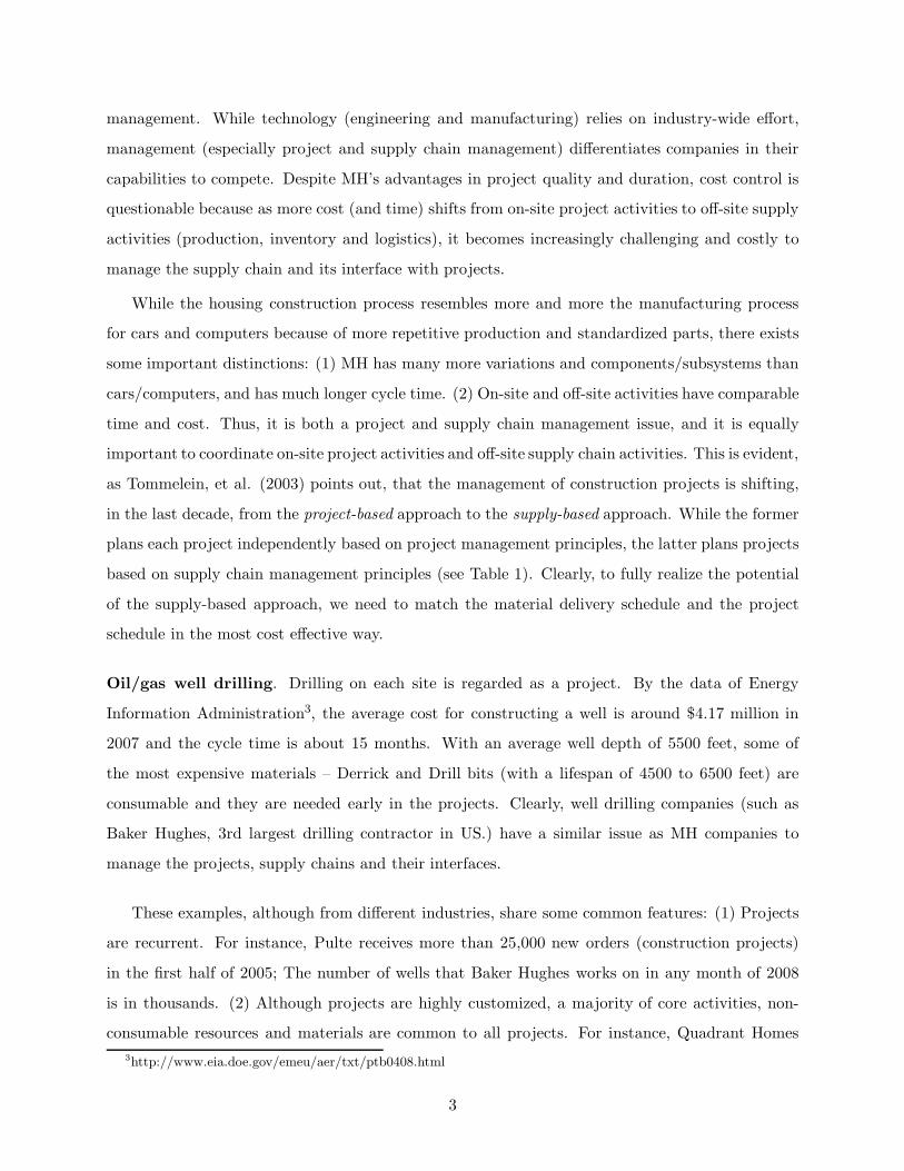
management. While technology (engineering and manufacturing) relies on industry-wide effort,

management (especially project and supply chain management) differentiates companies in their

capabilities to compete. Despite MH’s advantages in project quality and duration, cost control is

questionable because as more cost (and time) shifts from on-site project activities to off-site supply

activities (production, inventory and logistics), it becomes increasingly challenging and costly to

manage the supply chain and its interface with projects.

While the housing construction process resembles more and more the manufacturing process

for cars and computers because of more repetitive production and standardized parts, there exists

some important distinctions: (1) MH has many more variations and components/subsystems than

cars/computers, and has much longer cycle time. (2) On-site and off-site activities have comparable

time and cost. Thus, it is both a project and supply chain management issue, and it is equally

important to coordinate on-site project activities and off-site supply chain activities. This is evident,

as Tommelein, et al. (2003) points out, that the management of construction projects is shifting,

in the last decade, from the project-based approach to the supply-based approach. While the former

plans each project independently based on project management principles, the latter plans projects

based on supply chain management principles (see Table 1). Clearly, to fully realize the potential

of the supply-based approach, we need to match the material delivery schedule and the project

schedule in the most cost effective way.

Oil/gas well drilling. Drilling on each site is regarded as a project. By the data of Energy

Information Administration3, the average cost for constructing a well is around $4.17 million in

2007 and the cycle time is about 15 months. With an average well depth of 5500 feet, some of

the most expensive materials – Derrick and Drill bits (with a lifespan of 4500 to 6500 feet) are

consumable and they are needed early in the projects. Clearly, well drilling companies (such as

Baker Hughes, 3rd largest drilling contractor in US.) have a similar issue as MH companies to

manage the projects, supply chains and their interfaces.

These examples, although from different industries, share some common features: (1) Projects

are recurrent. For instance, Pulte receives more than 25,000 new orders (construction projects)

in the first half of 2005; The number of wells that Baker Hughes works on in any month of 2008

is in thousands. (2) Although projects are highly customized, a majority of core activities, non-

consumable resources and materials are common to all projects. For instance, Quadrant Homes3http://www.eia.doe.gov/emeu/aer/txt/ptb0408.html

3

Project-based Approach Supply-based Approach

Uniquely Engineered Facilities Assembly of Unique Facilities

and Components from Standardized Modules and Components

Competitive Bidding Emphasis on Long-term Working Relationships

Information Hoarding Create Information Visibility so that

the Value Chain Supports the Supply Chain

Liquidated Damages Problem Solving through Strategic Alliances

for Key Products and Components

Long and Uncertain Lead Times Short and Reliable Cycle Times

with Extensive Use of Expediting from Raw Materials to Site Installation

Early Delivery of All Phased Delivery of Materials to

Materials to the Site the Site to Match Installation Rates

Table 1: Project-based approach vs. supply-based approach.

Inc. follows a standard procedure in construction of residential housing with a fixed duration,

see Brown, et al. (2004). (3) Time and cost spent in project activities are comparable to those in

supply chain activities. We call problems with these features project-driven supply chains (PDSCs).

Clearly, these common features apply beyond the aforementioned industries, to some engineer-

procure-construct (EPC) projects where supply chain management poses a significant challenge in

managing the projects (Yeo and Ning 2002).

One of the major issues in PDSCs is the coordination between material delivery schedule with

project schedule. The trade-off here is between project cost and supply chain cost. Intuitively, the

shorter the supply chain lead times, the higher the supply chain cost, but more flexibility and lower

cost for project activities. On the contrary, the longer the supply chain lead times, the lower the

supply chain cost, but less flexibility and higher cost for project activities.

PDSCs require a new modeling paradigm to integrate supply chain and project management.

For this purpose, we present a modeling framework to capture the common features of a PDSC

and to optimally balance the trade-off by strategically planning for supply chains (off-site) lead

times and project resource (on-site). Mathematically, an PDSC model refers to a combination of

material supply chains where inventory can be held and a set of common activities and resources

constraints that define the projects, see Figure 1. Projects are recurrent and their occurrence

4

Figure 1: A project-driven supply chain (PDSC).

cannot be fully predicted in advance. Our objective is to jointly optimize project decisions (e.g.

scheduling, resource planning and allocation) within each project and supply chain decisions (lead

times) based on demand statistics across multiple projects, in order to coordinate material delivery

schedule with project schedule in the most cost effective way.

1.2 Summary of Results

In §3), we consider the basic PDSC model where all projects share the same set of activities and

materials. For simplicity, we drop the non-consumable resource constraints. Demand for materials

is determined by a forecast of future projects and statistics of current and past projects. The

material network interacts with the project network in the following ways: (1) The demand for the

material supply chains is generated by the material requirements of the projects. (2) The material

availability constrains the starting times of the project activities. Clearly, material lead times and

activity durations are competing for the due date. To optimally balance the inventory holding

costs and the activity direct cost/project delay penalties, we present a joint optimization model to

determine the optimal material lead time, activity durations and project schedule simultaneously

so as to minimize system-wide cost per unit of time.

In §4, we develop an optimization algorithm based on dynamic programming (DP) for tree

structure PDSCs. The DP algorithm generalizes that of Graves and Willems (2000, 2003a) from

a pure material supply chain to an PDSC. The complexity of the algorithm is polynomial in

5

the maximum service time and the maximum latest finishing time. Given the solution of the DP

algorithm, i.e., the committed service times from the supply network, one can determine the critical

path and slacks for the project network by the critical path method (CPM, see Nahmias 2005) with

additional material availability constraints on activity starting times.

Using simple examples (§5), we provide insight on when the joint optimization results in signif-

icant savings as compared to the common practice that makes supply chain and project decisions

sequentially. Even if the activity durations are fixed, coordinating the project schedule with inven-

tory decisions alone can result in sizable savings.

In §6, we extend the basic model to include material customization where material requirement

may vary across projects. We also discuss, in §7, extensions to include non-consumable resource

constraints, activity customization, acyclic PDSCs and economies of scale in material ordering.

2 Literature Review

The integration of supply chain and project management in general, and the PDSC modeling frame-

work in particular, is related to the literature of the following areas: Supply chain management,

project management, project scheduling and material ordering (PSMO), and construction manage-

ment. We shall review related literature in each area and point out the contribution of the PDSC

model.

Related Literature in Supply Chain Management. There is an extensive literature of supply

chain inventory management, mainly grown out of applications in the manufacturing industry.

We refer to Zipkin (2000), Porteus (2002) and Axsater (2006) for comprehensive reviews. The

literature focuses on material supplies but rarely touch on joint project-management and supply

chain management decision making.

Clearly, given the statistics of project occurences and fixing their schedules, the material re-

quirements are known statistically. Then the problem of managing material supplies becomes a

well-studied supply chain management issue. For inventory placement/positioning models in gen-

eral structure supply chains, we refer to Axsater (2006), Graves and Willems (2003b) and Simchi-

Levi and Zhao (2007) for recent reviews. Graves and Willems (2005) presents a general model

to optimize stock decisions and supply chain configurations simultaneously for new product intro-

ductions. All of these works focus on the material supply chain without considering the project

6

network and their interactions.

A PDSC is similar, in the network topology, to assembly systems in the manufacturing industry,

also see Zipkin (2000, pg 324) Section 8.4 for an analog between an assembly system and a project.

As opposed to typical manufacturing systems, construction projects occur less frequently in demand

and have higher degree of customization (O’Brien, et al 2002). The main difference between a

PDSC and a typical manufacturing system (make-to-stock or assemble-to-order) is that in the

former, one needs to schedule activities and allocate resources within each project, i.e., the project

management issues prevail, while in the latter, such issue can be ignored. Thus, the PDSC model

can be regarded as an extension of the supply chain management literature to include project

management decisions, by integrating lead time planning (based on multi-project statistics) with

project management (coordinating project activities and resources within each project).

As pointed by Vrijhoef and de Ridder (2006), a system with recurrent construction projects is

similar to an make-to-order (MTO) manufacturing system where each project can be regarded as a

final product. MTO manufacturing systems, especially, mass-customization, are studied extensively

in the literature. We refer to Gunasekaran and Ngai (2004) for a review on build-to-order (BTO)

supply chain management and Stevenson, et al. (2005) for a review on MTO production planning

and control. One major issue in planning and operations of MTO systems is the coordination of

internal operations and the integration between them and those of inbound suppliers. Two streams

of mathematical models prevail: (1) Stochastic models, which focus on workload control in job

shops using concepts such as Kanban and Constant WIP based on queuing theory. (2) Deterministic

models, which focus on resolving capacity and fixed cost issues for a given number of orders using

mixed integer programs. In practice, the inbound supplying activities and internal production

schedule are often planned and controlled by MRP type of systems. To our best knowledge, there

is no similar work (as the PDSC model) in this literature on integrated planning of material lead

times and resource allocation for each order.

Related Literature in Project Management and PSMO. The project management litera-

ture includes classic results on critical path method (CPM), time-costing analysis (TCA), project

evaluation and review techniques (PERT) and resource constrained project scheduling (RCPS). We

refer to Ozdamar and Ulusoy (1995), Pinedo (2005) and Jozefowska and Weglarz (2006) for recent

surveys.

Most work on RCPS focuses on non-consumable and reusable resources such as machine and

7

labor. For consumable resources (e.g., materials), one standard approach is to assume fixed lead

times and then model material procurement processes as activities. However, when lead times are

decision variables, we cannot model a supply chain (where inventory can be held at each node) by

a project network due to different dynamics/constraints imposed by a supply chain and a project

network (see §3 for more details).

Another approach to incorporate consumable resources is the PSMO which jointly plans for

project schedule and material order quantities. This approach is based on the following observation:

A project may repetitively require the same material over time. Given the project schedule, the

timing and size of material requirement is determined, which serve as input to optimize material

orders so as to balance the fixed ordering cost and inventory holding cost. Clearly, the project

scheduling and material ordering decisions are coupled, and the question is how to jointly optimize

both for a project. Aquilano and Smith (1980) initiated this approach by considering joint CPM and

MRP planning with constant activity durations. Smith-Daniels and Aquilano (1984) and Smith-

Daniels and Smith-Daniels (1987) present various extensions. More recently, Dodin and Elimam

(2001) include varying activity duration, early reward/late penalty and quantity discount into the

model.

The PDSC model complements the PSMO model by allowing material lead times to be decision

variables. While the PSMO model focuses on the cycle stock issues (economies of scale) in material

management, and jointly optimizes project schedule and material order quantities, the PDSC model

focuses on the safety-stock issues (uncertainty in the occurrence of future projects and their material

requirements), and jointly optimizes project schedule and material lead times.

Finally, the time-cost analysis (TCA) is a well developed technique in project management (see

Nahmias 2005) for managing project direct cost and delay. However, it has yet been integrated

with material lead time optimization. More recently, there is a trend in the project management

research community to study multi-project coordination (Vrijhoef and de Ridder 2006, Abdullah

and Vickridge 1999). These efforts focus on planning for multiple known projects without material

lead time decisions. The PDSC modeling framework extends the project management literature to

include lead time planning for consumable materials.

Related Literature in Construction Management. Cox and Ireland (2002) reviews the history

and the current status of the capital projects and construction industry. They pointed out that

due to short-term planning, adversarial relationship and high fragmentation of the industry, low

8

efficiency, low quality and high cost prevail. Hastak and Syal (2004) summarizes the current state

of the art in the manufactured housing industry and describes the challenges and opportunities.

The literature of capital projects and/or construction management has traditionally focused on

the management of individual projects (Tommelein, et al. 2003). Since middle 1990s, the supply

chain management concepts and methodologies are receiving increasing attention from the con-

struction management research community. However, supply chain management is still relatively

new in construction industry (O’Brien, et al. 2002, Tommelein, et al. 2003). Most of the pub-

lished results focus on establishing qualitative and conceptual frameworks (Vrijhoef and Koskela

2000, Vaidyanathan and Howell 2007) or on case studies (Walsh, et al. 2004) where simulation

models are developed to handle uncertainties. We refer to O’Brien, et al. (2002) for a survey on

construction supply chain management.

While there is a consensus on the potential of the supply-based approach (Tommelein, et al.

2003, Blismas, et al. 2004, Vrijhoef and Koskela 2000, Vaidyanathan and Howell 2007), there is a

lack of rigorous mathematical models to integrate material supply chains with project operations.

3 The Modeling Paradigm

In this section, we present the PDSC modeling framework to support the strategic planning of

recurrent projects and their material supply over an extended period of time. The framework

integrates project planning within each project and material lead time planning based on multi-

project statistics. We first introduce the modeling assumptions and notation in §3.1, then we

present the joint optimization model in §3.2.

3.1 Assumptions and Notation

To model recurrent projects over time, we look at a typical project (a template) where the ac-

tivities, materials and non-consumable resource (labor, machine, etc.) constraints are representa-

tive/common across all projects. We characterize the demand for materials statistically by looking

at past projects and future plans. Together with the information of the material supply chains, the

project-driven supply chain (PDSC) model (see Figure 1) is now well defined. We further make the

following assumptions (relaxations are discussed in §7).

9

• The Material Network. Following convention, a node is defined as a unique combination

of product and facility, and an arc is defined as a pair of nodes with direct supply-demand

relationship. We utilize the guaranteed service-time model (see, e.g., Graves and Willems

2000) for the material network as the model works well for strategic planning. There are

no economies of scale in material ordering, but there is inventory holding cost. The transit

times (processing times, transportation lead times) are constant. The supply chain has con-

vergent tree structure, where each stage utilizes a periodic-review base-stock policy to control

inventory.

• The Project Network. We represent the project by the activity-on-node project network.

The activity durations are deterministic. The direct cost for each activity is linear in the

activity duration. The penalty cost is linear in the project delay. The project network

has a tree structure where activities do not share common materials and there are no non-

consumable resource constraints.

• The Interface. Consistent to practice, one can order materials for a project only after the

project is confirmed. Regarding any project activity, it can start only after all preceding

activities are completed and all required materials are replenished. Regarding any material,

the time between the project starting time and the starting time of the activity that requires

the material effectively defines an upper bound on the lead-time for that material. Clearly,

material lead-times and activity starting times serve as mutual constraints.

Consistent to practice, we assume that if a node in the PDSC belongs to the material network,

then all its upstream/preceding nodes belong to the material network. We assume that the project

occurrence is random but with known arrival rate and variance (by forecast). For the ease of expo-

sition, we focus on the core activities and materials required by all projects. Material customization

is discussed in §6. Activity customization and other extensions are discussed in §7.

As indicated by §1, the time and cost associated with project network and supply chains are

comparable in the PDSCs. Thus, it makes sense to integrate project planning/scheduling with

material lead time/safety-stock planning for these problems.

Notation For the material network, we have a set of nodes and arcs denoted as (Nm,Am), where

m indicates the material network. We define the following notation. For k ∈ Nm,

10

• Xk: Committed service time of node k, k ∈ Nm.

• Lk: The replenishment lead time at node k.

• Lj,k: Transportation lead time, (j, k) ∈ Am.

• Lk: Processing time at node k.

• hk: Inventory holding cost rate at node k.

• sk: Base-stock level at node k.

For simplicity, we assume that one unit of a product requires one unit of each component.

For the project network, we have a set of nodes and arcs denoted as (Np,Ap), where p indicates

the project network. A node here stands for an activity, while an arc here denotes an immediate

precedence relationship between nodes. Let J be the ending node of the project network. If there

are multiple ending activities, one can always create a pseudo activity with zero duration as the

unique ending node. We define the following notation.

• Fi: Finishing time of node i relative to the starting time of the project, i ∈ Np.

• ui: Activity duration of node i, i ∈ Np.

• π: Penalty cost per unit of time if the project is delayed.

• T : Due date of the project relative to the starting time of a project.

Finally, we define AI to be the set of arcs that connects the material network and the project

network. These arcs represent the material requirements of project activities.

3.2 Mathematical Formulation

Given an PDSC, our objective is to minimize the long-run system-wide cost per unit of time (e.g.,

annual total cost), which includes the inventory holding cost, project direct cost and delay penalty

cost. The decision variables are the committed service times for all stages in the material network,

and the durations and finishing times for all activities in the project network. The constraints are

defined by the supply-demand relationship in the material network, the precedence relationship in

the project network, and the material requirements of the project network. It is also natural to

assume upper and lower bounds for activity durations and committed service times.

11

Defining Cost Functions For the material network, we utilize the guaranteed service-time

model to determine the base-stock levels and inventory holding costs. We refer readers to Graves

and Willems (2000, 2003a) for a thorough discussion. Below, we outline the main results. At any

node k ∈ Nm, the base-stock level at node k can be obtained by,

sk = λk(Lk − Xk) + zα· σk·√

Lk − Xk, ∀k ∈ Nm, (3.1)

where λk (σk) is the mean demand (demand standard deviation, respectively) per period at node

k, and zα is the safety factor. The demand statistics can be obtained by the bill of materials. The

safety-stock holding cost at node k can be approximated by,

Hk(Lk, Xk) = zα· hk· σk·√

Lk − Xk, (3.2)

Clearly, Hk(Lk, Xk) is concave in Xk, and Hk(Lk, Xk) is increasing in Lk but decreasing in Xk.

For a project network, we consider two types of cost: Direct cost of resources and project delay

penalty cost. The direct cost for an activity is a function of the activity duration. In general, the

activity duration can be reduced by investing more resources, including workers, equipment, etc.

We assume that the direct cost increases linearly as the activity duration decreases (see Nahmias

(2005) Chapter 9 for a justification). Thus the direct cost of activity i ∈ Np can be formulated as

follows,

(ai − biui), (3.3)

where parameters ai, bi are constants.

Penalty cost occurs when the last activity J in the project network fails to finish on time.

π· (FJ − T )+. (3.4)

We ignore indirect cost of project activities as it is often a smaller portion of the total project

cost. We also ignore the holding cost of completed activities because these costs automatically

vanish in the optimal solution for tree structure PDSCs.

The Connections The material network and the project network are connected by the following

constraints,

Fi ≥ Xk + ui, ∀(k, i) ∈ AI , k ∈ Nm, i ∈ Np, (3.5)

This inequality indicates that activity i can only start after all of its required materials are replen-

ished on site, i.e., the starting time of an activity must be greater than the lead times of its required

materials.

12

Figure 2: Trade-Off.

The Basic Trade-Off To illustrate the basic trade-off between the inventory cost and the project

cost, we consider a simple PDSC with one activity which requires one material. We assume that

the project penalty cost is high enough so that no delay is allowed. At time t = 0, a project is

confirmed with a due date of T > 0. Clearly, the latest time for the material to be replenished is T

subtracting the activity duration (see Figure 2 (a)), which is the maximum allowable lead-time for

the material because by assumption, one can only order the material after the project is confirmed.

It is easily seen that the activity duration and the material lead-time are competing for the total

available time, T . If we reduce the activity duration, then we can increase the material lead time

and save the inventory cost but lose on activity direct cost. Figure 2 (b) illustrates the inventory

cost, activity cost and total cost as functions of the activity duration. Clearly, the material lead

time and activity duration require coordination (joint optimization) to achieve the system optimum.

For general PDSCs with many materials and activities, the basic trade-off stays the same. To

develop insights on the conditions under which a joint optimization can generate benefits, we define

the concept of the extended project network, which is the combination of the project network and

the material network with zero base-stock level everywhere.

Given a due date, we now differentiate between a critical material node and a non-critical

material node as follows: A material node is critical if a path of the extended project network that

contains this node has a total duration longer than the due date. Intuitively, zero inventory at

all critical material nodes does not guarantee the due date. A material node is non-critical if all

paths of the extended project network that contain this node have durations shorter than the due

13

date. Clearly, if all material nodes are non-critical, no inventory should be carried in the material

network, and the benefit of joint optimization is zero. Otherwise, the benefit may be substantial.

The Joint Optimization Problem Combining all cost terms in Eqs. (3.2)-(3.4), we have the

following mathematical model where the decision variables are the committed service times in the

material network, the activity durations and the finishing times in the project network. Let λ be

the arrival rate of projects, the problem (P) can be written as follows,

(P)

min∑

k∈NmHk(Lk, Xk) + λ[

∑i∈Np

(ai − biui) + π· (FJ − T )+ ]

s.t. Lk ≥ Xk, k ∈ Nm,

Xj + Lj,k + Lk ≤ Lk, (j, k) ∈ Am,

Fi ≥ Xk + ui, ∀(k, i) ∈ AI ,

Fi − Fj ≥ ui, ∀(j, i) ∈ Ap,

LBi ≤ ui ≤ UBi, i ∈ Np,

Xk ≥ 0 and integer, ∀k ∈ Nm,

Fi ≥ 0 and integer, ∀i ∈ Np.

(3.6)

In Problem (P), the objective function consists of two parts: The first part is the inventory

holding cost per unit of time, while the second part is the project cost per unit of time. The first

two constraints define the relationship between committed service times and replenishment lead

times in the material network. The first constraint says that the committed service time of node k

should not be greater than the replenishment lead time at node k. The second constraint specifies

the relationship between the replenishment lead time at node k and upstream committed service

times, transportation times and the processing time at node k. The third constraint connects the

material and project networks by specifying that an activity can only begin after all its materials are

replenished (see Eq. 3.5). The fourth constraint defines the precedence relationship in the project

network, which ensures that the starting time of an activity i is not sooner than the finishing times of

all of its immediate predecessors. The fifth constraint provides upper and lower bounds on activity

durations. UBi is the maximum activity duration under the so-called baseline specification and LBi

is the minimal feasible duration of the activity (presumably adding more resources will not further

reduce the activity duration, see, e.g., Nahmias 2005). All decision variables are integer-valued.

Problem (P) is difficult to solve because the objective function on the inventory cost is concave

while the objective function on the project costs is convex. In §4, we discuss solution techniques

for tree structure PDSCs.

14

Fixed Activity Duration An interesting and important special case of problem (P) is that the

activity durations in the project network, ui, are fixed for all i ∈ Ap. The resulting problem, namely,

problem (P1), can be formulated in the same way as problem (P) but without∑

i∈Np(ai − biui) in

the objective function and without ui being the decision variables.

4 Dynamic Programming

For Problem (P ) with a tree structure, we develop a dynamic programming (DP) algorithm which

generalizes Graves and Willems (2000) to the combined network of material supply and project

activities. We first label all the nodes in both networks in an increasing order from upstream to

downstream. That is, each node in the resulting network has a larger label than any of its upstream

nodes. We also define EF i and LF i as the earliest and latest possible finishing times for activity

i ∈ Np. Let Mk be an upper bound on Lk for each k ∈ Nm.

Functional Equations For the material network, we utilize the same DP algorithm as in Graves

and Willems (2000, 2003a). The project network requires more work. Let F i = {Fj|∀(j, i) ∈ Ap}.

Ci(F i, ui, Fi) = λ(ai − biui) +∑

(k,i)∈AI

fk(Fi − ui) +∑

(j,i)∈Ap

gj(Fj), (4.1)

where fk(Xk) is the minimum cost for the material subnetwork ending at node k (see Graves and

Willems 2000), and gi(Fi) is given as follows,

gi(Fi) = minF i,uiCi(F i, ui, Fi) (4.2)

s.t. LBi ≤ ui ≤ UBi, (4.3)

Fi − Fj ≥ ui, ∀(j, i) ∈ Ap, (4.4)

EF j ≤ Fj ≤ LF j , ∀(j, i) ∈ Ap. (4.5)

Clearly, in the optimal solution, Fj = min{Fi − ui, LF j} if Fi − ui ≥ EF j; otherwise, Fi is not

feasible. So for each possible Fi, one only needs to enumerate on ui to determine gi(Fi) .

For node J, we have

CJ(F J , uJ , FJ) = λ[(aJ − bJuJ) + π(FJ − T )+] +∑

(k,J)∈AI

fk(FJ − uJ) +∑

(j,J)∈Ap

gj(Fj).(4.6)

For each FJ , we first compute gJ (FJ) as follows,

gJ(FJ) = minF J ,uJCJ (FJ , uJ , FJ) (4.7)

15

s.t. LBJ ≤ uJ ≤ UBJ , (4.8)

FJ − Fj ≥ uJ , ∀(j, J) ∈ Ap, (4.9)

EF j ≤ Fj ≤ LF j, ∀(j, J) ∈ Ap. (4.10)

Then we compute the minimum total cost by

minFJ

gJ(FJ) (4.11)

s.t. EF J ≤ FJ ≤ LF J . (4.12)

The Joint Optimization Algorithm Based on the functional equations, the algorithm works

as follows,

1. Preprocessing on LF i. Given zero base-stock levels at all nodes in the material network and

also the maximum activity durations for all activities in the project network, we apply the

forward computation step of the critical path method (Nahmias 2005) to obtain the project

duration, i.e., LFJ . Then assuming the minimum activity durations for all activities in

the project network, we use the backward computation step of the critical path method to

determine LF i for each i ∈ Np, i �= J.

2. Preprocessing on EF i. Given zero committed service time from all material nodes and the

minimum durations of all activities in the project network, we obtain EF i for each activity

in the project network by critical path method.

3. Following the sequence of the node labels, we compute fk(Xk) for all possible Xk at each

k ∈ Nm, or compute gi(Fi) for all possible Fi at each i ∈ Np.

4. For node J, we enumerate all possible FJ to find the one that minimizes gJ(FJ ).

The computational complexity of the DP algorithm is O(|Nm| · M2) for the material network

where |Nm| is the cardinality of the set Nm and M is the maximum service time. The computational

complexity is O(|Np| · M2) for the project network where M = LFJ is the latest possible finishing

time at node J. We point out that the DP algorithm also works for project networks with nonlinear

direct cost functions and project delay.

Given the solution, the earliest and latest starting times of activities can be computed by

standard critical path method with additional material lead time constraints on the starting times

16

of activities. Based on this information, one can determine the critical path of the project and

slacks for non-critical activities.

The Sequential Heuristic For comparison, we consider a heuristic that optimizes project and

material supply decisions sequentially. Consistent to the construction example by Walsh, et al.

(2004), the heuristic works as follows:

1. First, we optimize the project network using time-costing analysis (see, e.g., Nahmias 2005)

by ignoring material supplies.

2. Given the activity durations, we determine the latest starting time of all activities by CPM.

3. Finally, we optimize the committed service times for the material network such that no

material delay occurs.

Clearly this heuristic is inferior to the joint optimal solution because it makes project decisions

and material lead time decisions sequentially rather than jointly.

Fixed Activity Duration For systems with fixed activity durations, the mathematical formu-

lation is given by problem (P1) in §3.2. For this special case, the DP algorithm still applies. To

develop insights on how the joint optimization generates benefits, we design the following joint

heuristic algorithm for this case.

Given each possible due date of the project, one can first solve for the project schedule without

considering the material network, then solve the material planning problem that guarantees the

feasibility of the schedule. Specifically, it works as follows,

1. for each possible FJ , solve the project scheduling problem by the critical path method to find

the latest starting times for all nodes.

2. Then, determine the required committed service time for each material.

3. Next, solve for the base-stock levels in the material network.

4. Finally, enumerate all possible FI to determine the minimum system total cost.

The joint heuristic algorithm generates equally good solutions as the joint optimization algo-

rithm. This is true because given a solution of the joint optimization algorithm, we can always

17

Figure 3: Cases of special topology.

compute the latest starting/finishing times for activities. Scheduling the activities according to

these latest times does not change the total cost but does produce a feasible solution for the joint

heuristic algorithm.

In this special case, the sequential heuristic differs from the joint heuristic only by setting

FJ = T in the latter’s first step and removing the latter’s last step.

5 Examples and Managerial Insights

The objective of this section is to develop insights on the magnitude of savings of the joint opti-

mization relative to the sequential heuristic, as well as on the conditions under which the savings

are significant. For this purpose, we focus on simple illustrating examples with either varying or

fixed activity durations.

5.1 Joint Optimization with Varying Activity Durations

In this section, we assume varying activity durations. We first analyze a few cases of special

topology, then we conduct a numerical study on a simple PDSC example.

Special topology We first consider a simple serial project network, see Figure 3 (a). For sim-

plicity, we assume that delaying the project is so expensive that no delay is allowed. So one can

only reduce activity durations to save on inventory costs. We also assume that the due date is

achievable if each activity is on its minimum duration.

Clearly, shortening activity A only delays the starting time of A and allows longer lead-time

18

Figure 4: A simple PDSC example.

for material 1. Thus it saves inventory cost only for material 1. By contrast, shortening activity

B delays the starting times of both A and B, which allows longer lead-times for both materials 1

and 2. Thus it saves inventory cost for both materials. In addition, shortening B provides more

flexibility for planning activity A’s duration.

Consider then a parallel project network, see Figure 3 (b). Although the same issue remains,

cutting activity durations saves inventory cost in a different way. In particular, shortening either

activity A or B only delays its own starting time and saves the inventory cost for its corresponding

material.

Intuitively, the joint optimization outperforms the sequential heuristic because it matches ma-

terial delivery to activity starting time in the way that minimizes total inventory and project cost,

while the latter makes project decisions and inventory decisions sequentially. Obviously, the sav-

ings tend to be higher when the project network and the material network are comparable in cost

and time, and when material nodes are on the critical path of the extended project network (see

definition in §3.2).

A Numerical Example The example is illustrated in Figure 4 where M1 and M2 are two supply

chain nodes which can hold inventory, and nodes 1-5 are project activities. The arcs between M1

(M2) and node 1 (2) denote material requirement of the activities. All other arcs define the project

network.

We consider two cases of the example with various project due dates and levels of demand

uncertainty. In the first case, M1, is on the critical path of the extended project network (see

19

λ L1 L2 h1 h2

1 10 5 20 10

Table 2: Parameters for the material network in cases 1 & 2

Case 1 Case 2

Critical Path 1-5 3-4-5

Project Node 1 2 3 4 5 1 2 3 4 5

a 79 70 76 63 82 44 46 109 93 82

b 5 6 11 10 8 5 6 11 10 8

LB(Minimum Duration) 4 2 4 2 3 4 2 4 2 3

UB(Maximum Duration) 12 10 6 5 8 5 6 9 8 8

Table 3: Parameters for the project network in cases 1 & 2

definition in §3.2) if each project activity is at its maximum duration. Thus, whenever the due

date is shorter than the duration of the critical path, M1 becomes a critical material node. In the

second case, M1 and M2 are not on the critical path of the extended project network when each

project activity is at its maximum duration.

We set the input parameters in a way such that the material network has transit times and

costs comparable to those of the project network. Tables 2-3 summarize the input parameters for

both cases. The external lead-times for nodes M1 and M2 are set to zero. The project penalty cost,

π, is set 40. Due date varies from 0 to an upper limit, which is determined by the latest finishing

time of the project when all activities are at their maximum durations and no inventory is held in

the material network.

Figure 5 summarizes the numerical results, where the vertical axis stands for the percentage

saving of the joint optimization relative to the sequential heuristic, and V stands for the variance

of demand per unit of time. The numerical results reveal the following insights:

• As the due date decreases to the lower limit (i.e., EFJ ), the savings from the joint optimiza-

tion diminish. This is true because the high penalty cost and the tight due date forces activity

durations to crash to their minimum in both the joint optimization and sequential heuris-

tic. Joint optimization cannot improve system performance because there is no flexibility in

choosing different material lead-times.

20

Figure 5: % savings of the joint optimization relative to the sequential heuristic.

• As the due date increases to the upper limit (i.e., LFJ ), the savings from the joint optimization

also diminish. This is true because there is enough time to secure all material supplies, thus

it is not necessary to consider material supply while planning for the project network.

• When the due date is in between the lower and upper limits, the savings can be quite signif-

icant because one has the flexibility to adjust activity durations and material lead-times so

as to balance the inventory cost and project cost.

• Case 1 demonstrates greater % savings than case 2. This is true because in case 1, material

supply nodes (e.g., node 1) are more often critical material nodes than in case 2. Thus coor-

dinating the material lead-times and activity durations directly affects the project duration.

• Higher demand uncertainty (which increases the proportion of inventory costs in the total

cost) results in greater savings from the joint optimization.

In summary, we show that the joint optimization can lead to significant cost benefits relative to

the sequential heuristic. The savings are particularly substantial when the due date is in between

the lower and upper limits, when material nodes are on the critical path of the extended project

network, and when inventory costs are high.

21

Figure 6: % savings of the joint optimization in case 1 without expediting.

5.2 Joint Optimization with Fixed Activity Durations

To examine the effectiveness of the joint optimization when activity durations are fixed, we utilize

the same numerical example in §5.1 except that we fix the activity durations to be their maximum.

Please see Tables 2-3 for input parameters. The variance of demand per unit of time, V , is set to

be 4 for all instances. Note that delaying the latest finishing time of any activity implies the same

delay for the project and all other activities in the project network. Furthermore, the objective

function now only has two types of costs: inventory holding cost and project delay penalty. Figure

6 summarizes the numerical results with various penalty costs, π.

• In case 1 of the example, the savings are significant when the due date is in between the lower

and upper limits. This observation is consistent to that of the systems with varying activity

durations (see Figure 5).

• The percentage savings here can be more substantial than those of systems with varying

activity durations because the cost function does not include project direct cost, and therefore,

the cost of sequential heuristic (which is the denominator) decreases.

• In case 2 of the example, joint optimization and sequential heuristic always generate identical

solutions, and therefore, the savings are zero. This is true because activity durations are

fixed and material nodes are not on the critical path of the extended project network. Thus,

carrying inventory at the material nodes does not reduce the total project duration for either

solution.

22

In summary, when project activities are fixed, coordinating project schedule with inventory

decisions can still result in sizable savings when (1) materials nodes are on the critical path of

the extended project network, and (2) inventory cost is on the same magnitude as the project

delay penalty cost, e.g., λ ∗ π ≈ ∑k∈Nm

hk ∗ zα ∗ σk. Intuitively, this is true because the joint

optimization can optimally balance the project delay penalty and the inventory costs, while the

sequential heuristic simply sets the delay penalty to the minimum, and then plans material lead

times accordingly.

6 Material Customization

So far, we focus on the materials and activities that are shared across all projects. Because material

customization is common in capital projects, in this section, we allow projects to be customized

on their material requirements while keep all other assumptions of §3 unchanged. Specifically, we

assume that different projects share identical project activities but can require different materials.

We formulate the model and present solution methods in §6.1. We test these methods by a numerical

study in §6.2.

6.1 Problem Formulation

Suppose there are N types of projects, n = 1, ..., N, each type requires a different set of materials.

Let AnI denote the arcs linking the material network and the project network for project type n.

We need the following notation.

• λn: Demand rate of project type n per unit of time.∑N

n=1 λn = λ.

• Fni , i ∈ Np: Finishing time of activity i of project type n.

• πn: Penalty cost of project type n.

Decision variables Xk, k ∈ Nm and ui, i ∈ Np remain the same as in §3. However, the finishing

time of activity i, Fni , i ∈ Np, and due date T n can be project dependent. Therefore, the objective

23

function and constraints of the problem (P ) are modified as follows,

min∑

k∈NmHk(Lk, Xk)+

∑i∈Np

λ(ai − biui) +∑N

n=1 λnπn(FnJ − T n)+

s.t. Lk ≥ Xk, ∀k ∈ Nm,

Xj + Lj,k + Lk ≤ Lk, ∀(j, k) ∈ Am,

Fni ≥ Xk + ui, ∀(k, i) ∈ An

I , ∀n,

Fni − Fn

j ≥ ui, ∀(j, i) ∈ Ap, ∀n,

LBi ≤ ui ≤ UBi, ∀i ∈ Np,

Xk ≥ 0 and integer, ∀k ∈ Nm,

Fi ≥ 0 and integer, ∀i ∈ Np.

(6.13)

For a tree structure PDSC, the dynamic programming in §4 still applies. For the material

network, the same solution procedure holds. Yet, for the project network, we rewrite the cost

equation for each activity i in the project network as follows. Let Fi = {Fni , n = 1, ..., N} and

Fi = {Fnj |(j, i) ∈ Ap, n = 1, ..., N}.

Ci(Fi, ui, Fi) = λ(ai − biui) +∑

(k,i)∈⋃N

n=1An

I

fk( min∀n:k∈An

I

{Fni } − ui) +

∑(j,i)∈Ap

gj(Fj), (6.14)

where

gi(Fi) = minFi,uiCi(Fi, ui, Fi) (6.15)

s.t. LBi ≤ ui ≤ UBi, (6.16)

Fni − Fn

j ≥ ui, (j, i) ∈ Ap, ∀n (6.17)

EFn

j ≤ Fnj ≤ LF

n

j , (j, i) ∈ Ap, ∀n. (6.18)

For node J, we have

CJ (FJ , uJ, FJ) = λ(aJ − bJuJ ) +N∑

n=1

λnπn(FnJ − T n)+ +

∑(k,J)∈

⋃N

n=1An

I

fk( min∀n:k∈An

I

{FnJ } − uJ ) +

∑(j,J)∈Ap

gj(Fj).

Based on the above functions, we can use a similar DP algorithm as the joint optimization

algorithm in §4 to solve this problem.

• We first preprocess on EFn

i and LFn

i , in the same way as the joint optimization algorithm.

• We then compute fk(Xk) for each node in the material network.

24

• For each vector Fi, we compute gi(Fi).

• For node J, we enumerate FnJ for all n to find the minimum gJ(FJ).

Due to the vector decision variables Fi, the complexity of this algorithm is O(|Np|·[maxn{LFn

J}]N+1).

To develop a more efficient algorithm, we impose the following constraints: Fni = Fi for n =

1, 2, . . . , N, ∀i ∈ Np, i.e., all projects have the same finishing time at each activity node. Thus, the

problem can be reformulated as follows,

min∑

k∈NmHk(Lk, Xk)+

∑i∈Np

λ(ai − biui) +∑N

n=1 λnπn · (FJ − T n)+

s.t. Lk ≥ Xk, ∀k ∈ Nm,

Xj + Lj,k + Lk ≤ Lk, ∀(j, k) ∈ Am,

Fi ≥ Xk + ui, ∀(k, i) ∈ AnI ,

Fi − Fj ≥ ui, ∀(j, i) ∈ Ap,

LBi ≤ ui ≤ UBi, i ∈ Np,

Xk ≥ 0 and integer, ∀k ∈ Nm,

Fi ≥ 0 and integer, ∀i ∈ Np.

(6.19)

The functional equations are rewritten as follows,

Ci(F i, ui, Fi) = λi(ai − biui) +∑

(k,i)∈⋃N

n=1An

I

fk(Fi − ui) +∑

(j,i)∈Ap

gj(Fj), (6.20)

where

gi(Fi) = minF i,uiCi(F i, ui, Fi) (6.21)

s.t. LBi ≤ ui ≤ UBi, (6.22)

Fi − Fj ≥ ui, (j, i) ∈ Ap, (6.23)

EF j ≤ Fj ≤ LF j, (j, i) ∈ Ap. (6.24)

For node J, we have

CJ(F J , uJ , FJ) = λ(aJ − bJuJ ) +N∑

n=1

λnπn(FJ − T n)+

+∑

(k,J)∈⋃N

n=1An

I

fk(FJ − uJ ) +∑

(j,J)∈Ap

gj(Fj).

We can solve this problem using the DP algorithm developed in §4 with the same computa-

tional complexity as that for the un-customized problems. We call this heuristic algorithm “the

customization heuristic.”

25

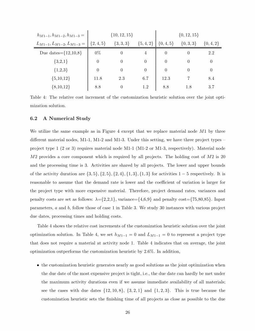
hM1−1, hM1−2, hM1−3 = {10, 12, 15} {0, 12, 15}LM1−1, LM1−2, LM1−3 = {2, 4, 5} {3, 3, 3} {5, 4, 2} {0, 4, 5} {0, 3, 3} {0, 4, 2}

Due dates={12,10,8} 0% 0 4 0 0 2.2

{3,2,1} 0 0 0 0 0 0

{1,2,3} 0 0 0 0 0 0

{5,10,12} 11.8 2.3 6.7 12.3 7 8.4

{8,10,12} 8.8 0 1.2 8.8 1.8 3.7

Table 4: The relative cost increment of the customization heuristic solution over the joint opti-

mization solution.

6.2 A Numerical Study

We utilize the same example as in Figure 4 except that we replace material node M1 by three

different material nodes, M1-1, M1-2 and M1-3. Under this setting, we have three project types –

project type 1 (2 or 3) requires material node M1-1 (M1-2 or M1-3, respectively). Material node

M2 provides a core component which is required by all projects. The holding cost of M2 is 20

and the processing time is 3. Activities are shared by all projects. The lower and upper bounds

of the activity duration are {3, 5}, {2, 5}, {2, 4}, {1, 3}, {1, 3} for activities 1 − 5 respectively. It is

reasonable to assume that the demand rate is lower and the coefficient of variation is larger for

the project type with more expensive material. Therefore, project demand rates, variances and

penalty costs are set as follows: λ={2,2,1}, variance={4,6,9} and penalty cost={75,80,85}. Input

parameters, a and b, follow those of case 1 in Table 3. We study 30 instances with various project

due dates, processing times and holding costs.

Table 4 shows the relative cost increments of the customization heuristic solution over the joint

optimization solution. In Table 4, we set hM1−1 = 0 and LM1−1 = 0 to represent a project type

that does not require a material at activity node 1. Table 4 indicates that on average, the joint

optimization outperforms the customization heuristic by 2.6%. In addition,

• the customization heuristic generates nearly as good solutions as the joint optimization when

the due date of the most expensive project is tight, i.e., the due date can hardly be met under

the maximum activity durations even if we assume immediate availability of all materials;

see the cases with due dates {12, 10, 8}, {3, 2, 1} and {1, 2, 3}. This is true because the

customization heuristic sets the finishing time of all projects as close as possible to the due

26

hM1−1, hM1−2, hM1−3 = {10, 12, 15} {0, 12, 15}LM1−1, LM1−2, LM1−3 = {2, 4, 5} {3, 3, 3} {5, 4, 2} {0, 4, 5} {0, 3, 3} {0, 4, 2}

Due dates={12,10,8} 19% 18.3 8.4 19 18.3 10.3

{3,2,1} 1.1 1.2 1.1 1.1 1.2 1.2

{1,2,3} 1.1 1.1 1.1 1.1 1.1 1.1

{5,10,12} 1.2 9.8 5.2 2.4 5.6 4.2

{8,10,12} 3.7 13.5 10.7 3.7 10.6 8.8

Table 5: The relative cost increment of the sequential heuristic solution over customization heuristic

solution.

date of the most expensive project to reduce penalty cost. Although some additional inventory

costs can be generated from less expensive projects, these costs are not significant and so the

customization heuristic performs well in these cases.

• The customization heuristic is less effective when due dates are not tight and vary substantially

across projects; e.g., the cases with due dates {5, 10, 12} and {8, 10, 12}. This is expected

because the customization heuristic assigns identical activity finishing times for activities

across project types, while the joint optimization allows them to be different.

• Among the cases with non-tight due dates, we observe that the customization heuristic tends

to be less effective in the case where the due date and customized material lead times follow the

same pattern than in the case where they follow a reverse pattern, see, e.g., the example with

due date {8, 10, 12} and customized material lead times {2, 4, 5} and the example with due

date {8, 10, 12} and material lead times {5, 4, 2}. This is true because in the former, the joint

optimization can delay the finishing times of the longer lead time projects to take advantage

of the pattern but the customization heuristic cannot, which leads to poor performance of the

customization heuristic. In the latter case, neither joint optimization nor the customization

heuristic can take advantage of the pattern, and thus their performance gaps are small.

Now we compare the customization heuristic with the sequential heuristic in Table 5:

• Similar to non-customized cases in §5, when the due dates of all projects are tight, the savings

of the customization heuristic diminish.

• The savings from the customization heuristic seem greater when the customized materials

27

have identical lead times. This is true because the customization heuristic tends to perform

as well as the joint optimization in these cases.

7 Conclusion and Discussion

In this paper, we focus on strategic planning of recurrent projects and their material supplies over an

extended period of time. Motivated by recent trends in various project-oriented industries to shift

the cost and time from on-site project activities to off-site supply chain activities, and to modularize

and standardize parts and products, we identify the common features for a class of problems where

supply chain and project management decisions are intertwined. We present a modeling framework,

the PDSC, to jointly plan for supply chain lead times and project resource/schedule.

Our basic model, although simplified and ignores issues such as non-consumable resources con-

straints, acyclic network structure and economies of scales, captures the trade-off between material

lead times and activity duration/schedule for recurrent projects. We show that the joint optimiza-

tion of material lead times and project activities can result in substantial savings relative to the

practice that makes material supply and project decisions separately. We extend the basic model

to include material customization and develop insights on the conditions under which the savings

are significant.

We can extend the basic PDSC model in various ways:

• Activity Customization. In addition to material customization, a company can also cus-

tomize projects by activities. Activity customization introduces challenges to the solution

algorithm because for projects requiring different sets of activities, it may not be reasonable

to set identical finishing times for common activities across projects. Furthermore, their due

dates can be very different. Thus, the customization heuristic developed in §6 is not ade-

quate. To solve activity customization problems, one can use metaheuristics such as branch

and bound or simulated annealing. One can also approximate the objective function by

piecewise linear functions which lead to mixed integer programming problems.

• Non-consumable Resource Constraints. Our basic model implicitly considers non-

consumable resource (labor/machine) via the direct cost but ignores the resource constraints.

For recurrent projects, non-consumable resource constraints are important because a com-

pany’s cannot easily change such resources significantly over projects (such as crane, quality

28

engineers). In addition, such constraints model the flexibility of project planning and schedul-

ing at different levels of material availability. While such constraints can be easily incorporated

in the PDSC model, they can significantly complicate the solution algorithm. Given the fact

that such resource constraints are extensively studied in the project management, one option

is to solve these problems using integer programming and/or heuristics.

• Acyclic PDSC. Acyclic PDSC arises when a material is required by multiple activities. For

acyclic PDSCs, a similar mathematical model (as the basic model in §3) can be formulated

but the dynamic programming algorithm does not work. Such a problem can be solved by

metaheuristics.

• Economies of Scale in Material Ordering. The economies of scale (batch-size require-

ments, minimum order quantities) in ordering are important factors for material management.

Economies of scale not only introduce additional challenges in managing the material net-

work, but also affect project decisions and cost. This is true because given the same inventory

cost, the committed lead time tends to be longer with larger batch-size requirements, which

mandates shorter activity durations and/or alters the project schedule to meet the due date.

Thus, models that include economies of scale can provide a more realistic treatment to balance

the trade-off between supply chain costs and project costs.

References

[1] Abdullah, A. M., I. G. Vicridge (1999). Best practice for multi-project management in the

construction industry. In Proceedings COBRA. RICS Foundation. 169-179.

[2] Aquilano, N. J., D. E. Smith (1980). A formal set of algorithms for project scheduling with

critical path method-material requirements planning. Journal of Operations Management, 1,

57-67.

[3] Axsater, S. (2006) Inventory Control, 2nd Edition. Springer, New York, NY.

[4] Blismas, N., W. Sher, A. Thorpe, A. Baldwin (2004). A typology for clients’ multi-project

environments. Construction Management and Economics, 22, 357-371.

[5] Brown, K., T. G. Schmitt, R. J. Schonberger, S. Dennis (2004). Quadrant Homes applies lean

concepts in a project environment. Interfaces, 34, 442-450.

29

[6] Cox, A., P. Ireland (2002) Managing construction supply chains: the common sense approach.

Engineering, Construction and Architectural Management, 9, 409-418.

[7] Cox, A., M. Townsend (1998). Strategic Procurement in Construction. Thomas Telford Pub-

lishing, London.

[8] Dodin, B., A. A. Elimam (2001). Integrated project scheduling and material planning with

variable activity duration and rewards. IIE Transactions, 33, 1005-1018.

[9] Graves, S. C., S. P. Willems (2000). Optimizing strategic safety stock placement in supply

chains. Manufacturing and Service Operations Management. 2, 68-83.

[10] Graves, S. C., S. P. Willems (2003a). Erratum: Optimizing strategic safety stock placement

in supply chains. Manufacturing and Service Operations Management. 5, 176-177.

[11] Graves, S. C., S. P. Willems (2003b). Supply chain design: safety stock placement and supply

chain configuration, in A. G. de Kok and S. C. Graves, eds, Handbooks in Operations Research

and Management Science Vol. 11, Supply Chain Management: Design, Coordination and

Operation. North-Holland Publishing Company, Amsterdam, The Netherlands.

[12] Graves, S. C., S. P. Willems (2005). Optimizing the Supply Chain Configuration for New

Products. Management Science, 51, 11651180.

[13] Gunasekaran, A., E.W.T. Ngai (2004). Build-to-order supply chain management: a literature

review and framework for development. Journal of Operations Management, 23, 423-451.

[14] Hastak, M., M. Syal (2004). Building process optimization with supply chain management

in the manufactured housing industry. Proceedings of the NSF Housing Research Agenda

Workshop, Feb. 12-14, 2004, Orlando, FL. Eds. Syal, M., Hastak, M., and Mullens, M. Vol.

2, Focus Group 1, 13-18.

[15] Jozefowska, J., Jan Weglarz (2006). Perspectives in Modern Project Scheduling. Springer; 1st

edition.

[16] Kerwin, K. (2005). BW 50: A new blueprint at Pulte Homes. BusinessWeek, October 3rd,

2005.

[17] McKenna, M., H. Wilczynskiv (2005). Supply chain lessons can save capital projects.

http://www.strategy-business.com/press/enewsarticle/enews033105.

30

[18] Nahmias, S. (2005). Production and operations analysis, 5th Edition. MCGraw-Hill Irwin.

Boston.

[19] O’Brien, W. J., K. London, R. Vrijhoef (2002). Construction supply chain modeling: a re-

search review and interdisciplinary research agenda. Proceedings IGLC-10, 1-19. August 2002,

Gramado, Brazil.

[20] Ozdamar, L., G. Ulusoy (1995). A survey on the resource-constrained project scheduling

problem. IIE Transactions, 27, 574-586.

[21] Pinedo, M. (2005). Planning and Scheduling in Manufacturing and Services. Springer New

York, NY.

[22] Porteus, E. L. (2002). Foundations of Stochastic Inventory Theory. Stanford University Press,

California.

[23] Simchi-Levi, D., Y. Zhao (2005). Safety stock positioning in supply chains with stochastic

lead times. Manufacturing & Service Operations Management 7, 295-318.

[24] Simchi-Levi, D., Y. Zhao (2007). Three generic methods for evaluating stochastic multi-

echelon inventory systems. Working Paper. Rutgers University, Newark, NJ.

[25] Smith-Danials, D. E., N. J. Aquilano (1984). Constrained resource project scheduling subject

to material constraints. Journal of Operations Management, 4, 369-388.

[26] Smith-Daniels, D. E., V. L. Smith-Daniels (1987). Optimal project scheduling with materials

ordering. IIE Transactions, 19, 122-129.

[27] Stevenson, M., L.C. Hendry, B.G. Kingsman (2005). A review of production planning and

control: the applicability of key concepts to the make-to-order industry. International Journal

of Production Research, 43, 869-898.

[28] Tommelein, I. D., K. D. Walsh, J. C. Hershauer (2003). Improving Capital Projects Supply

Chain Performance. Research Report No. 172-11, Construction Industry Institute, Austin,

TX, 241 pp.

[29] Vaidyanathan, K., G. Howell (2007). Construction supply chain maturity model – conceptual

framework. Proceedings IGLC-15, 170-180. July 2007, Michigan, USA.

31

[30] Vrijhoef, R., L. Koskela (2000). Roles of supply chain management in construction. European

Journal of Purchasing and Supply Chain Management. 6, 169-178.

[31] Vrijhoef, R., H. de Ridder (2006). Applying systems thinking to supply chain integration in

construction. International CIB Symposium: Construction in the 21st Century – Local and

Global Challenges. October 2006, Rome, Italy.

[32] Walsh, K. D., J. C. Hershauer, I. D. Tommelein, T. A. Walsh (2004). Strategic positioning

of inventory to match demand in a capital projects supply chain. Journal of Construction

Engineering and Management, ASCE / November/December, 818-826.

[33] Yeo, K. T., J. H. Ning (2002). Integrating supply chain and critical chain concepts in

engineering-procure-construct (EPC) projects. International Journal of Project Management,

20, 253-262.

[34] Zipkin, P (2000). Foundations of Inventory Management. McGraw Hill, Boston.

32