Embed Size (px)
Citation preview

IFT preprint 19/2004
Chiral and magnetic rotationin atomic nuclei studied within
self-consistent mean-field methods
Przemys law Olbratowski
Instytut Fizyki Teoretycznej, Warszawa, Uniwersytet Warszawski
Institut de Recherches Subatomiques, Strasbourg,Universite Louis Pasteur de Strasbourg I,Institut National de Physique Nucleaire et de Physique de Particules
email: [email protected], http: www.fuw.edu.pl/~polbrat
A Ph.D. thesis prepared in collaboration between the Warsaw University, Poland,and the Louis Pasteur University, France, thanks to a scholarship from the FrenchGovernment. This work was supported in part by the Polish Committee for ScientificResearch (KBN) and by the Foundation for Polish Science (FNP).
Supervisors:Jacek Dobaczewski Instytut Fizyki Teoretycznej, WarszawaJerzy Dudek Institut de Recherches Subatomiques, Strasbourg
Referees:Wojciech Satu la Instytut Fizyki Teoretycznej, WarszawaJan Styczen Instytut Fizyki Jadrowej
im. H. Niewodniczanskiego, KrakowJohann Bartel Institut de Recherches Subatomiques, StrasbourgHubert Flocard Centre de Spectrometrie Nucleaire
et Spectrometrie de Masse, Orsay
Warsaw/Strasbourg, July 21, 2004


Wierz tym, ktorzy szukaja prawdy,i nie dowierzaj tym, ktorzy ja znalezli.
Andre Gide
Moim Rodzicom


Podziekowania Pragne podziekowac mojemu promotorowi, prof. Jackowi Dobaczew-skiemu, za przyjecie mnie pod swa opieke w Instytucie Fizyki Teoretycznej w Warsza-wie, propozycje tematyki pracy naukowej, bezcenna pomoc w rozwijaniu narzedzi nu-merycznych, ktorymi sie pos lugiwa lem, za poswiecana mi ciagle uwage, oraz za wnikliwakorekte moich publikacji i niniejszej pracy.
Remerciements Je tiens a remercier mon co-directeur de these, prof. Jerzy Dudek,de m’avoir accueilli a l’Institut de Recherches Subatomiques a Strasbourg, d’avoir surveillecontinuellement mon travail scientifique, et d’avoir attentivement lu et corrige mes pub-lications et ma these de doctorat.

Streszczenie Jednym z zastosowan metod sredniego pola w fizyce jadrowej jest obecniebadanie egzotycznych symetrii jader atomowych. Wiaze sie to w szczegolnosci z analiza rotacjijader woko l osi pochylonej wzgledem osi g lownych rozk ladu masy w modelu Tilted-Axis Crank-ing (TAC). Niniejsza praca przedstawia jedne z pierwszych obliczen TAC wykonanych metodamiw pe lni samozgodnymi. Zastosowano w niej metode Hartree’ego-Focka z dwucia lowym oddzia- lywaniem efektywnym Skyrme’a. Stworzono program komputerowy pozwalajacy na lamaniewszystkich symetrii przestrzennych rozwiazania. Jako pierwsze zastosowanie przeprowadzonoobliczenia dla pasm magnetycznych w 142Gd oraz chiralnych w 130Cs, 132La, 134Pr i 136Pm.Ich wystepowanie zwiazane jest odpowiednio z nowym mechanizmem lamania symetrii sfe-rycznej oraz ze spontanicznym lamaniem symetrii chiralnej. Samozgodne rozwiazania w 142Gdpotwierdzaja istotna role mechanizmu shears w tworzeniu ca lkowitego momentu pedu. Zgodnoscz danymi doswiadczalnymi nie jest jednak zadowalajaca, prawdopodobnie wskutek nieuwzgled-nienia korelacji par lub przeszacowania deformacji. Wyniki w 132La stanowia pierwszy w pe lnisamozgodny dowod, ze rotacja jadrowa moze przybierac charakter chiralny. Wykazano, ze ro-tacja chiralna moze wystepowac tylko powyzej pewnej krytycznej czestosci obrotu. Sprawdzo-no tez, ze cz lony pola sredniego Skyrme’a nieparzyste wzgledem odwrocenia czasu nie majajakosciowego wp lywu na wyniki.
Resume Une des applications recentes des methodes de champ moyen en physique nucleaireest l’etude des symetries exotiques du noyau. Cette problematique est reliee, en particulier, al’analyse de la rotation nucleaire autour d’un axe incline par rapport aux axes principaux de ladistribution de masse dans le modele dit de Tilted-Axis Cranking (TAC). Cette these presentel’un des premiers calculs TAC effectues dans le cadre de methodes entierement auto-coherentes.La methode Hartree-Fock avec l’interaction effective a deux corps de Skyrme a ete utilisee. Uncode numerique a ete ecrit qui permet de briser toutes les symetries spatiales des solutions.Comme premiere application, des calculs pour les bandes magnetiques dans 142Gd et pour lesbandes chirales dans 130Cs, 132La, 134Pr et 136Pm ont ete effectues. L’existence de ces bandesest due a un nouveau mecanisme de brisure de la symetrie spherique, et de brisure spontanee dela symetrie chirale, respectivement. Les solutions auto-coherentes dans 142Gd confirment le roleimportant du mecanisme shears dans la generation du moment angulaire. Pourtant, l’accordavec les donnees experimentales n’est pas satisfaisant, probablement a cause de l’omission descorrelations d’appariement dans les calculs ou de la possible surestimation de la deformation.Les resultats obtenus dans 132La constituent la premiere preuve entierement auto-coherente quela rotation nucleaire peut acquerir un caractere chiral. Il a ete demontre que la rotation chiralene peut avoir lieu qu’au-dessus d’une certaine frequence angulaire critique. Il a ete egalementverifie que les termes du champ moyen de Skyrme impair par rapport au renversement du tempsn’ont pas d’influence qualitative sur les resultats.
Abstract Currently, one application of the mean-field methods in nuclear physics is theinvestigation of exotic nuclear symmetries. This is related, in particular, to the study of nuclearrotation about an axis tilted with respect to the principal axes of the mass distribution in theTilted-Axis Cranking (TAC) model. The present work presents one of the first TAC calculationsperformed within fully self-consistent methods. The Hartree-Fock method with the Skyrmeeffective two-body interaction has been used. A computer code has been developed that allowsfor the breaking of all spatial symmetries of the solution. As a first application, calculationsfor the magnetic bands in 142Gd and for the chiral bands in 130Cs, 132La, 134Pr, and 136Pmhave been carried out. The appearance of those bands is due to a new mechanism of breakingthe spherical symmetry and to the spontaneous breaking of the chiral symmetry, respectively.The self-consistent solutions for 142Gd confirm the important role of the shears mechanism ingenerating the total angular momentum. However, the agreement with experimental data isnot satisfactory, probably due to the lack of the pairing correlations in the calculations or tothe possibly overestimated deformation. The results obtained for 132La constitute the first fullyself-consistent proof that the nuclear rotation can attain a chiral character. It has been shownthat the chiral rotation can only exist above a certain critical angular frequency. It has also beenchecked that the terms of the Skyrme mean field odd under the time reversal have no qualitativeinfluence on the results.

Contents
1 Introduction 7
2 Magnetic and chiral rotations 112.1 Magnetic rotation . . . . . . . . . . . . . . . . . . . . . . . . . . . . . . . . 112.2 Chiral rotation . . . . . . . . . . . . . . . . . . . . . . . . . . . . . . . . . 17
3 Theoretical tools 273.1 Spontaneous symmetry breaking . . . . . . . . . . . . . . . . . . . . . . . . 273.2 Symmetries and rotational bands . . . . . . . . . . . . . . . . . . . . . . . 293.3 Tilted-Axis Cranking . . . . . . . . . . . . . . . . . . . . . . . . . . . . . . 313.4 The HF time-odd coupling constants . . . . . . . . . . . . . . . . . . . . . 353.5 Symmetry-unrestricted mean-field codes . . . . . . . . . . . . . . . . . . . 383.6 The program hfodd (v2.05c) . . . . . . . . . . . . . . . . . . . . . . . . . 39
4 Properties of the h11/2 valence nucleons 434.1 Symmetries of the non-rotating solutions . . . . . . . . . . . . . . . . . . . 434.2 Single-particle PAC Routhians for triaxial nuclei . . . . . . . . . . . . . . . 444.3 DT
2 -symmetric mean field . . . . . . . . . . . . . . . . . . . . . . . . . . . . 454.4 Influence of the pairing correlations . . . . . . . . . . . . . . . . . . . . . . 47
5 Hartree-Fock shears results in 142Gd 495.1 Previous studies in 142Gd . . . . . . . . . . . . . . . . . . . . . . . . . . . . 495.2 HF solutions in 142Gd . . . . . . . . . . . . . . . . . . . . . . . . . . . . . . 515.3 The shears mechanism in 142Gd . . . . . . . . . . . . . . . . . . . . . . . . 535.4 Comparison with experiment . . . . . . . . . . . . . . . . . . . . . . . . . . 56
6 Hartree-Fock chiral results 596.1 Previous studies in 130Cs, 132La, 134Pr, and 136Pm . . . . . . . . . . . . . . 596.2 HF minima in the N = 75 isotones . . . . . . . . . . . . . . . . . . . . . . 616.3 PAC calculations . . . . . . . . . . . . . . . . . . . . . . . . . . . . . . . . 636.4 Classical model and the critical frequency . . . . . . . . . . . . . . . . . . 666.5 Classical estimates of the critical frequency . . . . . . . . . . . . . . . . . . 706.6 Planar HF bands . . . . . . . . . . . . . . . . . . . . . . . . . . . . . . . . 726.7 Search for the chiral HF solutions . . . . . . . . . . . . . . . . . . . . . . . 746.8 Self-consistent chiral Skyrme-HF solutions . . . . . . . . . . . . . . . . . . 776.9 Comparison with experiment . . . . . . . . . . . . . . . . . . . . . . . . . . 78
1

2 CONTENTS
7 Conclusions and outlook 85
A Invariance of the time-even density 87
B Alignment and decoupling vectors 89
C Technical details of the calculations 93
D Single-particle Routhians 95
List of Figures
2.1 Magnetic bands throughout the nuclear chart. . . . . . . . . . . . . . . . . 122.2 The shears mechanism. . . . . . . . . . . . . . . . . . . . . . . . . . . . . . 132.3 Chirality of nuclear rotation. . . . . . . . . . . . . . . . . . . . . . . . . . . 182.4 Trajectory of the spin vector along a chiral band. . . . . . . . . . . . . . . 202.5 A generic chiral band from PRM. . . . . . . . . . . . . . . . . . . . . . . . 21
4.1 Influence of pairing on the single-particle alignments. . . . . . . . . . . . . 48
5.1 Partial level scheme of 142Gd. . . . . . . . . . . . . . . . . . . . . . . . . . 505.2 TRS for the ground state in 142Gd. . . . . . . . . . . . . . . . . . . . . . . 505.3 HF TAC results for the shears closing in 142Gd. . . . . . . . . . . . . . . . 545.4 Deformation along the HF shears band in 142Gd. . . . . . . . . . . . . . . . 555.5 HF and experimental energies for the πh2
11/2 νh−211/2 shears band in 142Gd. . 56
6.1 Level schemes of chiral doublets in N = 75 isotones. . . . . . . . . . . . . . 606.2 Alignments of the valence h11/2 nucleons in 132La from HF PAC. . . . . . . 636.3 Total alignments in 130Cs, 132La, 134Pr, 136Pm from HF PAC. . . . . . . . . 656.4 The classical model for the chiral rotation. . . . . . . . . . . . . . . . . . . 666.5 The ω(µ) dependence for the classical model and the classical planar and
chiral solutions in the ω space. . . . . . . . . . . . . . . . . . . . . . . . . . 696.6 Spins and energies for the planar and chiral bands in the classical model. . 706.7 Spin vectors of the valence h11/2 nucleons along the HF planar bands in
the N = 75 isotones. . . . . . . . . . . . . . . . . . . . . . . . . . . . . . . 736.8 HF and classical trajectory of ω along the planar bands in the N = 75
isotones. . . . . . . . . . . . . . . . . . . . . . . . . . . . . . . . . . . . . . 756.9 Perturbative search for HF chiral solutions. . . . . . . . . . . . . . . . . . . 766.10 Trajectory of ω along the HF chiral bands in 132La, compared to the clas-
sical predictions. . . . . . . . . . . . . . . . . . . . . . . . . . . . . . . . . 786.11 Alignments of the h11/2 proton on the principal axes in the HF chiral solu-
tion in 132La. . . . . . . . . . . . . . . . . . . . . . . . . . . . . . . . . . . 796.12 Experimental I(ω) dependence for the chiral bands in N = 75 isotones. . . 806.13 HF, classical and experimental energies for the chiral bands in 130Cs. . . . 816.14 HF, classical and experimental energies for the chiral bands in 132La. . . . 826.15 HF, classical and experimental energies for the chiral bands in 134Pr, 136Pm. 83
D.1 Axial Routhians in 142Gd for SLy4 force with N time-odd fields. . . . . . . 96D.2 Planar Routhians in 142Gd with N time-odd fields. . . . . . . . . . . . . . 97
3
4 LIST OF FIGURES
D.3 Planar Routhians in 142Gd with G time-odd fields. . . . . . . . . . . . . . . 98D.4 Planar Routhians in 142Gd with T time-odd fields. . . . . . . . . . . . . . . 99D.5 Axial Routhians in 130Cs for SLy4 force with N time-odd fields. . . . . . . 100D.6 Proton Axial Routhians in 132La for SLy4 force with N time-odd fields. . . 101D.7 Neutron Axial Routhians in 132La for SLy4 force with N time-odd fields. . 102D.8 Axial Routhians in oblate 134Pr for SLy4 force with N time-odd fields. . . . 103D.9 Axial Routhians in triaxial 134Pr for SkM* force with N time-odd fields. . . 104D.10 Axial Routhians in oblate 136Pm for SLy4 force with N time-odd fields. . . 105D.11 Axial Routhians in triaxial 136Pm for SkM* force with N time-odd fields. . 106D.12 Planar and Chiral Routhians in 132La with N time-odd fields. . . . . . . . 107D.13 Planar and Chiral Routhians in 132La with G time-odd fields. . . . . . . . . 108D.14 Planar and Chiral Routhians in 132La with T time-odd fields. . . . . . . . . 109
List of Tables
2.1 Experimental and theoretical investigations of candidate chiral bands. . . . 242.2 Continuation of Table 2.1. . . . . . . . . . . . . . . . . . . . . . . . . . . . 25
3.1 Types of rotational bands and symmetries of the nucleus. . . . . . . . . . . 303.2 HF time-odd coupling constants. . . . . . . . . . . . . . . . . . . . . . . . 383.3 Symmetry patterns allowed in the code hfodd. . . . . . . . . . . . . . . . 41
5.1 Single-particle configurations for the HF solutions in 142Gd. . . . . . . . . . 52
6.1 Single-particle configurations for the HF solutions in the N = 75 isotones. . 626.2 Deformations, parameters of the classical model, and critical frequencies
and spins for the N = 75 isotopes. . . . . . . . . . . . . . . . . . . . . . . . 71
5

6 LIST OF TABLES
Chapter 1
Introduction
The phenomenon of spontaneous symmetry breaking is a leading theme of a multitude ofquantum effects. For instance, it is due to the spontaneous breaking of the particle-numbersymmetry that superconducting condensates appear in metals. Spontaneous breaking oc-curs if a system in its endeavor to attain the minimal energy chooses a symmetry-violatingstate even though the underlying interactions are invariant under the concerned symme-try. Nevertheless, it is the nature of the interactions that determines which symmetriesare broken and under which conditions. Therefore, study of symmetry-violating statesbrings one closer to understanding the interactions - the most fundamental goal in physics.
In the nuclear structure physics, one important example of spontaneous symmetrybreaking is the existence of deformed nuclei. Like for molecules, violation of the sphericalinvariance leads to the appearance of rotational excitations, which manifest themselvesin specific sequences of levels, the rotational bands. Depending on the conservation orviolation of other symmetries, like the plane reflection, those bands can have differentstructures. Recently, two novel types of bands have been observed experimentally, thathave challenged the theoretical models. They are called magnetic and chiral bands.
The peculiarity of the magnetic structures is that, contrary to all the previously knownrotational bands, they appear in nuclei whose charge distribution is nearly spherical, whichcan be inferred from the very weak electric quadrupole transitions. On the other hand,magnetic dipole transitions, to which the bands owe their name, are strong. Thus, thebands constitute the first evidence for the breaking of the spherical symmetry by a largedipole moment, which, in turn, is produced by highly asymmetric current distributions.In the absence of charge deformation, no collective rotation is possible, and the magneticbands also entail a new mechanism of generating the angular momentum, in which valencenucleons play a crucial role. The angular momenta of the valence particles align coherentlyalong one direction, and those of the valence holes along a perpendicular direction. Thespin of the levels in the band is produced by gradual alignment of the two angular momentavectors. This has been dubbed shears mechanism, because it resembles the closing of apair of shears used for cutting the sheep wool. The magnetic bands were first observed inearly 1990s, and more that 130 such structures have been found so far.
The chiral bands have the form of doublets of bands lying very close in energy. Sinceother hypotheses failed to reproduce the vanishing energy splitting between them, it hasbeen suggested that the doublets are due to the possible existence of two enantiomeric(left- or right-handed) forms of the nucleus. The chiral bands are observed mainly in well-
7

8 CHAPTER 1. INTRODUCTION
deformed nuclei, in which there is one valence proton particle and one valence neutronhole in an orbital of high angular momentum. The former drives the nucleus towardselongated shapes, while the latter towards oblate ones. The interplay of these oppositetendencies may result in a shape resembling a triaxial ellipsoid. In the triaxially deformednucleus, the particle and hole align their angular momenta along the short and long axesof the density distribution, respectively. Moreover, the moment of inertia with respectto the medium axis is the largest, which favors the collective rotation around that axis.Thus, the total angular momentum vector has non-zero components on all the three axes,and those component vectors can form either a left-handed or a right-handed system.This means, according to the original Kelvin’s definition, that the system is chiral, onlythat its chirality is related to the handedness of angular momenta rather than of positionvectors. First chiral bands were identified about the year of 2000, and ten odd occurrencesare known now.
The chiral rotation has been successfully examined within the phenomenological Par-ticle-Rotor Model, in which the nucleus is represented by a rigid core with a few valencenucleons coupled to it. However, the very concept of both the shears mechanism androtational chirality came from considerations within the mean-field cranking approach,which is one of the most fundamental methods in the nuclear structure physics. In thisapproximation, each nucleon is moving independently in a rotating potential that repre-sents an averaged interaction with other nucleons. The main point about the mean-fielddescription of the two considered phenomena is that it must allow for rotation aboutan axis that does not coincide with any principal axis of the mass distribution; such avariant of the cranking model is called Tilted-Axis Cranking (TAC). Before the interestin magnetic and chiral bands arose, only rotations about principal axes were considered,so addressing the new effects required an upgrade of the existing numerical tools. Afirst TAC code was written by Frauendorf [Fra93a]; it used a phenomenological meanpotential to describe the properties of the valence particles, and the nuclear liquid-dropmodel to account for some bulk properties of the nucleus. A great deal of experimentaldata, mainly on magnetic bands, has been analyzed by using that code, and generally agood agreement was obtained. As far as more fundamental methods are concerned, onlyone magnetic band in 84Rb has been studied by Madokoro et al. [Mad00a] within theRelativistic-Mean-Field method.
Although the phenomenological model of Frauendorf has led to a remarkable suc-cess, a more fundamental description requires self-consistent methods, in which the meanpotential is indeed generated from averaging an effective two-body interaction with thenucleonic density. First of all, such an approach is capable to provide a strong test of thestability of the proposed shears and chiral configurations with respect to the core degreesof freedom. It is also necessary to take into account several important effects, like all kindsof polarization of the core by the valence particles and full minimization of the underly-ing energies with respect to all deformation variables, including the deformation of thecurrent and spin distributions. Application of self-consistent methods to the descriptionof the magnetic and chiral rotation is the subject of this PhD dissertation.
The author developed a code that can perform TAC calculations within the fullHartree-Fock (HF) method with the Skyrme effective interaction [Rin00a]. It is oneof the first existing tools of this kind, and allows for a study of many other effects; for
9
instance, it has already been used to calculate the time-reversal violating Schiff momentof 225Ra [Eng03a] in connection with the search for fundamental breaking of the T or CPsymmetry beyond the Standard Model. In the present work, the first Skyrme-HF TACsolutions were found. For the study of the shears bands, the nucleus of 142Gd was cho-sen. The HF results corroborated that an important portion of the angular momentumis generated by the shears mechanism, although the shape deformation is non-negligible,and the collective rotation of the core is also present. The chiral solutions were lookedfor in four N = 75 isotones, 130Cs, 132La, 134Pr, 136Pm, and found in the second one. Itwas established that the chiral rotation appears only above a certain critical value of theangular frequency. The origin of the critical frequency was explained in terms of a verysimple classical model, that provides a surprising agreement with the HF results.
In Chapter 2, an introduction to the physics of the magnetic and chiral bands is given,together with a review of the literature. Chapter 3 describes the theoretical tool usedin this work - the Skyrme-HF TAC method. Particular emphasis is put on the issue ofspontaneous symmetry breaking in rotational bands and on technical differences betweenthe self-consistent and phenomenological approaches. One aspect that can be studieduniquely within the self-consistent approach is the influence of the HF time-odd densitiesand fields on the shears and chiral solutions. The way this is investigated in the presentwork is also described in that Chapter. Finally, the code hfodd is presented. Therotational behavior of the nuclei here under study is determined, to a big extent, by thealignment properties of a few valence h11/2 nucleons. In Chapter 4, their basic featuresare established from standard (non-TAC) cranking calculations and from pure symmetryconsiderations. The Skyrme-HF results for the shears band in 142Gd are presented inChapter 5. Chapter 6 gives the planar and chiral solutions for the N = 75 isotones. There,the classical model is formulated, the expression for the critical frequency is derived, andits values are analyzed. Since the present calculations constitute the first application of theSkyrme-HF TAC method, several technical details on how the solutions were obtained arealso given in that Chapter. Chapter 7 summarizes the main conclusions from the presentwork, and outlines prospects for further research.

10 CHAPTER 1. INTRODUCTION
Chapter 2
Magnetic and chiral rotations
A classical rigid body can rotate uniformly only about the principal axes of its inertiatensor. However, already Riemann showed [Rie60a] that in liquids rotation about a tiltedaxis may take place if there is an intrinsic vortical motion. In a drop of nuclear matter,the nucleus, vorticity may arise from the presence of unpaired nucleons near the Fermilevel. The swirling vortices produce the single-particle (s.p.) angular momenta that takevarious directions and add to the collective rotation drawing the total spin away from theprincipal axes. It is the rotation about a tilted axis that breaks the signature and chiralsymmetries, and gives rise to the magnetic and chiral bands. The two phenomena showdifferent ways of coupling the s.p. spins to the collective rotation.
2.1 Magnetic rotation
In early 1990’s, very regular rotational bands were observed in several light lead isotopes[Bal92a, Cla92a, Kuh92a], and were initially mistaken for superdeformed structures. Butdetailed measurements showed that they had an unusual feature: weak E2 and strong M1transitions. To date, many more similar structures have been identified. They are calledmagnetic dipole or shears bands. This Section recapitulates their main characteristics andpresents the mechanisms that are believed to lie at their origin.
Taking into account the vast experimental evidence, one can enumerate the followingproperties that can be considered as a definition of the magnetic dipole bands:
• Levels in the band form the I+, (I +1)+, (I +2)+ or I−, (I +1)−, (I +2)− spin-paritysequence.
• Bands never start at spins less than about 10h, except for the lightest nuclides, andapproximately follow the regular rotational dependence of E ∼ I(I + 1).
• The E2 transitions within the band are very weak, with reduced probabilities B(E2)typically not exceeding ∼ 0.1 e2b2. In contrast, the values of B(M1) are exception-ally large, in the range of ∼ 2 − 10µN . They exhibit a characteristic fall withincreasing spin.
• The ratio J (2)/B(E2) assume the values of ∼ 100 h2MeV−1e−2b−2 that is roughlyan order of magnitude larger than for normal or superdeformed bands.
11
12 CHAPTER 2. MAGNETIC AND CHIRAL ROTATIONS
N
Z
2 8 20 28 50 82 126
28
20
28
50
82
114
f5/2
g9/2
d5/2 g7/2
h11/2
h9/2g 9
/2
d 5/2
g7/
2
h 11/
2
f 7/2
h9/
2
i 13/
2
f 5/2
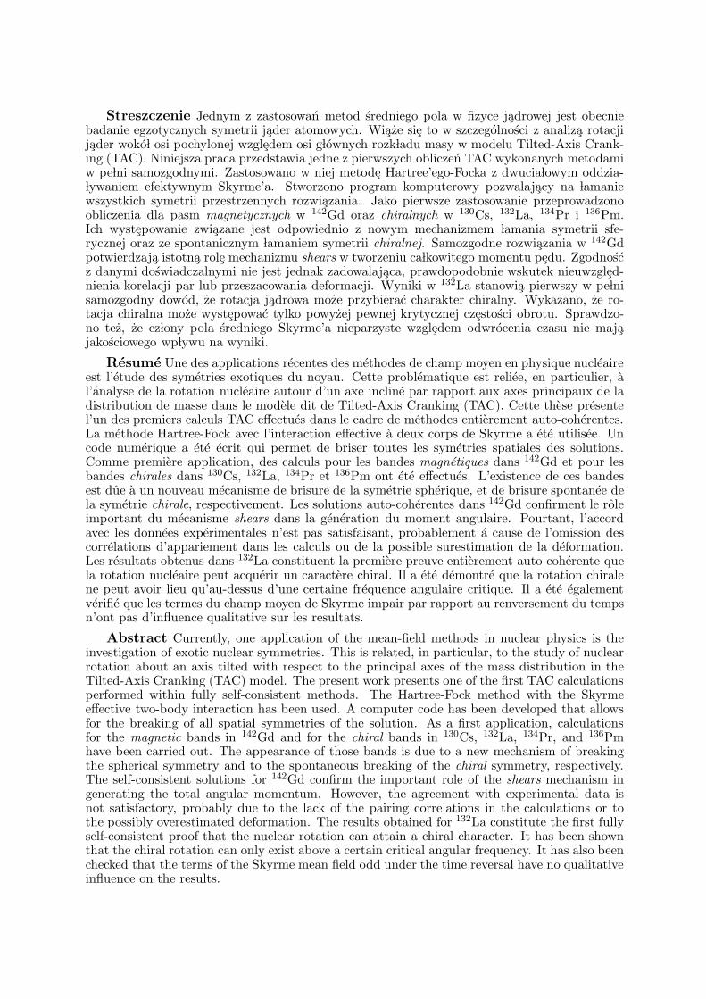
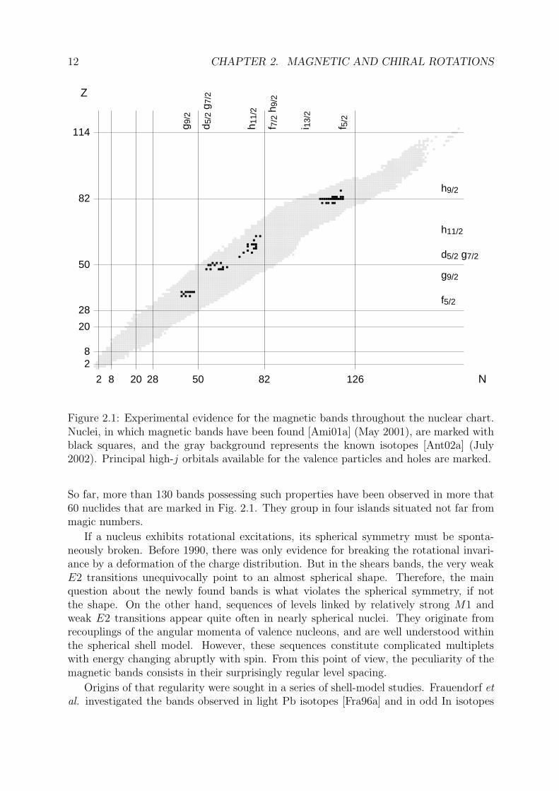
Figure 2.1: Experimental evidence for the magnetic bands throughout the nuclear chart.Nuclei, in which magnetic bands have been found [Ami01a] (May 2001), are marked withblack squares, and the gray background represents the known isotopes [Ant02a] (July2002). Principal high-j orbitals available for the valence particles and holes are marked.
So far, more than 130 bands possessing such properties have been observed in more that60 nuclides that are marked in Fig. 2.1. They group in four islands situated not far frommagic numbers.
If a nucleus exhibits rotational excitations, its spherical symmetry must be sponta-neously broken. Before 1990, there was only evidence for breaking the rotational invari-ance by a deformation of the charge distribution. But in the shears bands, the very weakE2 transitions unequivocally point to an almost spherical shape. Therefore, the mainquestion about the newly found bands is what violates the spherical symmetry, if notthe shape. On the other hand, sequences of levels linked by relatively strong M1 andweak E2 transitions appear quite often in nearly spherical nuclei. They originate fromrecouplings of the angular momenta of valence nucleons, and are well understood withinthe spherical shell model. However, these sequences constitute complicated multipletswith energy changing abruptly with spin. From this point of view, the peculiarity of themagnetic bands consists in their surprisingly regular level spacing.
Origins of that regularity were sought in a series of shell-model studies. Frauendorf etal. investigated the bands observed in light Pb isotopes [Fra96a] and in odd In isotopes
2.1. MAGNETIC ROTATION 13
jp
jh
j
µp
µh
µ
a)
jp
jh
j
µp
µh
µ
b)
jp
jh
j
µp
µh
µ
c)
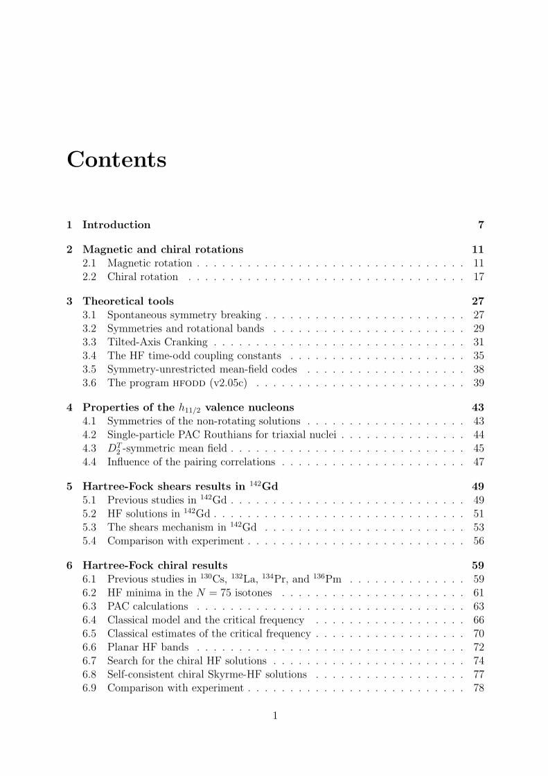
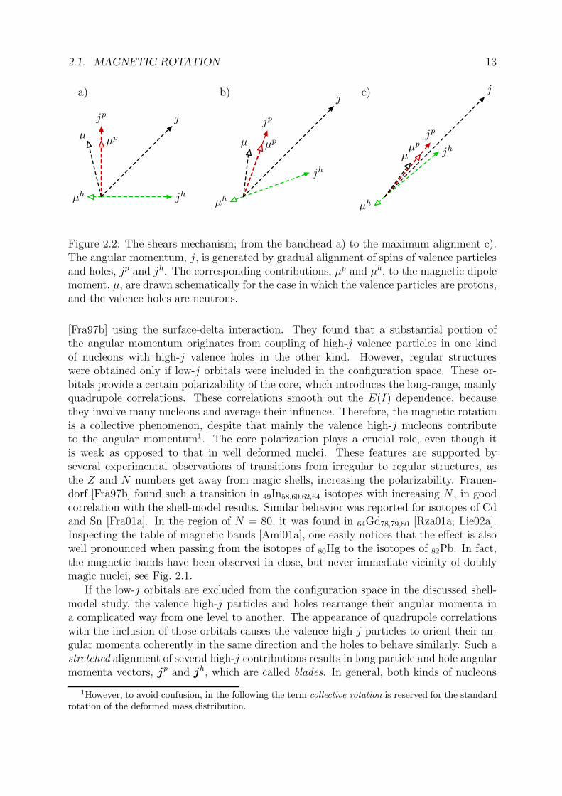
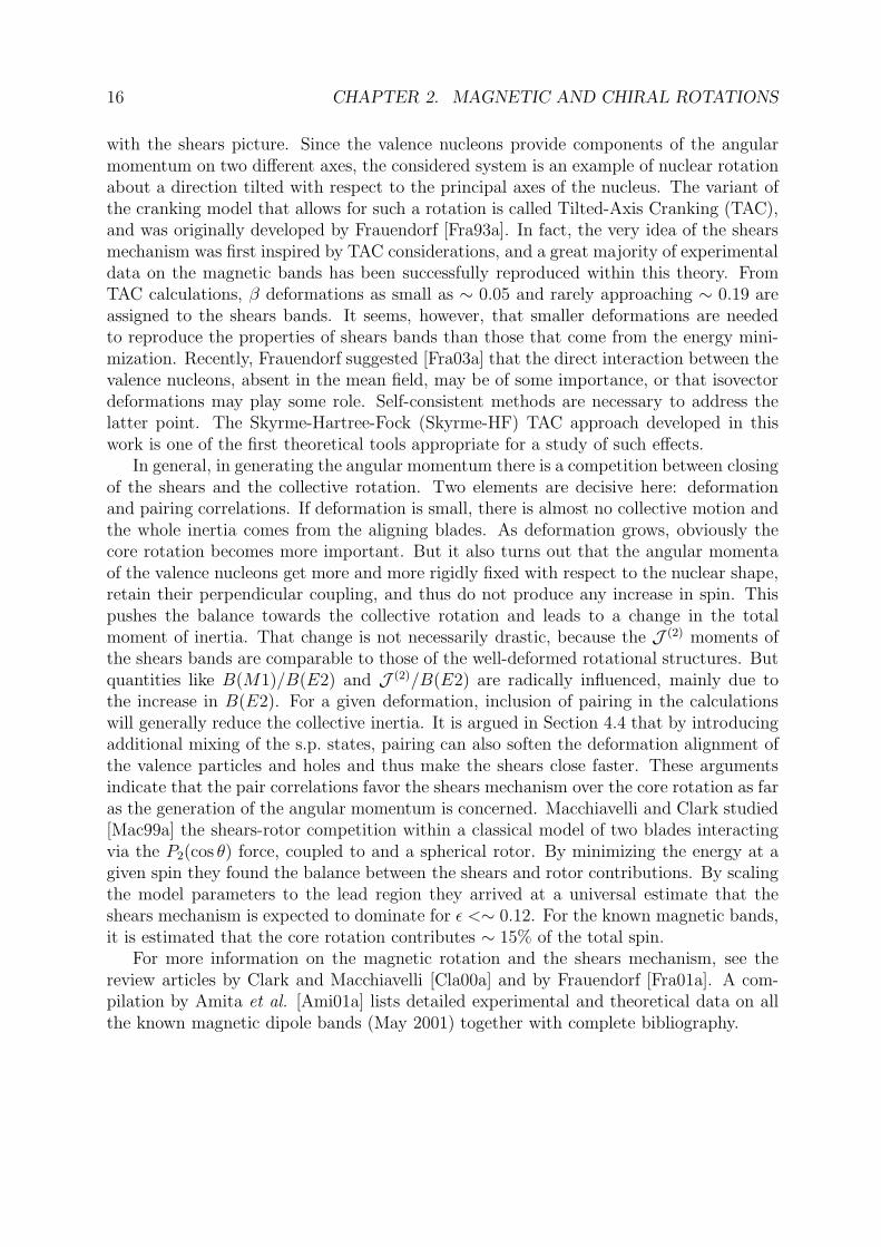
Figure 2.2: The shears mechanism; from the bandhead a) to the maximum alignment c).The angular momentum, j, is generated by gradual alignment of spins of valence particlesand holes, jp and jh. The corresponding contributions, µp and µh, to the magnetic dipolemoment, µ, are drawn schematically for the case in which the valence particles are protons,and the valence holes are neutrons.
[Fra97b] using the surface-delta interaction. They found that a substantial portion ofthe angular momentum originates from coupling of high-j valence particles in one kindof nucleons with high-j valence holes in the other kind. However, regular structureswere obtained only if low-j orbitals were included in the configuration space. These or-bitals provide a certain polarizability of the core, which introduces the long-range, mainlyquadrupole correlations. These correlations smooth out the E(I) dependence, becausethey involve many nucleons and average their influence. Therefore, the magnetic rotationis a collective phenomenon, despite that mainly the valence high-j nucleons contributeto the angular momentum1. The core polarization plays a crucial role, even though itis weak as opposed to that in well deformed nuclei. These features are supported byseveral experimental observations of transitions from irregular to regular structures, asthe Z and N numbers get away from magic shells, increasing the polarizability. Frauen-dorf [Fra97b] found such a transition in 49In58,60,62,64 isotopes with increasing N , in goodcorrelation with the shell-model results. Similar behavior was reported for isotopes of Cdand Sn [Fra01a]. In the region of N = 80, it was found in 64Gd78,79,80 [Rza01a, Lie02a].Inspecting the table of magnetic bands [Ami01a], one easily notices that the effect is alsowell pronounced when passing from the isotopes of 80Hg to the isotopes of 82Pb. In fact,the magnetic bands have been observed in close, but never immediate vicinity of doublymagic nuclei, see Fig. 2.1.
If the low-j orbitals are excluded from the configuration space in the discussed shell-model study, the valence high-j particles and holes rearrange their angular momenta ina complicated way from one level to another. The appearance of quadrupole correlationswith the inclusion of those orbitals causes the valence high-j particles to orient their an-gular momenta coherently in the same direction and the holes to behave similarly. Such astretched alignment of several high-j contributions results in long particle and hole angularmomenta vectors, jp and jh, which are called blades. In general, both kinds of nucleons
1However, to avoid confusion, in the following the term collective rotation is reserved for the standardrotation of the deformed mass distribution.
14 CHAPTER 2. MAGNETIC AND CHIRAL ROTATIONS
can contribute to each blade, but in most cases the particles are protons and the holesare neutrons. At the bandhead, the two blades turn out to form an angle of nearly 90
(Fig. 2.2a). Since the proton and neutron effective g-factors, gπ and gν , have oppositesigns, the perpendicular coupling also gives rise to a large magnetic dipole moment, µ,with a significant component, µ⊥, perpendicular to the total spin, j, (Fig. 2.2a). Thisis the source of the strong M1 transitions, because the reduced probability B(M1) isproportional to µ2
⊥. The perpendicular coupling of jp and jh has been confirmed by anexperimental determination of the effective g-factor in the bandhead of a shears band in193Pb [Chm97a]. In the band, jp and jh align towards each other, retaining their constantlengths. In this way, the total spin increases, while µ⊥ decreases, causing the observeddrop-off in the M1 strength (Fig. 2.2b). Assuming the geometry shown in Fig. 2.2, Mac-chiavelli and Clark [Mac98a] calculated the B(M1) values for the magnetic bands in 198Pband 199Pb as proportional to µ2
⊥, and obtained a good overall agreement with experiment.Obviously, the maximum spin that can be generated in such a way approximately equalsthe sum of jp and jh, whereas µ⊥ and B(M1) vanish when the maximum alignment isachieved (Fig. 2.2c). This mode of generating the angular momentum and the magneticmoment was originally proposed by Frauendorf [Fra93a], and was then dubbed shearsmechanism [Bal94a], because it resembles the closing of a pair of shears used for cuttingthe sheep wool.
In view of the important role of the quadrupole polarization, the magnetic bands havebeen investigated within approaches that take that polarization into account in a modelway. In [Mac98b] and also in [Mac98a, Mac98c, Mac99a], Macchiavelli and Clark used theparticle-vibration theory [Boh75a], considering the coupling of the valence high-j particlesand holes to the quadrupole vibrations of the nuclear shape about a spherical equilibrium.They postulated the stretched coupling of the constituent angular momenta in each bladeand treated all the valence particles as one particle with spin jp and all the valence holes asone hole with spin jh. In the second order of the perturbation series, the particle-vibrationcoupling gives rise to an effective interaction between the valence nucleons. It takes theform of the second-order Legendre polynomial, P2(cos ϑ), where ϑ is the angle betweenthe position vectors of the valence particle and hole. It was shown in [Boh53a] that in thelimit of high angular momenta the expectation value of the interaction P2(cos ϑ) in thestate |jpjhj〉 becomes proportional to P2(cos θ), where, this time, θ is the angle betweenjp and jh, the shears angle. Actually, these results were obtained in such a regime of theparticle-vibration theory, in which there already exist a static quadrupole polarizationof the core. Therefore, it is not surprising that they could also be derived within themean-field approximation. Frauendorf considered [Fra01a] the quadrupole-quadrupolemodel with some simplifications similar to that made by Macchiavelli and Clark. Hepresumed that in both protons and neutrons the ensemble of the valence nucleons canbe treated as one object with constant quadrupole tensor and mean angular momentumpointing along one of its principal axes. Under these assumptions and with the aid of theaddition theorem for spherical harmonics, the quadrupole-quadrupole interaction betweenthe valence particles and holes transforms directly into the form of P2(cos θ). He alsopostulated that the valence nucleons are the only source of polarization of the otherwisespherical core and that the core energy depends quadratically on the induced quadrupolemoment. The core defined in this way only modifies the strength of the P2(cos θ) force.
2.1. MAGNETIC ROTATION 15
It comes both from the particle-vibration theory and from the mean-field quadrupole-quadrupole model that for the relevant particle-hole case the coupling constant of theP2(cos θ) interaction is positive. Since the polynomial P2(cos θ) itself has a minimum atθ = 90, the perpendicular coupling at the bandhead is reproduced. These facts lie at theorigin of the following popular picture that can be found in the literature. States belongingto high-j orbitals have doughnut-like shapes with mean angular momenta pointing alongthe symmetry axis of such a density distributions. Therefore, the right-angle orientationof the two spin vectors at the bandhead corresponds to a minimal spatial overlap ofthe particle and hole wave-functions. One usually says that this is because the particle-hole interaction is repulsive, and tends to minimize the overlap. This reasoning maybe misleading, because it overlooks the core, whereas the P2(cos θ) interaction describesprecisely the influence of the core polarization, and does not have the sense of a directforce.
With the P2(cos θ) interaction at hand, one can address the fundamental question ofhow the energy changes with spin in a shears band. Although the quadrupole correlationssmooth out the E(I) dependence, the shears mechanism of generating the angular mo-mentum is substantially different from that occurring for the collective rotation, and it isnot obvious whether it should also lead to the rotational-like behavior of E ∼ I(I + 1).In their model study, Macchiavelli and Clark assumed that the P2(cos θ) force is the onlysource of the energy change along the band and that the whole angular momentum comesfrom the shears closing, that is, I = j. Under these assumptions, the energy, E, of a levelbelonging to a shears band has the form of P2(cos θ),
E ∼ 3 cos2 θ − 1
2, (2.1)
whereas from the shears geometry shown in Fig. 2.2 one easily obtains
cos θ =I2 − (jp)2 − (jh)2
2jpjh. (2.2)
Substitution of (2.2) to (2.1) yields a fourth-order E(I) dependence, and the fourth-order term is not only a correction, because the quadratic term has a negative sign. Forgiven values of jp and jh, the shears angle, θ, can be extracted from the experimentalspins according to (2.2) and the obtained dependence of E(θ) can be compared with theform (2.1). Such an analysis was done for 198,199Pb [Mac98b] and 142Gd [Rza01a], givinga satisfactory agreement with (2.1). The fourth-order dependence translates into non-constant moments of inertia. This aspect was exploited in [Mac98c], where a qualitativeagreement with the moments of inertia for a band in 197Pb was found.
The important role of the quadrupole polarization and the quasi-classical behaviorof the angular momenta of the high-j nucleons make the magnetic rotation suitable forthe mean-field description within the cranking model. In this approach, the alignmentproperties of the valence particles and holes are governed by the deformation of the meanpotential. It turns out that the high-j particles and holes align their mean angular mo-mentum vectors, jp and jh, on the short and on the long axis of the deformed nucleus,respectively, giving the perpendicular coupling at the bandhead. With increasing rota-tional frequency, the two blades gradually align towards the axis of rotation, in agreement
16 CHAPTER 2. MAGNETIC AND CHIRAL ROTATIONS
with the shears picture. Since the valence nucleons provide components of the angularmomentum on two different axes, the considered system is an example of nuclear rotationabout a direction tilted with respect to the principal axes of the nucleus. The variant ofthe cranking model that allows for such a rotation is called Tilted-Axis Cranking (TAC),and was originally developed by Frauendorf [Fra93a]. In fact, the very idea of the shearsmechanism was first inspired by TAC considerations, and a great majority of experimentaldata on the magnetic bands has been successfully reproduced within this theory. FromTAC calculations, β deformations as small as ∼ 0.05 and rarely approaching ∼ 0.19 areassigned to the shears bands. It seems, however, that smaller deformations are neededto reproduce the properties of shears bands than those that come from the energy mini-mization. Recently, Frauendorf suggested [Fra03a] that the direct interaction between thevalence nucleons, absent in the mean field, may be of some importance, or that isovectordeformations may play some role. Self-consistent methods are necessary to address thelatter point. The Skyrme-Hartree-Fock (Skyrme-HF) TAC approach developed in thiswork is one of the first theoretical tools appropriate for a study of such effects.
In general, in generating the angular momentum there is a competition between closingof the shears and the collective rotation. Two elements are decisive here: deformationand pairing correlations. If deformation is small, there is almost no collective motion andthe whole inertia comes from the aligning blades. As deformation grows, obviously thecore rotation becomes more important. But it also turns out that the angular momentaof the valence nucleons get more and more rigidly fixed with respect to the nuclear shape,retain their perpendicular coupling, and thus do not produce any increase in spin. Thispushes the balance towards the collective rotation and leads to a change in the totalmoment of inertia. That change is not necessarily drastic, because the J (2) moments ofthe shears bands are comparable to those of the well-deformed rotational structures. Butquantities like B(M1)/B(E2) and J (2)/B(E2) are radically influenced, mainly due tothe increase in B(E2). For a given deformation, inclusion of pairing in the calculationswill generally reduce the collective inertia. It is argued in Section 4.4 that by introducingadditional mixing of the s.p. states, pairing can also soften the deformation alignment ofthe valence particles and holes and thus make the shears close faster. These argumentsindicate that the pair correlations favor the shears mechanism over the core rotation as faras the generation of the angular momentum is concerned. Macchiavelli and Clark studied[Mac99a] the shears-rotor competition within a classical model of two blades interactingvia the P2(cos θ) force, coupled to and a spherical rotor. By minimizing the energy at agiven spin they found the balance between the shears and rotor contributions. By scalingthe model parameters to the lead region they arrived at a universal estimate that theshears mechanism is expected to dominate for ε <∼ 0.12. For the known magnetic bands,it is estimated that the core rotation contributes ∼ 15% of the total spin.
For more information on the magnetic rotation and the shears mechanism, see thereview articles by Clark and Macchiavelli [Cla00a] and by Frauendorf [Fra01a]. A com-pilation by Amita et al. [Ami01a] lists detailed experimental and theoretical data on allthe known magnetic dipole bands (May 2001) together with complete bibliography.
2.2. CHIRAL ROTATION 17
2.2 Chiral rotation
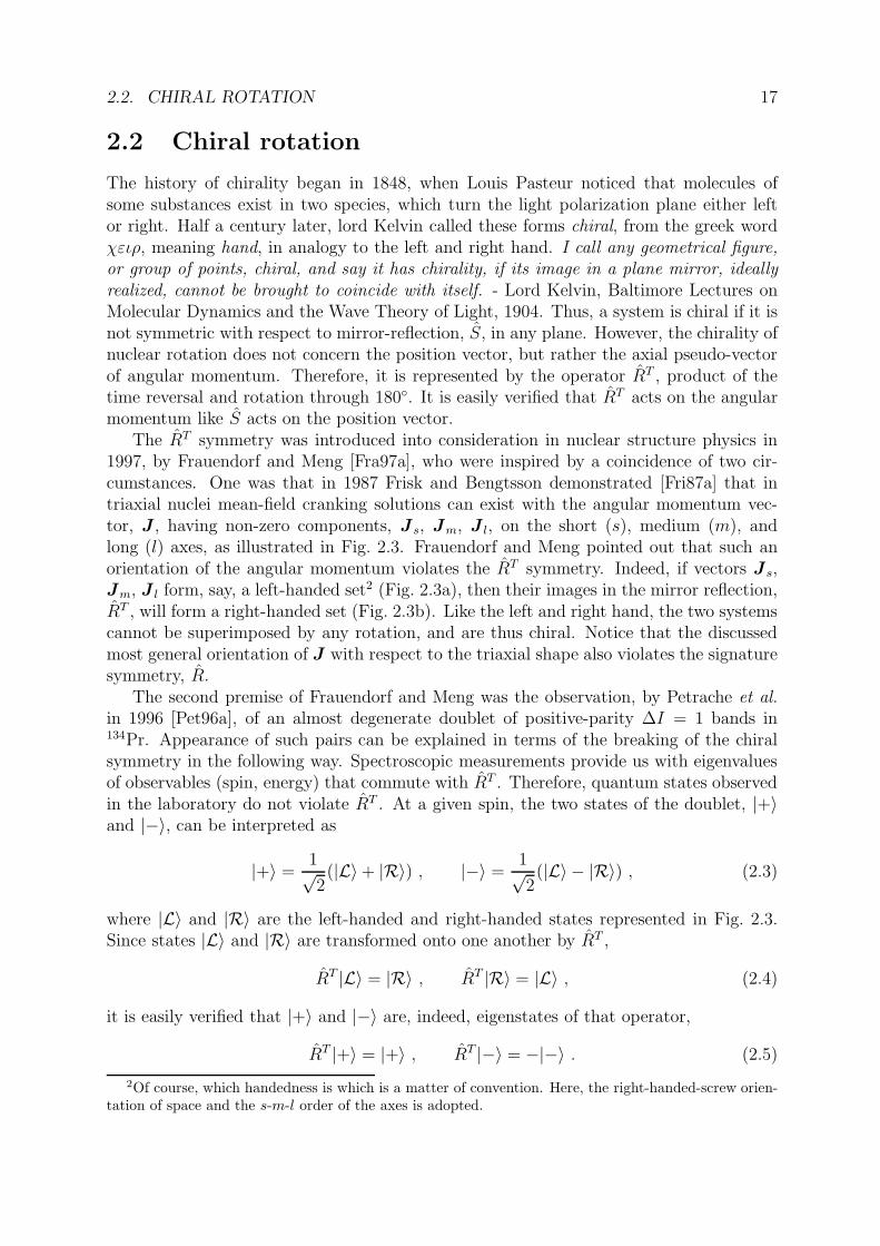
The history of chirality began in 1848, when Louis Pasteur noticed that molecules ofsome substances exist in two species, which turn the light polarization plane either leftor right. Half a century later, lord Kelvin called these forms chiral, from the greek wordχειρ, meaning hand, in analogy to the left and right hand. I call any geometrical figure,or group of points, chiral, and say it has chirality, if its image in a plane mirror, ideallyrealized, cannot be brought to coincide with itself. - Lord Kelvin, Baltimore Lectures onMolecular Dynamics and the Wave Theory of Light, 1904. Thus, a system is chiral if it isnot symmetric with respect to mirror-reflection, S, in any plane. However, the chirality ofnuclear rotation does not concern the position vector, but rather the axial pseudo-vectorof angular momentum. Therefore, it is represented by the operator RT , product of thetime reversal and rotation through 180. It is easily verified that RT acts on the angularmomentum like S acts on the position vector.
The RT symmetry was introduced into consideration in nuclear structure physics in1997, by Frauendorf and Meng [Fra97a], who were inspired by a coincidence of two cir-cumstances. One was that in 1987 Frisk and Bengtsson demonstrated [Fri87a] that intriaxial nuclei mean-field cranking solutions can exist with the angular momentum vec-tor, J , having non-zero components, J s, Jm, J l, on the short (s), medium (m), andlong (l) axes, as illustrated in Fig. 2.3. Frauendorf and Meng pointed out that such anorientation of the angular momentum violates the RT symmetry. Indeed, if vectors J s,Jm, J l form, say, a left-handed set2 (Fig. 2.3a), then their images in the mirror reflection,RT , will form a right-handed set (Fig. 2.3b). Like the left and right hand, the two systemscannot be superimposed by any rotation, and are thus chiral. Notice that the discussedmost general orientation of J with respect to the triaxial shape also violates the signaturesymmetry, R.
The second premise of Frauendorf and Meng was the observation, by Petrache et al.in 1996 [Pet96a], of an almost degenerate doublet of positive-parity ∆I = 1 bands in134Pr. Appearance of such pairs can be explained in terms of the breaking of the chiralsymmetry in the following way. Spectroscopic measurements provide us with eigenvaluesof observables (spin, energy) that commute with RT . Therefore, quantum states observedin the laboratory do not violate RT . At a given spin, the two states of the doublet, |+〉and |−〉, can be interpreted as
|+〉 =1√2
(|L〉+ |R〉) , |−〉 =1√2
(|L〉 − |R〉) , (2.3)
where |L〉 and |R〉 are the left-handed and right-handed states represented in Fig. 2.3.Since states |L〉 and |R〉 are transformed onto one another by RT ,
RT |L〉 = |R〉 , RT |R〉 = |L〉 , (2.4)
it is easily verified that |+〉 and |−〉 are, indeed, eigenstates of that operator,
RT |+〉 = |+〉 , RT |−〉 = −|−〉 . (2.5)
2Of course, which handedness is which is a matter of convention. Here, the right-handed-screw orien-tation of space and the s-m-l order of the axes is adopted.
18 CHAPTER 2. MAGNETIC AND CHIRAL ROTATIONS
Jl=jh
Js=jp Jm=RJ
|L〉 Jl=jh
Js=jp
Jm=RJ
|R〉
Figure 2.3: Triaxially deformed nucleus with the angular momentum, J , having non-zerocomponents, J s, Jm, J l, on the short (s), medium (m), and long (l) axis. The left panel,|L〉, shows the left-handed orientation of those three vectors, and the right panel, |R〉,shows the right-handed orientation. The components J s, Jm, J l originate from the spinof the valence particle, jp, from the collective angular momentum, R, and from the spinof the valence hole, jh, respectively.
They are also orthogonal3. The nuclear many-body Hamiltonian, H , is invariant underRT , and therefore the states |L〉 and |R〉 have equal mean energies. At the same time,the matrix element of H between those states is, in general, non-zero, i.e.,
〈L|H|L〉 = 〈R|H|R〉 = E , |〈L|H|R〉| = ∆ 6= 0 . (2.6)
As a consequence, the energies of the laboratory states, |+〉 and |−〉, read
〈+|H|+〉 = E + ∆ , 〈−|H|−〉 = E −∆ . (2.7)
Their energy splitting is, of course, due to the interaction between the left- and right-handed states. One can see that doublet bands like those observed in 134Pr may beattributed to the breaking of the chiral symmetry.
One can thus suppose that the appearance of the doublet bands is connected to theexistence of triaxially deformed states with the angular momentum vector lying outsideany principal plane. Frauendorf and Meng pointed out that in odd-odd nuclei around134Pr such states can arise in the following way. In this region, a configuration is easilyavailable, in which one proton particle occupies the lowest substate of the h11/2 orbital,and simultaneously one neutron hole is left in the highest h11/2 substate. The formerdrives the nucleus towards elongated shapes, while the latter towards disc-like forms.The interplay of these opposite tendencies may yield stable triaxiality. In the triaxiallydeformed potential, the considered particle and hole align their angular momenta, jp andjh, along the short and long axis of the nucleus, respectively, providing the J s and J l
components of J . As expected from the hydrodynamical irrotational-flow model [Boh75a],the moment of inertia with respect to the medium axis is the largest, which energetically
3More precisely, they can be always made orthogonal by an appropriate choice of phases of the states|L〉 and |R〉.
2.2. CHIRAL ROTATION 19
favors the collective rotation about this direction. Thus, the component Jm comes fromthe collective angular momentum, R. This is illustrated in Fig. 2.3.
Since the first observation in 134Pr, about 12 similar structures have been found in odd-odd nuclei in the A ∼ 130 region. They are all attributed to the discussed configurationof πh1
11/2 νh−111/2. Recently, first observations of possibly chiral bands in the even-odd
135Nd [Zhu03a] and in the even-even 136Nd [Mer02a] were reported in the same region.There, the proposed active configurations are πh2
11/2 νh−111/2 and πh2
11/2 νh−111/2, respectively.
Peng, Meng, and Zhang predicted theoretically [Pen03a] that another island of chirality,associated mainly with the configuration πg1
9/2 νg−19/2, may exist around A ∼ 100. Indeed,
experimental work is underway for 102−106Rh [Sta03a] and gives promising results. It seemsthat a pair of bands found in 104Rh [Koi03b, Vam04a] provides the best known exampleof a chiral doublet, because the chiral partners are situated closest to each other. In thiscase, the πg−1
9/2 νh11/2 configuration is proposed. Latest lifetime measurements in 132La, by
Grodner et al. [Gro04a], provided the first direct information about the absolute B(E2)and B(M1) values in the chiral bands; see Section 6.1. A complete (January 2004) reviewof experimental and theoretical investigations of the chiral bands in particular nuclides isgiven in Tabs. 2.1 and 2.2. See also Fig. 6.1 for sample level schemes and Figs. 6.13–6.15for spin-energy plots.
Certainly, an important question about the observed doublet bands is whether thechiral rotation is the only possible explanation of their appearance. A more standardpicture would be that they are in fact four ∆I = 2 bands corresponding to the two signa-ture states of the two odd nucleons, one proton and one neutron. The energy separationbetween the bands would then be just the signature splitting. However, the calculatedsignature splitting turned out to be a few times larger than the observed distance [Sta01b].Also the possibility that the yrare partner band is a gamma-vibrational excitation builton the yrast band has been ruled out for the same reason. However, recently Pasternak[Pas04a] managed to reproduce all the three bands observed in 132La (see Section 6.1) ina very simple classical model that invokes only planar rotation. Yet, some of the modelparameters were fitted to each band separately.
Two theoretical tools have been used for the description of the chiral rotation: variousversions of the Particle-Rotor Model (PRM), originally developed by Bohr and Mottelson[Boh75a] and the mean-field Tilted Axis Cranking (TAC) model, which is discussed inSection 3.3 and used in this work. In the PRM approach, the nucleus is represented by arotating deformed structureless core and a few valence particles interacting with it, andpossibly among themselves. The valence nucleons are usually treated as pure particles orholes, while calculations with pairing appeared only recently [Koi03a]. The core is usuallytaken as a triaxial rigid quantum rotor (Davydov-Fillipov model [Dav58a]), characterizedby three moments of inertia, Js, Jm, Jl, and described by the Hamiltonian
Hrot =R2
s
2Js
+R2
m
2Jm
+R2
l
2Jl
, (2.8)
where Rs, Rm, Rl are the intrinsic-frame components of the core angular momentum. Inall available PRM studies, the moments of inertia, Jk, are calculated from the irrotational-
20 CHAPTER 2. MAGNETIC AND CHIRAL ROTATIONS
planar
chiral
towards axial
Js
Jl
Jm
jp
jh
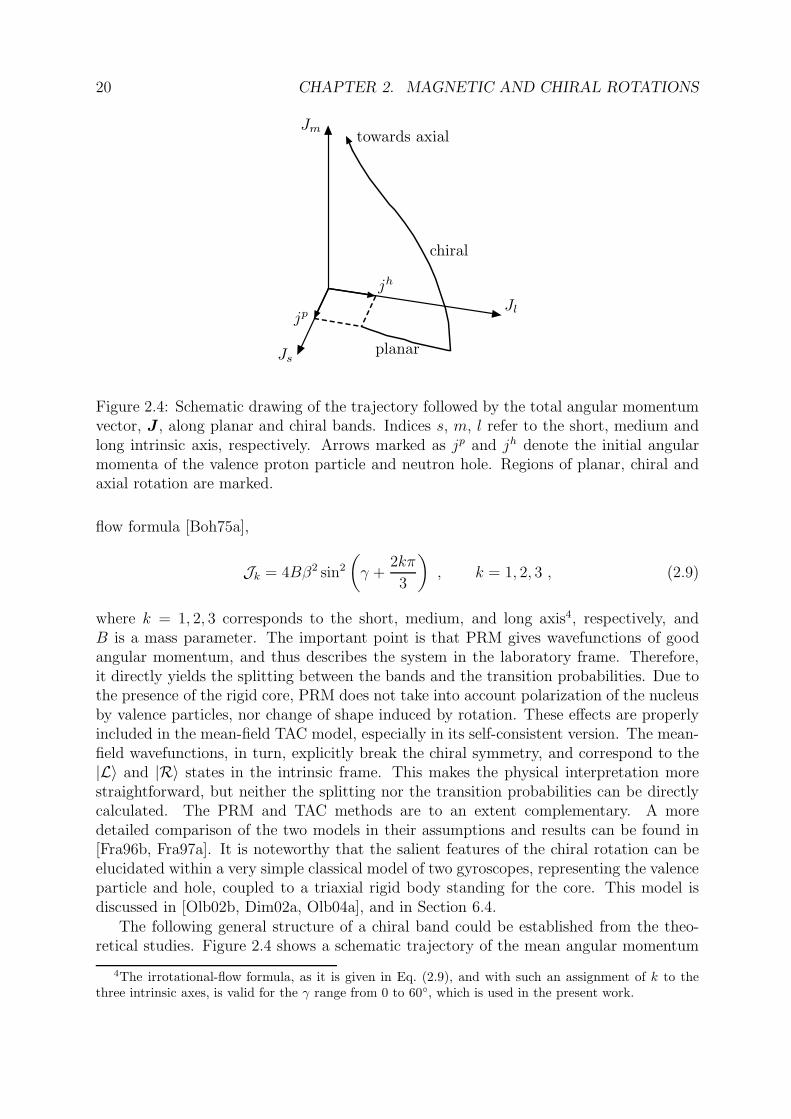
Figure 2.4: Schematic drawing of the trajectory followed by the total angular momentumvector, J , along planar and chiral bands. Indices s, m, l refer to the short, medium andlong intrinsic axis, respectively. Arrows marked as jp and jh denote the initial angularmomenta of the valence proton particle and neutron hole. Regions of planar, chiral andaxial rotation are marked.
flow formula [Boh75a],
Jk = 4Bβ2 sin2
(
γ +2kπ
3
)
, k = 1, 2, 3 , (2.9)
where k = 1, 2, 3 corresponds to the short, medium, and long axis4, respectively, andB is a mass parameter. The important point is that PRM gives wavefunctions of goodangular momentum, and thus describes the system in the laboratory frame. Therefore,it directly yields the splitting between the bands and the transition probabilities. Due tothe presence of the rigid core, PRM does not take into account polarization of the nucleusby valence particles, nor change of shape induced by rotation. These effects are properlyincluded in the mean-field TAC model, especially in its self-consistent version. The mean-field wavefunctions, in turn, explicitly break the chiral symmetry, and correspond to the|L〉 and |R〉 states in the intrinsic frame. This makes the physical interpretation morestraightforward, but neither the splitting nor the transition probabilities can be directlycalculated. The PRM and TAC methods are to an extent complementary. A moredetailed comparison of the two models in their assumptions and results can be found in[Fra96b, Fra97a]. It is noteworthy that the salient features of the chiral rotation can beelucidated within a very simple classical model of two gyroscopes, representing the valenceparticle and hole, coupled to a triaxial rigid body standing for the core. This model isdiscussed in [Olb02b, Dim02a, Olb04a], and in Section 6.4.
The following general structure of a chiral band could be established from the theo-retical studies. Figure 2.4 shows a schematic trajectory of the mean angular momentum
4The irrotational-flow formula, as it is given in Eq. (2.9), and with such an assignment of k to thethree intrinsic axes, is valid for the γ range from 0 to 60, which is used in the present work.
2.2. CHIRAL ROTATION 21
-2
-1
0
1
2
3
4
5
6
0 5 10 15 20 25
Ener
gy
[MeV
]
Spin [h]
pla
nar
chir
al axia
l
a)
0
5
10
15
20
25
-0.2 0 0.2 0.4 0.6 0.8
Spin
[h]
Rotational frequency [MeV/h]
planar
chiral
axial
b)
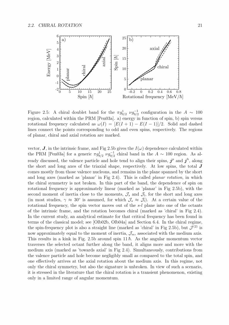
Figure 2.5: A chiral doublet band for the πg19/2 νg−1
9/2 configuration in the A ∼ 100
region, calculated within the PRM [Pen03a]. a) energy in function of spin, b) spin versusrotational frequency calculated as ω(I) = [E(I + 1) − E(I − 1)]/2. Solid and dashedlines connect the points corresponding to odd and even spins, respectively. The regionsof planar, chiral and axial rotation are marked.
vector, J , in the intrinsic frame, and Fig 2.5b gives the I(ω) dependence calculated withinthe PRM [Pen03a] for a generic πg1
9/2 νg−19/2 chiral band in the A ∼ 100 region. As al-
ready discussed, the valence particle and hole tend to align their spins, jp and jh, alongthe short and long axes of the triaxial shape, respectively. At low spins, the total J
comes mostly from those valence nucleons, and remains in the plane spanned by the shortand long axes (marked as ’planar’ in Fig 2.4). This is called planar rotation, in whichthe chiral symmetry is not broken. In this part of the band, the dependence of spin onrotational frequency is approximately linear (marked as ’planar’ in Fig 2.5b), with thesecond moment of inertia close to the moments, Js and Jl, for the short and long axes(in most studies, γ ≈ 30 is assumed, for which Js ≈ Jl). At a certain value of therotational frequency, the spin vector moves out of the s-l plane into one of the octantsof the intrinsic frame, and the rotation becomes chiral (marked as ’chiral’ in Fig 2.4).In the current study, an analytical estimate for that critical frequency has been found interms of the classical model; see [Olb02b, Olb04a] and Section 6.4. In the chiral regime,the spin-frequency plot is also a straight line (marked as ’chiral’ in Fig 2.5b), but J (2) isnow approximately equal to the moment of inertia, Jm, associated with the medium axis.This results in a kink in Fig. 2.5b around spin 11 h. As the angular momentum vectortraverses the selected octant further along the band, it aligns more and more with themedium axis (marked as ’towards axial’ in Fig 2.4). Simultaneously, contributions fromthe valence particle and hole become negligibly small as compared to the total spin, andone effectively arrives at the axial rotation about the medium axis. In this regime, notonly the chiral symmetry, but also the signature is unbroken. In view of such a scenario,it is stressed in the literature that the chiral rotation is a transient phenomenon, existingonly in a limited range of angular momentum.
22 CHAPTER 2. MAGNETIC AND CHIRAL ROTATIONS
Figure 2.4 shows the mean intrinsic-frame trajectory of the angular momentum vectoralong a chiral band. Classically, each point of that trajectory corresponds to a uniformrotation of the nucleus about a fixed direction, without any wobbling. Within the TACmodel, the trajectory follows the minimum of the energy surface with increasing rotationalfrequency. The two chiral partners can be viewed as two lowest quantum states in thepotential represented by that surface. In the single planar minimum existing at lowspins, the two states are interpreted as zero- and one-phonon excitations separated bya finite energy interval. They correspond to oscillations of the spin vector about theplanar equilibrium, which has a classical analogy in non-uniform rotations [Dim02a]. Inthe chiral regime, there is the left and right minimum, of equal depths. If the barrierbetween them is high enough, the two lowest eigenstates are nearly degenerate, and onecan talk about strong chiral symmetry breaking. For low barriers, the spin vector cantunnel between the minima, and the splitting between the band states is non-zero5. Thiskind of weak symmetry breaking has been dubbed chiral vibrations [Sta01b]. As theaxial rotation is approached, the weakened breaking of both the chiral symmetry andthe signature manifests itself, in particular, by the onset of the signature splitting. Thatsplitting is absent for the planar and chiral rotation, because the signature is stronglybroken in those modes. The above features appear clearly in the structure of the chiralband, as calculated in the PRM model. This can be seen from Fig. 2.5, showing the plotsof energy versus spin and spin versus rotational frequency.
The evolution from planar to chiral to axial finds a manifestation in the electromagneticproperties of the chiral bands, too. Those were examined in [Fra97a, Pen03a, Pen03b],mainly in the frame of the PRM model. For planar rotation, the transitions withineach partner band are strong, the transitions from the yrare to the yrast band are weak,and there are practically no decays in the opposite direction. In the chiral regime, allreduced probabilities assume moderate values, and the intraband and interband transitionstrengths are comparable. As the planar rotation is approached, the B(E2) within thetwo partners become equal and slowly increase, while the interband E2 decays disappear.The B(M1) show the characteristic odd-even staggering, absent at lower spins. Reference[Koi03a] gives a discussion of the staggering in B(M1)/B(E2) and B(M1)in/B(M1)out
(interband/intraband) in connection with the signature splitting and inversion.
The appearance of the chiral bands is considered a strong evidence for the existence oftriaxial deformations; certainly, the chiral geometry cannot occur in an axially symmetricnucleus. It is clear from the irrotational-flow formula (2.9) that γ = 30 gives the largestmoment of inertia with respect to the medium axis (Jm = 4Js = 4Jl) and thus favors theaplanar orientation of the angular momentum. The PRM study by Starosta et al. [Sta01a,Sta02a] showed that the value of γ practically does not influence the alignments of thevalence particle and hole on the short and long axis. However, those alignments are onlywell defined for sufficiently large β deformation. References [Sta01a, Sta02a] investigatedthe influence of γ and β on the mean value of the so-called orientation operator, σ =(jp × jh)R, which measures the aplanarity of jp, jh, and R, i.e., the degree of chirality,in a sense. The average value of σ increases with β and has a maximum for γ = 30. Thisis reflected in the splitting between the chiral partners, which decreases with β, and is
5However, in order to actually calculate the chiral splitting in such an approach, one would need themass parameter in addition to the potential surface, and such calculations have not been done.
2.2. CHIRAL ROTATION 23
minimal for γ = 30. However, it is known that the flow of matter in nuclei is not purelyirrotational, i.e., the curl of the velocity field is not exactly zero. Thus, the moments ofinertia may deviate from the irrotational-flow values (2.9) assumed in the PRM studies,especially if pairing is weak, and the dependence of the discussed observables on γ maynot be so straightforward.
As far as the mean-field methods are concerned, certainly taking into account theinteraction between the left- and right-handed minima would be desirable, preferablyin conjunction with the projection onto good chirality before variation. This would bethe first tool capable of calculating the chiral splitting and the transition probabilitiesin a fully microscopic way. In the PRM domain, efforts are being undertaken to includepairing in the calculations [Koi03a], to use γ-soft cores, and to take into account the directresidual interaction between the valence nucleons [Rai03a, Rai03b]. Such an interactionis supposed to be responsible for the stabilization of the chiral geometry in nuclei at thelimits of the islands of chirality. Experimentally, lifetime measurements would certainlybe of great use.
24 CHAPTER 2. MAGNETIC AND CHIRAL ROTATIONS
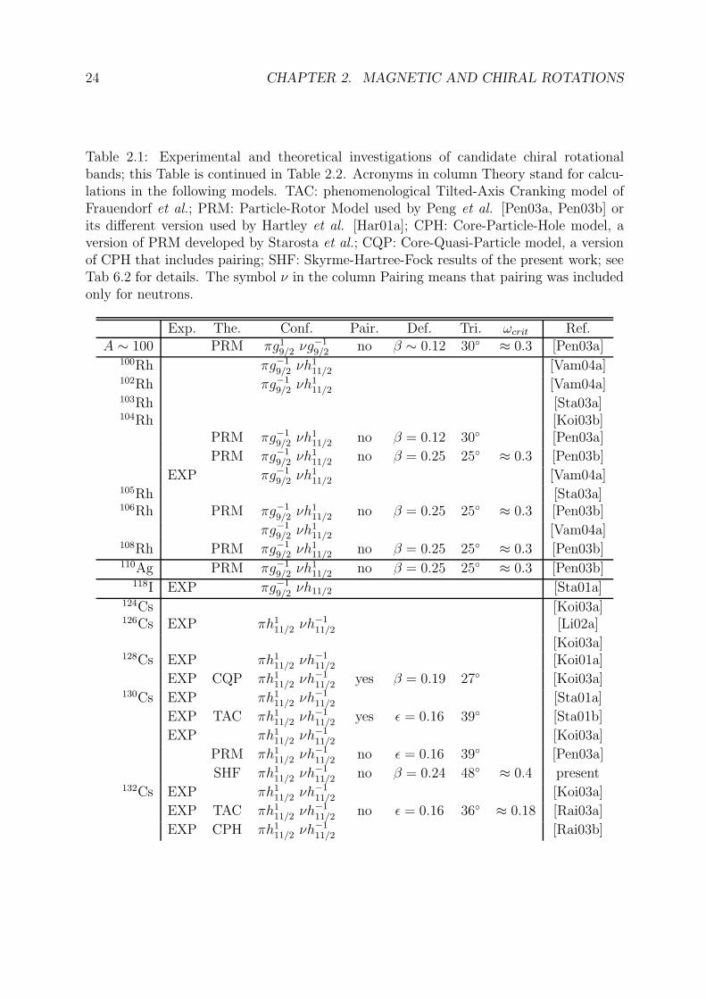
Table 2.1: Experimental and theoretical investigations of candidate chiral rotationalbands; this Table is continued in Table 2.2. Acronyms in column Theory stand for calcu-lations in the following models. TAC: phenomenological Tilted-Axis Cranking model ofFrauendorf et al.; PRM: Particle-Rotor Model used by Peng et al. [Pen03a, Pen03b] orits different version used by Hartley et al. [Har01a]; CPH: Core-Particle-Hole model, aversion of PRM developed by Starosta et al.; CQP: Core-Quasi-Particle model, a versionof CPH that includes pairing; SHF: Skyrme-Hartree-Fock results of the present work; seeTab 6.2 for details. The symbol ν in the column Pairing means that pairing was includedonly for neutrons.
Exp. The. Conf. Pair. Def. Tri. ωcrit Ref.A ∼ 100 PRM πg1
9/2 νg−19/2 no β ∼ 0.12 30 ≈ 0.3 [Pen03a]
100Rh πg−19/2 νh1
11/2 [Vam04a]102Rh πg−1
9/2 νh111/2 [Vam04a]
103Rh [Sta03a]104Rh [Koi03b]
PRM πg−19/2 νh1
11/2 no β = 0.12 30 [Pen03a]
PRM πg−19/2 νh1
11/2 no β = 0.25 25 ≈ 0.3 [Pen03b]
EXP πg−19/2 νh1
11/2 [Vam04a]105Rh [Sta03a]106Rh PRM πg−1
9/2 νh111/2 no β = 0.25 25 ≈ 0.3 [Pen03b]
πg−19/2 νh1
11/2 [Vam04a]108Rh PRM πg−1
9/2 νh111/2 no β = 0.25 25 ≈ 0.3 [Pen03b]
110Ag PRM πg−19/2 νh1
11/2 no β = 0.25 25 ≈ 0.3 [Pen03b]118I EXP πg−1
9/2 νh11/2 [Sta01a]124Cs [Koi03a]126Cs EXP πh1
11/2 νh−111/2 [Li02a]
[Koi03a]128Cs EXP πh1
11/2 νh−111/2 [Koi01a]
EXP CQP πh111/2 νh−1
11/2 yes β = 0.19 27 [Koi03a]130Cs EXP πh1
11/2 νh−111/2 [Sta01a]
EXP TAC πh111/2 νh−1
11/2 yes ε = 0.16 39 [Sta01b]
EXP πh111/2 νh−1
11/2 [Koi03a]
PRM πh111/2 νh−1
11/2 no ε = 0.16 39 [Pen03a]
SHF πh111/2 νh−1
11/2 no β = 0.24 48 ≈ 0.4 present132Cs EXP πh1
11/2 νh−111/2 [Koi03a]
EXP TAC πh111/2 νh−1
11/2 no ε = 0.16 36 ≈ 0.18 [Rai03a]
EXP CPH πh111/2 νh−1
11/2 [Rai03b]
2.2. CHIRAL ROTATION 25
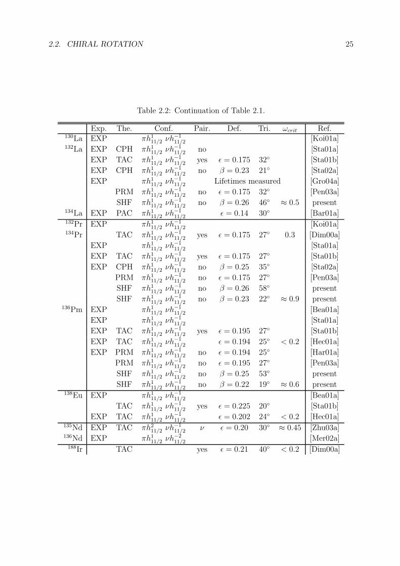
Table 2.2: Continuation of Table 2.1.
Exp. The. Conf. Pair. Def. Tri. ωcrit Ref.130La EXP πh1
11/2 νh−111/2 [Koi01a]
132La EXP CPH πh111/2 νh−1
11/2 no [Sta01a]
EXP TAC πh111/2 νh−1
11/2 yes ε = 0.175 32 [Sta01b]
EXP CPH πh111/2 νh−1
11/2 no β = 0.23 21 [Sta02a]
EXP πh111/2 νh−1
11/2 Lifetimes measured [Gro04a]
PRM πh111/2 νh−1
11/2 no ε = 0.175 32 [Pen03a]
SHF πh111/2 νh−1
11/2 no β = 0.26 46 ≈ 0.5 present134La EXP PAC πh1
11/2 νh−111/2 ε = 0.14 30 [Bar01a]
132Pr EXP πh111/2 νh−1
11/2 [Koi01a]134Pr TAC πh1
11/2 νh−111/2 yes ε = 0.175 27 0.3 [Dim00a]
EXP πh111/2 νh−1
11/2 [Sta01a]
EXP TAC πh111/2 νh−1
11/2 yes ε = 0.175 27 [Sta01b]
EXP CPH πh111/2 νh−1
11/2 no β = 0.25 35 [Sta02a]
PRM πh111/2 νh−1
11/2 no ε = 0.175 27 [Pen03a]
SHF πh111/2 νh−1
11/2 no β = 0.26 58 present
SHF πh111/2 νh−1
11/2 no β = 0.23 22 ≈ 0.9 present136Pm EXP πh1
11/2 νh−111/2 [Bea01a]
EXP πh111/2 νh−1
11/2 [Sta01a]
EXP TAC πh111/2 νh−1
11/2 yes ε = 0.195 27 [Sta01b]
EXP TAC πh111/2 νh−1
11/2 ε = 0.194 25 < 0.2 [Hec01a]
EXP PRM πh111/2 νh−1
11/2 no ε = 0.194 25 [Har01a]
PRM πh111/2 νh−1
11/2 no ε = 0.195 27 [Pen03a]
SHF πh111/2 νh−1
11/2 no β = 0.25 53 present
SHF πh111/2 νh−1
11/2 no β = 0.22 19 ≈ 0.6 present138Eu EXP πh1
11/2 νh−111/2 [Bea01a]
TAC πh111/2 νh−1
11/2 yes ε = 0.225 20 [Sta01b]
EXP TAC πh111/2 νh−1
11/2 ε = 0.202 24 < 0.2 [Hec01a]135Nd EXP TAC πh2
11/2 νh−111/2 ν ε = 0.20 30 ≈ 0.45 [Zhu03a]
136Nd EXP πh111/2 νh−2
11/2 [Mer02a]188Ir TAC yes ε = 0.21 40 < 0.2 [Dim00a]

26 CHAPTER 2. MAGNETIC AND CHIRAL ROTATIONS
Chapter 3
Theoretical tools
In this Chapter, some general information about the spontaneous symmetry breaking inthe mean field is recalled, mainly in the context of rotational bands. While the Tilted-Axis Cranking (TAC) method has already been widely discussed and used in its versionbased on phenomenological potentials, this work introduces one of its first applicationsto the self-consistent Hartree-Fock (HF) calculations. Therefore, the TAC basics arerecapitulated with particular emphasis on the differences between the phenomenologicaland self-consistent implementations. It is also described how the values of the time-oddcoupling constants of the HF energy functional are chosen in the present calculationsto investigate the role of the time-odd nucleonic densities and fields in the shears andchiral solutions. After a concise review of other computer codes capable of performingsymmetry-unrestricted mean-field calculations, the program hfodd, used in this work, ispresented.
3.1 Spontaneous symmetry breaking
This Section summarizes the basics of the HF method, and explains how the spontaneoussymmetry breaking intervenes in the mean-field approach.
The variational HF method consists, in its standard version, in minimizing the expec-tation value of the many-body Hamiltonian,
H = T + V , (3.1)
in the trial class of Slater determinants. Here, T is the kinetic energy, and V is theeffective two-body interaction. A Slater determinant, |Ψ〉, is uniquely characterized byits hermitian, projective density matrix,
ραβ = 〈Ψ|a+β aα|Ψ〉 . (3.2)
For a given density, one introduces the so-called s.p. Hamiltonian, h[ρ], which is thefunctional derivative of the energy, E = 〈Ψ|H|Ψ〉, with respect to the density,
h[ρ]βα =∂E
∂ραβ. (3.3)
27

28 CHAPTER 3. THEORETICAL TOOLS
By evaluating the derivative one obtains
h[ρ] = T + Γ[ρ] , (3.4)
where Γ[ρ] is the mean potential generated by averaging the two-body interaction withthe density distribution,
Γ[ρ]µν =∑
αβ
Vµβναραβ . (3.5)
The HF equations state that a local energy minimum is attained for such a density matrix,which commutes with the s.p. Hamiltonian it induces,
[
ρ, h[ρ]]
= 0 . (3.6)
The last equation tells us, in particular, that the density matrix and the s.p. Hamiltonianhave common eigenstates. Therefore, the Slater determinant corresponding to the HFsolution represents a set of particles moving in the mean potential Γ[ρ]. Although itis known that a Slater determinant provides a poor approximation to the nuclear stat,the obtained approximation to the s.p. density, ρ, is much better. Therefore, like inthe Density Functional Theory, of which the HF method is a particular case, a reliablephysical result is contained in the density.
The nuclear many-body Hamiltonian, H , is invariant under a number of symmetryoperations, S,
[H, S] = 0 . (3.7)
Normally, these conserved symmetries include the translation, rotation, plane reflection,time reversal, and particle-number symmetries. This list can be supplemented with theapproximate isospin symmetry, which is broken mostly by the Coulomb interaction, andby the Galilean invariance, which is only a symmetry of the interaction V . In differentphysical conditions, e.g., when the system is subjected to an external electromagnetic field,some of those symmetries are unconserved. The nuclear states belong to irreducible rep-resentations of the group formed by the conserved symmetries of the Hamiltonian H . Ingeneral, those representations may be multi-dimensional, like for the angular-momentumeigenstates with L > 0. Such states are said to be covariant with the group operations.States that are bases of one-dimensional representations, like the angular-momentumeigenstates with L = 0, are called invariant1. In the present work, only conservationof single dichotomic symmetries, like plane reflections, is analyzed. A dichotomic sym-metry is a two-element group containing the given symmetry operation and the neutralelement. Such a group has only two irreducible representations, both one-dimensional,the symmetric and the anti-symmetric one.
In the variational HF approach, one does not calculate exact eigenstates of H , butlooks for their approximation among possibly simple states, the Slater determinants. If,for instance, there are strong quadrupole correlations in the exact solution, the only waythe simple determinant can account for them may be by a static quadrupole deformation,which violates the rotational invariance. Thus, in general, the mean-field solution doesnot possess the symmetries of the many-body Hamiltonian, which means that the density
1Also for one-dimensional representations different than the totally symmetric one.
3.2. SYMMETRIES AND ROTATIONAL BANDS 29
matrix, ρ, corresponding to the minimum energy, does not commute with the symmetryoperator, S,
[ρ, S] 6= 0 ; (3.8)
then one says that the symmetry S is spontaneously broken in the HF solution. But itmay also remain unbroken, which depends on the constituents of the system and on theinteraction V . It is clear that symmetries broken in the mean field are reminiscent of thepresence of certain correlations in the exact solution. Although the quantum mechanicsformally requires a proper symmetry behavior, one may note that the mean-field descrip-tion eventually becomes exact in the limit of large systems, like macroscopic crystals oreven molecules. Thus, it is also sufficient for the description of certain properties of nuclei.If information of a more quantal character is required, like the excitation spectrum, onemay need to restore the broken symmetries, e.g., by projecting the mean-field solutionsonto good angular momentum. See [Rin00a] for a more thorough discussion.
An important result about the symmetry breaking in the HF approach is provided bythe theorem of self-consistent symmetries [Rin00a], which requires that if S is a symmetryof the many-body Hamiltonian, H , then
S+h[ρ]S = h[S+ρS] . (3.9)
In particular, if ρ is invariant under S then so is h. On the other hand, if h commuteswith S then its s.p. eigenstates can be chosen as eigenstates of S, which means that alsoρ is invariant under S. Consequently, the s.p. density and the s.p. Hamiltonian have thesame symmetries in a self-consistent solution. In the present study, the condition of thetheorem are always satisfied, because the Skyrme interaction is rotationally invariant, andonly subgroups of the rotation group are considered here.
The exact solutions are often referred to as laboratory states, which are, in general,covariant with the symmetry group of the many-body Hamiltonian. One says that spon-taneous symmetry breaking occurs in the intrinsic frame, which actually alludes to themean-field solutions. In Section 2.2, the states |+〉 and |−〉 of a chiral doublet are the lab-oratory states, and the left- and right-handed states |L〉 and |R〉 are mean-field solutions,while the passage from the latter to the former is the projection onto good chirality.
3.2 Symmetries and rotational bands
Relation between the symmetries of the nucleus and the structure of rotational bands ispresented in this Section. The symmetry group DT
2h, which plays a crutial role in thepresent analysis, is defined.
For all quantum systems whose rotational excitations are observed, like molecules ornuclei, one can find universal connections between the symmetries in the intrinsic frameand the sequence of spin and parity of levels within a rotational band. This can be doneby checking what values of angular momentum and parity can be projected out of a mean-field solution with given symmetries unbroken. Frauendorf [Fra01a, Fra01b] summarizedthe results of such an analysis in a table which is reproduced in Table 3.1. It can be seenthat three symmetry operations are relevant for the classification of the bands, namely,the space inversion or parity, P (reflection in a point), the signature, R (rotation through
30 CHAPTER 3. THEORETICAL TOOLS
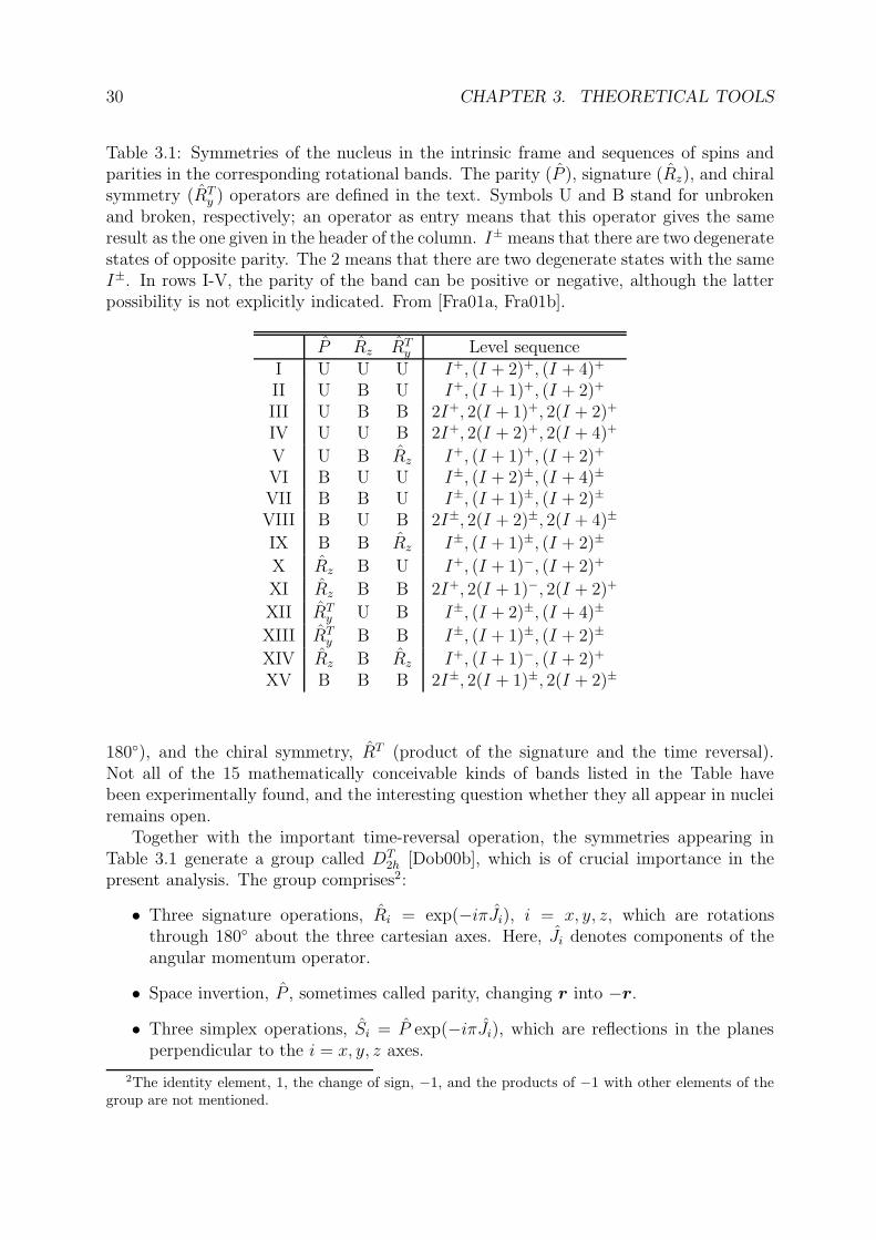
Table 3.1: Symmetries of the nucleus in the intrinsic frame and sequences of spins andparities in the corresponding rotational bands. The parity (P ), signature (Rz), and chiralsymmetry (RT
y ) operators are defined in the text. Symbols U and B stand for unbrokenand broken, respectively; an operator as entry means that this operator gives the sameresult as the one given in the header of the column. I± means that there are two degeneratestates of opposite parity. The 2 means that there are two degenerate states with the sameI±. In rows I-V, the parity of the band can be positive or negative, although the latterpossibility is not explicitly indicated. From [Fra01a, Fra01b].
P Rz RTy Level sequence
I U U U I+, (I + 2)+, (I + 4)+
II U B U I+, (I + 1)+, (I + 2)+
III U B B 2I+, 2(I + 1)+, 2(I + 2)+
IV U U B 2I+, 2(I + 2)+, 2(I + 4)+
V U B Rz I+, (I + 1)+, (I + 2)+
VI B U U I±, (I + 2)±, (I + 4)±
VII B B U I±, (I + 1)±, (I + 2)±
VIII B U B 2I±, 2(I + 2)±, 2(I + 4)±
IX B B Rz I±, (I + 1)±, (I + 2)±
X Rz B U I+, (I + 1)−, (I + 2)+
XI Rz B B 2I+, 2(I + 1)−, 2(I + 2)+
XII RTy U B I±, (I + 2)±, (I + 4)±
XIII RTy B B I±, (I + 1)±, (I + 2)±
XIV Rz B Rz I+, (I + 1)−, (I + 2)+
XV B B B 2I±, 2(I + 1)±, 2(I + 2)±
180), and the chiral symmetry, RT (product of the signature and the time reversal).Not all of the 15 mathematically conceivable kinds of bands listed in the Table havebeen experimentally found, and the interesting question whether they all appear in nucleiremains open.
Together with the important time-reversal operation, the symmetries appearing inTable 3.1 generate a group called DT
2h [Dob00b], which is of crucial importance in thepresent analysis. The group comprises2:
• Three signature operations, Ri = exp(−iπJi), i = x, y, z, which are rotationsthrough 180 about the three cartesian axes. Here, Ji denotes components of theangular momentum operator.
• Space invertion, P , sometimes called parity, changing r into −r.
• Three simplex operations, Si = P exp(−iπJi), which are reflections in the planesperpendicular to the i = x, y, z axes.
2The identity element, 1, the change of sign, −1, and the products of −1 with other elements of thegroup are not mentioned.
3.3. TILTED-AXIS CRANKING 31
• Antilinear time-reversal operator, T = exp(−iπsy)K, where sy is the y component
of the total intrinsic spin operator, and K is the complex conjugation in the spacerepresentation.
• T -signatures, RTi = T Ri, T-parity, P T = T P , and T -simplexes, ST
i = T Si, wherei = x, y, z.
The T -signatures are the chiral operators discussed in Section 2.2.When enumerating the DT
2h symmetries it is necessary to introduce names of the threecartesian axes. But obviously, the question in the mean-field calculations is not, e.g.,whether the signature with respect to some particular a priori given axis is broken or not.One says that the signature is broken uniquely if there is no axis i such that Ri is thesymmetry of the density. Otherwise, the signature is not broken. The same pertains to thesimplex, T -signature, and T -simplex symmetries. In the following, the terms broken andunbroken are always understood in this sense, when referring to the signature, simplex,T -signature, and T -simplex symmetries, unless a particular axis is specified.
3.3 Tilted-Axis Cranking
To obtain HF solutions describing states with higher angular momentum, particularly thelevels of a rotational band, one usually imposes a linear constraint on the total angularmomentum, and minimizes the mean value of the quantity called Routhian,
H ′ = H − ωJ , (3.10)
where the Lagrange multiplier ω is called rotational frequency, and J is the angular-momentum operator. This approach is called cranking approximation. Since H is rota-tionally invariant, the solutions obtained for the same length, but different directions ofω differ only by their orientation in space. Therefore, only the length, ω, has a physicalmeaning. The Kerman-Onishi theorem [Ker81a] states that, at the minimum, the totalangular momentum vector, J = 〈J〉, is parallel to ω. Indeed, this configuration obviouslyminimizes the mean value of the cranking term, −ωJ , while H is rotationally invariant.It comes from the variation of the many-body Routhian, H ′, that in the cranking modelthe s.p. Hamiltonian, h, is replaced by the s.p. Routhian,
h′ = h− ωJ , (3.11)
both in the HF equations (3.6) and in the theorem of self-consistent symmetries (3.9).If a given symmetry is not broken in a mean-field solution, expectation values of observ-
ables represented by operators odd under this symmetry vanish. Here, we are interestedin properties of the DT
2h symmetries with respect to the mean angular momentum vectorand electric quadrupole moment of the mass distribution, because they will play a fun-damental role in the search for broken signature and chiral symmetries. These propertiescan be summarized as (see [Dob00b] for a detailed derivation):
• If the time reversal, T , is not broken, all components of the angular momentumvanish, while the quadrupole moments are not affected.

32 CHAPTER 3. THEORETICAL TOOLS
• Unbroken parity, P , does not constrain neither the angular momentum nor thequadrupole moments.
• If Ri or Si is unbroken, the angular momentum can have a non-zero component onlyon the i-th axis, which in turn is a principal axis of the quadrupole tensor.
• If RTi or ST
i is unbroken, the axis i is a principal axis of the quadrupole tensor, whilethe angular-momentum vector is confined to the plane perpendicular to that axis.
These conclusions are valid, of course, for any arbitrarily oriented axis i, not only the x,y, z axes of some particular frame. It follows from the third bullet that if the angularmomentum has non-zero components on at least two principal axes of the quadrupoletensor, then there does not exist any axis i such that Ri or Si be an unbroken symmetry.The last point tells us that if the angular momentum has non-zero components on all thethree principal axes of the quadrupole tensor, then there is no such axis i that RT
i or STi
be unbroken.It is clear from the above properties of the DT
2h symmetries that whenever there existan axis i such that either Ri, Si, RT
i , or STi is an unbroken symmetry, then i is a principal
axis of the quadrupole tensor. So, only the principal axes and planes of this tensorare candidates to being symmetry axes and symmetry planes. It is, therefore, useful toconsider the intrinsic frame of reference, defined by the principal axes of the quadrupolemoment. To denote the axes of the intrinsic frame, the symbols s, m, l, are used, in viewof the short, medium and long axes of a triaxially deformed shape. Let us also introducethe program frame, which is defined by the axes used for solving the mean-field equations,e.g., in a computer code3. They are denoted as x, y, z. In general, the axes of the twoframes do not coincide.
If one wants to check by using the mean-field methods whether a given symmetryis spontaneously broken or not in the considered system, one looks for the minimum ofthe Routhian among trial solutions both breaking and not breaking the symmetry inquestion. Then one checks, to which of those two categories the minimum belongs. Theseare the symmetry-unrestricted calculations. One can also impose a given symmetry, whichamounts to searching for the Routhian minimum only among solutions that do not breakthat symmetry. When performing calculations with imposed DT
2h symmetries one can,without loss of generality, impose the symmetries associated with the axes of the programframe, e.g., Rx, which is technically much simpler. In fact, imposing either Ri, Si, RT
i orST
i , where i = x, y, z, causes that one of the intrinsic axes coincides with the program i-thaxis. In the following, the term imposed always has this meaning.
If some symmetries are imposed in the calculations, notably the cranking term, −ωJ ,must conform to them. This means that all the above restrictions concerning the meanangular momentum, J , equally touch the cranking frequency, ω. For example, solutionsinvariant under the time reversal may only result if no cranking is applied. These remarksallow us to introduce the following widely used classification of calculations with imposedsymmetries. Whenever a signature Ri or simplex Si symmetry is imposed, one can talk
3It would be unfortunate to call it laboratory frame, because in the common interpretation of thecranking model one would say that the program frame rotates in the laboratory system. The programand intrinsic frames do not move with respect to each other, they differ only by the orientation of theiraxes.
3.3. TILTED-AXIS CRANKING 33
about one-dimensional cranking, because the applied rotational frequency, ω, togetherwith all resulting (single-particle (s.p.) and total) angular momenta vectors, point alongthe unique, i-th axis. A name Principal-Axis Cranking (PAC) is also adopted, becausethe i-th axis is then a principal axis of the mass distribution (its quadrupole moment).In PAC calculations, the Kerman-Onishi condition (J ‖ ω) is satisfied identically. Inthe Tilted-Axis Cranking (TAC), all signature and simplex symmetries are broken, andtherefore the frequency, ω, and the mean angular momentum, J , vectors can becometilted with respect to the principal axes. If either a T -signature or T -simplex is stillimposed, these vectors remain in a single plain, and hence the name of planar or two-dimensional cranking (2D) is used. If not, ω and the resulting angular momentum, J ,can take any direction, and one talks about three-dimensional cranking (3D). In both the2D and 3D cases, still the parity can be either broken or not.
To solve the HF equations, one often uses the iterative method [Rin00a]. It followsfrom the theorem of self-consistent symmetries (see Section 3.1) that if a symmetry is notbroken in a certain iteration, it will remain so in all subsequent ones, and consequentlyin the final result. Therefore, to impose a symmetry it is enough to start the iterationsfrom an h even under this symmetry and also to apply the cranking frequency ω in aproper direction, as discussed above4. To render the calculations symmetry-unrestricted,either the initial h or the cranking term must violate the considered symmetry. If thesymmetry is not dynamically broken in the physical solution, it will recover in the courseof the iterations. In the present calculations, a DT
2h-symmetric Nilsson [Nil55a] potential
is always used as the first approximation to h, unless the iterations are restarted fromsome previously obtained solution. Therefore, the DT
2h symmetries can be broken onlyby the cranking term. If one wants to perform symmetry-unrestricted calculations fora non-rotating state, one may nevertheless apply a small cranking frequency in the firstiteration, only to break the DT
2h symmetries, and then continue with no cranking.
To relate the discussion to the magnetic and chiral rotation, after having performeda symmetry-unrestricted calculation one should verify whether the signature or chiralsymmetry is broken by considering the mean angular momentum vector in the intrinsicframe. If it has non-zero components on more than one intrinsic axis, then the signaturesymmetry is broken. If all three components are non-zero, also the chiral symmetryis broken. However, to make one sure that these symmetries are unbroken is not sostraightforward, because there may a priori exist other factors violating them, differentthat the angular momentum coupling, e.g., exotic deformations. A detection of unbrokensymmetries based on the values of the variational parameters (e.g., elements of the densitymatrix) would be doable, but difficult. Another way is to perform a separate calculationimposing the symmetry in question and then to check, whether the results are equivalent,i.e., whether they differ at most by orientation in space. This can be verified by looking atthe total energy, contributions thereto from the different terms of the Skyrme functional,density integrals, various observables, and s.p. energies.
A phenomenological approximation to the HF approach consists in replacing Γ witha model potential, like the Nilsson [Nil55a] or Woods-Saxon [Woo54a] one, which de-pends on several parameters, mainly multipole deformations, αλµ, of the nuclear surface.
4It is still possible that an initially unbroken symmetry breaks due to numerical noise. To avoid such anoise, in practical calculations the terms of h′ odd under the considered symmetry are simply disregarded.
34 CHAPTER 3. THEORETICAL TOOLS
Then, the expectation value of the Routhian h′ (corrected for the liquid drop energy viathe Strutinsky renormalization [Rin00a]) is minimized with respect to parameters of thepotential.
It is well understood that only the relative orientation of the angular momentum vectorand the intrinsic axes carries a physical information. Their position with respect to theprogram frame is meaningless and can be arbitrary. One can take advantage thereofin the phenomenological method, where the orientation of the mean potential is undercontrol via the variational parameters, like the multipole deformations αλµ of the nuclearsurface, and can be fixed so that the α2µ tensor be diagonal in the program frame simplyby setting α21 = Im α22 = 0. With this condition satisfied, the intrinsic frame coincideswith the program frame, facilitating many computational details. The minimization ofthe expectation value of the Routhian h′ at a given magnitude of ω is then performed byvarying the direction of ω and all αλµ except α21 and Im α22. The position of ω withrespect to the coinciding intrinsic and program frames is often described in the sphericalcoordinates, ϑ, ϕ, called tilt angles. It is in fact this procedure that is usually understoodunder the term TAC and that has been described many times in the literature, see e.g.the seminal papers by Frauendorf et al. [Fra91a, Fra92a, Fra93a, Fra97c, Fra00a] and[Dim00b].
In the HF method, however, the Euler angles defining the orientation of the intrinsicaxes are not free variational parameters, but complicated functions of the densities, thatchange from one iteration to another according to the HF recipe. Thus, the orientationcannot be easily controlled. The only feasible way to keep the nucleus in the axes of theprogram frame is by imposing dynamical constraints on the off-diagonal components ofthe quadrupole tensor and requiring that they vanish. Then, one can vary the crankingfrequency vector like in the phenomenological approach. It is actually the only way toproceed if the energy dependence on the tilt angles, ϑ, ϕ, is sought. It has been checked,however, that multipole constraints strong enough to confine the nucleus may easily leadto divergenciesm, at least in the present calculations. If only the minimum is of interest,a more natural and faster way is to fix the rotational frequency vector with respect to theprogram frame and let the mean potential reorient and conform to it self-consistently inthe course of the iterations. It is but this procedure that corresponds to the minimizationof the given Routhian (3.10). The direction of the rotational frequency vector in theprogram frame no more plays any role, while the solution now does become tilted withrespect to that frame. This method has been adopted in the present work.
Some quantities, like mean angular momenta and multipole moments, carry a clearinformation only when expressed in the intrinsic frame of the nucleus. But they are firstcalculated in the program frame. Since the two no more coincide, it is necessary to find theprincipal axes of the nuclear shape by diagonalization of the electric quadrupole tensorand to transform the considered quantities into the corresponding frame by use of theWigner matrices.
To examine deformed nuclei one usually choses deformed bases. However, deformationof the basis improves the description only if it suites the shape of the nucleus; otherwiseit may spoil the result. For instance, deformation of the Harmonic-Oscillator (HO) basisamounts to stretching the cartesian coordinates associated with the axes of the programframe, and to taking different numbers of quanta in each direction. This is not appropriate
3.4. THE HF TIME-ODD COUPLING CONSTANTS 35
for representing the TAC solutions, whose principal axes are arbitrarily tilted with respectto the program frame. A deformed basis would drive such a solution like a force toa certain orientation different from the self-consistent one, determined by the directionof the cranking vector. In particular, the Kerman-Onishi condition would be violated.Therefore, in self-consistent TAC calculations, the s.p. space spanned by the basis shouldbe rotationally invariant. It means that the basis should have the three characteristicfrequencies equal and comprise only entire HO shells. To obtain a reasonable descriptionfor deformed nuclei, the only way is to use large bases.
It follows from the theorem of self-consistent symmetries that the s.p. Routhian andthe density matrix are invariant under the same symmetry operations; see Section 3.1.However, one should be aware of one exception to that rule, that concerns the time-reversalsymmetry in case the time-odd terms of the mean field are artificially set to zero in thecalculations. This simplification is always the case in the phenomenological mean-fieldapproach, where time-odd terms simply do not appear in the model potential. With thetime-odd fields cut off (and with no cranking), the Routhian is explicitly time-even, whilethe density will still acquire time-odd components whenever there is an unpaired particle;see Appendix A. The spectrum of the time-even Routhian exhibits the two-fold Kramersdegeneracy, and the state of the unpaired particle can be any unitary combination of thestates in the Kramers pair; the physicist must take the decision. The main point of thisdiscussion is that this freedom of choice influences the time-odd densities, while the time-even ones remain undisturbed. This lemma is proven in Appendix A. Together with thetime-odd densities, also the time-odd observables, notably the mean angular momentum,depend on that choice. The time-even quantities, like the quadrupole moments, areuniquely determined, because they depend only on time-even densities. These conclusionsare valid for both the phenomenological and the self-consistent implementation of themean-field method. However, in the self-consistent approach, in each iteration there isa feedback from the density to the mean field. One may doubt, therefore, whether thechoice of state for the unpaired particle alters the generated mean field. This is not thecase, because the time-even fields originate only from the time-even density, which arenot disturbed, while the time-odd fields are suppressed.
3.4 The HF time-odd coupling constants
One important point in the investigations of the magnetic and chiral rotation is to examinethe role of various time-odd observables, like current and magnetic-moment distributions.Their impact on the results is governed by the time-odd coupling constants of the HFenergy functional. After introducing necessary definitions of the local densities, energyfunctional, mean fields, and local gauge invariance, this Section explains how the valuesof the time-odd coupling constants are set in the present calculations.
In the HF approximation, the total energy is, in general, a functional of the non-localone-body density,
ρα(rσ, r′σ′) = 〈Ψ|a+r′σ′αarσα|Ψ〉 , (3.12)
where |Ψ〉 is the many-body wavefunction, r and σ are the position and spin variables,and α = n, p for neutrons and protons, respectively. The density ρα(rσ, r′σ′) can be
36 CHAPTER 3. THEORETICAL TOOLS
written as a sum of the scalar, ρα(r, r′), and vector, sα(r, r′), terms,
ρα(r, r′) =∑
σ
ρα(rσ, r′σ′) , sα(r, r′) =∑
σσ′
ρα(rσ, r′σ′)σσ′σ, (3.13)
asρα(rσ, r′σ′) = 1
2ρα(r, r′)δσσ′ + 1
2sα(r, r′) · σσσ′ . (3.14)
The HF equations are usually solved within the Local-Density Approximation (LDA), inwhich the total energy depends only on local (r = r′) densities, and on their derivatives atr = r′ up to the second order. One has to consider the following real nucleonic densities[Eng75a]:
Particle: ρα(r) = ρα(r, r) ,Spin: sα(r) = sα(r, r) ,Kinetic: τα(r) = [∇ ·∇′ρα(r, r′)]
r=r′ ,
Vector kinetic: T α(r) = [∇ ·∇′sα(r, r′)]r=r
′ ,Momentum: jα(r) = 1
2i[(∇−∇
′)ρα(r, r′)]r=r
′ ,Spin-current: Jµν,α(r) = 1
2i
[
(∇µ −∇′µ)sν,α(r, r′)
]
r=r′ ,
(3.15)
of which ρα, τα, and←→J α = Jµν,α are time-even, and sα, T α, and jα are time-odd. For
each of the local densities, one defines the isoscalar and isovector density, e.g.,
ρ0 = ρn + ρp ρ1 = ρn − ρp (3.16)
The isoscalar and isovector terms are denoted by subscript t = 0, 1, respectively.The interaction part of the HF LDA energy functional can be expressed as a space
integral,
E =∑
t
∫
d3r(
Hevent +Hodd
t
)
, (3.17)
of energy densities, Hevent and Hodd
t , which depend on the time-even and time-odd nucle-onic densities, respectively. They are defined as
Hevent (r) = Cρ
t ρ2t + C∆ρ
t ρt∆ρt + Cτt ρtτt + CJ
t
←→J 2
t + C∇Jt ρt∇ · J t ,
Hoddt (r) = Cs
t s2t + C∆s
t st ·∆st + CTt st · T t + Cj
t j2t + C∇j
t st · (∇× jt) ,(3.18)
where the square of the tensor density is defined as←→J 2
t =∑
µν J2µν,t, and its vector part,
J t, is defined as Jλ,t =∑
µν ελµνJµν,t. The coupling constants Ct appearing in Hevent and
Hoddt are conventionally called time-even and time-odd, respectively. They are functions
of the parameters of the Skyrme force [Dob95a], and may depend on density if the force isdensity-dependent. Note, however, that in the spirit of the Density-Functional Theory theenergy functional does not need to come from any interaction, and the coupling constantsCt play the role of fundamental parameters.
Upon variation of the interaction energy, E , with respect to local densities, one obtainsthe neutron and proton Skyrme-HF s.p. mean potentials (see Section 3.1),
Γn = Γeven0 + Γodd
0 + Γeven1 + Γodd
1 Γp = Γeven0 + Γodd
0 − Γeven1 − Γodd
1 , (3.19)
3.4. THE HF TIME-ODD COUPLING CONSTANTS 37
where the time-even and time-odd fields, Γevent and Γodd
t , read
Γevent = −∇ · [Mt∇] + Ut + 1
2i
(←→∇σ · ←→B t +←→B t ·
←→∇σ)
,
Γoddt = −∇ · [(σ ·Ct) ∇] + σ ·Σt + 1
2i(∇ · I t + It ·∇) .
(3.20)
They depend on the nucleonic densities through the potential functions,
Ut(r) = 2Cρt ρt + 2C∆ρ
t ∆ρt + Cτt τt + C∇J
t ∇ · J t + U ′t ,
Σt(r) = 2Cst st + 2C∆s
t ∆st + CTt T t + C∇j
t ∇× jt ,Mt(r) = Cτ
t ρt ,Ct(r) = CT
t st ,←→B t(r) = 2CJ
t
←→J t − C∇J
t
←→∇ ρt ,
I t(r) = 2Cjt jt + C∇j
t ∇× st .
(3.21)
The tensor gradient operators in (3.20) and (3.21) are defined as (←→∇σ)µν = ∇µσν and
∇µν =∑
λ εµνλ∇λ. The term U ′t represents the rearrangement terms resulting from the
density dependence of the coupling constants, Ct. In standard parametrizations of theSkyrme interaction, which are used in the present work, only Cρ
t and Cst depend on the
isoscalar particle density, ρ0, and then
U ′0(r) =
∑
t′
(
∂Cρt′
∂ρ0ρ2
t′ +∂Cs
t′
∂ρ0s2
t′
)
U ′1(r) = 0 . (3.22)
If the energy functional is derived from the Skyrme interaction, there are uniquerelations between the time-even and time-odd coupling constants, Ct. In particular,
Cjt = −Cτ
t , CJt = −CT
t , C∇jt = +C∇J
t . (3.23)
However, it turns out [Dob95a] that the three relations (3.23) have a deeper sense, namely,they are necessary and sufficient conditions for the invariance of the energy functionalunder a local gauge transformation of the A-body wave-function, |Ψ〉,
|Ψ′〉 = exp
(
i
A∑
j=1
φ(rj)
)
|Ψ〉 , (3.24)
where φ(r) is an arbitrary real function of position. In particular, for φ = p · r/h, thegauge transformation (3.24) corresponds to a Galilean boost with velocity v = p/m,where m is the particle mass.
In the present calculations, the SLy4 [Cha97a] and SkM* [Bar82a] parametrizations ofthe Skyrme force were used. Like in the original fits, the time-even coupling constant CJ
t
and the time-odd constant CTt were always set to zero. This does not hamper the local
gauge invariance. Apart from CJt , all other time-even coupling constants were taken as
they come from the parameters of the Skyrme force. To examine the role of the time-odddensities and fields, attempts were undertaken to obtain each solution with three sets ofvalues of the time-odd coupling constants. In each case, values of selected constants weretaken as they come from the Skyrme force, while those of the remaining ones were set to
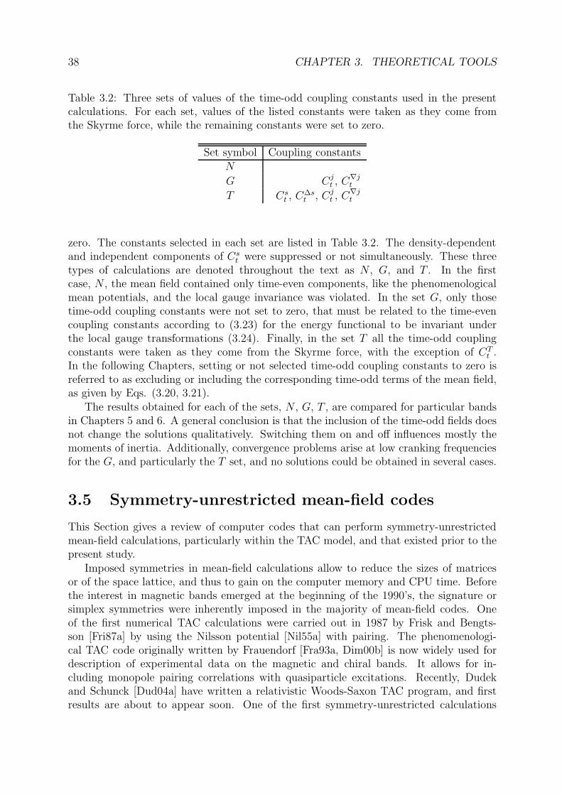
38 CHAPTER 3. THEORETICAL TOOLS
Table 3.2: Three sets of values of the time-odd coupling constants used in the presentcalculations. For each set, values of the listed constants were taken as they come fromthe Skyrme force, while the remaining constants were set to zero.
Set symbol Coupling constantsN
G Cjt , C∇j
t
T Cst , C∆s
t , Cjt , C∇j
t
zero. The constants selected in each set are listed in Table 3.2. The density-dependentand independent components of Cs
t were suppressed or not simultaneously. These threetypes of calculations are denoted throughout the text as N , G, and T . In the firstcase, N , the mean field contained only time-even components, like the phenomenologicalmean potentials, and the local gauge invariance was violated. In the set G, only thosetime-odd coupling constants were not set to zero, that must be related to the time-evencoupling constants according to (3.23) for the energy functional to be invariant underthe local gauge transformations (3.24). Finally, in the set T all the time-odd couplingconstants were taken as they come from the Skyrme force, with the exception of CT
t .In the following Chapters, setting or not selected time-odd coupling constants to zero isreferred to as excluding or including the corresponding time-odd terms of the mean field,as given by Eqs. (3.20, 3.21).
The results obtained for each of the sets, N , G, T , are compared for particular bandsin Chapters 5 and 6. A general conclusion is that the inclusion of the time-odd fields doesnot change the solutions qualitatively. Switching them on and off influences mostly themoments of inertia. Additionally, convergence problems arise at low cranking frequenciesfor the G, and particularly the T set, and no solutions could be obtained in several cases.
3.5 Symmetry-unrestricted mean-field codes
This Section gives a review of computer codes that can perform symmetry-unrestrictedmean-field calculations, particularly within the TAC model, and that existed prior to thepresent study.
Imposed symmetries in mean-field calculations allow to reduce the sizes of matricesor of the space lattice, and thus to gain on the computer memory and CPU time. Beforethe interest in magnetic bands emerged at the beginning of the 1990’s, the signature orsimplex symmetries were inherently imposed in the majority of mean-field codes. Oneof the first numerical TAC calculations were carried out in 1987 by Frisk and Bengts-son [Fri87a] by using the Nilsson potential [Nil55a] with pairing. The phenomenologi-cal TAC code originally written by Frauendorf [Fra93a, Dim00b] is now widely used fordescription of experimental data on the magnetic and chiral bands. It allows for in-cluding monopole pairing correlations with quasiparticle excitations. Recently, Dudekand Schunck [Dud04a] have written a relativistic Woods-Saxon TAC program, and firstresults are about to appear soon. One of the first symmetry-unrestricted calculations
3.6. THE PROGRAM hfodd (V2.05C) 39
within realistic self-consistent methods were performed in 1991 by Umar et al. [Uma91a].Without cranking and pairing, they solved the Skyrme-HF equations in the space rep-resentation, by using the Spline Collocation Method. About the year 2000, Yamagamiand Matsuyanagi developed a symmetry-unrestricted Skyrme-HF program working on aCartesian mesh with the imaginary-time method [Yam00a, Yam01a]. They include ei-ther only cranking or only pairing with the density-dependent delta force and withoutquasiparticle excitations. Calculations of Madokoro et al. for a magnetic band in 84Rb[Mad00a] were done in 2000 by use of a Relativistic Mean Field TAC code imposing onlythe parity, working in the harmonic-oscillator basis and not including pairing. For thepurpose of the present work, the author developed a Skyrme-HF TAC program, hfodd
version (v2.05c), that works in the harmonic-oscillator basis and allows for breaking of allthe DT
2h symmetries. Currently, the pair correlations cannot be taken into account in theTAC mode. This program is described in the next Section.
3.6 The program hfodd (v2.05c)
In order to perform self-consistent calculations for the magnetic and chiral rotation, theauthor of this work developed a Skyrme-HF computer code, hfodd version (v2.05c). Inthe previous versions, (v1.60r) and (v1.75r) [Dob00a], the simplex symmetry was imposed,thus not allowing for TAC calculations. Removing this restriction was the principal im-provement introduced during the present work, and led to the version (v2.05c), whichwas used for obtaining results presented here. A brushed-up version, (v2.08i), was pub-lished in [Dob04a]. This Section gives an overview of the program’s main features, withparticular emphasis on those that have been introduced for the purpose of the presentinvestigations.
The code hfodd solves the nuclear HF equations for the Skyrme effective interactionby using the iterative method. The s.p. wavefunctions are expanded onto the deformedCartesian Harmonic-Oscillator (HO) basis. From the s.p. wavefunctions, the HF localdensities (3.15), and then the mean potentials (3.20) are calculated on a Cartesian mesh.By using the Gauss-Hermite quadrature, matrix elements of those potentials between theHO states are calculated. The matrix of the s.p. Hamiltonian, obtained in this way, isthen diagonalized, to find the s.p. wavefunctions in the next iteration. The Nilsson po-tential [Nil55a] is implemented as a starting point. All densities (3.15) appearing in theSkyrme functional are calculated, and all time-even and time-odd fields (3.20) are takeninto account. Several parametrizations of the force are available and can be modified.The generalized spin-orbit terms [Rei95a] can be included in the Skyrme functional. Ap-propriate time-odd coupling constants of the energy functional can be determined eitherfrom the Skyrme force or from the Landau parameters [Ben02a]. For the center-of-massmotion, either the standard one-body correction before variation or a two-body correc-tion after variation can be used. Apart from such basic quantities like s.p. and totalenergies, the code calculates the angular momentum vectors, electric, magnetic, and sur-face multipole moments, mean-square radii and Bohr deformation parameters. Linear andquadratic constraints on spin as well as quadratic constraints on the electric and surfacemoments are implemented. With the simplex imposed as an unbroken symmetry, theprogram can also work in the HFB mode, with either the fixed-gap or density-dependent
40 CHAPTER 3. THEORETICAL TOOLS
delta pairing. The Fermi level is found automatically by using the equivalent-spectrummethod [Dob84a]. The quasi-particle blocking is not yet programmed.
The user can choose the pattern of imposed symmetries by independently imposingor not the Sy, Ry, P , T , ST
x , STy , and ST
z symmetries. Keeping in mind that the unbrokensymmetries must form a group, 34 combinations listed in Table 3.3 are permitted. Someof them differ only by an exchange of the Cartesian axes associated with the signatureand simplex symmetries, and are thus physically equivalent. Altogether, 19 out of the 28non-equivalent subgroups5 of DT
2h can be selected as imposed symmetries. Imposing themissing 9 subgroups can easily be implemented provided there is a physics motivation tostudy such new cases. When either of the three symmetries, Sy, Ry, or P is imposed,the s.p. Routhian acquires a specific block-diagonal form, and diagonalization of smallermatrices results in a faster execution time. In version (v2.08i), this is implemented forSy and/or P imposed, but in case Ry alone is imposed it is not implemented yet. Thethree T -simplexes and the time reversal cannot be used in a similar way, because theyare represented by anti-linear operators. However, when the time reversal and simplexor signature are imposed, the Kramers degeneracy allows for diagonalization of matricesonly in one simplex or signature, which reduces the numerical effort by half. The codestores the Skyrme local densities on a Cartesian mesh, and takes advantage of imposedsymmetries, both represented by linear and anti-linear operators, to reduce the numberof lattice points on which the densities are calculated.
Arbitrary s.p. configurations can be required in the code hfodd, and the way ofselecting them is related to the pattern of imposed symmetries. If P and Ry are imposed,then the s.p. states are divided into four groups characterized by the parity and signatureeigenvalues. Those groups are referred to as parity-signature blocks. The code does notput the particles just on the energetically lowest s.p. states, but the user must specify thenumbers of particles in each block separately. Then, in each block, the lowest levels areoccupied, which gives the reference configuration, from which the particle-hole excitationare counted afterwards. The same is implemented for imposing either of P , Ry, or Sy
alone, only that in these cases there are two blocks instead of four. They are called parity,signature, and simplex blocks, respectively. If no symmetries are imposed, obviouslythere is only one block. The three T -simplexes and the time reversal do not play anyrole in this mechanism, because anti-linear operators do not provide quantum numbers.In the following, the parity-signature reference configuration is specified as (n++, n+−,n−+, n−−), where, e.g., n+− is the number of occupied states of parity +1 and signature−i, etc. Similarly, the parity, signature, and simplex reference configurations are givenas (n+, n−). States in parity-signature blocks are denoted as, e.g., 18– +, which refersto the eighteenth state of negative parity and positive signature, counting from one inenergetical order. Sometimes, a pair of states, like 18– + and 18– –, is denoted as 18–±.The notation for the parity, signature, and simplex blocks is similar, e.g., 28 –. Particle-hole excitations are defined by selecting from which state in which symmetry block aparticle is removed and onto which state in which block it is put. This is denoted as,e.g., (18– +→ 19– +) for the parity-signature case and, e.g., (28 –→ 29 –) for the parity,signature, or simplex imposed. The use of symmetry blocks makes it easier to follow agiven configuration diabatically, because crossings of levels belonging to different blocks
5Including the trivial subgroups.
3.6. THE PROGRAM hfodd (V2.05C) 41
Table 3.3: Complete list of imposed (I) or non-imposed (N) symmetries allowed in thecode hfodd version (v2.08i). The first column enumerates all the possible symmetrypatterns, while the second column enumerates non-equivalent subgroups (see text).
Number Symmetries Conserved group
Sy Ry P T STy ST
x STz
1 1 I I I I I I I Rxyz P Sxyz T RTxyz P T ST
xyz
2 2 I I I I I N N Ry P Sy T RTy P T ST
y
3 3 I I I N N I I Ry P Sy RTzx ST
zx
4 4 I I I N N N N Ry P Sy
5 5 I N N I I I N Rz Sxy T RTz ST
xy
6 5 I N N I I N I Rx Syz T RTx ST
yz
7 6 I N N I I N N Sy T STy
8 7 I N N N N I N Sy RTz ST
x
9 7 I N N N N N I Sy RTx ST
z
10 8 I N N N N N N Sy
11 5 N I N I N I I Ry Szx T RTy ST
zx
12 9 N I N I N N N Ry T RTy
13 10 N I N N I I I Rxyz P T STxyz
14 11 N I N N I N N Ry P T STy
15 12 N I N N N I I Ry STzx
16 13 N I N N N N N Ry
17 2 N N I I N I N Rx P Sx T RTx P T ST
x
18 2 N N I I N N I Rz P Sz T RTz P T ST
z
19 14 N N I I N N N P T P T
20 3 N N I N I I N Rz P Sz RTxy ST
xy
21 3 N N I N I N I Rx P Sx RTyz ST
yz
22 15 N N I N I N N P RTy ST
y
23 15 N N I N N I N P RTx ST
x
24 15 N N I N N N I P RTz ST
z
25 16 N N I N N N N P
26 6 N N N I N I N Sx T STx
27 6 N N N I N N I Sz T STz
28 17 N N N I N N N T
29 12 N N N N I I N Rz STxy
30 12 N N N N I N I Rx STyz
31 18 N N N N I N N STy
32 18 N N N N N I N STx
33 18 N N N N N N I STz
34 19 N N N N N N N
42 CHAPTER 3. THEORETICAL TOOLS
do not cause any confusion as to which of them should be occupied. If two levels from thesame block are about to cross near the Fermi surface, the user may require that a statewith a lower/higher value of a certain s.p. observable be occupied. In the present context,such diabatic blocking concerns primarily the projection of the s.p. angular momentumon the cranking frequency vector.
The code allows for TAC calculations, and there are no restrictions on the directionof the angular frequency vector, except for those following from the imposed symmetries.According to the Kerman-Onishi theorem [Ker81a], in TAC calculations all self-consistentsolutions have their spin and cranking frequency vectors, J and ω, parallel. In practice,J approaches ω very slowly in the course of the iterations, and up to several thousandsof iterations are necessary to obtain a converged result. To avoid this inconvenience, aquadratic constraint on the vector product, ω×J , has been introduced, constraining thatquantity to zero. However, this does not speed up the convergence significantly, and mayeasily lead to divergencies. In version (v2.08i), a different prescription was implemented,which is much more stable and substantially reduces the required number of iterations.Namely, in each iteration, the rotational frequency vector is explicitly reset to be parallelto the current total angular momentum vector, while its length, ω, is kept unchanged.Since ω is not constant in this method, it does not correspond to minimization of any apriori given Routhian. However, it is the Routhian with the last direction of ω that willhave been minimized once the converged solution is found. This method was inventedafter the completion of the present calculations, and was not yet implemented in version(v2.05c). This is the only difference between the two versions that matters for the presentstudy.
Some quantities, like the multipole moments, only carry a clear information if cal-culated with respect to the center of mass. As far as the symmetry patterns used inthe code (see Table 3.3) are concerned, if neither the parity nor T -parity is imposed,the center-of-mass of the solution may move away from the origin of the program frame.The code then finds its position and recalculates the quantities in question in the center-of-mass frame. It is also useful to compute the spin vectors and all types of multipolemoments in the intrinsic frame of the nucleus, defined by the principal axes of the electricquadrupole tensor. Unless any two of the simplex symmetries, Sx, Sy, Sz, ST
x , STy , ST
z ,are imposed, the principal axes may become tilted with respect to the Cartesian axes ofthe program frame; see Section 3.3. The code then finds the directions of the principalaxes by diagonalization of the quadrupole tensor, and transforms all necessary quantitiesto the intrinsic system of reference. If the parity is not imposed, the solution may acquirenon-zero linear momentum. The code computes its value and corrects the mean angularmomenta for that translational motion.
Chapter 4
Properties of the h11/2 valencenucleons
Behavior of the shears and chiral bands is, to a big extent, determined by the rotationalproperties of the valence high-j particles and holes. In the cases studied here, we areprimarily interested in properties of the h11/2 orbital. In this Chapter, some generalproperties of the h11/2 states are analyzed, first within self-consistent one-dimensionalcranking method, and then analytically. It is demonstrated that those properties areaffected by the triaxial deformation and that the concerned valence nucleons are expectedto align their angular momenta rather stiffly along the principal axes of the triaxial shape.It is also argued that pairing correlations may soften those alignments.
4.1 Symmetries of the non-rotating solutions
In the following two Chapters, Hartree-Fock (HF) shears solutions in 142Gd and chiralsolutions in 130Cs, 132La, 134Pr, 136Pm are presented. Calculations were carried out withtwo Skyrme-force parametrizations, SLy4 [Cha97a] and SkM* [Bar82a], with and withoutthe HF time-odd fields included; see Section 3.4. Since there is no physical indicationfor the breaking of parity in either of the shears or chiral bands, this symmetry was im-posed in the calculations. For all considered nuclides, symmetry-unrestricted calculations(modulo the imposed parity) were performed to check, whether some other symmetriesare spontaneously broken in the non-rotating states. Whenever the time-odd fields wereabsent (either switched off or self-consistently zero in the ground state of the even-even142Gd), it was found that the mean field possessed the DT
2h symmetry. This was inferredfrom comparison of the symmetry-unrestrained results with those obtained with the DT
2h
symmetry imposed1, as described in Section 3.3.
1In hfodd, for configurations with unpaired nucleons, the DT2h symmetry can be imposed on the mean
field by imposing P , Sy, STx , ST
z , and switching the time-odd fields off.
43
44 CHAPTER 4. PROPERTIES OF THE H11/2 VALENCE NUCLEONS
4.2 Single-particle PAC Routhians for triaxial nuclei
All the HF solutions considered in the present work are triaxial, and this property deter-mines many of their features. It is instructive to examine their rotations about the threeprincipal axes first. This amounts to applying Principal-Axis Cranking (PAC), with bothparity and signature imposed. For non-rotating states with the time-odd terms absent,the mean field is anyway symmetric with respect to the whole DT
2h group, and imposingeither of the three signatures does not change it. Although the associated Slater determi-nants can be different for different signatures imposed, due to different signature stateschosen for unpaired particles, this does not affect the mean field; see Section 3.3 for de-tails. Thus, it is justified to say that three different rotations of the same triaxial objectare considered. With the time-odd fields present, the symmetry-unrestrained solutionsviolate all the three signatures. Therefore, imposing any of them necessarily leads to asubstantially different solution, and different for each of the signatures imposed. How-ever, the energies, deformations, and s.p. energies are very similar, and the effects fromthe time-odd fields are not so strong. In the code hfodd, it is technically most convenientto perform PAC about the y axis2. To examine rotation about each given intrinsic axis,the non-rotating solutions were first turned in space, by use of appropriate quadrupoleconstraints, so that the required principal axis coincide with the program y axis.
Sample self-consistent s.p. PAC Routhians for 130Cs, 132La, 134Pr, 136Pm, and 142Gdare collected in Appendix D. The s.p. levels are numbered so that, e.g., 14–+ denotes thefourteenth level of negative parity and positive signature; see Section 3.6. In non-rotatingsolutions, the s.p. levels originating from the spherical h11/2 orbital have numbers 14–±to 19–± (each level comprising two states of opposite signatures), for both protons andneutrons. This was checked in calculations with constraints on the quadrupole momentby the observation that the s.p. energies of the levels 14–± to 19–± converge to thesame value with decreasing β, and no crossings with other negative-parity levels occur3
in function of β. In the spherical case, the h11/2 s.p. levels unambiuously have numbers14–± to 19–± in all realistic potentials, because h11/2 is an intruder orbital, well separatedfrom all other negative-parity states.
For cranking about the short axis, the lowest sublevels of the h11/2 orbital (14–±) splitstrongly in function of ω, while the highest (19–±) do not. For the long axis, it is preciselythe opposite, while for the medium axis only the intermediate levels split. Routhians forcranking about the medium axis are given only in Figs. D.6 and D.7, for the sample caseof 132La. In fact, the intermediate h11/2 levels split for cranking about each of the threeaxes, but only weakly. Slopes of the PAC Routhians, e′, translate into the s.p. alignments,ji, on the i-th axis according to the well-known formula
ji = − de′
dωi
, (4.1)
which holds exactly for fixed mean potentials and approximately if the potential changeswith rotational frequency due to the HF self-consistency or TRS minimization. Therefore,
2Although PAC about the x and z axes is also implemented, conservation of the associated simplexor signature symmetries does not yield block-diagonal matrices in the basis used [Dob04a].
3With the exception of the triaxial minima in 134Pr and 136Pm; see Section 6.2.
4.3. DT2 -SYMMETRIC MEAN FIELD 45
the lowest h11/2 sublevels align their angular-momenta vectors on the short axis, andthe highest on the long one. The corresponding alignments are approximately equal to11/2 h. The intermediate states have non-zero alignments on all the three axes. Althoughthese results are based on PAC calculations, they are confirmed in the full Tilted-AxisCranking (TAC) results of Chapters 5 and 6. For the DT
2h-symmetric mean fields, thealignments obtained from one-dimensional cranking acquire a very specific meaning, whichis discussed in the next Section.
4.3 DT2 -symmetric mean field
In all the present HF solutions without the time-odd fields, as well as in virtually all phe-nomenological studies of the magnetic and chiral rotation, the mean-field Hamiltonian, h,is symmetric under the DT
2h group. In such a case, important properties of the s.p. statescan be inferred from pure symmetry considerations. Eigenstates of a DT
2h-symmetric po-tential exhibit the two-fold Kramers degeneracy, and this Section is focused on propertiesof a single Kramers pair. In fact, to obtain the results of this Section, it is enough toassume that h is symmetric with respect to DT
2 , a subgroup of DT2h which consists of the
time reversal, the three signature, and the three T -signature operations.A complete information about the matrix elements of the angular-momentum operator,
J , between the states of a Kramers pair, (|µ〉, |µ〉), is contained in the real alignmentvector, Jµ, and the complex decoupling vector, Dµ, of the state |µ〉,
Jµ = 〈µ|J |µ〉 , Dµ = 〈µ|J |µ〉 . (4.2)
The alignment and decoupling vectors, J µ, Dµ, of the state |µ〉 are related to Jµ and Dµ,by Eq. (B.2); see Appendix B. For any Hamiltonian, h, invariant under the DT
2 group, onecan choose the states of the considered Kramers pair as eigenstates of either of the threesignatures, Ri, where i = x, y, z. This results in three formally different pairs, (|µi〉, |µi〉),that correspond to just three different bases in the same two-dimensional eigenspace ofh. It is shown in Appendix B, that there are only three independent real parametersthat determine all components of the alignment and decoupling vectors associated withthe three examined pairs. These are the ”diagonal” components Jµx
x , Jµyy , Jµz
z , where thelower indices refer to the Cartesian components of J . One has
Jµx = (Jµx
x , 0, 0) , Dµx = (0, Jµy
y ,−iJµz
z ) , (4.3)
Jµy = (0, Jµy
y , 0) , Dµy = (−iJµx
x , 0, Jµz
z ) , (4.4)
Jµz = (0, 0, Jµz
z ) , Dµz = (Jµx
x ,−iJµy
y , 0) . (4.5)
Invariance of h under DT2 does not restrict the values of Jµx
x , Jµyy , Jµz
z . In the oftenconsidered case of axial symmetry, say with respect to the z axis,
(Jµx
x , Jµy
y , Jµz
z ) =
(Jµ⊥
⊥ , Jµ⊥
⊥ , Jµ‖
‖ ) for Jµ‖
‖ = 1/2
(0, 0, Jµ‖
‖ ) for Jµ‖
‖ = 3/2, 5/2, ...(4.6)
The component Jµ‖
‖ is quantized due to the axial symmetry, and the still arbitrary com-
ponent Jµ⊥
⊥ is usually called decoupling parameter; see Appendix B for details.
46 CHAPTER 4. PROPERTIES OF THE H11/2 VALENCE NUCLEONS
Suppose that the states in the considered Kramers pair have no coupling to other statesthrough the angular-momentum operator. Under this assumption, the 3D cranking for thispair becomes a two-dimensional diagonalization problem, that can be solved analytically.Of course, it concerns the non-selfconsistent cranking, where the Hamiltonian h in theRouthian h′ is fixed. For a degenerate Kramers pair, h reduces to its eigenvalue, e. Taking,e.g., the states |µz〉, |µz〉 as a basis one has, according to (4.5),
h′ = h− ωJ =
[
e 00 e
]
−[
ωzJµzz ωxJ
µxx − iωyJ
µyy
ωxJµxx + iωyJ
µyy −ωzJ
µzz
]
. (4.7)
For the eigenstates of h′, one obtains the following components of the mean angularmomentum vector, J ,
Ji = ± ωi(Jµi
i )2
(
ω2x(Jµx
x )2 + ω2y(J
µyy )2 + ω2
z(Jµzz )2
)1/2. (4.8)
They differ by sign for the two eigenstates. This dependence has a singularity at ω = 0,and is not linear in the general case. Consider the following two extreme situations. IfJµx
x = Jµyy = Jµz
z = g, then Ji = gωi/ω, and J always orients itself along ω, already forinfinitesimal ω. This can be called soft alignment. On the other hand, when only one ofthe parameters Jµx
x , Jµyy , Jµz
z is non-zero, say Jµj
j , then Ji = Jµj
j δij , and J is independentof ω (unless ω = 0). We call this stiff alignment on the j-th axis.
In axial nuclei, precisely one two-fold degenerate substate of each deformation-splitj-shell has J
µ‖
‖ = 1/2 and Jµ⊥
⊥ 6= 0, which represents the soft alignment. According
to Eq. (4.6), all other necessarily have a vanishing decoupling parameter, and are thusrigidly aligned with the symmetry axis. For prolate shapes, the lowest-energy substate hasJ
µ‖
‖ = 1/2, and is soft, while for oblate shapes it is the highest substate. In triaxial nuclei,
values of the parametrs Jµi
i , where i = s, m, l corresponds to the short, medium, and longprincipal axes, are equal to the alignments obtained from the one-dimensional crankingabout the three axes. Indeed, for cranking about the axis i, the s.p. states are eigenstatesof Ri. Taking into account the PAC results of the previous Section, one can see that forthe lowest h11/2 substates of a triaxial nucleus only Jµs
s is non-zero, while for the highestsubstates only Jµl
l does not vanish. These alignments are thus stiff. The Routhians ofthese states are not much curved, which confirms that their angular-momentum couplingto other states is rather weak. Note that there are no states with stiff alignment on themedium axis. The response to rotation of the middle h11/2 substates is soft, becauseall the three parameters, Jµs
s , Jµmm , Jµl
l , are non-zero, and complicated, because thesestates interact with one another, what can be seen from the strong bending of their PACRouthians.
Although the presented results come from a non-selfconsistent cranking (with fixed h),the full HF calculations in Chapters 5 and 6 show that at least the deformation does notchange much with rotational frequency, particularly for the chiral bands. Therefore, thenon-selfconsistent cranking should be a good approximation here. In both the magneticand chiral bands, the active high-j particles occupy the lowest substates of a given orbital,while the valence holes occupy the highest substates. The principal conclusion of the lasttwo Sections is, therefore, that those valence particles and holes align their individual
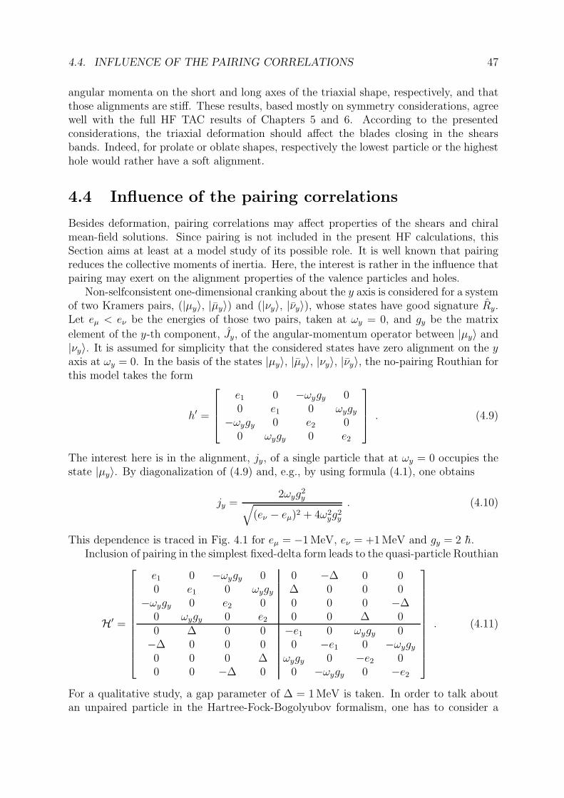
4.4. INFLUENCE OF THE PAIRING CORRELATIONS 47
angular momenta on the short and long axes of the triaxial shape, respectively, and thatthose alignments are stiff. These results, based mostly on symmetry considerations, agreewell with the full HF TAC results of Chapters 5 and 6. According to the presentedconsiderations, the triaxial deformation should affect the blades closing in the shearsbands. Indeed, for prolate or oblate shapes, respectively the lowest particle or the highesthole would rather have a soft alignment.
4.4 Influence of the pairing correlations
Besides deformation, pairing correlations may affect properties of the shears and chiralmean-field solutions. Since pairing is not included in the present HF calculations, thisSection aims at least at a model study of its possible role. It is well known that pairingreduces the collective moments of inertia. Here, the interest is rather in the influence thatpairing may exert on the alignment properties of the valence particles and holes.
Non-selfconsistent one-dimensional cranking about the y axis is considered for a systemof two Kramers pairs, (|µy〉, |µy〉) and (|νy〉, |νy〉), whose states have good signature Ry.Let eµ < eν be the energies of those two pairs, taken at ωy = 0, and gy be the matrix
element of the y-th component, Jy, of the angular-momentum operator between |µy〉 and|νy〉. It is assumed for simplicity that the considered states have zero alignment on the yaxis at ωy = 0. In the basis of the states |µy〉, |µy〉, |νy〉, |νy〉, the no-pairing Routhian forthis model takes the form
h′ =
e1 0 −ωygy 00 e1 0 ωygy
−ωygy 0 e2 00 ωygy 0 e2
. (4.9)
The interest here is in the alignment, jy, of a single particle that at ωy = 0 occupies thestate |µy〉. By diagonalization of (4.9) and, e.g., by using formula (4.1), one obtains
jy =2ωyg
2y
√
(eν − eµ)2 + 4ω2yg
2y
. (4.10)
This dependence is traced in Fig. 4.1 for eµ = −1 MeV, eν = +1 MeV and gy = 2 h.Inclusion of pairing in the simplest fixed-delta form leads to the quasi-particle Routhian
H′ =
e1 0 −ωygy 0 0 −∆ 0 00 e1 0 ωygy ∆ 0 0 0
−ωygy 0 e2 0 0 0 0 −∆0 ωygy 0 e2 0 0 ∆ 00 ∆ 0 0 −e1 0 ωygy 0−∆ 0 0 0 0 −e1 0 −ωygy
0 0 0 ∆ ωygy 0 −e2 00 0 −∆ 0 0 −ωygy 0 −e2
. (4.11)
For a qualitative study, a gap parameter of ∆ = 1 MeV is taken. In order to talk aboutan unpaired particle in the Hartree-Fock-Bogolyubov formalism, one has to consider a
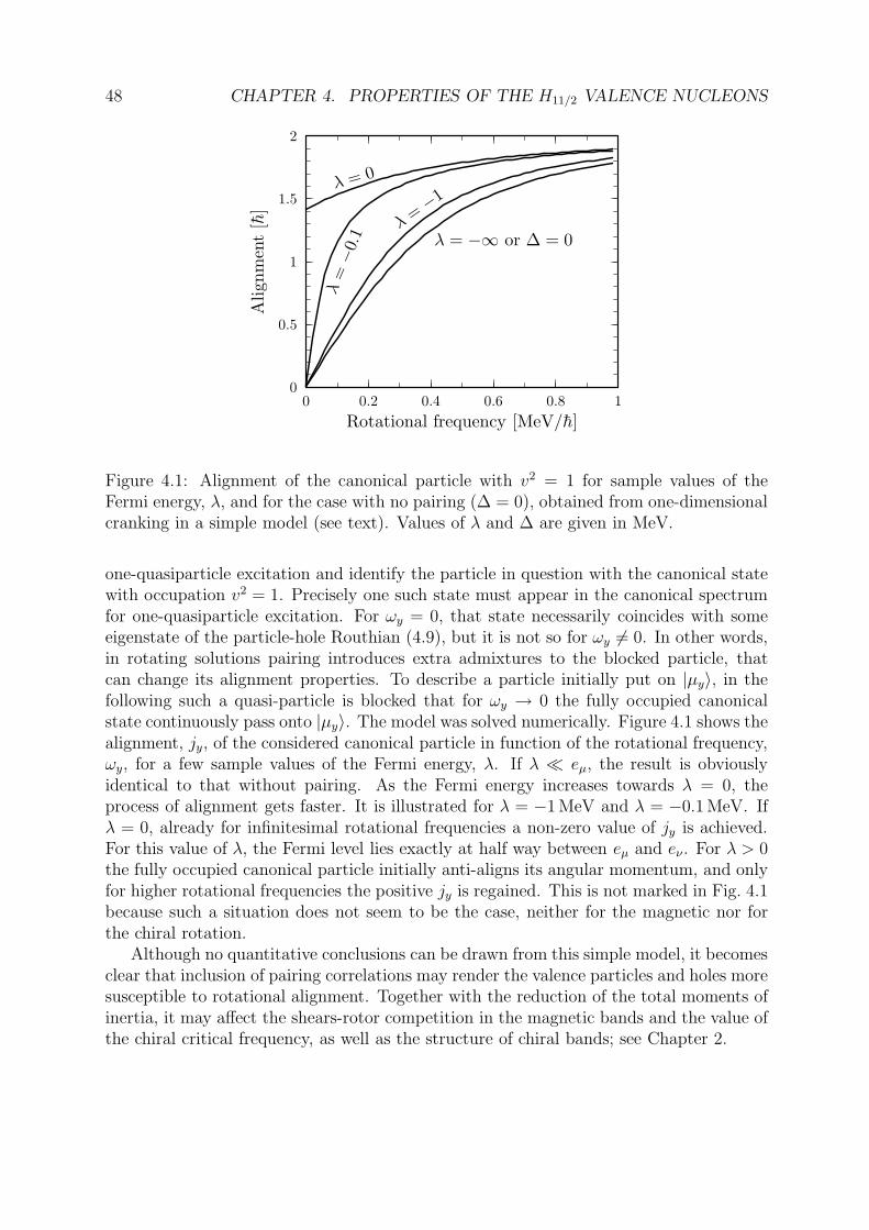
48 CHAPTER 4. PROPERTIES OF THE H11/2 VALENCE NUCLEONS
0
0.5
1
1.5
2
0 0.2 0.4 0.6 0.8 1
Ali
gnm
ent
[h]
Rotational frequency [MeV/h]
λ = −∞ or ∆ = 0λ =−1
λ=−0
.1
λ = 0
Figure 4.1: Alignment of the canonical particle with v2 = 1 for sample values of theFermi energy, λ, and for the case with no pairing (∆ = 0), obtained from one-dimensionalcranking in a simple model (see text). Values of λ and ∆ are given in MeV.
one-quasiparticle excitation and identify the particle in question with the canonical statewith occupation v2 = 1. Precisely one such state must appear in the canonical spectrumfor one-quasiparticle excitation. For ωy = 0, that state necessarily coincides with someeigenstate of the particle-hole Routhian (4.9), but it is not so for ωy 6= 0. In other words,in rotating solutions pairing introduces extra admixtures to the blocked particle, thatcan change its alignment properties. To describe a particle initially put on |µy〉, in thefollowing such a quasi-particle is blocked that for ωy → 0 the fully occupied canonicalstate continuously pass onto |µy〉. The model was solved numerically. Figure 4.1 shows thealignment, jy, of the considered canonical particle in function of the rotational frequency,ωy, for a few sample values of the Fermi energy, λ. If λ eµ, the result is obviouslyidentical to that without pairing. As the Fermi energy increases towards λ = 0, theprocess of alignment gets faster. It is illustrated for λ = −1 MeV and λ = −0.1 MeV. Ifλ = 0, already for infinitesimal rotational frequencies a non-zero value of jy is achieved.For this value of λ, the Fermi level lies exactly at half way between eµ and eν . For λ > 0the fully occupied canonical particle initially anti-aligns its angular momentum, and onlyfor higher rotational frequencies the positive jy is regained. This is not marked in Fig. 4.1because such a situation does not seem to be the case, neither for the magnetic nor forthe chiral rotation.
Although no quantitative conclusions can be drawn from this simple model, it becomesclear that inclusion of pairing correlations may render the valence particles and holes moresusceptible to rotational alignment. Together with the reduction of the total moments ofinertia, it may affect the shears-rotor competition in the magnetic bands and the value ofthe chiral critical frequency, as well as the structure of chiral bands; see Chapter 2.

Chapter 5
Hartree-Fock shears results in 142Gd
In the present work, the πh211/2 νh−2
11/2 single-particle (s.p.) configuration in 142Gd is takenas an example for the study of the shears mechanism. It is particularly simple to handle,because it involves only the well-separated h11/2 intruder orbital, and can be considereda model shears configuration. Additionally, a magnetic band supposed to be built onthat structure has been observed experimentally in 142Gd. The presented results showthe first fully self-consistent Hartree-Fock (HF) Tilted-Axis Cranking (TAC) solutions,and confirm the important role of the shears mechanism. However, the agreement withexperiment is not yet satisfactory. Possible reasons are discussed, but further research isneeded to clarify this point. A preliminary report on these results was given in [Olb02a].
5.1 Previous studies in 142Gd
Magnetic bands in 142Gd were first investigated by Sugawara et al. [Sug97a], but thepresent analysis is based on the most recent EUROBALL III measurements by Lieder etal. [Lie02a]. In that experiment, four magnetic bands, denoted DB1, DB2, DB3, DB4,were observed, and configurations of πh2
11/2 νh−211/2, πh1
11/2g−17/2 νh−2
11/2, πh211/2 νh−4
11/2 and
πh111/2g
−17/2 νh−4
11/2 were assigned to them, respectively. The present work focuses on the
DB1 structure. Figure 5.1 shows a partial level scheme of 142Gd, including the DB1 andthe ground-state band. Two ∆I = 2 bands built on the πh2
11/2 and νh−211/2 configurations
[Sta88a] are also displayed, because if the πh211/2 and νh−2
11/2 excitations are combined
together, they yield the πh211/2 νh−2
11/2 configuration of the band DB1. The πh211/2 and
νh−211/2 bandheads are 10+ isomeric states, which points to the parallel coupling of the
angular momenta of the two h11/2 proton particles and neutron holes. Such a coupling ischaracteristic for the shears mechanism; see Section 2.1.
It was discussed in Section 2.1 that deformation has a strong influence on the shearsmechanism. There is no direct experimental data on the deformation of 142Gd, but severaltheoretical predictions for the ground state are available. The Extended Thomas-Fermimethod with the Strutinsky Integral [Abo92a] gives β2 = −0.21, the Folded Yukawa po-tential combined with the Droplet Model [Mol95a] yields β2 = −0.156 and the RelativisticMean Field [Lal96a] gives β2 = −0.158. These theoretical calculations were limited toaxially-symmetric shapes. In the present work, Total Routhian Surface (TRS) calcu-
49
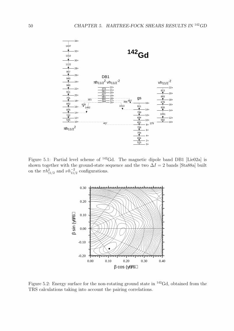
50 CHAPTER 5. HARTREE-FOCK SHEARS RESULTS IN 142GD
407
6281462
351
1013
366 667
37910+
12+
14+
16+
18+
20+
22+
24+
26+
28+
30+
32+
34+
16+17+18+19+20+21+22+
0+
2+
4+
6+
8+
10+
12+
14+
16+
10+
12+
14+
16+
18+
20+
22+
545
742
835
842
791
911
980
940
957
1122
1312
1447
373361427381301264
515
694
794
756
651
694
799
911
592
1051
826
678
893
813
πh11/22
DB1πh11/2
2 νh11/2-2
gs
νh11/2-2
142Gd
Figure 5.1: Partial level scheme of 142Gd. The magnetic dipole band DB1 [Lie02a] isshown together with the ground-state sequence and the two ∆I = 2 bands [Sta88a] builton the πh2
11/2 and νh−211/2 configurations.
0.00 0.10 0.20 0.30 0.40
-0.20
-0.10
0.00
0.10
0.20
0.30
β cos (γ+π/6)
β si
n (γ
+π/6
)
Figure 5.2: Energy surface for the non-rotating ground state in 142Gd, obtained from theTRS calculations taking into account the pairing correlations.
5.2. HF SOLUTIONS IN 142GD 51
lations allowing for triaxial deformations were performed with the pairing correlationsincluded; see Appendix C for details. The obtained energy surface is shown in Fig. 5.2.The minimum corresponds to a triaxial shape with γ ≈ 30. At γ = 0 and γ = 60
there are saddle-points, and the one for γ = 60 has lower energy, in agreement withthe previous predictions of oblate shapes. The triaxial minimum is rather shallow in theγ direction, so one can talk about γ-softness. Both the minima and the saddle-pointshave the absolute deformation of β ≈ 0.181, placing the TRS prediction between thoseof [Mol95a, Lal96a] and that of [Abo92a]. For the magnetic bands in 142Gd, phenomeno-logical TAC calculations allowing for triaxial shapes were performed in the experimentalpaper [Lie02a], by using the code of Frauendorf; see Section 3.5. Energy minimizationgave β ≈ 0.15 and γ ≈ 60 for all the four bands, but β ≈ 0.10 and γ = 60 was takenfor the cranking description of DB1 and DB3. A satisfactory agreement with experimenthas been obtained for both the energies and the B(M1)/B(E2) ratios.
5.2 HF solutions in 142Gd
This Section describes the HF ground-state and shears solutions in 142Gd. Since this isthe first application of the Skyrme-HF TAC method developed in this work, below itis explained step-by-step how those solutions were found. Refer to Section 3.6 for thetreatment of symmetries and s.p. configurations in the code hfodd.
The HF calculations in 142Gd were performed with two Skyrme parametrizations,SLy4 [Cha97a] and SkM* [Bar82a]; see Appendix C for all details. To investigate therole of the HF time-odd densities and fields, three different sets of time-odd fields, N(no time-odd fields), G (time-odd fields responsible for a gauge invariance of the force),and T (all Skyrme time-odd fields), were included; see Section 3.4. The study of theshears mechanism was preceded by a search for the ground-state minimum. Only theparity was imposed as an unbroken symmetry. Several parity reference configurations (seeSection 3.6) were considered that seemed reasonable from the standard Nilsson diagrams,with no particle-hole excitations required. Cranking constraint was applied in the firstiteration to make the calculations symmetry-unrestricted, and then released, as describedin Section 3.3. The lowest minimum was found for the parity configuration listed in thefirst row, right column of Table 5.1. With the SLy4 force, that solution corresponds to aHF vacuum, and for SkM* there is one empty positive-parity state under the last occupiednegative-parity state. It is known that the order of s.p. levels may vary from force to force.Deformation of β = 0.19, γ = 40 for SLy4 and β = 0.18, γ = 39 for SkM* was obtained.These values of β are very close to the TRS result for the ground state in 142Gd.
It should be expected that the ground state of the even-even 142Gd with quadrupoledeformation is symmetric with respect to the whole DT
2h group, not only the parity.If that was the case, each Kramers pair of a given parity would comprise two statesof opposite signatures, and the considered parity configuration would translate into aparity-signature configuration given in the first row, left column of Table 5.1. Indeed,DT
2h-imposing calculations with such a configuration were performed, and an identicalresult was obtained; see Section 3.3.
The DT2h-imposing solution was then used to examine one-dimensional rotations about
the three principal axes; see Section 4.2. Figure D.1 shows the s.p. Routhians from the
52 CHAPTER 5. HARTREE-FOCK SHEARS RESULTS IN 142GD
Table 5.1: Parity-signature and parity single-particle configurations (see Section 3.6) forprotons (π) and neutrons (ν) used to obtain the solutions in 142Gd at zero crankingfrequency.
Parity-Signature ParityRef. Exc. Ref. Exc.
142Gd SLy4 π (18,18,14,14) (36,28)Ground SkM* ν (21,21,18,18) (42,36)142Gd SLy4 π (18,18,14,14) (14– –→ 15– –) (36,28) (28 –→ 29 –)Shears SkM* ν (21,21,18,18) (18– +→ 19– +) (42,36) (36 –→ 37 –)
Principal-Axis Cranking (PAC) calculations with the SLy4 force and no time-odd fields.As it was discussed in Section 4.2, the s.p. levels 14–± to 19–± (see Section 3.6) canbe recognized as belonging to the h11/2 orbital for both kinds of nucleons. One can see,therefore, that in the considered HF solution there are two h11/2 proton particles occupyingthe lowest two-fold degenerate substate of the orbital and two h11/2 neutron holes on itshighest substate.
The considered shears band was calculated with only the parity imposed. In thelanguage of the parity configurations, the h11/2 orbital comprises states from the onedescribed by 27 – to that described by 38 –, both for neutrons and protons. With no time-odd fields, the πh2
11/2 νh−211/2 shears configuration was obtained from the ground state
by exciting one proton from the 28 – onto the 29 – state, and simultaneously promotingone neutron hole1 from 37 – onto 36 –, see the second row of Table 5.1. This led to aconverged solution for zero cranking frequency. Still with the time-odd fields switchedoff, a similar test as for the ground state was performed, showing that the mean field inthe πh2
11/2 νh−211/2 solution breaks none of the DT
2h symmetries with the parity-signatureconfiguration as specified in the second row, left column of Table 5.1.
To obtain the two-dimensional TAC solutions, a cranking frequency of 0.05 MeV/hwith equal components on the short and long axes of the nucleus was applied, startingthe iterations from the previously converged non-rotating state. For the sake of sim-plicity, the mean field obtained with the DT
2h symmetry imposed was used as a startingpoint, which guaranteed that the principal axes initially coincided with the program axes;see Section 3.3. As expected, a perpendicular coupling of the valence-nucleon angularmomenta was obtained. The band was calculated with the cranking-frequency step of0.05 MeV/h, starting the iterations for each subsequent value from the converged solutionfor the previous one.
The two occupied proton h11/2 states are marked with filled circles in Fig. D.2, showingthe s.p. Routhians for the shears band with N time-odd fields. These are just the lowesttwo h11/2 states with positive alignments on the cranking vector, as reflected by theirnegative slopes. At low frequencies, the two states have numbers 27 – and 29 –, as discussedpreviously. At ω ≈ 0.15 MeV/h, there is a crossing of the down-sloping 29 – Routhian
1Since the code hfodd works in the language of particles rather than holes, this was actually done byremoving one neutron particle from 36 –, and putting it onto 37 –.
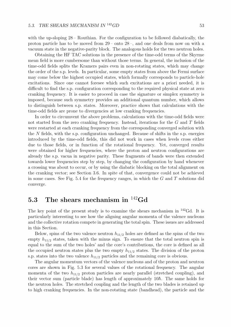
5.3. THE SHEARS MECHANISM IN 142GD 53
with the up-sloping 28 – Routhian. For the configuration to be followed diabatically, theproton particle has to be moved from 29 – onto 28 –, and one deals from now on with avacuum state in the negative-parity block. The analogous holds for the two neutron holes.
Obtaining the HF TAC solutions in the presence of the time-odd terms of the Skyrmemean field is more cumbersome than without those terms. In general, the inclusion of thetime-odd fields splits the Kramers pairs even in non-rotating states, which may changethe order of the s.p. levels. In particular, some empty states from above the Fermi surfacemay come below the highest occupied states, which formally corresponds to particle-holeexcitations. Since one cannot foresee which such excitations are a priori needed, it isdifficult to find the s.p. configuration corresponding to the required physical state at zerocranking frequency. It is easier to proceed in case the signature or simplex symmetry isimposed, because such symmetry provides an additional quantum number, which allowsto distinguish between s.p. states. Moreover, practice shows that calculations with thetime-odd fields are prone to divergencies at low cranking frequencies.
In order to circumvent the above problems, calculations with the time-odd fields werenot started from the zero cranking frequency. Instead, iterations for the G and T fieldswere restarted at each cranking frequency from the corresponding converged solution withthe N fields, with the s.p. configuration unchanged. Because of shifts in the s.p. energiesintroduced by the time-odd fields, this did not work in cases when levels cross eitherdue to those fields, or in function of the rotational frequency. Yet, converged resultswere obtained for higher frequencies, where the proton and neutron configurations arealready the s.p. vacua in negative parity. These fragments of bands were then extendedtowards lower frequencies step by step, by changing the configuration by hand whenevera crossing was about to occur, or by using the diabatic blocking on the total alignment onthe cranking vector; see Section 3.6. In spite of that, convergence could not be achievedin some cases. See Fig. 5.4 for the frequency ranges, in which the G and T solutions didconverge.
5.3 The shears mechanism in 142Gd
The key point of the present study is to examine the shears mechanism in 142Gd. It isparticularly interesting to see how the aligning angular momenta of the valence nucleonsand the collective rotation compete in generating the total spin. These issues are addressedin this Section.
Below, spins of the two valence neutron h11/2 holes are defined as the spins of the twoempty h11/2 states, taken with the minus sign. To ensure that the total neutron spin isequal to the sum of the two holes’ and the core’s contributions, the core is defined as allthe occupied neutron states plus the two empty h11/2 states. The division of the protons.p. states into the two valence h11/2 particles and the remaining core is obvious.
The angular momentum vectors of the valence nucleons and of the proton and neutroncores are shown in Fig. 5.3 for several values of the rotational frequency. The angularmomenta of the two h11/2 proton particles are nearly parallel (stretched coupling), andtheir vector sum (particle blade) has length of approximately 10h. The same holds forthe neutron holes. The stretched coupling and the length of the two blades is retained upto high cranking frequencies. In the non-rotating state (bandhead), the particle and the
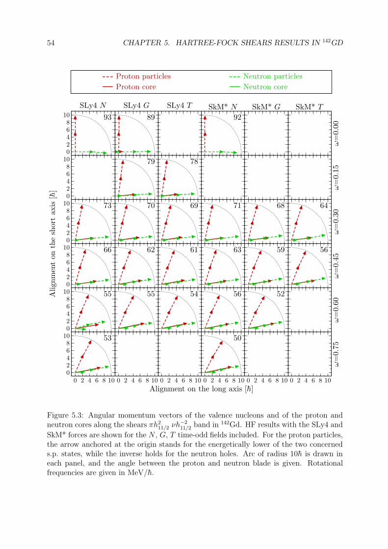
54 CHAPTER 5. HARTREE-FOCK SHEARS RESULTS IN 142GD
02468
10
SLy4 N
93
02468
10
02468
10 73
02468
10 66
02468
10 55
02468
10
0 2 4 6 8 10
53
SLy4 G
89
79
70
62
55
0 2 4 6 8 10
SLy4 T
78
69
61
54
0 2 4 6 8 10
SkM* N
92
71
63
56
0 2 4 6 8 10
50
SkM* G
68
59
52
0 2 4 6 8 10
ω=
0.0
0
SkM* T
ω=
0.1
5ω
=0.3
0
64
ω=
0.4
5
56
ω=
0.6
0
0 2 4 6 8 10
ω=
0.7
5
Ali
gnm
ent
on
the
short
axis
[h]
Alignment on the long axis [h]
Proton particles
Proton core
Neutron particles
Neutron core
Figure 5.3: Angular momentum vectors of the valence nucleons and of the proton andneutron cores along the shears πh2
11/2 νh−211/2 band in 142Gd. HF results with the SLy4 and
SkM* forces are shown for the N , G, T time-odd fields included. For the proton particles,the arrow anchored at the origin stands for the energetically lower of the two concerneds.p. states, while the inverse holds for the neutron holes. Arc of radius 10h is drawn ineach panel, and the angle between the proton and neutron blade is given. Rotationalfrequencies are given in MeV/h.
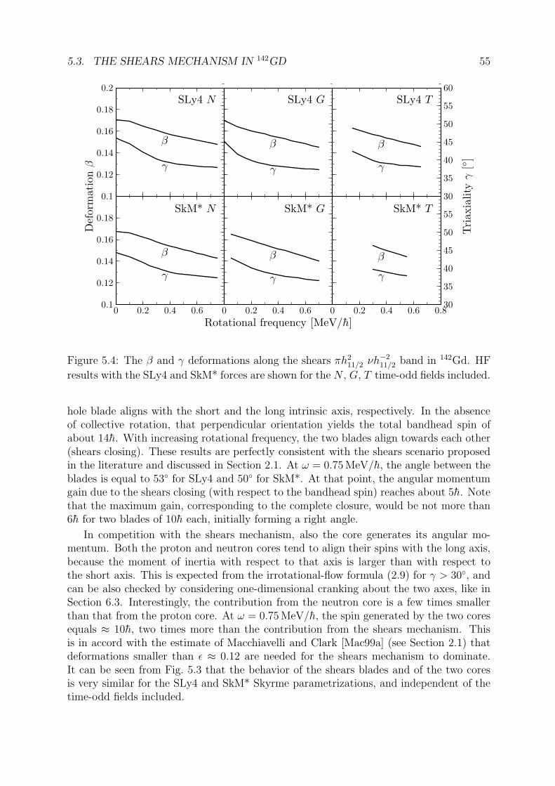
5.3. THE SHEARS MECHANISM IN 142GD 55
0.1
0.12
0.14
0.16
0.18
0.2
SLy4 N
β
SLy4 G
β
SLy4 T
β
0.1
0.12
0.14
0.16
0.18
0 0.2 0.4 0.6
SkM* N
β
0 0.2 0.4 0.6
SkM* G
β
0 0.2 0.4 0.6 0.8
SkM* T
β
γ γ
30
35
40
45
50
55
60
γ
γ γ
30
35
40
45
50
55
γ
Def
orm
ati
on
β
Tri
axia
lity
γ[
]
Rotational frequency [MeV/h]
Figure 5.4: The β and γ deformations along the shears πh211/2 νh−2
11/2 band in 142Gd. HF
results with the SLy4 and SkM* forces are shown for the N , G, T time-odd fields included.
hole blade aligns with the short and the long intrinsic axis, respectively. In the absenceof collective rotation, that perpendicular orientation yields the total bandhead spin ofabout 14h. With increasing rotational frequency, the two blades align towards each other(shears closing). These results are perfectly consistent with the shears scenario proposedin the literature and discussed in Section 2.1. At ω = 0.75 MeV/h, the angle between theblades is equal to 53 for SLy4 and 50 for SkM*. At that point, the angular momentumgain due to the shears closing (with respect to the bandhead spin) reaches about 5h. Notethat the maximum gain, corresponding to the complete closure, would be not more than6h for two blades of 10h each, initially forming a right angle.
In competition with the shears mechanism, also the core generates its angular mo-mentum. Both the proton and neutron cores tend to align their spins with the long axis,because the moment of inertia with respect to that axis is larger than with respect tothe short axis. This is expected from the irrotational-flow formula (2.9) for γ > 30, andcan be also checked by considering one-dimensional cranking about the two axes, like inSection 6.3. Interestingly, the contribution from the neutron core is a few times smallerthan that from the proton core. At ω = 0.75 MeV/h, the spin generated by the two coresequals ≈ 10h, two times more than the contribution from the shears mechanism. Thisis in accord with the estimate of Macchiavelli and Clark [Mac99a] (see Section 2.1) thatdeformations smaller than ε ≈ 0.12 are needed for the shears mechanism to dominate.It can be seen from Fig. 5.3 that the behavior of the shears blades and of the two coresis very similar for the SLy4 and SkM* Skyrme parametrizations, and independent of thetime-odd fields included.
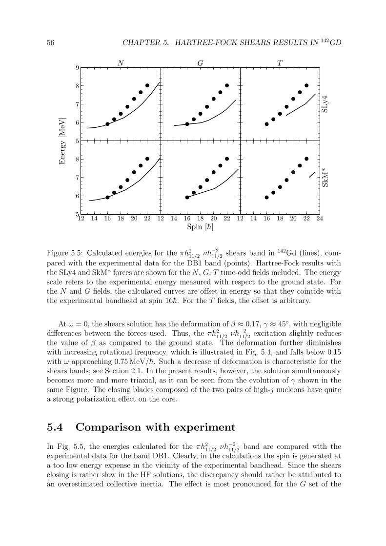
56 CHAPTER 5. HARTREE-FOCK SHEARS RESULTS IN 142GD
5
6
7
8
9N G
SL
y4
T
5
6
7
8
12 14 16 18 20 22 12 14 16 18 20 22 12 14 16 18 20 22 24
SkM
*
Ener
gy
[MeV
]
Spin [h]
Figure 5.5: Calculated energies for the πh211/2 νh−2
11/2 shears band in 142Gd (lines), com-
pared with the experimental data for the DB1 band (points). Hartree-Fock results withthe SLy4 and SkM* forces are shown for the N , G, T time-odd fields included. The energyscale refers to the experimental energy measured with respect to the ground state. Forthe N and G fields, the calculated curves are offset in energy so that they coincide withthe experimental bandhead at spin 16h. For the T fields, the offset is arbitrary.
At ω = 0, the shears solution has the deformation of β ≈ 0.17, γ ≈ 45, with negligibledifferences between the forces used. Thus, the πh2
11/2 νh−211/2 excitation slightly reduces
the value of β as compared to the ground state. The deformation further diminisheswith increasing rotational frequency, which is illustrated in Fig. 5.4, and falls below 0.15with ω approaching 0.75 MeV/h. Such a decrease of deformation is characteristic for theshears bands; see Section 2.1. In the present results, however, the solution simultaneouslybecomes more and more triaxial, as it can be seen from the evolution of γ shown in thesame Figure. The closing blades composed of the two pairs of high-j nucleons have quitea strong polarization effect on the core.
5.4 Comparison with experiment
In Fig. 5.5, the energies calculated for the πh211/2 νh−2
11/2 band are compared with theexperimental data for the band DB1. Clearly, in the calculations the spin is generated ata too low energy expense in the vicinity of the experimental bandhead. Since the shearsclosing is rather slow in the HF solutions, the discrepancy should rather be attributed toan overestimated collective inertia. The effect is most pronounced for the G set of the
5.4. COMPARISON WITH EXPERIMENT 57
time-odd fields, which systematically yields the largest values of the moments of inertia;also for the N = 75 isotones studied in Section 6.5. Apart from the time-odd fields,the moment of inertia depends strongly on the deformation and on the intensity of thepairing correlations; see Section 4.4. Since the πh2
11/2 νh−211/2 shears configuration is a
two-quasiparticle state in each kind of nucleons, the pairing effects should be significantlyweakened, and one would expect the pure HF approximation to provide a correct de-scription. From the theoretical point of view, there is no apparent reason to surmise thatthe calculated deformation is wrong, all the more since the predictions for the groundstate are consistent with the TRS results. It must be conceded, however, that the quotedestimates of [Mol95a, Lal96a] give a considerably lower β for the ground state.
Whether the combined effects of the lack of pairing in the present calculations andof a possibly overestimated deformation may account for the observed deviation fromthe experimental data should be a subject of further research. Certainly, there are stillseveral unclear points about the theoretical description of the magnetic bands in 142Gd,particularly concerning the deformation. In [Lie02a], a considerably smaller ε had to beused to reproduce the DB1 and DB3 bands than it came from the energy minimization.From the level scheme in Fig. 5.1 it is clear that the bands built on the πh2
11/2 and νh−211/2
configurations are rather well-deformed structures, similar to the ground-state band. Whywould the combination of these two excitations diminish the deformation so much? Itshould be noted here that recently Pasternak et al. [Pas04a] obtained a surprisinglygood description of the magnetic bands in 142Gd within a very simple classical model. Itwould be instructive to see whether such solutions have their self-consistent mean-fieldcounterparts.

58 CHAPTER 5. HARTREE-FOCK SHEARS RESULTS IN 142GD

Chapter 6
Hartree-Fock chiral results
Investigation of the chiral rotation in this thesis was directly stimulated by the firstexperimental observations of candidate chiral bands, in 130Cs, 132La, 134Pr, and 136Pm[Sta01b]. These nuclei were naturally chosen for the analysis in this work. An exploratorystudy performed within the Principal-Axis Cranking (PAC) revealed that a very appealingand accurate model for the chiral rotation can be given in the classical framework of twogyroscopes coupled to a triaxial rotor. That model is presented in Section 6.4 and leadsto one of the principal conclusions of this dissertation, that chiral rotation can only existabove some critical value of the rotational frequency or spin. This result is confirmedby the full Skyrme-Hartree-Fock (Skyrme-HF) solutions that are presented later in thisChapter, and constitute the first fully self-consistent proof of the chiral symmetry breakingin rotating nuclei. However, the chiral bands could be obtained only in 132La from amongthe studied isotones. A brief report on the results obtained in 132La is given in [Olb04a],which is a revised version of the e-print published earlier in [Olb02b].
6.1 Previous studies in 130Cs, 132La, 134Pr, and 136Pm
As it was discussed in Section 2.2, the πh111/2 νh−1
11/2 configuration is in the literaturecommonly adopted for the chiral doublet bands in the N = 75 isotones. Level schemes ofthose bands are displayed in Fig. 6.1. Experimental data were taken from the most recentmeasurements, namely from [Koi03a] for 130Cs, from [Sta02a, Tim03a, Gro04a] for 132La,from [Sta01b, Rob03a] for 134Pr, and from [Har01a] in the case of 136Pm. The namesof bands in 132La, B1 and B3, are reproduced from [Gro04a]. Spin assignments are stilltentative, apart from the two lowest bands in 132La. Note that the bands referred to asyrast in the present work are only yrast in the positive parity. The low-spin regions of thosebands are difficult to explore using γ-spectroscopy, because transition energies becomevery low. However, recent highbrow experiments in 132La [Tim03a] and 134Pr [Rob03a]suggested that the bandhead spins are 7+, which is consistent with the orthogonal angularmomentum coupling of the h11/2 proton particle and neutron hole. See Tables 2.1 and 2.2for a review of experimental and theoretical investigations of the chiral rotation in theN = 75 isotones.
For all of nuclei 130Cs, 132La, 134Pr, and 136Pm phenomenological Tilted-Axis Cranking(TAC) calculations were performed in [Sta01b], and in [Dim00a] also for 134Pr and in
59

60 CHAPTER 6. HARTREE-FOCK CHIRAL RESULTS
783622
688774
785827
862
1178
1141
991
865
716
7+ 8+ 9+10+
11+
12+
13+
14+
15+
16+
17+
18+
19+
20+
11+
12+
13+
14+
15+
16+
(11+)
(12+)
(13+)
(14+)
(15+)
(16+)
(17+)
(18+)
3868161294
294
392
385
454
452
506
488
558
588
777
906
994
1016
686
839
958
1046
360
380
403
427
783
916
740
830257
242
259
305
357
384
431
501
662
815
564
741
yrast
B1
B3132La
699547
595677
610
( 9+)(10+)
(11+)
(12+)
(13+)
(14+)
(15+)
(16+)
(17+)
(11+)
(12+)
(13+)
(14+)
(15+)
152
353
290
417
426
469
466
492
643
843
935
707
895
958
401
372
350
454
722
773
804
yrast
130Cs
795624
907620
944638
975559
928533
933438
910429
( 7+)( 8+)( 9+)(10+)
(11+)
(12+)
(13+)
(14+)
(15+)
(16+)
(17+)
(18+)
(19+)
(20+)
(21+)
(22+)
(23+)
(24+)
(11+)
(12+)
(13+)
(14+)
(15+)
(16+)
(17+)
(18+)
3956171287
306
416
395
495
481
546
521
539
499
440
473
475
529
593
811
976
1067
1038
913
1004
458
722
890
1027
1060
939
948
283
324
337
369
400
472
466
661
769
938
706
872
yrast
134Pr
759591
879594
666684
(8+) (9+)(10+)
(11+)
(12+)
(13+)
(14+)
(15+)
(16+)
(17+)
(18+)
(19+)
(20+)
(21+)
(11+)
(12+)
(13+)
(14+)
(15+)
(16+)
(17+)
(18+)
(19+)
(20+)
(21+)
99168285
292
408
356
478
418
506
469
456
442
437
267
577
764
896
975
898
453
700
834
924
925
879
288
364
426
424
459
435
400
434
381
403
790
883
835
815
652
850
894
834
784
yrast
136Pm
Figure 6.1: Partial level schemes of 130Cs [Koi03a], 134Pr [Sta01b, Rob03a], 136Pm[Har01a], and 132La [Sta02a, Tim03a, Gro04a], showing the yrast positive-parity bandsand supposed chiral partners. In 132La, the band B1 is the previously known partner[Sta02a], while B3 is the recently discovered third band [Gro04a].
6.2. HF MINIMA IN THE N = 75 ISOTONES 61
[Hec01a] for 136Pm. All these calculations were performed by using the TAC code ofFrauendorf. The ε deformations of 0.16, 0.175, 0.175, 0.195 and triaxialities γ of 39,32, 27, ≈ 26 were found, respectively for 130Cs, 132La, 134Pr, 136Pm. Chiral solutionswere obtained in a limited range of angular frequency. The lower limits correspond tothe critical frequency, ωcrit, discussed in this Chapter. Only [Dim00a] and [Hec01a] quotetheir values, which are ωcrit = 0.3 MeV/h for 134Pr and ωcrit < 0.2 MeV/h for 136Pm.Comparison with experimental energies is given only for 134Pr [Sta01b, Dim00a], wherethe mean trend is reproduced.
For all the considered N = 75 isotones, calculations within the Particle-Rotor Model(PRM) were performed as well [Pen03a]. A different version of the model was usedin [Har01a] for 136Pm. The same deformations were used as in the TAC calculationsdescribed in the previous Paragraph. A satisfactory agreement with experimental datawas obtained. Probably the most sophisticated implementation of the PRM was employedin 132La [Sta01a, Sta02a] and 134Pr [Sta02a]. Deformations of β = 0.23, γ = 21 andβ = 0.25, γ = 35 were adopted, respectively, and good agreement was obtained both forenergies and B(M1)/B(E2). Note that the values of β used in the latter calculations aresignificantly larger than in the former ones.
Recently, a lifetime measurement in 132La [Gro04a] provided the first data on theabsolute values of B(M1) and B(E2) in the proposed chiral bands. That experimentrevealed that the band B1, so far taken for the chiral partner, has the intraband B(E2)values an order of magnitude lower than the yrast band and than those predicted by thePRM. Moreover, a new band, called B3, was discovered, that cannot be ruled out as thechiral partner, either; see Fig. 6.14. Its electromagnetic properties are more similar tothose of the yrast band. Energetically, it is more distant form the yrast band than B1,but the spin assignments are tentative, and there are some indications [Gro04b] that theyshould be shifted up by one unit. In such a case, the band B3 would become almostexactly degenerate with the yrast sequence at spin 18 h. Certainly, further experimentalresearch is needed to clarify this point.
6.2 HF minima in the N = 75 isotones
The present HF study of 130Cs, 132La, 134Pr, and 136Pm is limited to the chiral πh111/2 νh−1
11/2
configuration. This Section describes the structure of the minima that were found for thatconfiguration before application of cranking.
Calculations were performed with two Skyrme parametrizations, SLy4 [Cha97a] andSkM* [Bar82a]; see Appendix C for all details. To investigate the role of the HF time-odddensities and fields, three different sets of time-odd fields, N (no time-odd fields), G (time-odd fields responsible for a gauge invariance of the force), and T (all Skyrme time-oddfields), were included; see Section 3.4. The πh1
11/2 νh−111/2 configuration is energetically
most favored in the mean field for the single h11/2 proton particle occupying the lowestsubstate of the orbital, and the neutron hole occupying the highest substate. Only sucha case was considered, and the HF solutions were sought much like those in 142Gd, seeSection 5.2, with the parity imposed. It was inferred from comparison of the symmetry-unrestricted and DT
2h-imposing calculations that the DT2h symmetry was not spontaneously
broken in all solutions where no time-odd fields were included. Table 6.1 gives the parity
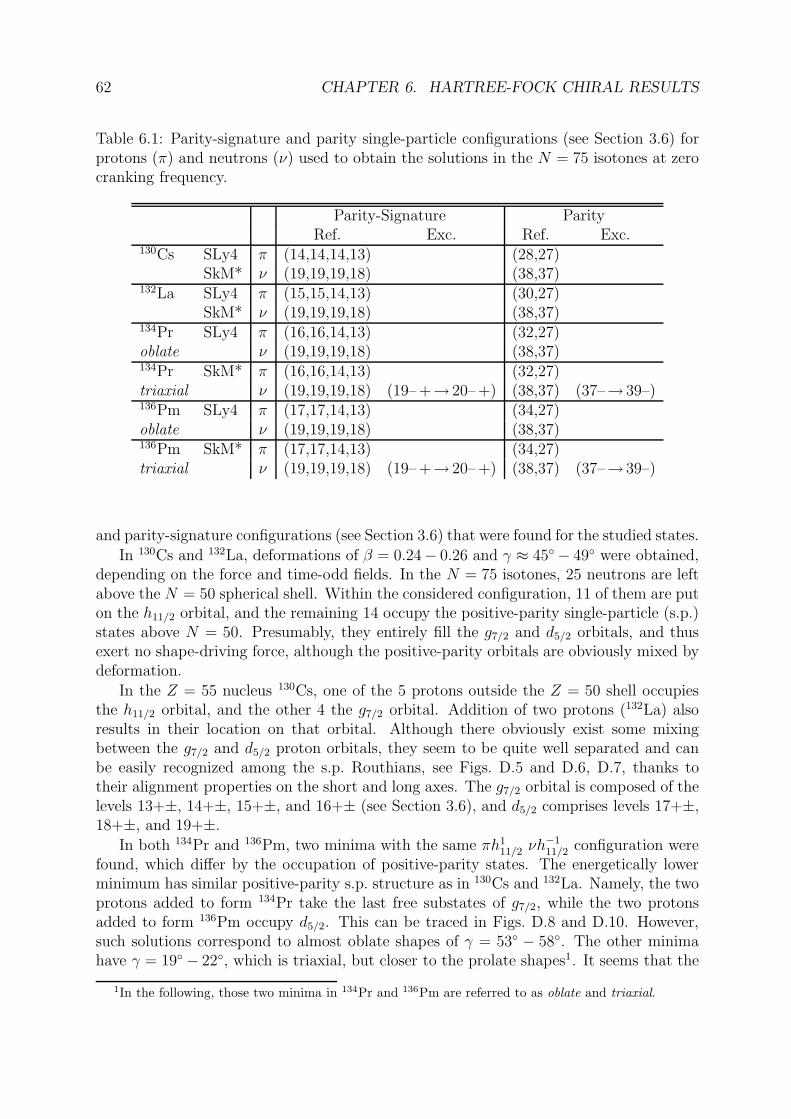
62 CHAPTER 6. HARTREE-FOCK CHIRAL RESULTS
Table 6.1: Parity-signature and parity single-particle configurations (see Section 3.6) forprotons (π) and neutrons (ν) used to obtain the solutions in the N = 75 isotones at zerocranking frequency.
Parity-Signature ParityRef. Exc. Ref. Exc.
130Cs SLy4 π (14,14,14,13) (28,27)SkM* ν (19,19,19,18) (38,37)
132La SLy4 π (15,15,14,13) (30,27)SkM* ν (19,19,19,18) (38,37)
134Pr SLy4 π (16,16,14,13) (32,27)oblate ν (19,19,19,18) (38,37)134Pr SkM* π (16,16,14,13) (32,27)triaxial ν (19,19,19,18) (19– +→ 20– +) (38,37) (37–→ 39–)136Pm SLy4 π (17,17,14,13) (34,27)oblate ν (19,19,19,18) (38,37)136Pm SkM* π (17,17,14,13) (34,27)triaxial ν (19,19,19,18) (19– +→ 20– +) (38,37) (37–→ 39–)
and parity-signature configurations (see Section 3.6) that were found for the studied states.
In 130Cs and 132La, deformations of β = 0.24− 0.26 and γ ≈ 45− 49 were obtained,depending on the force and time-odd fields. In the N = 75 isotones, 25 neutrons are leftabove the N = 50 spherical shell. Within the considered configuration, 11 of them are puton the h11/2 orbital, and the remaining 14 occupy the positive-parity single-particle (s.p.)states above N = 50. Presumably, they entirely fill the g7/2 and d5/2 orbitals, and thusexert no shape-driving force, although the positive-parity orbitals are obviously mixed bydeformation.
In the Z = 55 nucleus 130Cs, one of the 5 protons outside the Z = 50 shell occupiesthe h11/2 orbital, and the other 4 the g7/2 orbital. Addition of two protons (132La) alsoresults in their location on that orbital. Although there obviously exist some mixingbetween the g7/2 and d5/2 proton orbitals, they seem to be quite well separated and canbe easily recognized among the s.p. Routhians, see Figs. D.5 and D.6, D.7, thanks totheir alignment properties on the short and long axes. The g7/2 orbital is composed of thelevels 13+±, 14+±, 15+±, and 16+± (see Section 3.6), and d5/2 comprises levels 17+±,18+±, and 19+±.
In both 134Pr and 136Pm, two minima with the same πh111/2 νh−1
11/2 configuration werefound, which differ by the occupation of positive-parity states. The energetically lowerminimum has similar positive-parity s.p. structure as in 130Cs and 132La. Namely, the twoprotons added to form 134Pr take the last free substates of g7/2, while the two protonsadded to form 136Pm occupy d5/2. This can be traced in Figs. D.8 and D.10. However,such solutions correspond to almost oblate shapes of γ = 53 − 58. The other minimahave γ = 19 − 22, which is triaxial, but closer to the prolate shapes1. It seems that the
1In the following, those two minima in 134Pr and 136Pm are referred to as oblate and triaxial.
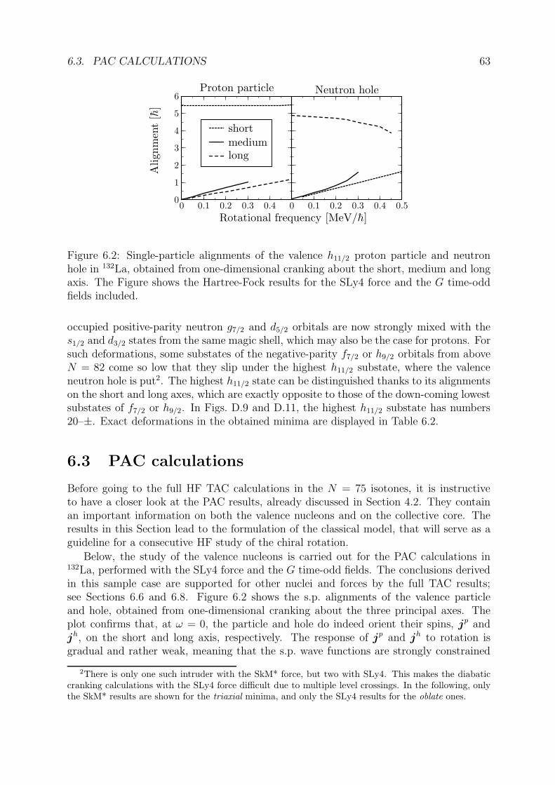
6.3. PAC CALCULATIONS 63
0
1
2
3
4
5
6
0 0.1 0.2 0.3 0.4
Proton particle
short
mediumlong
0 0.1 0.2 0.3 0.4 0.5
Neutron hole
Ali
gnm
ent
[h]
Rotational frequency [MeV/h]
Figure 6.2: Single-particle alignments of the valence h11/2 proton particle and neutronhole in 132La, obtained from one-dimensional cranking about the short, medium and longaxis. The Figure shows the Hartree-Fock results for the SLy4 force and the G time-oddfields included.
occupied positive-parity neutron g7/2 and d5/2 orbitals are now strongly mixed with thes1/2 and d3/2 states from the same magic shell, which may also be the case for protons. Forsuch deformations, some substates of the negative-parity f7/2 or h9/2 orbitals from aboveN = 82 come so low that they slip under the highest h11/2 substate, where the valenceneutron hole is put2. The highest h11/2 state can be distinguished thanks to its alignmentson the short and long axes, which are exactly opposite to those of the down-coming lowestsubstates of f7/2 or h9/2. In Figs. D.9 and D.11, the highest h11/2 substate has numbers20–±. Exact deformations in the obtained minima are displayed in Table 6.2.
6.3 PAC calculations
Before going to the full HF TAC calculations in the N = 75 isotones, it is instructiveto have a closer look at the PAC results, already discussed in Section 4.2. They containan important information on both the valence nucleons and on the collective core. Theresults in this Section lead to the formulation of the classical model, that will serve as aguideline for a consecutive HF study of the chiral rotation.
Below, the study of the valence nucleons is carried out for the PAC calculations in132La, performed with the SLy4 force and the G time-odd fields. The conclusions derivedin this sample case are supported for other nuclei and forces by the full TAC results;see Sections 6.6 and 6.8. Figure 6.2 shows the s.p. alignments of the valence particleand hole, obtained from one-dimensional cranking about the three principal axes. Theplot confirms that, at ω = 0, the particle and hole do indeed orient their spins, jp andjh, on the short and long axis, respectively. The response of jp and jh to rotation isgradual and rather weak, meaning that the s.p. wave functions are strongly constrained
2There is only one such intruder with the SkM* force, but two with SLy4. This makes the diabaticcranking calculations with the SLy4 force difficult due to multiple level crossings. In the following, onlythe SkM* results are shown for the triaxial minima, and only the SLy4 results for the oblate ones.
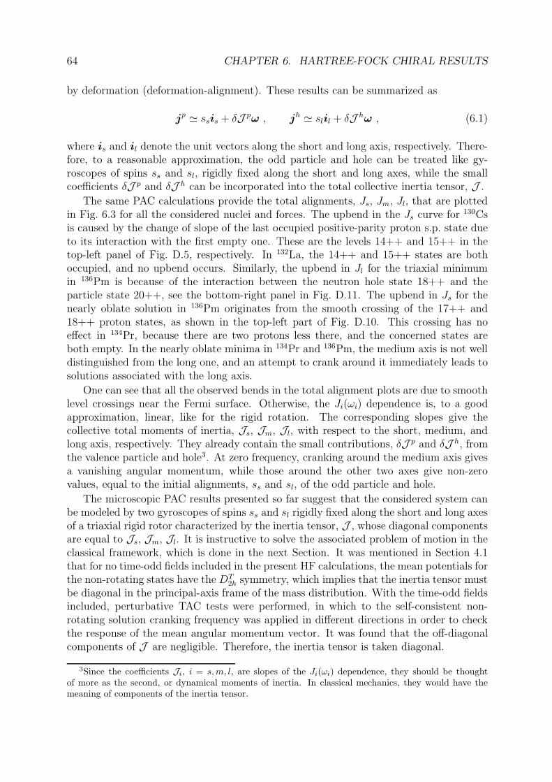
64 CHAPTER 6. HARTREE-FOCK CHIRAL RESULTS
by deformation (deformation-alignment). These results can be summarized as
jp ' ssis + δJ pω , jh ' slil + δJ hω , (6.1)
where is and il denote the unit vectors along the short and long axis, respectively. There-fore, to a reasonable approximation, the odd particle and hole can be treated like gy-roscopes of spins ss and sl, rigidly fixed along the short and long axes, while the smallcoefficients δJ p and δJ h can be incorporated into the total collective inertia tensor, J .
The same PAC calculations provide the total alignments, Js, Jm, Jl, that are plottedin Fig. 6.3 for all the considered nuclei and forces. The upbend in the Js curve for 130Csis caused by the change of slope of the last occupied positive-parity proton s.p. state dueto its interaction with the first empty one. These are the levels 14++ and 15++ in thetop-left panel of Fig. D.5, respectively. In 132La, the 14++ and 15++ states are bothoccupied, and no upbend occurs. Similarly, the upbend in Jl for the triaxial minimumin 136Pm is because of the interaction between the neutron hole state 18++ and theparticle state 20++, see the bottom-right panel in Fig. D.11. The upbend in Js for thenearly oblate solution in 136Pm originates from the smooth crossing of the 17++ and18++ proton states, as shown in the top-left part of Fig. D.10. This crossing has noeffect in 134Pr, because there are two protons less there, and the concerned states areboth empty. In the nearly oblate minima in 134Pr and 136Pm, the medium axis is not welldistinguished from the long one, and an attempt to crank around it immediately leads tosolutions associated with the long axis.
One can see that all the observed bends in the total alignment plots are due to smoothlevel crossings near the Fermi surface. Otherwise, the Ji(ωi) dependence is, to a goodapproximation, linear, like for the rigid rotation. The corresponding slopes give thecollective total moments of inertia, Js, Jm, Jl, with respect to the short, medium, andlong axis, respectively. They already contain the small contributions, δJ p and δJ h, fromthe valence particle and hole3. At zero frequency, cranking around the medium axis givesa vanishing angular momentum, while those around the other two axes give non-zerovalues, equal to the initial alignments, ss and sl, of the odd particle and hole.
The microscopic PAC results presented so far suggest that the considered system canbe modeled by two gyroscopes of spins ss and sl rigidly fixed along the short and long axesof a triaxial rigid rotor characterized by the inertia tensor, J , whose diagonal componentsare equal to Js, Jm, Jl. It is instructive to solve the associated problem of motion in theclassical framework, which is done in the next Section. It was mentioned in Section 4.1that for no time-odd fields included in the present HF calculations, the mean potentials forthe non-rotating states have the DT
2h symmetry, which implies that the inertia tensor mustbe diagonal in the principal-axis frame of the mass distribution. With the time-odd fieldsincluded, perturbative TAC tests were performed, in which to the self-consistent non-rotating solution cranking frequency was applied in different directions in order to checkthe response of the mean angular momentum vector. It was found that the off-diagonalcomponents of J are negligible. Therefore, the inertia tensor is taken diagonal.
3Since the coefficients Ji, i = s, m, l, are slopes of the Ji(ωi) dependence, they should be thoughtof more as the second, or dynamical moments of inertia. In classical mechanics, they would have themeaning of components of the inertia tensor.
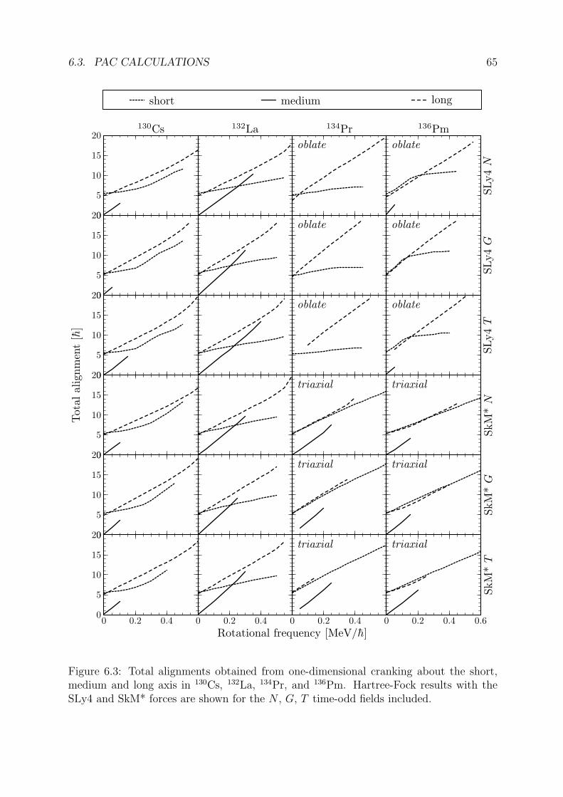
6.3. PAC CALCULATIONS 65
0
5
10
15
20130Cs
0
5
10
15
20
0
5
10
15
20
0
5
10
15
20
0
5
10
15
20
0
5
10
15
20
0 0.2 0.4
132La
0 0.2 0.4
134Pr
oblate
oblate
oblate
triaxial
triaxial
0 0.2 0.4
triaxial
SL
y4
N
136Pm
oblate
SL
y4
G
oblate
SL
y4
T
oblate
SkM
*N
triaxial
SkM
*G
triaxial
0 0.2 0.4 0.6
SkM
*T
triaxial
Tota
lali
gnm
ent
[h]
Rotational frequency [MeV/h]
short medium long
Figure 6.3: Total alignments obtained from one-dimensional cranking about the short,medium and long axis in 130Cs, 132La, 134Pr, and 136Pm. Hartree-Fock results with theSLy4 and SkM* forces are shown for the N , G, T time-odd fields included.
66 CHAPTER 6. HARTREE-FOCK CHIRAL RESULTS
JlJs
Jm
slss
Figure 6.4: The classical model of chiral rotation. Two gyroscopes of spins ss and sl
rigidly fixed along the short and long axes of a triaxial rigid body characterized by threemoments of inertia, Js, Jm, Jl, associated with the short (s), medium (m) and long (l)axis.
6.4 Classical model and the critical frequency
It was argued in the previous Section that a simple model of two gyroscopes coupled to atriaxial rigid body is appropriate for the description of rotation in the considered nuclei.Below, that model is solved in the classical framework. It possesses several analogies tothe HF TAC method in its foundations. Yet first of all, it leads to a crucial conclusionthat chiral rotation can only exist above some critical value of the rotational frequencyor spin. A simple analytical formula allows for estimating the critical frequency on thebasis of the standard PAC results.
The model system is sketched in Fig. 6.4. A triaxial rigid body models the collectivecore. Its inertia tensor, J , is diagonal with respect to the short, medium and long axes,and the corresponding components, Js, Jm, Jl, also include the small contributions fromthe valence particle and hole; see Eq. (6.1). The particle and hole are represented by twoideal gyroscopes of spins ss and sl, rigidly fixed along the short and long axis of the core,respectively.
The notion of the ideal gyroscope requires explanation. Consider an axially symmetricrigid body with moments of inertia, J‖ and J⊥, with respect to the symmetry axis andan axis perpendicular to it, respectively. If such a body spins at angular frequency Ωaround the symmetry axis, its kinetic energy is T0 = J‖Ω
2/2. Simultaneously, if thebody rotates with arbitrarily oriented frequency, ω, the kinetic energy becomes Tω =(J⊥ω2 sin2 ϑ + J‖(ω cos ϑ + Ω)2)/2, where ϑ is the angle between ω and the symmetryaxis. The ideal gyroscope is the limiting case when J‖ and J⊥ go to zero and Ω increasesso that ΩJ‖ remain constant and equal to a given value of s. Obviously the total spin isthen equal to s and points along the symmetry axis, while Tω becomes infinite. However,the difference Tω − T0 = (J⊥ sin2 ϑ + J‖ cos2 ϑ)Ω2/2 + J‖Ωω cos ϑ has a finite limit,
T = ωs cos ϑ = ωs . (6.2)
This difference can be considered as the kinetic energy of the ideal gyroscope measuredwith respect to the case with no rotation, that is with ω = 0.
6.4. CLASSICAL MODEL AND THE CRITICAL FREQUENCY 67
Coming back to the discussed classical model, the total angular momentum, J , of thesystem reads
J = Jω + s , (6.3)
where s is the vector sum of spins of the the two gyroscopes. In the absence of potentialinteractions, the Lagrangian of the system is equal to the total kinetic energy, and is givenby the formula
L = Ekin =1
2ωJω + ωs . (6.4)
Taking the laboratory components of ω as generalized velocities, it is easy to check thatthe generalized momenta are equal to the laboratory components of J . This fact allowsus to write the Legendre transformation [Gol53a] and to obtain the Hamiltonian of thesystem,
H = ωJ − L =1
2ωJω =
R2s
2Js+
R2m
2Jm+
R2l
2Jl, (6.5)
where R = J − s is the angular momentum of the rigid body alone. Note that H isanalogous to the rotational part (2.8) of the PRM Hamiltonian. Since the Lagrangian(6.4) does not depend explicite on time, Hamiltonian (6.5) is a constant of motion, andis identified with the total energy, E, of the system. Consider now a particular type ofthe Routh function [Gol53a] (Routhian), H ′, namely such that no variables undergo theLegendre transformation. In such a case, H ′ = −L, and by rewriting the Routhian interms of the Hamiltonian one obtains
H ′ = H − ωJ . (6.6)
This quantity is similar to Routhian (3.10) appearing in the quantum cranking model.Equations of motion for the model can be derived in the following way. The time
derivatives, ∂t and ∂ωt , of any vector J , taken in the laboratory frame and in a frame
rotating at angular frequency ω, respectively, are related by the formula ∂tJ = ∂ωt J+ω×J
[Gol53a]. But ∂tJ = 0, if J represents the angular momentum, which is conserved in thelaboratory frame. Thus, one obtains the Euler equations [Gol53a] for the time evolutionof the angular-momentum vector in the body-fixed frame,
∂ωt J = −ω × J . (6.7)
Thouless and Valatin [Tho62a] showed that analogous equations govern the evolution ofthe mean angular momentum in the Time-Dependent HF theory.
Apart from the equations of motion, a convenient way to analyze rotation of theconsidered system is through phase portraits, which are intersections of the angular-momentum sphere with the energy ellipsoid. Dimitrov et al. carried out such an analysis[Dim02a] for a slightly simplified version of the model. Separatrices defining the planarand chiral rotational regimes as well as the chiral vibrational regime (see Section 2.2)are clearly visible in this approach. However, the mean-field cranking approximation canonly account for the so-called uniform rotations, in which the mean angular-momentumvector is constant in the intrinsic frame of the nucleus, ∂ω
t J = 0. Because of that, also thepresent study within the classical model is limited to such uniform motions. The Eulerequations (6.7) now take the form ω×J = 0, and require that ω and J be parallel. The
68 CHAPTER 6. HARTREE-FOCK CHIRAL RESULTS
same condition holds for the HF solutions and is known as the Kerman-Onishi theorem;see Section 3.3 and [Ker81a]. These equations can be easily solved for the consideredmodel. However, to show further analogies with the HF method, here the variationalprinciple is employed to find uniform solutions.
According to the Hamilton’s principle, motion of a mechanical system can be foundby making the action integral,
∫
L dt, stationary. Here, real uniform rotations are sought,and all of them obviously belong to a wider class of trial motions with ω constant in theintrinsic frame. Within this class, Lagrangian (6.4) does not depend on time. Therefore,extremizing the action for the given ω reduces to finding extrema of the Lagrangian as afunction of the intrinsic-frame components of ω. Since H ′ = −L, the Routhian (6.6) canbe equally used for this purpose. This serves us as a bridge between the classical modeland quantum cranking theory, where an analogous Routhian is minimized in the space ofthe trial wavefunctions.
Extrema of H ′ with respect to the intrinsic-frame components of ω at a given lengthof ω can be found by using a Lagrange multiplier, µ, for ω2. Setting to zero the derivativesof the quantity
H ′ +1
2µω2 =
1
2
[
(µ−Js)ω2s + (µ− Jm)ω2
m + (µ− Jl)ω2l
]
− (ωsss + ωlsl) (6.8)
with respect to ωs, ωm, ωl, one obtains
ωs = ss/(µ−Js) , (6.9)
ωm(µ−Jm) = 0 , (6.10)
ωl = sl/(µ− Jl) . (6.11)
Equation (6.10) gives either ωm = 0 or µ = Jm, leading to two distinct classes of solutions.If ωm = 0 then both ω and J lie in the s-l plane. This gives planar solutions, for
which the chiral symmetry is not broken. All values of µ are allowed, and the Lagrangemultiplier must be determined from the length of ω calculated in the obvious way from(6.9) and (6.11). Figure 6.5a shows ω versus µ for sample model parameters, extractedfrom the HF PAC solutions with the SLy4 force with no time-odd fields, and listed inTable 6.2. The solutions marked as A and D exist for all values of ω, while above somethreshold frequency, ωthr, two more solutions appear, B and C. This threshold frequencycan be determined by finding the minimum of ω in function of µ, and reads
ωthr =
(
s2/3s + s
2/3l
)3/2
|Jl −Js|. (6.12)
The value of ωthr coming from the present HF calculations is rather high, higher than1 MeV/h. Since bands B and C are situated far above the yrast line (see Fig. 6.6) theywill not be subject of further analysis.
For µ=Jm, all values of ωm are allowed, while components in the s-l plane are fixedat ωs = ss/(Jm − Js) and ωl = sl/(Jm − Jl). Consequently, the angular momentum hasnon-zero components along all three axes, and the chiral symmetry is broken. For eachvalue of ω, there are two cases differing by the sign of ωm, and thus giving the chiral
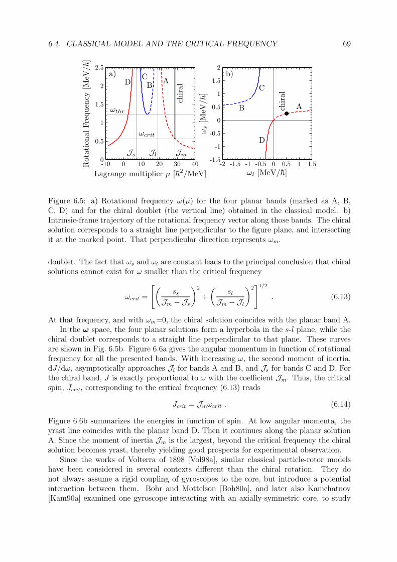
6.4. CLASSICAL MODEL AND THE CRITICAL FREQUENCY 69
0
0.5
1
1.5
2
2.5
-10 0 10 20 30 40Rota
tional
Fre
quen
cy[M
eV/h
]
Lagrange multiplier µ [h2/MeV]
DC
BA
chir
al
ωthr
ωcrit
Js JmJl
a)
-1.5
-1
-0.5
0
0.5
1
1.5
2
-2 -1.5 -1 -0.5 0 0.5 1 1.5
ωs
[MeV
/h]
ωl [MeV/h]
D
C
B Achir
al
b)
Figure 6.5: a) Rotational frequency ω(µ) for the four planar bands (marked as A, B,C, D) and for the chiral doublet (the vertical line) obtained in the classical model. b)Intrinsic-frame trajectory of the rotational frequency vector along those bands. The chiralsolution corresponds to a straight line perpendicular to the figure plane, and intersectingit at the marked point. That perpendicular direction represents ωm.
doublet. The fact that ωs and ωl are constant leads to the principal conclusion that chiralsolutions cannot exist for ω smaller than the critical frequency
ωcrit =
[
(
ss
Jm − Js
)2
+
(
sl
Jm −Jl
)2]1/2
. (6.13)
At that frequency, and with ωm=0, the chiral solution coincides with the planar band A.In the ω space, the four planar solutions form a hyperbola in the s-l plane, while the
chiral doublet corresponds to a straight line perpendicular to that plane. These curvesare shown in Fig. 6.5b. Figure 6.6a gives the angular momentum in function of rotationalfrequency for all the presented bands. With increasing ω, the second moment of inertia,dJ/dω, asymptotically approaches Jl for bands A and B, and Js for bands C and D. Forthe chiral band, J is exactly proportional to ω with the coefficient Jm. Thus, the criticalspin, Jcrit, corresponding to the critical frequency (6.13) reads
Jcrit = Jmωcrit . (6.14)
Figure 6.6b summarizes the energies in function of spin. At low angular momenta, theyrast line coincides with the planar band D. Then it continues along the planar solutionA. Since the moment of inertia Jm is the largest, beyond the critical frequency the chiralsolution becomes yrast, thereby yielding good prospects for experimental observation.
Since the works of Volterra of 1898 [Vol98a], similar classical particle-rotor modelshave been considered in several contexts different than the chiral rotation. They donot always assume a rigid coupling of gyroscopes to the core, but introduce a potentialinteraction between them. Bohr and Mottelson [Boh80a], and later also Kamchatnov[Kam90a] examined one gyroscope interacting with an axially-symmetric core, to study
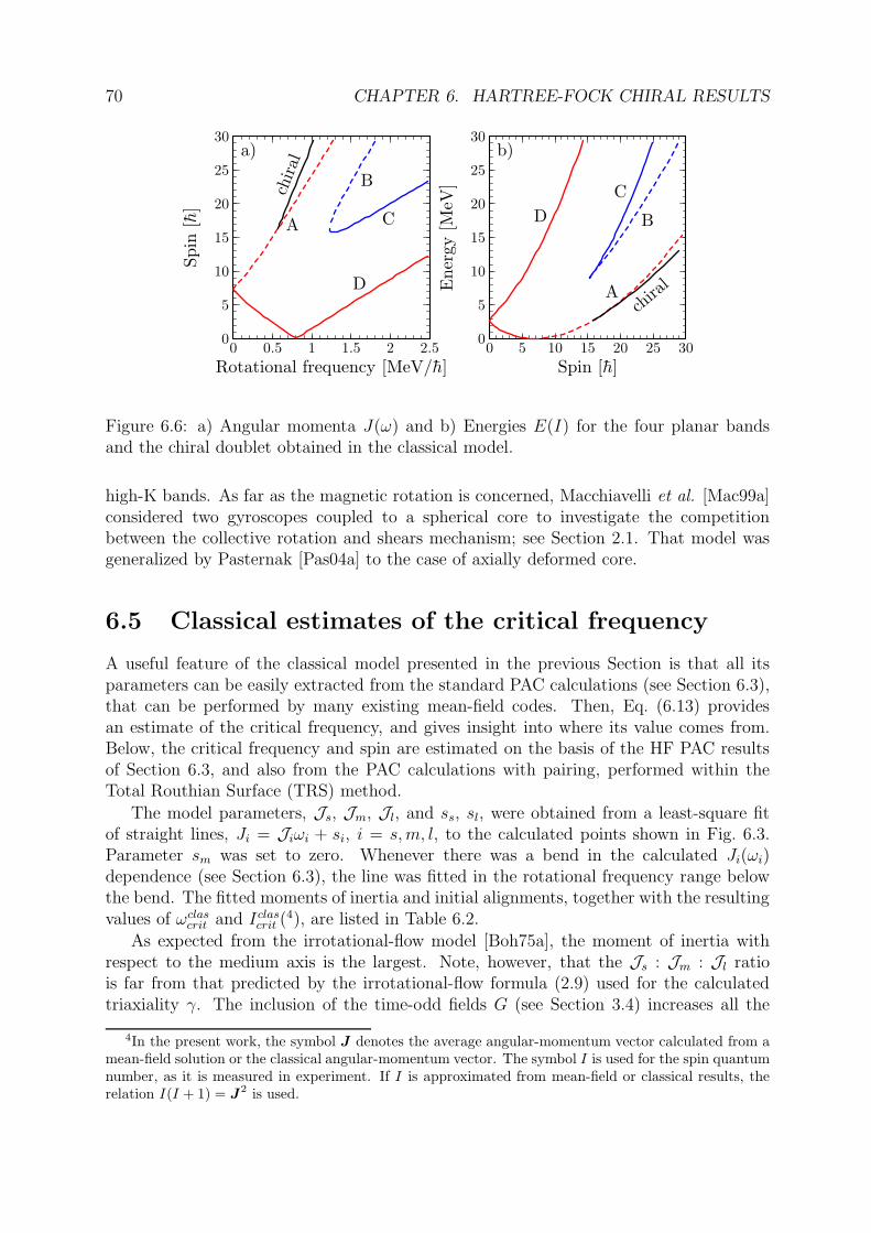
70 CHAPTER 6. HARTREE-FOCK CHIRAL RESULTS
0
5
10
15
20
25
30
0 0.5 1 1.5 2 2.5
Spin
[h]
Rotational frequency [MeV/h]
D
C
B
A
chir
al
a)
0
5
10
15
20
25
30
0 5 10 15 20 25 30
Ener
gy
[MeV
]
Spin [h]
D
C
B
Ach
iral
b)
Figure 6.6: a) Angular momenta J(ω) and b) Energies E(I) for the four planar bandsand the chiral doublet obtained in the classical model.
high-K bands. As far as the magnetic rotation is concerned, Macchiavelli et al. [Mac99a]considered two gyroscopes coupled to a spherical core to investigate the competitionbetween the collective rotation and shears mechanism; see Section 2.1. That model wasgeneralized by Pasternak [Pas04a] to the case of axially deformed core.
6.5 Classical estimates of the critical frequency
A useful feature of the classical model presented in the previous Section is that all itsparameters can be easily extracted from the standard PAC calculations (see Section 6.3),that can be performed by many existing mean-field codes. Then, Eq. (6.13) providesan estimate of the critical frequency, and gives insight into where its value comes from.Below, the critical frequency and spin are estimated on the basis of the HF PAC resultsof Section 6.3, and also from the PAC calculations with pairing, performed within theTotal Routhian Surface (TRS) method.
The model parameters, Js, Jm, Jl, and ss, sl, were obtained from a least-square fitof straight lines, Ji = Jiωi + si, i = s, m, l, to the calculated points shown in Fig. 6.3.Parameter sm was set to zero. Whenever there was a bend in the calculated Ji(ωi)dependence (see Section 6.3), the line was fitted in the rotational frequency range belowthe bend. The fitted moments of inertia and initial alignments, together with the resultingvalues of ωclas
crit and Iclascrit (4), are listed in Table 6.2.
As expected from the irrotational-flow model [Boh75a], the moment of inertia withrespect to the medium axis is the largest. Note, however, that the Js : Jm : Jl ratiois far from that predicted by the irrotational-flow formula (2.9) used for the calculatedtriaxiality γ. The inclusion of the time-odd fields G (see Section 3.4) increases all the
4In the present work, the symbol J denotes the average angular-momentum vector calculated from amean-field solution or the classical angular-momentum vector. The symbol I is used for the spin quantumnumber, as it is measured in experiment. If I is approximated from mean-field or classical results, therelation I(I + 1) = J2 is used.
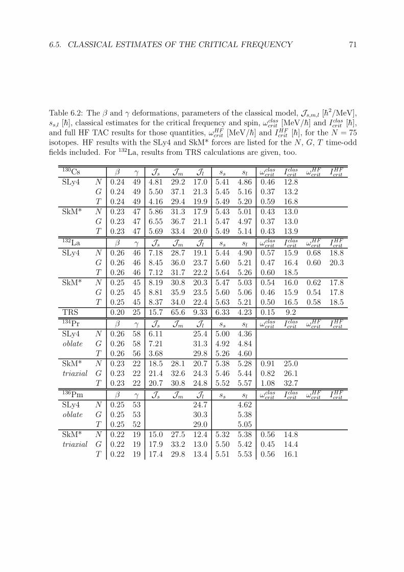
6.5. CLASSICAL ESTIMATES OF THE CRITICAL FREQUENCY 71
Table 6.2: The β and γ deformations, parameters of the classical model, Js,m,l [h2/MeV],ss,l [h], classical estimates for the critical frequency and spin, ωclas
crit [MeV/h] and Iclascrit [h],
and full HF TAC results for those quantities, ωHFcrit [MeV/h] and IHF
crit [h], for the N = 75isotopes. HF results with the SLy4 and SkM* forces are listed for the N , G, T time-oddfields included. For 132La, results from TRS calculations are given, too.
130Cs β γ Js Jm Jl ss sl ωclascrit Iclas
crit ωHFcrit IHF
crit
SLy4 N 0.24 49 4.81 29.2 17.0 5.41 4.86 0.46 12.8G 0.24 49 5.50 37.1 21.3 5.45 5.16 0.37 13.2T 0.24 49 4.16 29.4 19.9 5.49 5.20 0.59 16.8
SkM* N 0.23 47 5.86 31.3 17.9 5.43 5.01 0.43 13.0G 0.23 47 6.55 36.7 21.1 5.47 4.97 0.37 13.0T 0.23 47 5.69 33.4 20.0 5.49 5.14 0.43 13.9
132La β γ Js Jm Jl ss sl ωclascrit Iclas
crit ωHFcrit IHF
crit
SLy4 N 0.26 46 7.18 28.7 19.1 5.44 4.90 0.57 15.9 0.68 18.8G 0.26 46 8.45 36.0 23.7 5.60 5.21 0.47 16.4 0.60 20.3T 0.26 46 7.12 31.7 22.2 5.64 5.26 0.60 18.5
SkM* N 0.25 45 8.19 30.8 20.3 5.47 5.03 0.54 16.0 0.62 17.8G 0.25 45 8.81 35.9 23.5 5.60 5.06 0.46 15.9 0.54 17.8T 0.25 45 8.37 34.0 22.4 5.63 5.21 0.50 16.5 0.58 18.5
TRS 0.20 25 15.7 65.6 9.33 6.33 4.23 0.15 9.2134Pr β γ Js Jm Jl ss sl ωclas
crit Iclascrit ωHF
crit IHFcrit
SLy4 N 0.26 58 6.11 25.4 5.00 4.36oblate G 0.26 58 7.21 31.3 4.92 4.84
T 0.26 56 3.68 29.8 5.26 4.60SkM* N 0.23 22 18.5 28.1 20.7 5.38 5.28 0.91 25.0triaxial G 0.23 22 21.4 32.6 24.3 5.46 5.44 0.82 26.1
T 0.23 22 20.7 30.8 24.8 5.52 5.57 1.08 32.7136Pm β γ Js Jm Jl ss sl ωclas
crit Iclascrit ωHF
crit IHFcrit
SLy4 N 0.25 53 24.7 4.62oblate G 0.25 53 30.3 5.38
T 0.25 52 29.0 5.05SkM* N 0.22 19 15.0 27.5 12.4 5.32 5.38 0.56 14.8triaxial G 0.22 19 17.9 33.2 13.0 5.50 5.42 0.45 14.4
T 0.22 19 17.4 29.8 13.4 5.51 5.53 0.56 16.1
72 CHAPTER 6. HARTREE-FOCK CHIRAL RESULTS
moments of inertia, but particularly Jm, with respect to the case, N , with no time-oddfields. This causes a decrease in ωclas
crit , but the corresponding Iclascrit does not change much,
because Jm is larger. Switching on the fields T results in values of Jm between thoseobtained for the cases N and G. The critical frequency always becomes higher than forthe G fields, and the resulting critical spin is always the highest among all the examinedsets of time-odd fields. These variations of Iclas
crit are of the order of a few spin units.For the chiral bands in 132La, the full HF TAC solutions were found (see Section 6.8),
and the obtained values of the critical frequency and spin, ωHFcrit and IHF
crit , are also listedin Table 6.2. They are slightly higher than the classical estimates, ωclas
crit and Iclascrit , but the
agreement can be considered good, given the simplicity of the classical model. When thetime-odd fields are included, values of ωHF
crit and IHFcrit vary similarly to those of ωclas
crit andIclascrit .
To examine the possible role of pairing correlations, PAC calculations within the TRSapproach were performed for 132La; see Appendix C for details. Deformation of β ≈ 0.20and γ ≈ 25 was obtained from energy minimization. In the cranking calculations, TRSeffectively interchanges values of Js and Jl, and enlarges Jm roughly twice with respect tothe HF results. On the basis of the irrotational-flow model, these changes in the momentsof inertia can be partly understood as due to the change in triaxiality; the value of γobtained from TRS is closer to 30 and on the other side of 30 than the HF results.As governed by Eq. (6.13), the increase in Jm significantly lowers the values of ωclas
crit
and Iclascrit , see Table 6.2. However, inclusion of pairing in the full HF TAC calculations
(Hartree-Fock-Bogolyubov method) is necessary to verify this trend.Values of the critical spin obtained from the HF calculations are rather high as com-
pared to the spin range in which the supposed chiral bands are observed in nuclei understudy. A detailed comparison with experiment is given in Section 6.9.
6.6 Planar HF bands
The next step in the HF analysis of the πh111/2 νh−1
11/2 configuration in the N = 75 isotones
was to obtain planar solutions, much similar to the shears solutions in 142Gd; see Sec-tion 5.2. They serve us as starting points in the search for the chiral bands, as describedin the next two Sections.
In the N = 75 isotones, planar solutions were found by applying a tilted crankingvector to converged non-rotating states. Since in the triaxial minima in 134Pr and 136Pm,the neutron h11/2 states interleave with other negative-parity levels (see Section 6.2), itwas very difficult to follow the proper configuration diabatically, and the planar bandsin those minima were obtained only for very low angular frequencies. Figures D.12–D.14give sample s.p. Routhians for the planar bands in 132La.
Figure 6.7 shows the angular momenta of the valence h11/2 proton particle and neutronhole for the planar bands in the studied N = 75 isotones. Results with no time-oddfields are shown, as an example, because they were found in the largest frequency range,but inclusion of the G or T fields very little alters the alignments, like it was alreadydemonstrated for the shears band in 142Gd; see Fig. 5.3. One can see that, indeed, theindividual spins of the valence nucleons are rather tightly aligned along the short and longaxis, as it was expected from the PAC calculations in Section 6.3. Interestingly, there is
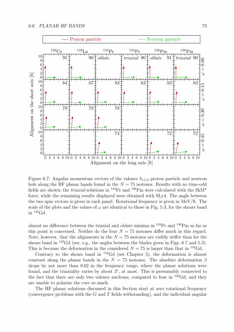
6.6. PLANAR HF BANDS 73
02468
10
130Cs
91
02468
10 84
02468
10 79
02468
10
0 2 4 6 8 10
132La
90
87
79
0 2 4 6 8 10
134Pr
oblate
83
78
0 2 4 6 8 10
74
134Pr
90triaxial
83
0 2 4 6 8 10
136Pm
91oblate
83
0 2 4 6 8 10
72
ω=
0.00
136Pm
90triaxial
ω=
0.1583
ω=
0.30
0 2 4 6 8 10
ω=
0.4572Ali
gnm
ent
on
the
short
axis
[h]
Alignment on the long axis [h]
Proton particle Neutron particle
Figure 6.7: Angular momentum vectors of the valence h11/2 proton particle and neutronhole along the HF planar bands found in the N = 75 isotones. Results with no time-oddfields are shown; the triaxial solutions in 134Pr and 136Pm were calculated with the SkM*force, while the remaining results displayed were obtained with SLy4. The angle betweenthe two spin vectors is given in each panel. Rotational frequency is given in MeV/h. Thescale of the plots and the values of ω are identical to those in Fig. 5.3, for the shears bandin 142Gd.
almost no difference between the triaxial and oblate minima in 134Pr and 136Pm as far asthis point is concerned. Neither do the four N = 75 isotones differ much in this regard.Note, however, that the alignments in the N = 75 isotones are visibly stiffer than for theshears band in 142Gd (see, e.g., the angles between the blades given in Figs. 6.7 and 5.3).This is because the deformation in the considered N = 75 is larger than that in 142Gd.
Contrary to the shears band in 142Gd (see Chapter 5), the deformation is almostconstant along the planar bands in the N = 75 isotones. The absolute deformation βdrops by not more than 0.02 in the frequency range, where the planar solutions werefound, and the triaxiality varies by about 3, at most. This is presumably connected tothe fact that there are only two valence nucleons, compared to four in 142Gd, and theyare unable to polarize the core so much.
The HF planar solutions discussed in this Section start at zero rotational frequency(convergence problems with the G and T fields withstanding), and the individual angular
74 CHAPTER 6. HARTREE-FOCK CHIRAL RESULTS
momenta of the valence particle and hole have positive projections on the ω vector. Thus,these solutions have all the characteristics of the planar band A of the classical model;see Section 6.4. Indeed, the trajectory of ω along the HF bands almost exactly followsthe classical hyperbola, as illustrated in Fig. 6.8. Also the calculated energy as functionof spin agree very well with the classical prediction, see Figs. 6.13–6.15.
6.7 Search for the chiral HF solutions
Planar HF solutions were easily obtained by applying a small cranking frequency to thenon-rotating state (at least with no time-odd fields). For chiral bands, analogous task wasmore difficult, because these bands start at a finite frequency, which in the present case isnot lower than ≈ 0.5 MeV/h. Several level crossings may occur between ω = 0 and sucha high frequency, and it is a priori difficult to identify the required s.p. configuration. Tofollow a given configuration diabatically, it is desirable to find a continuous path linkingthe chiral solution to the non-rotating state. A hint on how to proceed comes from theclassical model prediction that the chiral band sprouts from the planar solution (at thepoint corresponding to the critical frequency). One can thus restart iterations from theconverged planar band, rather than from the non-rotating state. Such a way of proceedingwas adopted in this work, to find the solutions described in the next Section. However, theauthor also found chiral solutions by performing a perturbative search along the planarband. That method gives some understanding of why chiral solutions do not appear insome cases, and therefore merits a note in this Section.
Specifically, to each converged point of the planar band, a small additional component,ωm, of the angular frequency along the medium axis was added. The resulting Routhianwas diagonalized only once, and the same parity s.p. configuration was required as for theplanar state. Then, it was checked whether in the resulting (non-selfconsistent) state theangular momentum and rotational frequency vectors were parallel or not. The Kerman-Onishi theorem [Ker81a] requires that their parallelism is a necessary condition for self-consistency; see Section 3.3. Presuming that in nuclei that are stiff against deformationchanges, the direction of J is the only degree of freedom, the Kerman-Onishi conditionis also sufficient. In other words, if J is parallel to ω in the considered state after onediagonalization, then it is very probable that further iterations may lead to a convergedchiral solution. Indeed, in practice it was always the case, and never a chiral solution wasobtained, in spite of several attempts, if that simple test gave negative result.
The condition for J and ω being parallel can be written in the form
Js
ωs
=Jm
ωm
=Jl
ωl
. (6.15)
Note that the Js/ωs and Jl/ωl ratios must be very close to each other in the non-selfconsistent state, because the Kerman-Onishi condition is fulfilled for the self-consistentplanar state. Therefore, the test consists in checking for each point of the planar band ifJm/ωm is equal to Js/ωs ≈ Jl/ωl. In fact, this is only reliable if the time-odd fields areswitched off, because in their presence, the Jm/ωm ratio calculated perturbatively is sig-nificantly smaller than the self-consistent result would be5. The test was made with ωm =
5This can be seen, e.g., from the comparison of non-selfconsistent and self-consistent PAC results. The
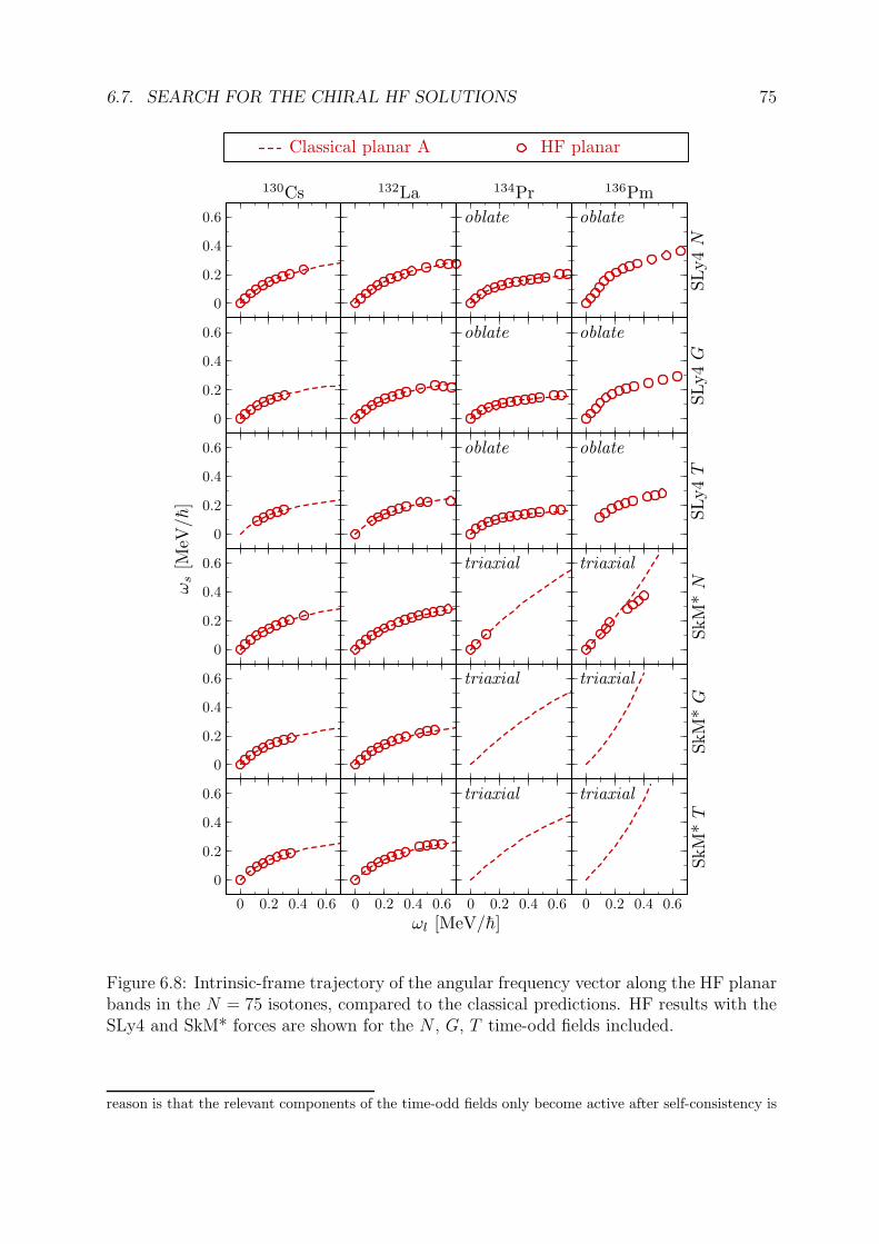
6.7. SEARCH FOR THE CHIRAL HF SOLUTIONS 75
0
0.2
0.4
0.6
130Cs
0
0.2
0.4
0.6
0
0.2
0.4
0.6
0
0.2
0.4
0.6
0
0.2
0.4
0.6
0
0.2
0.4
0.6
0 0.2 0.4 0.6
132La
0 0.2 0.4 0.6
134Pr
oblate
oblate
oblate
triaxial
triaxial
0 0.2 0.4 0.6
triaxial
SL
y4
N
136Pm
oblate
SL
y4
G
oblate
SL
y4
T
oblate
SkM
*N
triaxial
SkM
*G
triaxial
0 0.2 0.4 0.6
SkM
*T
triaxial
ωs
[MeV
/h]
ωl [MeV/h]
Classical planar A HF planar
Figure 6.8: Intrinsic-frame trajectory of the angular frequency vector along the HF planarbands in the N = 75 isotones, compared to the classical predictions. HF results with theSLy4 and SkM* forces are shown for the N , G, T time-odd fields included.
reason is that the relevant components of the time-odd fields only become active after self-consistency is
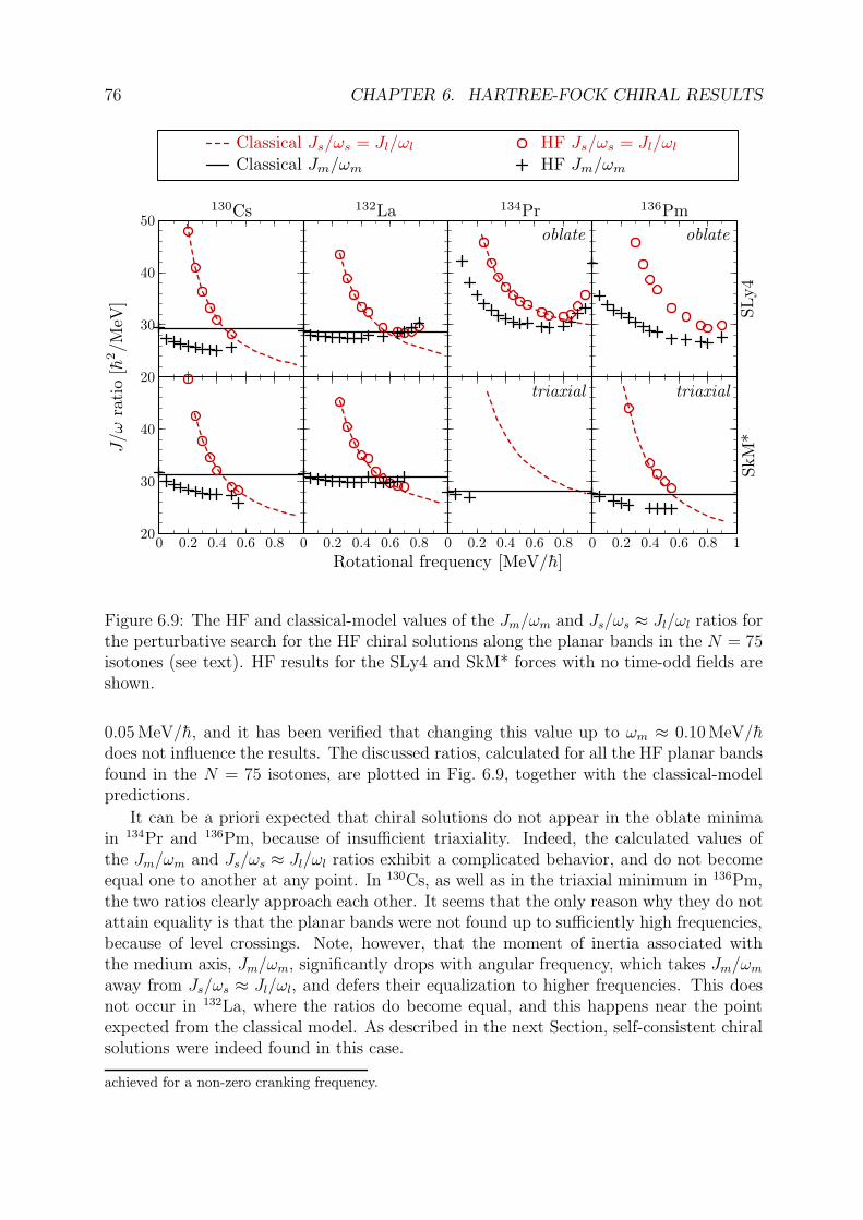
76 CHAPTER 6. HARTREE-FOCK CHIRAL RESULTS
20
30
40
50130Cs
20
30
40
0 0.2 0.4 0.6 0.8
132La
0 0.2 0.4 0.6 0.8
134Pr
oblate
0 0.2 0.4 0.6 0.8
triaxial
SL
y4
136Pm
oblate
0 0.2 0.4 0.6 0.8 1
SkM
*
triaxial
J/ω
rati
o[h
2/M
eV]
Rotational frequency [MeV/h]
Classical Js/ωs = Jl/ωl
Classical Jm/ωm
HF Js/ωs = Jl/ωl
HF Jm/ωm
Figure 6.9: The HF and classical-model values of the Jm/ωm and Js/ωs ≈ Jl/ωl ratios forthe perturbative search for the HF chiral solutions along the planar bands in the N = 75isotones (see text). HF results for the SLy4 and SkM* forces with no time-odd fields areshown.
0.05 MeV/h, and it has been verified that changing this value up to ωm ≈ 0.10 MeV/hdoes not influence the results. The discussed ratios, calculated for all the HF planar bandsfound in the N = 75 isotones, are plotted in Fig. 6.9, together with the classical-modelpredictions.
It can be a priori expected that chiral solutions do not appear in the oblate minimain 134Pr and 136Pm, because of insufficient triaxiality. Indeed, the calculated values ofthe Jm/ωm and Js/ωs ≈ Jl/ωl ratios exhibit a complicated behavior, and do not becomeequal one to another at any point. In 130Cs, as well as in the triaxial minimum in 136Pm,the two ratios clearly approach each other. It seems that the only reason why they do notattain equality is that the planar bands were not found up to sufficiently high frequencies,because of level crossings. Note, however, that the moment of inertia associated withthe medium axis, Jm/ωm, significantly drops with angular frequency, which takes Jm/ωm
away from Js/ωs ≈ Jl/ωl, and defers their equalization to higher frequencies. This doesnot occur in 132La, where the ratios do become equal, and this happens near the pointexpected from the classical model. As described in the next Section, self-consistent chiralsolutions were indeed found in this case.
achieved for a non-zero cranking frequency.
6.8. SELF-CONSISTENT CHIRAL SKYRME-HF SOLUTIONS 77
6.8 Self-consistent chiral Skyrme-HF solutions
Apart from the perturbative test described in the previous Section, self-consistent chiralsolutions were sought in the following way. To the mean field of each converged pointof the planar band, a cranking term was added with the rotational frequency of thesame magnitude as for the planar solution, but with equal components on all the threeintrinsic axes. Of course, other choices for ω are possible; the important point is tobreak the chiral symmetry at the starting point by applying a non-zero ωm, to render thecalculations symmetry-unrestricted; see Section 3.3. From the Routhian constructed insuch a way, regular HF iterations were restarted with the same parity s.p. configurationas for the planar state.
In 130Cs, 134Pr, and 136Pm, as well as for low rotational frequencies in 132La, theiterations converged to planar solutions that differed from the planar starting pointsuniquely by orientation in space (due to different direction of the applied ω). This confirmsin the frame of the Skyrme-HF method that, for the concerned configuration, the chiralsymmetry is not dynamically broken at low frequencies, as predicted by the classicalmodel. In 132La, for frequencies high enough, converged solutions were obtained with theangular momentum having non-zero components on all the three intrinsic axes, and thusviolating the chiral symmetry, RT . These are the first fully self-consistent results thatconfirm the spontaneous breaking of this symmetry in rotating atomic nuclei.
The found fragments of chiral bands were then used as starting points to obtain chiralsolutions for lower and higher angular frequencies. Calculations were performed with afrequency step of 0.02 MeV/h. At a certain value of decreasing ω, the planar orientationof the angular momentum was regained in the intrinsic frame, and the solution mergedinto the previously obtained planar band6. This confirms the classical prediction thatthe planar and chiral bands have a common point. In a natural way, that junction valueof ω can be regarded as the Skyrme-HF result for the critical frequency, and is denotedin the following as ωHF
crit . From Figs. D.12 to D.14, it can be seen that the chiral andplanar s.p. Routhians do indeed coincide at ω = ωHF
crit . Values of ωHFcrit are collected in
Table 6.2 and are discussed in the next Section. For highest frequencies, chiral solutionswere obtained up to a certain value of ω, and all attempts to go higher caused iterations tofall into another, although also chiral, minimum. This is probably due to multiple smoothcrossings of occupied and empty levels, particularly in neutrons; see the s.p. Routhians inFigs. D.12 to D.14. That other minimum is not build on the πh1
11/2 νh−111/2 configuration,
and will not be subject of further studies here. Although the chiral solutions have beenfound in a rather narrow ω interval, of about 0.1 MeV/h, the accompanying increase inωm is significant, from zero to about 0.4 MeV/h; see Fig. 6.10.
Similarly to the planar solutions described in the previous Section, there is almostno deformation change along the HF chiral bands in 132La. This yields good prospectsfor the validity of the classical descriptions of those bands; see Section 6.4. Figure 6.10gives the intrinsic-frame trajectories of the angular frequency vector along the HF chiralsolutions. In each case, the HF trajectory is almost a straight line, parallel to the medium
6With the exception of the SLy4 case with the T time-odd fields. Although a chiral solution has beenfound for this force, it could not be connected to the planar band, and it is not sure whether it is builton the πh1
11/2νh−1
11/2configuration. In the following, results for this band are not discussed.

78 CHAPTER 6. HARTREE-FOCK CHIRAL RESULTS
0
0.2
0.4
0.6
N0
0.2
0.4
0.6
ωm
[MeV
/h]
G
0
0.2
0.4
0.6
0 0.2 0.4 0.6
ωs [MeV/h]0 0.2 0.4 0.6
T
ωl [MeV/h]
0
0.2
0.4
0.6
N
0
0.2
0.4
0.6
ωm
[MeV
/h]
G
0
0.2
0.4
0.6
0 0.2 0.4 0.6
ωs [MeV/h]0 0.2 0.4 0.6
T
ωl [MeV/h]
SLy4
Classical chiral HF chiral
SkM*
Figure 6.10: Trajectory of the angular frequency vector along the HF chiral bands in132La, compared to the classical predictions. Projections onto the s-m and l-m planes ofthe intrinsic frame are shown. The Figure gives the HF results with the SLy4 and SkM*forces for the N , G, T time-odd fields included.
axis, as predicted by the classical model. The only difference is that ωHFcrit is a bit higher
than ωclascrit , and the line is shifted along the planar band to higher frequencies.
In the vicinity of ωHFcrit , the h11/2 Routhian associated with the valence neutron hole
enters a region of high density of negative-parity levels interacting among themselves.Therefore, it is doubtful whether the considered hole can still be identified with a singles.p. state. However, the h11/2 proton particle is still well separated. Figure 6.11 givesits spin alignments on the three intrinsic axes along the chiral band. The plot confirmsthe stiff character of those alignments. Like in the case of ω, only the component on themedium axis changes, the other two remaining nearly constant.
6.9 Comparison with experiment
Unfortunately, mean-field results for the chiral rotation are not directly comparable withexperimental data, as those of the PRM. This is because the pure mean-field approachdoes not take into account the interaction between the left- and right-handed solutions,which are exactly degenerate; see Section 2.2. Thus, splitting between the chiral partners
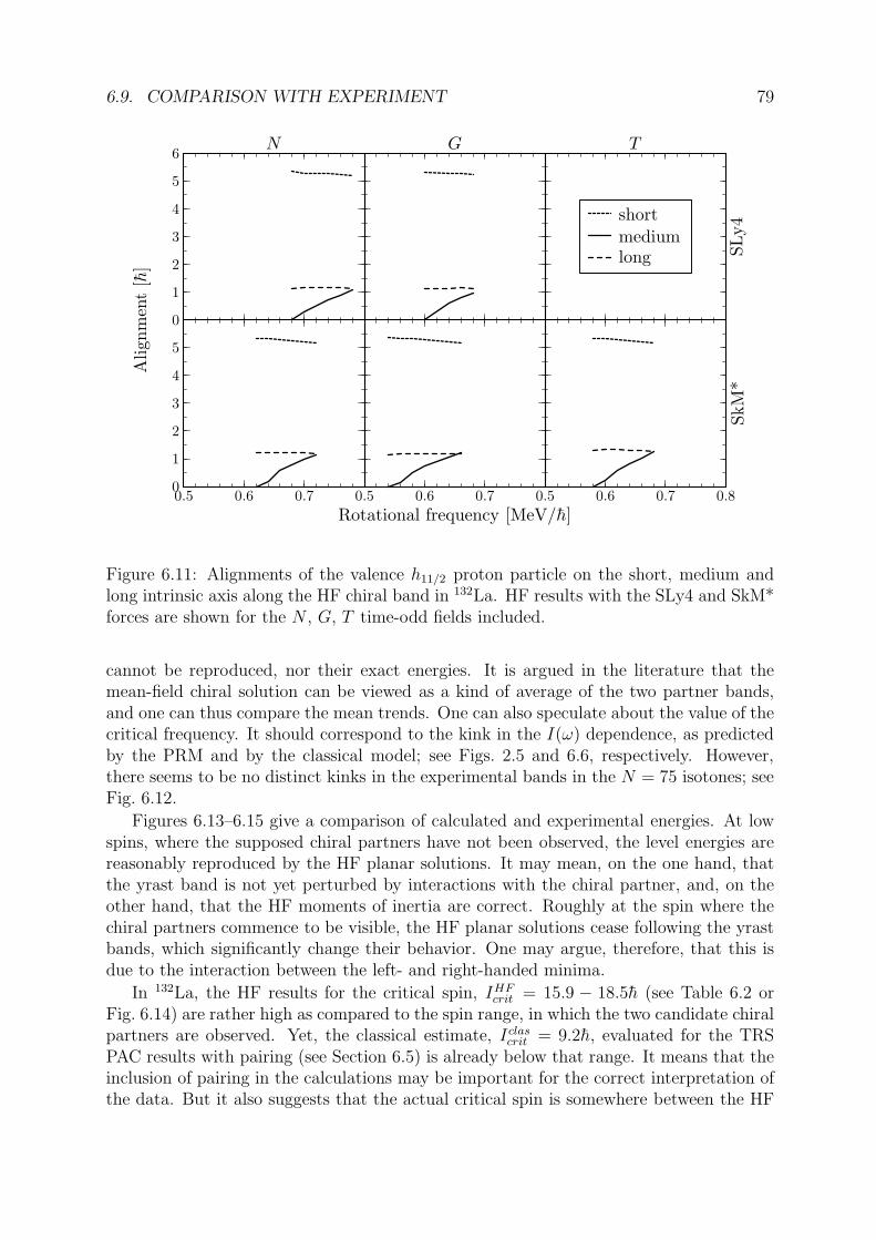
6.9. COMPARISON WITH EXPERIMENT 79
0
1
2
3
4
5
6N G
SL
y4
T
short
mediumlong
0
1
2
3
4
5
0.5 0.6 0.7 0.5 0.6 0.7 0.5 0.6 0.7 0.8
SkM
*
Ali
gnm
ent
[h]
Rotational frequency [MeV/h]
Figure 6.11: Alignments of the valence h11/2 proton particle on the short, medium andlong intrinsic axis along the HF chiral band in 132La. HF results with the SLy4 and SkM*forces are shown for the N , G, T time-odd fields included.
cannot be reproduced, nor their exact energies. It is argued in the literature that themean-field chiral solution can be viewed as a kind of average of the two partner bands,and one can thus compare the mean trends. One can also speculate about the value of thecritical frequency. It should correspond to the kink in the I(ω) dependence, as predictedby the PRM and by the classical model; see Figs. 2.5 and 6.6, respectively. However,there seems to be no distinct kinks in the experimental bands in the N = 75 isotones; seeFig. 6.12.
Figures 6.13–6.15 give a comparison of calculated and experimental energies. At lowspins, where the supposed chiral partners have not been observed, the level energies arereasonably reproduced by the HF planar solutions. It may mean, on the one hand, thatthe yrast band is not yet perturbed by interactions with the chiral partner, and, on theother hand, that the HF moments of inertia are correct. Roughly at the spin where thechiral partners commence to be visible, the HF planar solutions cease following the yrastbands, which significantly change their behavior. One may argue, therefore, that this isdue to the interaction between the left- and right-handed minima.
In 132La, the HF results for the critical spin, IHFcrit = 15.9 − 18.5h (see Table 6.2 or
Fig. 6.14) are rather high as compared to the spin range, in which the two candidate chiralpartners are observed. Yet, the classical estimate, Iclas
crit = 9.2h, evaluated for the TRSPAC results with pairing (see Section 6.5) is already below that range. It means that theinclusion of pairing in the calculations may be important for the correct interpretation ofthe data. But it also suggests that the actual critical spin is somewhere between the HF
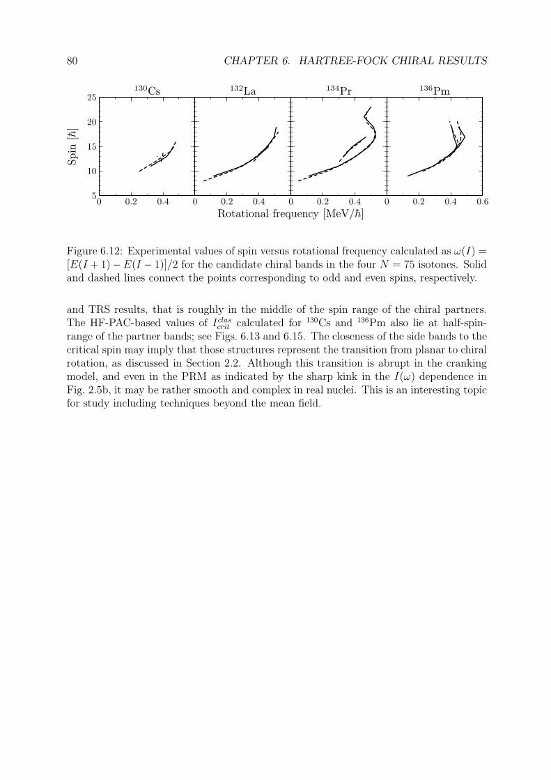
80 CHAPTER 6. HARTREE-FOCK CHIRAL RESULTS
5
10
15
20
25
0 0.2 0.4
130Cs
0 0.2 0.4
132La
0 0.2 0.4
134Pr
0 0.2 0.4 0.6
136Pm
Spin
[h]
Rotational frequency [MeV/h]
Figure 6.12: Experimental values of spin versus rotational frequency calculated as ω(I) =[E(I + 1)−E(I − 1)]/2 for the candidate chiral bands in the four N = 75 isotones. Solidand dashed lines connect the points corresponding to odd and even spins, respectively.
and TRS results, that is roughly in the middle of the spin range of the chiral partners.The HF-PAC-based values of Iclas
crit calculated for 130Cs and 136Pm also lie at half-spin-range of the partner bands; see Figs. 6.13 and 6.15. The closeness of the side bands to thecritical spin may imply that those structures represent the transition from planar to chiralrotation, as discussed in Section 2.2. Although this transition is abrupt in the crankingmodel, and even in the PRM as indicated by the sharp kink in the I(ω) dependence inFig. 2.5b, it may be rather smooth and complex in real nuclei. This is an interesting topicfor study including techniques beyond the mean field.
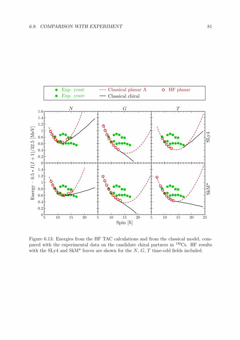
6.9. COMPARISON WITH EXPERIMENT 81
0
0.2
0.4
0.6
0.8
1
1.2
1.4
1.6N G
SL
y4
T
0
0.2
0.4
0.6
0.8
1
1.2
1.4
5 10 15 20 5 10 15 20 5 10 15 20 25
SkM
*
Ener
gy
–0.
5∗I
(I+
1)/
32.
5[M
eV]
Spin [h]
Exp. yrast
Exp. yrareClassical planar A
Classical chiral
HF planar
Figure 6.13: Energies from the HF TAC calculations and from the classical model, com-pared with the experimental data on the candidate chiral partners in 130Cs. HF resultswith the SLy4 and SkM* forces are shown for the N , G, T time-odd fields included.
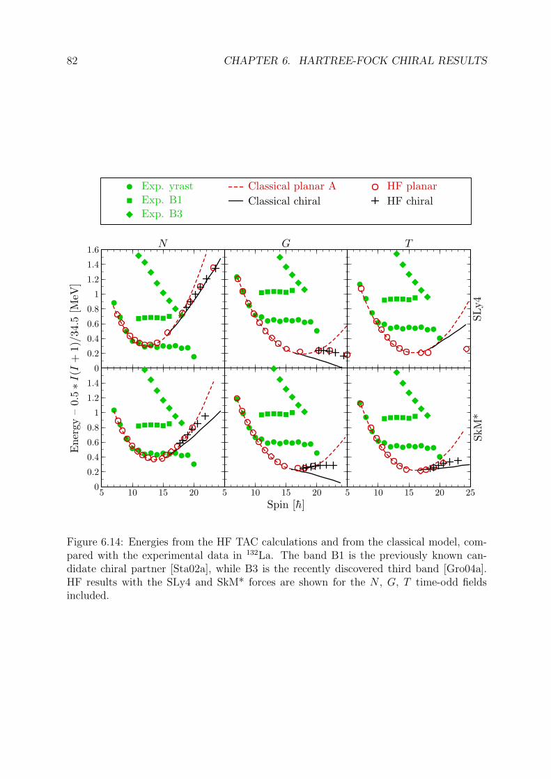
82 CHAPTER 6. HARTREE-FOCK CHIRAL RESULTS
0
0.2
0.4
0.6
0.8
1
1.2
1.4
1.6N G
SL
y4
T
0
0.2
0.4
0.6
0.8
1
1.2
1.4
5 10 15 20 5 10 15 20 5 10 15 20 25
SkM
*
Ener
gy
–0.
5∗I
(I+
1)/
34.
5[M
eV]
Spin [h]
Exp. yrast
Exp. B1
Exp. B3
Classical planar A
Classical chiral
HF planar
HF chiral
Figure 6.14: Energies from the HF TAC calculations and from the classical model, com-pared with the experimental data in 132La. The band B1 is the previously known can-didate chiral partner [Sta02a], while B3 is the recently discovered third band [Gro04a].HF results with the SLy4 and SkM* forces are shown for the N , G, T time-odd fieldsincluded.
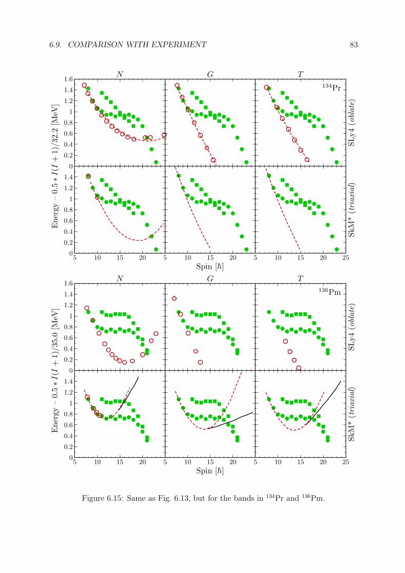
6.9. COMPARISON WITH EXPERIMENT 83
0
0.2
0.4
0.6
0.8
1
1.2
1.4
1.6N G
SL
y4
(obla
te)
T
134Pr
0
0.2
0.4
0.6
0.8
1
1.2
1.4
5 10 15 20 5 10 15 20 5 10 15 20 25
SkM
*(t
riaxia
l)
0
0.2
0.4
0.6
0.8
1
1.2
1.4
1.6N G
SL
y4
(obla
te)
T
136Pm
0
0.2
0.4
0.6
0.8
1
1.2
1.4
5 10 15 20 5 10 15 20 5 10 15 20 25
SkM
*(t
riaxia
l)
Ener
gy
–0.
5∗I
(I+
1)/
32.
2[M
eV]
Spin [h]
Ener
gy
–0.
5∗I
(I+
1)/
35.
0[M
eV]
Spin [h]
Figure 6.15: Same as Fig. 6.13, but for the bands in 134Pr and 136Pm.

84 CHAPTER 6. HARTREE-FOCK CHIRAL RESULTS
Chapter 7
Conclusions and outlook
To conclude, a numerical tool has been constructed that allows for Skyrme-Hartree-Fock (Skyrme-HF) Tilted-Axis Cranking (TAC) calculations with no symmetries imposed.Thus, it can be used for investigating the spontaneous breaking of various symmetries inrotating nuclei. As a first application, the phenomena of the magnetic and chiral rotationwere studied. For their cranking description, both two-dimensional (planar) and three-dimensional (chiral) TAC solutions were obtained, which is a robust test of the method.The present results provide one of the first fully self-consistent proofs for the possibility ofnuclear rotation about an axis tilted with respect to the principal axes. They constitutethe first fully self-consistent description of the chiral rotation, and were preceded only bya single Relativistic Mean Field calculation [Mad00a], as far as the magnetic rotation isconcerned.
Before going to the full HF TAC calculations, properties of the h11/2 valence nucleonswere examined within the PAC frame and on the basis of pure symmetry considerations.It was found that the valence particles and holes align their angular momenta alongthe short and long axis of the nucleus, respectively. It was argued that their spins arebound to those axes rather tightly, and possibly more tightly in triaxial nuclei than inaxially-symmetric ones. By considering a very simple model it was concluded that pairingcorrelations may soften those alignments.
For the study of the shears bands, the πh211/2 νh−2
11/2 configuration in 142Gd was chosen.A substantially triaxial solution was obtained. The HF results corroborate that an impor-tant portion of the angular momentum is generated by the shears mechanism, as expectedfrom earlier investigations. It was found that the aligning valence nucleons polarize thecore quite strongly, and the deformation decreases with spin. However, the rotating corealso generates angular momentum, and actually wins the competition with the shearsmechanism. This may be due to overestimated deformation or the lack of pairing in thecalculations. It is also possible that triaxiality acts against the shears mechanism by stiff-ening the alignments of the valence nucleons; such an effect has not been considered sofar. The too big collective moment of inertia causes that agreement with experiment isnot satisfactory.
The chiral solutions were sought in four N = 75 isotones, 130Cs, 132La, 134Pr, 136Pm,with the πh1
11/2 νh−111/2 configuration. Strongly triaxial solutions were found, but nearly
oblate minima proved to be lower in energy for 134Pr and 136Pm. One-dimensional crank-ing about the three axes premised that the alignments of the valence nucleons are very
85
86 CHAPTER 7. CONCLUSIONS AND OUTLOOK
stiff and that the core responds to rotation linearly, like a rigid body. On the basis ofthese results, a classical model was constructed, in which the chiral rotor is representedby two gyroscopes coupled to a triaxial rigid body. The solutions to that model agreesurprisingly well with the full HF TAC results, and elucidate the salient features of thechiral rotation. The HF chiral solutions were found only in 132La. It was established thatthe chiral rotation appears only above a certain critical value of the angular frequency; aconclusion that had been known before as a purely numerical result. In the present work,the origin of the critical frequency is explained in an illustrative way within the classicalmodel, that also gives an analytical estimate for that quantity. The HF chiral solutionscorrectly reproduce the mean E(I) behavior of the observed doublet bands in 132La. Thecalculated critical frequency is rather high as compared to the spin range in which thechiral partner bands are observed. PAC calculations with pairing suggested that pairingcorrelations may reduce its value. It is also possible that the bands in the N = 75 isotonesrepresent the transition from planar to chiral rotation.
One purpose of the present study was to investigate the influence of the Skyrme time-odd fields on the magnetic and chiral results. The inclusion of those fields changes mainlythe moments of inertia, as expected, and causes convergence problems, mainly at lowcranking frequencies. It does not alter, however, the qualitative features of the solutions.
Granted, the pairing correlations do influence the shears-rotor competition in themagnetic bands and the critical frequency in the chiral rotation. Their inclusion in theHF TAC calculations in the frame of the Hartree-Fock-Bogolyubov method would be verydesirable. The pure mean-field approach is not capable of estimating the splitting betweenthe chiral partner bands, because it does not take into account the interaction betweenthe left- and right-handed solutions. Inclusion of that interaction requires techniquesbeyond the mean field, preferably the restoration of broken chiral symmetry. To describethe smooth transition from planar to chiral rotation, it should be the projection beforevariation.
Appendix A
Invariance of the time-even density
This Appendix gives the proof that unitary mixing of states in a Kramers pair does notalter the time-even part of the density matrix, even if only one particle is put on such apair. This lemma was used in Section 4.3.
The density matrix, ρ, of an arbitrary Slater determinant, |Ψ〉, is defined as
ραβ = 〈Ψ|a+β aα|Ψ〉 . (A.1)
It can always be expressed as a sum of contributions from the single-particle (s.p.) states,|νi〉, of which |Ψ〉 is constructed,
ραβ =∑
i
〈0|aνia+
β aαa+νi|0〉 . (A.2)
The density ρ can be uniquely decomposed into a time-even part, ρ(+), and a time-oddpart, ρ(−),
ρ = ρ(+) + ρ(−) , T+ρ(+)T = +ρ(+) , T+ρ(−)T = −ρ(−) , (A.3)
in the following way:
ρ(+) =1
2(ρ + ρ) , ρ(−) =
1
2(ρ− ρ) , (A.4)
where ρ is the time-reversed density, i.e. the density of the state T |Ψ〉,
ρ = T+ρT , ραβ = (〈Ψ|T+)a+β aα(T |Ψ〉) . (A.5)
Since the time-reversal operator, T , is anti-unitary and anti-hermitian when acting on s.p.states, one can always choose the s.p. basis so that it consist of pairs of states, (|µ〉, |µ〉),mutually reversed in time up to phase factors sµ, sµ (Kramers pairs),
T |µ〉 = sµ|µ〉 , T |µ〉 = sµ|µ〉 , sµ = −sµ . (A.6)
In such a basis, the time-reversed density matrix, ρ, is related to the original density, ρ,by a simple formula,
ραβ = sαs∗βρ∗αβ . (A.7)
87
88 APPENDIX A. INVARIANCE OF THE TIME-EVEN DENSITY
See, e.g., [Dob87a] for detailed derivations.If the s.p. Hamiltonian, h, is even under transformation through the time-reversal,
T+hT = +h , (A.8)
then its eigenstates can be chosen so that they form a basis like above. The states |µ〉and |µ〉 have equal energies (Kramers degeneracy). Suppose now that of such eigenstatesone constructs a Slater determinant, |Ψ〉, and in at least one Kramers pair only one stateis occupied, say |µ〉. This may happen if the number of particles is odd or if there areparticle-hole excitations. According to (A.2), the contribution to the density matrix, ρ,from the particle on |µ〉 is
∆ραβ = 〈0|aµa+β aαa+
µ |0〉 = δαµδβµ , (A.9)
where there is no summation over µ, and ρ has been expressed in the basis of the sames.p. states, of which |Ψ〉 is built. By using (A.4) and (A.7) one finds that such a singleparticle contributes both to the time-even and to the time-odd density,
∆ρ(+)αβ =
1
2(δαµδβµ + δαµδβµ) , ∆ρ
(−)αβ =
1
2(δαµδβµ − δαµδβµ) . (A.10)
Since the states |µ〉, |µ〉 are degenerate, all their unitary combinations are equally goodeigenstates of h and can serve for constructing Slater determinants. The theorem used inSection 4.3 states that if the particle is put not on |µ〉, but on a state |µ′〉,
|µ′〉 = p|µ〉+ q|µ〉 , p∗p + q∗q = 1 , (A.11)
then its contribution to the time-even density does not change. Indeed, its new contribu-tion, ∆ρ′, to the total density equals
∆ρ′αβ = 〈0|(aµp
∗ + aµq∗)a+β aα(pa+
µ + qa+µ )|0〉 (A.12)
= p∗pδαµδβµ + p∗qδαµδβµ + q∗pδαµδβµ + q∗qδαµδβµ , (A.13)
where the same basis has been used as in (A.9). Again, from (A.4) and (A.7) one calculatesdirectly that ∆ρ′(+) = ∆ρ(+), and the time-odd term, ∆ρ(−), changes. Note yet, from(A.10), that if both states are occupied in a Kramers pair, then their contributions to thetime-odd density cancel.
Appendix B
Alignment and decoupling vectors
For a DT2 -symmetric single-particle (s.p.) Hamiltonian, the alignment and decoupling vec-
tors of eigenstates forming a Kramers pair are expressed in terms of three real parameters.Thus, the Equations (4.3, 4.4, 4.5) of Section 4.3 are derived.
Consider a Kramers pair, (|µ〉, |µ〉), as defined by (A.6). For the state |µ〉 one candefine the real alignment vector, Jµ, and the complex decoupling vector, Dµ,
Jµ = 〈µ|J |µ〉 , Dµ = 〈µ|J |µ〉 . (B.1)
Although the decoupling vector changes its phase when |µ〉, |µ〉 change their phases, therelative phases of its components do not depend on the phase convention. Since theangular-momentum operator is odd under the time reversal, it can easily be verified that
J µ = 〈µ|J |µ〉 = −Jµ , Dµ = 〈µ|J |µ〉 = Dµ ∗ . (B.2)
Here, we are concerned by properties of a single Kramers pair formed by eigenstatesof a s.p. Hamiltonian, h, that is even under the DT
2 group. Therefore, it is possible tochoose the states of the pair as eigenstates of either of the three signatures, Ri, wherei = x, y, z, but only one at a time, because the signature operators do not commuteamong themselves. This results, respectively, in three formally different pairs, (|µi〉, |µi〉),that correspond to just three different bases in the same two-dimensional eigenspace ofh. Here, it is also convened that the states |µi〉 have eigenvalues of −i under the actionof Ri, while the eigenvalues of |µi〉 are +i.
The fact that |µi〉 and |µi〉 are eigenstates of Ri, together with the transformation rulesof the components, Jj , of the angular momentum operator under the three signatures,
R+i JjRi =
+Jj j = i
−Jj j 6= i, (B.3)
induces limitations on the components, Jµi
j and Dµi
j , of the alignment and decouplingvectors. Namely,
Jµi
j =
non-zero j = i0 j 6= i
, Dµi
j =
0 j = inon-zero j 6= i
. (B.4)
In other words, Jµi is confined to the axis i and Dµi to the plane perpendicular to thataxis.
89
90 APPENDIX B. ALIGNMENT AND DECOUPLING VECTORS
In order to establish connections between the alignment and decoupling vectors as-sociated with the three pairs, (|µi〉, |µi〉), one needs to express the states of one pair aslinear combinations of those in the remaining two. Below, states |µx〉, |µx〉 and |µy〉, |µy〉are expressed as linear combinations of |µz〉, |µz〉 by diagonalization of Rx and Ry in thebasis of |µz〉, |µz〉, after having found the corresponding two-by-two matrices. Taking intoaccount that Rx and Ry are odd under Rz,
R+z RxRz = −Rx , R+
z RyRz = −Ry , (B.5)
one arrives at a conclusion that the diagonal matrix elements of Rx and Ry in the |z〉, |z〉basis vanish. The off-diagonal ones depend on the phases of |z〉, |z〉, but are restrictedby the fact that the signatures are unitary anti-hermitian operators. Moreover, the off-diagonal elements of Rx and Ry are connected by the equality
〈z|Rx|z〉 = i〈z|Ry|z〉 , (B.6)
which is due to the multiplication rule
Rx = RyRz . (B.7)
All this means that, with a proper choice of phases in |µz〉, |µz〉, one can always makethat the corresponding matrices of Ri be related to the Pauli matrices1, σi,
Ri = −iσi . (B.8)
By diagonalization of Rx and Ry one obtains, with an arbitrary choice of phases:
|µx〉 =
√
−i
2(|µz〉+ |µz〉) , |µx〉 = −
√
i
2(|µz〉 − |µz〉) , (B.9)
|µy〉 =
√
i
2(|µz〉+ i|µz〉) , |µy〉 =
√
−i
2(i|µz〉+ |µz〉) . (B.10)
These formulae, together with relations (B.2), allow to express Jµx , Dµx and Jµy , Dµy interms of Jµz , Dµz . Taking into account the constraining conditions (B.4) on the left-handside, one obtains the following set of equations:
(Jµx
x , 0, 0) = (Re Dµz
x , Re Dµz
y , 0) , (0, Dµx
y , Dµx
z ) = (−Im Dµz
x ,−Im Dµz
y ,−iJµz
z ) ,(B.11)
(0, Jµy
y , 0) = (−Im Dµz
x ,−Im Dµz
y , 0) , (Dµy
x , 0, Dµy
z ) = (−iRe Dµz
x ,−iRe Dµz
y , Jµz
z ) .(B.12)
A glance at them convinces us that all of the quantities Jµi
j , Dµi
j express through thethree ”diagonal” components, Jµi
i . One eventually arrives at:
Jµx = (Jµx
x , 0, 0) , Dµx = (0, Jµy
y ,−iJµz
z ) , (B.13)
1This assures compatibility of notation with the case of a particle possessing only the intrinsic spin andno space degrees of freedom, where the general definition, Ri = exp(−iπJi), leads explicite to Ri = −iσi.For such a particle, the states of spin | ↑〉 and | ↓〉 have the z-signature signature eigenvalues of −i and+i, respectively, and play the role of |µz〉 and |µz〉.
91
Jµy = (0, Jµy
y , 0) , Dµy = (−iJµx
x , 0, Jµz
z ) , (B.14)
Jµz = (0, 0, Jµz
z ) , Dµz = (Jµx
x ,−iJµy
y , 0) . (B.15)
If the Hamiltonian, h, has no extra symmetries, then Jµi
i can assume arbitrary values.
If h is axially symmetric, say with respect to the z axis, then the states |µz〉, |µz〉 areeigenstates of Jz, which leads to quantization of Jµz
z . In fact, Jµzz = +1/2,−3/2, ...,
because Rz = exp(−iπJz), while in the adopted convention Rz|µz〉 = −i|µz〉. For states|µx〉 and |µy〉, defined by (B.9) and (B.10), one easily finds
Jµx
x =1
2Re〈µz|J+ + J−|µz〉 , Jµy
y =1
2Re〈µz|J+ − J−|µz〉 , (B.16)
where J+ = Jx + iJy and J− = Jx − iJy are the ladder operators, that increment and
decrement the magnetic quantum number, Jz, of an eigenstate, |Jz〉, of Jz,
J+|Jz〉 ∼ |Jz + 1〉 , J−|Jz〉 ∼ |Jz − 1〉 . (B.17)
One can see, therefore, that the matrix elements in (B.16) can be non-zero only if |µz〉and |µz〉 differ in Jz by one, that is if Jµz
z = 1/2. In such a case, 〈µz|J−|µz〉 = 0, andJµx
x = Jµyy . These results can be summarized as
(Jµx
x , Jµy
y , Jµz
z ) =
(Jµ⊥
⊥ , Jµ⊥
⊥ , Jµ‖
‖ ) for Jµ‖
‖ = 1/2
(0, 0, Jµ‖
‖ ) for Jµ‖
‖ = 3/2, 5/2, ...(B.18)
The parameter Jµ⊥
⊥ is not restricted by the above kinematic conditions, and is usuallycalled decoupling parameter.

92 APPENDIX B. ALIGNMENT AND DECOUPLING VECTORS
Appendix C
Technical details of the calculations
This Appendix summarizes all technical details of the present Hartree-Fock (HF) calcu-lations, and of the auxiliary calculations performed in Chapters 5 and 6 within the TotalRouthian Surface (TRS) approach.
All the HF calculations presented in this work were performed with the help of thecode hfodd, version (v2.05c), which is described in Section 3.6. Twelve spherical shells ofthe Harmonic Oscillator were taken as the single-particle (s.p.) basis. It has been verifiedfor the one-dimensional cranking in 132La that varying the number of shells from 10 up to16 changes the quantities important for the present study, like deformation, alignments,moments of inertia, by less than 1%. The calculations were performed with two Skyrmeparameter sets, SLy4 [Cha97a] and SkM* [Bar82a]. Attempts were undertaken to obtaineach solution with three sets of the HF time-odd fields [Dob95a, Dob97a] included, aslisted in Table 3.2 and explained in Chapter 3.4. Those sets are denoted in the text as N ,G, T . Since the treatment of the pairing correlations is not yet implemented in hfodd
in the Tilted-Axis Cranking (TAC) mode, pairing was not included. In all Principal-AxisCranking (PAC) calculations, the P , Ry, ST
x , STz symmetries (and their products) were
imposed, while only P was kept in the TAC case. The respective parity-signature andparity configurations (see Section 3.6) for all the considered solutions are given in Tabs. 5.1and 6.1. The configurations were followed diabatically in each band, either by choosing theoccupied state by hand, whenever a crossing was about to occur, or by using the diabatic-blocking techniques described in Section 3.6. In all planar solutions, the direction ofω was chosen so that it had equal components on two axes of the program frame (seeSection 3.3) and zero component on the third axis. In the chiral bands, ω had equalprojections on all the three program axes. In each case, the direction of ω was kept fixed,and only its magnitude was changed. The axial and planar bands were calculated withan ω step of 0.05 MeV/h, while the step of 0.02 MeV/h was used for the chiral solutions.With no time-odd fields included, the iterations for each value of ω were restarted fromthe previously converged solution at the prior value of ω. Then, each point convergedwith no time-odd fields served as a starting point for calculations with the time-odd fieldsincluded. As explained in Section 3.6, the convergence rate is sometimes very low in TACcalculations. To deal with this difficulty, all solutions were first obtained at the levelof convergence defined by the hfodd flag EPSITE=0.000001; see the hfodd manual in[Dob00a]. Afterwards, additional iterations were repeated in portions until the functionalenergy ceased changing from one iteration to another by more than 1 eV. This criterion
93
94 APPENDIX C. TECHNICAL DETAILS OF THE CALCULATIONS
could be fulfilled after hundreds of iterations at higher frequencies, ω > 0.4 MeV/h, andafter thousands of iterations for lower frequencies, ω < 0.4 MeV/h. This process couldhave been much faster, had the technique of resetting ω parallel to J been known earlier;see Section 3.6. The constraint on ω × J was not used, because it turned out to be veryineffective; see Section 3.6.
To estimate the possible influence of the pairing correlations, auxiliary calculationswithin the TRS method were performed in the present work. In Chapter 5, the energysurface for the ground state in 142Gd was examined, and one-dimensional cranking for132La was considered in Chapter 6. The calculations were done by using the TRS softwaredeveloped by Satu la and Wyss [Sat94a]. The method employs the phenomenologicalWoods-Saxon potential and a correction for the liquid-drop energy. Self-consistency isassured in the pairing channel, and the strength of the monopole pairing is adjusted toexperimental data following the average gap method. The quadrupole pairing is alsoincluded, with the coupling constant chosen so that the pairing field possess the localgalilean invariance. Approximate projection onto good particle number is implementedwithin the Lipkin-Nogami method. The code does not allow for TAC calculations. See[Sat94a] for all details and further references.
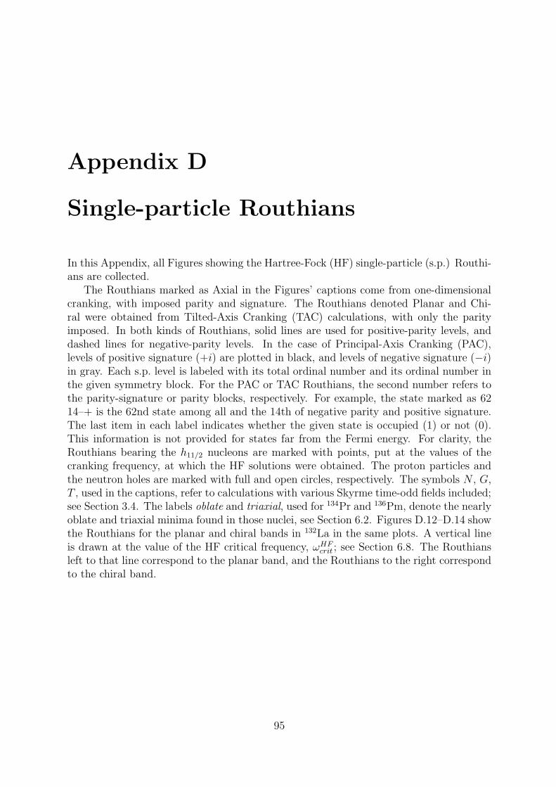
Appendix D
Single-particle Routhians
In this Appendix, all Figures showing the Hartree-Fock (HF) single-particle (s.p.) Routhi-ans are collected.
The Routhians marked as Axial in the Figures’ captions come from one-dimensionalcranking, with imposed parity and signature. The Routhians denoted Planar and Chi-ral were obtained from Tilted-Axis Cranking (TAC) calculations, with only the parityimposed. In both kinds of Routhians, solid lines are used for positive-parity levels, anddashed lines for negative-parity levels. In the case of Principal-Axis Cranking (PAC),levels of positive signature (+i) are plotted in black, and levels of negative signature (−i)in gray. Each s.p. level is labeled with its total ordinal number and its ordinal number inthe given symmetry block. For the PAC or TAC Routhians, the second number refers tothe parity-signature or parity blocks, respectively. For example, the state marked as 6214–+ is the 62nd state among all and the 14th of negative parity and positive signature.The last item in each label indicates whether the given state is occupied (1) or not (0).This information is not provided for states far from the Fermi energy. For clarity, theRouthians bearing the h11/2 nucleons are marked with points, put at the values of thecranking frequency, at which the HF solutions were obtained. The proton particles andthe neutron holes are marked with full and open circles, respectively. The symbols N , G,T , used in the captions, refer to calculations with various Skyrme time-odd fields included;see Section 3.4. The labels oblate and triaxial, used for 134Pr and 136Pm, denote the nearlyoblate and triaxial minima found in those nuclei, see Section 6.2. Figures D.12–D.14 showthe Routhians for the planar and chiral bands in 132La in the same plots. A vertical lineis drawn at the value of the HF critical frequency, ωHF
crit ; see Section 6.8. The Routhiansleft to that line correspond to the planar band, and the Routhians to the right correspondto the chiral band.
95

96 APPENDIX D. SINGLE-PARTICLE ROUTHIANS
-6
-4
-2
0
2
4Short axis
53 14++ 154 14+- 1
55 15++ 156 15+- 1
57 16++ 158 16+- 1
59 17++ 160 17+- 1
61 14– 162 14-+ 1
63 18++ 164 18+- 1
65 15– 066 15-+ 0
67 19++ 068 19+- 0
69 16– 070 16-+ 0
71 20++ 072 20+- 0
73 17– 074 17-+ 0
75 18– 076 18-+ 0
77 21++ 078 21+- 0
79 19– 080 19-+ 0
81 22++ 082 22+- 0
83 20– 084 20-+ 0
85 21– 086 21-+ 0
-16
-14
-12
-10
-8
0 0.2 0.4 0.6 0.857 16++ 158 16+- 1
59 17++ 160 17+- 1
61 14– 162 14-+ 1
63 18++ 164 18+- 1
65 19++ 166 19+- 1
67 15– 168 15-+ 1
69 16– 170 16-+ 1
71 20++ 172 20+- 1
73 17– 174 17-+ 1
75 21++ 176 21+- 1
77 18– 178 18-+ 1
79 19– 080 19-+ 0
81 22++ 082 22+- 0
83 20– 084 20-+ 0
85 21– 086 21-+ 0
87 22– 088 22-+ 0
Pro
tons
Long axis
53 14++ 154 14+- 1
55 15++ 156 15+- 1
57 16++ 158 16+- 1
59 17++ 160 17+- 1
61 14– 162 14-+ 1
63 18++ 164 18+- 1
65 15– 066 15-+ 0
67 19++ 068 19+- 0
69 16– 070 16-+ 0
71 20++ 072 20+- 0
73 17– 074 17-+ 0
75 18– 076 18-+ 0
77 21++ 078 21+- 0
79 19– 080 19-+ 0
81 22++ 082 22+- 0
83 20– 084 20-+ 0
85 21– 086 21-+ 0
0 0.2 0.4 0.6 0.8
Neu
trons
57 16++ 158 16+- 1
59 17++ 160 17+- 1
61 14– 162 14-+ 1
63 18++ 164 18+- 1
65 19++ 166 19+- 1
67 15– 168 15-+ 1
69 16– 170 16-+ 1
71 20++ 172 20+- 1
73 17– 174 17-+ 1
75 21++ 176 21+- 1
77 18– 178 18-+ 1
79 19– 080 19-+ 0
81 22++ 082 22+- 0
83 20– 084 20-+ 0
85 21– 086 21-+ 0
87 22– 088 22-+ 0
Sin
gle
-part
icle
Routh
ians
[MeV
]
Rotational frequency [MeV/h]
Figure D.1: Axial Routhians in 142Gd for SLy4 force with N time-odd fields.
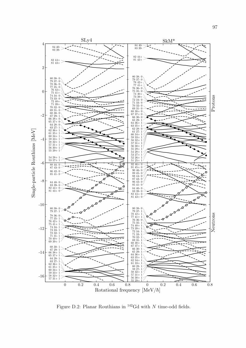
97
-6
-4
-2
0
2
4SLy4
53 27+ 154 28+ 1
55 29+ 156 30+ 157 31+ 158 32+ 159 33+ 160 34+ 161 35+ 162 36+ 163 27- 164 28- 0
65 37+ 066 38+ 067 29- 168 30- 069 31- 070 32- 071 39+72 40+
73 33- 074 34- 075 41+76 42+
77 35- 078 36- 079 37- 080 38- 0
81 43+82 44+
83 39-84 40-
-16
-14
-12
-10
-8
0 0.2 0.4 0.6 0.8
57 31+ 158 32+ 159 33+ 160 34+ 161 35+ 162 36+ 163 27- 164 28- 1
65 37+ 166 38+ 167 29- 168 30- 1
69 39+ 170 40+ 171 31- 172 32- 173 33- 174 34- 1
75 41+ 176 42+ 177 35- 178 36- 0
79 37- 180 38- 0
81 43+ 082 44+ 083 39- 084 40- 0
85 41- 086 42- 0
87 43- 088 44- 0
Pro
tons
SkM*
51 25+ 152 26+ 153 27+ 154 28+ 155 29+ 156 30+ 157 31+ 158 32+ 159 33+ 160 34+ 161 27- 162 28- 0
63 35+ 164 36+ 165 29- 166 30- 0
67 37+ 068 38+ 069 31- 070 32- 071 33- 072 34- 073 39+74 40+
75 35- 076 36- 077 41+78 42+
79 37- 080 38- 0
81 43+82 44+
83 39-84 40-
0 0.2 0.4 0.6 0.8
Neu
trons
55 29+ 156 30+ 157 31+ 158 32+ 159 27- 160 28- 1
61 33+ 162 34+ 163 35+ 164 36+ 165 29- 166 30- 1
67 37+ 168 38+ 169 31- 170 32- 171 33- 172 34- 1
73 39+ 174 40+ 175 35- 176 36- 0
77 41+ 178 42+ 179 37- 180 38- 0
81 43+ 082 44+ 083 39- 084 40- 085 41- 086 42- 087 43- 088 44- 089 45- 090 46- 0
91 45+ 092 46+ 0
Sin
gle
-part
icle
Routh
ians
[MeV
]
Rotational frequency [MeV/h]
Figure D.2: Planar Routhians in 142Gd with N time-odd fields.

98 APPENDIX D. SINGLE-PARTICLE ROUTHIANS
-6
-4
-2
0
2
4SLy4
53 27+ 154 28+ 1
55 29+ 156 30+ 157 31+ 158 32+ 159 33+ 160 34+ 161 35+ 162 27- 1
63 36+ 164 28- 0
65 37+ 066 38+ 067 29- 168 30- 069 31- 070 32- 071 39+72 40+
73 33- 074 34- 075 41+76 42+
77 35- 078 36- 079 37- 080 38- 0
81 43+82 44+
83 39-84 40-85 41-
-16
-14
-12
-10
-8
0 0.2 0.4 0.6 0.856 30+ 157 31+ 158 32+ 159 33+ 160 34+ 161 35+ 162 36+ 163 27- 164 28- 1
65 37+ 166 38+ 167 29- 168 30- 1
69 39+ 170 31- 171 32- 1
72 40+ 173 33- 1
74 41+ 175 34- 1
76 42+ 177 35- 178 36- 079 37- 1
80 38- 0
81 43+ 082 44+ 083 39- 084 40- 0
85 41- 086 42- 087 43- 088 44- 0
Pro
tons
SkM*
51 25+ 152 26+ 153 27+ 154 28+ 155 29+ 156 30+ 157 31+ 158 32+ 159 33+ 160 27- 1
61 34+ 162 35+ 163 28- 0
64 36+ 165 29- 1
66 37+ 067 30- 0
68 38+ 069 31- 070 32- 071 33- 072 39+
73 34- 074 40+
75 35- 076 41+77 42+
78 36- 079 37- 080 38- 0
81 43+82 44+
83 39-84 40-
0 0.2 0.4 0.6 0.8
Neu
trons
55 29+ 156 30+ 157 27- 1
58 31+ 159 32+ 160 33+ 161 34+ 162 35+ 163 36+ 164 28- 165 29- 1
66 37+ 167 30- 1
68 38+ 169 31- 170 32- 171 33- 1
72 39+ 173 40+ 174 34- 175 35- 1
76 41+ 177 36- 0
78 42+ 179 37- 180 38- 0
81 43+ 082 44+ 083 39- 084 40- 0
85 41- 086 42- 087 43- 0
88 45+ 089 44- 090 45- 0
Sin
gle
-part
icle
Routh
ians
[MeV
]
Rotational frequency [MeV/h]
Figure D.3: Planar Routhians in 142Gd with G time-odd fields.
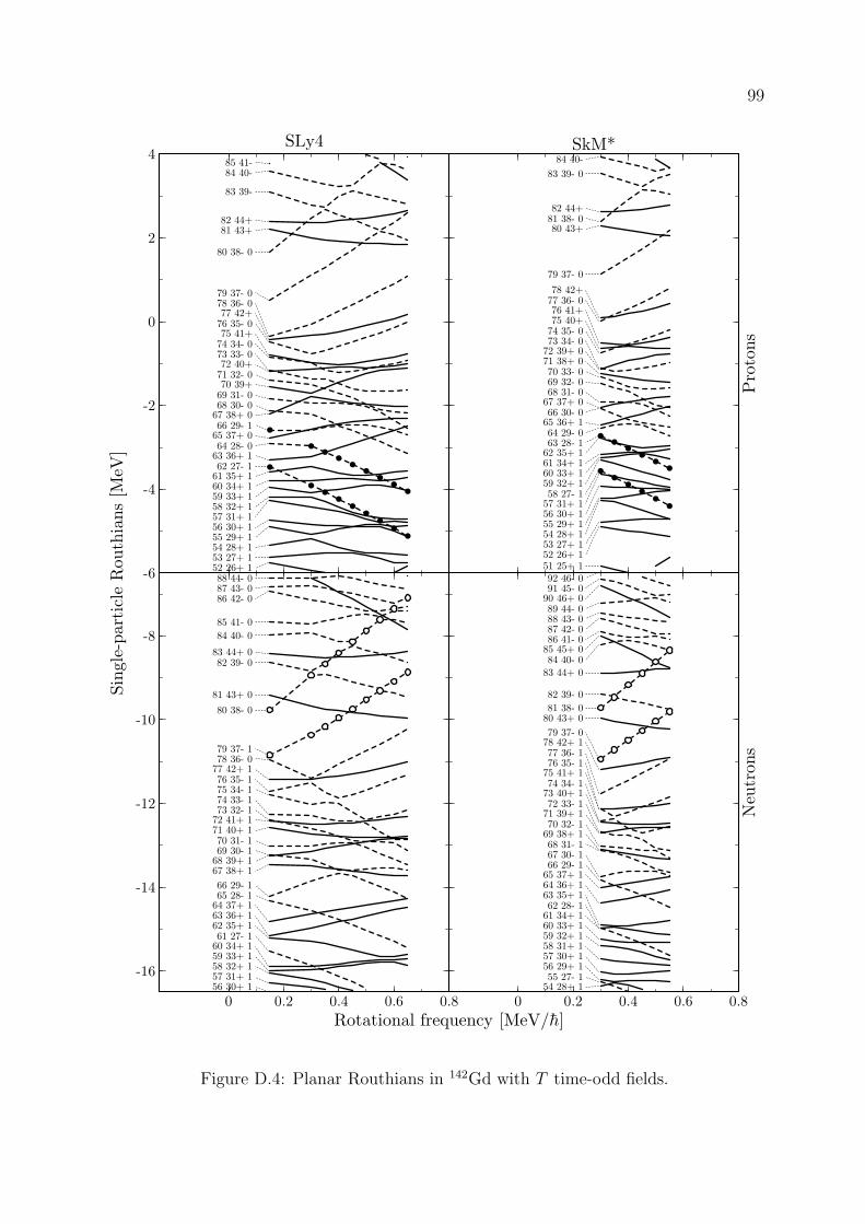
99
-6
-4
-2
0
2
4SLy4
52 26+ 153 27+ 154 28+ 155 29+ 156 30+ 157 31+ 158 32+ 159 33+ 160 34+ 161 35+ 162 27- 1
63 36+ 164 28- 0
65 37+ 066 29- 1
67 38+ 068 30- 069 31- 070 39+
71 32- 072 40+
73 33- 074 34- 075 41+
76 35- 077 42+
78 36- 079 37- 0
80 38- 0
81 43+82 44+
83 39-
84 40-85 41-
-16
-14
-12
-10
-8
0 0.2 0.4 0.6 0.856 30+ 157 31+ 158 32+ 159 33+ 160 34+ 161 27- 1
62 35+ 163 36+ 164 37+ 165 28- 166 29- 1
67 38+ 168 39+ 169 30- 170 31- 1
71 40+ 172 41+ 173 32- 174 33- 175 34- 176 35- 1
77 42+ 178 36- 079 37- 1
80 38- 0
81 43+ 0
82 39- 083 44+ 0
84 40- 0
85 41- 0
86 42- 087 43- 088 44- 0
Pro
tons
SkM*
51 25+ 152 26+ 153 27+ 154 28+ 155 29+ 156 30+ 157 31+ 158 27- 1
59 32+ 160 33+ 161 34+ 162 35+ 163 28- 164 29- 0
65 36+ 166 30- 0
67 37+ 068 31- 069 32- 070 33- 0
71 38+ 072 39+ 073 34- 074 35- 075 40+76 41+
77 36- 078 42+
79 37- 0
80 43+81 38- 082 44+
83 39- 0
84 40-
0 0.2 0.4 0.6 0.8
Neu
trons
54 28+ 155 27- 1
56 29+ 157 30+ 158 31+ 159 32+ 160 33+ 161 34+ 162 28- 1
63 35+ 164 36+ 165 37+ 166 29- 167 30- 168 31- 1
69 38+ 170 32- 1
71 39+ 172 33- 1
73 40+ 174 34- 1
75 41+ 176 35- 177 36- 1
78 42+ 179 37- 0
80 43+ 081 38- 0
82 39- 0
83 44+ 0
84 40- 085 45+ 086 41- 087 42- 088 43- 089 44- 0
90 46+ 091 45- 092 46- 0
Sin
gle
-part
icle
Routh
ians
[MeV
]
Rotational frequency [MeV/h]
Figure D.4: Planar Routhians in 142Gd with T time-odd fields.
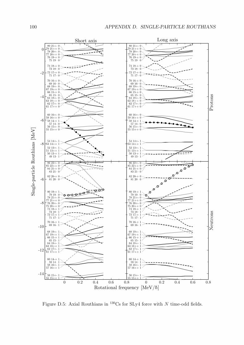
100 APPENDIX D. SINGLE-PARTICLE ROUTHIANS
-8
-6
-4
-2
0
Short axis
49 13– 150 13-+ 1
51 13++ 152 13+- 1
53 14++ 154 14+- 1
55 15++ 056 15+- 0
57 14– 058 14-+ 1
59 16++ 060 16+- 0
61 17++ 062 17+- 0
63 18++ 064 18+- 0
65 15– 066 15-+ 0
67 19++ 068 19+- 0
69 16– 070 16-+ 0
71 17– 072 17-+ 0
73 18– 074 18-+ 0
75 19– 076 19-+ 0
77 20++ 078 20+- 0
79 21++ 080 21+- 0
-14
-12
-10
-8
-6
0 0.2 0.4 0.6 0.855 15++ 156 15+- 1
57 16++ 158 16+- 1
59 14– 160 14-+ 1
61 17++ 162 17+- 1
63 18++ 164 18+- 1
65 15– 166 15-+ 1
67 19++ 168 19+- 1
69 16– 170 16-+ 1
71 17– 172 17-+ 1
73 18– 174 18-+ 1
75 20++ 076 20+- 0
77 21++ 078 21+- 0
79 19– 080 19-+ 1
81 20– 082 20-+ 0
83 21– 084 21-+ 0
85 22++ 086 22+- 0
Pro
tons
Long axis
49 13– 150 13-+ 1
51 13++ 152 13+- 1
53 14++ 154 14+- 1
55 15++ 056 15+- 0
57 14– 058 14-+ 1
59 16++ 060 16+- 0
61 17++ 062 17+- 0
63 18++ 064 18+- 0
65 15– 066 15-+ 0
67 19++ 068 19+- 0
69 16– 070 16-+ 0
71 17– 072 17-+ 0
73 18– 074 18-+ 0
75 19– 076 19-+ 0
77 20++ 078 20+- 0
79 21++ 080 21+- 0
0 0.2 0.4 0.6 0.8
Neu
trons
55 15++ 156 15+- 1
57 16++ 158 16+- 1
59 14– 160 14-+ 1
61 17++ 162 17+- 1
63 18++ 164 18+- 1
65 15– 166 15-+ 1
67 19++ 168 19+- 1
69 16– 170 16-+ 1
71 17– 172 17-+ 1
73 18– 174 18-+ 1
75 20++ 076 20+- 0
77 21++ 078 21+- 0
79 19– 080 19-+ 1
81 20– 082 20-+ 0
83 21– 084 21-+ 0
85 22++ 086 22+- 0
Sin
gle
-part
icle
Routh
ians
[MeV
]
Rotational frequency [MeV/h]
Figure D.5: Axial Routhians in 130Cs for SLy4 force with N time-odd fields.
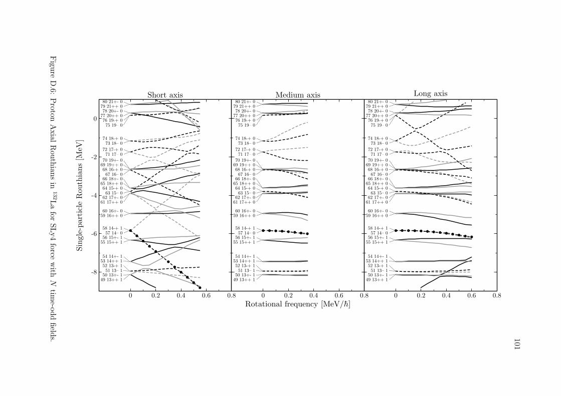
101
-8
-6
-4
-2
0
0 0.2 0.4 0.6 0.8
Short axis
49 13++ 150 13+- 1
51 13– 152 13-+ 1
53 14++ 154 14+- 1
55 15++ 156 15+- 1
57 14– 058 14-+ 1
59 16++ 060 16+- 0
61 17++ 062 17+- 0
63 15– 064 15-+ 0
65 18++ 066 18+- 0
67 16– 068 16-+ 0
69 19++ 070 19+- 0
71 17– 072 17-+ 0
73 18– 074 18-+ 0
75 19– 076 19-+ 0
77 20++ 078 20+- 0
79 21++ 080 21+- 0
0 0.2 0.4 0.6 0.8
Medium axis
49 13++ 150 13+- 1
51 13– 152 13-+ 1
53 14++ 154 14+- 1
55 15++ 156 15+- 1
57 14– 058 14-+ 1
59 16++ 060 16+- 0
61 17++ 062 17+- 0
63 15– 064 15-+ 0
65 18++ 066 18+- 0
67 16– 068 16-+ 0
69 19++ 070 19+- 0
71 17– 072 17-+ 0
73 18– 074 18-+ 0
75 19– 076 19-+ 0
77 20++ 078 20+- 0
79 21++ 080 21+- 0
0 0.2 0.4 0.6 0.8
Long axis
49 13++ 150 13+- 1
51 13– 152 13-+ 1
53 14++ 154 14+- 1
55 15++ 156 15+- 1
57 14– 058 14-+ 1
59 16++ 060 16+- 0
61 17++ 062 17+- 0
63 15– 064 15-+ 0
65 18++ 066 18+- 0
67 16– 068 16-+ 0
69 19++ 070 19+- 0
71 17– 072 17-+ 0
73 18– 074 18-+ 0
75 19– 076 19-+ 0
77 20++ 078 20+- 0
79 21++ 080 21+- 0
Sin
gle
-part
icle
Routh
ians
[MeV
]
Rotational frequency [MeV/h]
Figu
reD
.6:P
rotonA
xial
Rou
thian
sin
132L
afor
SL
y4
forcew
ithN
time-o
dd
field
s.
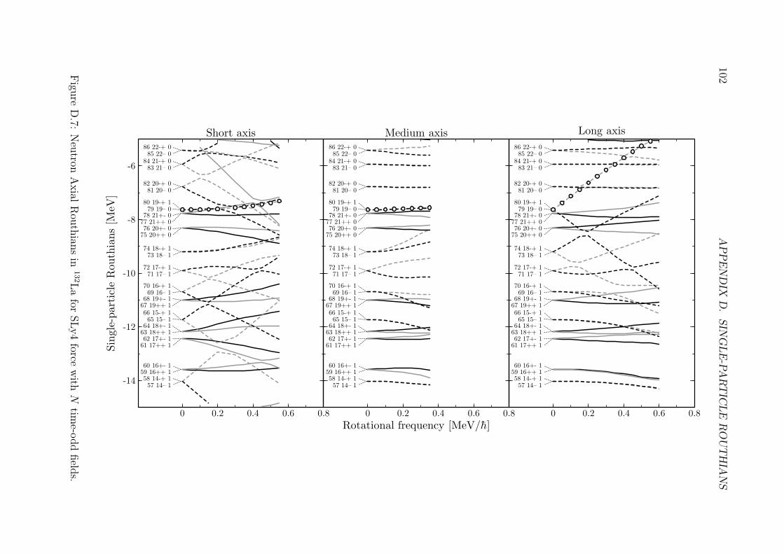
102A
PP
EN
DIX
D.
SIN
GLE
-PA
RT
ICLE
RO
UT
HIA
NS
-14
-12
-10
-8
-6
0 0.2 0.4 0.6 0.8
Short axis
57 14– 158 14-+ 1
59 16++ 160 16+- 1
61 17++ 162 17+- 1
63 18++ 164 18+- 1
65 15– 166 15-+ 1
67 19++ 168 19+- 1
69 16– 170 16-+ 1
71 17– 172 17-+ 1
73 18– 174 18-+ 1
75 20++ 076 20+- 0
77 21++ 078 21+- 0
79 19– 080 19-+ 1
81 20– 082 20-+ 0
83 21– 084 21-+ 0
85 22– 086 22-+ 0
0 0.2 0.4 0.6 0.8
Medium axis
57 14– 158 14-+ 1
59 16++ 160 16+- 1
61 17++ 162 17+- 1
63 18++ 164 18+- 1
65 15– 166 15-+ 1
67 19++ 168 19+- 1
69 16– 170 16-+ 1
71 17– 172 17-+ 1
73 18– 174 18-+ 1
75 20++ 076 20+- 0
77 21++ 078 21+- 0
79 19– 080 19-+ 1
81 20– 082 20-+ 0
83 21– 084 21-+ 0
85 22– 086 22-+ 0
0 0.2 0.4 0.6 0.8
Long axis
57 14– 158 14-+ 1
59 16++ 160 16+- 1
61 17++ 162 17+- 1
63 18++ 164 18+- 1
65 15– 166 15-+ 1
67 19++ 168 19+- 1
69 16– 170 16-+ 1
71 17– 172 17-+ 1
73 18– 174 18-+ 1
75 20++ 076 20+- 0
77 21++ 078 21+- 0
79 19– 080 19-+ 1
81 20– 082 20-+ 0
83 21– 084 21-+ 0
85 22– 086 22-+ 0
Sin
gle
-part
icle
Routh
ians
[MeV
]
Rotational frequency [MeV/h]
Figu
reD
.7:N
eutron
Axial
Rou
thian
sin
132L
afor
SL
y4
forcew
ithN
time-o
dd
field
s.
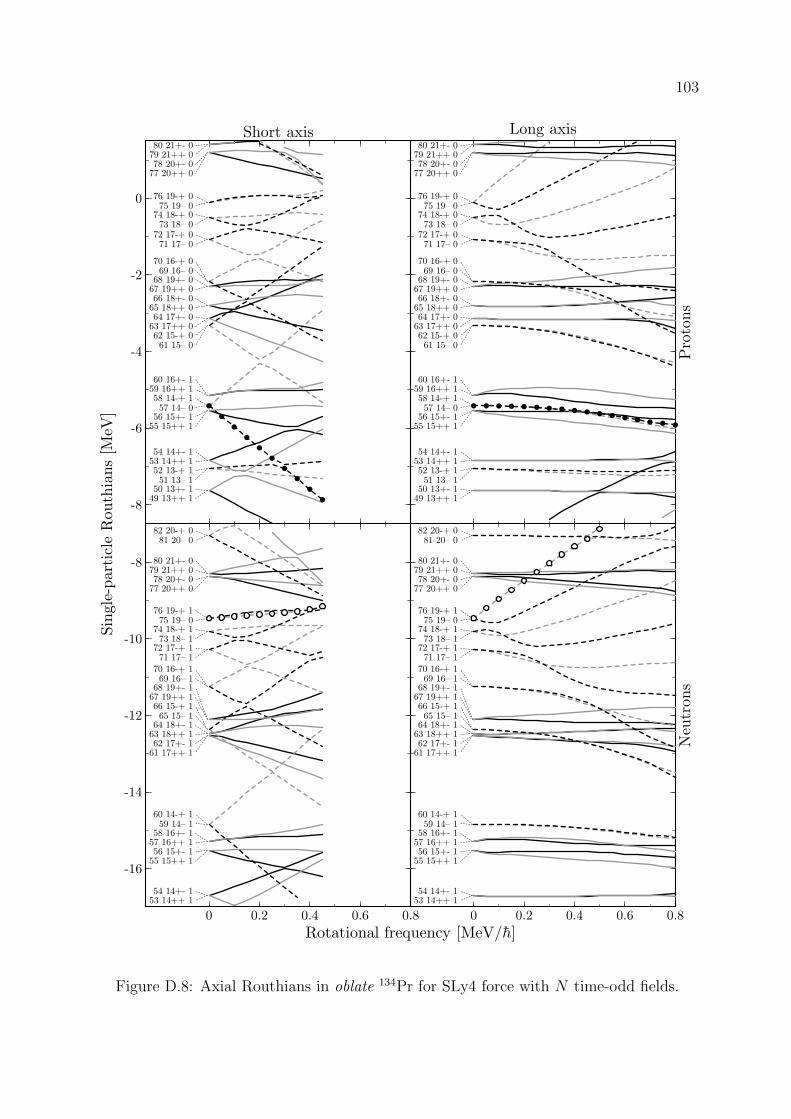
103
-8
-6
-4
-2
0
Short axis
49 13++ 150 13+- 1
51 13– 152 13-+ 1
53 14++ 154 14+- 1
55 15++ 156 15+- 1
57 14– 058 14-+ 1
59 16++ 160 16+- 1
61 15– 062 15-+ 0
63 17++ 064 17+- 0
65 18++ 066 18+- 0
67 19++ 068 19+- 0
69 16– 070 16-+ 0
71 17– 072 17-+ 0
73 18– 074 18-+ 0
75 19– 076 19-+ 0
77 20++ 078 20+- 0
79 21++ 080 21+- 0
-16
-14
-12
-10
-8
0 0.2 0.4 0.6 0.853 14++ 154 14+- 1
55 15++ 156 15+- 1
57 16++ 158 16+- 1
59 14– 160 14-+ 1
61 17++ 162 17+- 1
63 18++ 164 18+- 1
65 15– 166 15-+ 1
67 19++ 168 19+- 1
69 16– 170 16-+ 1
71 17– 172 17-+ 1
73 18– 174 18-+ 1
75 19– 076 19-+ 1
77 20++ 078 20+- 0
79 21++ 080 21+- 0
81 20– 082 20-+ 0
Pro
tons
Long axis
49 13++ 150 13+- 1
51 13– 152 13-+ 1
53 14++ 154 14+- 1
55 15++ 156 15+- 1
57 14– 058 14-+ 1
59 16++ 160 16+- 1
61 15– 062 15-+ 0
63 17++ 064 17+- 0
65 18++ 066 18+- 0
67 19++ 068 19+- 0
69 16– 070 16-+ 0
71 17– 072 17-+ 0
73 18– 074 18-+ 0
75 19– 076 19-+ 0
77 20++ 078 20+- 0
79 21++ 080 21+- 0
0 0.2 0.4 0.6 0.8
Neu
trons
53 14++ 154 14+- 1
55 15++ 156 15+- 1
57 16++ 158 16+- 1
59 14– 160 14-+ 1
61 17++ 162 17+- 1
63 18++ 164 18+- 1
65 15– 166 15-+ 1
67 19++ 168 19+- 1
69 16– 170 16-+ 1
71 17– 172 17-+ 1
73 18– 174 18-+ 1
75 19– 076 19-+ 1
77 20++ 078 20+- 0
79 21++ 080 21+- 0
81 20– 082 20-+ 0
Sin
gle
-part
icle
Routh
ians
[MeV
]
Rotational frequency [MeV/h]
Figure D.8: Axial Routhians in oblate 134Pr for SLy4 force with N time-odd fields.
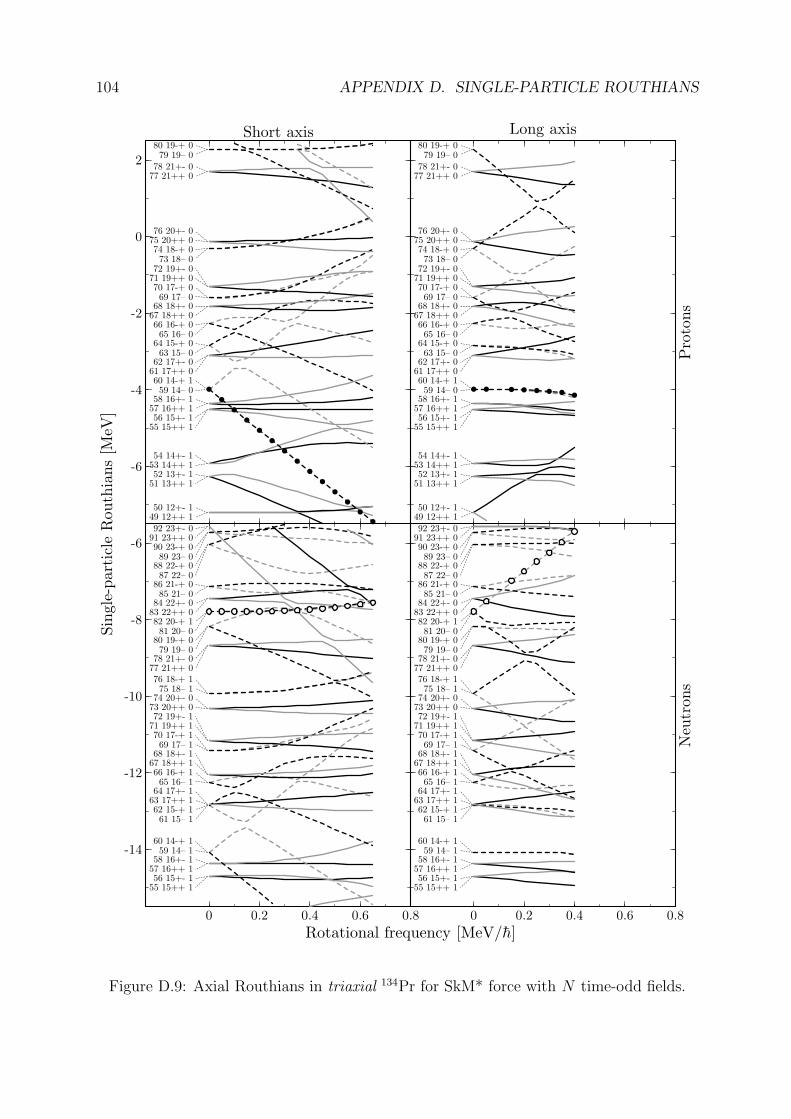
104 APPENDIX D. SINGLE-PARTICLE ROUTHIANS
-6
-4
-2
0
2
Short axis
49 12++ 150 12+- 1
51 13++ 152 13+- 1
53 14++ 154 14+- 1
55 15++ 156 15+- 1
57 16++ 158 16+- 1
59 14– 060 14-+ 1
61 17++ 062 17+- 0
63 15– 064 15-+ 0
65 16– 066 16-+ 0
67 18++ 068 18+- 0
69 17– 070 17-+ 0
71 19++ 072 19+- 0
73 18– 074 18-+ 0
75 20++ 076 20+- 0
77 21++ 078 21+- 0
79 19– 080 19-+ 0
-14
-12
-10
-8
-6
0 0.2 0.4 0.6 0.8
55 15++ 156 15+- 1
57 16++ 158 16+- 1
59 14– 160 14-+ 1
61 15– 162 15-+ 1
63 17++ 164 17+- 1
65 16– 166 16-+ 1
67 18++ 168 18+- 1
69 17– 170 17-+ 1
71 19++ 172 19+- 1
73 20++ 074 20+- 0
75 18– 176 18-+ 1
77 21++ 078 21+- 0
79 19– 080 19-+ 0
81 20– 082 20-+ 1
83 22++ 084 22+- 0
85 21– 086 21-+ 0
87 22– 088 22-+ 0
89 23– 090 23-+ 0
91 23++ 092 23+- 0
Pro
tons
Long axis
49 12++ 150 12+- 1
51 13++ 152 13+- 1
53 14++ 154 14+- 1
55 15++ 156 15+- 1
57 16++ 158 16+- 1
59 14– 060 14-+ 1
61 17++ 062 17+- 0
63 15– 064 15-+ 0
65 16– 066 16-+ 0
67 18++ 068 18+- 0
69 17– 070 17-+ 0
71 19++ 072 19+- 0
73 18– 074 18-+ 0
75 20++ 076 20+- 0
77 21++ 078 21+- 0
79 19– 080 19-+ 0
0 0.2 0.4 0.6 0.8
Neu
trons
55 15++ 156 15+- 1
57 16++ 158 16+- 1
59 14– 160 14-+ 1
61 15– 162 15-+ 1
63 17++ 164 17+- 1
65 16– 166 16-+ 1
67 18++ 168 18+- 1
69 17– 170 17-+ 1
71 19++ 172 19+- 1
73 20++ 074 20+- 0
75 18– 176 18-+ 1
77 21++ 078 21+- 0
79 19– 080 19-+ 0
81 20– 082 20-+ 1
83 22++ 084 22+- 0
85 21– 086 21-+ 0
87 22– 088 22-+ 0
89 23– 090 23-+ 0
91 23++ 092 23+- 0
Sin
gle
-part
icle
Routh
ians
[MeV
]
Rotational frequency [MeV/h]
Figure D.9: Axial Routhians in triaxial 134Pr for SkM* force with N time-odd fields.
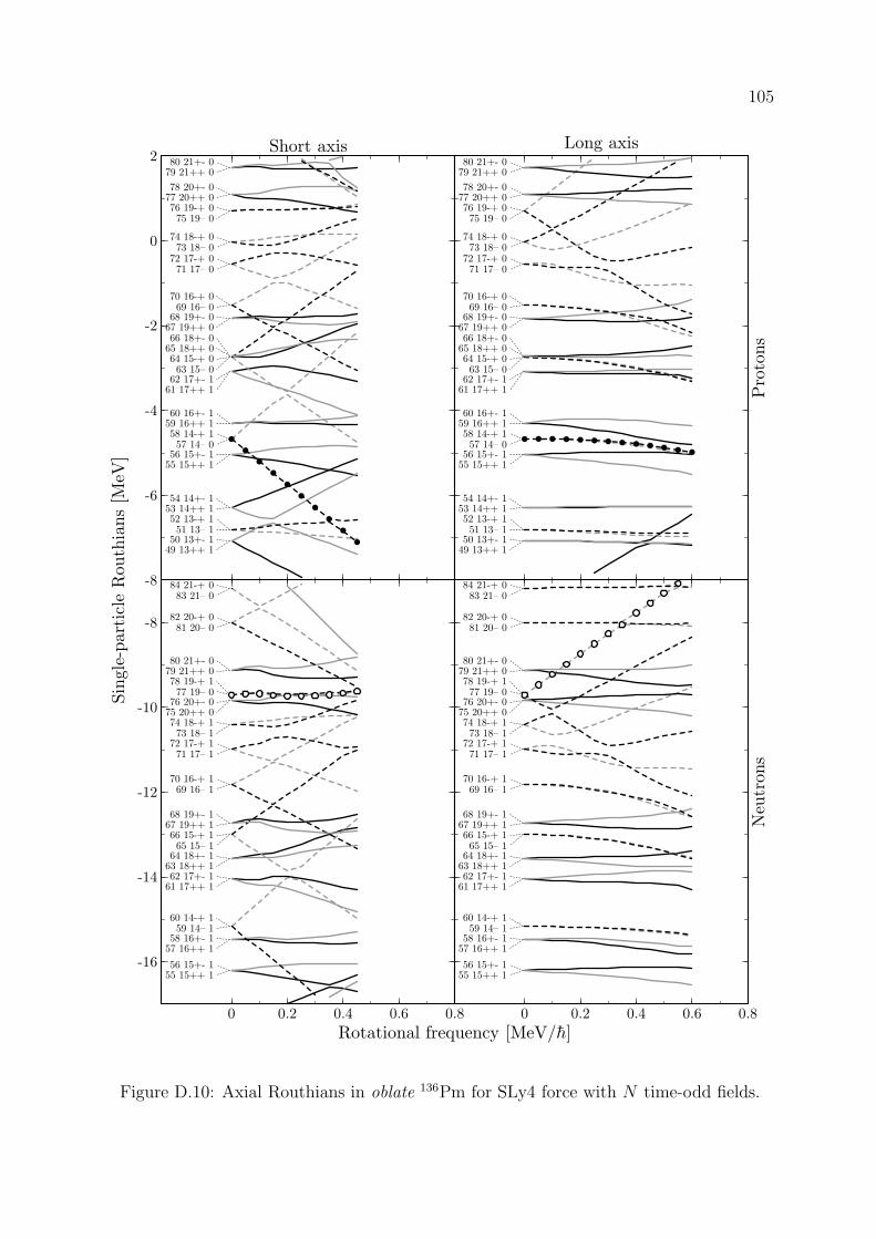
105
-8
-6
-4
-2
0
2Short axis
49 13++ 150 13+- 1
51 13– 152 13-+ 1
53 14++ 154 14+- 1
55 15++ 156 15+- 1
57 14– 058 14-+ 1
59 16++ 160 16+- 1
61 17++ 162 17+- 1
63 15– 064 15-+ 0
65 18++ 066 18+- 0
67 19++ 068 19+- 0
69 16– 070 16-+ 0
71 17– 072 17-+ 0
73 18– 074 18-+ 0
75 19– 076 19-+ 0
77 20++ 078 20+- 0
79 21++ 080 21+- 0
-16
-14
-12
-10
-8
0 0.2 0.4 0.6 0.8
55 15++ 156 15+- 1
57 16++ 158 16+- 1
59 14– 160 14-+ 1
61 17++ 162 17+- 1
63 18++ 164 18+- 1
65 15– 166 15-+ 1
67 19++ 168 19+- 1
69 16– 170 16-+ 1
71 17– 172 17-+ 1
73 18– 174 18-+ 1
75 20++ 076 20+- 0
77 19– 078 19-+ 1
79 21++ 080 21+- 0
81 20– 082 20-+ 0
83 21– 084 21-+ 0
Pro
tons
Long axis
49 13++ 150 13+- 1
51 13– 152 13-+ 1
53 14++ 154 14+- 1
55 15++ 156 15+- 1
57 14– 058 14-+ 1
59 16++ 160 16+- 1
61 17++ 162 17+- 1
63 15– 064 15-+ 0
65 18++ 066 18+- 0
67 19++ 068 19+- 0
69 16– 070 16-+ 0
71 17– 072 17-+ 0
73 18– 074 18-+ 0
75 19– 076 19-+ 0
77 20++ 078 20+- 0
79 21++ 080 21+- 0
0 0.2 0.4 0.6 0.8
Neu
trons
55 15++ 156 15+- 1
57 16++ 158 16+- 1
59 14– 160 14-+ 1
61 17++ 162 17+- 1
63 18++ 164 18+- 1
65 15– 166 15-+ 1
67 19++ 168 19+- 1
69 16– 170 16-+ 1
71 17– 172 17-+ 1
73 18– 174 18-+ 1
75 20++ 076 20+- 0
77 19– 078 19-+ 1
79 21++ 080 21+- 0
81 20– 082 20-+ 0
83 21– 084 21-+ 0
Sin
gle
-part
icle
Routh
ians
[MeV
]
Rotational frequency [MeV/h]
Figure D.10: Axial Routhians in oblate 136Pm for SLy4 force with N time-odd fields.
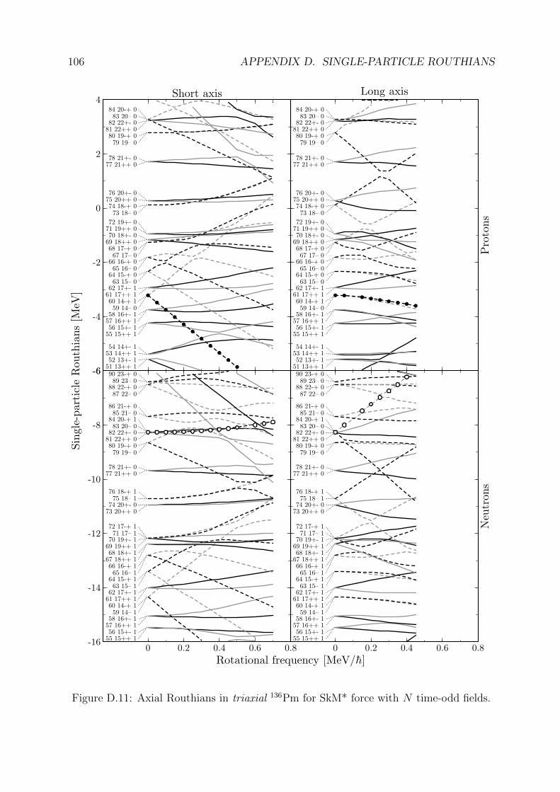
106 APPENDIX D. SINGLE-PARTICLE ROUTHIANS
-6
-4
-2
0
2
4Short axis
51 13++ 152 13+- 1
53 14++ 154 14+- 1
55 15++ 156 15+- 1
57 16++ 158 16+- 1
59 14– 060 14-+ 1
61 17++ 162 17+- 1
63 15– 064 15-+ 0
65 16– 066 16-+ 0
67 17– 068 17-+ 0
69 18++ 070 18+- 0
71 19++ 072 19+- 0
73 18– 074 18-+ 0
75 20++ 076 20+- 0
77 21++ 078 21+- 0
79 19– 080 19-+ 0
81 22++ 082 22+- 0
83 20– 084 20-+ 0
-16
-14
-12
-10
-8
-6
0 0.2 0.4 0.6 0.855 15++ 156 15+- 1
57 16++ 158 16+- 1
59 14– 160 14-+ 1
61 17++ 162 17+- 1
63 15– 164 15-+ 1
65 16– 166 16-+ 1
67 18++ 168 18+- 1
69 19++ 170 19+- 1
71 17– 172 17-+ 1
73 20++ 074 20+- 0
75 18– 176 18-+ 1
77 21++ 078 21+- 0
79 19– 080 19-+ 0
81 22++ 082 22+- 0
83 20– 084 20-+ 1
85 21– 086 21-+ 0
87 22– 088 22-+ 0
89 23– 090 23-+ 0
Pro
tons
Long axis
51 13++ 152 13+- 1
53 14++ 154 14+- 1
55 15++ 156 15+- 1
57 16++ 158 16+- 1
59 14– 060 14-+ 1
61 17++ 162 17+- 1
63 15– 064 15-+ 0
65 16– 066 16-+ 0
67 17– 068 17-+ 0
69 18++ 070 18+- 0
71 19++ 072 19+- 0
73 18– 074 18-+ 0
75 20++ 076 20+- 0
77 21++ 078 21+- 0
79 19– 080 19-+ 0
81 22++ 082 22+- 0
83 20– 084 20-+ 0
0 0.2 0.4 0.6 0.8
Neu
trons
55 15++ 156 15+- 1
57 16++ 158 16+- 1
59 14– 160 14-+ 1
61 17++ 162 17+- 1
63 15– 164 15-+ 1
65 16– 166 16-+ 1
67 18++ 168 18+- 1
69 19++ 170 19+- 1
71 17– 172 17-+ 1
73 20++ 074 20+- 0
75 18– 176 18-+ 1
77 21++ 078 21+- 0
79 19– 080 19-+ 0
81 22++ 082 22+- 0
83 20– 084 20-+ 1
85 21– 086 21-+ 0
87 22– 088 22-+ 0
89 23– 090 23-+ 0
Sin
gle
-part
icle
Routh
ians
[MeV
]
Rotational frequency [MeV/h]
Figure D.11: Axial Routhians in triaxial 136Pm for SkM* force with N time-odd fields.
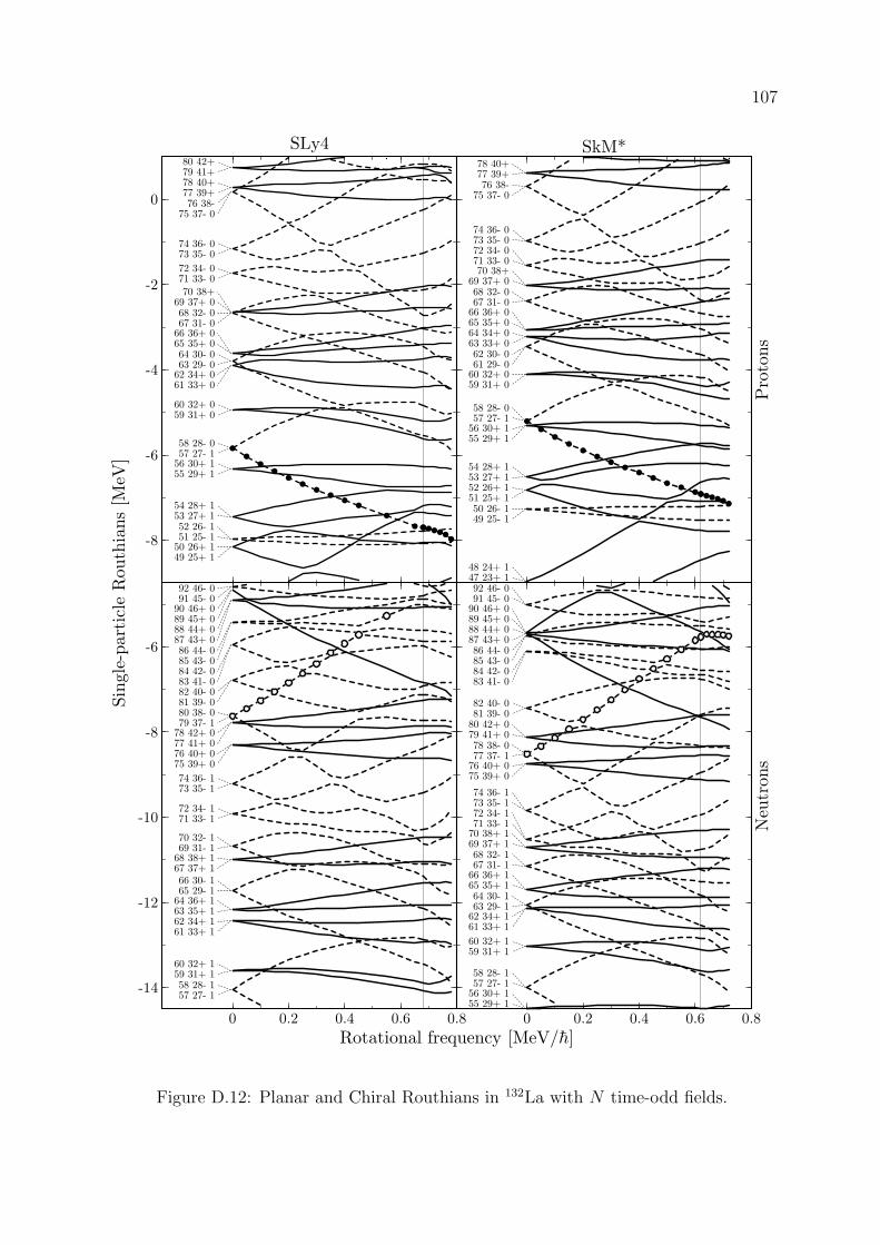
107
-8
-6
-4
-2
0
SLy4
49 25+ 150 26+ 151 25- 152 26- 1
53 27+ 154 28+ 1
55 29+ 156 30+ 157 27- 158 28- 0
59 31+ 060 32+ 0
61 33+ 062 34+ 063 29- 064 30- 0
65 35+ 066 36+ 067 31- 068 32- 0
69 37+ 070 38+
71 33- 072 34- 0
73 35- 074 36- 0
75 37- 076 38-
77 39+78 40+79 41+80 42+
-14
-12
-10
-8
-6
0 0.2 0.4 0.6 0.8
57 27- 158 28- 1
59 31+ 160 32+ 1
61 33+ 162 34+ 163 35+ 164 36+ 165 29- 166 30- 1
67 37+ 168 38+ 169 31- 170 32- 1
71 33- 172 34- 1
73 35- 174 36- 1
75 39+ 076 40+ 077 41+ 078 42+ 079 37- 180 38- 081 39- 082 40- 083 41- 084 42- 085 43- 086 44- 0
87 43+ 088 44+ 089 45+ 090 46+ 091 45- 092 46- 0
Pro
tons
SkM*
47 23+ 148 24+ 1
49 25- 150 26- 1
51 25+ 152 26+ 153 27+ 154 28+ 1
55 29+ 156 30+ 157 27- 158 28- 0
59 31+ 060 32+ 061 29- 062 30- 0
63 33+ 064 34+ 065 35+ 066 36+ 067 31- 068 32- 0
69 37+ 070 38+
71 33- 072 34- 073 35- 074 36- 0
75 37- 076 38-
77 39+78 40+
0 0.2 0.4 0.6 0.8
Neu
trons
55 29+ 156 30+ 157 27- 158 28- 1
59 31+ 160 32+ 1
61 33+ 162 34+ 163 29- 164 30- 1
65 35+ 166 36+ 167 31- 168 32- 1
69 37+ 170 38+ 171 33- 172 34- 173 35- 174 36- 1
75 39+ 076 40+ 077 37- 178 38- 0
79 41+ 080 42+ 081 39- 082 40- 0
83 41- 084 42- 085 43- 086 44- 0
87 43+ 088 44+ 089 45+ 090 46+ 091 45- 092 46- 0
Sin
gle
-part
icle
Routh
ians
[MeV
]
Rotational frequency [MeV/h]
Figure D.12: Planar and Chiral Routhians in 132La with N time-odd fields.
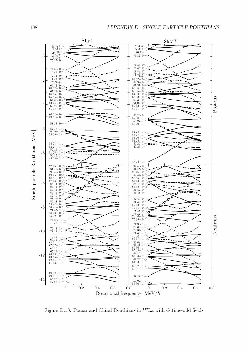
108 APPENDIX D. SINGLE-PARTICLE ROUTHIANS
-8
-6
-4
-2
0
SLy4
49 25+ 150 25- 1
51 26+ 152 26- 1
53 27+ 154 28+ 1
55 29+ 156 30+ 157 27- 1
58 28- 0
59 31+ 060 32+ 0
61 33+ 062 29- 0
63 34+ 064 30- 0
65 35+ 066 36+ 067 31- 0
68 37+ 069 32- 070 38+
71 33- 072 34- 0
73 35- 074 36- 0
75 37- 076 39+77 40+78 38-
79 41+80 42+
-14
-12
-10
-8
-6
0 0.2 0.4 0.6 0.8
57 27- 158 28- 1
59 31+ 160 32+ 1
61 33+ 162 34+ 163 35+ 164 36+ 165 29- 166 30- 1
67 37+ 168 38+ 169 31- 170 32- 1
71 33- 172 34- 1
73 35- 174 36- 1
75 39+ 076 40+ 077 37- 1
78 41+ 079 42+ 080 38- 081 39- 082 40- 083 41- 084 42- 085 43- 086 44- 0
87 43+ 088 44+ 089 45+ 090 45- 091 46- 0
92 46+ 0
Pro
tons
SkM*
48 24+ 1
49 25- 150 26- 1
51 25+ 152 26+ 153 27+ 154 28+ 1
55 29+ 156 27- 1
57 30+ 158 28- 0
59 31+ 060 32+ 061 29- 062 30- 0
63 33+ 064 34+ 065 35+ 066 36+ 067 31- 068 32- 0
69 37+ 070 38+
71 33- 072 34- 073 35- 074 36- 0
75 37- 076 38-
77 39+78 40+
0 0.2 0.4 0.6 0.8
Neu
trons
56 30+ 157 27- 1
58 28- 1
59 31+ 160 32+ 1
61 33+ 162 29- 1
63 34+ 164 30- 1
65 35+ 166 36+ 167 31- 168 32- 1
69 37+ 170 38+ 171 33- 172 34- 173 35- 174 36- 1
75 39+ 076 40+ 077 37- 178 38- 0
79 41+ 080 42+ 081 39- 082 40- 0
83 41- 084 42- 0
85 43+ 086 43- 0
87 44+ 088 45+ 089 44- 0
90 46+ 091 45- 092 46- 0
Sin
gle
-part
icle
Routh
ians
[MeV
]
Rotational frequency [MeV/h]
Figure D.13: Planar and Chiral Routhians in 132La with G time-odd fields.
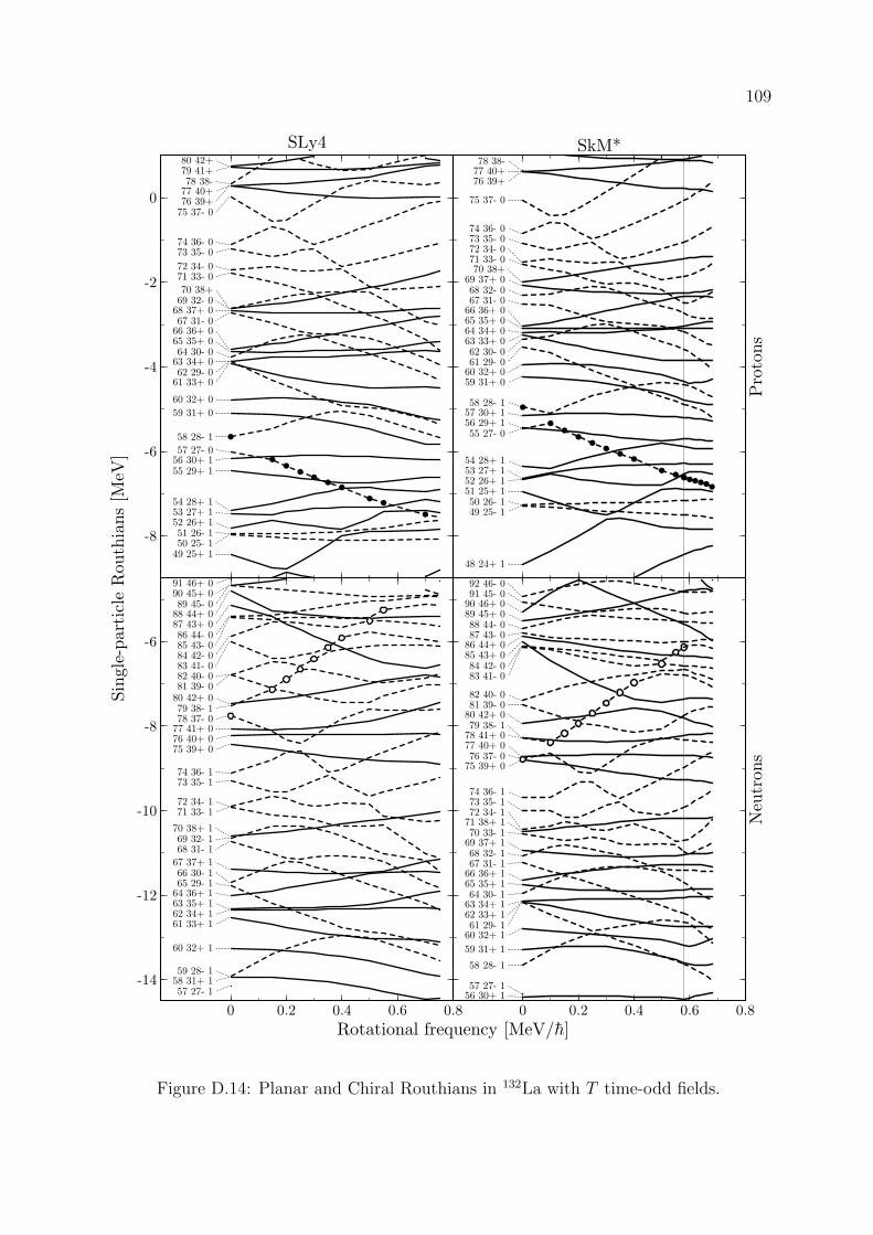
109
-8
-6
-4
-2
0
SLy4
49 25+ 150 25- 151 26- 1
52 26+ 153 27+ 154 28+ 1
55 29+ 156 30+ 157 27- 0
58 28- 1
59 31+ 0
60 32+ 0
61 33+ 062 29- 0
63 34+ 064 30- 0
65 35+ 066 36+ 067 31- 0
68 37+ 069 32- 070 38+
71 33- 072 34- 0
73 35- 074 36- 0
75 37- 076 39+77 40+78 38-
79 41+80 42+
-14
-12
-10
-8
-6
0 0.2 0.4 0.6 0.8
57 27- 158 31+ 159 28- 1
60 32+ 1
61 33+ 162 34+ 163 35+ 164 36+ 165 29- 166 30- 1
67 37+ 1
68 31- 169 32- 1
70 38+ 1
71 33- 172 34- 1
73 35- 174 36- 1
75 39+ 076 40+ 077 41+ 078 37- 079 38- 1
80 42+ 081 39- 082 40- 083 41- 084 42- 085 43- 086 44- 0
87 43+ 088 44+ 089 45- 0
90 45+ 091 46+ 0
Pro
tons
SkM*
48 24+ 1
49 25- 150 26- 1
51 25+ 152 26+ 153 27+ 154 28+ 1
55 27- 056 29+ 157 30+ 158 28- 1
59 31+ 060 32+ 061 29- 062 30- 0
63 33+ 064 34+ 065 35+ 066 36+ 067 31- 068 32- 0
69 37+ 070 38+
71 33- 072 34- 073 35- 074 36- 0
75 37- 0
76 39+77 40+78 38-
0 0.2 0.4 0.6 0.8
Neu
trons
56 30+ 157 27- 1
58 28- 1
59 31+ 1
60 32+ 161 29- 1
62 33+ 163 34+ 164 30- 1
65 35+ 166 36+ 167 31- 168 32- 1
69 37+ 170 33- 1
71 38+ 172 34- 173 35- 174 36- 1
75 39+ 076 37- 0
77 40+ 078 41+ 079 38- 1
80 42+ 081 39- 082 40- 0
83 41- 084 42- 0
85 43+ 086 44+ 087 43- 088 44- 0
89 45+ 090 46+ 091 45- 092 46- 0
Sin
gle
-part
icle
Routh
ians
[MeV
]
Rotational frequency [MeV/h]
Figure D.14: Planar and Chiral Routhians in 132La with T time-odd fields.

110 APPENDIX D. SINGLE-PARTICLE ROUTHIANS
Bibliography
[Abo92a] Y. Aboussir et al., Nucl. Phys. A549, 155 (1992)
[Ami01a] Amita, A.K. Jain, B. Singh, Table of magnetic dipole rotational bands(www.nndc.bnl.gov, 2001)
[Ant02a] M.S. Antony, Nuclide Chart 2002 (Strasbourg, 2002)
[Bal92a] G. Baldsiefen et al., Phys. Lett. B275, 252 (1992)
[Bal94a] G. Baldsiefen et al., Nucl. Phys. A574, 521 (1994)
[Bar82a] J. Bartel et al., Nucl. Phys. A386, 79 (1982)
[Bar01a] R.A. Bark et al., Nucl. Phys. A691, 577 (2001)
[Bea01a] C.W. Beausang et al., Nucl. Phys. A682, 394c (2001)
[Ben02a] M. Bender et al., Phys. Rev. C65, 054322 (2002)
[Boh53a] A. Bohr, B.R. Mottelson, Mat. Fys. Medd. Kong. Dansk. Vid. Selsk. 27, No.16 (1953)
[Boh75a] A. Bohr, B.R. Mottelson, Nuclear Structure (Benjamin, New York, 1975)
[Boh80a] A. Bohr, B.R. Mottelson, Phys. Scripta 22, 461 (1980)
[Cha97a] E. Chabanat et al., Nucl. Phys. A627, 710 (1997)
[Chm97a] S. Chmel et al., Phys. Rev. Lett. 79, 2002 (1997)
[Cla92a] R.M. Clark et al., Phys. Lett. B275, 247 (1992)
[Cla00a] R.M. Clark, A.O. Macchiavelli, Annu. Rev. Nucl. Part. Sci. 50, 1 (2000)
[Dav58a] A.S. Davydov, B.F. Fillipov, Nucl. Phys. 8, 237 (1958)
[Dim00a] V.I. Dimitrov, S. Frauendorf, F. Donau, Phys. Rev. Lett. 84, 5732 (2000)
[Dim00b] V.I. Dimitrov, F. Donau, S. Frauendorf, Phys. Rev. C62, 24315 (2000)
[Dim02a] V.I. Dimitrov, F. Donau, S. Frauendorf, nucl-th/0211063v1 (2002)
[Dob84a] J. Dobaczewski, H. Flocard, J. Treiner, Nucl. Phys. A422, 103 (1984)
111
112 BIBLIOGRAPHY
[Dob87a] J. Dobaczewski, Wybrane zagadnienia teorii jadra atomowego (skrypt dowyk ladu) (1987)
[Dob95a] J. Dobaczewski, J. Dudek, Phys. Rev. C52, 1827 (1995)
[Dob97a] J. Dobaczewski, J. Dudek, Phys. Rev. C55, 3177(E) (1997)
[Dob00a] J. Dobaczewski, J. Dudek, Comp. Phys. Comm. 102, 166 (1997); 102, 183(1997); 131, 164 (2000)
[Dob00b] J. Dobaczewski et al., Phys. Rev. C62, 014310 (2000); C62, 014311 (2000)
[Dob04a] J. Dobaczewski, P. Olbratowski, Comp. Phys. Comm. 158, 158 (2004)
[Dud04a] J. Dudek, N. Schunck, private communication (2004)
[Eng75a] Y.M. Engel et al., Nucle. Phys. A249, 215 (1975)
[Eng03a] J. Engel et al., Phys. Rev. C68, 025501 (2003)
[Fra91a] S. Frauendorf, T. Bengtsson, AIP Conf. Proc. 259, 223 (1991)
[Fra92a] S. Frauendorf, F.R. May, Proc. of the Int. Conf. on Nuclear Structure at HighAngular Momentum (Ottawa, 1992)
[Fra93a] S. Frauendorf, Nucl. Phys. A557, 259c (1993)
[Fra96a] S. Frauendorf, J. Reif, G. Winter, Nucl. Phys. A601, 41 (1996)
[Fra96b] S. Frauendorf, J. Meng, Zeit. fur Phys. A356, 263 (1996)
[Fra97a] S. Frauendorf, J. Meng, Nucl. Phys. A617, 131 (1997)
[Fra97b] S. Frauendorf, J. Reif, Nucl. Phys. A621, 736 (1997)
[Fra97c] S. Frauendorf, Zeit. fur Phys. A358, 163 (1997)
[Fra00a] S. Frauendorf, Nucl. Phys. A677, 115 (2000)
[Fra01a] S. Frauendorf, Rev. Mod. Phys. 73, 463 (2001)
[Fra01b] S. Frauendorf, Acta Phys. Pol. 32, 2661 (2001)
[Fra03a] S. Frauendorf, private communication (2003)
[Fri87a] H. Frisk, R. Bengtsson, Phys. Lett. B196, 14 (1987)
[Gol53a] H. Goldstein, Classical Mechanics (Addison-Wesley, Cambridge, 1953)
[Gro04a] E. Grodner et al., Int. Journ. of Mod. Phys. E13, 243 (2004)
[Gro04b] E. Grodner, J. Srebrny, private communication (2004)
[Har01a] D.J. Hartley et al., Phys. Rev. C64, 31304 (2001)
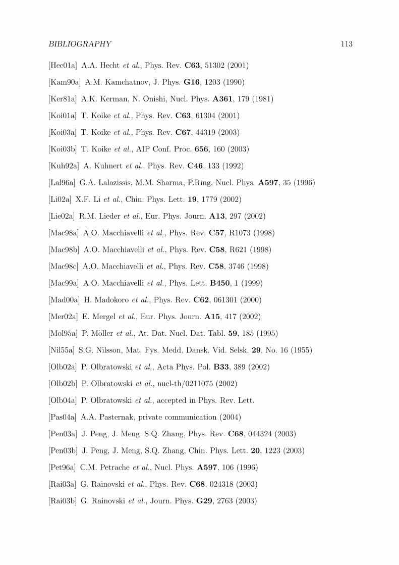
BIBLIOGRAPHY 113
[Hec01a] A.A. Hecht et al., Phys. Rev. C63, 51302 (2001)
[Kam90a] A.M. Kamchatnov, J. Phys. G16, 1203 (1990)
[Ker81a] A.K. Kerman, N. Onishi, Nucl. Phys. A361, 179 (1981)
[Koi01a] T. Koike et al., Phys. Rev. C63, 61304 (2001)
[Koi03a] T. Koike et al., Phys. Rev. C67, 44319 (2003)
[Koi03b] T. Koike et al., AIP Conf. Proc. 656, 160 (2003)
[Kuh92a] A. Kuhnert et al., Phys. Rev. C46, 133 (1992)
[Lal96a] G.A. Lalazissis, M.M. Sharma, P.Ring, Nucl. Phys. A597, 35 (1996)
[Li02a] X.F. Li et al., Chin. Phys. Lett. 19, 1779 (2002)
[Lie02a] R.M. Lieder et al., Eur. Phys. Journ. A13, 297 (2002)
[Mac98a] A.O. Macchiavelli et al., Phys. Rev. C57, R1073 (1998)
[Mac98b] A.O. Macchiavelli et al., Phys. Rev. C58, R621 (1998)
[Mac98c] A.O. Macchiavelli et al., Phys. Rev. C58, 3746 (1998)
[Mac99a] A.O. Macchiavelli et al., Phys. Lett. B450, 1 (1999)
[Mad00a] H. Madokoro et al., Phys. Rev. C62, 061301 (2000)
[Mer02a] E. Mergel et al., Eur. Phys. Journ. A15, 417 (2002)
[Mol95a] P. Moller et al., At. Dat. Nucl. Dat. Tabl. 59, 185 (1995)
[Nil55a] S.G. Nilsson, Mat. Fys. Medd. Dansk. Vid. Selsk. 29, No. 16 (1955)
[Olb02a] P. Olbratowski et al., Acta Phys. Pol. B33, 389 (2002)
[Olb02b] P. Olbratowski et al., nucl-th/0211075 (2002)
[Olb04a] P. Olbratowski et al., accepted in Phys. Rev. Lett.
[Pas04a] A.A. Pasternak, private communication (2004)
[Pen03a] J. Peng, J. Meng, S.Q. Zhang, Phys. Rev. C68, 044324 (2003)
[Pen03b] J. Peng, J. Meng, S.Q. Zhang, Chin. Phys. Lett. 20, 1223 (2003)
[Pet96a] C.M. Petrache et al., Nucl. Phys. A597, 106 (1996)
[Rai03a] G. Rainovski et al., Phys. Rev. C68, 024318 (2003)
[Rai03b] G. Rainovski et al., Journ. Phys. G29, 2763 (2003)
114 BIBLIOGRAPHY
[Rei95a] P.G. Reinhard, H. Flocard, Nucl. Phys. A584, 467 (1995)
[Rie60a] B. Riemann, Abh. Kon. Ges. Wiss. 9, 1 (1860)
[Rin00a] P. Ring, P. Schuck, The Nuclear Many-Body Problem (Springer, Berlin, 2000)
[Rob03a] S.P. Roberts et al., Phys. Rev. C67, 057301 (2003)
[Rza01a] T. Rzaca-Urban, Acta Phys. Pol. B32, 2645 (2001)
[Sat94a] W. Satu la, R. Wyss, Phys. Rev. C50, 2888 (1994)
[Sta88a] W. Starzecki et al., Phys. Lett. B200, 419 (1988)
[Sta01a] K. Starosta et al., Nucl. Phys. A682, 375c (2001)
[Sta01b] K. Starosta et al., Phys. Rev. Lett. 86, 971 (2001)
[Sta02a] K. Starosta et al., Phys. Rev. C65, 044328 (2002)
[Sta03a] K. Starosta, P. Joshi, private communication
[Sug97a] M. Sugawara et al., Zeit. fur Phys. A358, 1 (1997)
[Tho62a] D.J. Thouless, J.G. Valatin, Nucl. Phys. 31, 211 (1962)
[Tim03a] J. Timar et al., Eur. Journ. of Phys. A16, 1 (2003)
[Uma91a] A.S. Umar et al., Phys. Rev. C44, 2512 (1991)
[Vam04a] C. Vaman et al., Phys. Rev. Lett. 92, 032501 (2004)
[Vol98a] V. Volterra, Acta Mathematica 22, 201 (1898)
[Woo54a] R.D. Woods, D.S. Saxon, Phys. Rev. 95, 577 (1954)
[Yam00a] M. Yamagami, K. Matsuyanagi, Nucl. Phys. A672, 123 (2000)
[Yam01a] M. Yamagami, K. Matsuyanagi, M. Matsuo, Nucl. Phys. A693, 579 (2001)
[Zhu03a] S. Zhu et al., Phys. Rev. Lett. 91, 132501 (2003)


![Oddzia Kliniczny Radioterapii · NCRP 151 [12] oraz parametrów, uwzględniając specyfikację pracy Oddziału Klinicznego Radioterapii. Jednostka organizacyjna powinna zweryfikować](https://img.pdfslide.tips/doc/110x75/606091f1469f3957784e5d10/oddzia-kliniczny-radioterapii-ncrp-151-12-oraz-parametrw-uwzgldniajc-specyfikacj.jpg)