Embed Size (px)
Citation preview

Land, water andLand, water and ecosystem nexus forecosystem nexus for
climate risk managementclimate risk managementYoshiki Yamagata, Tokuta YokohataNational Institute for Environmental Studies
Akihiko Ito, Naota Hanasaki, Etsushi Kato (NIES), , , ( ),Kazuya Nishina, Yoshimitsu Masaki (NIES),
Tsuguki Kinoshita, Motoko Inatomi (Ibaraki Univ), k h h k ( )Gen Sakurai, Toshichika Iizumi (NIAES),
Masashi Okada, Motoki Nishimori (NIAES)
6th Dec 2013, ICA‐RUS workshop

ContentsContentsk d d bj i• Background, scope and objective
– Land‐Water‐Ecosystem “nexus” approachLand Water Ecosystem nexus approach
• Status and key findings– Land: Land use change, down scalingWater: Future water scenario water scarcity–Water: Future water scenario, water scarcity
– Ecosystem: Model uncertainty, global crop yield
• Challenges for the future

Land, water, ecosystem “nexus”• Land
A basis for human life (agricultural/urban area) and– A basis for human life (agricultural/urban area) and ecosystem (forest etc)
– Land use change affects/controls climate changeLand use change affects/controls climate change
• WaterU d f f d ( i lt t ) d h lif– Used for food (agriculture etc), energy, and human life
– Water resources is affected by climate change
E t• Ecosystem– Provides food (agriculture etc) as well as energy (bio crop)– Ecosystem (vegetation etc) affects/controls climate change
“Nexus approach” (trans‐sectoral multi‐scales) isNexus approach (trans‐sectoral, multi‐scales) is essential for climate risk management

Our “nexus” approachIntegration (sub‐1) Y. Yamagata, T. Yokohata, E. Kato (NIES) Synergy/trade‐off analysis, Urban growth + Downscaling techniquey gy/ y , g g q
Crop calendar・RunoffFloodplain area Water resouces (sub‐3)
N. Hanasaki (NIES)Eco‐system (sub‐2)
A. Ito (NIES)Vegetation・LAI
N. Hanasaki (NIES)Operation of reservoirs
Sustainability of water use
( )Forest management
Sustainability of eco‐system services
Land useFertilizer
Agriculturalecosystem
Forest/Grasslandproductivity
Land use
Crop calendarIrrigation Irrigation
demand
Land use・Fertilizer
Land use
Agriculture (sub‐5)M. Nishimori (NIAES)
Land use (sub‐4)T. Kinoshita (U. Ibaraki)
Crop productivity
( )Sustainability of crop
productivity
( )Crop management
Sustainability of land use
Model input: Socio‐economic scenario (RCP, SSP etc.), climate scenario (CMIP4/5)Population, GDP, future “story‐line”, changes in climate (temperature, precipitation etc)

Objectivesj• Low‐carbon scenario?
– Sustainability of intensive mitigation/adaptation options, such as negative emission?
– Potential of future Bio‐Energy Carbon Capture and Storage (BECCS) and 2 degree target: by E. KatoStorage (BECCS) and 2 degree target: by E. Kato
• Business as usual (high‐carbon) scenario?– Interaction between land, water, ecosystem?– “Climate Boundary”: how resilient are we?
• Development of models and data‐basesCoupling of land water ecosystem models– Coupling of land‐water‐ecosystem models

Development of “Integrated terrestrial model”Socio‐economic + Climate scenarioGDP, population, Temperature, precipitation, ..
Erosion
Water resourcesWater use by human activity (agriculture,
Afforestation/deforestation
Eco‐systemThe exchange of C and NCO2 emissions
Water use(Agriculture etc )
ac y (ag cu u e,industry) is estimated. Irrigation from river is considered.
between atmosphere‐vegetation‐soil is calculated. Changes in
from land use
Greenhouse gasbudget
(Agriculture, etc.)
Crop productivity Fertilizeri t GHG are estimated. budgetCO2 emissions
from forest fire
A i l
input
L d( )AgricultureCrop productivity is estimated . The production
Land useLand‐use change (cropland‐forest) is calculated based on future socio‐
i i E i
Land(MATSIRO)& Climate(MIROC)
Soil water, temperature areof bio‐energy crop for mitigation option is considered.
economic scenarios. Economic (e.g., trade) +natural (e.g. inclination) factors are considered.
Soil water, temperature are calculated based on the water‐energy budget.

L dLandModelling of land use changeModelling of land use change,
Development of down scaling method

Spatially explicit urban growth modelSpatial interactionsLatest urban modeling
Spatial Econometrics
Socio‐economic scenarios
RCP StrongNeo Economic Geography (NEG)SSP
Develop new Urban Growth modelsValidationConduct Simulations
Input dataAlgorithm developmentU b th d l
Test Urban GIS statisticsSatellite R/S dataConduct Simulations
Checking with dataFeedbackUrban growth model using R/S and GIS data
Spatial autocorrelation
Satellite R/S data(MODIS, DMSP etc.)
Spatial autocorrelationEconomic agglomeration
Feedback
Population, GDP: Country Population, GDP:50km grid
Downscale urban growth with bottom up modeling

Creation of future gridded population and GDP of the world
Rank-size rule based
Gravity model based

Database for gridded populationDatabase for gridded population
Tatem, A. J., Campiz, N., Gething, P. W., Snow, R. W., & Linard, C. (2011). The effects of spatial population dataset choice on estimates of population at risk of disease. Population health metrics, 9(1), 4.
Population Count Grid v3(PCGv3)by SEDAC is freely available, and most widely used.is freely available, and most widely used.

Problem of SEDAC population database
Mesh block size is about 4 km x 4kmMesh block size is about 4 km x 4km
Saudi Arabia 2000Saudi Arabia, 2000
Creating using areal weighting, and overly smoothed.Fi t f ll h t i d t b ild ti l t ti ti l
11
First of all, we have tried to build a spatial statistical model to refine this data set.
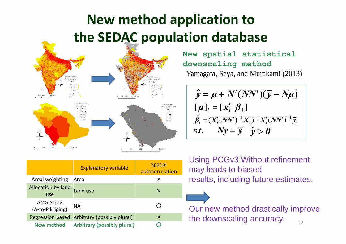
New method application to the SEDAC population database
New spatial statisticaldownscaling method
the SEDAC population database
))((ˆ NμyNNNμy
gYamagata, Seya, and Murakami (2013)
iiiii yNNXXNNXβ 111 )())((ˆ
))(( NμyNNNμy ][][ iii xμ
iiiii yNNXXNNXβ )())((
0y ˆyNy ..ts
Using PCGv3 Without refinement may leads to biased
lt i l di f t ti tExplanatory variable Spatial
autocorrelationl i h i results, including future estimates.Areal weighting Area ×
Allocation by land use Land use ×
ArcGIS10.2 NA ○
12
Our new method drastically improvethe downscaling accuracy.
(A‐to‐P kriging) NA ○
Regression based Arbitrary (possibly plural) ×
New method Arbitrary (possibly plural) ○

Land use model: Constraint by yield, inclination
0 80
0.90
1.00
]
Cropland with inclination > 0.3 deg (USA) Cropland and inclination(Italy)
0.40
0.50
0.60
0.70
0.80
urb
an/cro
plan
d [-
]
op ra
tio
op ra
tio
0.00
0.10
0.20
0.30
1 8
15
22
29
36
43
50
57
64
71
78
85
92
99
rati
o o
f u
Cro
Cro
2 2 3 4 5 5 6 7 7 8 9 9
Cropland in Australia Cropland in CanadaCropland in Australia Cropland in Canada
Yield [tons/ha] Inclination [0.1 degree]
15000000
20000000
25000000
50
60
70
80
90
15000000
20000000
25000000
40
50
60
70
p C op a d Ca ada
0
5000000
10000000
0
10
20
30
40
0
5000000
10000000
0
10
20
30
ModelObserved
ModelObserved
人口分布1970 1975 1980 1985 1990 1995 2000 2005 1970 1975 1980 1985 1990 1995 2000 20051970 1980 1990 2000 20051970 1980 1990 2000 2005

Land, water andLand, water and ecosystem nexus forecosystem nexus for
climate risk managementclimate risk managementYoshiki Yamagata, Tokuta Yokohata
National Institute for Environmental Studies
Akihiko Ito, Naota Hanasaki, Etsushi Kato (NIES), , , ( ),Kazuya Nishina, Yoshimitsu Masaki (NIES),
Tsuguki Kinoshita, Motoko Inatomi (Ibaraki Univ), k h h k ( )Gen Sakurai, Toshichika Iizumi (NIAES),
Masashi Okada, Motoki Nishimori (NIAES)
6th Dec 2013, ICA‐RUS workshop

WaterWaterFuture scenario of water useFuture scenario of water use,
water scarcity

Global water scarcity assessmentGlobal hydrological model with human activities
SSP: Shared Socioeconomic Pathways• SSP is a global socio‐economic scenario, the
successor of SRES Five different views of the
We also developed a scenario matrix of SSP and RCP.We analyzed the results
h/ h l lsuccessor of SRES. Five different views of the world are depicted.
• SSP doesn’t include scenarios on water. We developed a compatible water use scenario.
with/without climate policy.
p p
Hanasaki et al. 2013a,b, Hydrology and Earth System Sciences

2041‐2070, difference from presentSSP1 li ith li t li
Global water scarcity assessment
Water resources assessment• Water availability and use was
simulated at daily interval, at spatial
SSP1 no policy with climate policy
simulated at daily interval, at spatial resolution of 0.5 deg x 0.5 deg.
• A new index for water scarcity was d t l t h th t i
SSP2 no policy with climate policy
used to evaluate whether water is available when it is needed. SSP3 no policy with climate policy
Water stressed populationclimatepolicy
SSP4 no policy with climate policyp y
SSP5 no policy with climate policy
Water stressed population, RED=worse
Hanasaki et al. 2013a,b, Hydrology and Earth System Sciences
• Ten sets of comprehensive global water scenarios have been developed.p p ,

2041‐2070, difference from presentSSP1 li ith li t li
Global water scarcity assessmentB t iWater resources assessment
• Water availability and use was simulated at daily interval, at spatial
SSP1 no policy with climate policyBest scenario‐Sustainable society‐Efficient climate policy‐Water stress stabilizes except Africasimulated at daily interval, at spatial resolution of 0.5 deg x 0.5 deg.
• A new index for water scarcity was d t l t h th t i
SSP2 no policy with climate policyBAU scenario‐Middle of the road
p
used to evaluate whether water is available when it is needed. SSP3 no policy with climate policy
‐Moderate climate policy‐Water stress increases (stressed population doubles at the end of 21C)
Water stressed populationSSP4 no policy with climate policy
Worst scenario
SSP5 no policy with climate policy
‐Low technological change and low environmental consciousness‐ High birth rate and low income‐Water stress heavily increases (stressed
Water stressed population, RED=worse
‐Water stress heavily increases (stressed population triples at the end of 21C)
Hanasaki et al. 2013a,b, Hydrology and Earth System Sciences
• Ten sets of comprehensive global water scenarios have been developed.p p ,

EcosystemEcosystemGlobal crop yield and climate changep y gUncertainty in ecosystem models

Dataset of historical changes in global yields
By combining global agricultural datasets
Global Dataset of
agricultural datasetsrelated to crop calendar andGlobal Dataset of
Historical Yieldscalendar and
harvested area in 2000 country yield2000, country yield
statistics, and satellite derived net
Iizumi et al (2013) Glob Ecol & Biogeogr
satellite‐derived net primary production
During 1982‐2006 with a resolution of 1.125o × 1.125o
Iizumi et al. (2013) Glob Ecol & Biogeogr
gMaize, soybean, rice, and wheat.

Dominant climatic factorsaffecting year to year variations in the yieldaffecting year‐to‐year variations in the yield
δYieldt=a1ΔTt+a2ΔWt+ε
Temperature
1 t 2 t
Soil moisture
Iizumi et al. (2013) Nature Climate Change
Dominant factors (temperature , soil moisture) are different among crops and regions.
Climatic constrains ‐> Future climate change impacts

Improved Process‐based Regional‐scale crop Yield Simulator with Bayesian Inference (PRYSBI2)Simulator with Bayesian Inference (PRYSBI2)
Global yieldGlobal yield of maize in 2001(Iizumi et al 2013)(Iizumi et al 2013)
Estimated yieldEstimated yield of maize in 2001By PRISBI2By PRISBI2Calibrated by Even‐numbered years
Process‐based, regional‐scale crop modelg p Predictability for global scale (maize, soybean, rice, wheat)

Uncertainty in terrestrial ecosystem models
Contribution to“ISI MIP”
Biomass increase
ISI‐MIP analysis on carbon response
“ISI‐MIP”: Inter‐sector Impact Model Inter‐comparison Project
Uncertainty
T h [K]
Impact assessment byHot spots [areas] in carbon change
Temp. change [K]
p y4 RCPs
x 5 climate modelsUncertainties in socio‐economic and climate scenario
Friend et al. 2013, in press, PNAS

Uncertainty in terrestrial ecosystem modelsISI‐MIP analysis on soil carbon response
high
low
R f ilResponse of soil carbon to temperature change differs among models.
Nishina et al. (submitted to Earth System Dynamics)

FutureFuturechallengesgCoupling of land‐water‐Coupling of land water
ecosystem modelsFuture risks under climate change

Nexus approach by “Integrated terrestrial model”Socio‐economic + Climate scenarioGDP, population, Temperature, precipitation, ..
Erosion
Water resourcesWater use by human activity (agriculture,
Afforestation/deforestation
Eco‐systemThe exchange of C and NCO2 emissions
Water use(Agriculture etc )
ac y (ag cu u e,industry) is estimated. Irrigation from river is considered.
between atmosphere‐vegetation‐soil is calculated. Changes in
from land use
Greenhouse gasbudget
(Agriculture, etc.)
Crop productivityFertilizeri t GHG are estimated. budgetCO2 emissions
from forest fire
A i l
C op p oduc y input
L dAgricultureCrop productivity is estimated . The production
Land useLand‐use change (cropland‐forest) is calculated based on future socio‐
i i E i
Land& ClimateSoil water, temperature are calculated based on the
of bio‐energy crop for mitigation option is considered.
economic scenarios. Economic (e.g., trade) +natural (e.g. inclination) factors are considered.
water and energy budget. Atmospheric processes
(precipitation etc) is option.

Nexus approach by “Integrated terrestrial model”Socio‐economic + Climate scenarioGDP, population, Temperature, precipitation, ..
Afforestation/deforestation
Water resourcesWater use by human activity (agriculture, Erosion
Water use(Agriculture etc )
ac y (ag cu u e,industry) is estimated. Irrigation from river is considered.
Eco‐systemThe exchange of C and NCO2 emissions(Agriculture, etc.)between atmosphere‐vegetation‐soil is calculated. Changes in
from land use
Greenhouse gasbudgetCrop productivity
Fertilizeri t
d
GHG are estimated. budgetCO2 emissions from forest fire
A i l
C op p oduc y input
Land useLand‐use change (cropland‐forest) is calculated based on future socio‐
AgricultureCrop productivity is estimated . The production
Land& ClimateSoil water, temperature are calculated based on the
economic scenarios. Economic (e.g., trade) +natural (e.g. inclination) factors are considered.
of bio‐energy crop for mitigation option is considered.
water and energy budget. Atmospheric processes
(precipitation etc) is option.
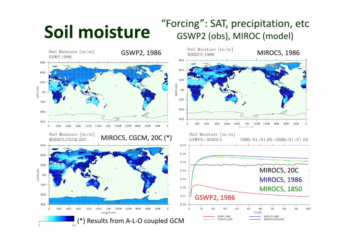
Soil moisture “Forcing”: SAT, precipitation, etcGSWP2 (obs), MIROC (model)
GSWP2, 1986 MIROC5, 1986
GSWP2 (obs), MIROC (model)
MIROC5, CGCM, 20C (*)
MIROC5, 20CMIROC5, 1986MIROC5, 1850
GSWP2, 1986
(*) Results from A‐L‐O coupled GCM

Future challenge: “Nitrogen nexus”Human Society
Climate SystemSociety
Socio‐economicscenario N2O
System
Impacts
Land‐use
scenario
Ecosystem CropModel Fertilizer Residue
yModel
pModel
NO3–
crop production vs pollution?
WaterModelCrop yield
Land‐river‐ocean connectionPotential yield

Future scenarios on nitrogen fertilizergCalculation for potential yield 10 crops: Maize, Rice, Soybean,
Springbarley Springwheatand its quantity of nitrogen fertilizer
Springbarley, Springwheat, Winterbarley, Winterrye, Winterwheat, Sugarbeet, S
Trend estimation for the
Sugercane
4RCP × 5 climate modelsTrend estimation for the
variety of nitrogen fertilizers in the pastin the past
production function
Nitrogen fertilizer scenarios
function
Cropland(Ramankutty et al. 2008)Nitrogen fertilizer scenarios

Future scenarios on nitrogen fertilizerg10 crops: Maize, Rice, Soybean, Springbarley Springwheat
Calculation of potential yield Springbarley, Springwheat, Winterbarley, Winterrye, Winterwheat, Sugarbeet, S
under nitrogen fertilizer input
Sugercane
Estimation of the variety of4RCP × 5 climate models
Crop yield x priceEstimation of the variety of
nitrogen fertilizers in each grid point
Fertilizer input x price
in each grid pointproduction function x price
Maximum incomeNitrogen fertilizer scenarios
function
Cropland(Ramankutty et al. 2008)Fertilizer inputNitrogen fertilizer scenarios

Summary and next stepy p• Land
– Land use modelling downscaling + urban growthLand use modelling, downscaling + urban growth
• Water– Future scenario, water scarcity ‐> Evaluation of future adaptation strategy (water saving etc)
• Ecosystem– Good model for the past uncertain for the future– Good model for the past, uncertain for the future– Management options (geo‐engineering, REDD+ etc)?– Future crop yield (fertilize input, climate change)?
• “Nexus approach” by integration of modelspp y g– Analysis of risk trade‐offs (low‐carbon vs high‐carbon)

A diAppendixModel DescriptionModel Description

Outline of land‐use model Productive ffi i iefficiency in
non-agricultural sectorGeographical
Prices of products
constraint(Slope)
GDPPopulation p
Wedges
l l b l
( p )Population
Populations
Exchange rate
General equilibrium model(Ricardian model base) Exchange rate
Agricultural areaarea
Fertilizer useSpatial
Distribution of Water useCrop yield

Global water resources model H082. Methods
Global water resources model H08
1. High spatial resolution (0.5deg)2. High temporal resolution (daily)3. Interaction between natural water cycle
and human activities
0.50.567,420 cells Human Nature
35Details in http://h08.nies.go.jp/h08/index.html

Ecosystem modelVegetation Integrative Simulator for Trace gases
GHG exchangeVegetation
N‐cycleC‐cycle
Soil
• C budget:stock and flows• GHG exchange:CO2, CH4, N2O• Simple bio‐physical & hydrological scheme• Disturbance:fire, land‐use change etc.• Management options• Vegetation dynamics (under development)

Data assimilation of yield data setinto process based crop model
Global yield data base Technical coefficient Crop growth model
into process‐based crop model
PRYSBI2
Trend of technical coefficientTemperature sensitivity PRYSBI2p yTotal heat unitLeaf structure
MCMC for each grid
RothCIizumi et al. (2013) Glob Ecol & Biogeogr
Global yield data set was assimilated into process‐based model using a Bayesian method p ocess based ode us g a ayes a et odfor maize, soybean, rice, and wheat.