Turk J Elec Eng & Comp Sci

(2016) 24: 1163 – 1175

c⃝ TUBITAK

doi:10.3906/elk-1309-242

Turkish Journal of Electrical Engineering & Computer Sciences

http :// journa l s . tub i tak .gov . t r/e lektr ik/

Research Article

Comparative performance evaluation of blast furnace flame temperature

prediction using artificial intelligence and statistical methods

Yasin TUNCKAYA1,∗, Etem KOKLUKAYA2

1Calık Enerji, Ankara, Turkey2Department of Electrical and Electronics Engineering, Faculty of Engineering, Sakarya University, Sakarya, Turkey

Received: 30.09.2013 • Accepted/Published Online: 18.02.2014 • Final Version: 23.03.2016

Abstract: The blast furnace (BF) is the heart of the integrated iron and steel industry and used to produce melted iron

as raw material for steel. The BF has very complicated process to be modeled as it depends on multivariable process

inputs and disturbances. It is very important to minimize operational costs and reduce material and fuel consumption

in order to optimize overall furnace efficiency and stability, and also to improve the lifetime of the furnace within this

task. Therefore, if the actual flame temperature value is predicted and controlled properly, then the operators can

maintain fuel distribution such as oxygen enrichment, blast moisture, cold blast temperature, cold blast flow, coke to

ore ratio, and pulverized coal injection parameters in advance considering the thermal state changes accordingly. In this

paper, artificial neural network (ANN), multiple linear regression (MLR), and autoregressive integrated moving average

(ARIMA) models are employed to forecast and track furnace flame temperature selecting the most appropriate inputs

that affect this process parameter. All data were collected from Erdemir Blast Furnace No. 2, located in Eregli, Turkey,

during 3 months of operation and the computational results are satisfactory in terms of the selected performance criteria:

regression coefficient and root mean squared error. When the proposed model outputs are considered for the comparison,

it is seen that the ANN models show better performance than the MLR and ARIMA models.

Key words: Blast furnace, prediction, flame temperature, artificial neural networks, multiple linear regression, autore-

gressive integrated moving average

1. Introduction

Blast furnaces (BFs) are a critical part of the manufacturing procedure for the large-scale integrated iron and

steel industry and have working principles totally different from those of electrical arc furnaces, the other

common way of producing steel via melting scrap metal. BFs are built with welded steel plates, platforms,

and piping and are surrounded by refractory bricks on an internal surface basically to resist reactions at higher

temperatures to protect the furnace body and improve internal temperature stability. BFs are relatively large

volume structures and they look like steel chimneys, as shown in Figure 1.

The intention of the present study is to propose novel data classification and mining approaches to analyze

the BF system by dynamic modeling and generate a set of understandable symbolic rules for prediction of flame

temperature, an important control and process parameter to determine the thermal state of the BF. The model

results will act as a guide to help furnace operators in judging temperature change in BFs over time and provide

further indication to determine the direction of controlling the operation in advance.

∗Correspondence: yasin.tunckaya@calikenerji.com

1163

TUNCKAYA and KOKLUKAYA/Turk J Elec Eng & Comp Sci

Figure 1. Physical view of a blast furnace.

Recently, several types of research papers with mathematical modeling and software simulations focusing

on flame temperature prediction and control have been published. The effects of coke charging ratio, performance

of a coke oven gas against blast furnace gas flow under different fuel lance angles, optimization and design of

a burner for oxygen and blast furnace gas injection, linear regression applications considering enthalpy and

heat capacity parameters, and investigations of different gas combinations were studied to model, predict, and

control the flame temperatures in furnaces previously [1–4].

Artificial neural network (ANN), multiple linear regression (MLR), and autoregressive integrated moving

average (ARIMA) models are employed for forecasting in the present paper. The ANN approach is applied

because of its high potential for complex, nonlinear, and time-varying input–output mapping and generally it

is thought to be more powerful than other regression-based techniques [5]. On the other hand, in most of the

studies the results obtained from complex ANN models are compared with those from more standard linear

techniques such as regression and time series analysis for benchmarking [5]. The model results are compared

with each other in terms of the performance criteria regression coefficient (R2) and root mean squared error

(RMSE). The output of the proposed models provided close and satisfactory results for estimation of the flame

temperature in order to provide a best-fit prediction with the observed data.

2. Blast furnace process and flame temperature

The main purpose of chemical reactions during the BF process is to remove oxygen from iron oxides in ore,

creating pig iron as the final product of a BF [6]. This process involves massive combustion and heat transfers

1164

TUNCKAYA and KOKLUKAYA/Turk J Elec Eng & Comp Sci

inside the furnace and an internal temperature over 2000 ◦C. Mainly three raw materials (iron, metallurgical

coke, and limestone) are used in furnaces [7].

Coke is used to raise the furnace’s internal temperature to allow iron ore to be purified. In addition, coke

acts as a reducing agent during that process. Limestone is mainly used as a slag-maker to remove the impurities

of iron ore. Pellet is the main iron ore source in BFs where deposits of ore consist of highly concentrated

iron composition inside as it is found as oxide. In some integrated iron and steel factories, sinter is used as a

secondary iron resource produced in plants using re-cyclic mixing and burning and that material usage plays a

key role in enhancing BF efficiency.

According to the charging principle of BFs, pellet, sinter, coke, and limestone are first arranged in the

material handling and forwarding area of the plant and the materials are charged into the furnace in order using

a high level control of process control systems. Continuously, oxygen is injected inside the pressurized hot blast

composition through tuyere nozzles where a hot blast is supplied using huge air compressors at a power station

and heated up 1100–1200 ◦C by the help of hot stoves. A highly pressurized blast creates a combustion reaction

with coke and internal temperature rises to 2000–2500 ◦C in the furnace.

Meanwhile, carbon monoxide appears due to the combustion of coke and oxygen elements. This gas rises

up through the furnace and removes oxygen from the iron ore. This reaction converts the iron ore to liquid

molten iron and this product falls from the furnace walls to the bottom level as illustrated in Figure 2.

Figure 2. Reactions and temperature regions in a BF.

There are several reactions leading to the furnace process in which pellet, sinter, and limestone materials

are used to reduce oxide and the main chemical reactions are formulated as follows:

3Fe2O3+ −→ CO2 + 2Fe3O4 (1)

Fe3O4 + CO −→ CO2 + 3FeO (2)

FeO + CO −→ CO2 + Fe (3)

FeO + C −→ CO + Fe (4)

1165

TUNCKAYA and KOKLUKAYA/Turk J Elec Eng & Comp Sci

Reactions between impurities in the iron ore and residual limestone create a product, called slag, that floats

on top of the hot metal as it has lower density than pig iron. Therefore, slag is separated from the hot metal

due to that density difference and removed to the slag line to be cooled down. Charged materials reach the pig

iron discharge line in around 5–8 h according to furnace operating conditions. The temperature of hot metal

discharged from the furnace is expected to be between 1400 and 1550 ◦C in normal operation conditions. These

materials are separated as hot metal and slag on the bottom discharge level, commonly a few meters below

tuyere lines. The discharge operation is executed with a tapping procedure, which is performed from furnace

body to furnace heart level [8]. The molten iron is tapped at regular intervals by opening a tap-hole with a

tapping machine.

Hot metal is transferred to the torpedo ladle line to be picked up for chemical enrichment and basic

oxygen furnace process plants. These ladles are surrounded by refractory bricks and capable of storing liquid

hot metal inside without any major heat loss. After chemical material charge into the pig iron to balance

chemical composition in the hot metal according to laboratory results of the samples of pig iron, ladles are sent

through the basic oxygen furnace. The remaining impurities of the molten iron are oxidized by oxygen blasts

injection during this process. This operation results in the production of carbon steel compatible with a range

of international quality standards.

Silicon content in the pig iron and hot metal temperature are major quality indicators for pig iron where

silicon begins entering the furnace through coke ash and iron ore. In high temperature regions, silicon becomes

dissolved in melted iron and relatively high silicon content in pig iron is a sign of ineffective operation of the

furnace. Silicon content in pig iron and hot metal temperature value react in similar ways in the same operation

conditions. This means that if the operators control the hot metal temperature, silicon content is limited to

reasonable values.

The other efficiency criterion, flame temperature, controls the rate of chemical reactions in the combustion

process and has a specific effect in the design of combustion equipment [4]. The main goal is to keep flame

temperature relatively in an operating range to control remaining parameters in any furnace operation. Flame

temperature value is commonly used to control optimum exchange ratios between pulverized coal injection,

steam enrichment, O2 enrichment, and also coke oven gas and blast furnace gas contents in order to heat stoves

up during the process. This parameter has a significant effect on the phase stability as well as final product

characteristics [9].

The actual temperature in a BF body is usually lower than flame temperature as it is calculated neglecting

heat losses in furnaces. Therefore, some of the parameters to calculate flame temperature sometimes do not

reflect realistic values as they rely on assumptions. However, optimum flame temperature is a key reference

point during the continuous process [10]. If the flame temperature begins dropping, then melting capacity and

reduction process will decrease, and thermal heat balance of the furnace will fall. When there is a sudden surge

in flame temperature, the melting zone becomes unstable. If flame temperature rises more than expected values,

the melting zone on tuyere levels will begin increasing.

Pulverized coal injection reduces the flame temperature value. If operators want to prevent flame

temperature drop, hot blast volume or oxygen enrichment value will be increased and blast moisture decreased.

These actions increase the coke burning rate and oxygen concentration in front of the tuyeres. A higher oxygen

concentration causes more chemical reactions and the presence of more CO content. Eventually more CO

increases Fe2O3 reduction in parallel, which means required coke content is reduced and furnace efficiency

increases. The rule based system can help the operators improve the BF’s efficiency by making timely control

adjustments with the goal of minimizing the variation of flame temperature over time.

1166

TUNCKAYA and KOKLUKAYA/Turk J Elec Eng & Comp Sci

3. Proposed models

3.1. Artificial neural networks model

ANNs are inspired by and defined as a functional demonstration of the biological structures of the human

central nervous system. ANNs are commonly used for prediction, matching, identification, pattern recognition,

classification, and optimization of problems [11]. They proved of great use to solve a significant quantity

of complex mathematical problems where complex parameters and lots of variables are involved. They have

multiple advantages: easy to program, present a good adaptation to nonlinear systems, and robust against noise

to adapt to changes in the system conditions [6].

However, modernization of industrial factories using a high level of automation has yielded a huge

volume of data that has to be analyzed and processed [7]. It is reasonable to implement a neural-based

model when there are adequate data on hand to develop new or existing systems accordingly. Prediction

success of ANN models depends on selected input variables [12]. When more input parameters are considered

than required, there will be calculation problems in terms of memory capacity and calculation speed. If fewer

input parameters are considered, model outputs will not be accurate enough to identify the system properly.

Therefore, input parameters should be selected to optimize the system in an appropriate way and reduce the

calculation complexity in parallel [8].

ANNs include a set of simple processing units that communicate by transmitting signals to each other over

a large number of weighted connections. The inputs are multiplied by a weight factor, summed up, computed,

moved, and distributed to the transfer function [13]. The threshold is the magnitude offset that affects the

activation of the node output. Input, hidden, and output layers may have several different variations depending

on model configuration [14]. A neural network structure with input parameters, weights, transfer and activation

functions, and output is shown in Figure 3.

Figure 3. Artificial neural network model.

A neural network model is commonly described with following equation:

oj = φ(

n∑i

xiwnj + b), (5)

where φ represents activation function; xi is input where i = 0, 1, 2,... , n; wnj is weight; b is bias value; and

finally o is output of the neuron. Activation functions can be selected linear or nonlinear type and sigmoid and

1167

TUNCKAYA and KOKLUKAYA/Turk J Elec Eng & Comp Sci

hyperbolic-tangent functions are used in common applications [15]. These functions are used for normalization

and the values are limited between –1 and 1 or 0 and 1. Total error is shown in the following formula at the

output layer:

Total Error =1

2

∑mE2

m (6)

Error = Em = Ym − Exm, (7)

where Exm is expected output value and Ym is obtained output value. The designer should reconsider the

model and change weight factors between interconnections when the total error is bigger than the defined

threshold value. This procedure is used to reduce errors and train the neurons for new calculations, called

the error back propagation process. Back propagation involves two phases: a feed-forward phase in which the

external input information at the input nodes is propagated forward to compute the output information signal

at the output unit, and a backward phase in which modifications to the connection strengths are made based

on the differences between the computed and actual information signals at the output units [5]. The main rule

is to minimize the mean squared differences and error using an iterative procedure between outputs and the

forecasted values [16].

Eventually the weights are updated until the error is limited within acceptable levels. This rule is

called the generalized delta learning rule and is commonly used to supervise the learning algorithm of feed-

forward multilayer neural networks [17]. The most popular learning procedure, called the Levenberg–Marquardt

algorithm, is created by combining the Gauss–Newton and steepest-descent algorithms. The Levenberg–

Marquardt algorithm is capable of minimizing a linear or nonlinear function providing a numerical solution over

a set of parameters, and this optimization algorithm is more powerful than the conventionally used gradient

descent technique [5].

The gradient descent algorithm changes weights and biases proportional to derivatives of the network

in order to minimize the error. The gradient descent algorithm is relatively slow as it requires a smaller

training rate for more stable learning and this is a clear drawback due to its time consuming process. Both the

Levenberg–Marquardt and gradient descent algorithms are used in this study to evaluate possible effects and

performance of the training algorithms of neural networks models. ANNs also can be integrated with many

other approaches including connectionist expert systems to improve the prediction quality further [18].

3.2. Multiple linear regression model

MLR is a statistical model and determines a mathematical relationship between a given set of several inde-

pendent or predictor variables and a dependent variable. MLR is a computationally demanding downscaling

technique and has been widely used in time series analyses and statistics. It is usually less complicated than

its nonlinear counterparts with lower demands regarding computational power, and, unlike nonlinear methods,

without many parameters to be determined prior to application [19]. The model works to create a relationship

between a few or more explanatory variables and a response variable by fitting a linear mathematical equation

to observed data [19]. Each value of the independent variable x is associated with a value of the dependent

variable y [5]. If y is a dependent variable and x1, x2, ..., xi are independent variables, then the basic model

will be given in Eq. (8) below.

y = a+ b1 + x1 + b2x2 + · · ·+ bixi + e, (8)

1168

TUNCKAYA and KOKLUKAYA/Turk J Elec Eng & Comp Sci

where a andbi are constants and e error random variable. The MLR models are an extension of a simple

linear regression model to incorporate two or more explanatory variable in a prediction equation for a response

variable. The constants a, b1, b2, ..., bi are the regression parameters computed by the method of least squares

[5]. Multiple regression modeling is very popular method of statistical analysis in most fields because of its

power and flexibility.

The model requires relatively little effort to compute and estimate complicated models with huge numbers

of variables considering a group of random variables that is trying to find a mathematical relationship between

them. Regression models attempt to make the developed relationship as predictive of the data as possible by

selecting the best weights with which to combine variables, in order to minimize the variance or the mean square

error between the predicted value and the actual value for each observation in the series [20]. That means the

model will forecast exact actual values with some error. More precisely, the goal of regression is to minimize

the sum of the squares of the vertical distances of the points from the line [20].

3.3. Autoregressive integrated moving average model

ARIMA methodology was first developed by Box and Jenkins for forecasting of time series events in 1976 [21].

This model is stated as ARIMA(p, d, q) with the integers where prefers to the autoregressive (AR), d refers

to integrated (I), and q refers to moving average (MA) sections of the data structure. ARIMA models are

used to analyze the historical data in order to provide estimates for the future, and the idea is to separate a

nonstationary series one or more times until the time series becomes stationary, and then find the fit model [22].

Depending on the nature of this process, past observations contain information about future development

and the task is to identify a statistical model that explains the current value of the process as a weighted sum of

past values as autoregressive part, AR, and past error terms as moving average part, MA, where the stochastic

process is assumed to be stationary taking the first difference as integration part, I [23]. The model consists of

four steps of algorithms: identification, estimation, diagnostic checking, and forecasting.

ARIMA is a popular prediction method where each variable is described by its past values and stochastic

error terms. However, when it is applied to nonstationary and huge nonlinear process data, sometimes fore-

casting errors may increase when the forecasting horizon is longer. The pure ARIMA model is described by the

below equation:

Zt = φ1Zt−1 + φ2Zt−2 + . . .+ φpZt−p + at + θ1at−1 + θ2at−2 + . . .+ θqat−q, (9)

where p , d , and q describe the integer parameters of the ARIMA model; φp describes the parameters for

autoregressive operator; at describes the parameters of error term; θq describes the parameters of moving

average operator; and Zt describes the time series of d order difference term of original series.

4. Materials and methods

The BF process consists of hundreds of variables stored, monitored, or controlled using high level automation

systems while some of the variables directly affect flame temperature, some of them with minimum or no

influence.

The parameters shown in Table 1 are selected for this paper as the most effective in order to predict

flame temperature due to previous experience and recommendation by furnace operation engineers. The

input parameters are described with engineering units, and minimum, maximum, and average operation values

according to the sample data set.

1169

TUNCKAYA and KOKLUKAYA/Turk J Elec Eng & Comp Sci

Table 1. Selected input parameters.

Selected input parameters Min. value Max. value Average value Eng. unitsCold blast flow 2561.90 3612.25 3379.18 Nm3/minCold blast temperature 984.05 1113.62 1071.59 ◦CAdditional O2 flow 106.90 178.05 163.86 Nm3/minAdditional steam injection 18.61 28.33 21.93 g/Nm3

Pulverized coal injection rate 13.84 35.45 27.63 T/hBlast pressure 1.94 3.17 2.93 Bar

Graphical trends of the cold blast temperature, oxygen enrichment, additional steam injection, cold blast

temperature, blast pressure, and pulverized coal injection rate are shown in Figure 4 during 24 h of operation as

a reference since it can be seen that the rates are changing very fast due to instantaneous operating conditions

and operator interventions. Various kinds of abnormalities sometimes occur during furnace operation and the

estimation of the cause of the abnormalities and the performance of necessary actions are compulsory for the

long-term control of furnace operation [24].

31003150320032503300335034003450

42210

Cold Blast Flow-Nm /min

145

150

155

160

165

170

42210

O2 Injection -Nm /min

25

30Steam Injection -g/Nm

11001120

Cold Blast Temperature -°C3

3 3

0

5

10

15

20

42210980

10001020104010601080

42210

5

10

15

20

25

30Pulverized Coal Injection Rate -T/h

2.7

2.8

2.9

3

3.1

3.2Blast Pressure-Bar

042210

2.642210

Figure 4. Values of the variables used in the model during a period of 24 h.

The process control system records the data when the new measurement is carried out, and repeats

this value until the next measurement [25]. In order to define sampling rates of the variables before usage

in the model, interpolation is used to obtain regularly distributed values in the same period of time. Several

models can be used for nonlinear systems such as NFIR, NARX, NOE, NARMAX, and NBJ. NARX (Nonlinear

AutoRegresive models with eXogenous input) is chosen for the ANN model structure that is described with the

1170

TUNCKAYA and KOKLUKAYA/Turk J Elec Eng & Comp Sci

below equation:

yˆ(k) = F (y(k − 1), y(k − 2), ..., y(k − p), ..., u(k), u(k − 1), ..., u(k − q)) (10)

The forecasted value of variable y for sampling time k is considered as a function of the values taken by this

variable at the p previous sampling times and of the values of the input variables, generically represented by u

at the previous sampling times q [25].

After definition of the NARX model for the ANN approach, the next step will be the selection of a neural

network as a feed forward model is considered for the study. Some of the variables executed directly in the

model and remaining parameters were preprocessed before the execution to reduce the total quantity of past

data and prevent use of new model inputs.

Hidden layer neuron quantity is a critical parameter that depends on the researcher’s experimental

decision. The design should be identified according to the complexity of the problem in order to achieve

successful results. Before training and testing, all the data are scaled using the extremes between 0 and 1 for

each neural network model as given in Eq. (11).

xscaledi =

xi − xmin

xmax − xmin, (11)

where xi , xmax , and xmin are the original, the maximum, and the minimum values, respectively. MATLAB

R2009b was used for the training of neural networks since it is possible to change transfer functions, training

algorithm, % of trained neurons, etc. using this toolbox. Total data were divided into the three following

groups: training, verification, and testing.

In total 1728 collected data items for 6 input and 1 output parameters during 5 s of operating time

were used in the ANN model during 3 working months of the Erdemir No. 2 BF. While 60% of the data were

used for training, 15% were used for validation and the remaining 25% for testing purposes. The Levenberg–

Marquardt algorithm was employed to train the neurons. The method of trial and error was employed to select

suitable quantities of hidden neurons and hidden layers. Four neurons in one hidden layer were considered after

experimental studies.

Model outputs and the comparison of actual and predicted flame temperature for 432 tested values are

shown in Figure 5 below. Blue color shows the predicted values and red color refers to actual values of flame

temperature. It is seen that both actual and forecasted values almost overlap and track each other, which meant

that the proposed model works quite successfully.

2100

2150

2200

2250

2300

2350Predicted & Actual Flame Temperatures

Predicted Flame Temperature (Deg C)

Actual Flame Temperature (Deg C)

Figure 5. ANN model results for actual and predicted flame temperatures.

According to ANN prediction results, it is apparent that the model can recognize positive and negative

movements of the temperature values on time and successfully. The maximum prediction error is 23.14 ◦C

1171

TUNCKAYA and KOKLUKAYA/Turk J Elec Eng & Comp Sci

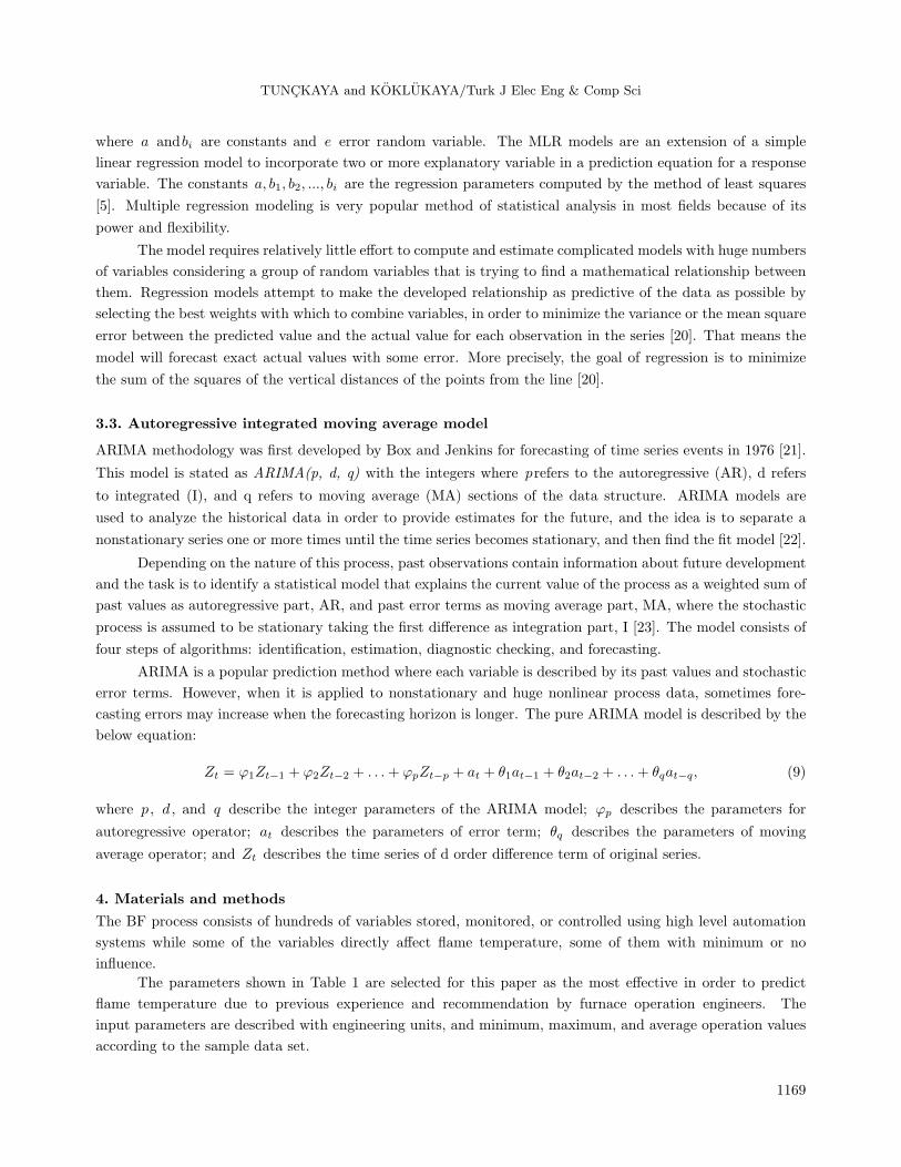
and it is seen that the average errors are distributed between 0 and 10 ◦C. Figure 6 shows the error rates

between the actual and predicted temperatures of the first ANN model with the Levenberg–Marquardt training

algorithm.

–30

–20

–10

0

10

20

30 Error Between Actual and Predicted Flame Temperatures

ERROR (Deg C)

Figure 6. ANN model error rates between actual and predicted flame temperatures.

There are very limited peak errors above 20 ◦C, which means 0.008% difference from the actual tem-

perature value, as unstable operations and extreme interventions may sometimes affect the overall operation.

Average absolute error between the actual and predicted set of values is 4.45 ◦C. Moreover, 99.93% of pre-

dicted flame temperature values do not differ more than 10 ◦C from the actual temperature values and this

performance shows the accuracy of the model better.

In the second phase of this study, the training algorithm of the neural network is changed to gradient

descent instead of Levenberg–Marquart to evaluate the effects of the training algorithm selection on error rates

and overall performance. The same input, hidden, and output layers and flame temperature data were used and

all settings were kept in order to have an exact comparison. The outputs of the second ANN model show that

the gradient descent algorithm is time consuming and shows worse performance than the other ANN model.

Finally the proposed statistical models, MLR and ARIMA, were executed using the same parameters and

data. The independent variables of the MLR and ARIMA models are the input nodes of the ANN model and the

calibration period is selected along with the ANN training duration. Again, in total 1728 data items collected

during 5 s of operating time were considered as 6 independent parameters against the dependent parameter,

the flame temperature. IBM SPSS Version 17.0 was used for the MLR and ARIMA modeling as this software

has intensive and flexible parameter settings and used as a reference statistical tool in the present studies. All

p, d, and q parameters are selected 1 for each ARIMA(1, 1, 1) model.

The ANN, MLR, and ARIMA models are compared using the following performance criteria: regression

coefficient and root mean squared error. Regression coefficient describes a degree of collinearity between

simulated and measured data; the regression coefficient, ranging from –1 to 1, is an index of the degree of

linear relationship between actual and simulated data [26]. When the regression coefficient is 0, no linear

relationship exists. However, if it is 1 or –1, a perfect positive or negative linear relationship between these two

types of data exists. Similarly, coefficient of determination describes the proportion of the variance in measured

data explained by the model and R2 ranges from 0 to 1, with higher values indicating less error variance, and

typically values greater than 0.5 are considered acceptable [26]. R2 value is used as a comparison factor and

correlation criterion in the present paper.

RMSE is a widely used parameter of the differences between values forecasted by a model or an estimator

and the observed values actually. It is a measure of reliability and efficiency for actual and predicted data sets

1172

TUNCKAYA and KOKLUKAYA/Turk J Elec Eng & Comp Sci

and defined below [26]:

RMSE =

√1

n

∑n

i=1

(Y obsi − Y sim

i

)2, (12)

where Y obsi is observed value, Y sim

i is predicted value, and n is number of samples. When the RMSE value is

reduced, it means that the error is minimized and the system gives a more efficient performance. The comparison

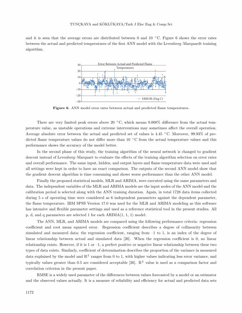
between the proposed models after several simulations is shown in Table 2 as a summary of this research.

Table 2. Comparison of the model outputs.

Comparison parametersANN ANN ARIMA MLRmodel - 1 model - 2 model model

RMSE 7.203 7.405 8.274 8.789R2 0.964 0.945 0.907 0.892Min. flame temp. (◦C) 2171.501 2169.035 2164.284 2156.103Max. flame temp. (◦C) 2345.394 2340.578 2347.968 2343.809Mean flame temp. (◦C) 2303,556 2240.893 2243.271 2240.364

According to MLR and model outputs, the regression between dependent variable flame temperature and

remaining independent variables is 0.892 and 0.907, respectively, which shows that there is a strong correlation

with selected parameters affecting the flame temperature values. When the ANN approach using the Levenberg–

Marquardt and gradient descent training algorithms are considered, the regression coefficients are 0.964 and

0.945, respectively, as per model outputs. Consequently, the neural network models show better performance

than the MLR and ARIMA models in terms of correlation criteria. MLR model outputs show that the minimum

flame temperature is 2156.103 ◦C, maximum flame temperature is 2343.809 ◦C, and mean is 2240.364 ◦C, while

ARIMA model outputs show a minimum flame temperature of 2164.284 ◦C, maximum flame temperature of

2347.968 ◦C, and mean of 2243.271 ◦C.

RMSE is calculated as 7.203 and 7.405 for the Levenberg–Marquardt and gradient descent algorithms

in the ANN models, and 8.789 and 8.274 for MLR and ARIMA models, respectively. As the ANN model has

a lower RMSE value than MLR and ARIMA, it is seen that both ANN models have better performance than

the MLR and ARIMA models in terms of RMSE and R2 criteria. It is also concluded that the ARIMA modelshows a slightly better performance than MLR.

5. Conclusions

In this paper, the flame temperature of the Blast Furnace No. 2 in Eregli, Turkey, is modeled using ANN, MLR,

and ARIMA models considering 6 process parameters that directly affect that temperature. These models are

set up, computed, and executed using Mathworks MATLAB and IBM SPSS, as these tools are easy to configure

and change model settings during execution of the calculations. The flame temperature movement is crucial

information to instruct the furnace operation team for necessary interventions and corrective actions playing

with furnace parameters immediately in order to control the overall furnace operation. The proposed prediction

system proves its accuracy and reliability to track the temperature movements and fluctuations properly as per

the experimental studies.

Model results verified that the error rate and temperature drift between predicted and actual flame

temperatures are quite limited and the model tracks temperature regime very well. Compared with the

previous research on BF process parameter predictions [17,25], it is shown that the prediction success for

1173

TUNCKAYA and KOKLUKAYA/Turk J Elec Eng & Comp Sci

flame temperature has been improved up to 99.93% against maximum 10 ◦C error with the first ANN model

where the Levenberg–Marquardt training algorithm is used and the error rate is minimized relatively within

this paper.

Based on this study, the following specific conclusions can be summarized as follows:

• Artificial neural network models have better performance than multiple linear regression and autoregressive

integrated moving average models as per the performance criteria: R2 and RMSE,

• The Levenberg–Marquardt training algorithm has shown better performance than the gradient descent

algorithm in terms of ANN forecasting success,

• Flame temperature can be tracked using the ANN scheme accurately where the proposed model can

predict smooth and extreme temperature movements perfectly,

• Selected prediction parameters have very high regression with the flame temperature parameter and it is

shown that these parameters affect the temperature changes directly,

• Tracking of the flame temperature value increases operator awareness, and also furnace efficiency and

stability in parallel,

Further to this study, a Level 2 suggestion system can be developed to lead operators for further actions

using the proposed model and set points of the mentioned parameters can be automatically adjusted via DCS

control system integration in future.

References

[1] Mroz J. Current Situation and Predictions further development of Blast Furnace Technology. Journal of Achieve-

ments in Materials and Manufacturing Engineering 2012; 55: 889-894.

[2] Hellberg P, Jonsson TLI, Jonsson PG, Sheng DY. A Model of Gas Injection into a Blast Furnace Tuyere. Fourth

International Conference on CFD in the Oil and Gas Metallurgical & Process Industries: SINTEF/NTNU Norway

2005; 1; 1.

[3] Hooney PL, Boden A, Wang C, Grip C, Jansson B. Design and application of a spreadsheet based model of the

blast furnace factory. ISIJ International 2010; 50: 924-930.

[4] Asl ZM, Salem A. Investigation of the flame temperature for some gaseous fuels using artificial neural network.

International Journal of Energy and Environmental Engineering 2010; 1: 57-63.

[5] Ustaoglu B, Cigizoglu HK, Karaca M. Forecast of daily mean, maximum and minimum temperature time series by

three artificial neural network methods. Meteorological Applications 2008; 15: 431-445.

[6] Kirk O. Encyclopedia of Chemical Technology. 13th ed. New York, NY, USA: John Wiley and Sons, 1981.

[7] Garcia FA, Campoy P, Mochon J, Ruiz-Bustinza I, Verdeja LF, Duarte RM. A new “user-friendly” blast furnace

advisory control system using a neural network temperature profile classifier. ISIJ International 2010; 50: 730-737.

[8] Danforth GW. An Elementary Outline of Mechanical Processes. 2nd ed. USA: The United States Naval Institute,

1917.

[9] Ghosh SK, Pal S, Roy SK, Pal SK, Basu D. Modelling of flame temperature of solution combustion synthesis of

nanocrystalline calcium hydroxyapatite material and its parametric optimization. Bull Mater Sci 2010; 33: 339-350.

[10] Bidabadi M, Rahbari A. Novel analytical model for predicting the combustion characteristics of premixed flame

propagation in lycopodium dust particles. J Mech Sci Technol 2009; 23: 2417-2423.

1174

TUNCKAYA and KOKLUKAYA/Turk J Elec Eng & Comp Sci

[11] Radhakrishnan VR, Mohamed AR. Neural Networks for the Identification and Control of Blast Furnace Hot Metal

Quality. J Process Contr 2010; 10: 509-524.

[12] Wang Y, Liu X. Prediction of Silicon Content in Hot Metal Based on SVM and Mutual Information for Feature

Selection. Journal of Information & Computational Science 2011; 8: 4275-4283.

[13] Arzuman S. Comparison of Geostatistics and Artificial Neural Networks in Reservoir Property Estimation. PhD

Thesis, Middle East Technical University, Ankara, Turkey, 2009.

[14] Daliri MR, Fatan M. Improving the Generalization of Neural Networks by Changing the Structure of Artificial

Neuron. Malayas J Comput Sci 2011; 24: 195-204.

[15] Yaakob SN, Saad P. Generalization performance analysis between Fuzzy Artmap and Gaussian Artmap neural

network. Malayas J Comput Sci 2007; 20: 13-22.

[16] Dalgakıran I, Danısman K. Artificial neural network based chaotic generator for cryptology. Turk J Elec Eng &

Comp Sci 2010; 18: 225-240.

[17] Perez-Cruz JH, Alanis AY, Rubio JJ, Pacheco J. System identification using multilayer differential neural networks:

a new result. J Appl Math 2012; Article ID 529176; 20.

[18] Shi SM, Xu LD, Liu B. Improving the accuracy of nonlinear combined forecasting using neural networks. Expert

Syst Appl 1999; 16: 49-54.

[19] Holder RL. Multiple Regression in Hydrology. 1st ed. Wallingford, UK: Institute of Hydrology Press, 1985.

[20] Alhadidi B, Al-Afeef A, Al-Hiary H. Symbolic regression of crop pest forecasting using genetic programming. Turk

J Elec Eng & Comp Sci 2012; 20: 1332-1342.

[21] Box GEP, Jenkins G. Time Series Analysis. Forecasting and Control. San Francisco, CA, USA: Holden-Day, 1976.

[22] Al-Wadi S, Ismail MT. Selecting wavelet transforms model in forecasting financial time series data based on ARIMA

model. Applied Mathematical Sciences 2011; 5: 315-326.

[23] Huwiler M, Kaufmann D. Combining Disaggregate Forecasts for Inflation: The SNB’s ARIMA model, 7th edition:

Swiss National Bank Economic Studies, 2013.

[24] Otsuka K, Matoba Y, Kajiwara Y, Kojima M, Yoshida M. A hybrid expert system combined with a mathematical

model for blast furnace operation. ISIJ International 1990; 30: 118-127.

[25] Jimenez J, Mochon J, Ayala JS, Obeso F. Blast furnace hot metal temperature prediction through neural networks-

based models. ISIJ International 2004; 44: 573-580.

[26] Moriasi DN, Arnold JG, Van Liew MW, Bingner RL, Harmel RD, Veith TL. Model evaluation guidelines for

systematic quantification of accuracy in watershed simulations. T ASABE 2007; 50: 885-900.

1175