Comparing Classical Test Theory with CFA and How … · Comparing Classical Test Theory with CFA ‐and‐ How To Use Test Scores in Secondary Analyses Latent Trait Measurement and

Comparing Classical Test Theory with CFA‐and‐

How To Use Test Scores in Secondary Analyses

Latent Trait Measurement and Structural Equation Models

Lecture #8March 6, 2013

PSYC 948: Lecture #8

Today’s Class

• Comparing classical test theory to CFA The use and misuse of sum scores Reliability for sum scores under CFA

• How to use CFA to test assumptions in CTT

• What to do when SEM isn’t an option Secondary analyses

PSYC 948: Lecture #8 2

Data for Today’s Class

• Data were collected from two sources: 144 “experienced” gamblers

Many from an actual casino 1192 college students from a “rectangular” midwestern state

Many never gambled before

• Today, we will combine both samples and treat them as homogenous – one sample of 1346 subjects Later we will test this assumption – measurement invariance (called differential item functioning in item response theory literature)

• We will build a scale of gambling tendencies using the first 24 items of the GRI Focused on long‐term gambling tendencies


Pathological Gambling: DSM Definition

• To be diagnosed as a pathological gambler, an individual must meet 5 of 10 defined criteria:


1. Is preoccupied with gambling 2. Needs to gamble with increasing

amounts of money in order to achieve the desired excitement

3. Has repeated unsuccessful efforts to control, cut back, or stop gambling

4. Is restless or irritable when attempting to cut down or stop gambling

5. Gambles as a way of escaping from problems or relieving a dysphoricmood

6. After losing money gambling, often returns another day to get even

7. Lies to family members, therapist, or others to conceal the extent of involvement with gambling

8. Has committed illegal acts such as forgery, fraud, theft, or embezzlement to finance gambling

9. Has jeopardized or lost a significant relationship, job, educational, or career opportunity because of gambling

10. Relies on others to provide money to relieve a desperate financial situation caused by gambling

4

Final 12 Items on the Scale

Item Criterion Question

GRI1 3 I would like to cut back on my gambling.

GRI3 6If I lost a lot of money gambling one day, I would be more likely to want to play again the following day.

GRI5 2I find it necessary to gamble with larger amounts of money (than when I first gambled) for gambling to be exciting.

GRI6 8 I have gone to great lengths to obtain money for gambling.

GRI9 4 I feel restless when I try to cut down or stop gambling.

GRI10 1 It bothers me when I have no money to gamble.

GRI11 5 I gamble to take my mind off my worries.GRI13 3 I find it difficult to stop gambling.

GRI14 2 I am drawn more by the thrill of gambling than by the money I could win.

GRI15 7 I am private about my gambling experiences.GRI21 1 It is hard to get my mind off gambling.

GRI23 5 I gamble to improve my mood.


• The 12 item analysis gave this model fit information:

GRI 12 Item Analysis


The model indicated the model did not fit better than the saturated model – but this statistic can be overly sensitive

The model RMSEA indicated good model fit (want this to be < .05)

The model CFI and TLI indicated the model fit well (want these to be > .95)

The SRMR indicated the fit well (want this to be < .08)

CLASSICAL TEST THEORY


Classical Test Theory (CTT)

• What you have learned about measurement so far likely falls under the category of CTT: Writing items and building scales Item analysis Score interpretation Evaluating reliability and construct validity

• Big picture: We will view CTT as model with a restrictive set of assumptions within a more general family of latent trait measurement models Confirmatory Factor Analysis is a measurement model


Differences Among Measurement Models

• What is the name of the latent traitmeasured by a test? Classical Test Theory (CTT) = “True Score” (T) Confirmatory Factor Analysis (CFA) = “Factor Score” (F) Item Response Theory (IRT) = “Theta” (θ)

• Fundamental difference in approach: CTT unit of analysis is the WHOLE TEST (item sum or mean)

Sum = latent trait, and the sum doesn’t care how it was created Only using the sum requires restrictive assumptions about the items

CFA, IRT, and beyond unit of analysis is the ITEM Model of how item response relates to an estimated latent trait Different models for differing item response formats Provides a framework for testing adequacy of measurement models


Classical Test Theory (CTT)

• In CTT, the TEST is the unit of analysis: True score T:

Best estimate of ‘latent trait’: Mean over infinite replications Error e:

Expected value (mean) of 0, expected to be uncorrelated with T e’s are supposed to wash out over repeated observations

So the expected value of T is Ytotal In terms of observed variance of the test scores:

Observed variance = true variance + error variance

• Goal is to quantify reliability Reliability = true variance / (true variance + error variance)

• Because the CTT model does not include individual items, items must be assumed exchangeable (and more items is better)


Ytotal

TrueScore

error

?

?

10

Classical Test Theory, continued

• CTT unit of analysis is the WHOLE TEST (sum of items) Want to ascertain how much of observed test score variance is due to ‘true score’ variance versus ‘error’ variance

Quantify ‘error variance’ in various ways ‘Error’ is a unitary construct in CTT (and error is ‘bad’) Goal is then to reduce ‘error’ variance as much as possible

Standardization of testing conditions (make confounds constants) Aggregation = more items are better (errors should cancel out)

Items are exchangeable; properties are not taken into account

• Followed by generalizability theory to decompose error e.g., rater variance, person variance, time variance


Advantages of CFA over CTT

• More reasonable assumptions about items CTT assumes tau‐equivalent items

Tau – equivalent items: equal factor loadings CFA allows a test of whether each item relates to the factor, as well as whether different factor loadings across items are needed Would indicate some items are better than others

• Comparability across samples, groups, and time CTT: No separation of observed item responses from true score

Sum across items = true score; item properties are for that sample only CFA: Latent trait is estimated separately from item responses

Separates person traits from specific items given Separates item properties from specific persons in sample

• Advantages apply to any latent trait model


Reliability Measured by Alpha

• For quantitative items (items with a scale – although used on categorical items), this is Cronbach’s Alpha… Or ‘Guttman‐Cronbach alpha’ (Guttman 1945 > Cronbach 1951) Another reduced form of alpha for binary items: KR 20

• Alpha is described in multiple ways: Is the mean of all possible split‐half correlations Is expected correlation with hypothetical alternative form of the same length

Is lower‐bound estimate of reliability under assumption that all items are tau‐equivalent (more about that later)

As an index of “internal consistency” Although nothing about the index indicates consistency!


Where Alpha Comes From

• The sum of the item variances is given by: Var(I1) + Var(I2) + Var(I3)…. + Var(Ik) (just the item variances)

• The variance of the sum of the items is given by the sum of ALL the item variances and covariances: Var(I1 + I2 + I3) = Var(I1) + Var(I2) + Var(I3) …

+ 2Cov(I1,I2) + 2Cov(I1,I3) + 2Cov(I2,I3) … Where does the ‘2’ come from?

Covariance matrix is symmetric Sum the whole thing to get to thevariance of the sum of the items


I1 I2 I3I1 σ12 σ12 σ13

I2 σ21 σ22 σ23

I3 σ31 σ32 σ32

14

Guttman‐Cronbach Alpha for Reliability

• Numerator reduces to just the covariance among items Sum of the item variances…

Var(X) + Var(Y) = Var(X) + Var(Y) just the item variances Variance of total Y (the sum of the items)…

Var(X+Y) = Var(X) + Var(Y) + 2Cov(X,Y) PLUS covariances So, if the items are related to each other, the variance of the total Y item sum should be bigger than the sum of the item variances How much bigger depends on how much covariance among the items – the primary index of relationship


Covariance Version:k = # items

15

Assessing Reliability in Our 12 Item Gambling Scale

• To get the Guttman‐Chronbach Alpha of our 12 item scale, we need the covariance matrix This can be found by the SAMPSTAT option under the OUTPUT statement

Sum of item variances = 11.834 Sum of item covariances = 21.575 Variance of Total Y = 11.834+2*21.575 = 54.984

• Alpha reliability: . ..

.852


Reliability…for what?

• The alpha reliability is the reliability for: The total test score Under the assumption that the items are tau‐equivalent

Tau‐equivalent means each item contributes equally In a few slides, we will see how this translates to CFA

• What alpha is not: An index of model fit (unidimensionality)


Measurement Language: Don’t Say These

• Often, people refer to items as “tapping” some latent trait I think this makes the process less transparent – items measure the trait

• When alpha is used, you can sometimes hear people say something about how well the items “hang together” This is certainly not true…


How to Get Alpha UP


Alpha as Reliability… What could go wrong?

• Alpha does not index dimensionality it does not index the extent to which items measure the same construct

• The variability across the inter‐item correlations matters, too!• We use item‐based models (CFA) to examine dimensionality


Case In Point: All 24 Items

• Last class we showed that the 24 items of the GRI did not fit a one‐factor model – what would happen if we neglected to check model fit and used the total score as our estimate of gambling tendency?

• The reliability estimate – from the covariance matrix of all the items (the saturated model H1) was .861 We would have concluded we had a “good” scale for gambling

• But, from CFA last week, we found that one factor didn’t describe all the items Any subsequent analysis will have the misfit bias the results


Testing CTT Assumptions in CFA

• Alpha is reliability assuming two things: All factor loadings (discriminations) are equal, or that the items are “true‐score equivalent” or “tau‐equivalent”

Local independence (dimensionality now tested within factor models)

• We can test the assumption of tau‐equivalence too via nested model comparisons in which the loadings are constrained to be equal –does model fit get worse? If so, don’t use alpha – use model‐based reliability (omega) instead. Omega assumes unidimensionality, but not tau‐equivalence

Research has shown alpha can be an over‐estimate or an under‐estimate depending on particular data characteristics

• The assumption of ‘Parallel items’ is then testable by constraining item error variances to be equal, too – does model fit get worse? ‘Parallel items’ will hardly ever hold in real data Note that if tau‐equivalence doesn’t hold, then neither does ‘parallel’


Another Blast from the Past: Parallel Items

• Another CTT “model” that exists that of parallel items All items have the same covariance and variance Goes one step further than tau equivalence (equal covariances but unequal variances)

• Under the parallel items model, the alpha reliability for the total test score is called the Spearman‐Brown reliability Used to “prophesy” the number of items needed to increase reliability to a desired level

• Spearman‐Brown Prophesy FormulaReliabilityNEW = ratio*relold / [(ratio‐1)*relold + 1]

Ratio = ratio of new #items to old #itemsFor example:

Old reliability = .40Ratio = 5 times as many items (had 10, what if we had 50)New reliability = .77


Reliability vs. Validity “Paradox”

• Given the assumptions of CTT, it can be shown that the correlation between a test and an outside criterion cannot exceed the reliability of the test (see Lord & Novick 1968) Reliability of .81? No observed correlations possible > .9, because that’s all the ‘true’ variance there to be relatable!

In practice, this may be false because it assumes that the errors are uncorrelated with the criterion (and they could be)

• Selecting items with the strongest discriminations (or the strongest inter‐correlations) can help to ‘purify’ or homogenize a test, but potentially at the expense of construct validity Can end up with a ‘bloated specific’ Items that are least inter‐related may be most useful in keeping the construct well‐defined and thus relatable to other things


Using CTT Reliability Coefficients: Back to the Score Estimates

• Reliability coefficients are useful for describing the behavior of the test in the overall sample… Var(Y) = Var(T) + Var(e)

• But reliability is a means to an end in interpreting a score for a given individual –we use it to get the error variance

Var(T) = Var(Y)*reliability; so Var(e) = Var(Y) – Var(T) 95% CI for individual score = Y ± 1.96*SD(e) Gives an indication of how precise the true score estimate is on the metric of the original variable

Example: Y = 100, Var(e) = 9 95% CI ≈ 94 to 106Y = 100, Var(e) = 25 95% CI ≈ 90 to 110

Note this assumes a symmetric distribution, and thus will go out of bounds of the scale for extreme scores

Note this assumes the SD(e) or the SE for each person is the same Cue mind‐blowing GRE example


95% Confidence Intervals: QuantitativeSEM ranges from 9 to 55


REVISITING CTT FROM A CFA PERSPECTIVE


Classical Test Theory from a CFA Perspective

• In CTT the unit of analysis is the test score:,

• In CFA the unit of analysis is the item:

• To map CFA onto CTT, we must put these together:

,


Further Unpacking of the Total Score Forumla

• Because CFA is an item‐based model, we can then substitute each item’s model into the sum:

,

• Mapping this onto true score and error from CTT:

and


Familiar Terms

• The tau‐equivalent model assumes: All items measure the factor the same: Each item has its own unique variance: ∼ 0,

• The parallel items models assumes: All items measure the factor the same: All items have the same unique variance: ∼ 0,

• As such, each of these models can be tested by using the CFA approach – each are nested within the full CFA model


Tau‐Equivalence: Model Implied Covariance Matrix

• The CFA model implies a very specific form for the covariance matrix of the observed items:

• The variance of an item was:• The covariance of a pair of items and was:

• Under Tau‐Equivalence, all loadings are the same, meaning: The item variances can be different (because of ) All item covariances are the same ( )

• This is called the compound symmetry heterogeneous model We can actually achieve the same model without the factor


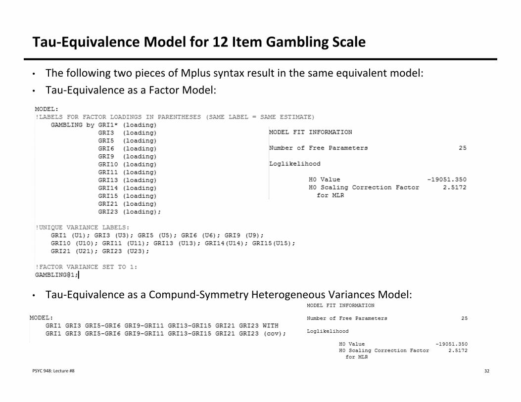
Tau‐Equivalence Model for 12 Item Gambling Scale

• The following two pieces of Mplus syntax result in the same equivalent model:• Tau‐Equivalence as a Factor Model:

• Tau‐Equivalence as a Compund‐Symmetry Heterogeneous Variances Model:


Model Implied Covariance Matrix

• All covariances equal/all variances different


Testing for Tau Equivalence

• The Tau‐Equivalence model (assumed when you sum items) can be tested against the full CFA model The models are nested, so we can use a likelihood ratio test

• Log‐likelihood from CFA model: ‐18,988.425; SCF = 2.4309 36 parameters (12 item intercepts, 11 factor loadings, 1 factor variance, 12 unique variances)

• Log‐likelihood from TE model: ‐19,051.350; SCF = 2.5172 25 parameters (12 item intercepts, 1 factor loading, 12 unique variances)

• MLR Likelihood ratio test: 56.315, .001

• Therefore, we reject the tau‐equivalent model in favor of the CFA model – this means the simple sum of the items is not sufficient We should use the CFA model factor score instead of a sum score


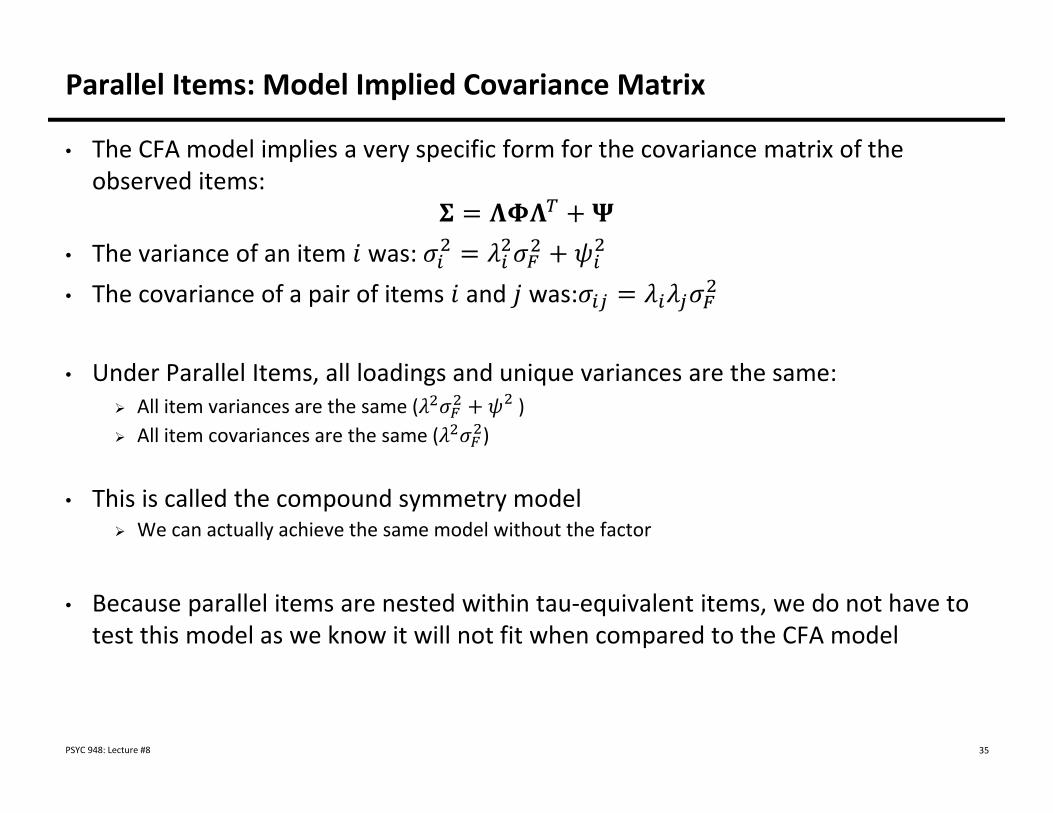
Parallel Items: Model Implied Covariance Matrix

• The CFA model implies a very specific form for the covariance matrix of the observed items:

• The variance of an item was:• The covariance of a pair of items and was:

• Under Parallel Items, all loadings and unique variances are the same: All item variances are the same ( ) All item covariances are the same ( )

• This is called the compound symmetry model We can actually achieve the same model without the factor

• Because parallel items are nested within tau‐equivalent items, we do not have to test this model as we know it will not fit when compared to the CFA model


Test Score Reliability Under the CFA Model

• Coefficient alpha gave reliability for the total test score under the Tau‐Equivalent Items Model We rejected that model in favor of the CFA model Therefore, coefficient alpha will not be correct for our total test score (if we were to still sum up the items)

• The notions of test score reliability under the CFA model now involve the factor loadings But still come back to classical notion of reliability being the proportion of variance due

to true score:


Deriving Reliability For Sum Scores Under the CFA Model

• To show where total‐score reliability under the CFA model comes from, recall our CFA‐model for the total score:

,

• Mapping this onto true score and error from CTT:

and

• We now must derive the variance for T and E


True Score Variance Under the CFA Model

• The variance for the true score:


Error Variance Under the CFA Model

• Because the CFA model allows for the estimation of error covariances (although you shouldn’t do that), the error variance under the CFA model becomes:

• When error covariances are not estimated, the last term is zero, leaving


Reliability for Total Score Under CFA

• The reliability of the total score from CFA, is then:∑

∑ ∑ ∑ ∑ 2 ,• This reliability coefficient is called coefficient Omega ( )

• If the tau‐equivalent model does not hold is the reliability of a total test score (sum score) Typically is higher than Alpha If unidimensional model holds, coefficients will be close


Calculating Omega for Our Test

• We can use Mplus to calculate Omega for our test:


Here, Omega is .855

41

Omega Under Tau‐Equivalent Items

• Omega equal to Alpha when you use the tau‐equivalent items model Omega is the Spearman Brown reliability under parallel items


Here, Omega is .852 –which is equal to the Alpha we calculated using the covariance matrix

42

Recapping: CTT using CFA

• Classical test theory – and more specifically, total test scores, is the dominant way to assess subjects This is true even under CFA

• The key is to be sure to check if a one‐factor model fits the data before using any type of reliability coefficient If not, do not use a test score

• If the one factor model fits – then a single score can represent the test

• The next worry is about representing the error in the test score (related to reliability) If reliability is “high” (? How high, standard of .8), then using the test score in a subsequent analysis is accepted practice


Secondary Analyses with Factor Scores

• If you want to use results from a survey in a new analysis Best: Use SEM – error in factor scores is already partitioned variance

Similarly good: Use “plausible values” (repeated draws from posterior distribution of each person’s factor score) – essentially what SEM does – but with factor scores that vary within a person Can be done in Mplus – not described

Slightly Less Good: Use SEM with “single indicator” factors using sum scores The focus of the next section Make error variance = (1‐reliability)*Variance (Sum score); factor loading = 1

Okay (but widespread): for scales that are unidimensional (and verified in CFA), use sum scores Assumes unidimensionality and “high” reliability

Not Cool: Use factor scores only


What about Using Factor Scores?

• Although CFA factor scores have fewer problems than EFA factor scores (because there is no rotation in CFA), they still have issues: They will be shrunken (i.e., pushed towards the mean, such that the observed variance of the factor scores will be less than the original factor variance)

Can get estimates of “factor determinacy” how correlated estimated factor scores are with true factor scores (basically how much error is introduced by estimating the factor scores as observed variables)

They are just estimates of central tendency from a distribution for each person, not known values – and using estimates as known values in another model makes the relationships within that model look more precise than they are (like SE = 0)

You CANNOT create factor scores by using the loadings as such: F = λ11y1 + λ21y2 + λ21y3… This is a COMPONENT model, not a FACTOR model.


SINGLE INDICATOR MODELS


Single Indicator Models

• Single indicator models are CFA‐like models where a “factor” is measured by a single indicator: Shown here for the gambling factor


Gambling Tendencies

Sum of 10 GRI Items

,

1

1

47

Identification in Single Indicator Models

• How is this possible? Isn’t a single indicator factor model unidentified? We fix the factor variance, factor loading, and unique variance Factor variance represents “reliable” portion

• Single indicator model parameters: ‐ factor variance; ‐ factor loading; ‐ item unique variance (assume factor mean fixed to

zero and item intercept is set to it mean)

• Our constraints are: 1 ∗ (the portion of Y that is “reliable”) 1 ∗ (the portion of Y that is left over)


Assumptions in a Single Indicator Analysis

• To use a single indicator you must assume: The indicator is unidimensional (only one factor)

This is testable in CFA (but if you have a small sample is hard to do) If not possible to test, you must assume you have one factor

– This is an assumption that the test is *as* dimensional in your sample/population

The reliability of the indicator is known Also obtainable from CFA If not possible to obtain, then you must use a previously reported reliability coefficient

– This is an assumption that the test is *as* reliable in your sample/population


Single Indicator Example Analysis

• To demonstrate a single indicator example analysis, we will use the 12‐item GRI to predict the SOGS score SOGS = South Oak Gambling Screen (we collected this)

Note: we assume this has reliability of 1.0 The 12‐item GRI is the single indicator of the gambling factor

• Step #1: determine that the single indicator is unidimensional The 1‐factor CFA model fit the 12‐item GRI

• Step #2: get the single indicator reliability From the CFA analysis we found that the reliability of the 12‐item GRI was .855

• Step #3: estimate the variance of the 12‐item GRI total score We can do this in Mplus – found the variance to be 55.050


Single Indicator Analysis

• Now that we have our reliability of the GRI and the variance of the GRI, we can put these into the single indicator model:


Single Indicator Model Results:

• Note: 47.067 + 7.982 = 55.05 (the variance of the GRI)


Gambling Tendencies

Sum of 10 GRI Items

,

1

47.067(3.459)

7.982

SOGS Score.167 (.011)

2.440 (.213)

52

Single Indicator Model Interpretation

• The standardized regression slope for the gambling “factor”, predicting the SOGS was .591 – as gambling went up 1 SD, the SOGS score went up .591 SD Correlation between

gambling and SOGS

• The gambling “factor” accounted for 35.0% of thevariance in the SOGS score


Comparison with Non‐Single Indicator

• Without using the single indicator:


ITEM PARCELING


Item Parceling

• Frequently, sum‐scores are used in SEM under a different label: as item “parcels” Evidently parcel sounds more polite “stuff that didn’t fit”

• Item parcels are sums of sets of items that are inserted into a SEM without any further inspection

• Frequently, item parcels will hide bad fit of model Blind parceling = cheating

• As parcels are sums – and today’s class is about using sums, we can now discuss parcels under CTT with CFA


Applying Our Understanding of Total/Sum Scores to Parcels

• As we have seen today, a total score is a statistical model Tau‐equivalent items

• As with any statistical model, if the model does not fit (adequately represent the data), misleading results occur

• Parceling items makes an implicit assumption about their structure –that they too are tau‐equivalent If that assumption is not valid, results cannot be believed

• Most uses of parceling make no attempt to determine if the tau‐equivalence assumption is correct


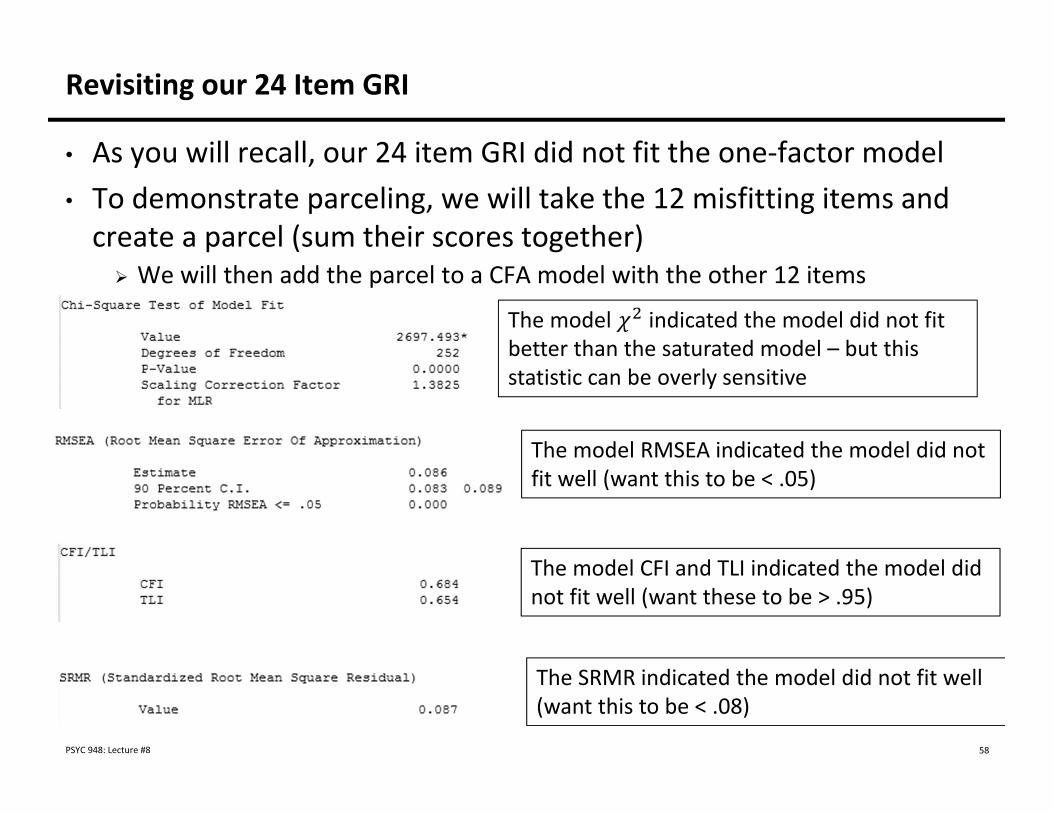
Revisiting our 24 Item GRI

• As you will recall, our 24 item GRI did not fit the one‐factor model • To demonstrate parceling, we will take the 12 misfitting items and create a parcel (sum their scores together) We will then add the parcel to a CFA model with the other 12 items


The model RMSEA indicated the model did not fit well (want this to be < .05)

The model CFI and TLI indicated the model did not fit well (want these to be > .95)

The SRMR indicated the model did not fit well (want this to be < .08)

The model indicated the model did not fit better than the saturated model – but this statistic can be overly sensitive

The 12 Item GRI Plus the Parcel of Bad Items

• The syntax:

• The model fit statistics (adequate model fit):

• Note: 12 item GRI had RMSEA of .045


How Parceling Hides Poor Model Fit

• The item parcel hides poor model fit by using a numbers game to its advantage

• Model with 24 items had 300 elements in saturated covariance matrix (but 48 parameters for that matrix)

• Model with 12 items plus parcel (12 “items”) had 91 elements in saturated covariance matrix (and 26 parameters)

• The relative ratio of parameters to saturated covariances makes the parcel hide the fit issues Especially when the remainder of the items fit well already


Parceling Done Right

• To add a parcel you must first examine the fit of a one‐factor model to the items of the parcel:

• The model fit suggests a one‐factor model doesn’t fit


Why Parceling is Cheating and Why You Shouldn’t Do It

• If you didn’t check the parcel before adding it to the 12 item GRI model you would conclude 1‐factor model fit the data well If a one‐factor model fits, then what comes next is typically the use of its sum score

• The sum score from the 12 good + 1 bad (parcel) model is just the sum score from the 24 item GRI – which didn’t fit a one‐factor model The caveat: the 12+1 model sum score had an omega reliability of .516! Most of the lack of reliability comes from the estimated unique variance of the parcel

• You cannot make a good factor by cheating with a parcel!


CONCLUDING REMARKS


Wrapping Up

• Today was spent on comparing classical test theory (synonymous with sum scores) to CFA

• Understanding how CTT and CFA are related is important Many people believe that sum scores are A‐OK

They only are if they fit a 1‐factor model and have a high reliability Many people don’t think parceling involves sum scores

The label must be the problem…

• Single indicator models can be a good way to use sum scores if: The 1‐factor model fits There is a high degree of reliability We will return to this once we discuss SEM more thoroughly


Coming Up…

• Next week’s lecture: multidimensional CFA modelsMore than one factor Reliability for a total test score no longer applies (each factor is where reliability is important)

Time permitting: an introduction to Exploratory Factor Analysis Followed by a comparison of CFA and EFA And why you also shouldn’t be doing EFA

– But could explore the data better using CFA techniques


Documents

Comparing Classical Test Theory with CFA and How … · Comparing Classical Test Theory with CFA ‐and‐ How To Use Test Scores in Secondary Analyses Latent Trait Measurement and