1  

025-0998

Comparison of periodic-review inventory control policies

in a serial supply chain

Nihan Kabadayi, İstanbul University, Faculty of Business Administration, Production

Management Department, Avcılar, Istanbul, Turkiye, nihank@istanbul.edu.tr, +90 212 473

70 70 ext:18420

Timur Keskinturk, Istanbul University, Faculty of Business Administration, Quantitative

Methods Department, Avcılar,Istanbul, Turkiye, tkturk@istanbul.edu.tr, +90 212 473 70 70

ext:18245

POMS 23rd Annual Conference

Chicago, Illinois, U.S.A.

April 20 to April 23, 2012

ABSTRACT

This study aims to compare (R, S) and (R, S, Qmin) inventory control policies in a serial

supply chain. We develop a simulation based genetic algorithm (GA) in order to find the

optimal numerical "S" value that minimizes the total supply chain cost (TSCC) and compare

our results between two methods.

Keywords: inventory management, serial supply chain, simulation-based genetic algorithm

2  

1. Introduction

In today's global economy, firms need to manage their supply chains effectively, in order

to survive in the markets and gain competitive advantage in the growing markets where

customer expectations have been rising. Supply chain management aids companies reduce

their costs, represent the products in right times, right amounts and right places by

performing in better and faster conditions, thus getting the advantage against their

competitors.

Supply chain management is very different than the management of one site. The

inventory stockpiles at the multiple sites, including both incoming materials and finished

products, have complex interrelationships. Effective and efficient management of

inventory in the supply chain process has a significant impact on improving the ultimate

customer service provided to the customer. (Lee, Billington, 1992: 65)

In order to satisfy customer demand timely, firms need to hold the right amount of

inventory. While inventory can protect firms against unpredictable market conditions, can

be very costly in a supply chain. Given the primary goal of reducing system-wide cost in a

typical supply chain; it is important to take a close look at interaction between different

facilities and the impact it has on the inventory policy that should be employed by each

facility. (Simchi-Levi, Kaminsky, Simchi-Levi, 2000: 61)

The main contribution of this paper is two-fold; first, to develop the simulation part of the

solution methodology using the Microsoft Excel spreadsheet for the sake of

implementation simplicity and second, to implement (R, S, Qmin) inventory policy

developed by Keismüller et.al. (2011) in a serial supply chain and compare it with the

classic (R, S) policy. We use simulation based GA to determine “S” numerical value

which will minimize the TSCC. In this model, the TSCC consists of two cost components

which are holding and shortage costs.

3  

The remainder of the paper is organized as follows. Section 2 considers inventory control

in multi echelon systems and describes two corresponding inventory control policies

which are used in this study. In section 3, the solution methodologies are defined. In

section 4, the numerical example is presented to test the performance of those policies.

Lastly, conclusions are summarized in section 5.

2. Inventory Control in Multi echelon systems

Inventory has a significant role in a supply chain’s ability to support a firm’s competitive

strategy. If a very high level of responsiveness is required by the firm’s competitive

strategy, this can be achieved by locating large amounts of inventory close to the

customer. On the other hand, a company can use inventory to become more efficient by

reducing inventory through centralized stocking. The responsiveness that results from

more inventory and the efficiency that results from less inventory is the main trade-off

implicit in the inventory driver. (Chopra, Meindl, 2010: 26) 

Finding the best balance between such goals is often trivial, and that is why we need

inventory models. In most situations some stock is required. The two main factors are

economies of scale and uncertainties. “Economies of scale” means we need to order in

batches. Uncertainties in supply and demand together with lead- times in production and

transportation inevitably create a need for safety stocks. Organizations can reduce their

inventories without increasing other costs by using more efficient inventory control tools.

(Axsater, 2006: 2)

Multi-echelon inventory models are central to supply chain management. The multi-

echelon inventory theory began when Clark and Scarf (1960) published their seminal

paper. (Chen, 1999: 73) Clark and Scarf (1960) consider multi-echelon inventory systems

for the first time in their study and they also use simulation to evaluate corresponding

4  

dynamic inventory model. Their study is a starting point for an enormous amount of

publications on multi-echelon systems.

There are two different decision systems used in multi echelon inventory systems and

those are centralized decision system (echelon stock) and decentralized decision system

(installation stock). Decentralized decision systems only require local inventory

information, while centralized systems require centralized demand information. (Chen,

1999: 75) The centralized decision system, in which an optimal decision to send a batch

from one site to another, may depend on the inventory status at all sites and has several

disadvantages. In order to use that kind of a decision system, the firm needs to spend an

additional cost for data movement despite the advanced information technology. In

addition to this, it is difficult to derive complete general centralized policies. As a result of

this, it is more suitable to limit the degree of centralization. (Axsater, 2006: 195) On the

other hand, relatively independent organizations often control their inventory systems and

make their own replenishment decisions, since different facilities are normally situated at

locations far from each other in a supply chain. (Petrovic, Roy, Petrovic, 1998: 302-303)

(Axsater, 2006: 195) Decentralized decision system does not require any information

about the inventory situation at other sites and it is not necessary to explicitly keep track

of the stocks at the downstream installations. These are the obvious advantages of this

type of decision systems. (Axsater, Rosling, 1993: 1274)

It is natural to think of the physical stock on hand when talking about the stock situation.

However, stock on hand cannot be the sole determinant in ordering decision. The

outstanding orders that have not yet been delivered should also be included in the

equation. Therefore, the stock situation is characterized by the inventory position in

inventory control.

 

Inve

Inve

and

poin

(Nah

cons

2

This

shar

revi

“S”,

disa

syst

Pete

entory posit

entory contr

continuous

nts in time,

hmias, 200

sidered.

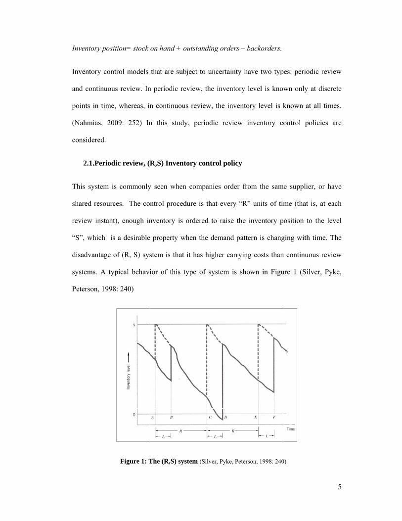
2.1.Periodi

s system is

red resource

ew instant)

, which is

advantage o

tems. A typ

erson, 1998:

tion= stock

rol models

s review. In

whereas, in

09: 252) In

ic review, (R

commonly

es. The con

), enough in

a desirable

f (R, S) sys

pical behavi

: 240)

Figure 1: T

on hand + o

that are sub

n periodic re

n continuou

n this stud

R,S) Inven

y seen when

ntrol proced

nventory is

property w

stem is that

ior of this

The (R,S) sy

outstanding

bject to unc

eview, the

us review, t

dy, periodic

tory contro

n companie

dure is that

ordered to

when the de

t it has high

type of sys

ystem (Silver

g orders – b

certainty ha

inventory l

the inventor

c review in

ol policy

es order fro

t every “R”

o raise the i

emand patte

her carrying

stem is sho

, Pyke, Peters

backorders.

ave two typ

evel is kno

ry level is k

nventory c

om the sam

” units of tim

inventory p

ern is chang

g costs than

wn in Figu

on, 1998: 240

pes: periodic

wn only at

known at a

ontrol poli

me supplier,

me (that is,

position to t

ging with ti

n continuous

ure 1 (Silve

0)

5

c review

discrete

all times.

icies are

or have

, at each

the level

me. The

s review

er, Pyke,

6  

‐‐‐‐‐‐‐‐   Inventory position

Net stock or both the inventory position and the net stock (if they are equal) 

Notes: Orders placed at times A,C and E, arrive at times B,D, and F respectively 

Most of the time, “R” and “S”, two decision variables, are not independent, that is, the

best value of “R” depends on the “S” value, and vice versa. Assuming that “R” has been

predetermined without knowledge of the “S” value is still quite reasonable for practical

purposes when dealing with B items. (Silver, Pyke, Peterson, 1998: 278) In this study, we

assume that the value of “R” is predetermined.

2.2.(R, S, Qmin) Inventory control policy

This simple periodic review policy, called (R, S, Qmin) is proposed by Keismüller et.al.(

2011). In this policy, the inventory position is monitored every “R” units of time and if the

inventory position is above the level “S”, then no order is placed. In case the inventory

position is below the level “S", an amount of order is placed which equals or exceeds Qmin

(minimum order size). An amount larger than Qmin is ordered if the minimal order size

Qmin is not sufficient to raise the inventory position up to level S. This policy is a special

case of (R, s, t, Qmin) policy which is developed by Zhou et.al. (2007) where s=S−Qmin and

t=S−1. (Keismüller, Kok, Dabia, 2011: 281)

 

F

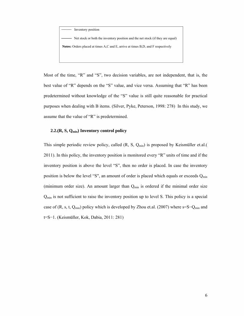
If th

case

case

leve

poli

Kies

effic

deve

solu

poli

3. S

Gen

natu

(Cha

igure 2: The

he demand

e of small va

e, the (R, S

el S. For lar

cy is equal

smüller et. a

cient cost p

eloped by

utions than (

cy ) , it is st

Solution M

3.1.Gen

netic algorit

ural selectio

ambers, 19

e (R,S,Qmin)

is always l

alues of Qm

, Qmin) poli

rge values

to an (R, s,

al. (2011) p

erformance

Zhou et.al.

(R, s, t, Qm

till practical

Methodology

netic Algori

thm (GA) i

on and gene

995: 1) The

policy (lead

larger than

min, then the

icy is simila

of Qmin the

Qmin) polic

prove that th

e, which is c

. (2007). A

min ) policy in

l with its co

y

ithm

is a mathem

etic recombi

e original m

d time equal

the minimu

order const

ar to a base

e parameter

y with a re-

he proposed

close to the

Although th

n terms of t

omputationa

matical sear

ination whi

motivation

l to zero) (Ke

um order q

traint is not

e-stock leve

r S function

-order level

d policy is s

more soph

he proposed

the cost ( s

al simplicity

rch techniq

ich is firstly

for the GA

eismüller, Ko

quantity, wh

restrictive a

el policy (R

ns as a reor

s.

imple to co

histicated tw

d policy ca

ince it is a

y.

que based o

y proposed

A approach

k, Dabia, 201

hich may ha

anymore an

R,S) with ba

rder level o

mpute and

wo-paramete

annot deriv

special cas

on the princ

by Holland

h was a bi

7

1: 281)

appen in

nd in that

ase-stock

only, the

it has an

er policy

ve better

e of that

ciples of

d (1975).

iological

8  

analogy. In the selective breeding of plants or animals, for example, offspring that have

certain desirable characteristics are sought — characteristics that are determined at the

genetic level by the way the parents’ chromosomes are combined. In the case of GAs, a

population of strings is used, and these strings are often referred to in the GA literature as

chromosomes, while the decision variables within a solution (chromosome) are genes. The

recombination of strings is carried out using simple analogies of genetic crossover and

mutation, and the search is guided by the results of evaluating the objective function (f)

for each string in the population. Based on this evaluation, strings that have higher fitness

(i.e., represent better solutions) can be identified, and these are given more opportunity to

breed. (Glover, Kochenberger, 2003: 58)

The GA search starts with the creation of a random initial population of N individuals that

might be potential solutions to the problem. Then, these individuals are evaluated for their

so-called fitnesses, i.e. of their corresponding objective function values. A mating pool of

size N is created by selecting individuals with higher fitness scores. This created

population is allowed to evolve in successive generations through the following steps:

(Marseguerra, Zio, Podofillini, 2002: 158)

1. Selection of a pair of individuals as parents;

2. Crossover of the parents, with generation of two children;

3. Replacement in the population, so as to maintain the population number N constant;

4. Genetic mutation.

The genetic operators of crossover and mutation are applied at this stage in a probabilistic

manner which results in some individuals from the mating pool to reproduce. (Chambers,

1995: 1) In general, the parent selection is fitness proportional and the survivor selection

 

is a

and

for

criti

GAs

neig

a ter

fitne

stop

Sim

exis

and

opti

Xie,

Figu

Sim

succ

generation

the mutatio

various par

ical process

s are stoch

ghborhood s

rmination c

ess evaluati

p when this

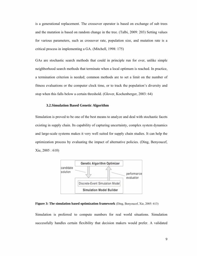
3.2.Sim

mulation is p

sting in supp

large-scale

mization pr

, 2005 : 610

ure 3: The si

mulation is

cessfully ha

al replacem

on is based

rameters, su

in impleme

astic search

search meth

criterion is

ions or the

falls below

mulation Ba

roved to be

ply chain. It

systems m

rocess by e

0)

imulation ba

preferred 

andles certa

ment. The cr

on random

uch as cros

enting a GA

h methods

hods that ter

needed; co

computer c

a certain th

ased Geneti

e one of the

ts capability

makes it very

evaluating th

ased optimiz

to comput

ain flexibili

rossover op

change in t

ssover rate,

A. (Mitchell

that could

rminate whe

ommon met

clock time,

hreshold. (G

ic Algorithm

best means

y of capturin

y well suite

he impact o

zation fram

te numbers

ity that dec

perator is ba

the tree. (Ta

, population

, 1998: 175

in principl

en a local op

hods are to

or to track

Glover, Koch

m

s to analyze

ng uncertain

d for supply

of alternativ

ework (Ding

s for real

cision make

ased on exc

albi, 2009:

n size, and

)

le run for e

ptimum is r

o set a limit

the populat

henberger, 2

and deal w

nty, comple

y chain stud

ve policies.

g, Benyoucef,

world situ

ers would p

change of s

203) Settin

mutation r

ever, unlike

reached. In p

t on the nu

tion’s diver

2003: 64)

with stochast

ex system d

dies. It can

(Ding, Ben

Xie, 2005: 61

uations. Sim

prefer. A v

9

sub trees

ng values

rate is a

e simple

practice,

umber of

rsity and

tic facets

dynamics

help the

nyoucef,

13)

mulation

validated

10  

simulation has a better chance of being accepted by end users compared to complicated

models. (Kapuscinski, Tayur, 1999: 11)

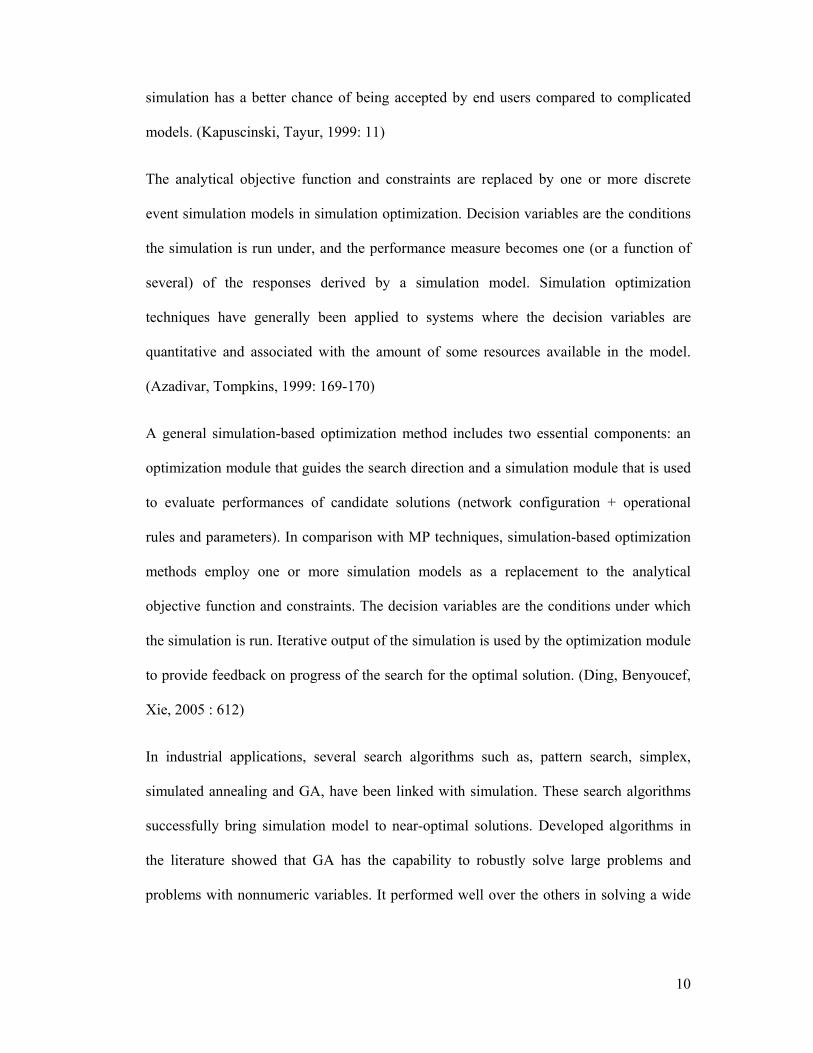
The analytical objective function and constraints are replaced by one or more discrete

event simulation models in simulation optimization. Decision variables are the conditions

the simulation is run under, and the performance measure becomes one (or a function of

several) of the responses derived by a simulation model. Simulation optimization

techniques have generally been applied to systems where the decision variables are

quantitative and associated with the amount of some resources available in the model.

(Azadivar, Tompkins, 1999: 169-170)

A general simulation-based optimization method includes two essential components: an

optimization module that guides the search direction and a simulation module that is used

to evaluate performances of candidate solutions (network configuration + operational

rules and parameters). In comparison with MP techniques, simulation-based optimization

methods employ one or more simulation models as a replacement to the analytical

objective function and constraints. The decision variables are the conditions under which

the simulation is run. Iterative output of the simulation is used by the optimization module

to provide feedback on progress of the search for the optimal solution. (Ding, Benyoucef,

Xie, 2005 : 612)

In industrial applications, several search algorithms such as, pattern search, simplex,

simulated annealing and GA, have been linked with simulation. These search algorithms

successfully bring simulation model to near-optimal solutions. Developed algorithms in

the literature showed that GA has the capability to robustly solve large problems and

problems with nonnumeric variables. It performed well over the others in solving a wide

11  

variety of simulation problems. (Ding, Benyoucef, Xie, 2005: 612) Thus, in this study we

will consider these systems as a combination of GA and simulation.

4. Numerical Example

4.1.The Model

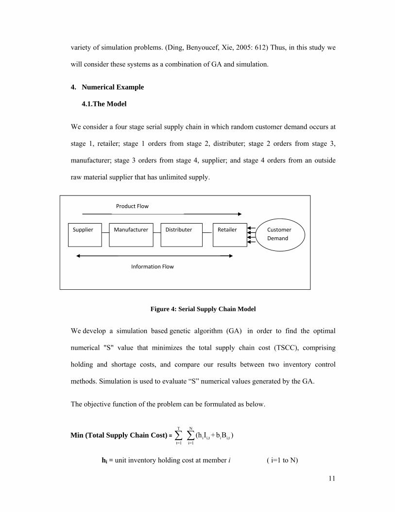
We consider a four stage serial supply chain in which random customer demand occurs at

stage 1, retailer; stage 1 orders from stage 2, distributer; stage 2 orders from stage 3,

manufacturer; stage 3 orders from stage 4, supplier; and stage 4 orders from an outside

raw material supplier that has unlimited supply.

Figure 4: Serial Supply Chain Model

We develop a simulation based genetic algorithm (GA) in order to find the optimal

numerical "S" value that minimizes the total supply chain cost (TSCC), comprising

holding and shortage costs, and compare our results between two inventory control

methods. Simulation is used to evaluate “S” numerical values generated by the GA.

The objective function of the problem can be formulated as below.

       Min (Total Supply Chain Cost) = T N

i i,t i i,tt=1 i=1

(h I + b B )  

hi = unit inventory holding cost at member i ( i=1 to N)

RetailerSupplier  Manufacturer  Distributer Customer    

Demand 

Product Flow         

Information Flow

12  

Ii,t = the quantity of on hand inventory at member i ( i=1 to N)

bi = unit shortage cost at member i ( i=1 to N)

Bi,t = the quantity of backordered inventory at member i ( i=1 to N)

Li, = replenishment lead time with respect to member i ( i=1 to N)

Di,t= demand per unit time at member i ( i=1 to N)

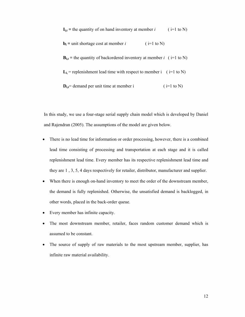
In this study, we use a four-stage serial supply chain model which is developed by Daniel

and Rajendran (2005). The assumptions of the model are given below.

There is no lead time for information or order processing, however, there is a combined

lead time consisting of processing and transportation at each stage and it is called

replenishment lead time. Every member has its respective replenishment lead time and

they are 1 , 3, 5, 4 days respectively for retailer, distributor, manufacturer and supplier.

When there is enough on-hand inventory to meet the order of the downstream member,

the demand is fully replenished. Otherwise, the unsatisfied demand is backlogged, in

other words, placed in the back-order queue.

Every member has infinite capacity.

The most downstream member, retailer, faces random customer demand which is

assumed to be constant.

The source of supply of raw materials to the most upstream member, supplier, has

infinite raw material availability.

13  

4.2.Application of the inventory control policies

We aim to observe different impacts of the relative inventory control policies in terms of

cost reduction on a specific serial supply chain model.

(R,S) inventory control policy application

Inventory level at every member is periodically monitored and if the relative inventory

position falls below the pre-specified “S” level, a replenishment order is placed for a

quantity that will bring the inventory position back to the pre-specified “S” level. Base-

stock level at every member in the supply chain takes integer values.

(R, S, Qmin) inventory control policy application

In this policy, the inventory position is monitored periodically and if the inventory

position is above the level “S”, then no order is placed. In case the inventory position is

below the level “S", an amount of order is placed which equals or exceeds Qmin (minimum

order size). An amount larger than Qmin is ordered if the minimal order size Qmin is not

sufficient to raise the inventory position up to level S.

Since (R,S,Qmin) policy differs most from the order-up-to policy (R,S) or fixed order size

policy (R,s,Q) when the numerical values of Qmin is close to the mean period demand, a

non-dimensional parameter, m=Qmin/ E [D], is introduced. In our study, we assume that

Qmin value is predetermined and it is 38 for all supply chain members while m=0.95.

4.3.Proposed Solution Methodology

Simulation-based GA is used as an experimental method to evaluate the models

performance. The supply chain simulation is run for given customer demands generated

from a uniform distribution for a specified run length over which the statistic TSCC is

collected. Random customer demand is generated uniformly within the range [20, 60] per

 

unit

TSC

The

MA

whic

gene

com

aver

orde

A m

valu

data

chro

Chr

This

set o

time. Sim

CC is noted.

GAtool in

ATLAB and

ch are gen

eration are

mpete. Addit

rage of the

er to avoid c

macro is dev

ue. Thus, GA

a and the

omosome, is

romosome re

s study uses

of “S” value

mulation exp

.

MATLAB

d Microsoft

nerated by

forced to l

tionally, we

objective fu

computation

veloped in E

A derives th

output dat

s sent to GA

epresentatio

s gene-wise

es represent

periments a

Figu

B 7 is used t

Excel in o

GA and w

eave the po

e derive 100

function (TS

nal errors th

Excel to cal

he “S” value

ta of the s

A as an inpu

on

e chromosom

ting every m

are carried o

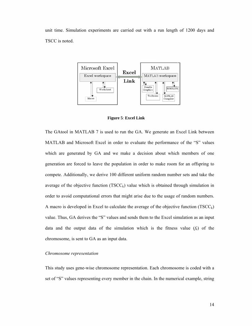
ure 5: Excel

to run the G

order to eva

we make a

opulation in

0 different u

SCCk) value

hat might a

culate the a

es and send

simulation

ut data.

me represen

member in th

out with a

Link

GA. We ge

aluate the p

decision a

n order to m

uniform ran

e which is o

arise due to

average of t

ds them to th

which is

ntation. Eac

he chain. In

run length

enerate an E

performance

about which

make room

ndom numb

obtained thr

the usage o

the objectiv

he Excel sim

the fitness

h chromoso

n the numer

h of 1200 d

Excel Link

e of the “S

h members

for an offs

ber sets and

rough simu

of random n

e function (

mulation as

value (fk)

ome is code

ical exampl

14

days and

between

” values

s of one

spring to

take the

ulation in

numbers.

(TSCCk)

an input

) of the

ed with a

le, string

15  

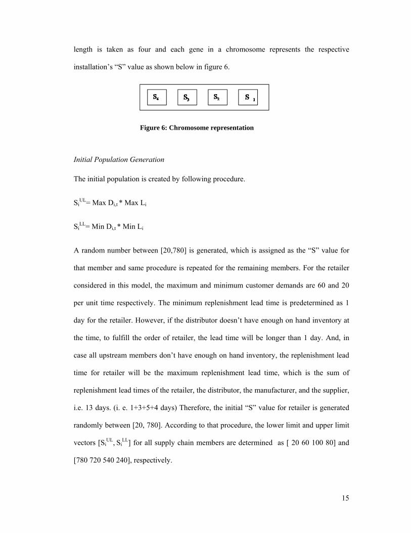
length is taken as four and each gene in a chromosome represents the respective

installation’s “S” value as shown below in figure 6.

Figure 6: Chromosome representation

Initial Population Generation

The initial population is created by following procedure.

SiUL= Max Di,t * Max Li

SiLL= Min Di,t * Min Li

A random number between [20,780] is generated, which is assigned as the “S” value for

that member and same procedure is repeated for the remaining members. For the retailer

considered in this model, the maximum and minimum customer demands are 60 and 20

per unit time respectively. The minimum replenishment lead time is predetermined as 1

day for the retailer. However, if the distributor doesn’t have enough on hand inventory at

the time, to fulfill the order of retailer, the lead time will be longer than 1 day. And, in

case all upstream members don’t have enough on hand inventory, the replenishment lead

time for retailer will be the maximum replenishment lead time, which is the sum of

replenishment lead times of the retailer, the distributor, the manufacturer, and the supplier,

i.e. 13 days. (i. e. 1+3+5+4 days) Therefore, the initial “S” value for retailer is generated

randomly between [20, 780]. According to that procedure, the lower limit and upper limit

vectors [SiUL, Si

LL] for all supply chain members are determined as [ 20 60 100 80] and

[780 720 540 240], respectively.

16  

Selection

In this study, we use the roulette-wheel selection procedure. In roulette selection process,

chromosomes are grouped together based on their fitness function values. First, MATLAB

sends each chromosome in the initial population over to the simulation in Microsoft Excel

via the M-file and the simulation calculates fitness values of those chromosomes. Then

those fitness values are again sent from Excel to GATOOL in MATLAB via the M-file.

Fitness values for each chromosome are summed up to reach a cumulative fitness value.

The process continues by dividing each chromosome’s fitness value by the cumulative

fitness value, thus calculating a percentage value for each chromosome. Then, those

percentages are lined up in order around a roulette wheel and the selection process starts; a

random uniform number between 0 and 1 is selected and whichever chromosome falls into

this number is selected to be passed on to the next generation.

 

Figure 7: Selection flow chart

In the next step, some random changes are made on chromosomes with the help of the

genetic operators, in order to obtain better results. Various trials are conducted when

determining which genetic operators to use in order to generate the optimum results. 

MATLAB 

GAtool 

Excel

M‐File

Simulation 

“S” value

fitness function    

value 

17  

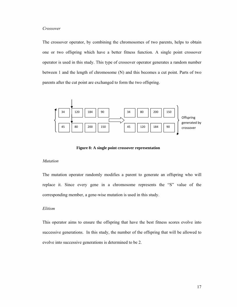
Crossover

The crossover operator, by combining the chromosomes of two parents, helps to obtain

one or two offspring which have a better fitness function. A single point crossover

operator is used in this study. This type of crossover operator generates a random number

between 1 and the length of chromosome (N) and this becomes a cut point. Parts of two

parents after the cut point are exchanged to form the two offspring.

Figure 8: A single point crossover representation

Mutation

The mutation operator randomly modifies a parent to generate an offspring who will

replace it. Since every gene in a chromosome represents the “S” value of the

corresponding member, a gene-wise mutation is used in this study.

Elitism

This operator aims to ensure the offspring that have the best fitness scores evolve into

successive generations. In this study, the number of the offspring that will be allowed to

evolve into successive generations is determined to be 2.

Offspring 

generated by 

crossover 

34  120  184  90

45  200 80  150

34 80 200 150 

45 120 184 90 

18  

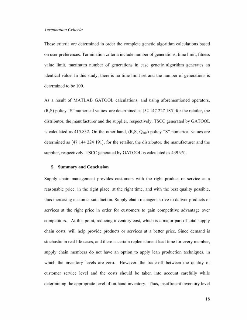
Termination Criteria

These criteria are determined in order the complete genetic algorithm calculations based

on user preferences. Termination criteria include number of generations, time limit, fitness

value limit, maximum number of generations in case genetic algorithm generates an

identical value. In this study, there is no time limit set and the number of generations is

determined to be 100.

As a result of MATLAB GATOOL calculations, and using aforementioned operators,

(R,S) policy “S” numerical values are determined as [52 147 227 185] for the retailer, the

distributor, the manufacturer and the supplier, respectively. TSCC generated by GATOOL

is calculated as 415.832. On the other hand, (R,S, Qmin) policy “S” numerical values are

determined as [47 144 224 191], for the retailer, the distributor, the manufacturer and the

supplier, respectively. TSCC generated by GATOOL is calculated as 439.951.

5. Summary and Conclusion

Supply chain management provides customers with the right product or service at a

reasonable price, in the right place, at the right time, and with the best quality possible,

thus increasing customer satisfaction. Supply chain managers strive to deliver products or

services at the right price in order for customers to gain competitive advantage over

competitors. At this point, reducing inventory cost, which is a major part of total supply

chain costs, will help provide products or services at a better price. Since demand is

stochastic in real life cases, and there is certain replenishment lead time for every member,

supply chain members do not have an option to apply lean production techniques, in

which the inventory levels are zero. However, the trade-off between the quality of

customer service level and the costs should be taken into account carefully while

determining the appropriate level of on-hand inventory. Thus, insufficient inventory level

19  

might lead to inferior customer service level and satisfaction albeit a lower product cost.

In this study, we aim to determine the optimal level of on-hand inventory in order to

minimize supply chain inventory costs. In the decision process, in order to save on time

and costs, supply chain managers should prefer a method such as simulation, which better

reflects uncertainties of real life situations. In addition to this, they can use a heuristic

optimization method, such as genetic algorithm which derives optimal solutions in a short

time period. Using a combination of those two methods, thus placing results generated by

genetic algorithm into the simulation, they can observe results in several different realistic

circumstances.

In our study, we examine the application and measure the performance of the inventory

policy (R, S, Qmin) developed by Keismüller et.al.(2011) on the four stage serial supply

chain model. This policy was considered on a single item single echelon system with

stochastic demand in a previous study. Our study extends (R, S, Qmin) inventory control

policy implementation by applying it in a multi echelon system. We develop a simulation

model using Microsoft Excel spreadsheet for the sake of implementation simplicity. This

simulation model can be used to evaluate the performance of the (R, S, Qmin) inventory

policy on various supply chain scenarios.

Afterwards, we compare the relative inventory policy with the classic (R, S) policy.

According to our experimental results, the (R, S, Qmin) policy costs slightly more than the

classic (R,S) policy, for the given scenario. However, it leads to a better customer service

level by avoiding inventory shortages. Also, (R, S, Qmin) policy is more efficient when

economies of scale exist. We use a simulation based GA to determine the “S” numerical

value which will minimize the TSCC. In this model, the TSCC consists of two cost

components which are holding and shortage costs. The solution methodology used in this

study is easy to implement and doesn’t require cumbersome mathematical endeavors,

20  

which makes the process practical for users who don’t have advanced level of analytical

skills.

21  

6. References

Axsater S., Inventory Control, Springer Science, New York, Second edition, 2006

Axsater S., Rosling K., Installation vs. Echelon Stock Control Policies for Multi-level

Inventory Control, Management Science, vol.39, no. 10, 1993, pp. 1274 -1280

Azadivar F., Tompkins G., Simulation optimization with qualitative variables and

structural model changes: A genetic algorithm approach, European Journal of

Operational Research, 113, 1999, 169-182

Chambers, J., Practical Handbook of Genetic Algorithms :Volume 2: New Frontiers,

CRC-Press; 1 edition ,1995

Chen F., On (R,NQ) policies in serial inventory systems, Tayur, S., Ganeshan, R.,

Magazine, M.J., Quantitative Models for Supply Chain Management, Kluwer Academic

Publishers, Massachusetts, 1999, pp. 73-109

Chopra S., Meindl P.; Supply Chain Management: Strategy, Planning and Operation,

Prentice-Hall Inc., New Jersey, 4th edition, 2010

Ding H., Benyoucef L., Xie X., A simulation-based multi-objective genetic algorithm

approach for networked enterprises optimization, Engineering Applications of Artificial

Intelligence, 19, 2005, pp.609-623

Kapuscinski R., Tayur S., Optimal policies and simulation-based optimization for

capacitated production inventory systems, Tayur, S., Ganeshan, R., Magazine, M.J.,

Quantitative Models for Supply Chain Management, Kluwer Academic Publishers,

Massachusetts, 1999, pp. 7-41

22  

Kiesmüller G.P., Kok A.G. de, Dabia S. ,Single item inventory control under periodic

review and a minimum order quantity, International Journal of Production Economics,

133, 2011, pp.280-285

Lee H.L., Billington C., Managing Supply Chain Inventory: Pitfalls and Opportunities,

Sloan Management Review, Spring 1992,33, pp.65-73

Marseguerra M., Zio E., Podofillini L., Condition-based maintenance optimization by

means of genetic algorithms and Monte Carlo simulation, Reliability Engineering and

System Safety, 77,2002, pp. 151–166

Nahmias S., Production and Operation Analysis, McGraw-Hill International edition,

2009,New York

Petrovic D., Roy R., Petrovic R., Modeling and simulation of a supply chain in an

uncertain environment, European Journal of Operations Research, Vol. 109, No.2, 1998,

pp. 299-309

Simchi-Levi D., Kaminsky P., Simchi-Levi E., Desingning and Managing the Supply

Chain, Irwin McGraw-Hill, 2000

Talbi El-G., Metaheuristics, John Wiley & Sons, Inc., New Jersey, 2009

Zhou,B., Zhao, Y., Katehakis, M.N., , Effective control policies for stochastic inventory

systems with a minimum order quantity, Probability in the Engineering and Informational

Sciences, 20, 2007, pp. 257-270