Course overview

Digital Image SynthesisYung-Yu Chuang9/21/2006

with slides by Mario Costa Sousa, Pat Hanrahan and Revi Ramamoorthi

Logistics

• Meeting time: 1:30pm-4:20pm, Thursday• Classroom: CSIE Room 111 • Instructor: Yung-Yu Chuang (cyy@csie.ntu.edu.tw)

• TA: Shan-Yung Yang• Webpage:

http://www.csie.ntu.edu.tw/~cyy/renderingid/password

• Forum:http://www.cmlab.csie.ntu.edu.tw/~cyy/forum/viewforum.php?f=8

• Mailing list: rendering@cmlab.csie.ntu.edu.twPlease subscribe viahttps://cmlmail.csie.ntu.edu.tw/mailman/listinfo/rendering/

Prerequisites

• C++ program experience is required.• Basic knowledge on algorithm and data

structure is essential.• Knowledge on linear algebra, probability and

compilers is a plus.• Though not required, it is recommended that

you have background knowledge on computer graphics.

Requirements (subject to change)

• 2 programming assignments (40%)• Presentation (15%) (course will alternate

between lectures and paper presentations)• Class participation (5%)• Final project (40%)

Textbook

Physically Based Rendering from Theory to Implementation, by Matt Pharr and Greg Humphreys

•Authors have a lot of experience on ray tracing

•Complete (educational) code, more concrete

•Plug-in architecture, easy for experiments and extension

•Has been used in some papers

Literate programming

• A programming paradigm proposed by Knuth when he was developing Tex.

• Programs should be written more for people’s consumption than for computers’ consumption.

• The whole book is a long literate program. That is, when you read the book, you also read a complete program.

Features

• Mix prose with source: description of the code is as important as the code itself

• Allow presenting the code to the reader in a different order than to the compiler

• Easy to make index• Traditional text comments are usually not

enough, especially for graphics• This decomposition lets us present code a few

lines at a time, making it easier to understand.• It looks more like pseudo code.

LP example@\section{Selection Sort: An Example for LP}

We use {\it selection sort} to illustrate the concept of {it literate programming}.Selection sort is one of the simplest sorting algorithms.It first find the smallest element in the array and exchange it with the element in the first position, then find the second smallest element and exchange it the element in the second position, and continue in this way until the entire array is sorted.The following code implement the procedure for selection sortassuming an external array [[a]].

<<*>>=<<external variables>>void selection_sort(int n) {

<<init local variables>>for (int i=0; i<n-1; i++) {

<<find minimum after the ith element>><<swap current and minimum>>

}}

LP example<<find minimum after the ith element>>=min=i;for (int j=i+1; j<n; j++) {

if (a[j]<a[min]) min=j;}

<<init local variables>>=int min;

@ To swap two variables, we need a temporary variable [[t]] which is declaredat the beginning of the procedure.<<init local variables>>=int t;

@ Thus, we can use [[t]] to preserve the value of [[a[min]] so that theswap operation works correctly.<<swap current and minimum>>=t=a[min]; a[min]=a[i]; a[i]=t;

<<external variables>>=int *a;

LP example (tangle)int *a;

void selection_sort(int n) {int min;

int t;

for (int i=0; i<n-1; i++) {min=i;for (int j=i+1; j<n; j++) {

if (a[j]<a[min]) min=j;}

t=a[min]; a[min]=a[i]; a[i]=t;

}}

LP example (weave)

Reference books

Reference

• SIGGRAPH proceedings• Proceedings of Eurographics Symposium on

Rendering• Eurographics proceedings

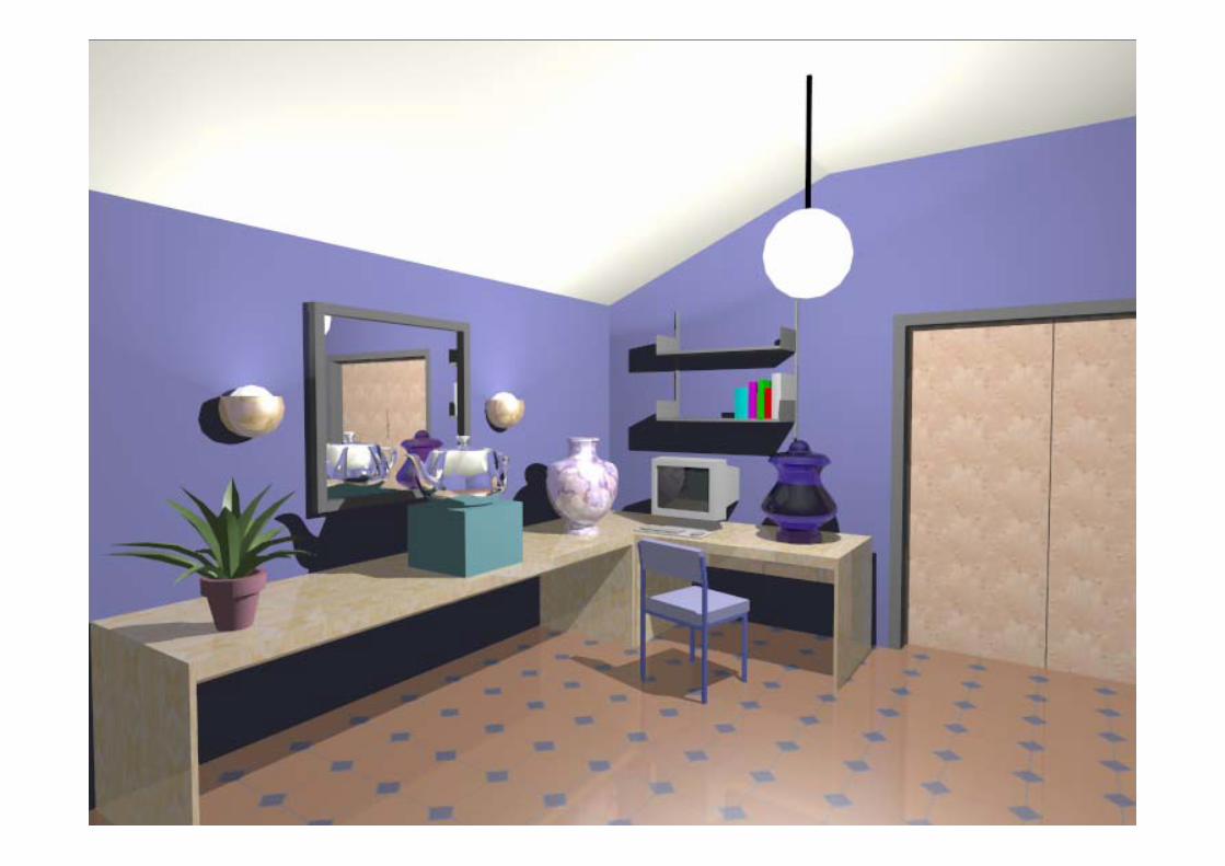
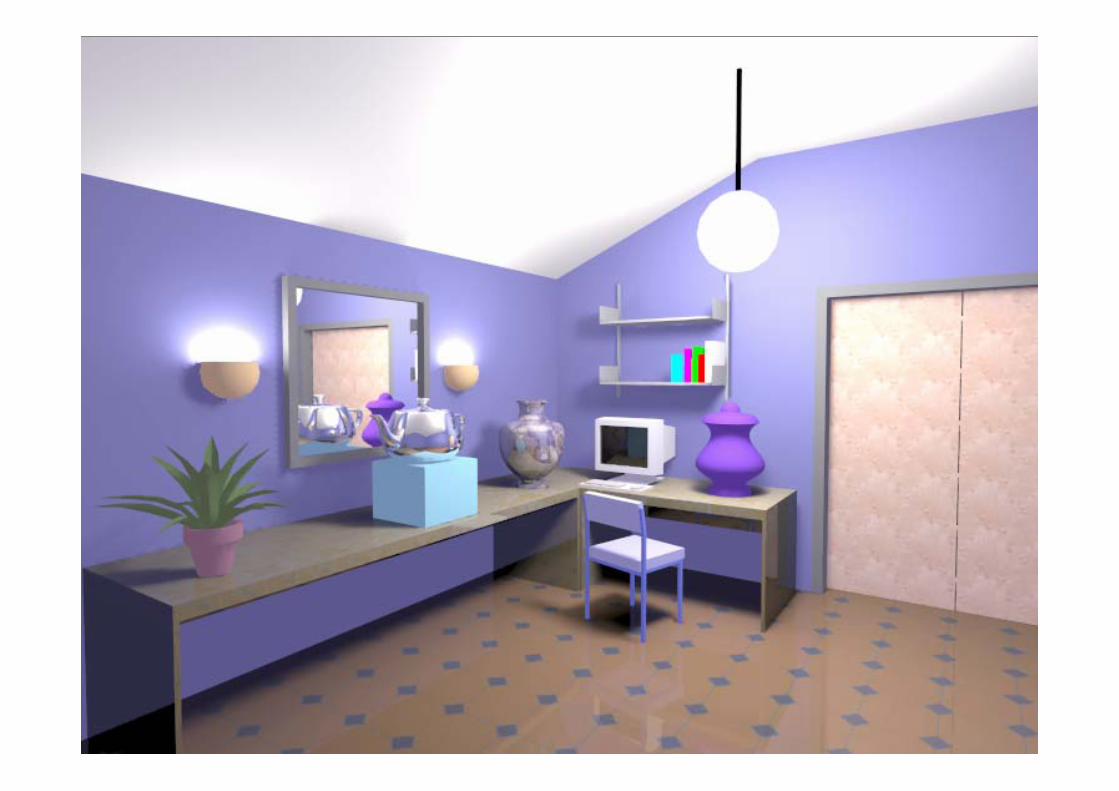
Image synthesis (Rendering)

• Create a 2D picture of a 3D world

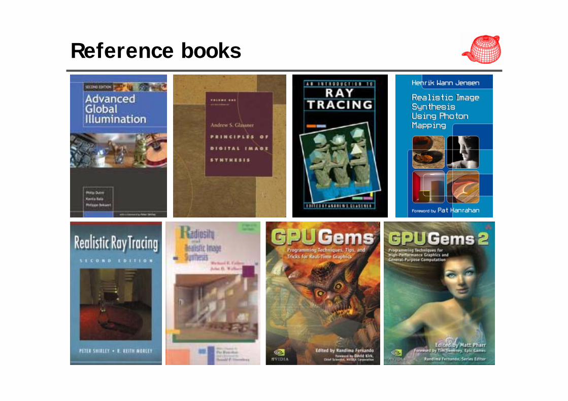
Applications

• Movies• Interactive entertainment• Industrial design• Architecture• Culture heritage

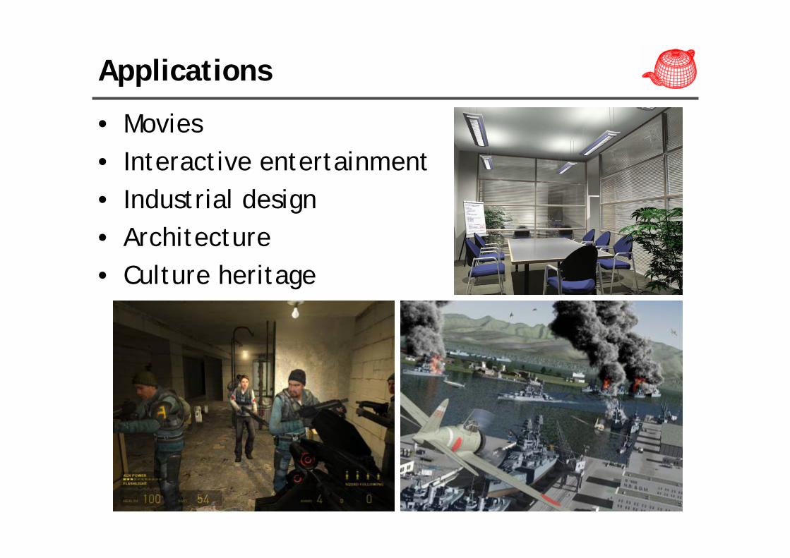
Animation production pipeline

story text treatment storyboard

voice storyreal look and feel

Animation production pipeline

layout animation

shading/lighting

modeling/articulation

rendering final touch

Computer graphics

modeling rendering

animation

The goal of this course

• Realistic rendering• First part: physically based rendering• Second part: real-time high quality rendering

Physically-based rendering

uses physics to simulate the interaction between matter and light, realism is the primary goal

• Shadows• Reflections (Mirrors)• Transparency • Interreflections• Detail (Textures…)• Complex Illumination• Realistic Materials• And many more

Realism

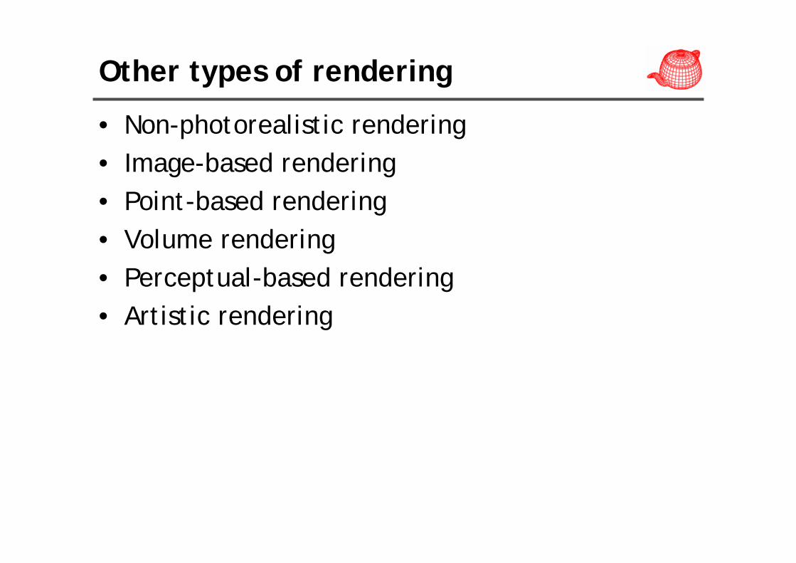
Other types of rendering

• Non-photorealistic rendering• Image-based rendering• Point-based rendering• Volume rendering• Perceptual-based rendering• Artistic rendering

Pinhole camera

Introduction to ray tracing

Ray Casting (Appel, 1968)

Ray Casting (Appel, 1968)

Ray Casting (Appel, 1968)

Ray Casting (Appel, 1968)

( ) ( )( )∑=

⋅+⋅+nls

i

nisidiaa VRkNLkIIk

1

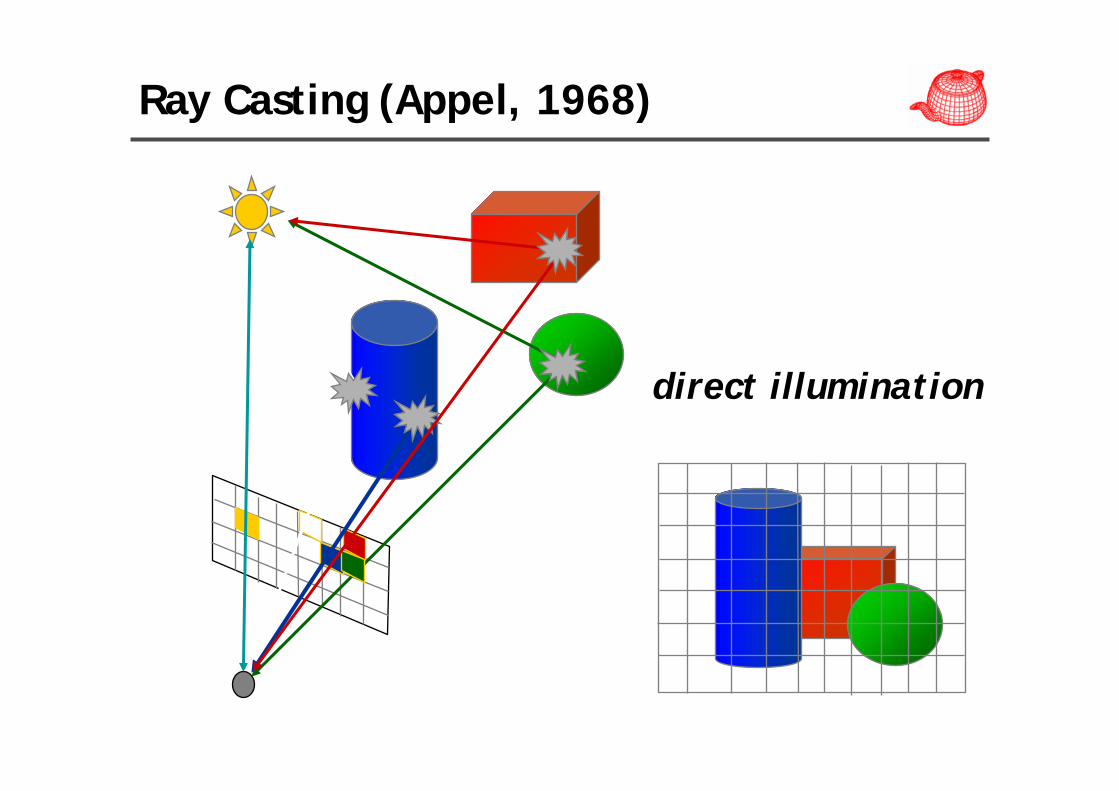
Ray Casting (Appel, 1968)

direct illumination

Whitted ray tracing algorithm

Whitted ray tracing algorithm

Shading

Ray tree

Recursive ray tracing (Whitted, 1980)

Components of a ray tracer

• Cameras• Films• Lights• Ray-object intersection• Visibility• Surface scattering• Recursive ray tracing

Minimal ray tracer

• Minimal ray tracer contest on comp.graphics, 1987

• Write the shortest Whitted-style ray tracer in C with the minimum number of tokens. The scene is consisted of spheres. (specular reflection and refraction, shadows)

• Winner: 916 tokens• Cheater: 66 tokens (hide source in a string)• Almost all entries have six modules: main, trace,

intersect-sphere, vector-normalize, vector-add, dot-product.

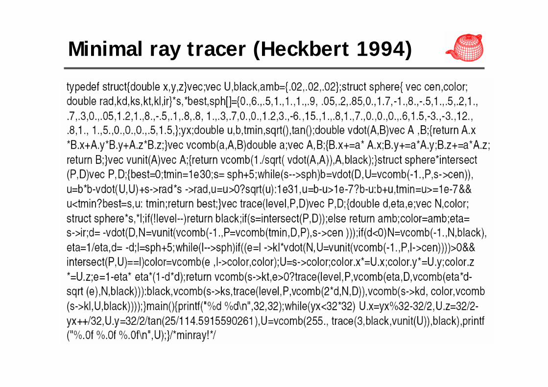
Minimal ray tracer (Heckbert 1994)

Let’s trace code

• Pretty much the same as the format of the textbook, illustrating concepts by showing working source code

• Ray tracer usually contains tricks (for efficiency, here, for reducing tokens)

• The basic frameworks are the same

Minimal ray tracer (scene description)•888 tokens

/* ray.h for test1, first test scene */#define DEPTH 3 /* max ray tree depth */#define SIZE 32 /* resolution of picture in x and y */#define AOV 25 /* total angle of view in degrees */#define NSPHERE 5 /* number of spheres */

AMBIENT = {.02, .02, .02}; /* ambient light color */

/* sphere: x y z r g b rad kd ks kt kl ir */SPHERE = {

0., 6., .5, 1., 1., 1., .9, .05, .2, .85, 0., 1.7,-1., 8., -.5, 1., .5, .2, 1., .7, .3, 0., .05, 1.2,1., 8., -.5, .1, .8, .8, 1., .3, .7, 0., 0., 1.2,3., -6., 15., 1., .8, 1., 7., 0., 0., 0., .6, 1.5,

-3., -3., 12., .8, 1., 1., 5., 0., 0., 0., .5, 1.5,};

radius

diffuse

reflection

refraction

emitting

index

Minimal ray tracer (geometry)/* minimal ray tracer, hybrid version - 888 tokens* Paul Heckbert, ucbvax!pixar!ph, 13 Jun 87* Using tricks from Darwyn Peachey and Joe Cychosz.

*/

#define TOL 1e-7#define AMBIENT vec U, black, amb#define SPHERE struct sphere {vec cen, color; \

double rad, kd, ks, kt, kl, ir} \*s, *best, sph[]

typedef struct {double x, y, z} vec;#include "ray.h"yx;double u, b, tmin, sqrt(), tan();

Minimal ray tracer (geometry utilities)double vdot(A, B)vec A, B;{ return A.x*B.x + A.y*B.y + A.z*B.z; }

vec vcomb(a, A, B) /* aA+B */double a;vec A, B;{

B.x += a*A.x;B.y += a*A.y;B.z += a*A.z;return B;

}

vec vunit(A)vec A;{ return vcomb(1./sqrt(vdot(A, A)), A, black); }

Minimal ray tracer (cameras/films)main(){printf("%d %d\n", SIZE, SIZE);while (yx<SIZE*SIZE)

U.x = yx%SIZE-SIZE/2,U.z = SIZE/2-yx++/SIZE,

/* 360/PI~=114 */U.y = SIZE/2/tan(AOV/114.5915590261),U = vcomb(255.,trace(DEPTH,black,vunit(U)),black),/* yowsa! non-portable! */printf("%.0f %.0f %.0f\n", U);

}

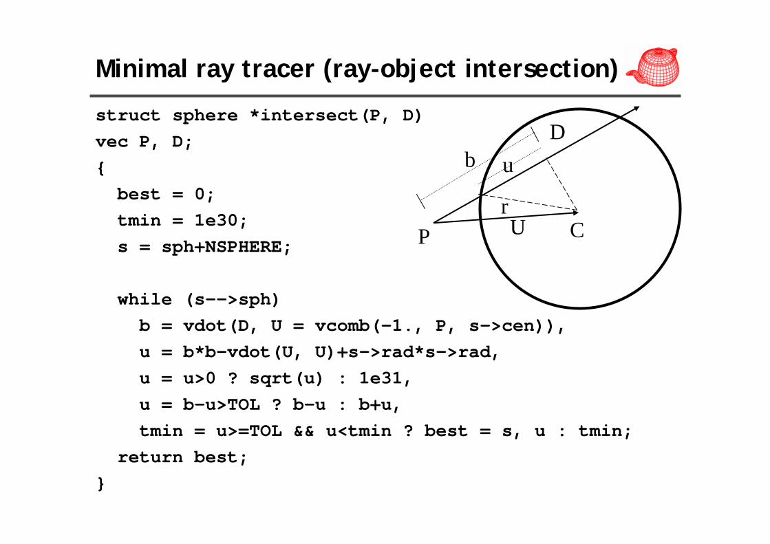
struct sphere *intersect(P, D)vec P, D;{

best = 0;tmin = 1e30;s = sph+NSPHERE;

while (s-->sph)b = vdot(D, U = vcomb(-1., P, s->cen)),u = b*b-vdot(U, U)+s->rad*s->rad,u = u>0 ? sqrt(u) : 1e31,u = b-u>TOL ? b-u : b+u,tmin = u>=TOL && u<tmin ? best = s, u : tmin;

return best;}

Minimal ray tracer (ray-object intersection)

P

D

b

C

r

U

-u

struct sphere *intersect(P, D)vec P, D;{

best = 0;tmin = 1e30;s = sph+NSPHERE;

while (s-->sph)b = vdot(D, U = vcomb(-1., P, s->cen)),u = b*b-vdot(U, U)+s->rad*s->rad,u = u>0 ? sqrt(u) : 1e31,u = b-u>TOL ? b-u : b+u,tmin = u>=TOL && u<tmin ? best = s, u : tmin;

return best;}

Minimal ray tracer (ray-object intersection)

P

D

CrU

b u

Minimal ray tracer (recursive ray tracing)vec trace(level, P, D)vec P, D;{

double d, eta, e;vec N, color;struct sphere *s, *l;

if (!level--) return black;if (s = intersect(P, D));else return amb;

color = amb;eta = s->ir;d = -vdot(D,

N = vunit(vcomb(-1.,P=vcomb(tmin,D,P),s->cen)));if (d<0) /* go into sphere */

N = vcomb(-1., N, black),eta = 1/eta, d = -d;

D

C

PN

η

N

Minimal ray tracer (recursive ray tracing)l = sph+NSPHERE;while (l-->sph)

if ((e=l->kl*vdot(N,U=vunit(vcomb(-1.,P,l->cen))))> 0 && intersect(P, U)==l)

color = vcomb(e, l->color, color);U = s->color;color.x *= U.x;color.y *= U.y;color.z *= U.z;e = 1-eta*eta*(1-d*d);/* the following is non-portable: we assume right

to left arg evaluation.(use U before call to trace, which modifies U)*/

return vcomb(s->kt,e>0 ? trace(level, P,

vcomb(eta,D,vcomb(eta*d-sqrt(e), N, black))): black,

vcomb(s->ks, trace(level, P, vcomb(2*d, N, D)),vcomb(s->kd, color, vcomb(s->kl, U, black))));

}

Reflection

R=d-2(N∙d)N

Minimal ray tracer (recursive ray tracing)l = sph+NSPHERE;while (l-->sph)

if ((e=l->kl*vdot(N,U=vunit(vcomb(-1.,P,l->cen))))> 0 && intersect(P, U)==l)

color = vcomb(e, l->color, color);U = s->color;color.x *= U.x;color.y *= U.y;color.z *= U.z;e = 1-eta*eta*(1-d*d);/* the following is non-portable: we assume right

to left arg evaluation.(use U before call to trace, which modifies U)*/

return vcomb(s->kt,e>0 ? trace(level, P,

vcomb(eta,D,vcomb(eta*d-sqrt(e), N, black))): black,

vcomb(s->ks, trace(level, P, vcomb(2*d, N, D)),vcomb(s->kd, color, vcomb(s->kl, U, black))));

}

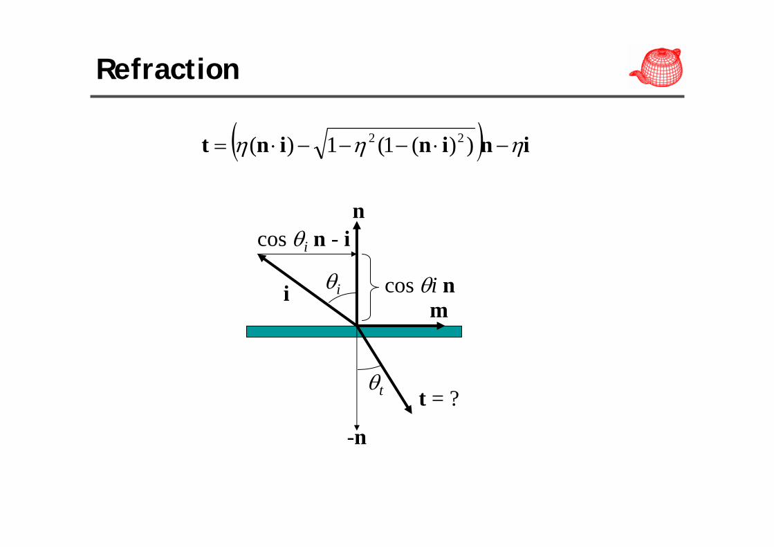
Refraction

( ) ininint ηηη −⋅−−−⋅= ))(1(1)( 22

cos θi n - i

i

n

-n

θi

θt t = ?

mcos θi n

That’s it?

• In this course, we will study how state-of-art ray tracers work.

Issues

• Better Lighting + Forward Tracing• Texture Mapping• Sampling• Modeling• Materials• Motion Blur, Depth of Field, Blurry

Reflection/Refraction– Distributed Ray-Tracing

• Improving Image Quality• Acceleration Techniques (better structure,

faster convergence)

Complex lighting

Complex lighting

Refraction/dispersion

Caustics

Realistic materials

Translucent objects

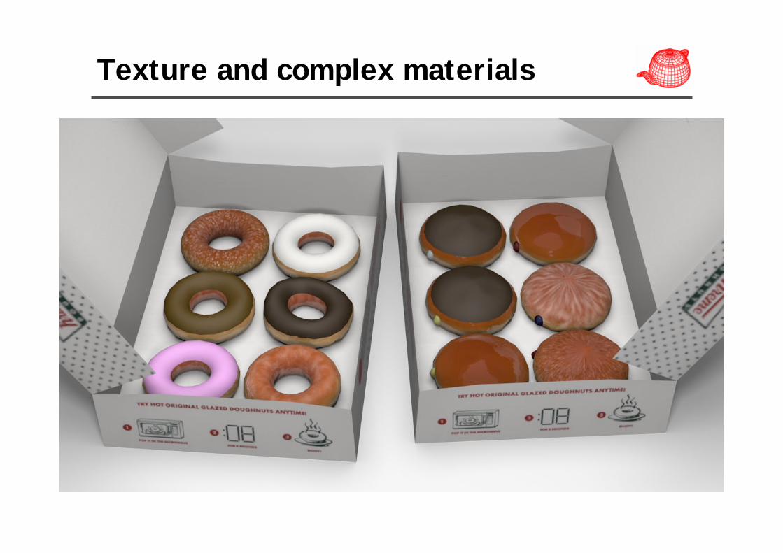
Texture and complex materials

Even more complex materials

What else you can learn

• Literate programming• Lex and yacc• Object-oriented design• Code optimization tricks• Monte Carlo method• Sampling and reconstruction• Wavelet transform• Spherical harmonics

Carousel at Night by Alex Kozlowski@UCSD

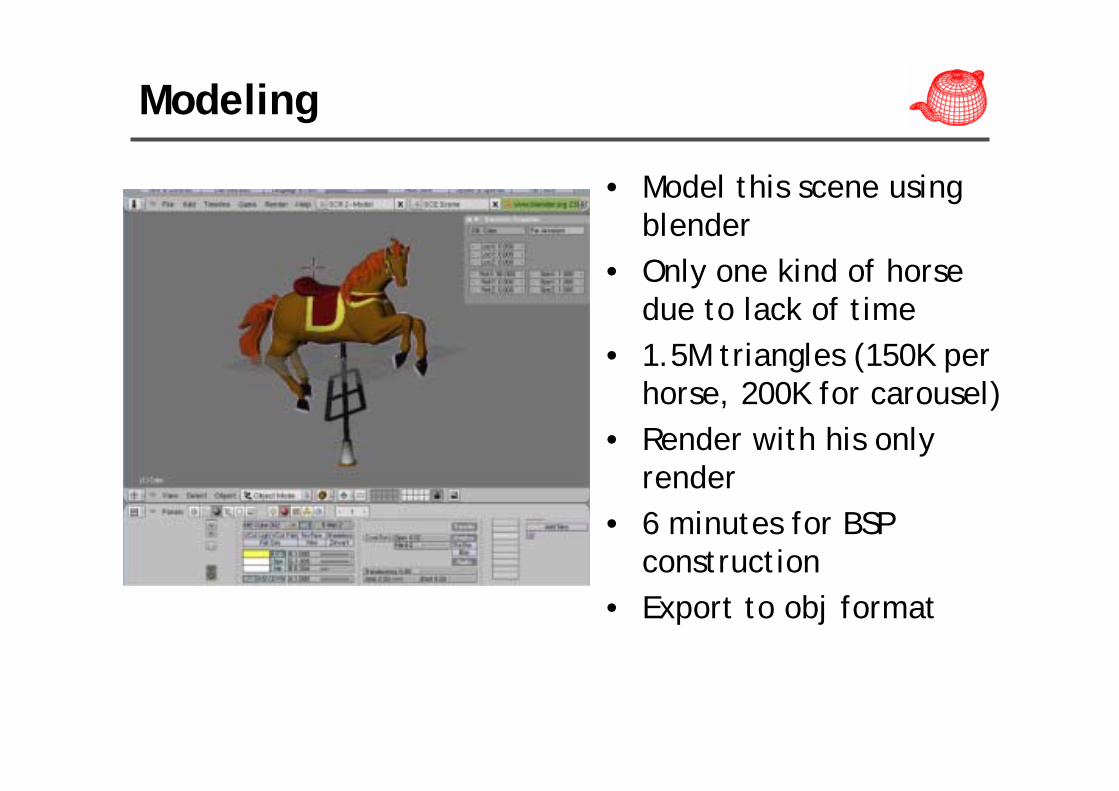
Modeling

• Model this scene using blender

• Only one kind of horse due to lack of time

• 1.5M triangles (150K per horse, 200K for carousel)

• Render with his only render

• 6 minutes for BSP construction

• Export to obj format

Soft shadows

• stratified sampling of the spherical area lights

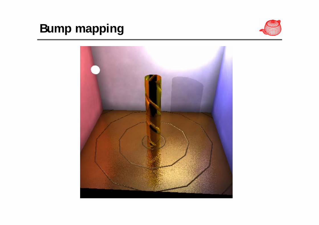
Bump mapping

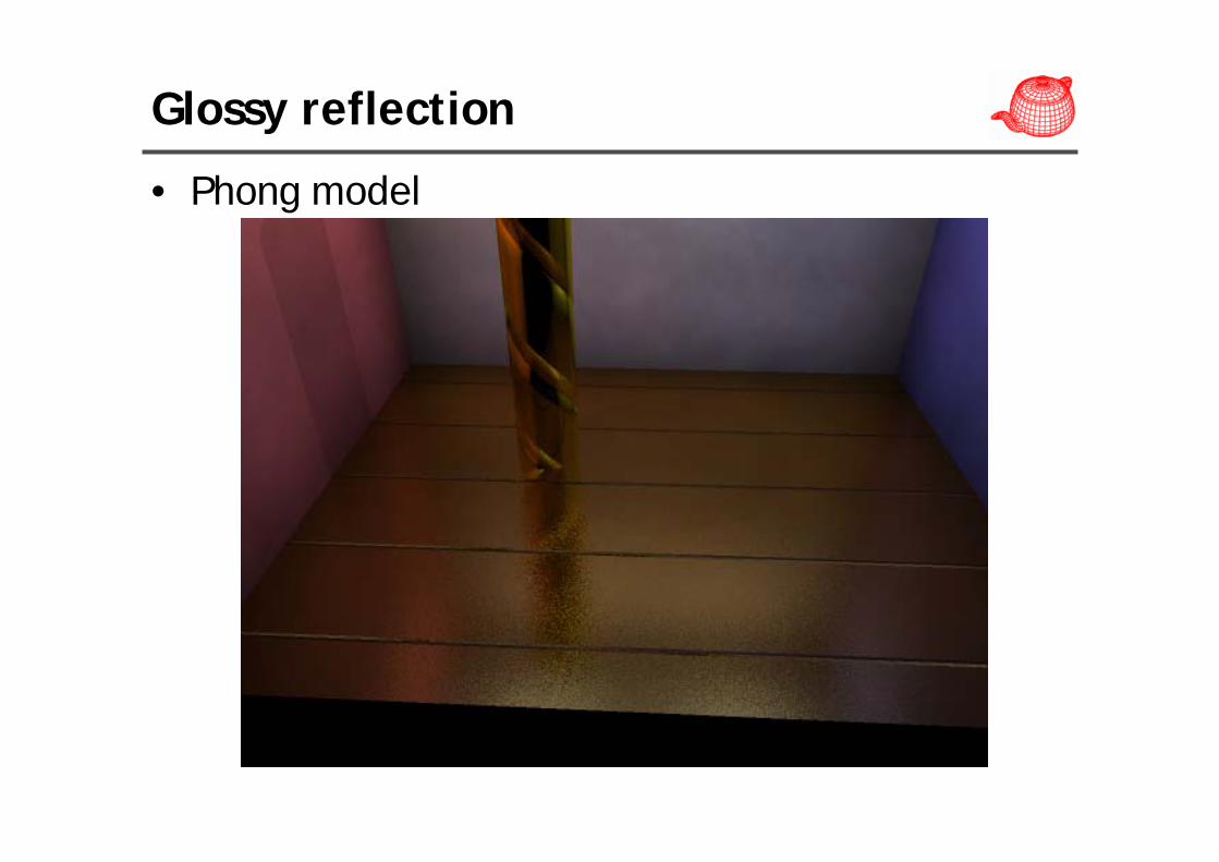
Glossy reflection

• Phong model

Perlin texture

Depth of field/supersampling

• circular lens with 16 samples per pixel, stratified sampling for both the pixel locations and the lens

Tone mapping

• 500 spherical lights, 3 Watts per light

Tone mapping

• 500 spherical lights, 3 Watts per light

The Caterpillar by T. Vaish & S. Budhiraja@Stanford

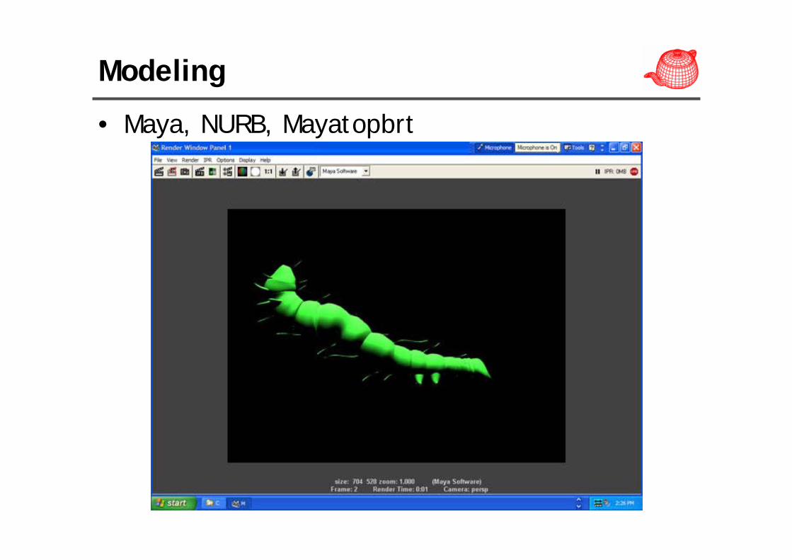
Modeling

• Maya, NURB, Mayatopbrt

Modeling

• Maya, NURB, Mayatopbrt

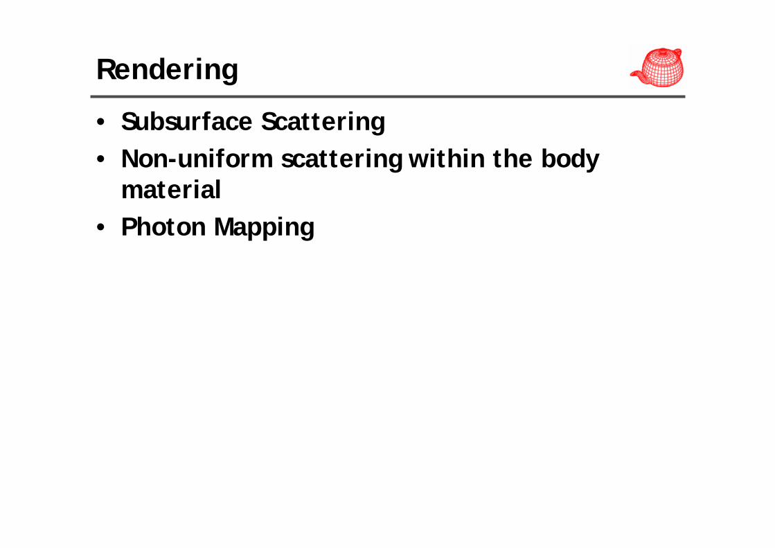
Rendering

• Subsurface Scattering• Non-uniform scattering within the body

material• Photon Mapping

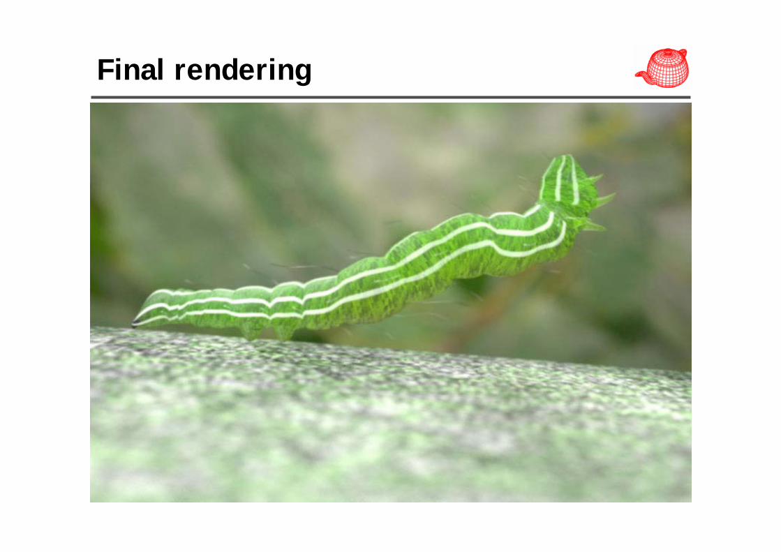
Final rendering

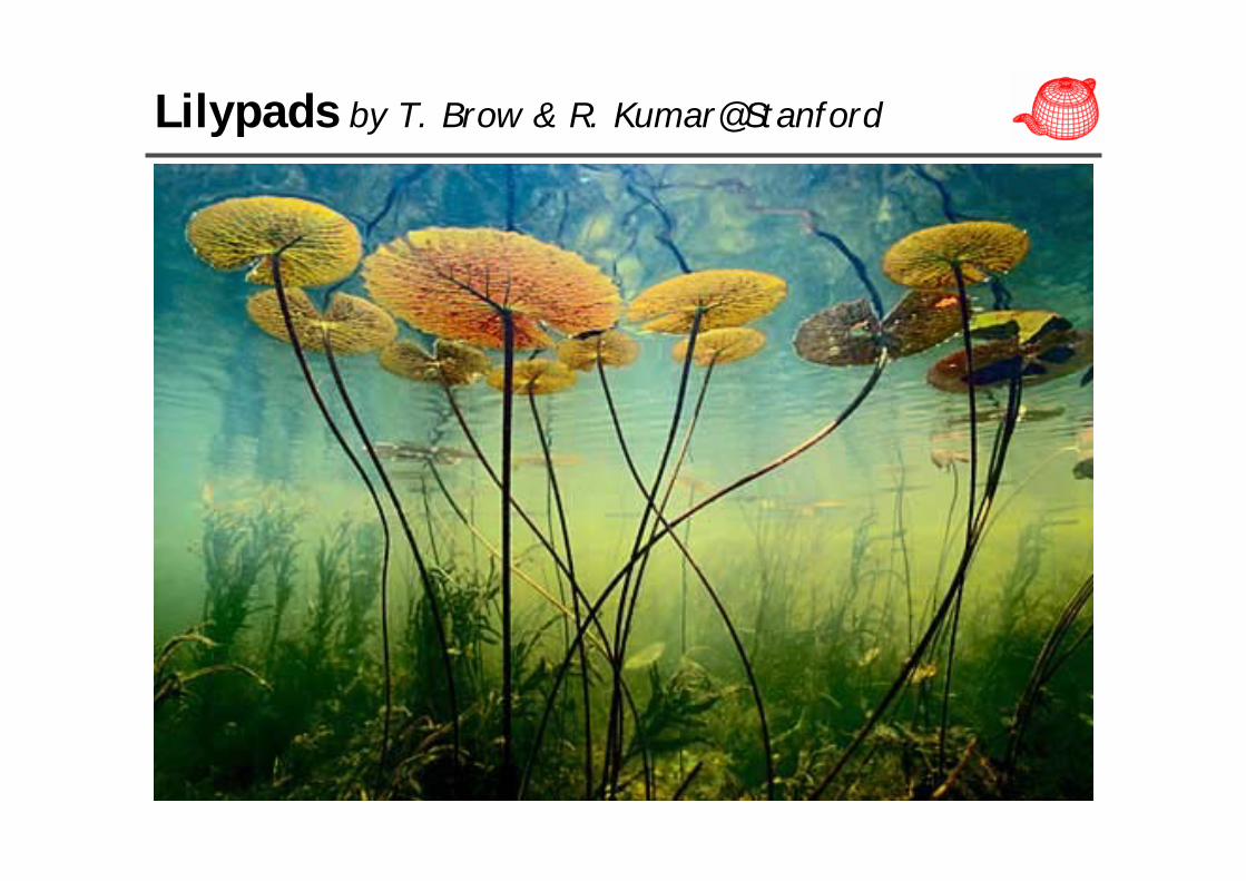
Lilypads by T. Brow & R. Kumar@Stanford

Modeling

• Mathematica

Modeling

Rendering

• Subsurface Scattering• Photon Mapping

Final rendering

Homework #0

• Download and install pbrt• Set it up in a debugger environment so that you

can trace the code• Run several examples• Optionally, create your own scene