孙昌璞

http://power.itp.ac.cn/~suncp/quantum.htm

中国科学院理论物理研究所

长春大学，长春2010年8月

量子态操纵的基础物理问题

第3讲：基于(反)Zeno效应的量子操纵

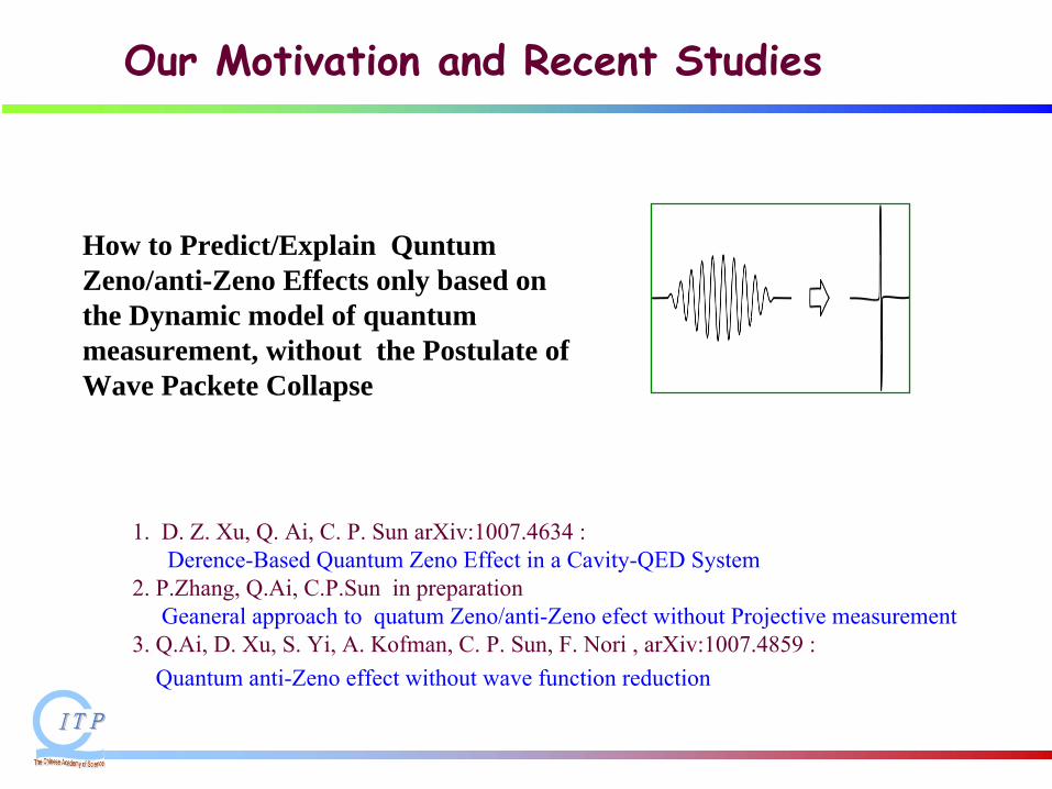
Our Motivation and Recent Studies

1. D. Z. Xu, Q. Ai, C. P. Sun arXiv:1007.4634 : Derence-Based Quantum Zeno Effect in a Cavity-QED System

2. P.Zhang, Q.Ai, C.P.Sun in preparation Geaneral approach to quatum Zeno/anti-Zeno efect without Projective measurement

3.

Q.Ai, D. Xu, S.

Yi, A. Kofman, C. P. Sun, F.

Nori , arXiv:1007.4859 :Quantum anti-Zeno effect without wave function reduction

How to Predict/Explain Quntum Zeno/anti-Zeno Effects only based on the Dynamic model of quantum measurement, without the Postulate of Wave Packete Collapse

1. Quantum Zeno effect (QZE)

"proves" projection measurement？

2 . No Projection in reality for QZE: Revisiting existing experiments

3. Anti-QZE for open quantum system in dynamics

Content

Other relevant papers

Quantum Zeno Effect: 1. L. A. Khalhin, JETP Lett. 8, 65 (1968).2. B. Misra, E. C. G. Sudarshan, J. Math. Phys. 18, 756 (1977).

Quantum Anti-Zeno Effect:3. A. M. Lane, Phys. Lett. A 99, 359 (1983).4. A. G. Kofman & G. Kurizki, Nature 405, 546 (2000).5. P. Facchi, H. Nakazato, and S. Pascazio, Phys. Rev. Lett. 86, 2699 (2001).

Quantum (Anti-)Zeno and Rotating-Wave Approximation:6. H. Zheng, S. Y. Zhu, M. S. Zubairy, Phys. Rev. Lett. 101, 200404 (2008).7. Q. Ai, Y. Li, H. Zheng, C. P. Sun, Phys. Rev. A 81, 042116 (2010).8. Q. Ai, J. Q. Liao, C. P. Sun, arXiv:1003.4587 (2010).

Dynamic Approach for Quantum Zeno Effect:9. W. M. Itano, D. J. Heinzen, J. J. Bollinger, D. J. Wineland, Phys. Rev. A 41, 2295 (1990).

10. L. E. Ballentine, Phys. Rev. A 43, 5165 (1991).11. C. P. Sun, in Quantum Classical Correspondence: The 4th Drexel Symposium on

Quantum Nonintegrability, 1994, edited by D. H. Feng and B. L. Hu (International Press, Cambridge, MA), p. 99. For a review, see C. P. Sun, X. X. Yi and X. J. Liu, Fortschr. Phys. 43, 585 (1995).

Dynamic Approach for Quantum Anti-Zeno Effect:12. Q. Ai, D. Z. Xu, A. G. Kofman, C. P. Sun, F. Nori, arXiv:1007.4859 (2010).Review on Quantum Zeno Effect:13. K. Koshinoa and A. Shimizu, Phys. Rep. 412, 191 (2005).

1. Quantum Zeno effect (QZE)

"proves" projection measurement？

2 . No Projection in reality for QZE: Revisiting existing experiments

3. Reamrks on Foundamental problems:Two von Neumanns , two Physicses !

4. Anti-QZE for open quantum system in dynamics

Content

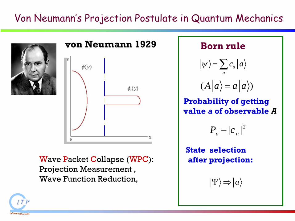
Von Neumann’s Projection Postulate in Quantum Mechanics

Probability of getting value a of observable A

2= | |a aP c

Born rule

State selectionafter projection:

aa

c aψ =∑

Wave Packet Collapse (WPC): Projection

Measurement ,

Wave Function Reduction,

( )A a a a=

aΨ ⇒

von Neumann 1929

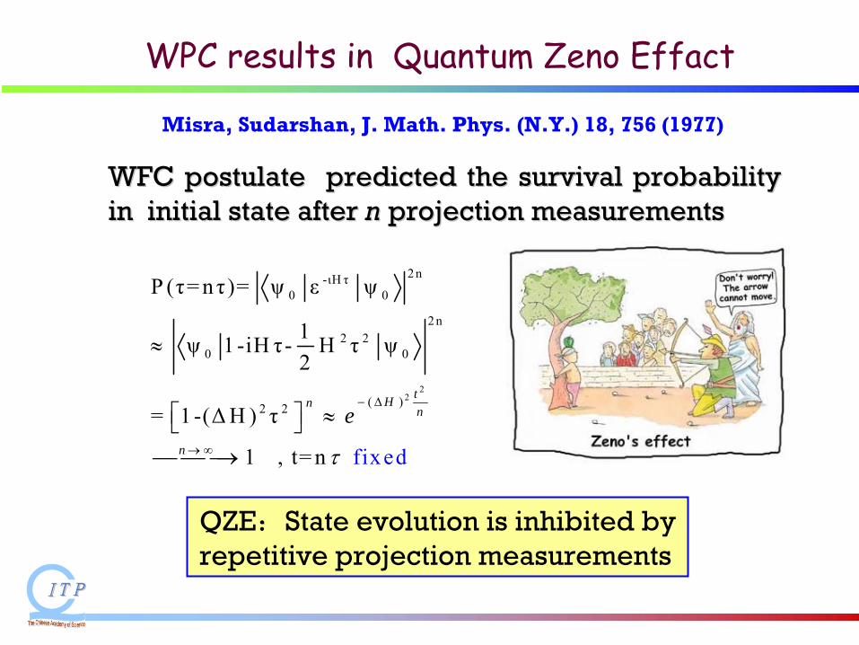
WPC results in Quantum Zeno Effact

22

2n-ιΗ τ0 0

2n2 2

0 0

( )2 2

P (τ= n τ )= ψ ε ψ

1ψ 1-iΗ τ - Η τ ψ2

= 1-(ΔΗ ) τ

1 , t= fixedn

tHnn

n

e

τ

− Δ

→ ∞

≈

⎡ ⎤ ≈⎣ ⎦⎯ ⎯ ⎯→

WFC postulate predicted the survival probability WFC postulate predicted the survival probability in in initial state after initial state after nn

projectioprojectionn

measurements measurements

Misra, Sudarshan, J. Math. Phys. (N.Y.) 18, 756 (1977)

QZE：State evolution is inhibited by repetitive projection measurements

Experiments Testing QZE

Seem to well support von Neumann's projection postulate !

Trapped Ion:

Wineland’group,

Phys. Rev. A 41, 2295 (1990) Cold atoms:

Raizen’s Group, Phys. Rev. Lett. 87, 040402 (2001)

BEC:

Pritchard’

group, Phys. Rev. Lett. 97, 260402 (2006) Cavity QED:

Haroche’s group, Phys. Rev. Lett.

101, 180402 (2008)

Is the von Neumann‘s projection postulate necessary for explaining these existing experiments

of QZE

?

Recall: C. P. Sun, in Quantum Classical Correspondence: The 4th Drexel Symposium on Quantum Nonintegrability, 1994, edited by D. H. Feng and B. L. Hu (International Press, Cambridge, MA), p. 99.For a review, see C. P. Sun, X. X. Yi and X. J. Liu, Fortschr. Phys. 43, 585 (1995).

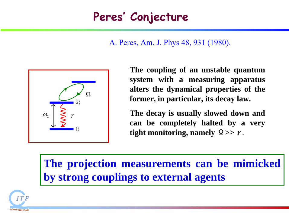
Peres’

Conjecture

The coupling of an unstable quantum system with a measuring apparatus alters the dynamical properties of the former, in particular, its decay law.

The decay is usually slowed down and can be completely halted by a very tight monitoring, namely Ω>>γ.

A. Peres, Am. J. Phys 48, 931 (1980).

1

2

2ω γ

Ω

The projection measurements can be mimicked by strong couplings to external agents

Foundamental Problems in QM

Can the results from projection measurements be generally realized

by special couplings to

external agents –

measuring apparatus？

QZE (or QAZE) depends on quantum mechanics interpretation (QMI), or is Universal ?

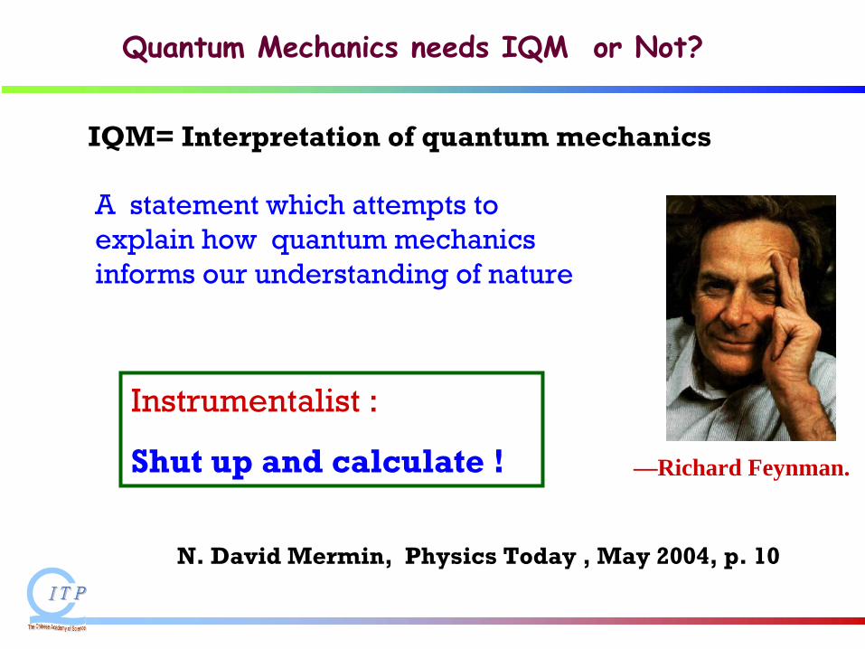
N. David Mermin, Physics Today , May 2004, p. 10

Instrumentalist :

Shut up and calculate !

IQM= Interpretation of quantum mechanics

A statement which attempts to explain how quantum mechanics informs our understanding of nature

—Richard Feynman.

Quantum Mechanics needs IQM or Not?

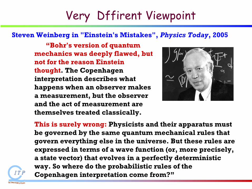
“Bohr's version of quantum mechanics was deeply flawed, but not for the reason Einstein thought. The Copenhagen interpretation describes what happens when an observer makes a measurement, but the observer and the act of measurement are themselves treated classically.

Steven Weinberg in "Einstein's Mistakes", Physics Today,

2005

This is surely wrong: Physicists and their apparatus must be governed by the same quantum mechanical rules that govern everything else in the universe. But these rules are expressed in terms of a wave function (or, more precisely, a state vector) that evolves in a perfectly deterministic way. So where do the probabilistic rules of the Copenhagen interpretation come from?”

Very Dffirent Viewpoint

Considerable progress has been made in recent years toward the resolution of the problem,…... It is enough to say that neither Bohr nor Einstein had focused on the real problem with quantum mechanics. The Copenhagen rules clearly work, so they have to be accepted. But this leaves the task of explaining them by applying the deterministic equation for the evolution of the wave function,

the Schrödinger equation, to

observers and their apparatus.

Steven Weinberg in "Einstein's Mistakes"

The problem of thinking in terms of classical measurements of a quantum system becomes particularly acute in the field of quantum cosmology, where the quantum system is the universe

1. Quantum Zeno effect (QZE)

"proves" projection measurement？

2 . No Projection in reality for QZE: Revisiting existing experiments

3. Reamrks on Foundamental problems:Two von Neumanns , two Physicses !

4. Anti-QZE for open quantum system in dynamics

Content

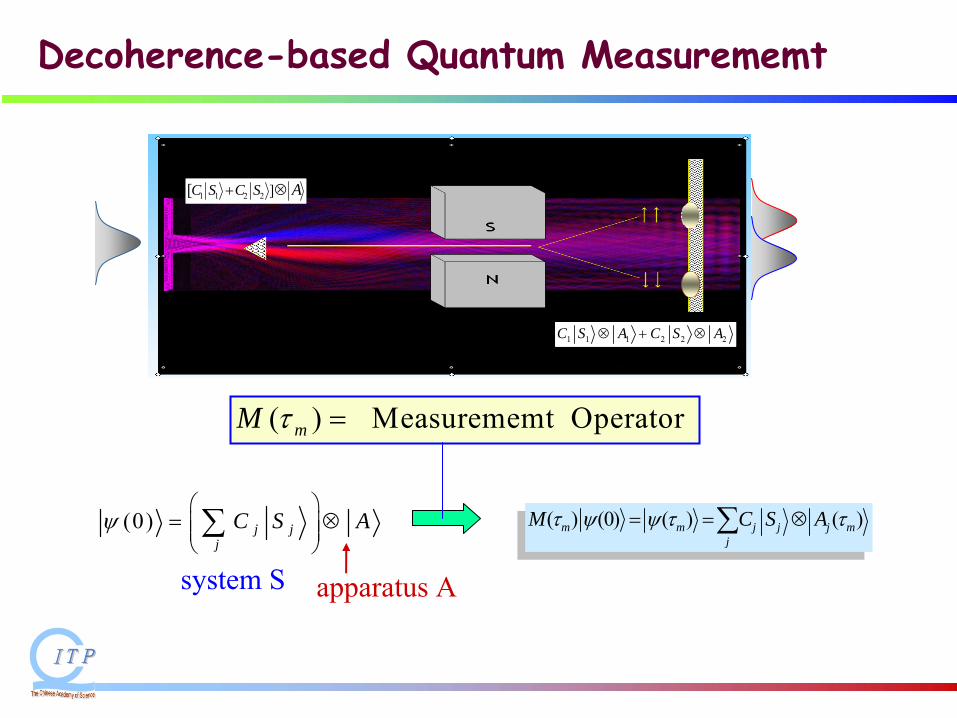
1 1 2 2 ][C S C S A+ ⊗

1 1 1 2 2 2C S A C S A⊗ + ⊗

Decoherence-based Quantum Measurememt

(0) j jj

C S Aψ⎛ ⎞⎜ ⎟⎜ ⎟⎝ ⎠

= ⊗∑

system

S apparatus

A

( ) (0) ( ) ( )m m j j j mj

M C S Aτ ψ ψ τ τ= = ⊗∑

( ) Measurememt Operator mM τ =

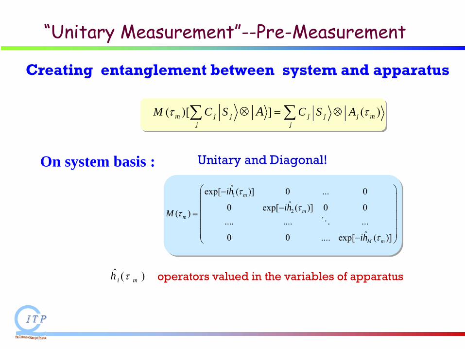
“Unitary Measurement”--Pre-Measurement

( )[ ] ( )m j j j j j mj j

M C S C S AAτ τ= ⊗⊗∑ ∑

Creating entanglement between system and apparatus

On system basis :

1

2

ˆexp[ ( )] 0 ... 0ˆ0 exp[ ( )] 0 0( )

.... .... ...ˆ0 0 .... exp[ ( )]

m

mm

M m

ih

ihM

ih

τ

ττ

τ

⎛ ⎞−⎜ ⎟⎜ ⎟−

= ⎜ ⎟⎜ ⎟⎜ ⎟−⎝ ⎠

operators

valued in the variables of

apparatusˆ ( )i mh τ

Unitary and Diagonal!

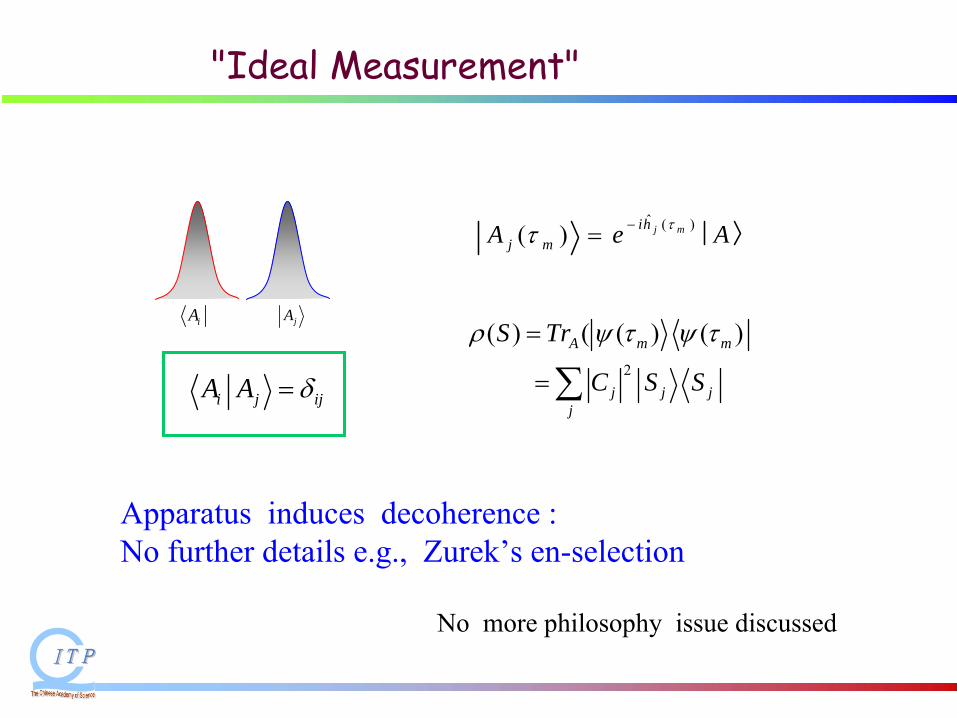
"Ideal Measurement"

ˆ ( )( ) j mihj mA e Aττ −=

i j ijA A δ=2

( ) ( ( ) ( )

A m m

j j jj

S Tr

C S S

ρ ψ τ ψ τ=

=∑

Apparatus induces decoherence : No further details e.g., Zurek’s en-selection

No more philosophy issue discussed

jAiA

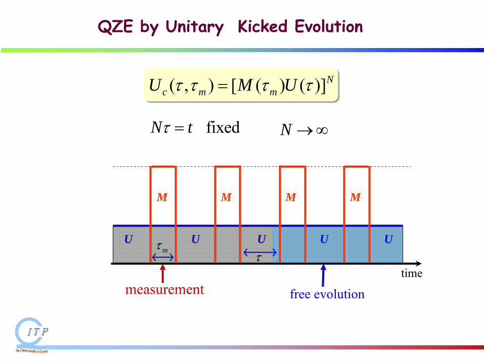
QZE by Unitary Kicked Evolution

timeτ

U U U U U

M M M M

measurement

( , ) [ ( ) ( )]Nc m mU M Uτ τ τ τ=

mτ

free evolution

fixedN tτ = N →∞

Nm

tiHmc

Nm MeUUM d )(),()]()([lim

0τττττ

τ

−

→≡→

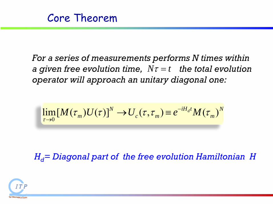
Hd

= Diagonal part of the free evolution Hamiltonian H

For a series of measurements performs N times within a given free evolution time, the total evolution operator will approach an unitary diagonal one:

Core Theorem

N tτ =

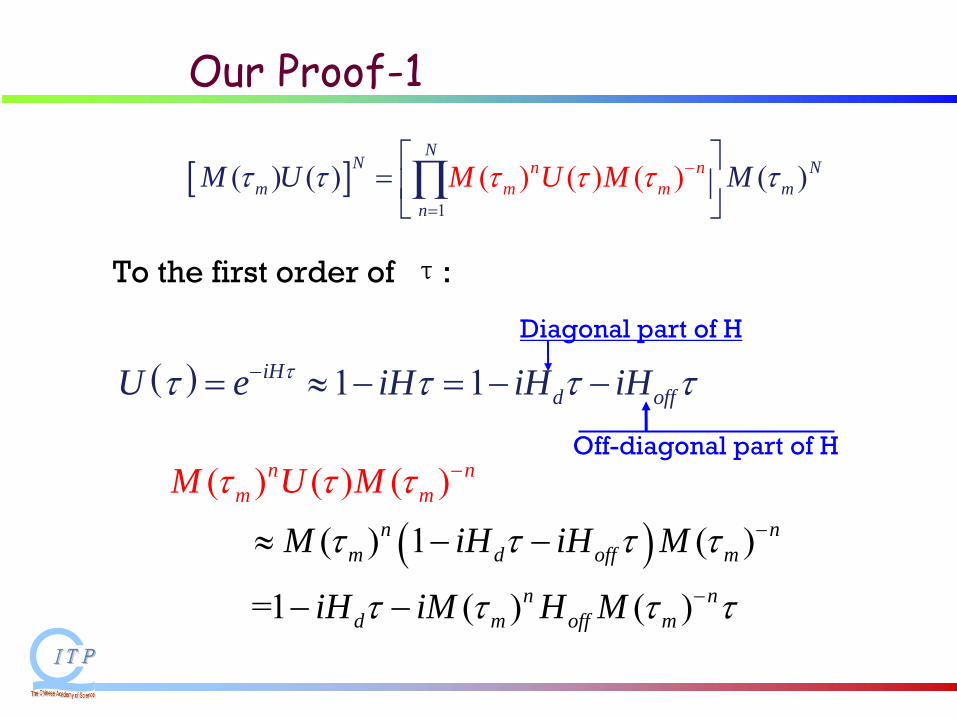
Our Proof-1

[ ]1

( ) ( ) )) ( ( ) (( )n nm

N

nm

NN

m mM U MMM Uτ τ ττ ττ=

−⎡ ⎤= ⎢ ⎥⎣ ⎦∏

( ) 1 1iHd offU e iH iH iHττ τ τ τ−= ≈ − = − −

Diagonal part of H

Off-diagonal part of H

( ) ( ) 1 ( )

=1

( ) ( ) ( )

( ) ( )

n nm d off m

n nd m off

n nm

m

m

M iH iH M

i i

M

H H M

U M

M

τ τ τ τ

τ τ τ τ

τ τ τ

−

−

−≈ − −

− −

To the first order of τ:

1

1

1 1

( ) ( )

= ( ) ( )

(

1

( ) ) ( ) 1N

dn

Nn n

Nn

m off mn

m mn n

Nn n

m offd mn

M U M H M

it M

i H

i

i

MN

H Ht

M ττ

τ

τ τ

τ

τ ττ −

=

−

=

−

=

=

−= −

−−

∑ ∑∏

∑

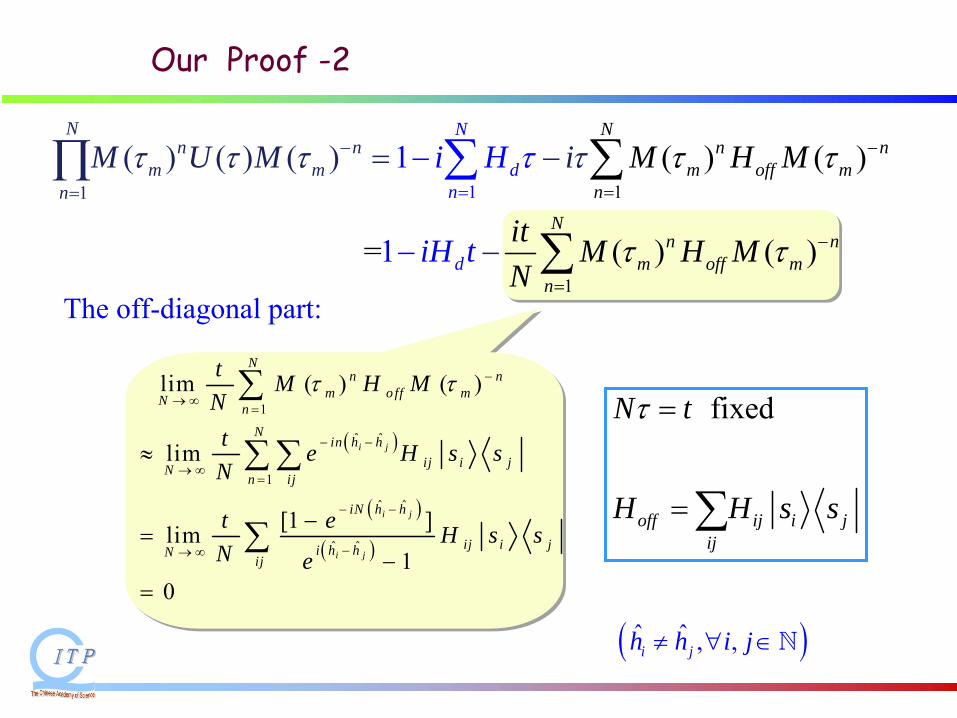
Our Proof -2

fixed

off ij i jij

N t

H H s s

τ =

=∑

( )

( )

( )

1

ˆ ˆ

1

ˆ ˆ

ˆ ˆ

lim ( ) ( )

lim

[1 ]lim1

0

i j

i j

i j

Nn n

m off mN n

Nin h h

ij i jNn ij

iN h h

ij i ji h hNij

t M H MNt e H s sN

t e H s sN e

τ τ −

→ ∞=

− −

→ ∞=

− −

−→ ∞

≈

−=

−=

∑

∑∑

∑

The off-diagonal part:

( )ˆ ˆ , ,i jh h i j≠ ∀ ∈N

1 11

( ) ( )( ) ( ) ( ) 1N

n nN

n nm m o

N

dm ffnnn

mi t MiHN

M M H MU τ τ ττ τ τ=

−

==

−= −− ∑∏ ∑

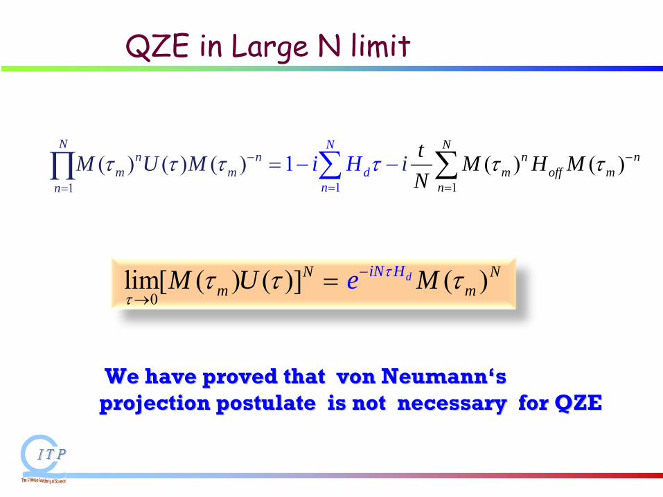
QZE in Large N limit

0lim[ ( ) ( )] ( )diN N

m mN HeM U Mτ

ττ τ τ−

→=

We have proved that We have proved that von Neumannvon Neumann‘‘s s projection postulate projection postulate is not is not necessary fornecessary for

QZEQZE

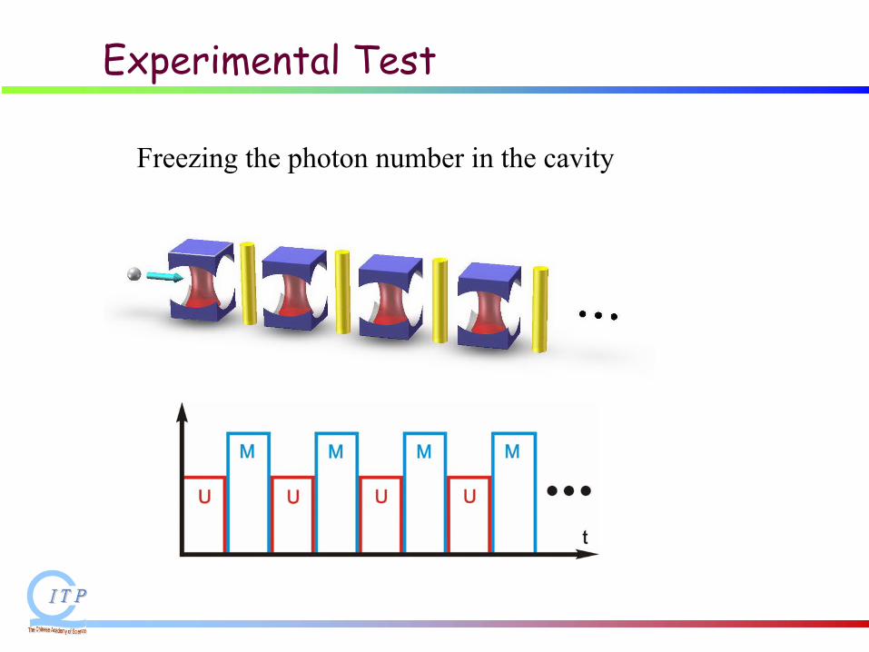
Experimental Test

Freezing the photon number in the cavity

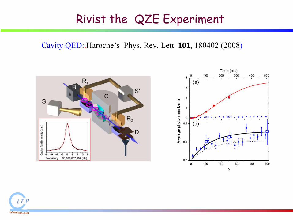
Rivist the QZE Experiment

Cavity QED:.Haroche’s Phys. Rev. Lett. 101, 180402 (2008)

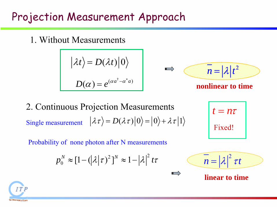
Projection Measurement Approach

†( )( ) a aD e α αα∗−=

( ) 0t D tλ λ=2n tλ=

( ) 0 0 1Dλτ λτ λτ= = +

220 [1 ( ) ] 1N Np tλ τ λ τ≈ − ≈ − 2n tλ τ=

t nτ=

1. Without Measurements

2. Continuous Projection Measurements

Single measurement

Probability of none photon after N measurements

Fixed!

2n tλ= 2n tλ= 2n tλ= 2n tλ= 2n tλ=

linear to time

nonlinear to time

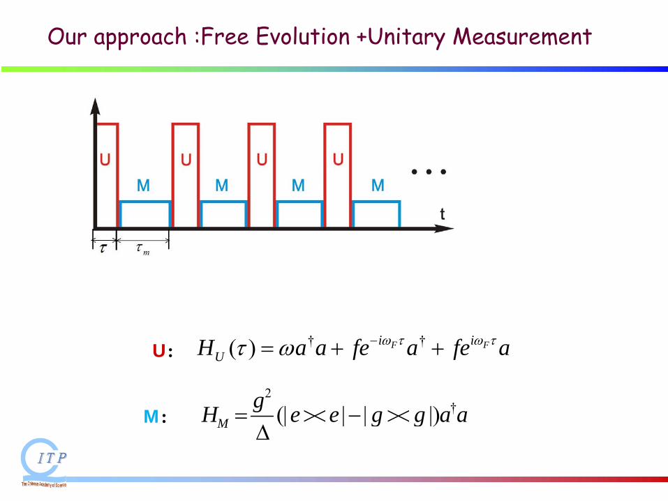
U:

M:

† †( ) F Fi iUH a a fe a fe aτω ω ττ ω −= + +

2†(| | | |)M

gH e e g g a a= >< − ><Δ

Our approach :Free Evolution +Unitary Measurement

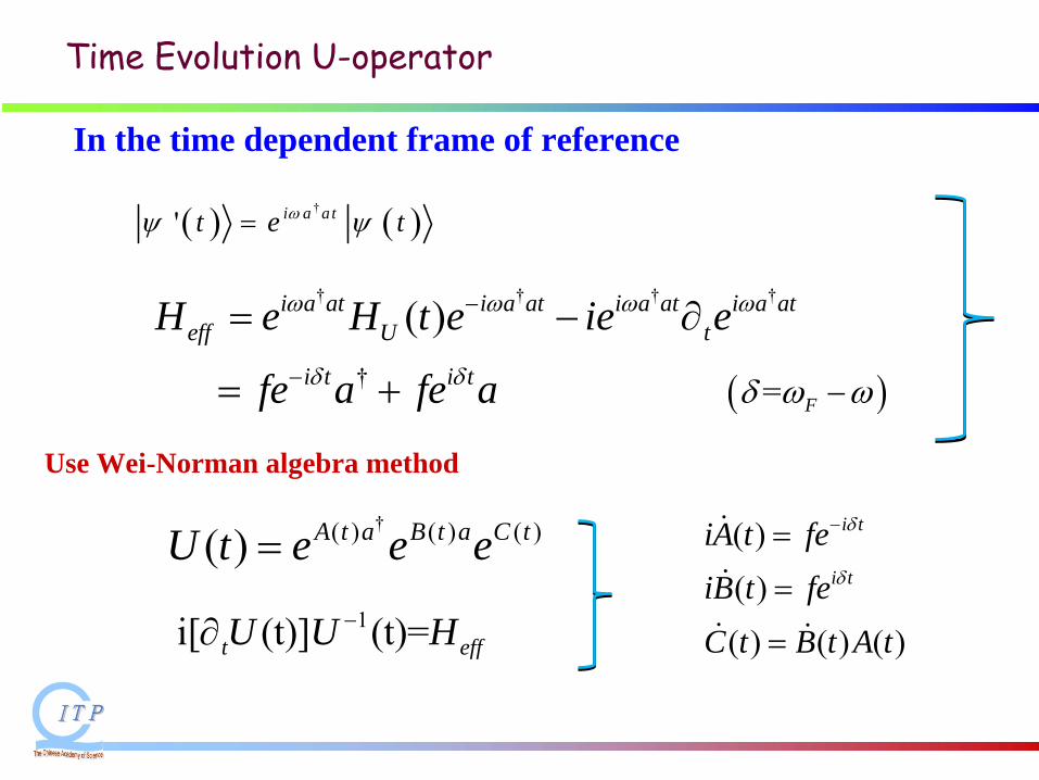
Time Evolution

U-operator

† † † †

†

( )i a at i a ateff

i a at i a atU t

i t i t

H

fe a f

e

e a

H t e ie eω ω ω

δ δ

ω

−

− − ∂=

= +

( ) ( )†

' i a a tet tωψ ψ=

In the time dependent frame of reference

( )= Fδ ω ω−

†( ) ( ) ( )( ) A t a B t a C tU t e e e=

1i[ (t)] (t)=t effU U H−∂

Use Wei-Norman algebra method

( )( )

( ) ( ) ( )

i t

i t

iA t feiB t fe

C t B t A t

δ

δ

−=

=

=

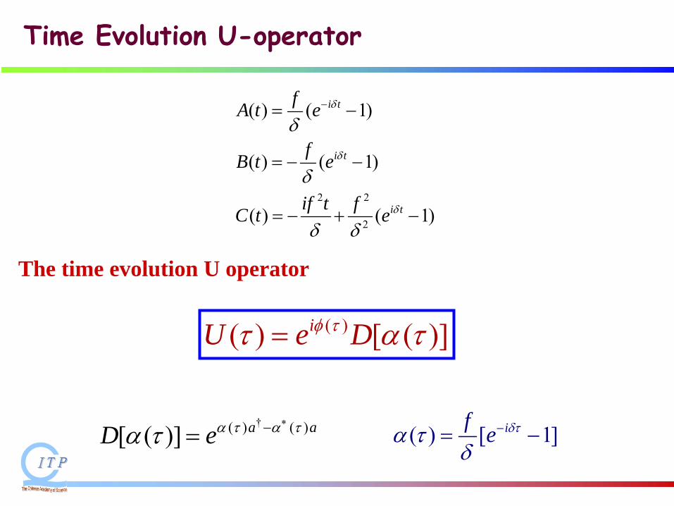
( )( ) [ ( )]iU e Dφ ττ α τ=

( ) [ 1]if e δτα τδ

−= −†( ) ( )[ ( )] a aeD α τ α τα τ

∗−=

The time evolution U operator

2 2

2

( ) ( 1)

( ) ( 1)

( ) ( 1)

i t

i t

i t

fA t e

fB t e

if t fC t e

δ

δ

δ

δ

δ

δ δ

−= −

= − −

= − + −

Time Evolution

U-operator

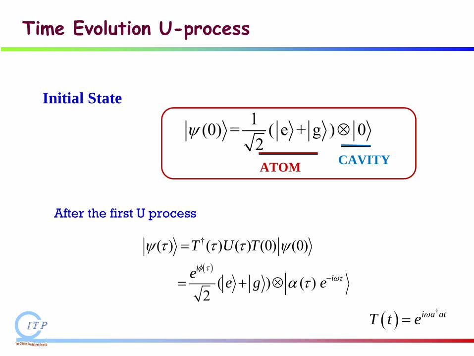
Initial State1(0) = ( e + g ) 02

ψ ⊗

ATOM CAVITY

( )

†( ) ( ) ( ) (0) (0)

( ) ( )2

ii

T U T

e e g eφ τ

ωτ

ψ τ τ τ ψ

α τ −

=

= + ⊗

After the first U process

Time Evolution

U-process

( ) †i a atT t e ω=

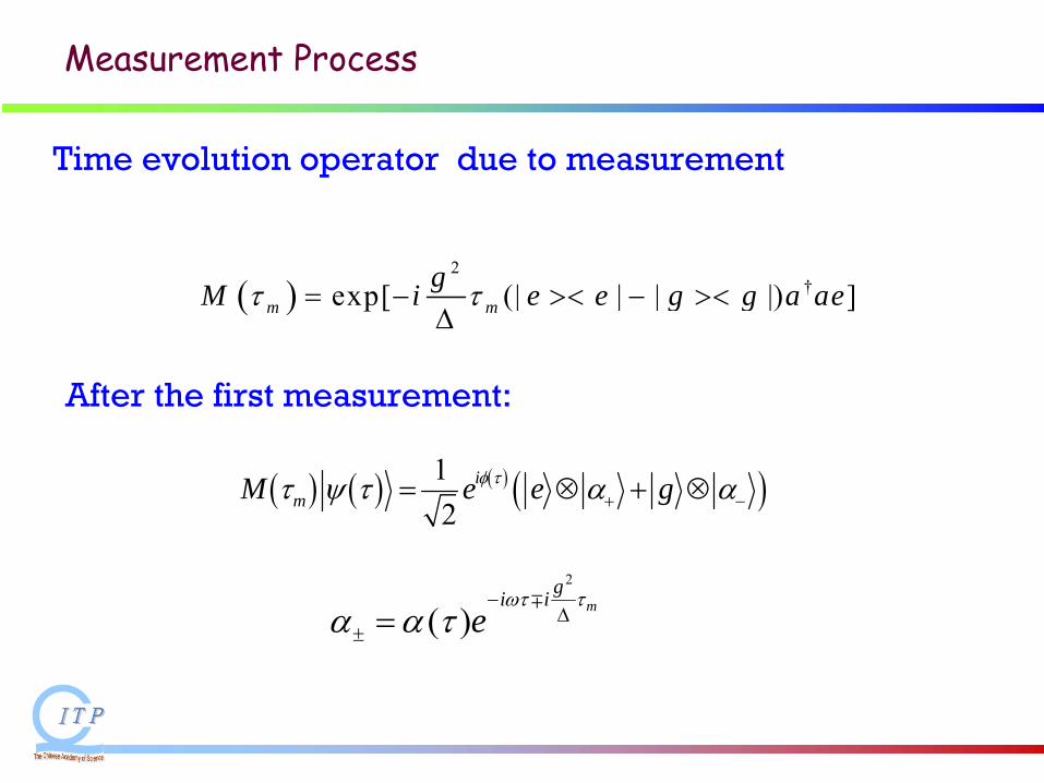
Measurement Process

( ) ( ) ( ) ( )12

imM e e gφ ττ ψ τ α α+ −= ⊗ + ⊗

Time evolution operator due to measurement

After the first measurement:

2

( ) mgi i

eωτ τ

τα α±

−Δ=

∓

( )2

†exp[ (| | | |) ]m mgM i e e g g a aeτ τ= − >< − ><Δ

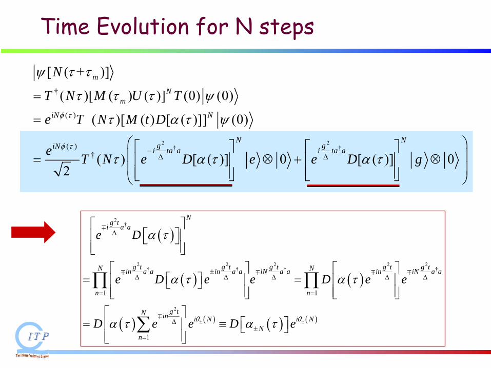
2 2† †

( ) �

(

†

)†

( )[ ( ) ( )] (0) (0)

( )[ ( ) [ ( )]] (0)

[ ( + )

( ) [ ( )] 0 [ ( ]

]

) 02

Nm

iN N

N Ng giN i ta a i

m

ta a

T N M U T

e T N M t D

e T N e D e e D g

N

φ τ

φ τ

τ τ τ ψ

τ α τ ψ

τ α τ α

τ τ

τ

ψ

−Δ Δ

=

⎛ ⎞⎡ ⎤ ⎡ ⎤⎜ ⎟= ⊗ + ⊗⎢ ⎥ ⎢ ⎥⎜ ⎟⎢ ⎥ ⎢ ⎥⎣ ⎦ ⎣⎝ ⎠

=

⎦

( )

( ) ( )

( ) ( ) ( ) ( )

2†

2 2 2 2 2† † † †

2

1 1

1

Ng ti a a

g t g t g t g t g tN Nin a a in a a iN a a in iN a a

n n

g tN in i N i NN

n

e D

e D e e D e e

D e e D eθ θ

α τ

α τ α τ

α τ α τ± ±

Δ

±Δ Δ Δ Δ Δ

= =

Δ±

=

⎡ ⎤⎡ ⎤⎢ ⎥⎣ ⎦

⎢ ⎥⎣ ⎦⎡ ⎤ ⎡ ⎤

= =⎡ ⎤⎢ ⎥ ⎢ ⎥⎣ ⎦⎢ ⎥ ⎢ ⎥⎣ ⎦ ⎣ ⎦⎡ ⎤

= ≡ ⎡ ⎤⎢ ⎥ ⎣ ⎦⎢ ⎥⎣ ⎦

∏ ∏

∑

∓

∓ ∓ ∓ ∓

∓

Time Evolution for N steps

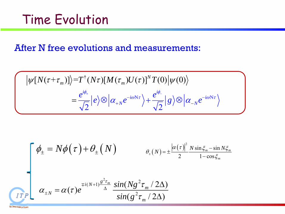
Time Evolution

†

N N

( )[ ( ) ( )] (0) (0[ ( + ) )

2

=

2

] N

i ii i

N N

mm

e ee

N T N

e g

M U T

eφ φ

ω τ ω τ

τ τψ τ τ

α α

τ ψ+ −

− −+ −⊗ + ⊗=

After N free evolutions and measurements:

2 2( 1)

2

( / 2 )( )( / 2 )

mgi N m

mN

sin Ngesin g

τ τττ

α α+

Δ±

Δ=

Δ

∓

( ) ( ) 2sin sin

2 1 cosm m

m

N NNα τ ξ ξθ

ξ±

−= ±

−( ) ( )N Nφ φ τ θ± ±= +

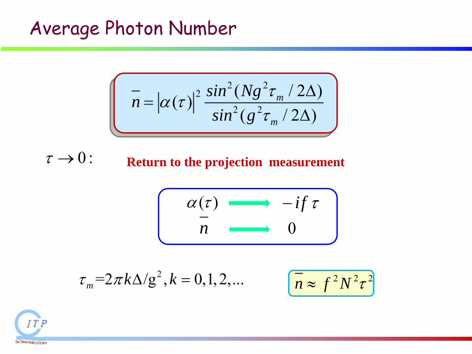
Average Photon Number

2 2 2n f N τ≈

0 :τ →

2 22

2 2

( / 2 )( )( / 2 )

m

m

sin Ngnsin g

τα ττ

Δ=

Δ

( )α τ if τ−n 0

2=2 /g , 0,1,2,...m k kτ π Δ =

Return to the projection measurement

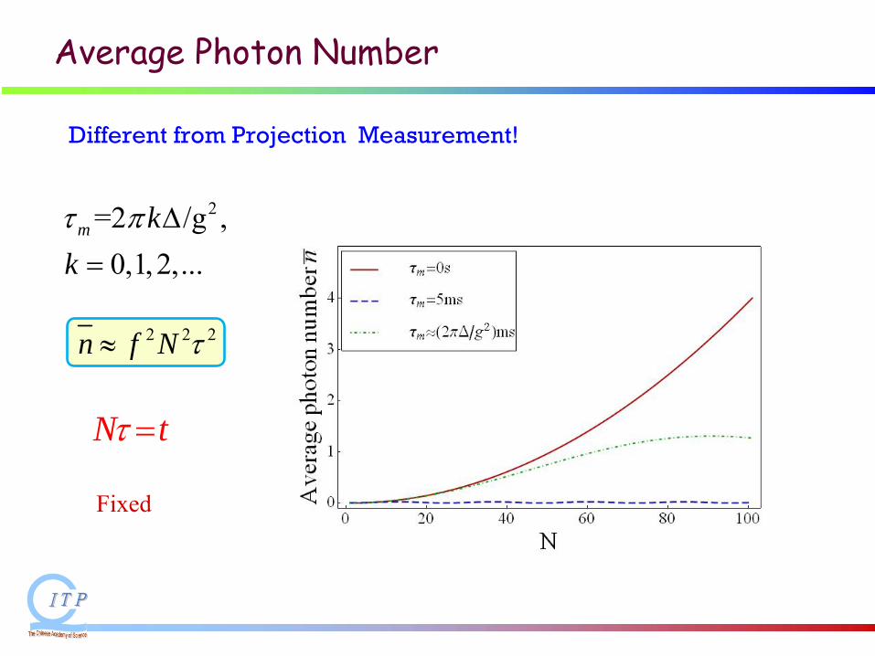
Average Photon Number

N tτ =

Fixed

Different from Projection

Measurement!

2=2 /g ,0,1,2,...

m kkτ π Δ=

2 2 2n f N τ≈

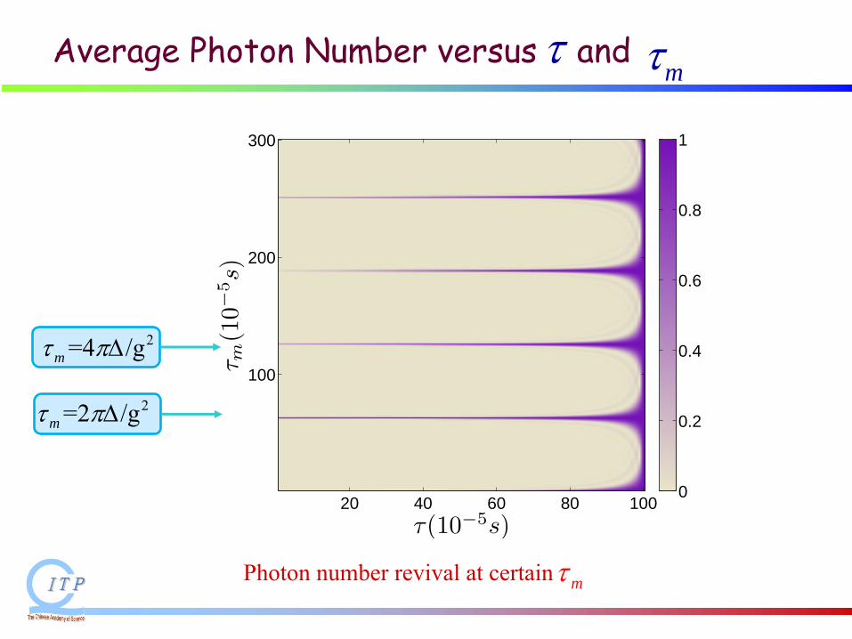
τ(10−5s)

τ m(1

0−5s)

20 40 60 80 100

100

200

300

0

0.2

0.4

0.6

0.8

1

Average Photon Number versus andτmτ

Photon number revival at certain mτ

2=2 /gmτ πΔ

2=4 /gmτ πΔ

1. Quantum Zeno effect (QZE)

"proves" projection measurement？

2 . No Projection in reality for QZE: Revisiting existing experiments

3. Reamrks on Foundamental problems:Two von Neumanns , two Physicses !

4. Anti-QZE for open quantum system in dynamics

Content

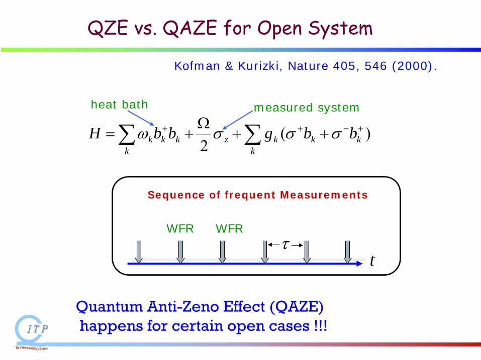
Kofman & Kurizki, Nature 405, 546 (2000).

QZE vs. QAZE for Open System

heat bath

WFRτ

t

Sequence of frequent Measurements

)(2

+−++ ++Ω

+= ∑∑ kkkk

zkkkk

bbgbbH σσσω

measured system

WFR

Quantum Anti-Zeno Effect (QAZE)happens for certain open cases !!!

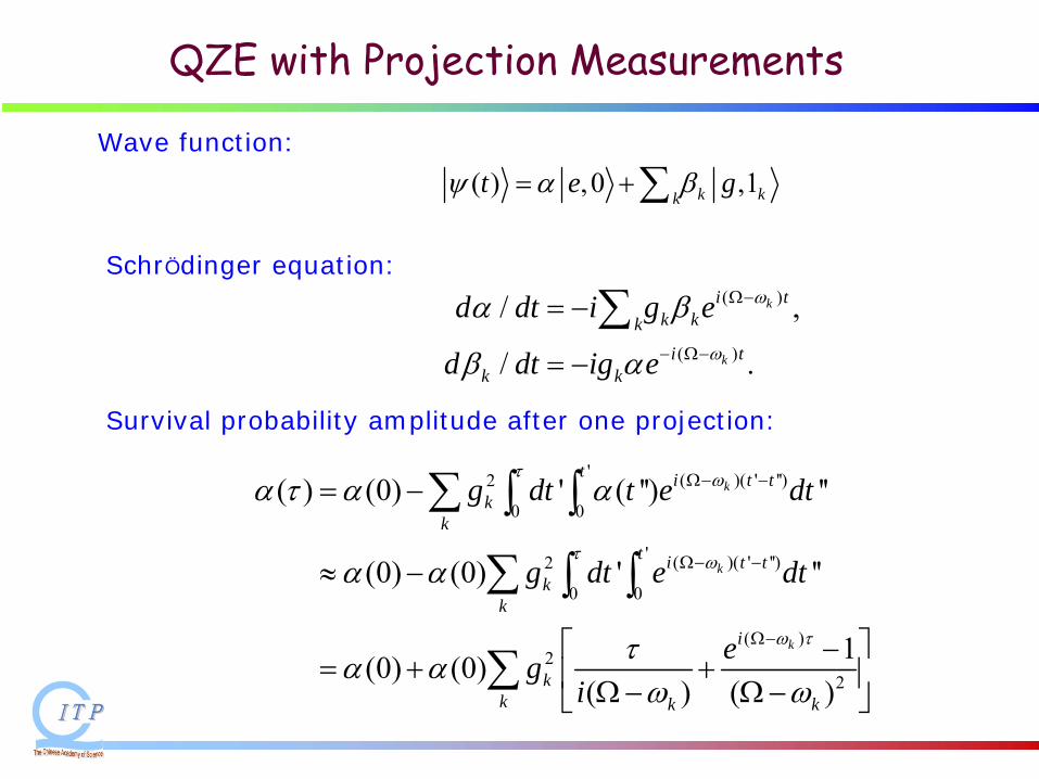
QZE with Projection Measurements

( ) ,0 ,1k kkt e gψ α β= +∑

Wave function:

( )

( )

/ ,

/ .

k

k

i tk kk

i tk k

d dt i g e

d dt ig e

ω

ω

α β

β α

Ω−

− Ω−

= −

= −

∑SchrÖdinger equation:

' ( )( ' '')2

0 0

' ( )( ' '')2

0 0

( )2

2

( ) (0) ' ( '') ''

(0) (0) ' ''

1(0) (0)( ) ( )

k

k

k

t i t tk

k

t i t tk

k

i

kk k k

g dt t e dt

g dt e dt

egi

τ ω

τ ω

ω τ

α τ α α

α α

τα αω ω

Ω− −

Ω− −

Ω−

= −

≈ −

⎡ ⎤−= + +⎢ ⎥Ω− Ω−⎣ ⎦

∑ ∫ ∫

∑ ∫ ∫

∑

Survival probability amplitude after one projection:

QZE with Projection Measurements

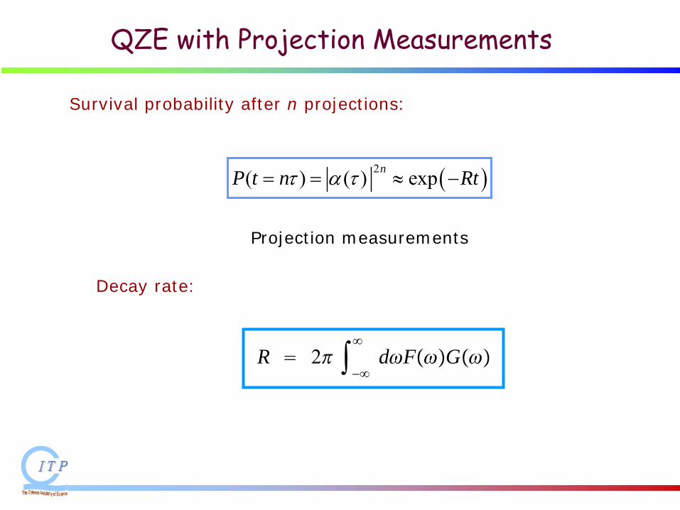
( )2( ) ( ) expnP t n Rtτ α τ= = ≈ −

Survival probability after n projections:

Projection measurements

R 2 −

dFG

Decay rate:

Nature 405, 546 (2000).

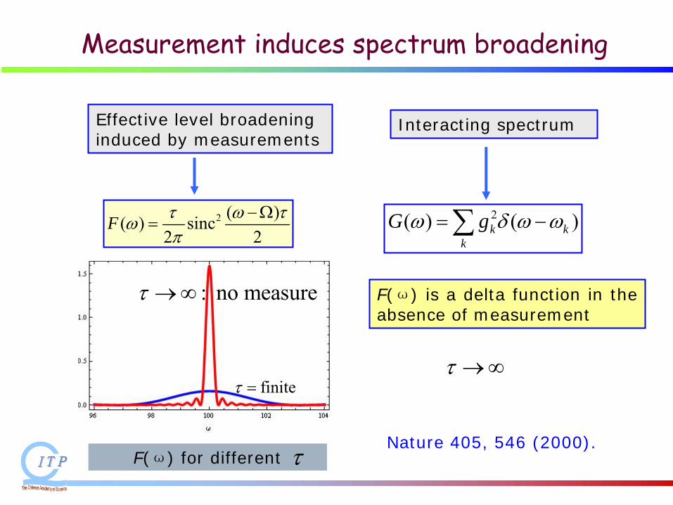
Measurement induces spectrum broadening

2 ( )( ) sinc2 2

F τ ω τωπ

−Ω= 2( ) ( )k k

kG gω δ ω ω= −∑

F(ω) is a delta function in the absence of measurement

F(ω) for different τ

: no measureτ →∞

finiteτ =τ →∞

Effective level broadening induced by measurements

Interacting spectrum

Zeno Effect

QZE by spectrums overlap

Anti-Zeno Effect !!!

Nature 405, 546 (2000).

R γ< R γ>

Question Anti-Zeno Effect

Kofman & Kurizki, (2000);

Fachi & Pascazio, (2001)

Decay of unstable state can be accelerated by measurements due to its couplings to reservoir

no QAZE if RWA is not made for some cases

Zheng et.al , PRL 101, 200404 (2008).

Ai, Li, Zheng, Sun, PRA 81, 042116 (2010).

QAZE happens without RWA is for some cases

For hydrogen spontaneous decay 2p-1s; 2p-1s

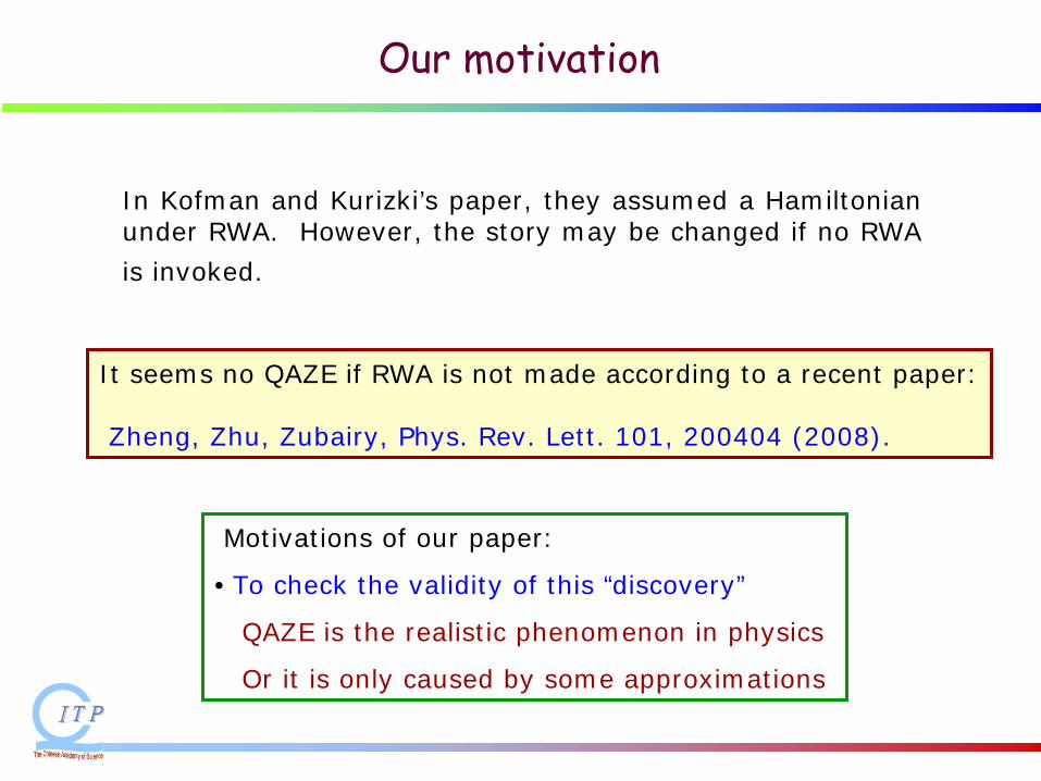
Our motivation

In Kofman and Kurizki’s paper, they assumed a Hamiltonian under RWA. However, the story may be changed if no RWA

is invoked.

Motivations of our paper:

• To check the validity of this “discovery”

QAZE is the realistic phenomenon in physics

Or it is only caused by some approximations

It seems no QAZE if RWA is not made according to a recent paper:

Zheng, Zhu, Zubairy, Phys. Rev. Lett. 101, 200404 (2008).

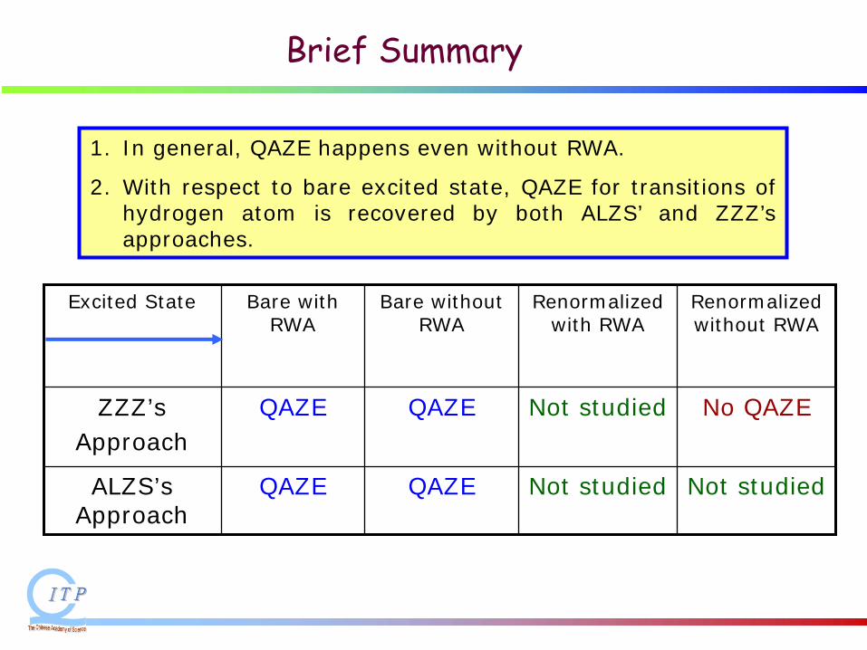
Brief Summary

Excited State Bare with RWA

Bare without RWA

Renormalized with RWA

Renormalized without RWA

ZZZ’sApproach

QAZE QAZE Not studied No QAZE

ALZS’s Approach

QAZE QAZE Not studied Not studied

1. In general, QAZE happens even without RWA.

2. With respect to bare excited state, QAZE for transitions of hydrogen atom is recovered by both ALZS’ and ZZZ’s approaches.

Our motivation

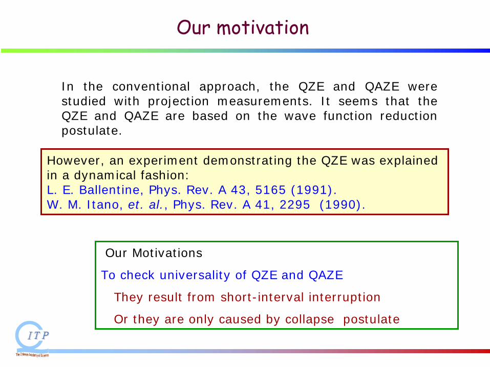
In the conventional approach, the QZE and QAZE were studied with projection measurements. It seems that the QZE and QAZE are based on the wave function reduction postulate.

Our Motivations

To check universality of QZE and QAZE

They result from short-interval interruption

Or they are only caused by collapse postulate

However, an experiment demonstrating the QZE was explained in a dynamical fashion:L. E. Ballentine, Phys. Rev. A 43, 5165 (1991).W. M. Itano, et. al., Phys. Rev. A 41, 2295 (1990).

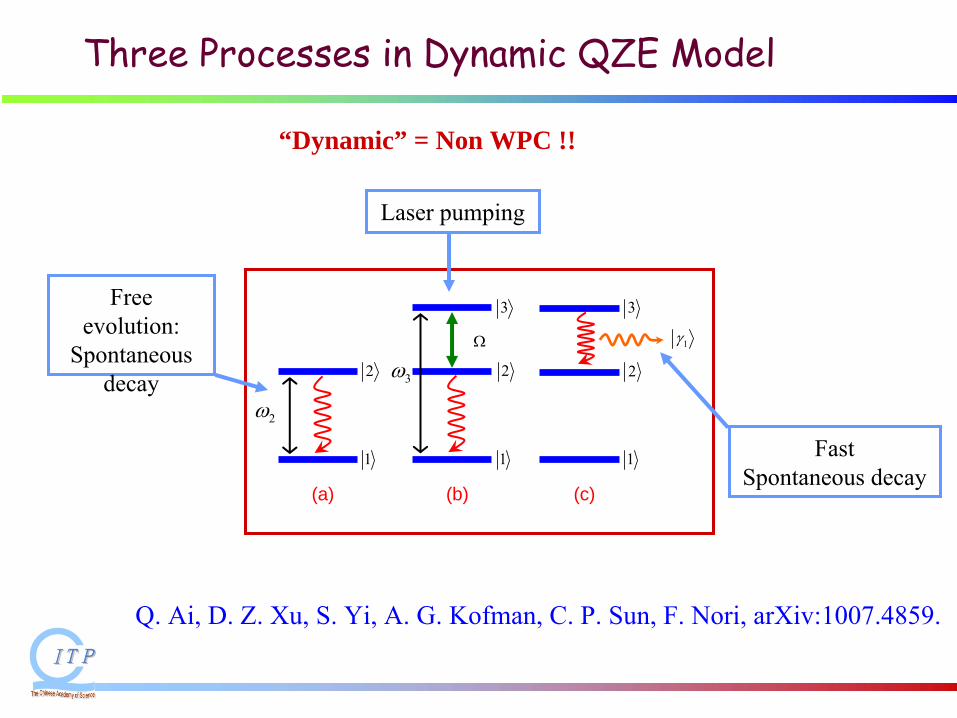
Three Processes in Dynamic QZE Model

(a)

1

2

2ω

(b)

1

2

3

Ω

3ω

(c)

1γ

1

2

3Free evolution:

Spontaneous decay

Laser pumping

Fast Spontaneous decay

Q. Ai, D. Z. Xu, S. Yi, A. G. Kofman, C. P. Sun, F. Nori, arXiv:1007.4859.

“Dynamic” = Non WPC !!

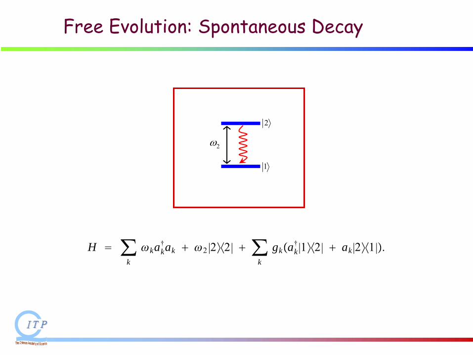
Free Evolution: Spontaneous Decay

1

2

2ω

H ∑k

kak†ak 2 |2⟨2| ∑

k

gkak† |1⟨2| ak |2⟨1|.

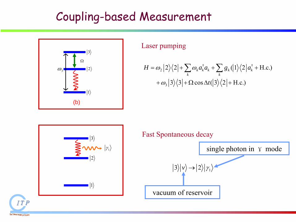
Coupling-based Measurement

(b)

1

2

3

Ω

3ω

Laser pumping

Fast Spontaneous decay

1γ

1

2

3

† †2

3

2 2 ( 1 2 H.c.)

3 3 cos ( 3 2 H.c.)

k k k k kk k

H a a g a

t

ω ω

ω

= + + +

+ +Ω Δ +

∑ ∑

13 2v γ→

vacuum of reservoir

single photon in γ mode

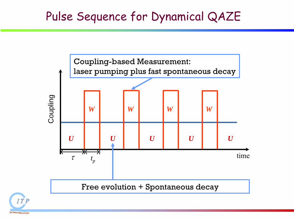
Pulse Sequence for Dynamical QAZE

timetpτ

U U U U U

W W W W

Cou

plin

g

Free evolution + Spontaneous decay

Coupling-based Measurement: laser pumping plus fast spontaneous decay

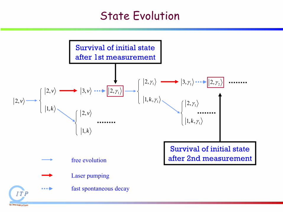
State Evolution

2,v

2,v

1,k2,v

1,k

3,v 12,γ12,γ

11, ,k γ12,γ

11, ,k γ

13,γ 22,γ

Survival of initial state after 1st measurement

Survival of initial state after 2nd measurementfree evolution

Laser pumping

fast spontaneous decay

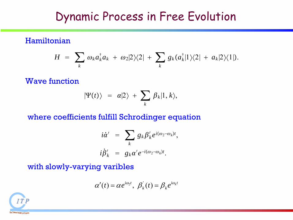
Dynamic Process in Free Evolution

Hamiltonian

Wave function

where coefficients fulfill Schrodinger equation

H ∑k

kak†ak 2|2⟨2| ∑

kgkak

† |1⟨2| ak |2⟨1|.

|t |2 ∑kk |1, k,

i′ ∑k

gkk′ ei2−kt,

ik′ gk′e−i2−kt.

with slowly-varying varibles

2( ) , ( ) ki ti tk kt e t e ωωα α β β′′ = =

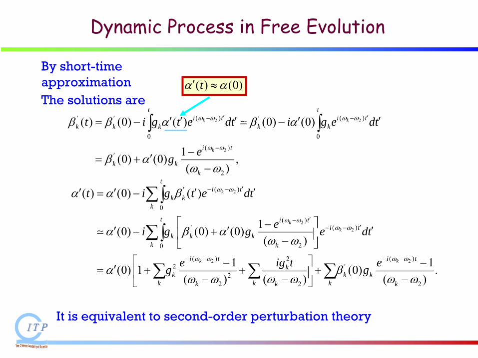
Dynamic Process in Free Evolution

By short-time approximationThe solutions are

It is equivalent to second-order perturbation theory

( ) (0)tα α′ ≈

2 2

2

( ) ( )

0 0( )

2

( ) (0) ( ) (0) (0)

1(0) (0) ,( )

k k

k

t ti t i t

k k k k k

i t

k kk

t i g t e dt i g e dt

eg

ω ω ω ω

ω ω

β β α β α

β αω ω

′ ′− −′ ′ ′

−′

′ ′ ′ ′ ′= − −

−′= +−

∫ ∫

2

22

2 2

( )

0

( )( )

20

( ) ( )22

22 2 2

( ) (0) ( )

1(0) (0) (0)( )

1 1(0) 1 (0) .( ) ( ) ( )

k

kk

k k

ti t

k kk

t i ti t

k k kk k

i t i tk

k k kk k kk k k

t i g t e dt

ei g g e dt

e ig t eg g

ω ω

ω ωω ω

ω ω ω ω

α α β

α β αω ω

α βω ω ω ω ω ω

′− −′

′−′− −′

− − − −′

′ ′ ′ ′= −

⎡ ⎤−′ ′ ′− +⎢ ⎥−⎣ ⎦⎡ ⎤− −′= + + +⎢ ⎥− − −⎣ ⎦

∑∫

∑∫

∑ ∑ ∑

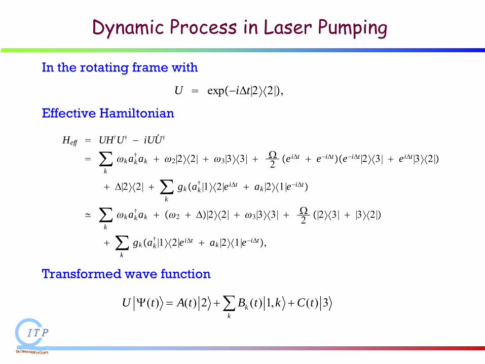
Dynamic Process in Laser Pumping

In the rotating frame with

Effective Hamiltonian

Transformed wave function

U exp−iΔt|2⟨2|,

( ) ( ) 2 ( ) 1, ( ) 3kk

U t A t B t k C tΨ = + +∑

Heff UH′U† − iUU†

∑kkak

†ak 2|2⟨2| 3|3⟨3| 2 eiΔt e−iΔte−iΔt |2⟨3| eiΔt |3⟨2|

Δ|2⟨2| ∑k

gkak† |1⟨2|eiΔt ak |2⟨1|e−iΔt

≃ ∑kkak

†ak 2 Δ|2⟨2| 3|3⟨3| 2 |2⟨3| |3⟨2|

∑k

gkak† |1⟨2|eiΔt ak |2⟨1|e−iΔt,

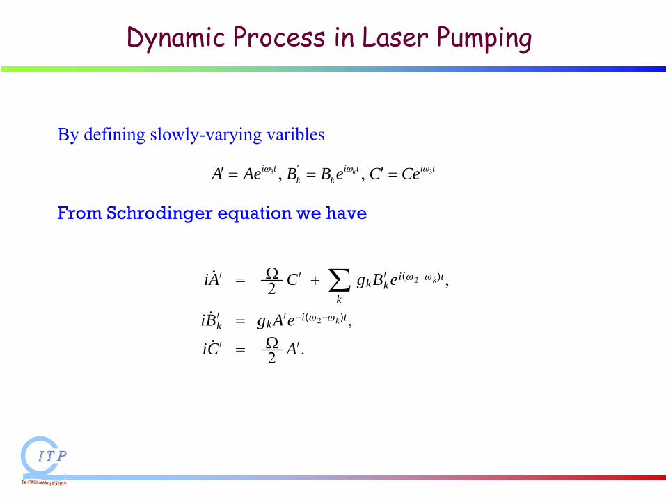
Dynamic Process in Laser Pumping

By defining slowly-varying varibles

3 3, , ki t i t i tk kA Ae B B e C Ceω ω ω′′ ′= = =

From Schrodinger equation we have

iA′ 2 C′ ∑

kgkBk

′ ei2−kt,

iBk′ gkA′e−i2−kt,

iC′ 2 A′.

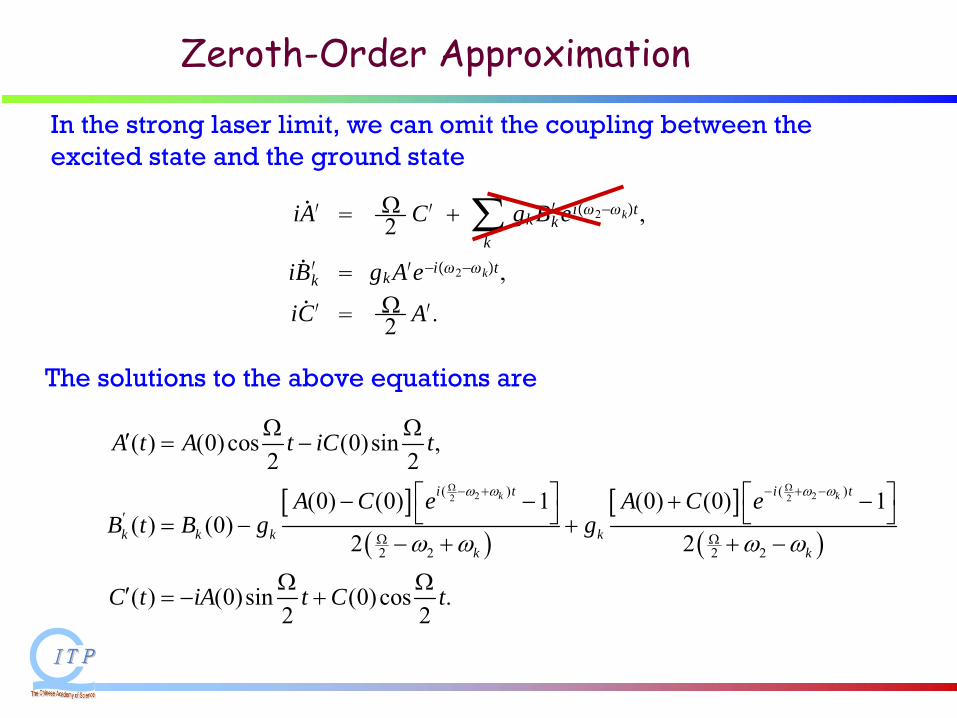
Zeroth-Order Approximation

[ ]( )

[ ]( )

2 22 2( ) ( )

2 22 2

( ) (0)cos (0)sin ,2 2

(0) (0) 1 (0) (0) 1( ) (0)

2 2

( ) (0)sin (0)cos .2 2

k ki t i t

k k k kk k

A t A t iC t

A C e A C eB t B g g

C t iA t C t

ω ω ω ω

ω ω ω ω

Ω Ω− + − + −

′

Ω Ω

Ω Ω′ = −

⎡ ⎤ ⎡ ⎤− − + −⎣ ⎦ ⎣ ⎦= − +− + + −

Ω Ω′ = − +

In the strong laser limit, we can omit the coupling between the excited state and the ground state

The solutions to the above equations are

iA′ 2 C′ ∑

kgkBk

′ ei2−kt,

iBk′ gkA′e−i2−kt,

iC′ 2 A′.

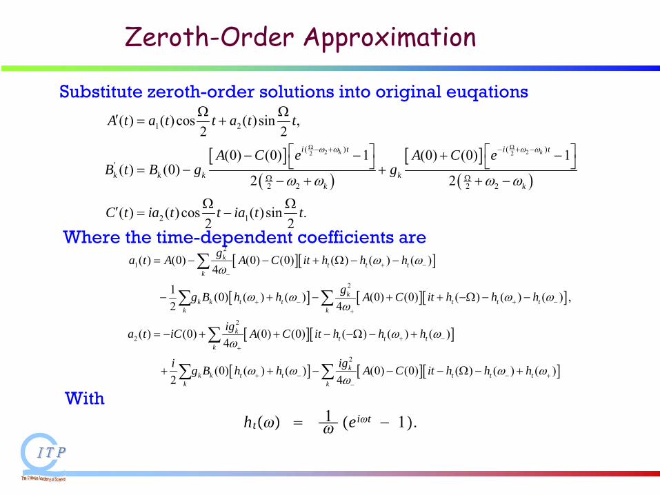
Zeroth-Order Approximation

Substitute zeroth-order solutions into original euqations

[ ]( )

[ ]( )

2 22 2

1 2

( ) ( )

2 22 2

2 1

( ) ( )cos ( )sin ,2 2

(0) (0) 1 (0) (0) 1( ) (0)

2 2

( ) ( )cos ( )sin .2 2

k ki t i t

k k k kk k

A t a t t a t t

A C e A C eB t B g g

C t ia t t ia t t

ω ω ω ω

ω ω ω ω

Ω Ω− + − + −

′

Ω Ω

Ω Ω′ = +

⎡ ⎤ ⎡ ⎤− − + −⎣ ⎦ ⎣ ⎦= − +− + + −

Ω Ω′ = −

Where the time-dependent coefficients are[ ][ ]

[ ] [ ][ ]

[ ][ ]

[ ]

2

1

2

2

2

( ) (0) (0) (0) ( ) ( ) ( )4

1 (0) ( ) ( ) (0) (0) ( ) ( ) ( ) ,2 4

( ) (0) (0) (0) ( ) ( ) ( )4

(0) ( ) ( )2

kt t t

k

kk k t t t t t

k k

kt t t

k

k k t tk k

ga t A A C it h h h

gg B h h A C it h h h

iga t iC A C it h h h

i ig B h h

ω ωω

ω ω ω ωω

ω ωω

ω ω

+ −−

+ − + −+

+ −+

+ −

= − − + Ω − −

− + − + + −Ω − −

= − + + − −Ω − +

+ + −

∑

∑ ∑

∑

∑ ∑ [ ][ ]2

(0) (0) ( ) ( ) ( )4

kt t t

g A C it h h hω ωω − +

−

− − Ω − +

ht 1 eit − 1.

With

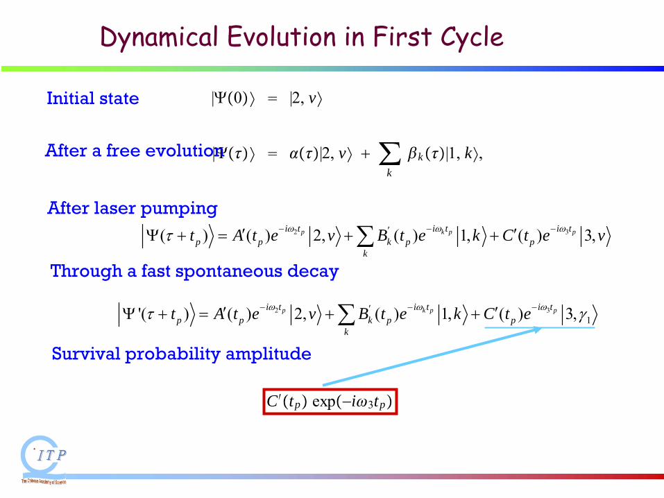
Dynamical Evolution in First Cycle

|0 |2, v

| |2, v ∑k

k|1, k,

C′tp exp−i3tp

Initial state

After a free evolution

After laser pumping

Through a fast spontaneous decay

Survival probability amplitude

.

2 3( ) ( ) 2, ( ) 1, ( ) 3,p k p pi t i t i tp p k p p

k

t A t e v B t e k C t e vω ω ωτ − − −′′ ′Ψ + = + +∑

2 31'( ) ( ) 2, ( ) 1, ( ) 3,p k p pi t i t i t

p p k p pk

t A t e v B t e k C t eω ω ωτ γ− − −′′ ′Ψ + = + +∑

|′2 2tp C′tpe−i3tp A′tpe−i2tp |2|1 ∑k

Bk′ tpe−iktp |1, k|1 C′tpe−i3tp |2|2

A1tpe−i2tp |2|v ∑k

Bk1tpe−iktp |1, k C1tpe−i3tp |2|1.

|2 2tp A′tpe−i2tp |2 ∑k

Bk′ tpe−iktp |1, k C′tpe−i3tp |3 C′tpe−i3tp |1

A1tpe−i2tp |2|v ∑k

Bk1tpe−iktp |1, k C1tpe−i3tp |3|v,

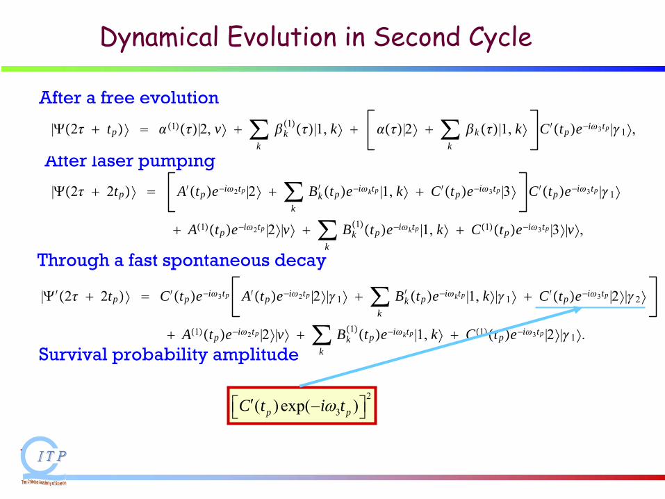
Dynamical Evolution in Second Cycle

2

3( )exp( )p pC t i tω′⎡ ⎤−⎣ ⎦

After a free evolution

After laser pumping

Through a fast spontaneous decay

Survival probability amplitude

.

|2 tp 1|2, v ∑kk1|1, k |2 ∑

kk|1, k C′tpe−i3tp |1,

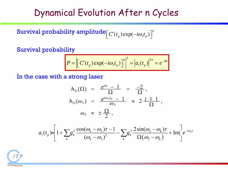
Dynamical Evolution After n Cycles

3( )exp( )n

p pC t i tω′⎡ ⎤−⎣ ⎦Survival probability amplitude

.

2 2

3 1( )exp( ) ( )n n Rt

p p pP C t i t a t eω −′⎡ ⎤= − = =⎣ ⎦

Survival probability

htp ei − 1

−2

,

htp eitp − 1

≈ 2 i ∓ 1

,

≈ 2 ,

In the case with a strong laser

( )22 22 2

1 22 2

cos( ) 1 2sin( )( ) 1 Im( )

ik kp k k

k kk k

a t g g e ω τω ω τ ω ω τω ω ω ω

−⎡ ⎤− − −≈ + − +⎢ ⎥− Ω −⎣ ⎦

∑ ∑

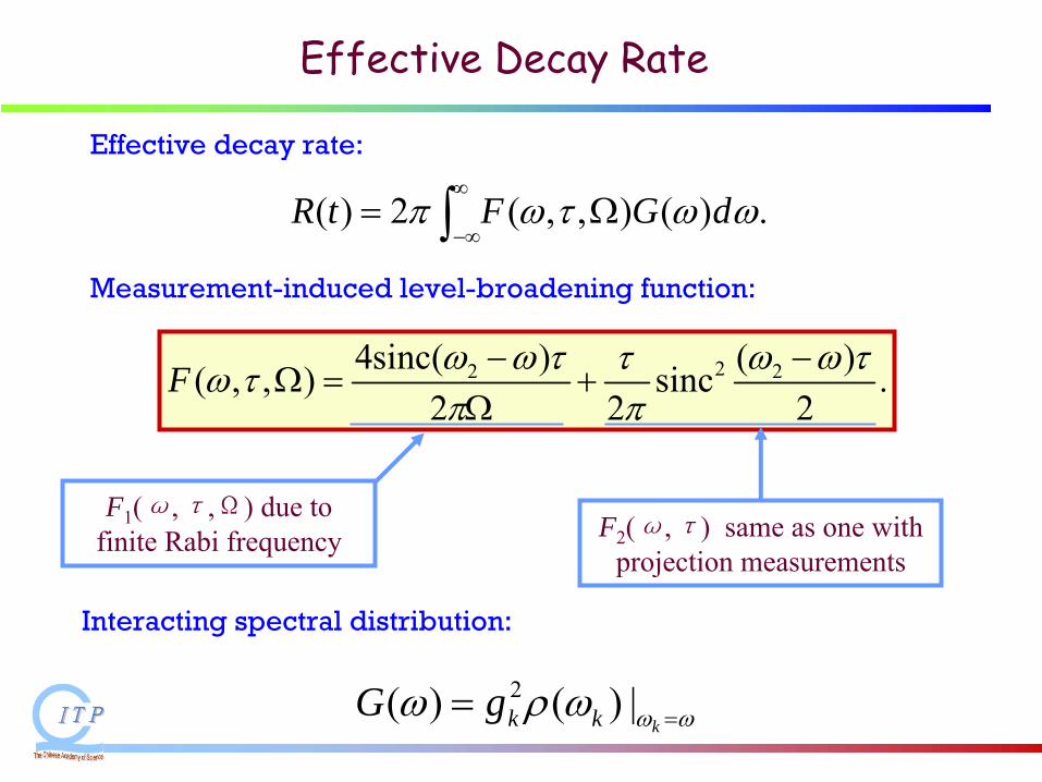
Effective Decay Rate

( ) 2 ( , , ) ( ) .R t F G dπ ω τ ω ω∞

−∞= Ω∫

22 24sinc( ) ( )( , , ) sinc .2 2 2

F ω ω τ ω ω ττω τπ π

− −Ω = +

Ω

Effective decay rate:

Measurement-induced level-broadening function:

F1

(ω,τ,Ω) due to finite Rabi frequency F2

(ω,τ) same as one with projection measurements

Interacting spectral distribution:

2( ) ( ) |kk kG g ω ωω ρ ω ==

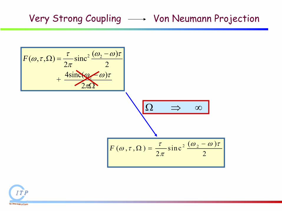
Very Strong Coupling

2 2

2

( )( , , ) sinc2 24sinc( ) +

2

F ω ω ττω τπ

ω ω τπ

−Ω =

−Ω

Von Neumann Projection

2 2( )( , , ) s inc2 2

F ω ω ττω τπ

−Ω =

Ω ⇒ ∞

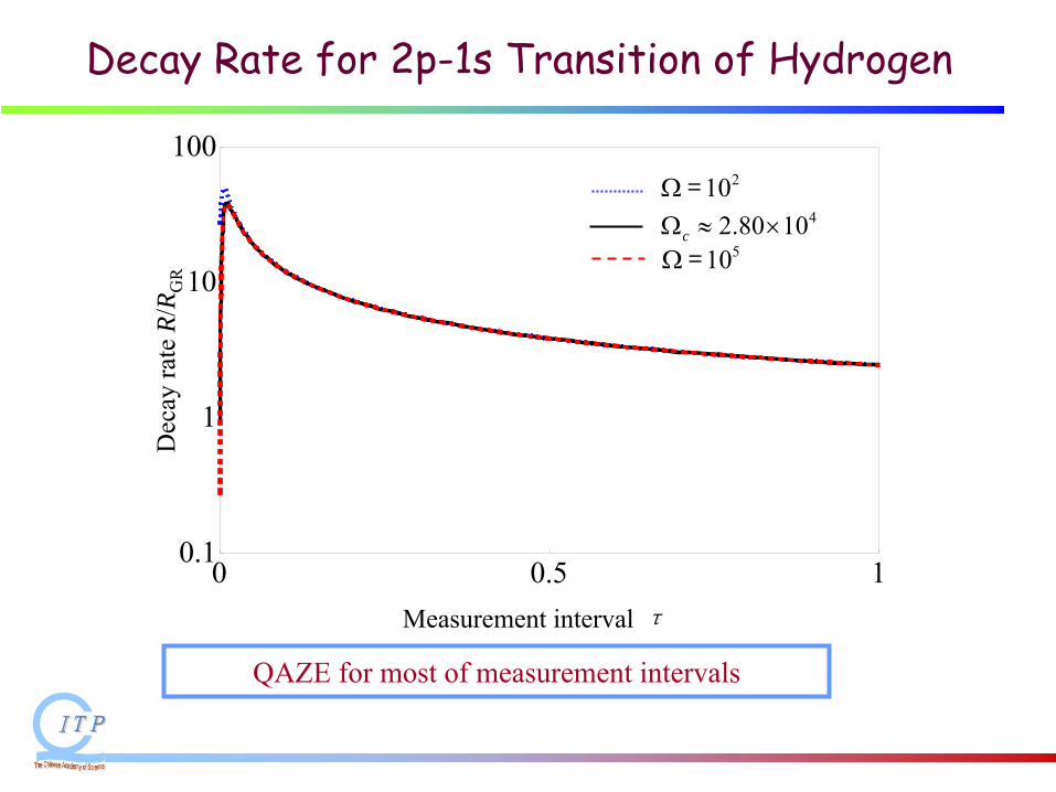
Decay Rate for 2p-1s Transition of Hydrogen

0 0.5 10.1

1

10

100210Ω =

42.80 10cΩ ≈ ×510Ω =

Dec

ay ra

te R

/RG

R

QAZE for most of measurement intervals

Measurement interval

τ

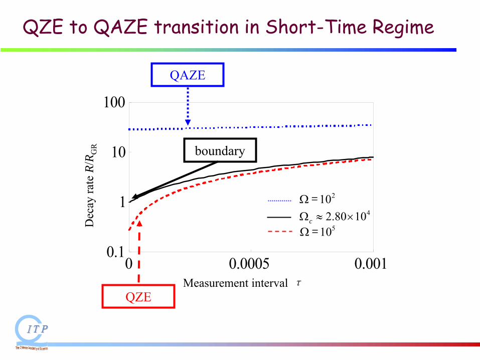
0 0.0005 0.0010.1

1

10

100

QZE to QAZE transition in Short-Time Regime

210Ω =42.80 10cΩ ≈ ×

510Ω =

Measurement interval

τ

Dec

ay ra

te R

/RG

R

QZE

QAZE

boundary

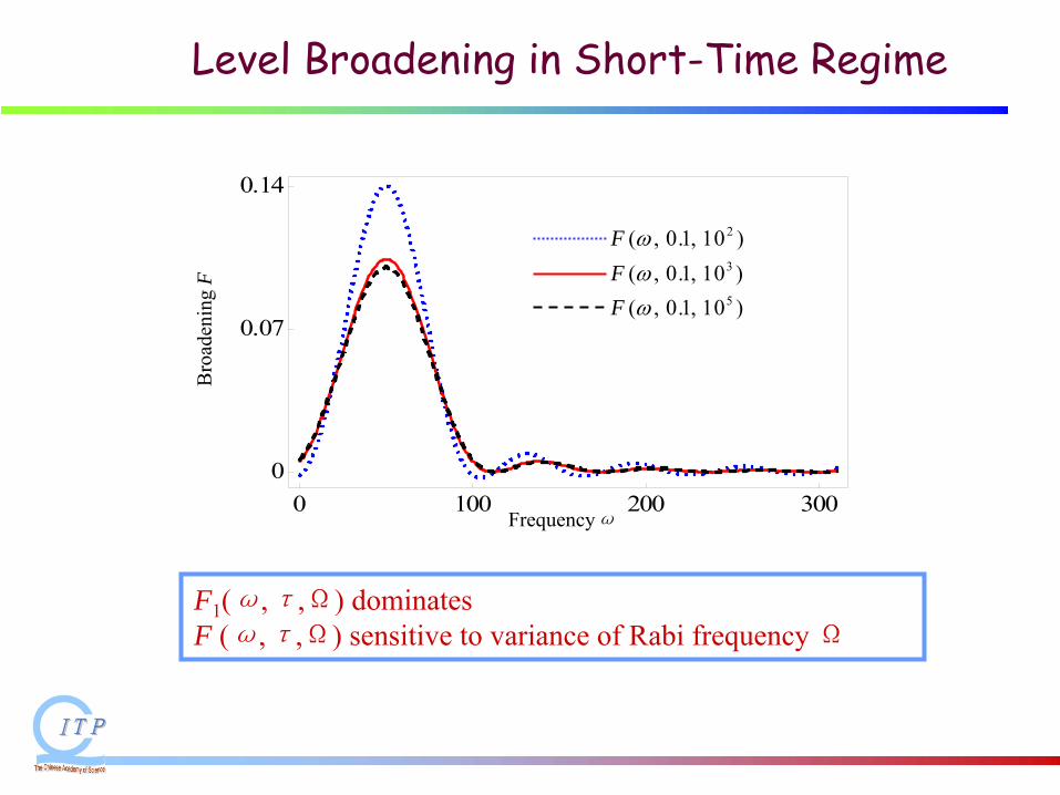
Level Broadening in Short-Time Regime

0 100 200 3000

0.07

0.14

2( , 0.1, 10 )F ω3( , 0.1, 10 )F ω5( , 0.1, 10 )F ω

Bro

aden

ing

F

Frequencyω

F1

(ω,τ,Ω) dominatesF (ω,τ,Ω) sensitive to variance of Rabi frequency Ω

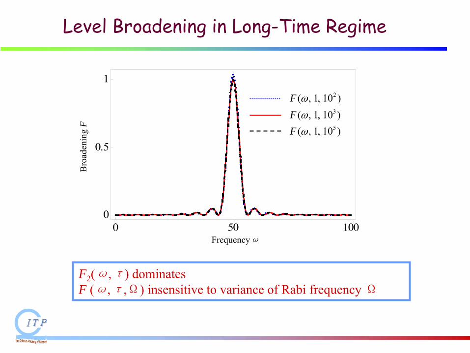
Level Broadening in Long-Time Regime

0 50 1000

0.5

12( , 1, 10 )F ω3( , 1, 10 )F ω5( , 1, 10 )F ω

Bro

aden

ing

F

Frequencyω

F2

(ω,τ) dominates F (ω,τ,Ω) insensitive to variance of Rabi frequency Ω