Embed Size (px)
Citation preview
1
Curves & Surfaces in CG
2
Position wrt previous lectures
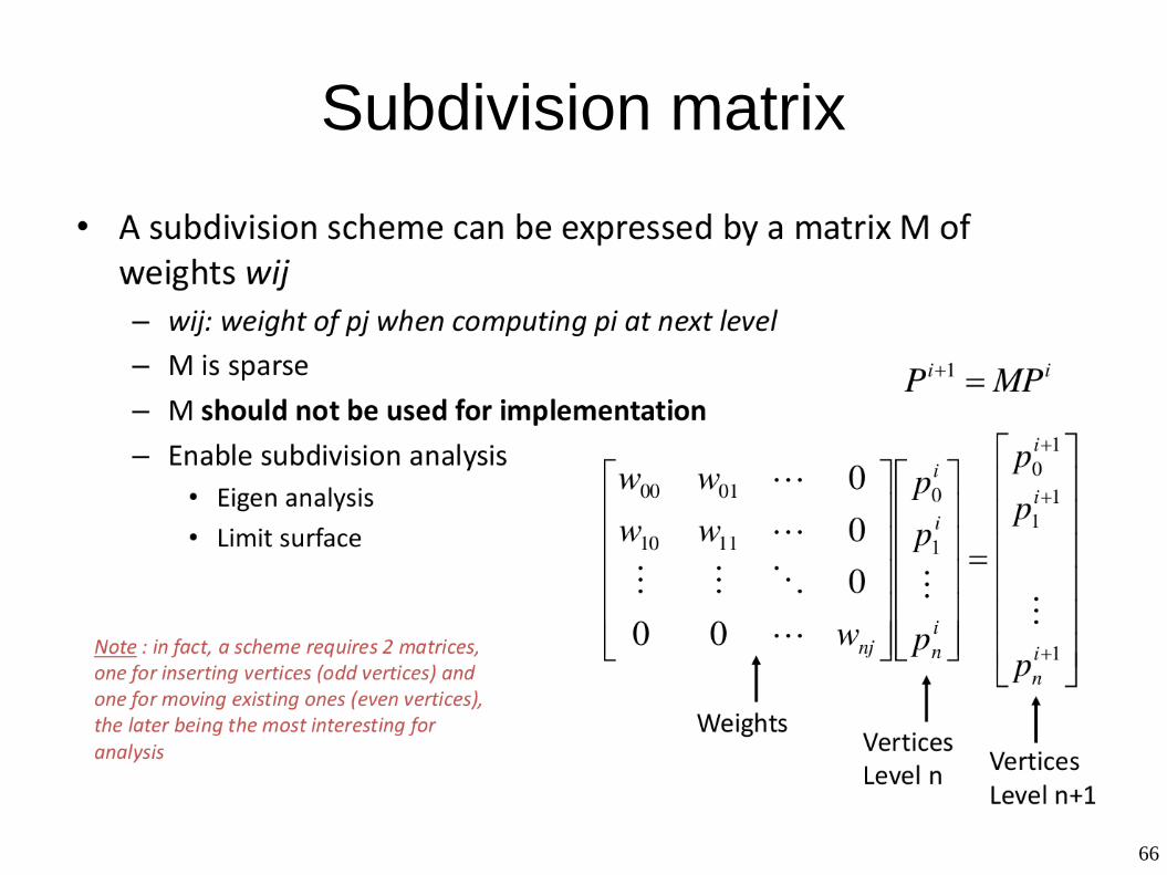
● Modeling-oriented definition(s) and example(s) of :– Curves– Surfaces
● Previously :– Differential Geometry (curves and surfaces in
math)– Meshes (raw representation of surfaces in CS)
3
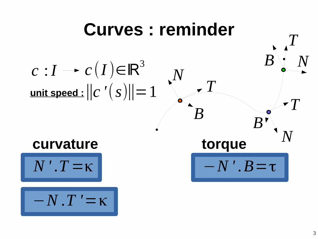
Curves : reminder
c : I c (I )∈ℝ3
TT
T
N
N
N
BB
B
unit speed :‖c '(s)‖=1
torque
N ' .T=κ
−N .T '=κ
−N ' .B=τ
curvature
4
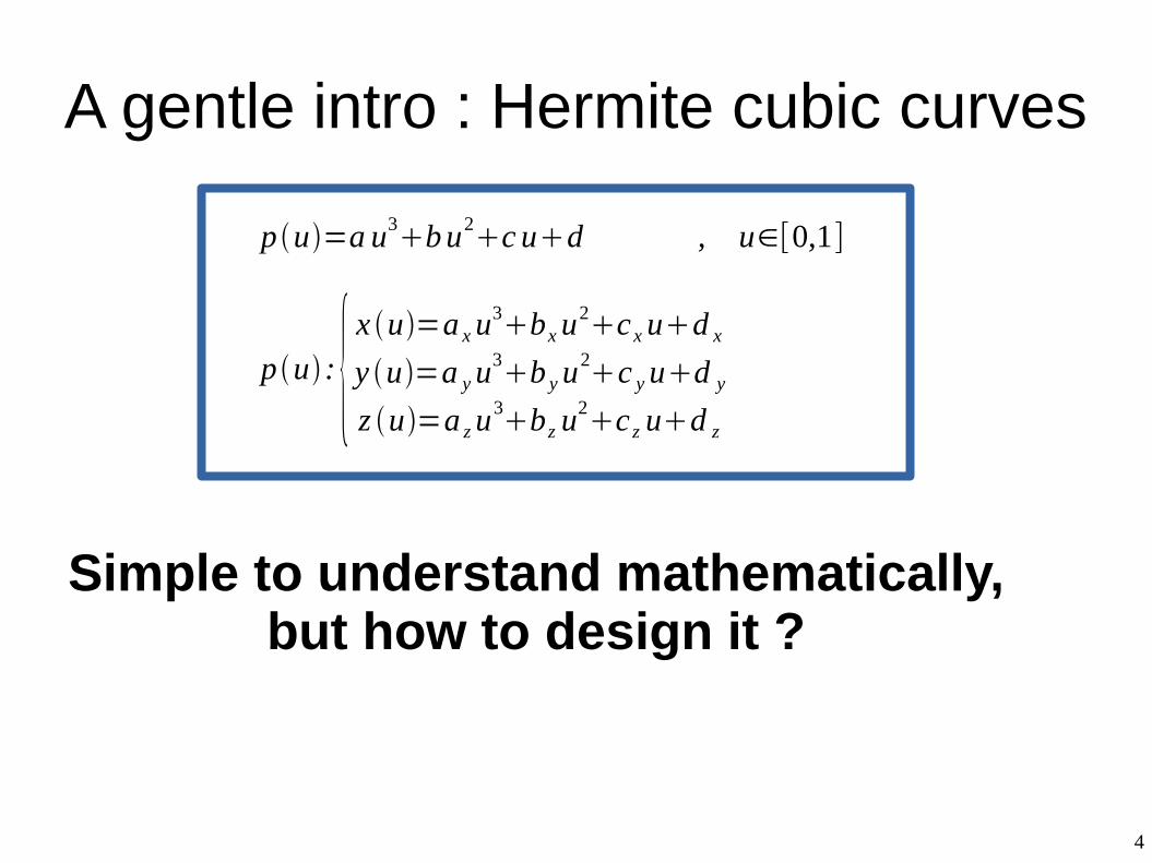
A gentle intro : Hermite cubic curves
p u=a u3bu2c ud , u∈[0,1]
p u :{x u=a xu
3bxu
2c x ud x
y u=a yu3b yu
2c yud y
z u=a zu3bz u
2c z ud z
Simple to understand mathematically, but how to design it ?
5
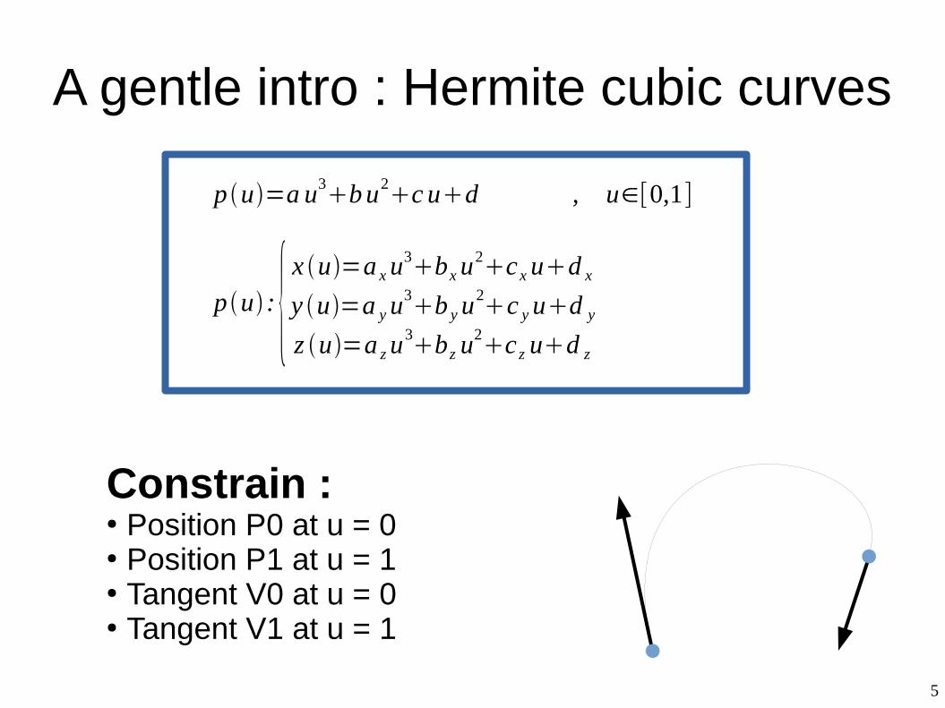
A gentle intro : Hermite cubic curves
p u=a u3bu2c ud , u∈[0,1]
p u :{x u=a xu
3bxu
2c x ud x
y u=a yu3b yu
2c yud y
z u=a zu3bz u
2c z ud z
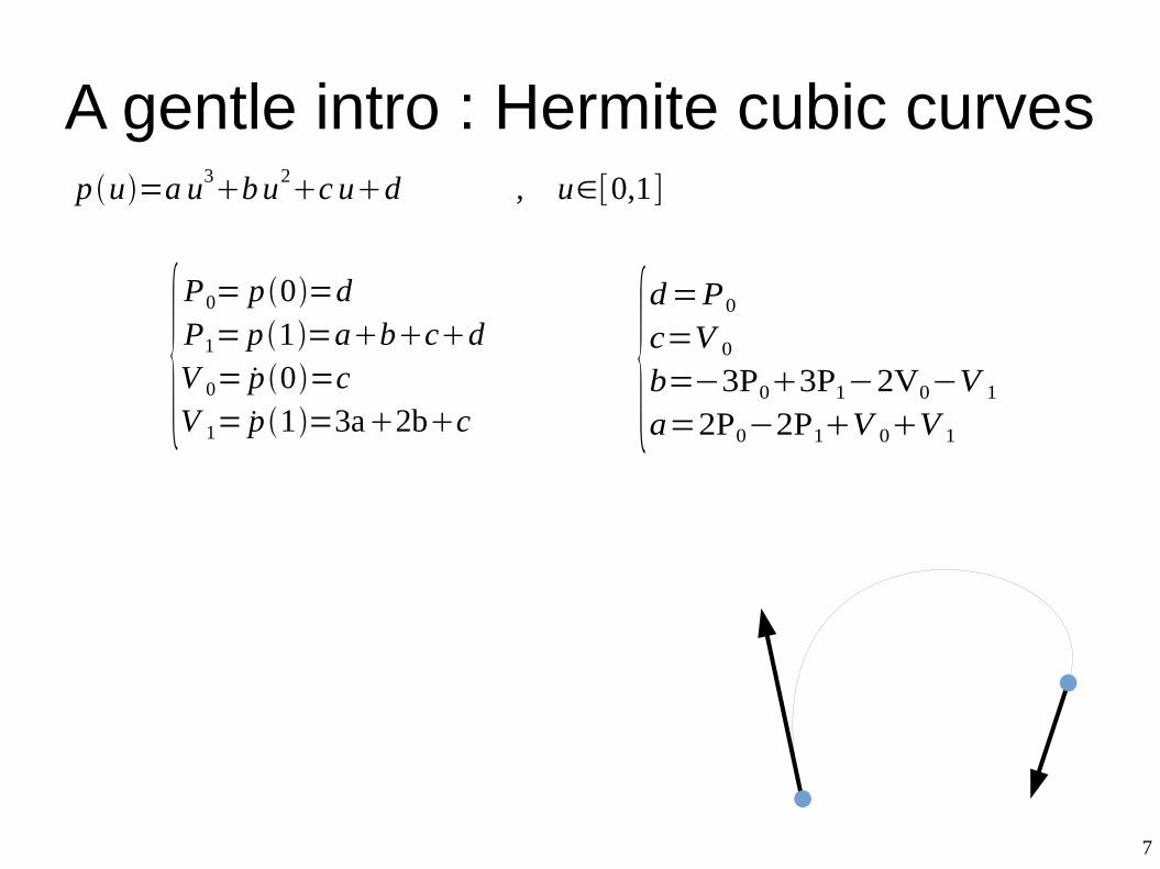
Constrain :● Position P0 at u = 0● Position P1 at u = 1● Tangent V0 at u = 0● Tangent V1 at u = 1
6
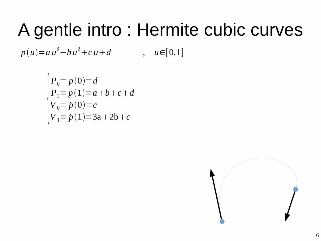
A gentle intro : Hermite cubic curves
{P0= p 0=dP1= p 1=abcdV 0= p 0=cV 1= p 1=3a2bc
p u=a u3bu2c ud , u∈[0,1]
7
A gentle intro : Hermite cubic curves
{P0= p 0=dP1= p 1=abcdV 0= p 0=cV 1= p 1=3a2bc
{d=P0c=V 0
b=−3P03P1−2V0−V 1
a=2P0−2P1V 0V 1
p u=a u3bu2c ud , u∈[0,1]
8
A gentle intro : Hermite cubic curves
{P0= p 0=dP1= p 1=abcdV 0= p 0=cV 1= p 1=3a2bc
{d=P0c=V 0
b=−3P03P1−2V0−V 1
a=2P0−2P1V 0V 1
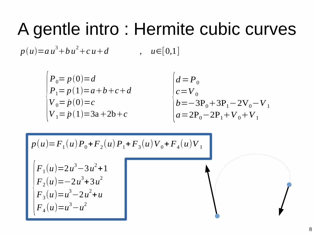
p(u)=F1(u)P0+F2(u)P1+F3(u)V 0+F4(u)V 1
{F1(u)=2u
3−3u2+1
F2(u)=−2u3+3u2
F3(u)=u3−2u2+u
F4 (u)=u3−u2
p u=a u3bu2c ud , u∈[0,1]
9
A gentle intro : Hermite cubic curves
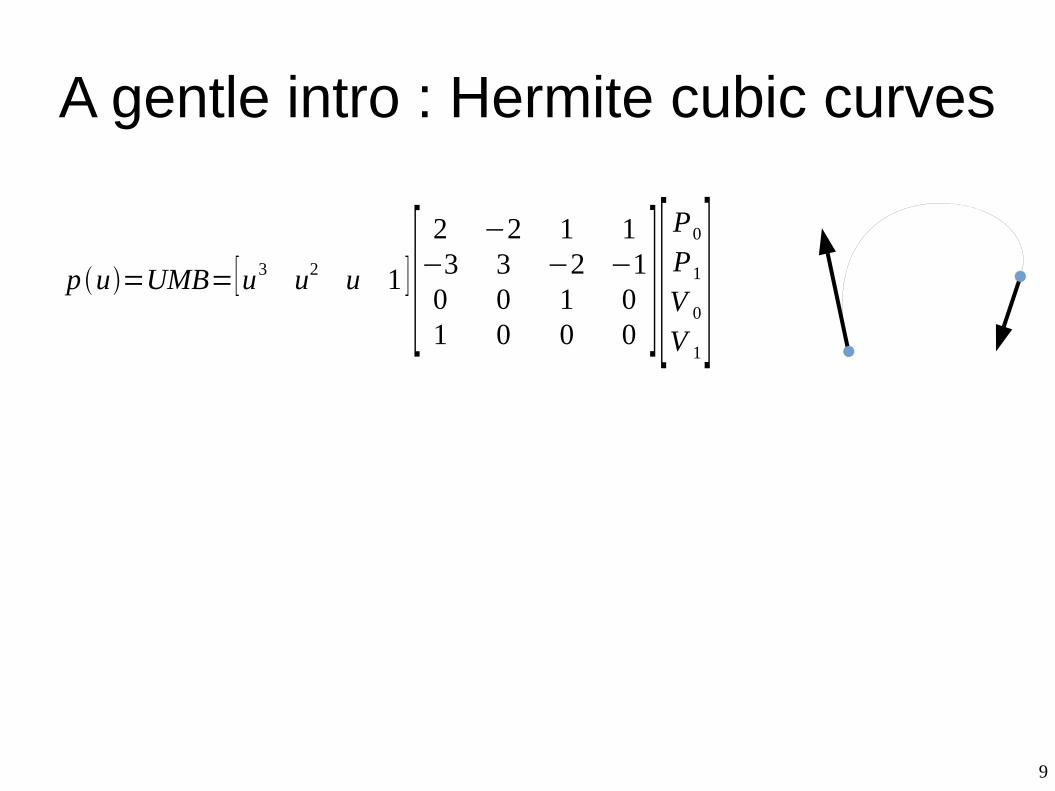
p u=UMB=[u3 u2 u 1 ] [2 −2 1 1
−3 3 −2 −10 0 1 01 0 0 0
][P0P1V 0
V 1]
10
A gentle intro : Hermite cubic curves
p u=UMB=[u3 u2 u 1 ] [2 −2 1 1
−3 3 −2 −10 0 1 01 0 0 0
][P0P1V 0
V 1]
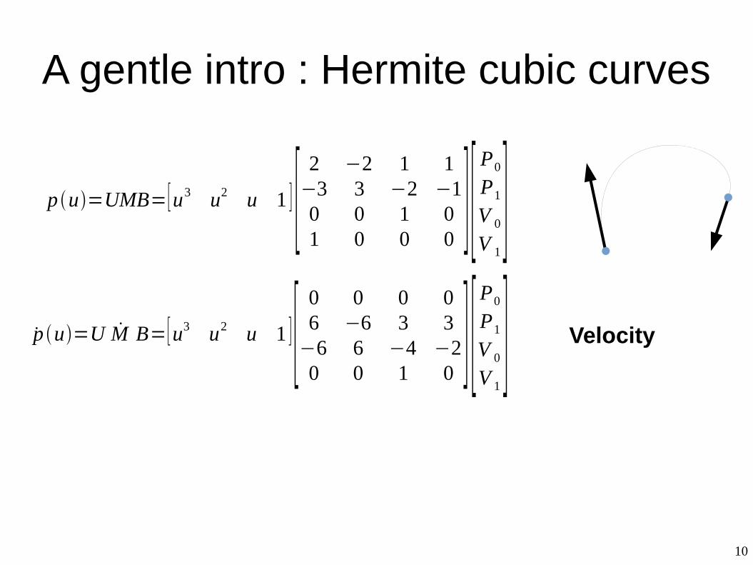
p u=U M B=[u3 u2 u 1 ][0 0 0 06 −6 3 3
−6 6 −4 −20 0 1 0
] [P0P1V 0
V 1] Velocity
11
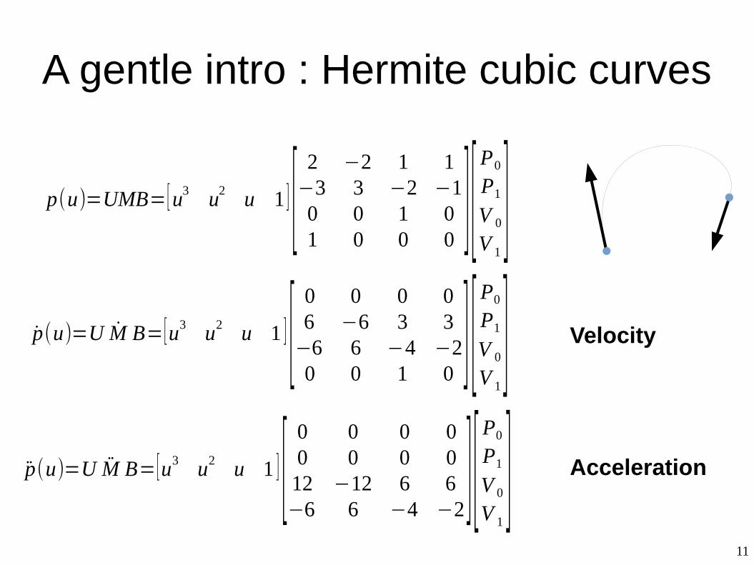
A gentle intro : Hermite cubic curves
p(u)=UMB=[u3 u2 u 1 ] [2 −2 1 1
−3 3 −2 −10 0 1 01 0 0 0
][P0P1V 0
V 1]
p(u)=U M B=[u3 u2 u 1 ] [0 0 0 06 −6 3 3
−6 6 −4 −20 0 1 0
] [P0P1V 0
V 1]
p(u)=U M B=[u3 u2 u 1 ] [0 0 0 00 0 0 012 −12 6 6−6 6 −4 −2
][P0P1V 0V 1
]
Velocity
Acceleration
12
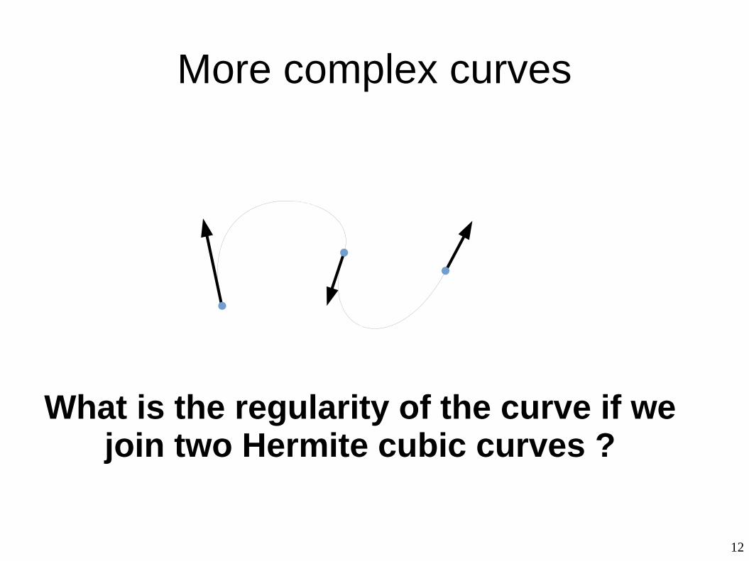
More complex curves
What is the regularity of the curve if we join two Hermite cubic curves ?
13
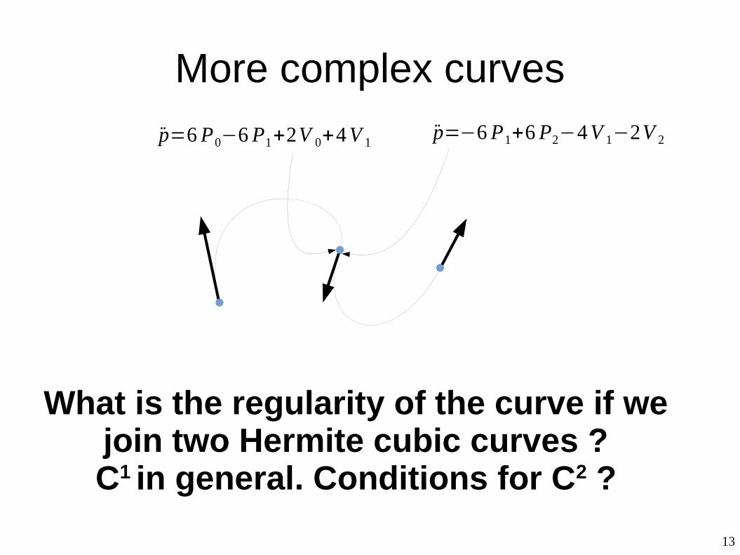
More complex curves
What is the regularity of the curve if we join two Hermite cubic curves ?C1 in general. Conditions for C2 ?
p=6P0−6P1+2V 0+4V 1 p=−6P1+6P2−4V 1−2V 2
14
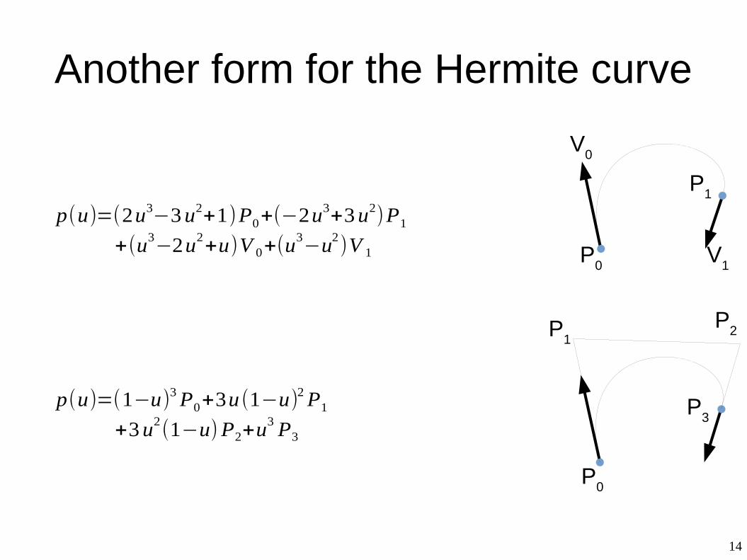
Another form for the Hermite curve
P0
V0
P1
V1
P0
P1
P2
P3
p(u)=(2u3−3u2+1)P0+(−2u3+3u2)P1+(u3−2u2+u)V 0+(u3−u2)V 1
p(u)=(1−u)3P0+3u (1−u)2P1
+3u2(1−u)P2+u3 P3
15
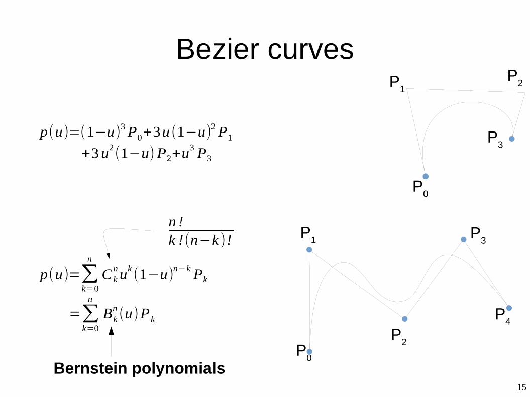
Bezier curves
P0
P1
P2
P3
p(u)=(1−u)3P0+3u (1−u)2P1
+3u2(1−u)P2+u3 P3
p(u)=∑k=0
n
C knuk (1−u)n−k Pk
=∑k=0
n
Bkn(u)Pk
P0
P1
P2
P3
P4
Bernstein polynomials
n !k !(n−k )!
16
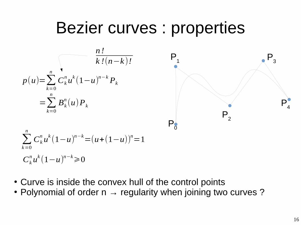
Bezier curves : properties
p(u)=∑k=0
n
C knuk (1−u)n−k Pk
=∑k=0
n
Bkn(u)Pk
P0
P1
P2
P3
P4
n !k !(n−k )!
∑k=0
n
C kn uk (1−u)n−k=(u+(1−u))n=1
C knuk (1−u)n−k⩾0
● Curve is inside the convex hull of the control points● Polynomial of order n → regularity when joining two curves ?
17
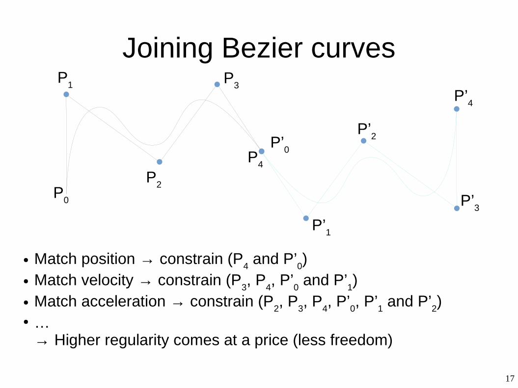
Joining Bezier curves
P0
P1
P2
P3
P4
P’0
P’1
P’2
P’3
P’4
● Match position → constrain (P4 and P’
0)
● Match velocity → constrain (P3, P
4, P’
0 and P’
1)
● Match acceleration → constrain (P2, P
3, P
4, P’
0, P’
1 and P’
2)
● …→ Higher regularity comes at a price (less freedom)
18
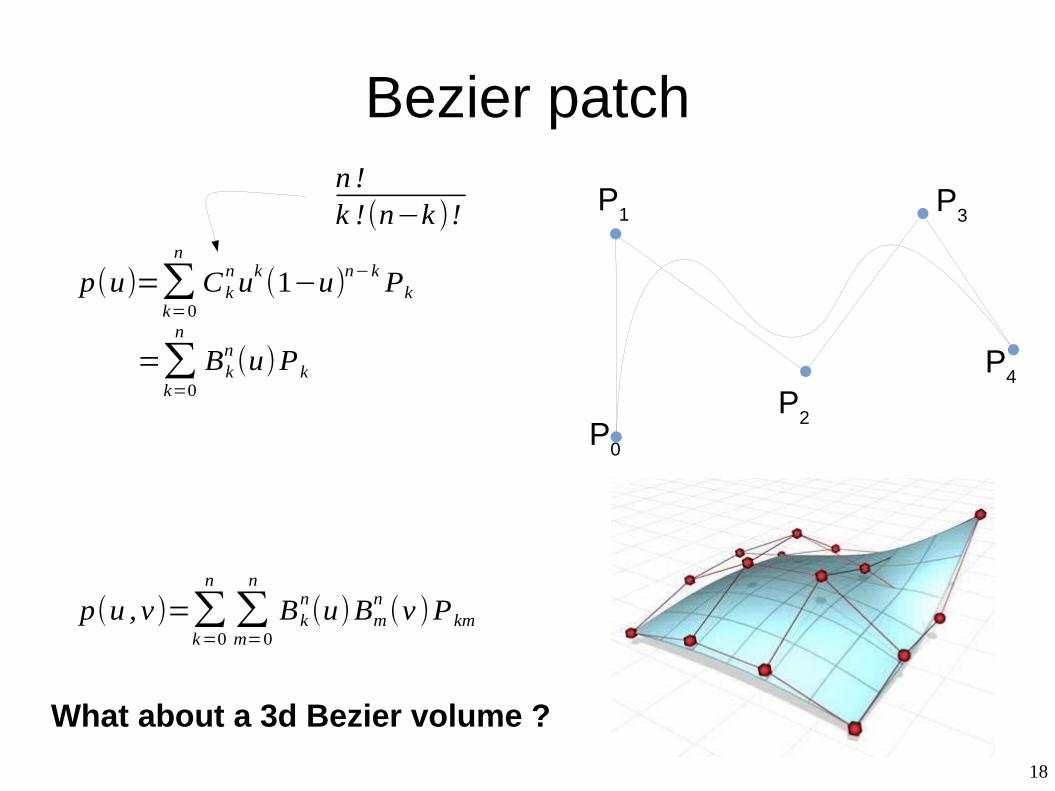
Bezier patch
p(u)=∑k=0
n
C knuk (1−u)n−k Pk
=∑k=0
n
Bkn(u)Pk
P0
P1
P2
P3
P4
n !k !(n−k )!
p(u , v)=∑k=0
n
∑m=0
n
Bkn(u)Bm
n(v )Pkm
What about a 3d Bezier volume ?
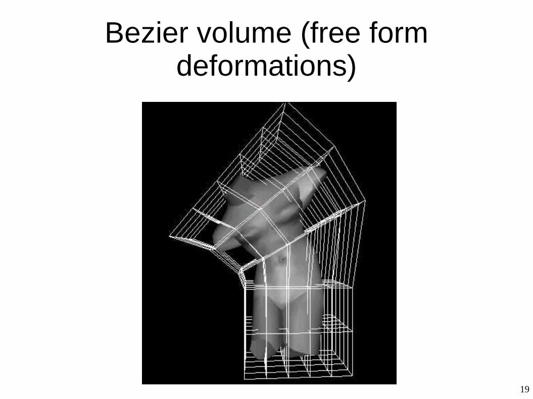
19
Bezier volume (free form deformations)
20
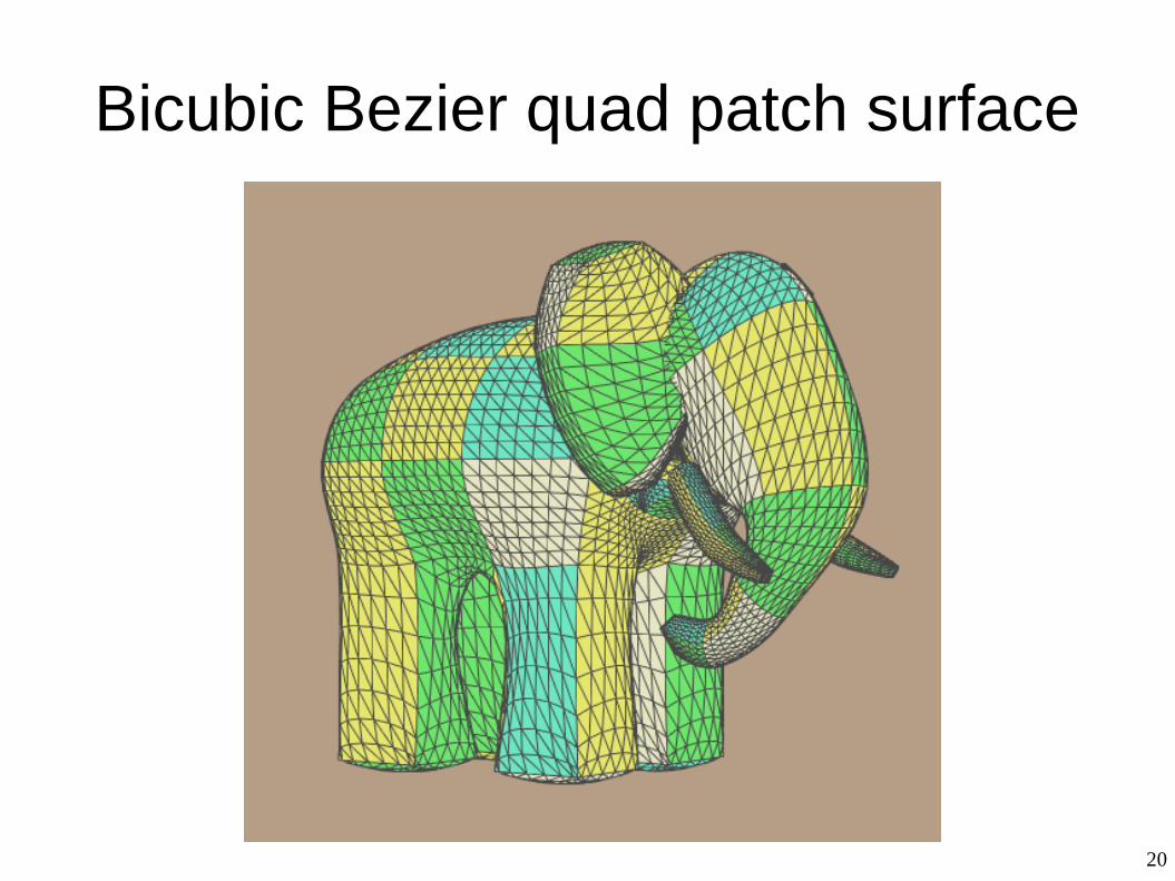
Bicubic Bezier quad patch surface
21
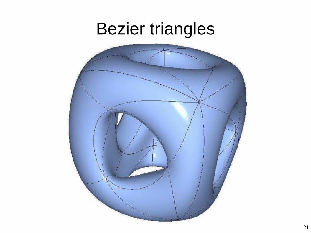
Bezier triangles
22
Bezier triangles
23
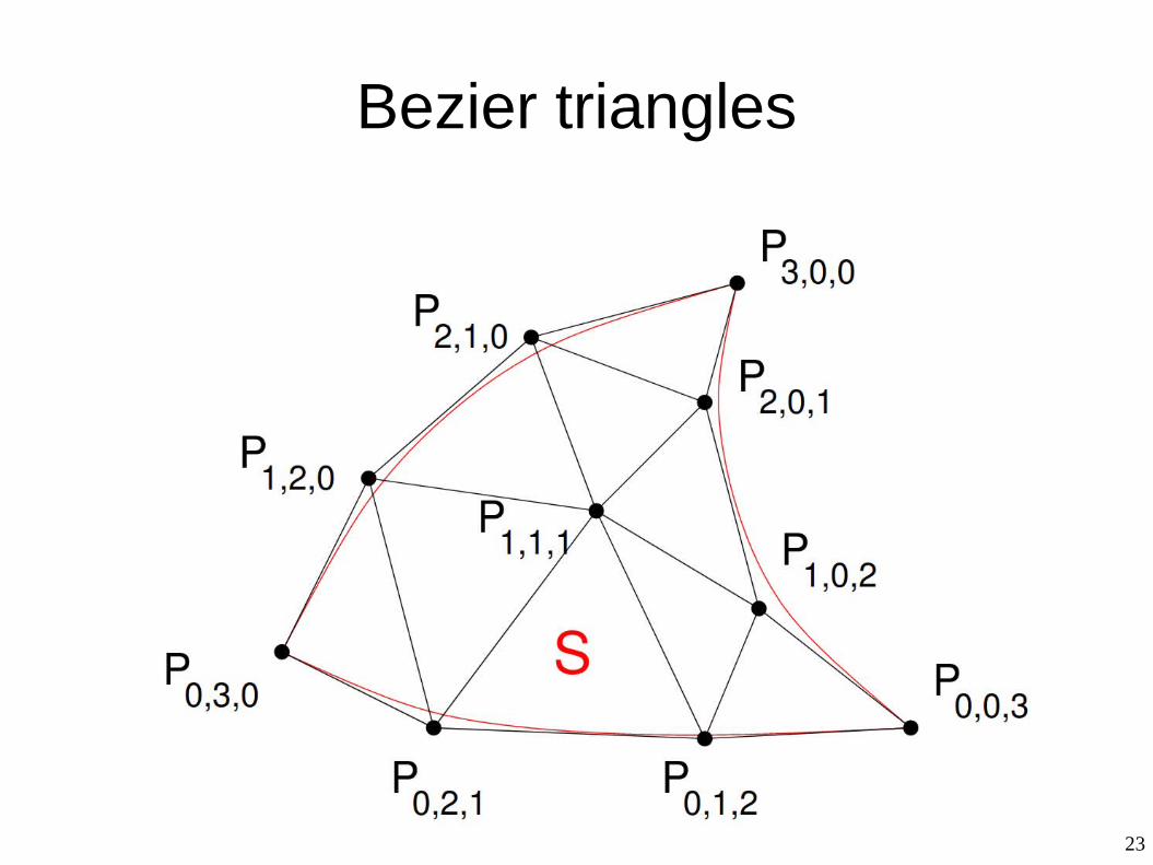
Bezier triangles
24
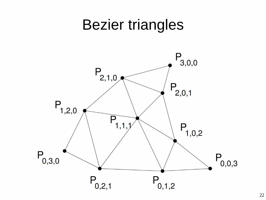
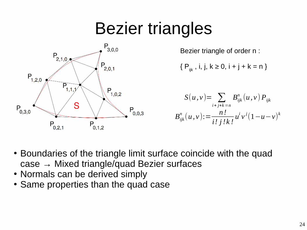
Bezier trianglesBezier triangle of order n :
{ Pijk , i, j, k ≥ 0, i + j + k = n }
S(u , v )= ∑i+ j+k=n
Bijkn (u , v )Pijk
Bijkn(u , v ):=
n !i! j !k !
ui v j(1−u−v)k
● Boundaries of the triangle limit surface coincide with the quad case → Mixed triangle/quad Bezier surfaces
● Normals can be derived simply● Same properties than the quad case
25
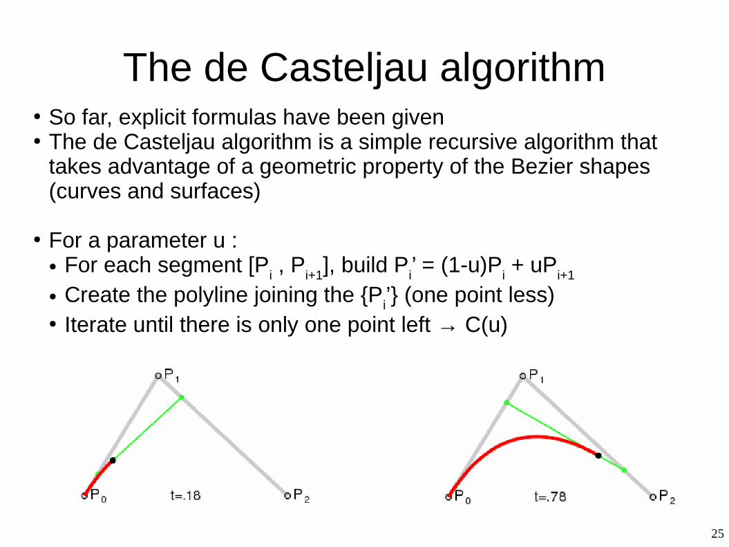
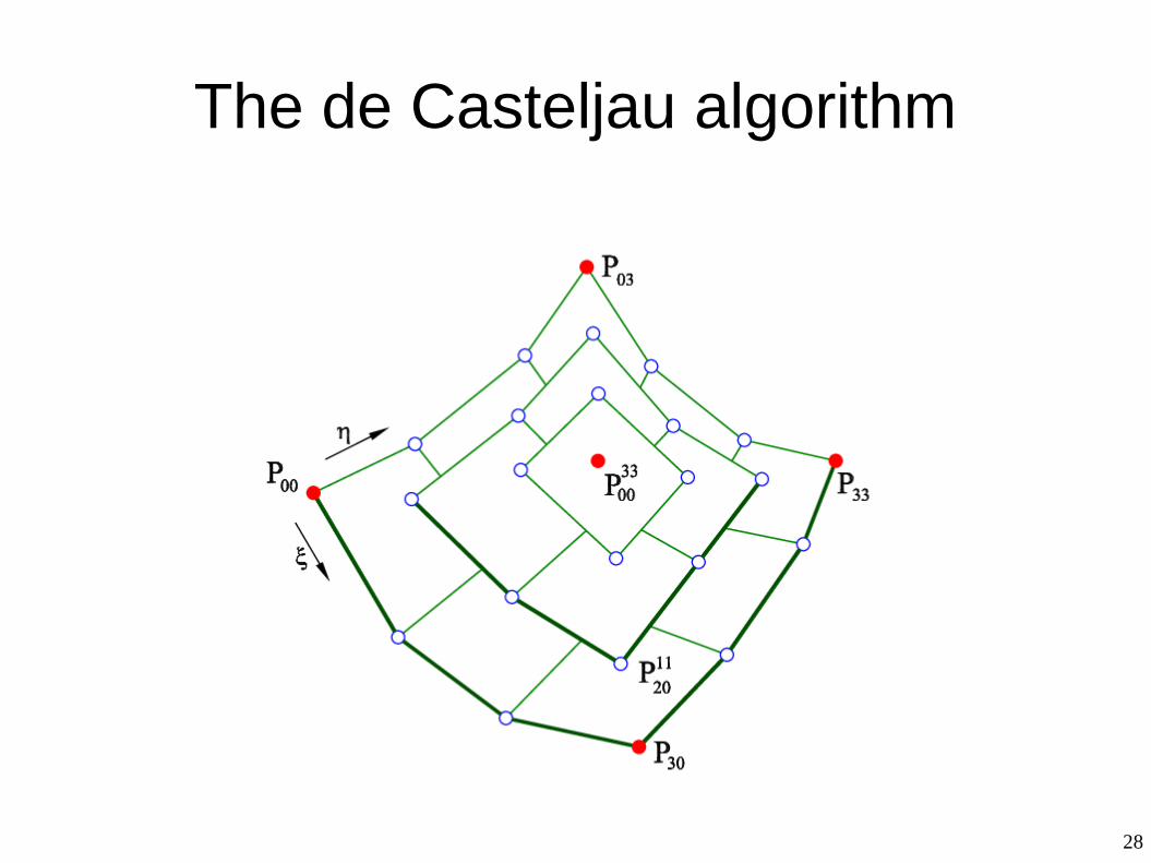
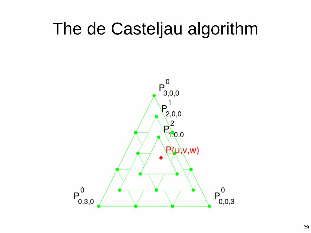
The de Casteljau algorithm● So far, explicit formulas have been given● The de Casteljau algorithm is a simple recursive algorithm that
takes advantage of a geometric property of the Bezier shapes (curves and surfaces)
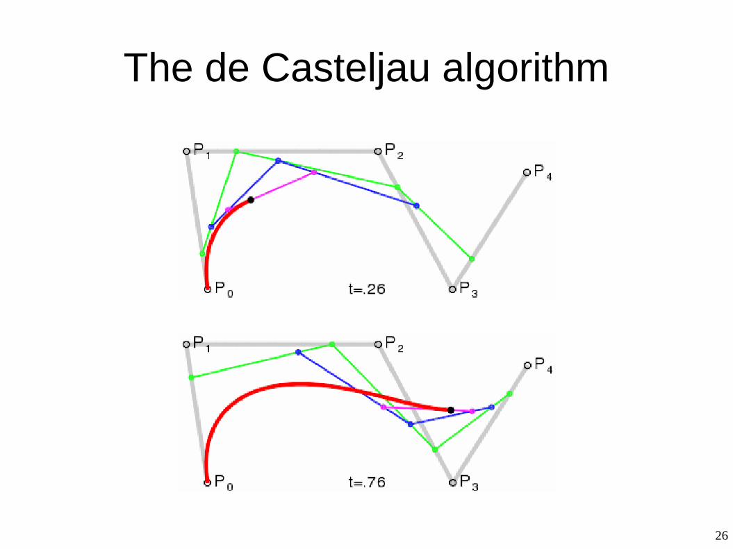
● For a parameter u :● For each segment [P
i , P
i+1], build P
i’ = (1-u)P
i + uP
i+1
● Create the polyline joining the {Pi’} (one point less)
● Iterate until there is only one point left → C(u)
26
The de Casteljau algorithm
27
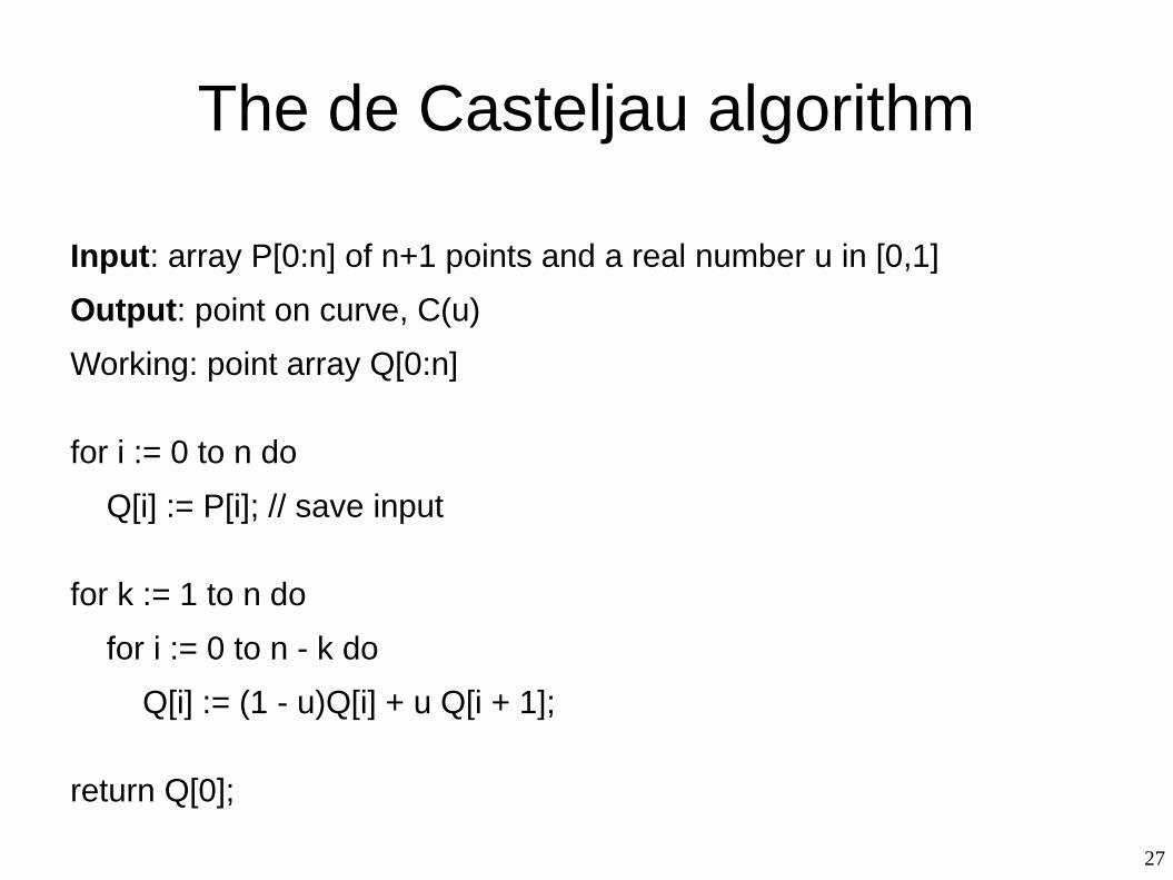
The de Casteljau algorithm
Input: array P[0:n] of n+1 points and a real number u in [0,1]
Output: point on curve, C(u)
Working: point array Q[0:n]
for i := 0 to n do
Q[i] := P[i]; // save input
for k := 1 to n do
for i := 0 to n - k do
Q[i] := (1 - u)Q[i] + u Q[i + 1];
return Q[0];
28
The de Casteljau algorithm
29
The de Casteljau algorithm
30
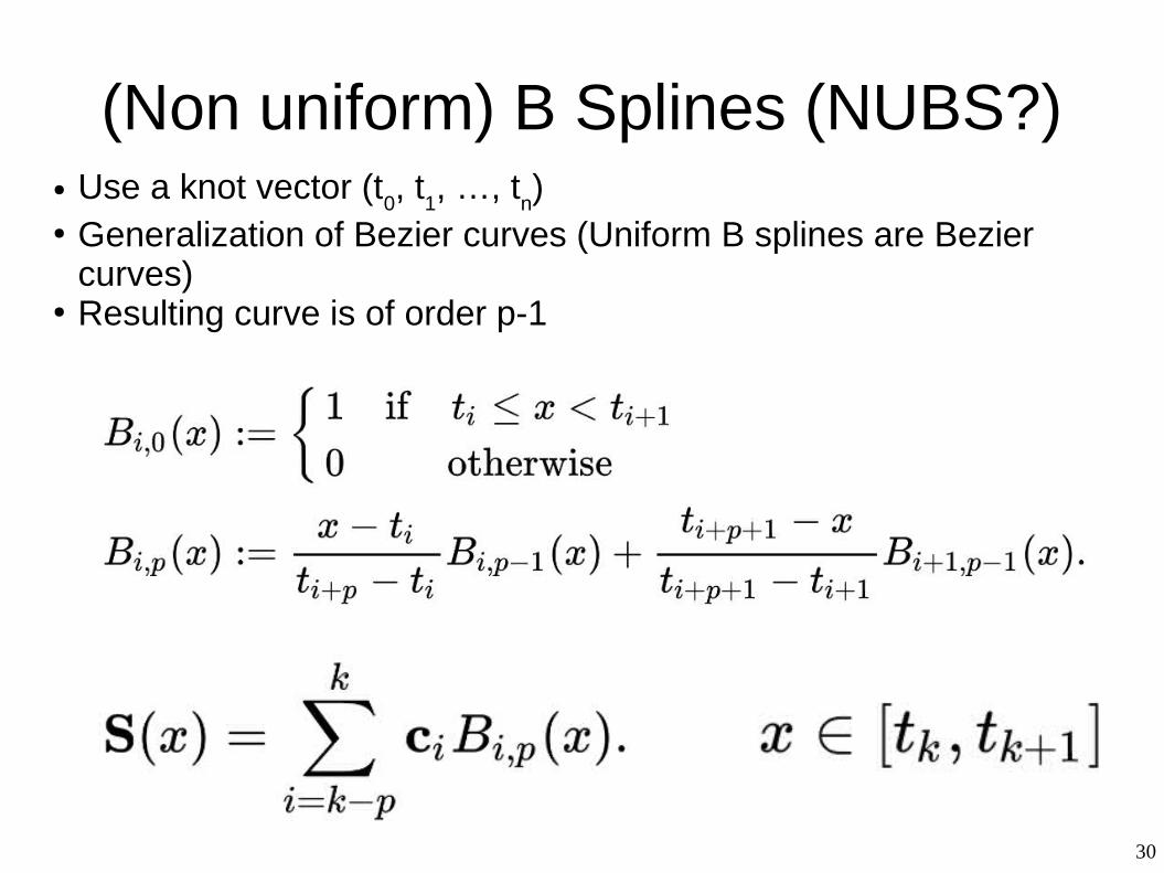
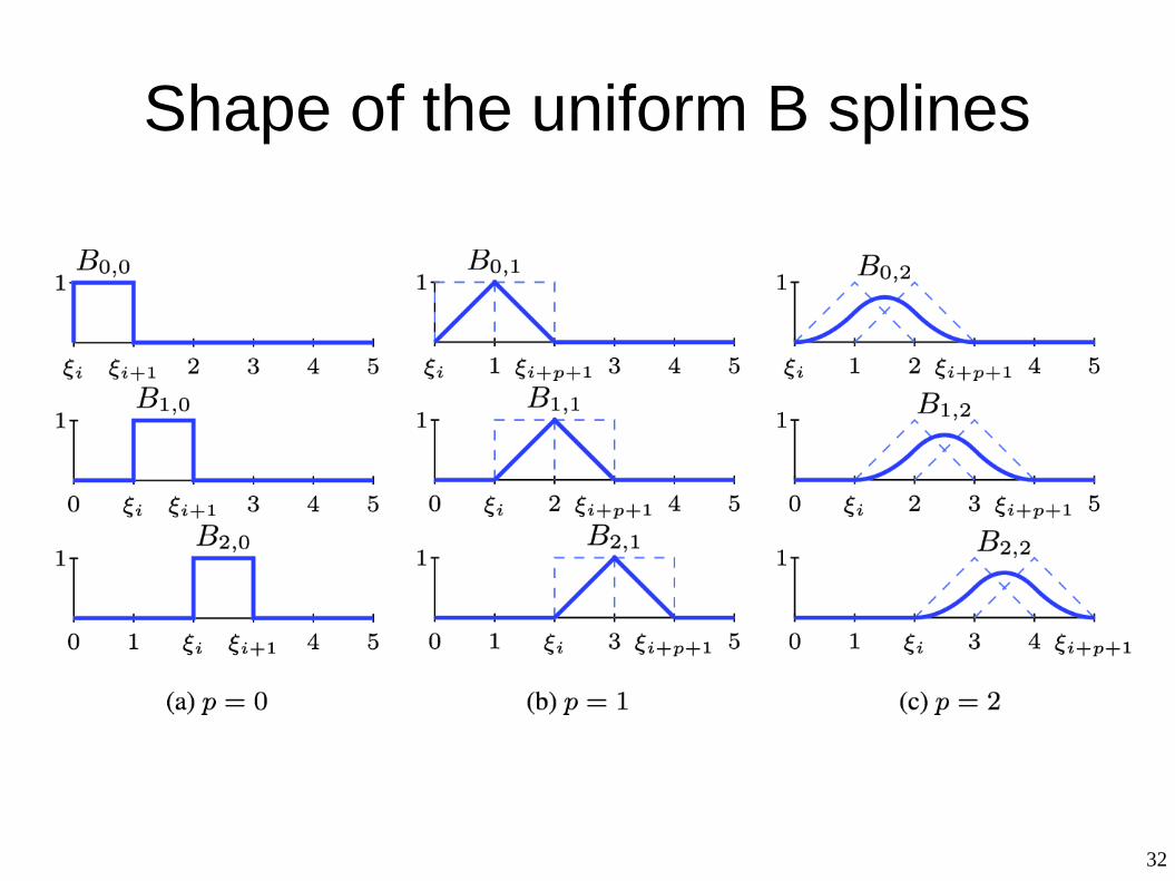
(Non uniform) B Splines (NUBS?)● Use a knot vector (t
0, t
1, …, t
n)
● Generalization of Bezier curves (Uniform B splines are Bezier curves)
● Resulting curve is of order p-1
32
Shape of the uniform B splines
33
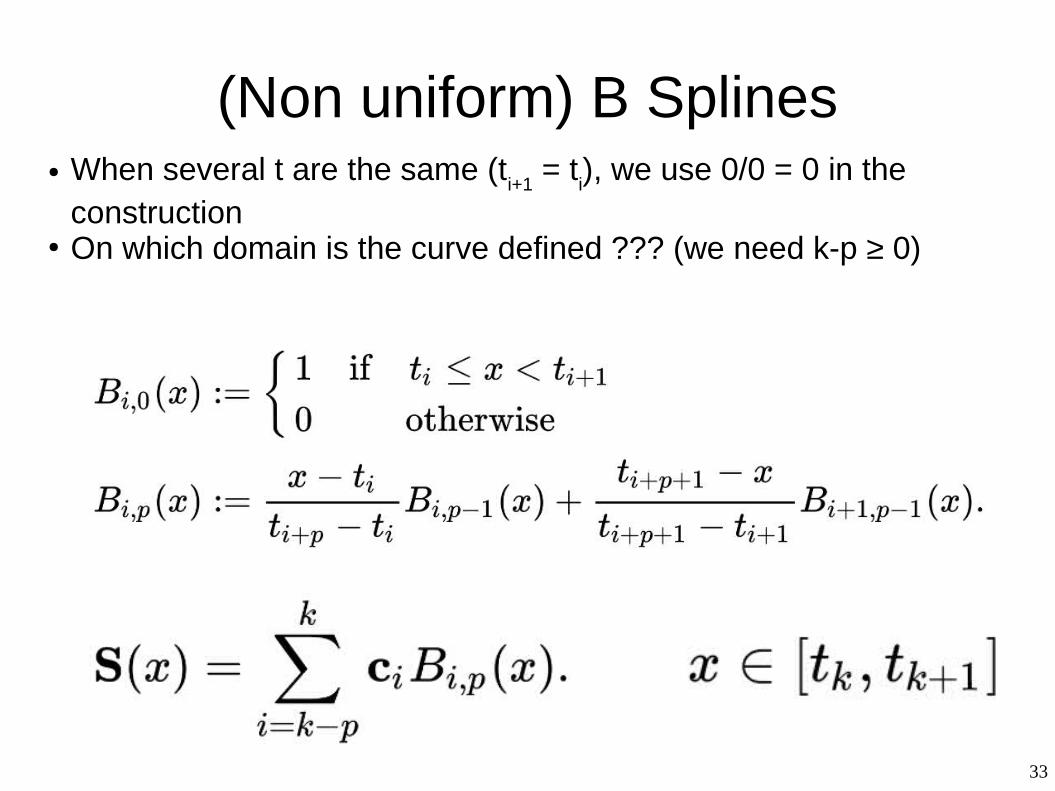
(Non uniform) B Splines● When several t are the same (t
i+1 = t
i), we use 0/0 = 0 in the
construction● On which domain is the curve defined ??? (we need k-p ≥ 0)
34
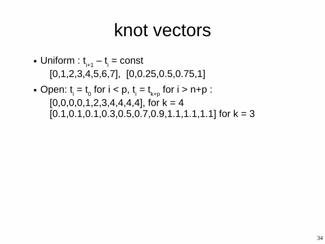
knot vectors
● Uniform : ti+1
– ti = const
[0,1,2,3,4,5,6,7], [0,0.25,0.5,0.75,1]
● Open: ti = t
0 for i < p, t
i = t
k+p for i > n+p :
[0,0,0,0,1,2,3,4,4,4,4], for k = 4[0.1,0.1,0.1,0.3,0.5,0.7,0.9,1.1,1.1,1.1] for k = 3
35
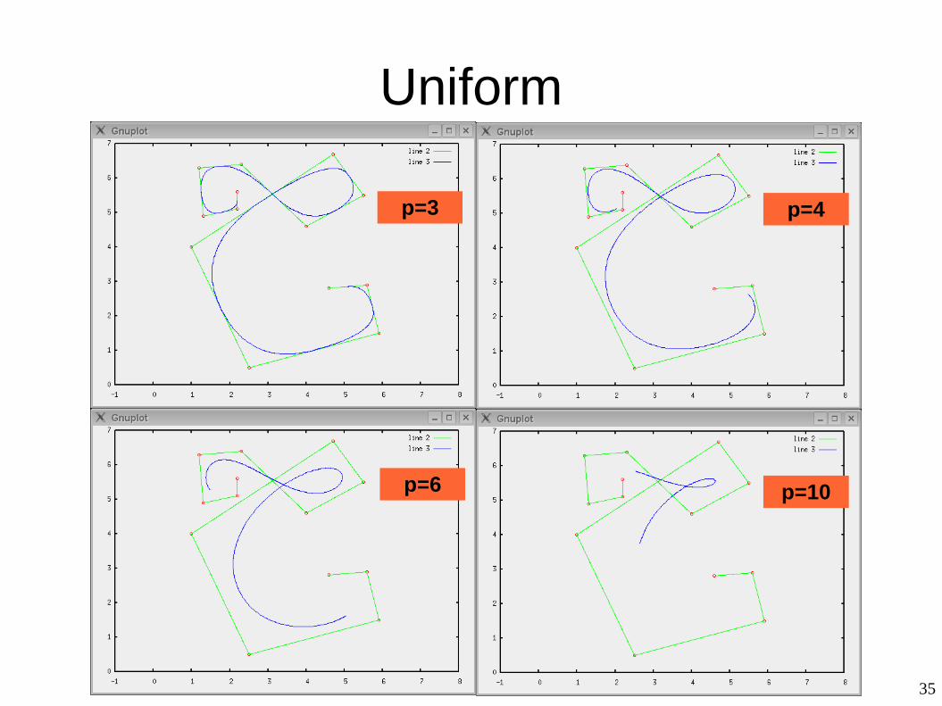
Uniform
p=3 p=4
p=6 p=10
36
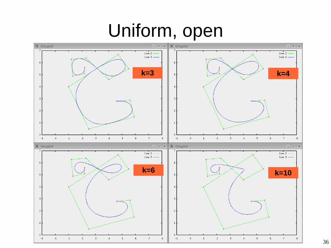
Uniform, open
k=3 k=4
k=6 k=10
37
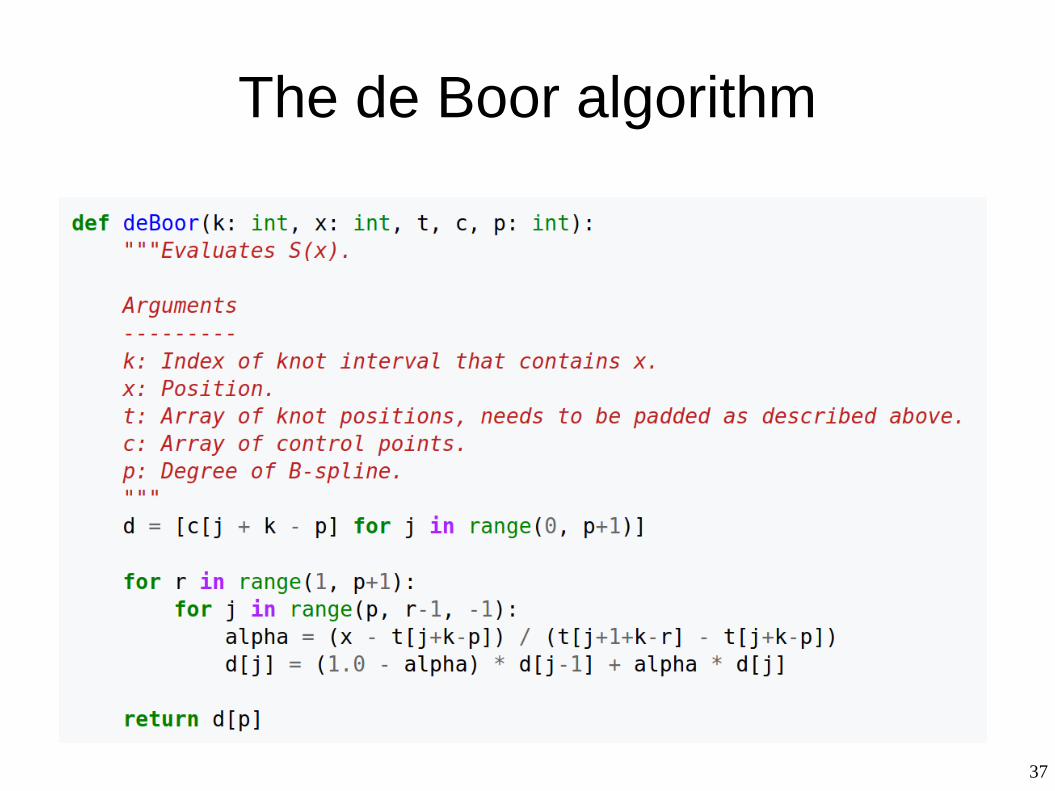
The de Boor algorithm
38
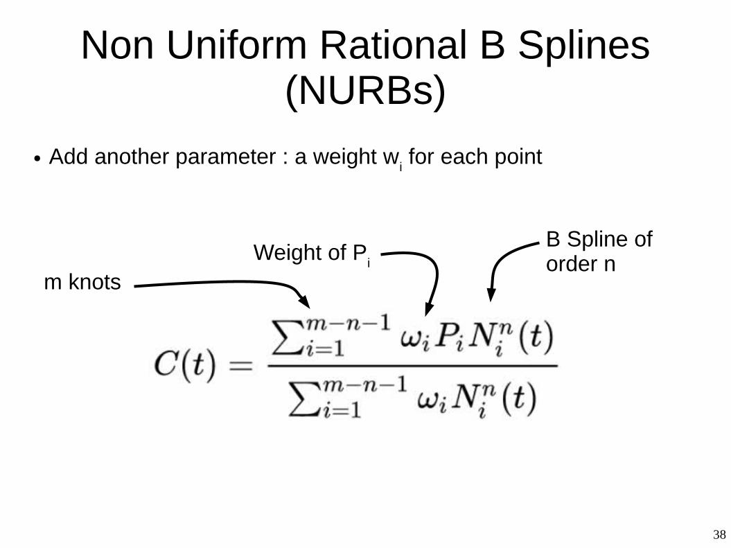
Non Uniform Rational B Splines (NURBs)
● Add another parameter : a weight wi for each point
B Spline of order nWeight of P
i
m knots
39
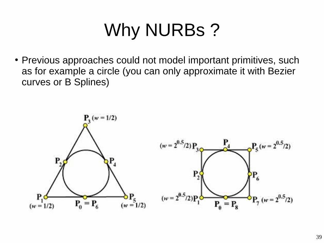
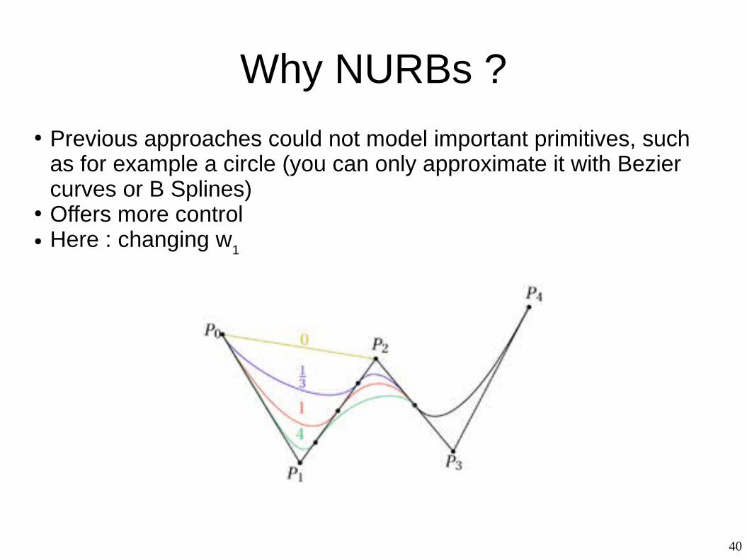
Why NURBs ?● Previous approaches could not model important primitives, such
as for example a circle (you can only approximate it with Bezier curves or B Splines)
40
Why NURBs ?● Previous approaches could not model important primitives, such
as for example a circle (you can only approximate it with Bezier curves or B Splines)
● Offers more control● Here : changing w
1
41
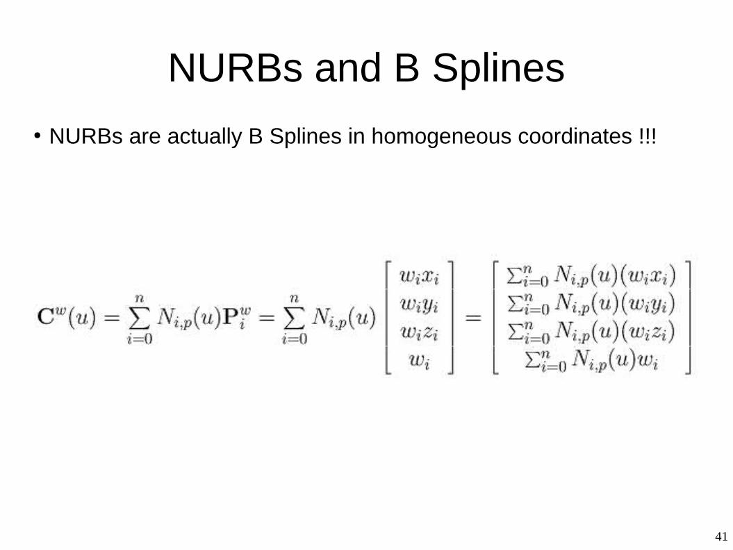
NURBs and B Splines● NURBs are actually B Splines in homogeneous coordinates !!!
42
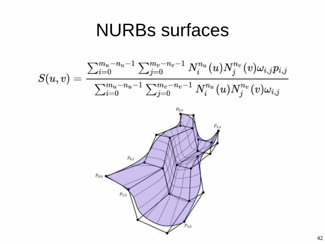
NURBs surfaces
43
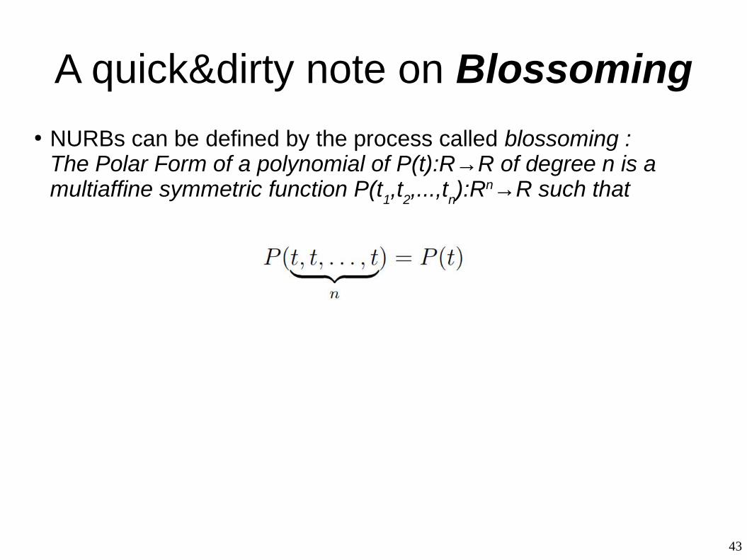
A quick&dirty note on Blossoming● NURBs can be defined by the process called blossoming :
The Polar Form of a polynomial of P(t):R→R of degree n is a multiaffine symmetric function P(t
1,t
2,...,t
n):Rn→R such that
44
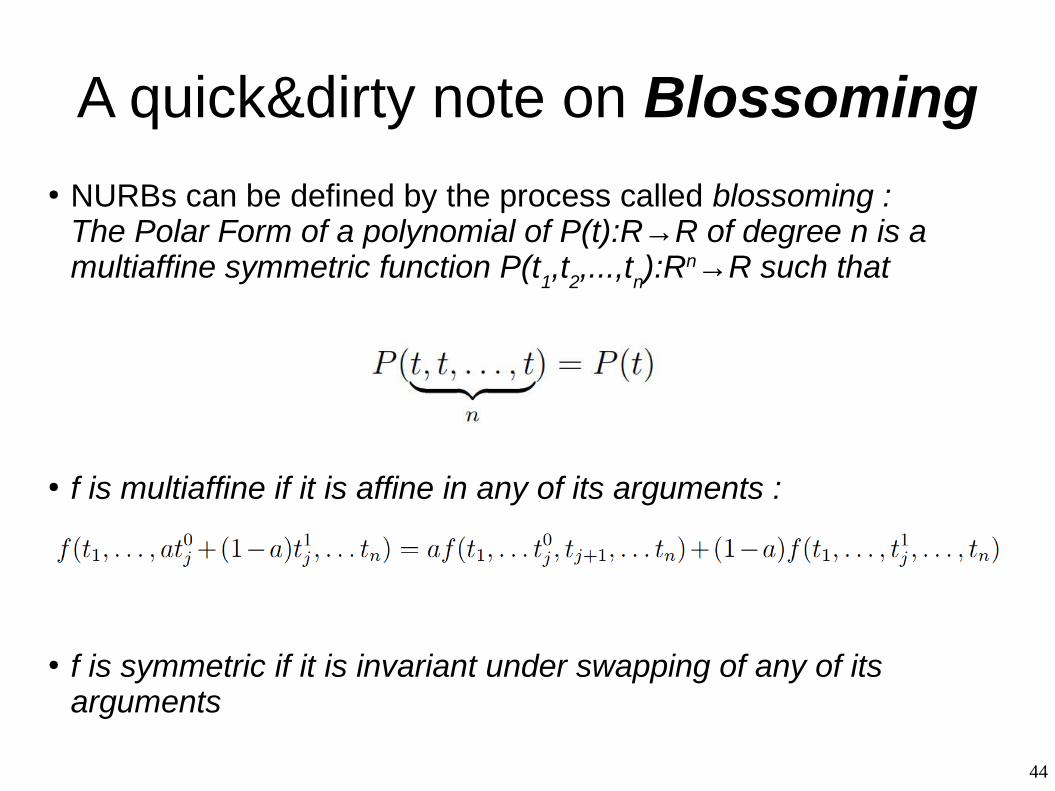
A quick&dirty note on Blossoming● NURBs can be defined by the process called blossoming :
The Polar Form of a polynomial of P(t):R→R of degree n is a multiaffine symmetric function P(t
1,t
2,...,t
n):Rn→R such that
● f is multiaffine if it is affine in any of its arguments :
● f is symmetric if it is invariant under swapping of any of its arguments
45
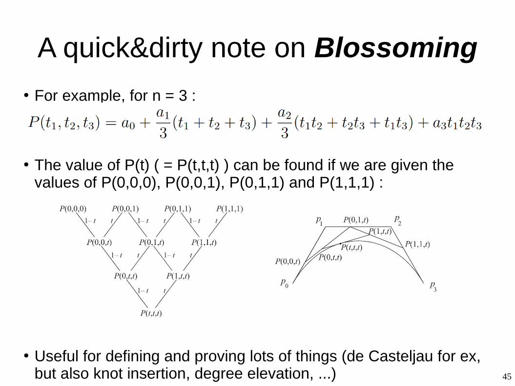
A quick&dirty note on Blossoming● For example, for n = 3 :
● The value of P(t) ( = P(t,t,t) ) can be found if we are given the values of P(0,0,0), P(0,0,1), P(0,1,1) and P(1,1,1) :
● Useful for defining and proving lots of things (de Casteljau for ex, but also knot insertion, degree elevation, ...)

46
A quick&dirty note on Automata● Blossoming can also be understood as a form of automata
The quadratic NURBS CIFS-automaton
The cubic NURBS CIFS-automaton
47
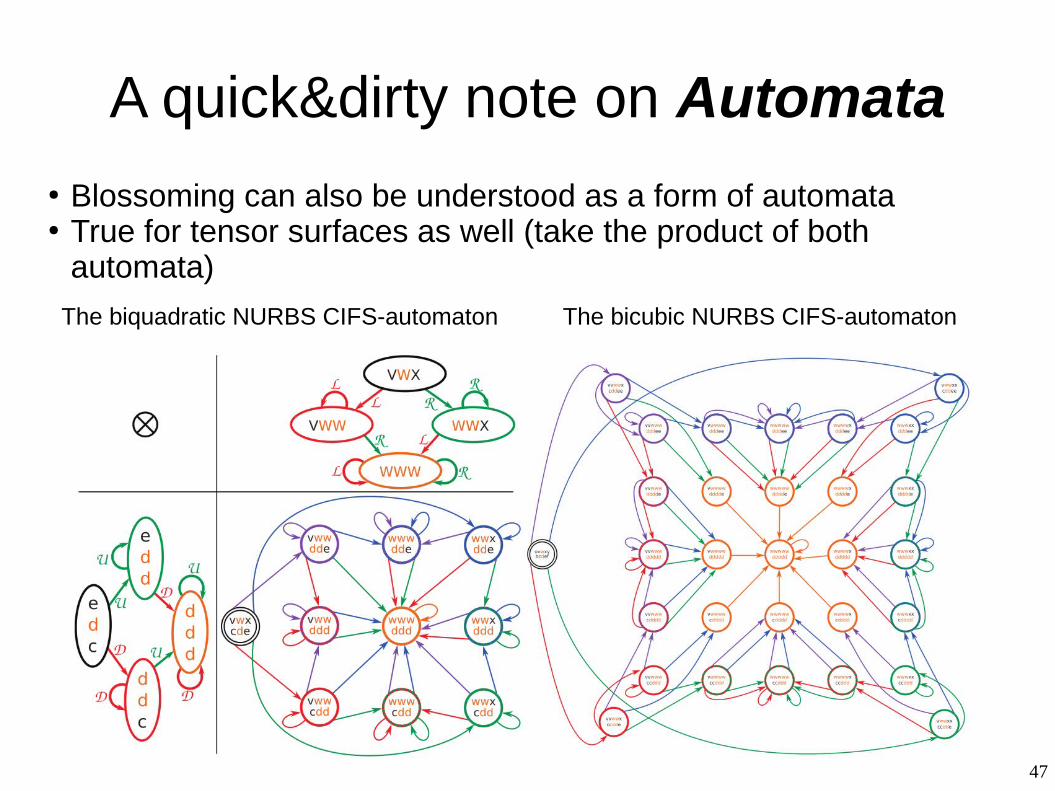
A quick&dirty note on Automata● Blossoming can also be understood as a form of automata● True for tensor surfaces as well (take the product of both
automata)
The biquadratic NURBS CIFS-automaton The bicubic NURBS CIFS-automaton
48
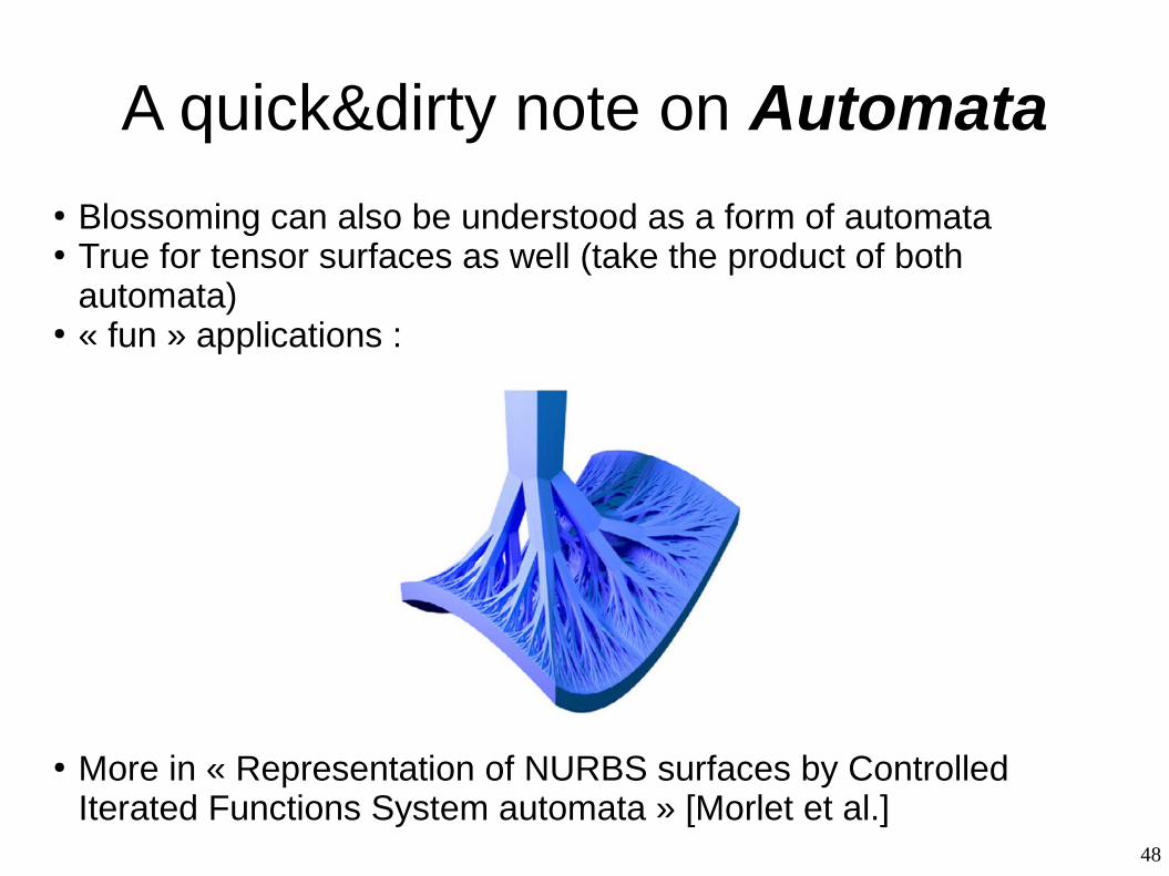
A quick&dirty note on Automata● Blossoming can also be understood as a form of automata● True for tensor surfaces as well (take the product of both
automata)● « fun » applications :
● More in « Representation of NURBS surfaces by Controlled Iterated Functions System automata » [Morlet et al.]

49
Summary● Curves
● Bezier● B Splines● NURBs
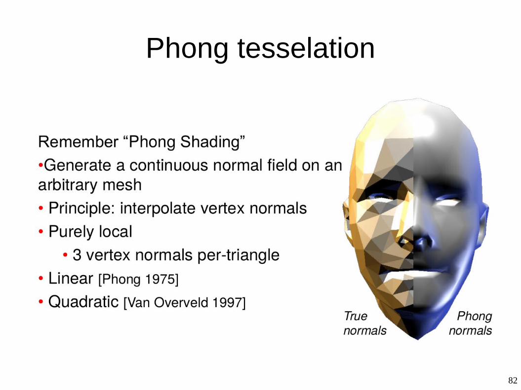
● Surfaces● Bezier (triangle, quad)● B Splines (quad)● NURBs (quad)● PN triangles (see later)● Phong patches (see later)● Coon patches (not seen here)● And more and more and more…
● Which model should we use ???
50
Subdivision surfaces● All models previously seen are nice, but are complex to use, not
easy to implement efficiently, complex to interact with…● Splines were the major standard in the 70s● Subdivision surfaces appeared after that to propose a more simple
mechanism.
51
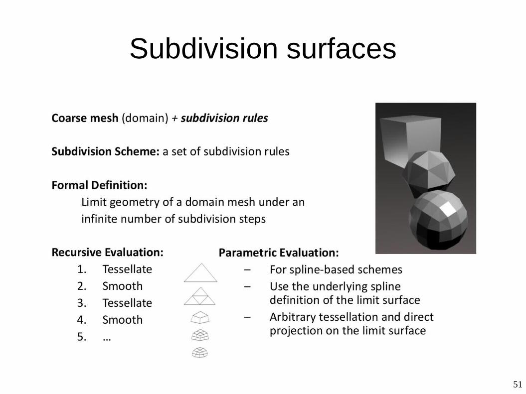
Subdivision surfaces
52
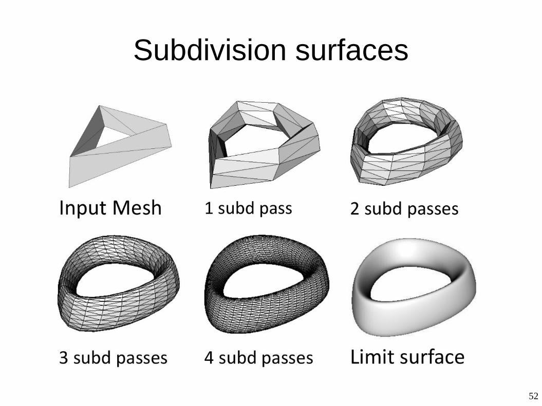
Subdivision surfaces
53
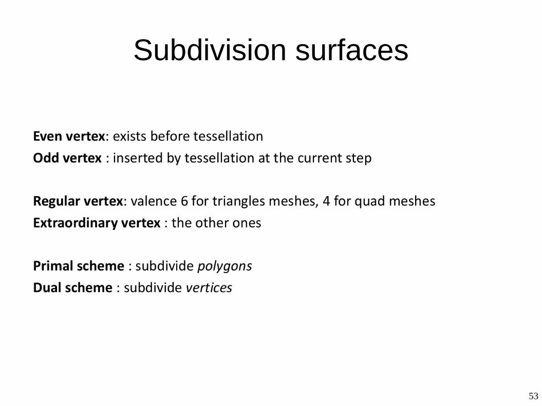
Subdivision surfaces
54
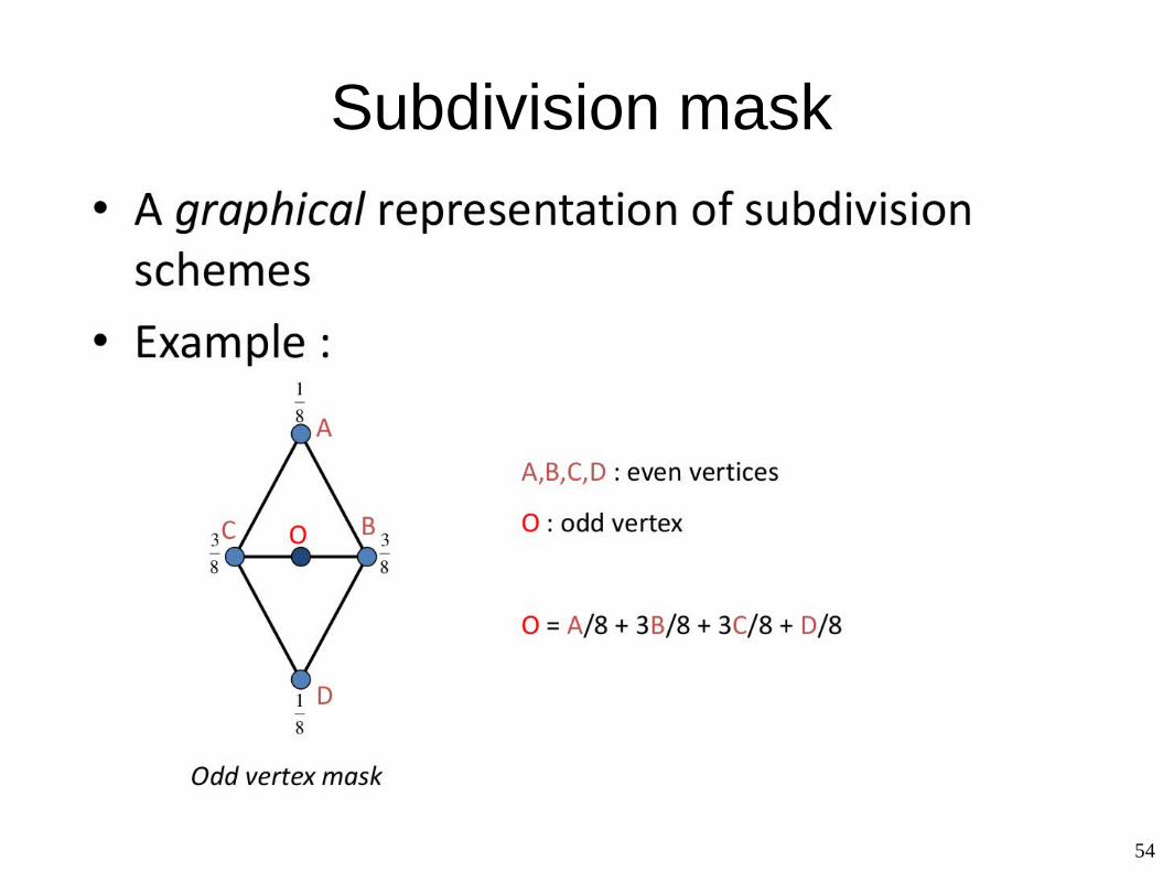
Subdivision mask
55
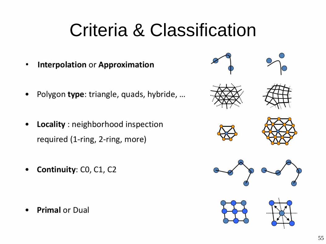
Criteria & Classification
56
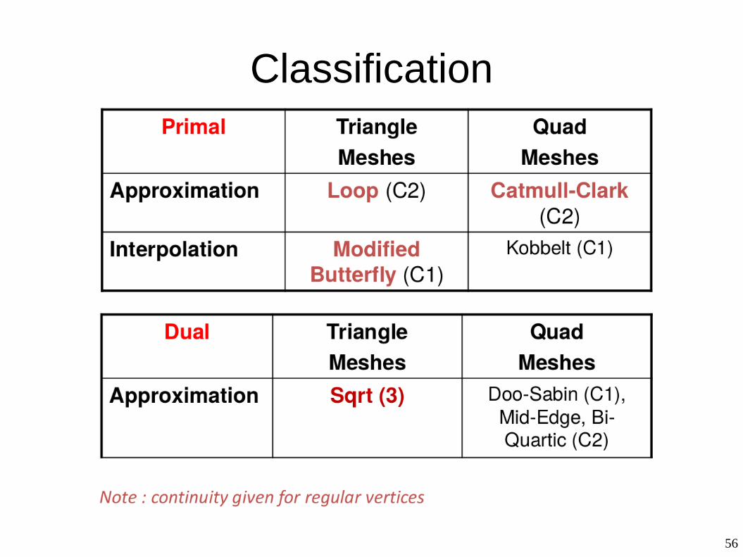
Classification
57
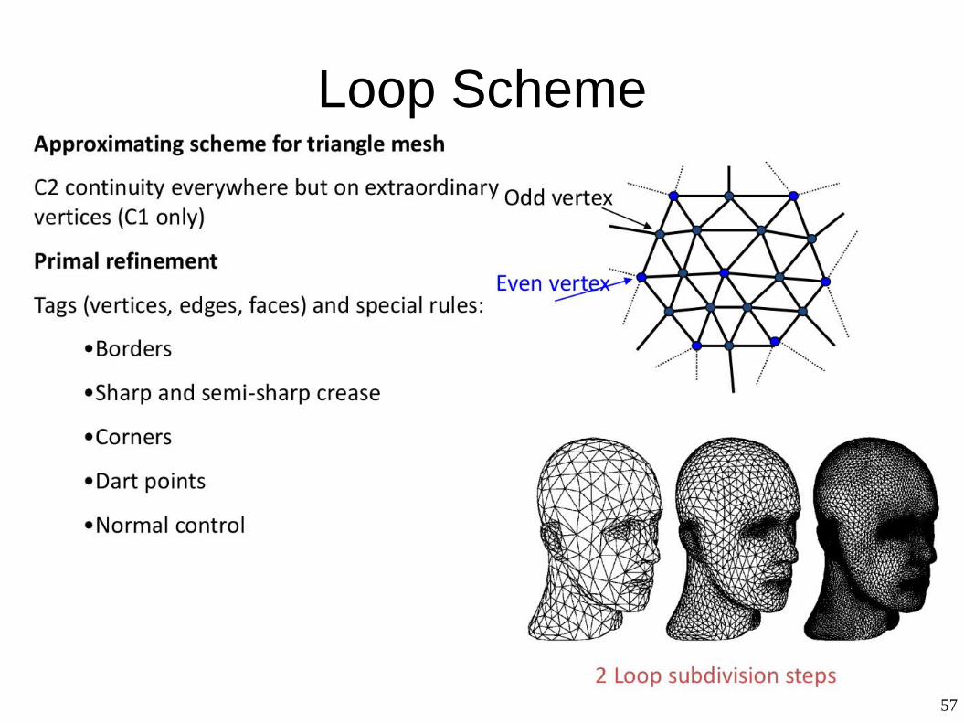
Loop Scheme
58
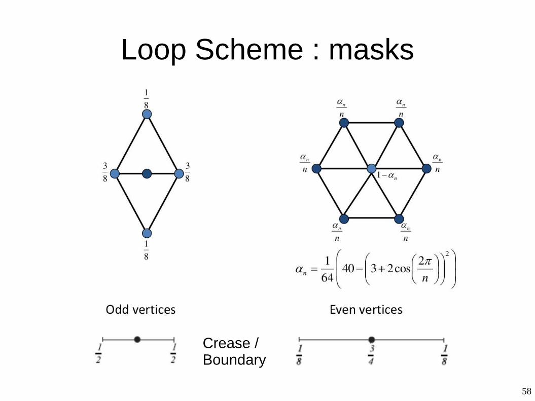
Loop Scheme : masks
Crease / Boundary
59
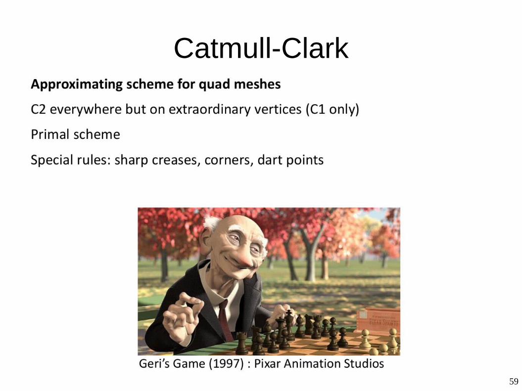
Catmull-Clark
60
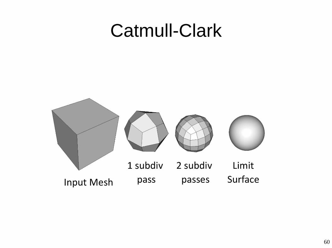
Catmull-Clark
61
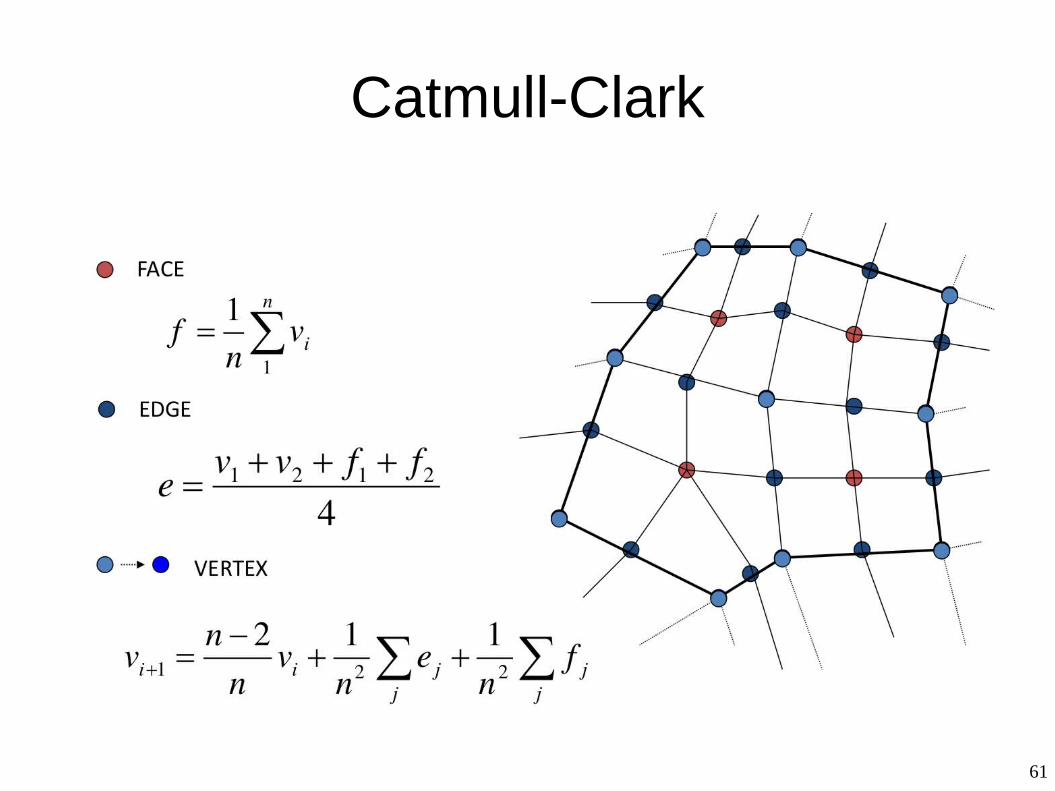
Catmull-Clark
62
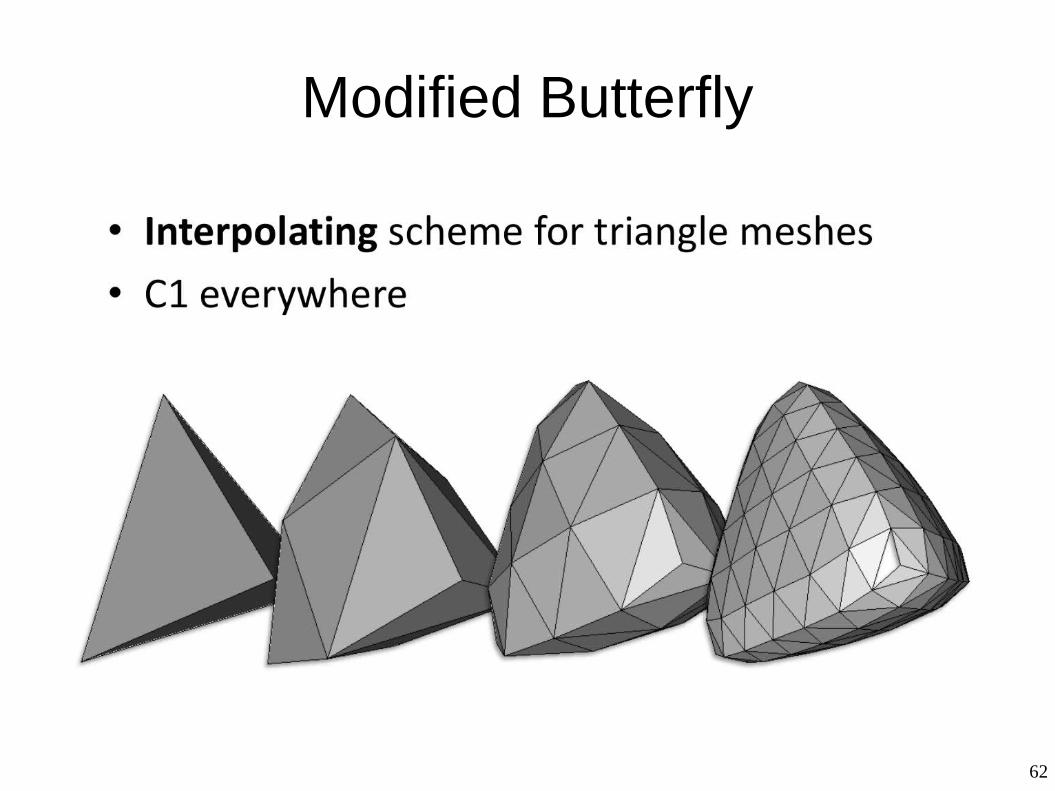
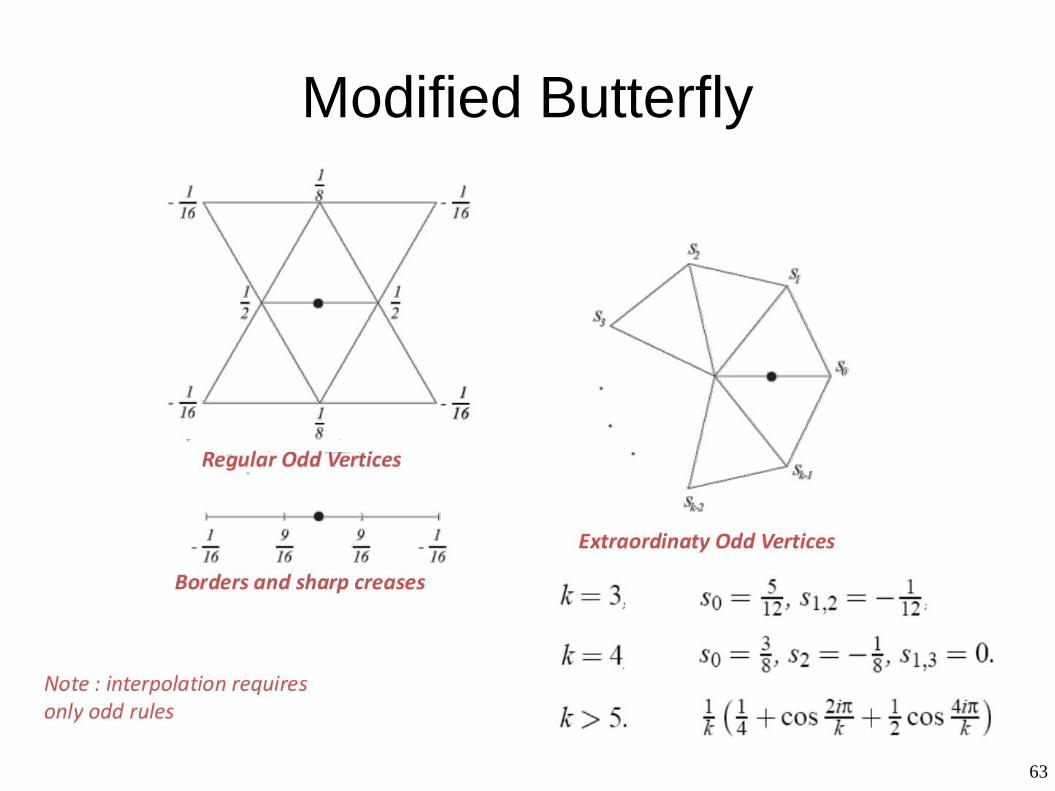
Modified Butterfly
63
Modified Butterfly
64
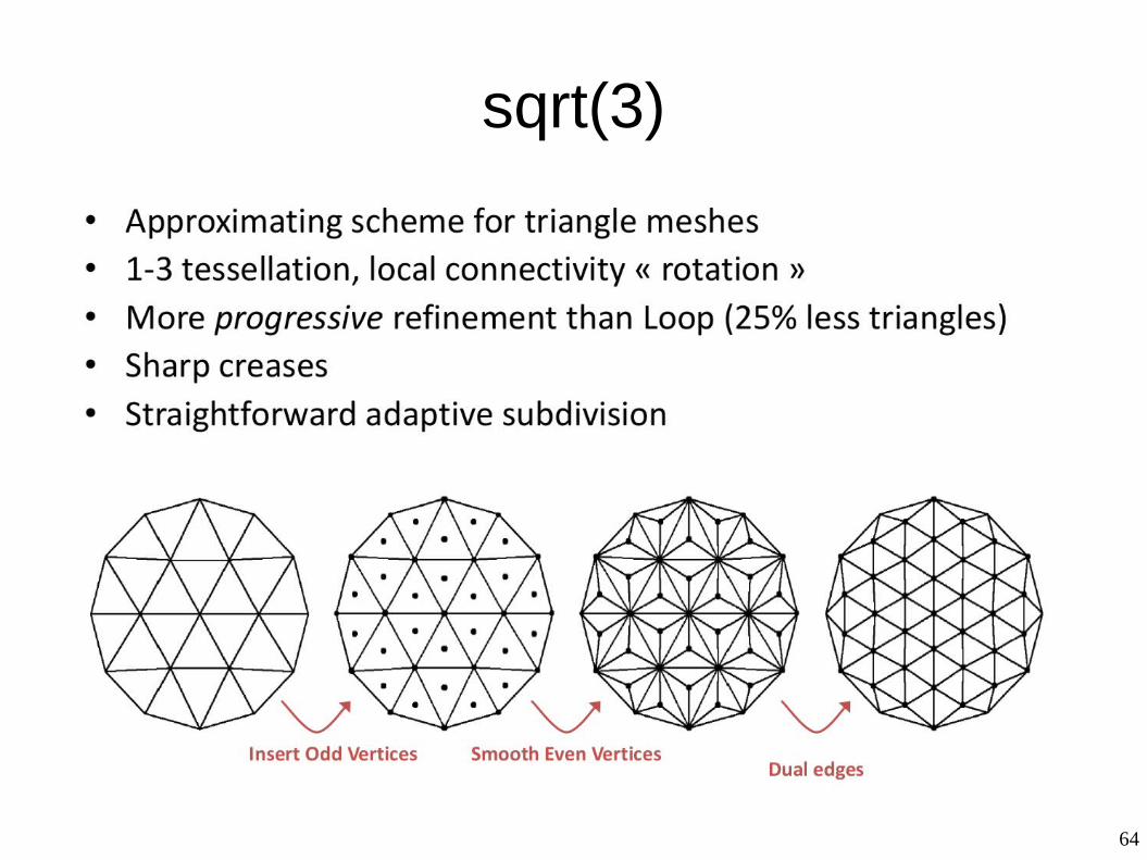
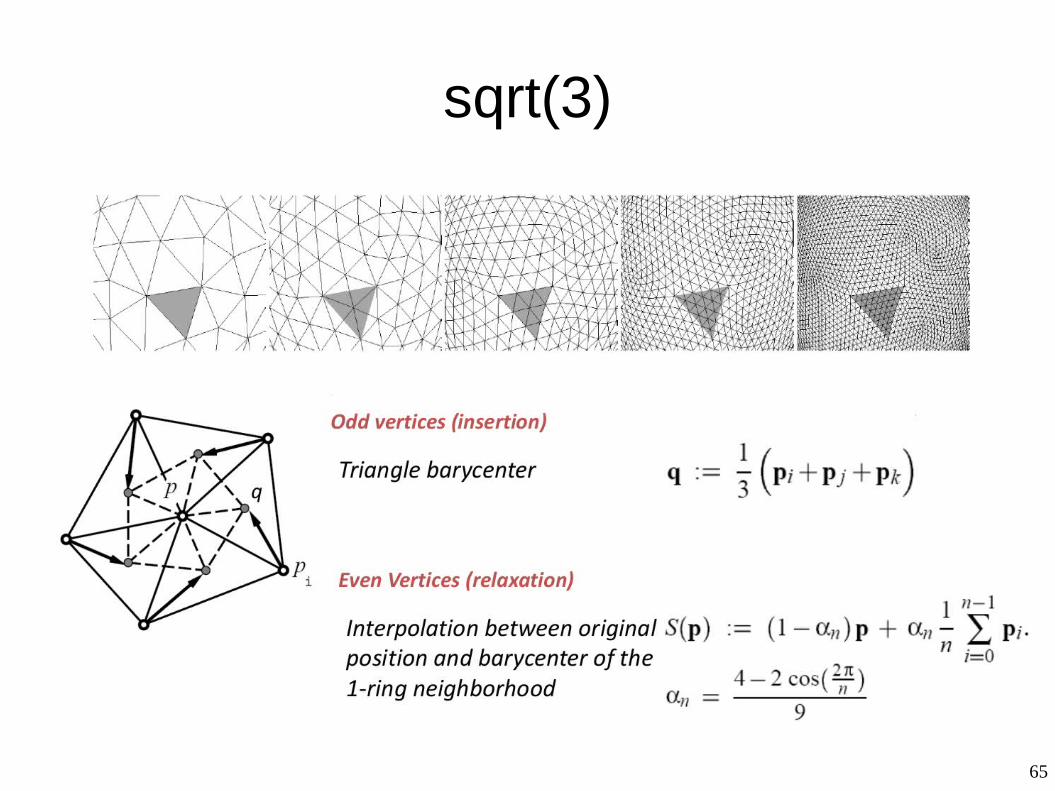
sqrt(3)
65
sqrt(3)
66
Subdivision matrix
67
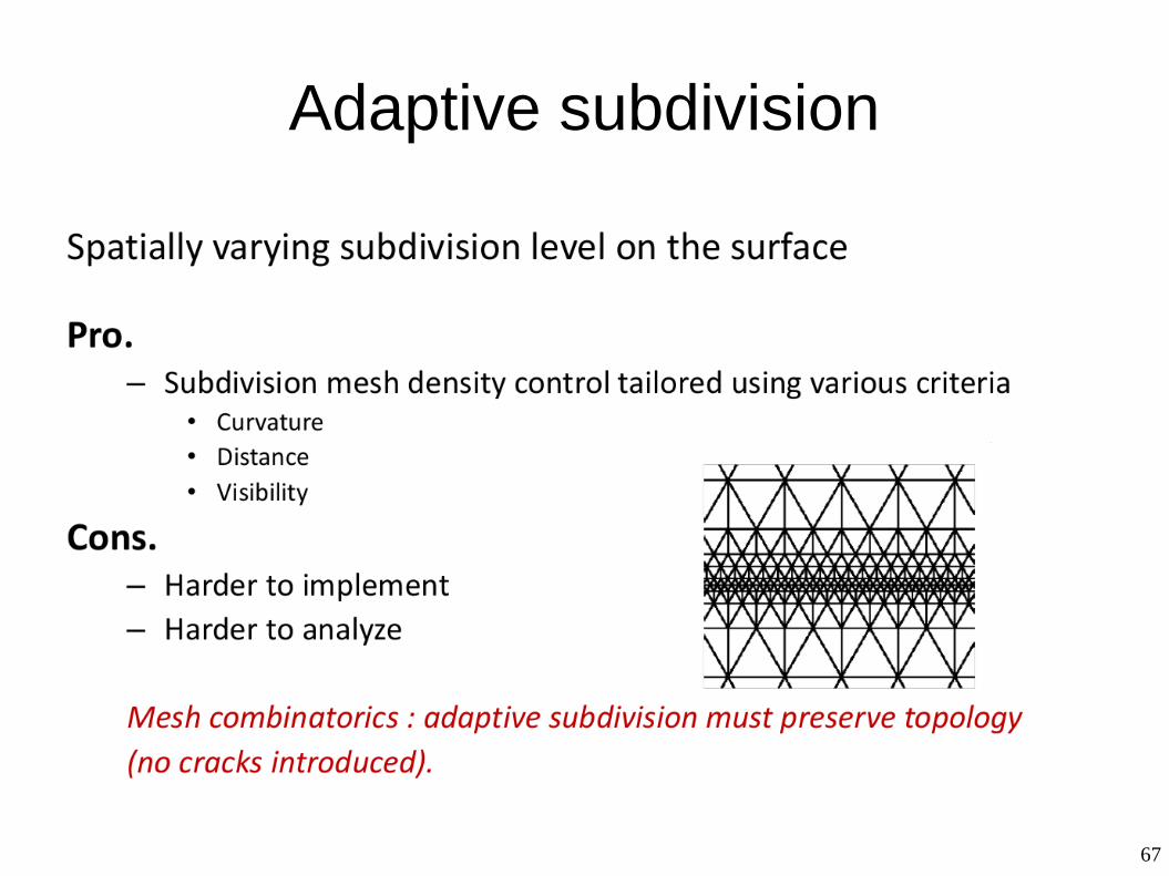
Adaptive subdivision
68
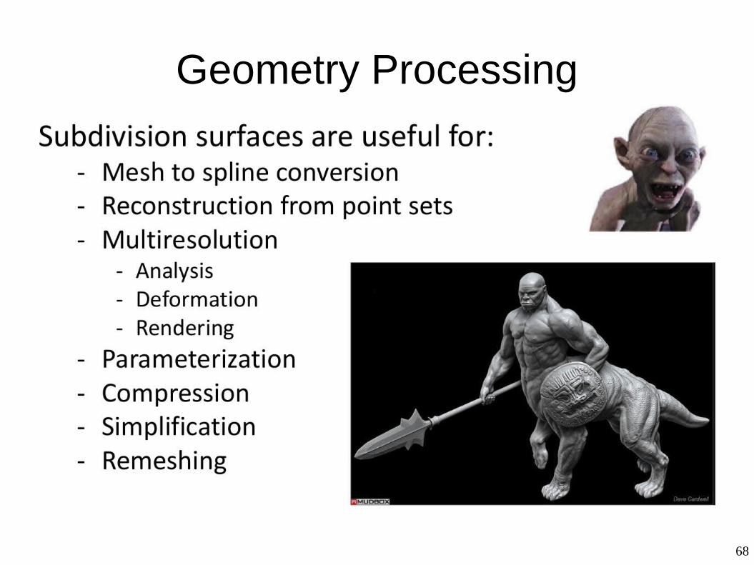
Geometry Processing
69
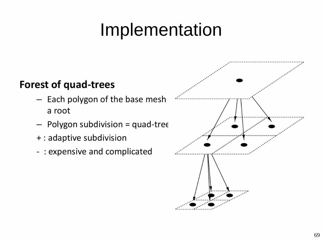
Implementation
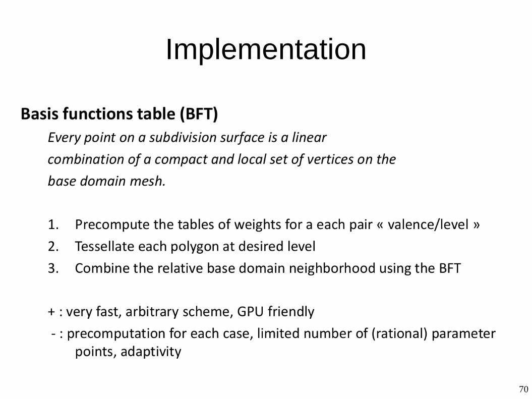
70
Implementation
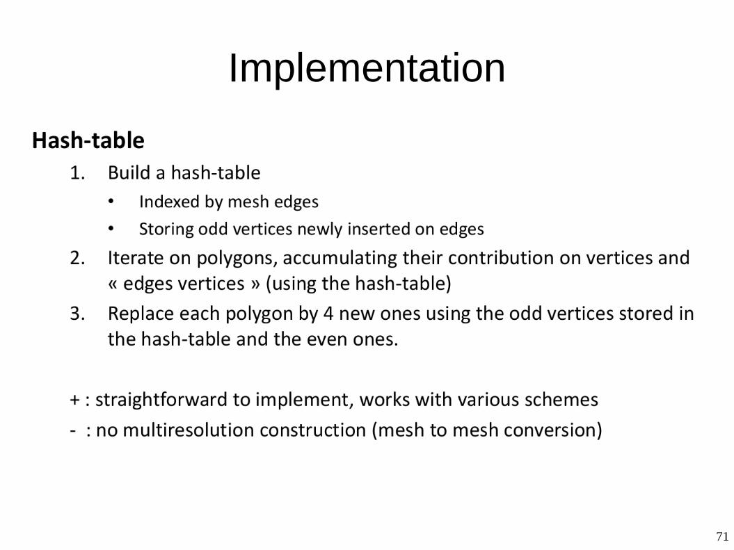
71
Implementation
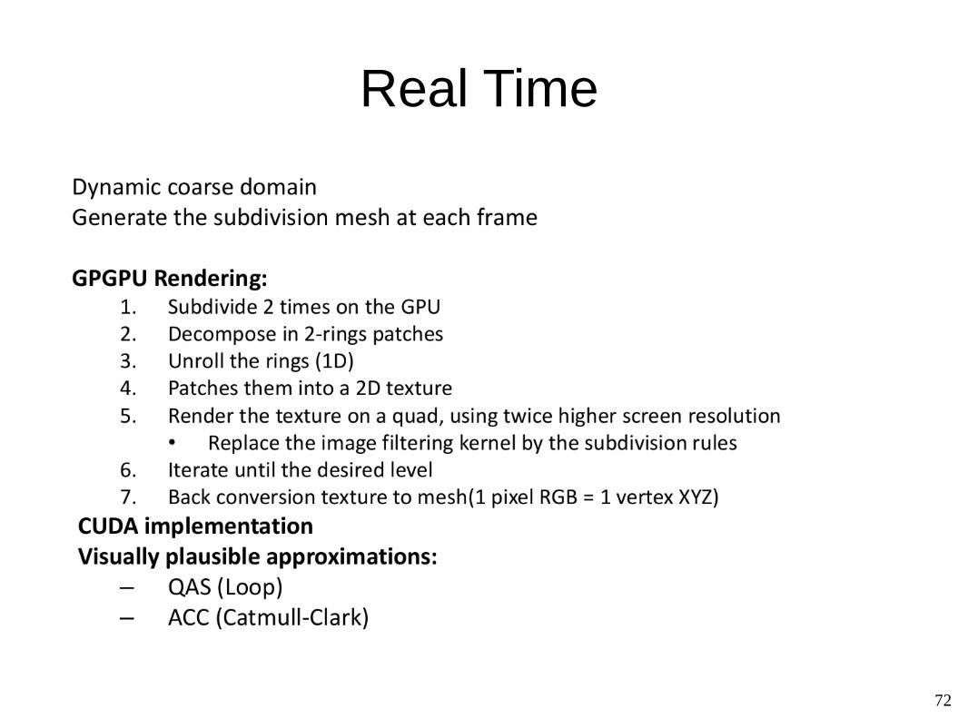
72
Real Time
73
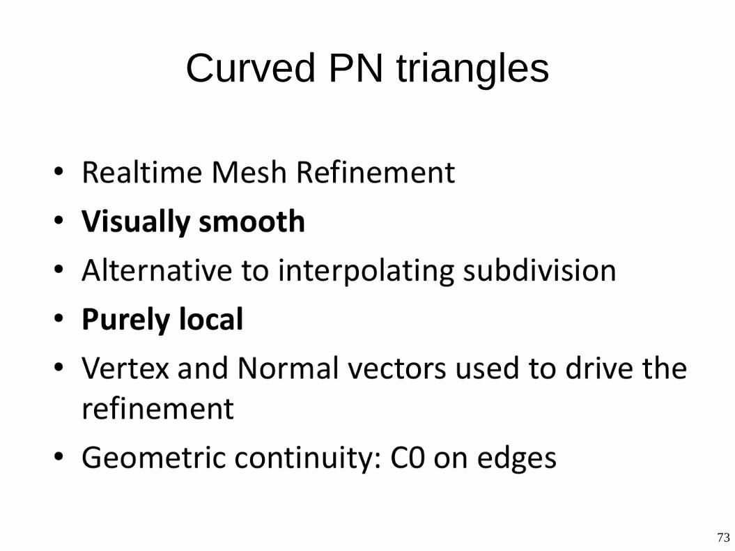
Curved PN triangles
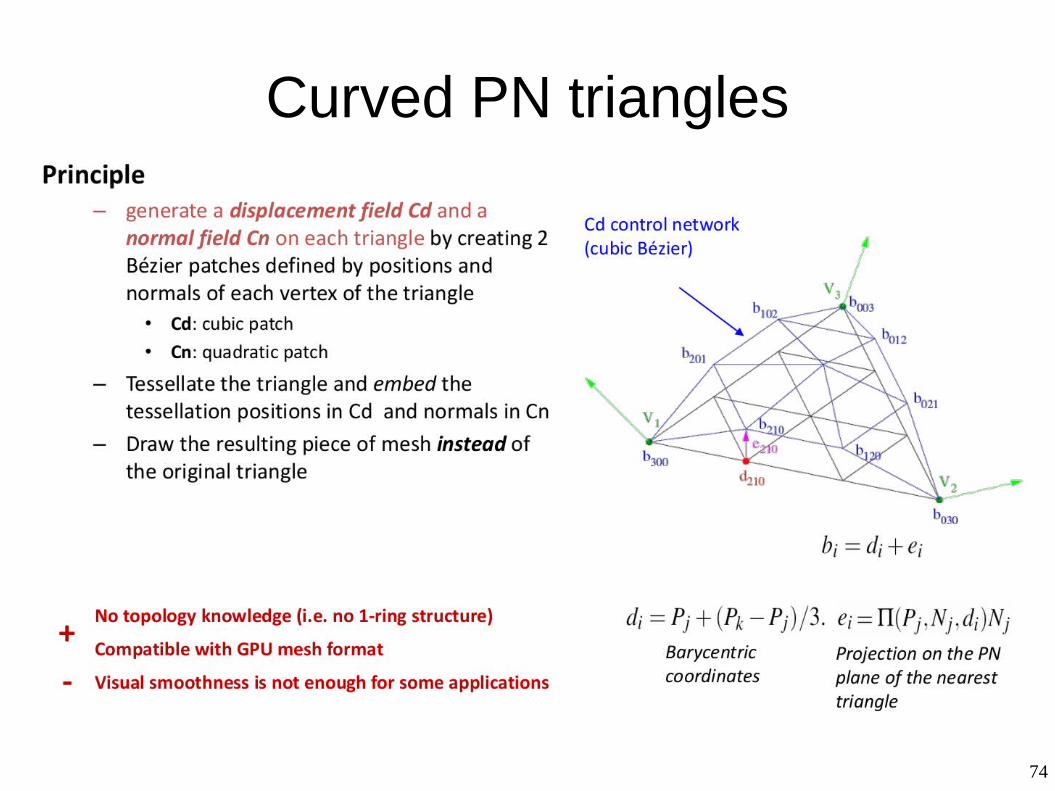
74
Curved PN triangles
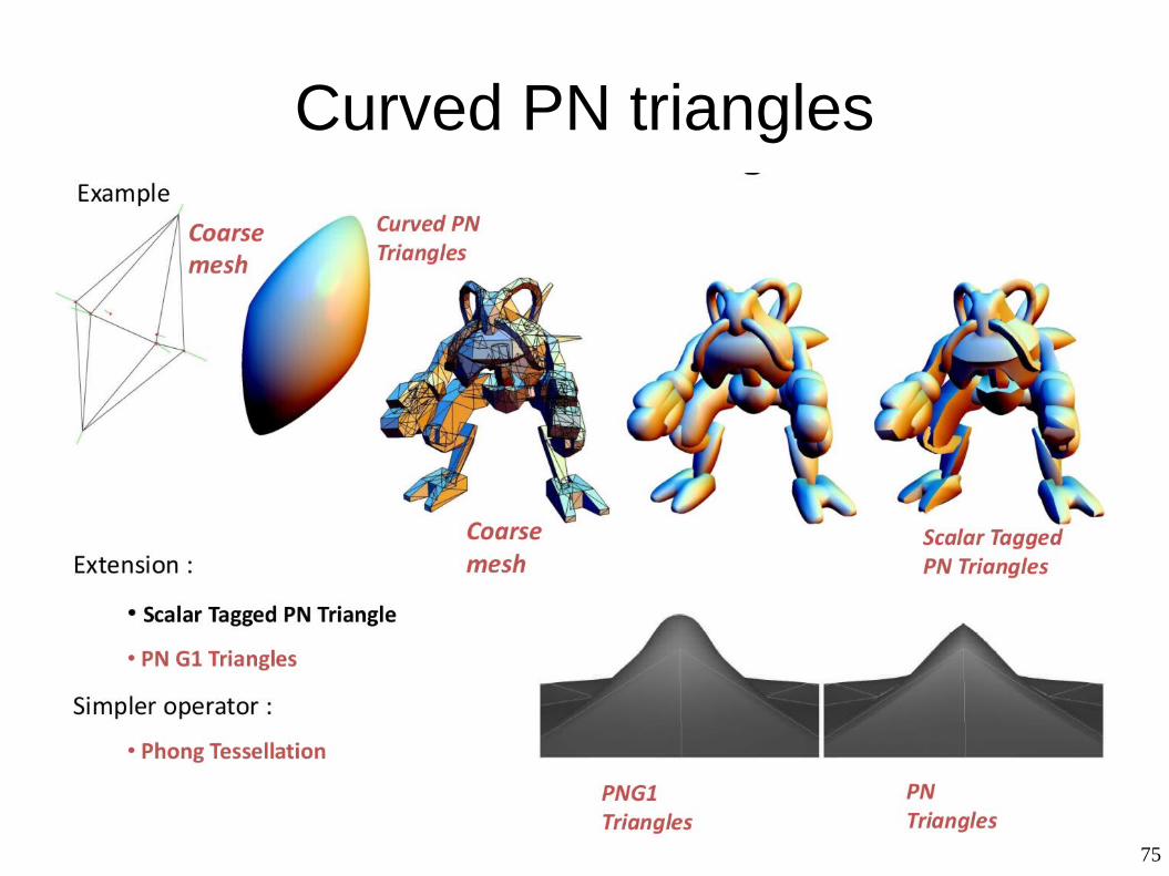
75
Curved PN triangles
76
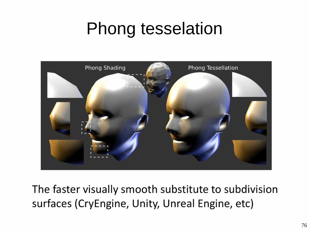
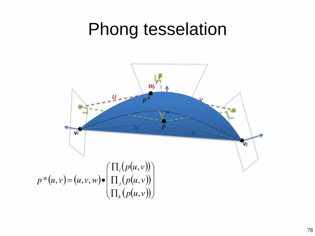
Phong tesselation
77
Phong tesselation
78
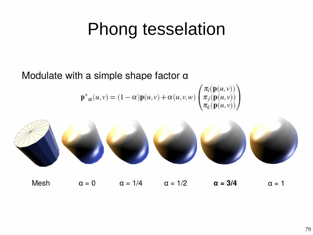
Phong tesselation
79
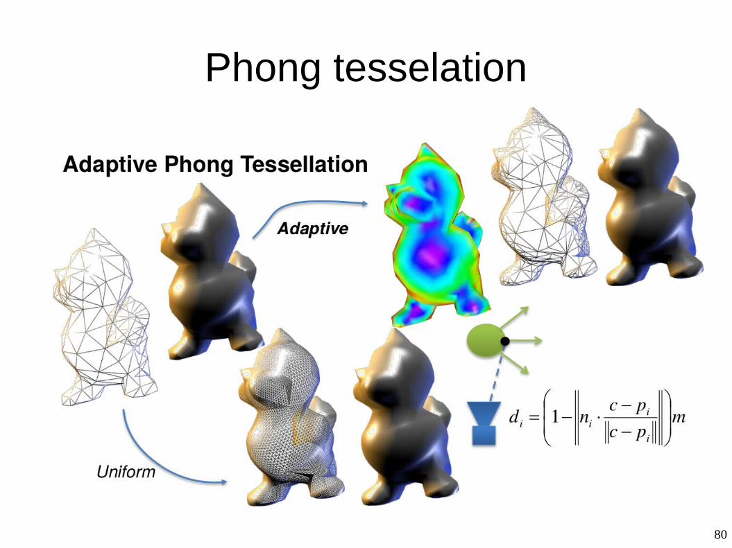
Phong tesselation
80
Phong tesselation
81
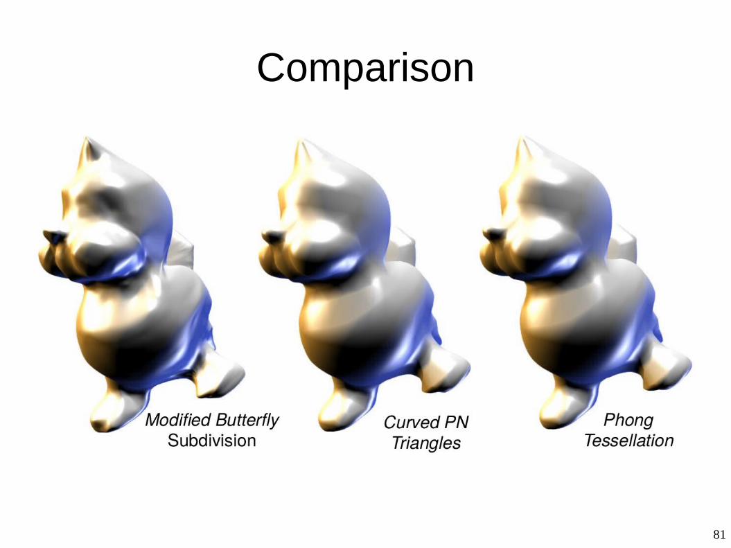
Comparison
82
Phong tesselation
83
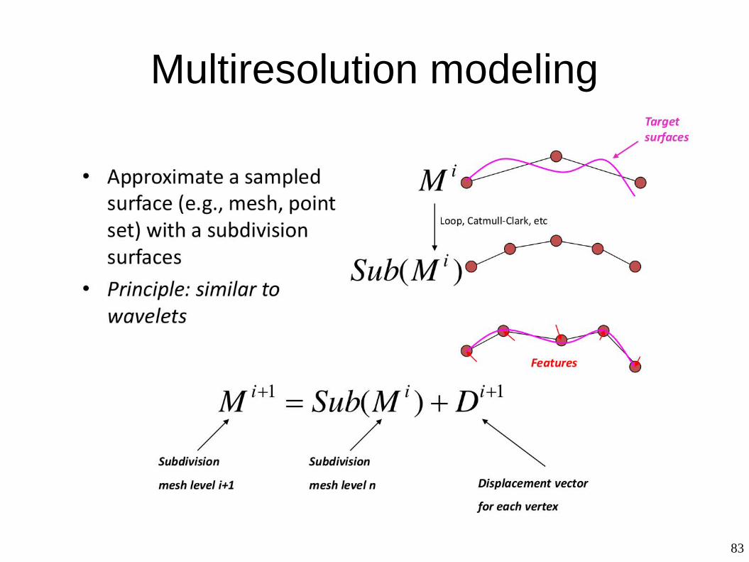
Multiresolution modeling
84
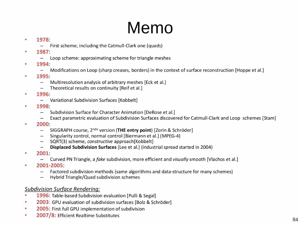
Memo
85
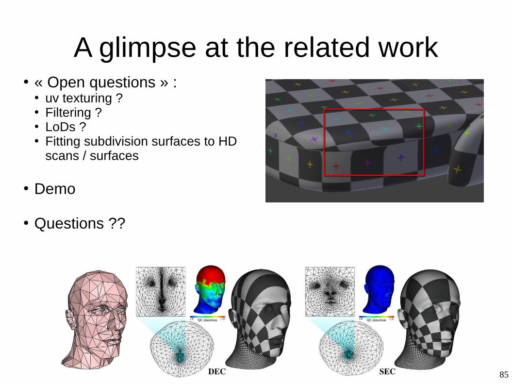
A glimpse at the related work● « Open questions » :
● uv texturing ?● Filtering ?● LoDs ?● Fitting subdivision surfaces to HD
scans / surfaces
● Demo
● Questions ??