Embed Size (px)
Citation preview
Dottorato di Ricerca in Matematica
Dipartimento di Matematica “G.Castelnuovo”
Grassmannians, Lie algebrasand quaternionic geometry
Andrea Gambioli
Universita degli studi di Roma “La Sapienza”
Facolta di Scienze Matematiche, Fisiche e Naturali

Dottorato di Ricerca in Matematica - XVII cicloSede Amministrativa:Universita degli studi di Roma “La Sapienza”
Relatore di tesi: Coordinatore del Dottorato:Prof. Simon Salamon Prof. Alberto Tesei
(Politecnico di Torino) (Universita “La Sapienza”di Roma)
Tesi presentata per il conseguimento del titolo di Dottore di Ricerca inMatematica nel mese di Dicembre 2005

Contents
Introduction III
Aknowledgements VI
1 Homogeneous spaces and Lie algebras 11.1 Homogeneous and Symmetric spaces . . . . . . . . . . . . . . 11.2 Adjoint orbits . . . . . . . . . . . . . . . . . . . . . . . . . . . 61.3 The consimilarity action . . . . . . . . . . . . . . . . . . . . . 91.4 Lie algebra cohomology . . . . . . . . . . . . . . . . . . . . . . 16
2 Geometry of Grassmannians 212.1 Bundles on Grassmannians . . . . . . . . . . . . . . . . . . . . 212.2 Sections obtained by projection . . . . . . . . . . . . . . . . . 232.3 The Twistor equation . . . . . . . . . . . . . . . . . . . . . . . 272.4 Invariant forms on Grassmannians . . . . . . . . . . . . . . . . 30
3 Functionals on G3(g) 363.1 The functional f . . . . . . . . . . . . . . . . . . . . . . . . . . 363.2 The functional g . . . . . . . . . . . . . . . . . . . . . . . . . 433.3 Hessians . . . . . . . . . . . . . . . . . . . . . . . . . . . . . . 463.4 Low dimensional examples . . . . . . . . . . . . . . . . . . . . 513.5 New critical manifolds for gradg . . . . . . . . . . . . . . . . 57
4 Quaterion-Kahler spaces 624.1 The Wolf Spaces . . . . . . . . . . . . . . . . . . . . . . . . . 624.2 The Twistor space . . . . . . . . . . . . . . . . . . . . . . . . 644.3 The Sp(1)Sp(n) structure . . . . . . . . . . . . . . . . . . . . 684.4 The quaternionic 4-form in 8 dimensions . . . . . . . . . . . . 73
5 Moment mappings and realizations 795.1 The moment mapping . . . . . . . . . . . . . . . . . . . . . . 795.2 Nilpotent orbits and Swann’s theory . . . . . . . . . . . . . . 82

5.3 A trajectory for so(4) . . . . . . . . . . . . . . . . . . . . . . . 875.4 Realizations in cohomogeneity 1: HPn . . . . . . . . . . . . . . 925.5 Realizations in cohomogeneity 1: G2(C
2n) and G4(Rn) . . . . . 99
6 Latent quaternionic geometry 1096.1 The Coincidence Theorem . . . . . . . . . . . . . . . . . . . . 1096.2 The two Twistor equations . . . . . . . . . . . . . . . . . . . . 1166.3 The interpretation of the functional g . . . . . . . . . . . . . . 1206.4 The case of su(3) . . . . . . . . . . . . . . . . . . . . . . . . . 1256.5 Still open questions . . . . . . . . . . . . . . . . . . . . . . . . 136
Bibliography 137
II

Introduction
Let G be a compact Lie group and g its Lie algebra.The main object ofstudy of this thesis is the Grassmannian
G3(g) = oriented 3-dimenisonal subspaces of g . (1)
We shall discuss both the theory for general G and special cases such asg = so(4) (which is not simple) and g = su(3).
We shall study the relationship between G3(g) and quaternionic geom-etry which ultimately derives from the QK moment mapping discussed inChapter 5, but we first study G3(g) without reference to Quaternion-Kahlermanifolds. Some sort of quaternionic structure is already evident in the de-scription of the tangent space of G3(g), even though the dimension of this isa multiple of 3, rather than 4. If V ∈ G3(g) then we can write g = V ⊕ V ⊥
and (using the metric on V )
TV G3(g) ∼= V ⊗ V ⊥ . (2)
Now V is the standard (and adjoint) representation of SO(3) which also ap-pears in quaternionic geometry as the space Im H generated by the imaginaryquaternions ı, j, k, or the corresponding almost complex structures I, J, K. Itis this identification of the “tautological” subspace V and Im H that underliesmany of the constructions in this thesis.
It is well known that much of the quaternionic geometry can ultimatelybe reduced to the representation theory of Sp(1) = SU(2). In particular, thecomplexified tangent space of a QK manifold M4n has the form
TxMC = Σ1 ⊗ C2n (3)
where we denote by Σk the irreducible complex representaion of SU(2) ofdimension k + 1. In appropriate circumstances the second factor C2n willitself be a representation of SU(2) and we shall be especially interested inan SU(2) equivariant inclusion
Σ1 ⊗ Σk−1 ⊂ Σ2 ⊗ Σk , (4)
which models inclusions
M Ψ G3(g) (5)
in Swann’s theory (developed mainly in [79] and [80]). In this last settingmoment mappings µ arising from the action of G are used in order to obtain
III

inclusions of type (5), identifying the image with the unstable manifoldsMu ofthe gradient flow of an invariant functional f . On the other hand, the quater-nionic structure of these last is reconstructed starting from the HyperKalerstructure of nilpotent orbits O in the complexified Lie algebra gC, and usingthen an appropriate action of H∗: in this way the various O appear to bethe bundles U fibring over the corresponding Mu. In this thesis the pointof view will be different, in the sense that the quaternionic structure will bedescribed using the map Ψ induced by the moment mappings and exploitingthe quaternionic structure inherent in the tangent space TV G3(g) in corre-spondence of the critical points for grad f , as in (4).
We give now an outline of the thesis chapter by chapter:
-Chapter 1 contains basic material about homogeneous and symmetricspaces (Section 1),Adjoint orbits (Section 2), together with the discussion ofthe consimilarity action (Section 3), which will be relevant for Section 4 inChapter 5; then cohomological properties of compact semisimple Lie goupsare discussed (Section 4), included the invariant 3-form which gives rise tothe functional f studied in Chapter 3.
-Chapter 2 describes bundles on Grassmann manifolds (Section 1), and in-troduces twistor-type differential operators existing on the tautological bun-dle (Sections 2, 3); these operators resemble the well-known twistor operatorsin QK geometry: in Chapter 6 a correspondence between them will be de-scribed; the deRham cohomology of G3(R
6) is calculated in Section 4,wherean explicit expression of an invariant 4-form of G3(R
n) for any n is supplied.
-Chapter 3 contains in Section 1 a description of the invariant functionalf on G3(g) coming from the standard 3 form of g, and introduces the Wolfspaces as its absolute maxima; an operator γ which represents an obstructionto the orthogonality of vector fields to G-orbits is introduced and used to dis-cuss the invariance of f in an alternative way. In Section 2, a new functionalg on G3(g) is introduced, and an expression for its gradient is given, in termsof a “generalized Casimir operator”; the invariance is discussed again usingthe operator γ. In Section 3 the Hessian of g is described at critical pointscorresponding to subalgebras, in therms of SU(2) representations; then wecompare it with the Hessian of f . In section 4 the theory discussed in theprevious sections is applied to some low-dimensional examples, determiningthe Hessians of f and g at grad f critical points; it is shown that not all crit-ical submanifolds for grad, g are critical for grad f , exhibiting examples andstating in Section 5 a criterion for individuating a family of such submani-folds.
-Chapter 4 introduces quaternionic geometry, describing firstly the basic
IV
facts of the classical theory, including the fundamental examples of the Wolfspaces (Section 1) together with their twistor space (Section 2); then thefirst bridge with the “Grassmannian interpretation” is built at an algebraiclevel, using SU(2) representation theory (Section 3); the quaternionic 4-formis introduced, and the previously discussed theory leads to an explicit de-scription of it in the setting of the 8-dimesnional case; this is related to thediscussion of the example corresponding to su(3) in Section 5 of Chapter 6.
-Chapter 5 introduces the QK moment mapping (Section 1); the rela-tionship with instantons,Nahm’s equations and nilpoten orbits theory andSwann’s theory are discussed: this latter contains the background regardingthe use of moment mappings to obtain the realizations of QK manifolds inG3(g); explicit examples of realizations in the case of some classical Wolfspaces are provided in Section 5, exploiting the knowledge of a trajectory forthe flow of grad f in the case of so(4) (Section 3); here the prorportionalityof grad f to grad g along this trajectory is proved: this will be used later inChaper 6.
-Chapter 6 consisnts of the main conclusions of the thesis: the Coinci-dence Theorem is stated and proved, providing a way of “translating” theaction of the quaternionic structure on the tangent space TxM of a QK man-ifold in the G3(g) setting; the operator γ introduced in Chapter 3 is involvedin this description of the quaternionic action.The correspondence betweenthe sections in the kernels of the two twistor operators (the “QK” and the“Grassmannian”) is described in Section 2; in Section 3 we consider againthe gradient of the functional g, studied in Chapter 2: it is proportional tograd f in several cases, and this fact seems significant in order to relate thequaternionic metric of the unstable manifold with that induced by the am-bient Grassmannian; finally the example of SU(3), which for some aspectsstands out of the general situation, is discussed in more detail in Section 4.
Notational conventions.
We will adopt the notation [V ] and [[V ]] = [V +V ] from [73] to denote the realvector space fixed by an invariant real structure in the complex representationV or V + V ; however we will sometimes omit the brackets for simplicity.
We will denote by exp the exponentiation of matrices and in the Lie alge-bra context, by Exp the exponentiation in the sense of Riemannian geometry.
Antisymmetric and symmetric product of tensors will be usually denotedby ∧ and ∨ respectively, but alternative notations will be adopted occasion-ally (for example in Section 4.3).
V

Aknowledgements
Before I proceed with the exposition, I wish to thank the people whoplayed an imprortant role on the way of writing this thesis.
First of all I am deeply grateful to my advisor Simon Salamon,withoutwhom the development of this project would not have been possible. I wantto thank him for his constant support, for sharing with me his far-seeing ideasand for the plenty of beautiful mathematics he has been teaching me duringthese years.
I was introduced to the study of Differential Geometry by MassimilianoPontecorvo, I wish to thank him for his precious advices and for his continuousinterest in my work.
Felt thanks go also to Andrew Swann for his valuable comments and forsending me so much material when I started to work on this project, and toYasuyuki Nagatomo for his relevant remarks and for useful discussions.
I wish to express my gratitude also to Stefano Marchiafava, Paolo Piccinniand Alessandro Silva in Rome,Elsa Abbena, Sergio Console,Anna Fino, SergioGarbiero and Antonio J. di Scala in Turin for their assistance and encour-agement.
Last, but not least, I wish to thank Diego Conti and Diego Matessi, whohave been stimulating student fellows for part of this journey.
RomaDecember 2005 A.G.
VI

Chapter 1
Homogeneous spaces and Liealgebras
In this Chapter, we shall cover a selection of topics relevant to the thesis. Thisincludes the less well-known action of SU(3) on itself induced from “consim-ilarity”.
1.1 Homogeneous and Symmetric spaces
We introduce here basic facts about G-actions and homogeneous spaces. Ref-erences are [81], [14], [25].
Let M be a differentiable manifold and G a compact Lie group.A C∞
map m : G×M →M such that
m(gh, x) = m(g,m(h, x)), m(e, x) = x (1.1)
for all g, h in G and x in M is called an action on the left of G on M and iscalled a G-space; analogous definitions give rise to actions on the right. Forsimplicity we will denote by g x the point m(g, x). Fixed a point x in M , wecall the orbit Gx of x under G the subset of M defined by
Gx := y ∈M |y = g x . (1.2)
Suppose that the orbit of a point x is the whole manifold M : then we will saythat G acts transitively on M , which is called a homogeneous G-space.Wedefine the isotropy subgroup (or stabilizer of p) Gp ⊂ G of an orbit Gp thesubgroup
Gp := g ∈ G |g , q = q (1.3)
for any point q ∈ Gp; in the transitive case all isotropy subgroups of areconjugate subgroups of G. The differential of the action of an element g ∈ Gp

1.1 Homogeneous and Symmetric spaces 2
at the point p determines a representation of Gp in GL(TpM) which is calledthe isotropy representation. In the case of transitive actions we can identifyM with the coset space of the group G:
M =G
Gp
(1.4)
for any point p ∈ G. In fact the space G/Gp can be topologized and equippedwith the correct differentiable strucure, so that a point p ∈ M can be iden-tified with a class g Gp for some g ∈ G. A map ψ : M → N between twomanifolds with a G-action is cvalled equivariant if it satisfies
ψ(g x) = gψ(x) (1.5)
for any g in G. If the action is not transitive, there exists an orbit withisotropy subgroup Gp such that gGpg
−1 ⊂ Gq for some g ∈ G and for anyother isotropy subgroup Gq; the corresponding orbit is of maximal dimensionand is called principal ; the union of pricipal orbits is an open dense subset ofM and the codimension of a principal orbit is called the cohomogeneity of theG action.Non-principal orbits Gq are called singular if dim Gq < dim Gp; ifdim Gq = dim Gp but Gp ⊂ Gq strictly, the orbit Gq is called exceprionaland is a discrete cover of the principal orbit Gp.
Examples.Consider the standard representation of SO(n) on Rn; as it pre-serves the standard euclidean norm,we have
GSn−1 ⊂ Sn−1 ; (1.6)
it can be shown that this action is transitive, and the subgroup Gp ⊂ SO(n)which stabilizes a unit vector (for example (0, · · · , 0, 1)) is isomorphic toSO(n− 1); in conclusion we can identify
Sn−1 ∼= SO(n)
SO(n− 1). (1.7)
This type of presentation is not unique:we can in fact analogously considerSU(n) acting on Cn with its standard hermitian structure; the sphere S2n−1
is again preserved, and the action can be again shown to be transitive onit; the stabilizer of a point turns out to be SU(n− 1) ⊂ SU(n), hence
S2n−1 ∼= SU(n)
SU(n− 1). (1.8)
Other important examples are projective spaces:CPn parametrizes the set ofcomplex lines C ⊂ Cn (which are real 2-planes preserved by the standard

1.1 Homogeneous and Symmetric spaces 3
complex structure J of Cn+1 = R2n+2); then the group U(n + 1) acts tran-sitively on such set, and one of the complex lines is fixed by the subgroupU(1) × U(n), so that
CPn ∼= U(n + 1)
U(1) × U(n). (1.9)
analogous considerations lead to the description of real and quaternionicprojective spaces:
RPn ∼= SO(n+ 1)
O(n), HPn ∼= Sp(n+ 1)
Sp(1)Sp(n). (1.10)
An important class of homogeneous G-spaces is that of symmetric spaces.References for this topic are [35] and [55].
Let (M, g) Riemannian manifold; consider a normal neighborood Np of apoint p ∈ M , where the Expp map is a local diffeomorphism with a neigh-bourhood of 0 in TpM ; we can define a map
dσp : TpM TpM (1.11)
acting as −I; this induces a local involutive diffeomorphism σp of the normalneighbourhood Np in itself called Cartan involution, sending a geodesic γ(t)through p to γ(−t); we have
Definition 1.1. A Riemannian manifold M for which the map σp is anisometry for every p ∈M is called a locally symmetric space.
Theorem 1.1. Let M be a Riemannian manifold; then the following condi-tions are equivalent:
i)M is locally symmetric;ii)∇R = 0 ,
where R is the Riemannian curvature tensor.
The symmetry is defined locally and in general it is not possible to extendit to a global isometry of the manifold M ; in this case M is defined a globallysymmetric space, or simply symmetric space. The following proposition relatesthe two notions:
Proposition 1.2. Let M be a complete locally symmetric space; if π1(M) = 0then M is globally symmetric.

1.1 Homogeneous and Symmetric spaces 4
Hence we can obtain globally symmetric spaces considering the universalcoverings of complete locally symmetric spaces. Symmetric spaces are homo-geneous, then if G is the full group of isometries for M we have a presentation
M = G/H (1.12)
where H is the stabilizer of a point p;σp induces an involutive automorphismof G, called Cartan involution:
sp(g) = σp g σ−1p , (1.13)
such that if Gσ denotes the subgroup fixed by sp and G0σ the connected
component of the identity, then
G0σ ⊂ H ⊂ Gσ ; (1.14)
at a Lie algebra level sp induces an automorphism of Lie algenras dsp witheigenvalues ±1, being involutive; therefore the decomposition
g = h + m (1.15)
corresponds to the identification of the + eigenspace with h and the − eigen-space with m ∼= TpM . A triple (g, h, ds) where h is a compact Lie subalgebraof the Lie algebra g and ds is an involutive Lie algebra automorphism suchthat h coincides with its + eigenspace is called an orthogonal Lie algebra; ifmoreover h ∩ z = 0,where z is the center of g, then the algebra is said effec-tive. For an orthogonal Lie algebra the following relations hold:
[h, h] ⊂ h, [h,m] ⊂ m, [m,m] ⊂ h ; (1.16)
exists a bijective correspondence between orthogonal Lie algebras and sym-metric spaces G/H with G simply connected and H connected,where N ∩His discrete if N is the maximal normal subgroup of G.
ExamplesAll examples discussed about homogeneous spaces (so Sn, CPn,RPn, HPn) are actually symmetric spaces.
Another example which will be particularly relevant for us is that of thereal oriented Grassmannians Gk(R
n): these represent the set of k-dimensionalsubspaces in Rn; as symmetric spaces they have a presentation
Gk(Rn) =
SO(n)
SO(k) × SO(n− k); (1.17)
the group SO(n) acts transitively on the set of orthonormal frames of Rn, buta k-plane V is identified by a k-tuple of orthonormal vectors, which can be

1.1 Homogeneous and Symmetric spaces 5
completed by an (n− k)-tuple in V ⊥; therefore SO(k) and SO(n− k) act onV ,V ⊥ respectively, and their tensor product coincides with the stabilizer ofthe point V .
Observation.The same symmetric space can have different presentations asa homogeneous space: not all of them give a decomposition (1.15) compatiblewith the involution, satisfying therefore (1.16); consider for insatnce the twopresentations of S2n−1 given in (1.7) and (1.8): the former is symmetric, thelatter is not.
A symmetric space M = G/K can be embedded as a totally geodesicsubmanifold of the Lie group G with the Riemannian metric induced by theKilling form by the map
g H gsg−1 (1.18)
called Cartan embedding, where gs is the image of g under the Cartan invo-lution s at a point p. Recall now from [17] that a Cartan subalgebra h whoseintersection with k is a Cartan subalgebra for k is called fundamental for thesymmetric decomposition, and its root system can be decomposed as:
∆ = Ik + Im + II (1.19)
where α belongs to Ik (or in Im) if α|hm = 0 and gα lies in kC (or in mC), whileα ∈ II if α|hm = 0.
We can use the roots of type Im to obtain minimal immersions of 2-spheres in any symmetric space G/K: consider α ∈ Im, then in gC the triplegα, g−α, [gα, g−α] spans an sl(2,C) subalgebra, containng an su(2) as thestable set for the appropriate real structure; the semisimple element [gα, g−α]intersects k in a 1-dimensional subalgebra u(1); therefore the correspondinghomogeneous space is
S2 =SU(2)
U(1). (1.20)
The immersion iα : SU(2) ⊂ G induces an equivariant immersion of sym-metric spaces
SU(2) iα
G
S2
φα
G/K
(1.21)
and the following proposition holds (see always [17]):
Proposition 1.3. Let G/K be a compact simply connected symmetric space;then if π2(G/K) is non-trivial, it is generated by the class [φα] for some α ∈Im.

1.2 Adjoint orbits 6
1.2 Adjoint orbits
We recall here some definitions and lemmas which will be useful in the se-quel: we recall that given the action of a compact group H of isometries on aRiemannian manifold M , we define a section Γ a smooth submanifold whichintersects transversally all the H-orbits; an H-action admitting a section iscalled polar, and if the section is flat it is called hyperpolar. Sections are al-ways totally geodesic submanifolds; in this sense the geodesic γ used for HPn
was a section. Fixed a point p ∈ M , we have the H-orbit through p, and thestabilizer Hp fixing p acts on TpM , preserving the subspace tangent to theorbit Tp (H · p), the isotropy representation, and its orthogonal complementνp (G · p), called slice representation; the following useful lemma holds:
Lemma 1.4. The cohomogenity of the H-action on M equals that of theHp-action on the slice representation.
Remark.We notice that in this language what we used to call the isotropyrepresentation of a homogeneous space M = G/K paradoxically coincideswith the slice representation.
References about hyperpolar actions on symmetric spaces are [36], [37], [56],[68] and [12]. From [68] we quote the following lemma, that gives a sufficientcriterion to individuate sections:
Lemma 1.5. If Γ is a compact, connected, flat, totally geodesic submanifoldof a Riemannian H-manifold M and Γ is orthogonal to some H-orbit at onepoint, then Γ meets all H- orbits orthogonally. If in addition the dimension ofΓ is equal to the cohomogeneity of the action on M , then Γ is a section andthe H action on M is hyperpolar.
Examining the proof that TpΓ ⊂ νp (with equality if p belongs to a prin-cipal orbit) and Γ can be obtained from Exp(TpΓ) for any p ∈ Γ. In con-sequence of this, if we pick a point p, we choose a vector y ∈ νp such thatγ(t) = Exp(ty) is a closed geodesic, then it is automathically a section, forcohomogeneity 1 actions.As we shall see, using sections is convenient to de-termine the behaviour of equivariant maps. In particular recall (see [14,ChapterIV,Theorem 3.1]) that the set of principal orbits in the orbit spaceM/G of a given compact G-manifold M is open, dense and connected, and inthe case of cohomogeneity 1 actions it corresponds to the whole M/G if it isan S1, or equivalently when the orbits are all principal; otherwise (and this isthe case we are most interested in) to the interior (0, 1) when M/G ∼= [0, 1].

1.2 Adjoint orbits 7
A well known action of a Lie group on itself is the Adjoint action; this isdefined in the followig way: if g, h ∈ G then
Adg · h := ghg−1 . (1.22)
Clearly the unit e is a fixed point for this action, and the differential inducedon TeG = g gives rise to the Adjoint representation, or in other words aninclusion G/Z ⊂ GL(g), where Z is the center of G. The principal orbit forthis action have the form
G
T n, (1.23)
where T n is a maximal torus for G, and they are called flag manifolds ; themotivation for this name relies on the fact that for SU(n) they represent themanifold of complete flags in Cn, that is of all sequences of complex vectorsubspaces
0 ⊂ V 1 ⊂ · · · ⊂ V n−1 ⊂ Cn (1.24)
where dimV k = k, with jumps of 1 dimension. Principal orbits form anopen dense subset in g; the following Theorem, due to Bott, describes therole played by maximal Abelian subalgenras:
Theorem 1.6. Each orbit for the Adjoint action of a centerless compactconnected Lie group G intersects a Cartan subalgebra t in a finite non-emptyset.
Example 1.1. Consider again the case of SU(n): from an elementary pointof view, Linear Algebra tells us that every skew-Hermitian matrix can be putin diagonal form ⎛⎜⎜⎜⎝
ıλk1 0 · · · 0
0. . . 0 0
0 0. . . 0
0 0 0 ıλkn
⎞⎟⎟⎟⎠ (1.25)
with λki∈ R and
∑i ki = 0 by conjugation with matrices in SU(n): in the
language developed above this corresponds to say that a maximal abeliansubalgebra t ⊂ su(n) is a global section for the Adjoint representation ofSU(n) on su(n), which therefore is a polar action and has cohomogeneityequal to its rank; as t inherits the flat metric from the ambient Euclideanspace g, the Adjoint action is hyperpolar. Exponentiating,we obtain the sametype of principal orbits for the action of SU(n) on itself, and the torus T n =exp t is again a section thanks to the surjectivity of exp:we shall see in section

1.2 Adjoint orbits 8
1.3 another type of action of SU(n) on itself with a rather different orbitstructure. Singular orbits are given by symmetric spaces of type
SU(n)
S(U(q1) × · · · × U(qr))(1.26)
with∑qi = n; these represent the manifolds of partial flags in Cn, analogous
to (1.24) but with dimensional jumps given by qi: in fact the principal or-bits (1.23) correspond to qi = 1 for all i. At the other extreme are complexGrassmannians, for which r = 2.Analogous situation holds for other classicalcompact semisimple Lie groups.
Another description of flag manifolds is obtained passing to the complex-ified group GC; consider the following type of subalgebras p ⊂ gC: p is calledBorel subalgebra if it is a maximal solvable subalgebra; it is called parabolicif it contains a Borel subalgebra. If we fix a Cartan decomposition
gC = tC ⊕∑
α
gα (1.27)
then an example of Borel subalgebra is given by
p = tC +∑α>0
gα (1.28)
and it can be shown that any other Borel subalgebra is conjugate to this one.Parabolic subalgebras are obtained by adding any negative simple root
spaces:
p = tC +∑α>0
gα +∑
β=
nααα∈I⊂∆+
g−β (1.29)
where I ⊂ ∆+ denotes any subset of the set of simple positive roots andnα ∈ Z+. Also in this case it can be shown that every parabolic subalgebra isconjugate to one of this type.Homogeneous spaces obtained by quotient as
GC
P(1.30)
where P = exp p can be shown to be compact, as they can be realized asorbits of the compact group:
GC
P∼= G
C(T k), (1.31)
where C(T k) is the centralizer of a k-torus with k ≤ rank G.

1.3 The consimilarity action 9
1.3 The consimilarity action
We are going now to consider the following group action c of GL(n,C) onitself, called consimilarity action:
c(A) · B := ABA−1 ; (1.32)
this action can be restricted to SU(n) ⊂ GL(n,C), so that SU(n) acts onitself, as in this case
ABA−1 = ABAt (1.33)
is in SU(n) if A, B are. This action is a special case of a family of actionsof a Lie group G on itself, described in [36]; these are constructed using anautomorphism σ of G and are called σ-actions.
First of all we prove
Lemma 1.7. The consimilarity action of SU(n) on itself is an isometricaction with respect to the Killing metric on SU(n).
Proof.Consider a curve B(t) ⊂ SU(3) such that B(0) = B0 and B(0) =w; then
d
dt(AB(t)At)|t=0 = AWAt ; (1.34)
therefore if w1, w2 ∈ TB0SU(n) then
〈w1, w2〉B0 = 〈B−10 w1, B
−10 w2〉e = Tr(B−1
0 w1B−10 w2) ; (1.35)
with B−10 wi ∈ su(n); analogously
〈Aw1At, Aw2A
t〉AB0At = 〈(AB0At)−1Aw1A
t, (AB0At)−1Aw2A
t〉e (1.36)
= 〈(At)−1B−10 A−1Aw1A
t, (At)−1B−10 A−1Aw2A
t〉e= Tr((At)−1B−1
0 w1At, (At)−1B−1
0 w2At)
= Tr(B−10 w1B
−10 w2) ;
the assertion follows.We can therefore use the machinery of smooth Riemannian actions to
describe the orbit structure of SU(n) as an SU(n)-space under consimilarityaction; from now on we concentrate on the case n = 3. Let us consider theorbit of the identity e = I under this action:
Proposition 1.8. The SU(3) orbit S of I under the consimilarity action isthe 5-dimensional symmetric space
SU(3)
SO(3). (1.37)

1.3 The consimilarity action 10
Proof.Consider the map
ξ :SU(3)
SO(3) S (1.38)
acting asASO(3) AAt ; (1.39)
it is well defined, as
AB(AB)t = ABBtAt = AAt (1.40)
if B ∈ SO(3); it is clearly surjective; it is also injective as if AAt = CCt then
C−1A = Ct(At)−1 =((C−1A)t
)−1(1.41)
so that C−1A ∈ SO(3), or in other words
ASO(3) = C SO(3) . (1.42)
From now on we shall write
SSU (3 ) :=SU(3)
SO(3)(1.43)
as an abbreviation.
Observation.Consider the totally geodesic immersion
ζ : ASO(3) AσA−1 (1.44)
as seen in (1.18), where the involution σ is given by
σ(A) = A ; (1.45)
then we have:ζ = σ ξ . (1.46)
We are intersted in calculating the cohomogeneity of this action and thegeneric orbit type, and in determining if possible the singular orbits. Theanswer to these questions is given in
1.3 The consimilarity action 11
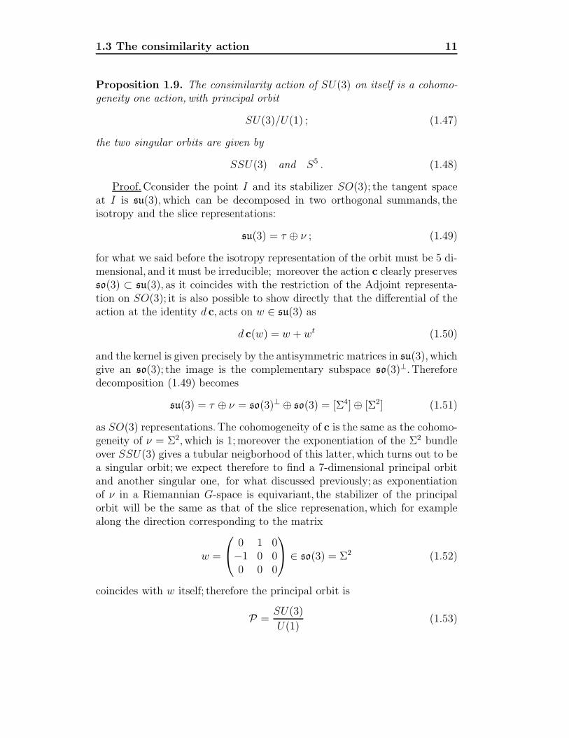
Proposition 1.9. The consimilarity action of SU(3) on itself is a cohomo-geneity one action, with principal orbit
SU(3)/U(1) ; (1.47)
the two singular orbits are given by
SSU(3) and S5 . (1.48)
Proof.Cconsider the point I and its stabilizer SO(3); the tangent spaceat I is su(3), which can be decomposed in two orthogonal summands, theisotropy and the slice representations:
su(3) = τ ⊕ ν ; (1.49)
for what we said before the isotropy representation of the orbit must be 5 di-mensional, and it must be irreducible; moreover the action c clearly preservesso(3) ⊂ su(3), as it coincides with the restriction of the Adjoint representa-tion on SO(3); it is also possible to show directly that the differential of theaction at the identity d c, acts on w ∈ su(3) as
d c(w) = w + wt (1.50)
and the kernel is given precisely by the antisymmetric matrices in su(3), whichgive an so(3); the image is the complementary subspace so(3)⊥. Thereforedecomposition (1.49) becomes
su(3) = τ ⊕ ν = so(3)⊥ ⊕ so(3) = [Σ4] ⊕ [Σ2] (1.51)
as SO(3) representations. The cohomogeneity of c is the same as the cohomo-geneity of ν = Σ2, which is 1;moreover the exponentiation of the Σ2 bundleover SSU(3) gives a tubular neigborhood of this latter, which turns out to bea singular orbit; we expect therefore to find a 7-dimensional principal orbitand another singular one, for what discussed previously; as exponentiationof ν in a Riemannian G-space is equivariant, the stabilizer of the principalorbit will be the same as that of the slice represenation,which for examplealong the direction corresponding to the matrix
w =
⎛⎝ 0 1 0−1 0 00 0 0
⎞⎠ ∈ so(3) = Σ2 (1.52)
coincides with w itself; therefore the principal orbit is
P =SU(3)
U(1)(1.53)

1.3 The consimilarity action 12
with U(1) = exp(tu). The generic stabilizer U(1) has to be contained in boththe singular stabilizers, and in fact U(1) ⊂ SO(3); we are now looking for thesecond singular orbit, and to do that we exponentiate w in order to get aclosed geodesic, which will intersect orthogonally all the orbits by (1.5):
B(t) = exp(tw) =
⎛⎝ cos t sin t 0− sin t cos t 0
0 0 1
⎞⎠ . (1.54)
Set
Bs = B(π/4) =
⎛⎝ 0 1 0−1 0 00 0 1
⎞⎠ (1.55)
and let us consider the differential d c when acting at Bs: if w ∈ su(3) then
d c(w) = wBs +Bswt ; (1.56)
then the kernel of d c consists of the span of the elements⎛⎝ 0 1 0−1 0 00 0 0
⎞⎠ ,
⎛⎝0 ı 0ı 0 00 0 0
⎞⎠ ,
⎛⎝ı 0 00 −ı 00 0 0
⎞⎠ , (1.57)
which is the subalgebra su(2) ⊂ su(3) corresponding to the maximal root.Therefore the corrsponding orbit has the form
SU(3)
SU(2)= S5 (1.58)
in a non-symmetric presentation.This can be expressed alternatively by saying that each element A ∈
SU(3) is consimilar to B(t) for some t.We have therefore the following doublefibration associated to this orbit structure, as SU(2) ⊃ U(1) ⊂ SO(3):
SU(3)/U(1)π2
π1
SSU(3) S5
, (1.59)
where the projections π1 and π2 are obtained in the following way: given apoint p in a principal orbit SU(3)/U(1) exists a unique normal vector u, as itis a hypersurface in SU(3); therefore exists a unique geodesic γ which passesthrough p and is tangent to u;moreover γ is a section and can be obtained

1.3 The consimilarity action 13
from Bs through the consimilarity action.As γ must inersect the singularorbits, if we follow it in the two directions, we will define π1(p) as the firstintesection γ ∩ SSU(3) and π2(p) as the first intersection γ ∩ S5 .
Consider again the singular orbit SSU(3): it is a non-inner symmetricspace, and the symmetric decomposition of the Lie algebra su(3) is given by
su(3) = k + m = so(3) ⊕ [Σ4] ; (1.60)
let σ denote the induced group involution; then a σ-stable Cartan subalgebrat is given by the span of the elements
w =
⎛⎝ 0 1 0−1 0 00 0 0
⎞⎠ , w =
⎛⎝ı 0 00 ı 00 0 −2ı
⎞⎠ ; (1.61)
we notice that if t′ denotes the Cartan subalgebra generated by diagonalmatrices, then
t′ = BstB−1s ; (1.62)
with respect to (1.60), we have the decomposition
t = tk + tm (1.63)
which is expressed in terms of matrices by (1.61). Therefore if we considerthe usual roots ∆ α′ in t′∗
C, then
α = α′ AdB−1s
; (1.64)
moreover we notice that t∩ so(3) is spanned by w, which is obviously a max-imal abelian subalgebra for so(3). Consider now in particular the maximalroot α′
0 with respect to t′, which is the dual to⎛⎝0 1 00 0 00 0 0
⎞⎠ . (1.65)
It is known that π2(SSU(3)) = Z2 (see [17, Page 38]); we want to find a rootα ∈ Im in order to identifiy the generator S2 of π2; consider the restriction ofthe map ξ to the subgroup SU(2) corresponding to the long root α′
0: recallProposition 1.3 and diagram (1.21); then we have
Proposition 1.10. The map ξ defined in (1.38) coincides with φα′0
and itsimage is the generator of π2(SSU(3)).

1.3 The consimilarity action 14
Proof. In view of (1.65) and (1.61), we have that α|tm = 0 only for α′ =α′
0, so Ik + Im = α′0;moreover the corresponding root space is given by
gα′0
= t
⎛⎝ı 0 00 −ı 00 0 0
⎞⎠ ∈ m ; (1.66)
therefore Im = α0 and the SU(2)/U(1) corresponding to the highest rootgenerates π2(SSU(2)). In particular the semisimple element of su(2) corre-sponds to w, hence the thesis.
Going back now to the consimilarity action, let us consider the normalbundles ν1 and ν2 respectively at I and atBs: we are interested in determiningthe intersections
exp ν1 ∩ S5 and exp ν2 ∩ SSU(3) , (1.67)
or in other words the “limit points” of the geodesics emanating from a pointin one of the singular orbits when they meet the other the first time.
Proposition 1.11. The intersection exp ν2 ∩ SSU(3) is the S2 generatingπ2(SSU(3)).
Proof.The left multiplications on a Lie group are isometries with respectto the metric induced by the Killing form by definition, therefore they respectexponentiation:
exp ν2 = BsB−1s exp ν2 (1.68)
= Bs exp(B−1s ν2)
= BsExp (su(2))
= BsSU(2) = SU(2) ;
hence we have to determine SU(2) ∩ SSU(3);moreover as exp is equivari-ant, then the intersection is also given by exp(S2
π/4), whose image is a ho-
mogeneous manifold of the form SU(2)/K with K ⊃ U(1) where u(1) =tw, because of equivariance; but clearly we have
S2 = ξ(SU(2)) ⊂ SU(2) ∩ SSU(3) (1.69)
as in fact ξ(SU(2)) ⊂ SU(2); hence it must be K = U(1) and the conclusionfollows.
This can be interpreted in terms of the double fibration (1.59) by sayingthat
π1(π−12 Bs) = S2 . (1.70)
Analogous considerations lead to the following

1.3 The consimilarity action 15
Proposition 1.12. We have
exp ν1 ∩ S5 = S2 = SO(3)/U(1) = ABsAt |A ∈ SO(3) , (1.71)
with u(1) = tw .
Again in terms of (1.59)π2(π
−11 I) = S2 . (1.72)
We want now to discuss a link with the Adjoint action:we can define amap Φ : SU(3) −→ SU(3) acting as
Π(A) = AA ; (1.73)
first of all we observe that the map is equivariant with respect to the con-similarity action on the left and the AdSU(3) action on the right:
Φ(BABt) = BABt((BABt) = BAB−1 , (1.74)
therefore orbits are sent to orbits; in particular it is immediate to show that
Φ(SSU(3)) = I and Φ(S5) = CP2 (1.75)
and in fact
Φ(B(t)) = B(t)2 =
⎛⎝cos2 t− sin2 t 2 cos t sin t 0−2 cos t sin t cos2 t− sin2 t 0
0 0 1
⎞⎠ (1.76)
=
⎛⎝ cos 2t sin 2t 0− sin 2t cos 2t 0
0 0 1
⎞⎠ =: B(t) . (1.77)
We introduce now the AdSU(3)-invariant subspace H ⊂ SU(3) defined as
H = A ∈ SU(3) | Im Tr(A) = 0 ; (1.78)
clearly Φ(SU(3)) ⊂ H as
Tr(AA) = Tr(AA) = Tr(AA) , (1.79)
but moreover we have:
Lemma 1.13. The subset H ⊂ SU(3) is a connected and algebraic set, smootheverywhere excepted at I;moreover
Φ(SU(3)) = H . (1.80)

1.4 Lie algebra cohomology 16
Proof.We can characterize the elements of H as those which can be di-agonalized in the form
D(θ) =
⎛⎝eıθ 0 00 e−ıθ 00 0 1
⎞⎠ (1.81)
proving that it is arc-connected; this fact can be interpreted by saying thatD(θ) is the intersection T 2 ∩ H where T 2 is the diagonal maxima torus;therefore the AdSU(3) action restricted to H is a cohomogeneity 1 action. thecondition Tr(A) = Tr(A) can be put in an algebraic form considering thecharacteristic polynomial of a generic diagonalized element in SU(3):
T (λ) = −λ3 + (eıθ + e−ıφ + eı(φ−θ))λ2 + (e−ıθ + eıφ + eı(−φ+θ))λ+ 1 (1.82)
so that H is the zero locus of the function
P (a11, · · · a33) = a11 + a22 + a33 − a11a22 − a22a33 − a22a33 ; (1.83)
the gradient of this last is given in terms of θ, φ by
gradP (φ, θ) = (cos θ − cos (θ − φ),− cosφ+ cos(θ − φ)) (1.84)
which is zero if and only if θ ∈ 0, 2/3π,−2/3π and φ ∈ 0,−2/3π, 2/3πrespectively, or in other words at the center Z(SU(3)) = (1, ζ, ζ2) with ζ3 =1, and Z(SU(3)) ∩H = I. We finally prove the surjectivity of Φ: for this itwould be sufficient proving that
B(t) = C D(θ(t))C−1 (1.85)
for some C ∈ SU(3); but the eigenvalues of B(t) are easily seen to be1, 2t,−2t, therefore we are done putting θ(t) = 2t.
1.4 Lie algebra cohomology
First recall that the Lie algebra g of G corresponds to vector fields whichare invariant under left translations; in the same way g∗ corresponds to thespace of left invariant differential forms AL(G). Exterior differentiation dis compatible with any diffeomorphism φ : G → G in the sense that ifα ∈ AL(G)
φ∗(dα) = dφ∗α , (1.86)
and in particular this is true for left translations; so
dAL(G) ⊂ AL(G) , (1.87)

1.4 Lie algebra cohomology 17
or in other words the space AL(G) is stable under d.We will denote by dg
the restriction of d to AL(G) ∼= g∗, so that (∧
g∗, dg ) is a differential graded
algebra; ifXi, i = 1...k+1 are left invariant vector fields and if α ∈ ∧kg∗, then
dgα behaves in the following way:
dgα(X1, ..., Xk+1) =∑i<j
(−1)i+jα([Xp , Xq], X1, .., Xi, .., Xj, .., Xk+1) ;
(1.88)it is clear that (dg )2 = 0 , so we can form the cohomology groups
Hp(g) = HpL(G) . (1.89)
Denoting by θ the representation induced on g∗ by the adjoint repre-sentation,we can extend it to a representation θ∧ of g on
∧g∗; the subscript
θ = 0 will denote the subspace killed by θ∧, a.k.a. the space of biinvariant, orsimply invariant, forms; in other words
(∧
g∗) θ=0 := α ∈∧
g∗ | θ∧(α) = 0 . (1.90)
In case that G is connected, thanks to the surjectivity of the exp map ,thespace (
∧g∗) θ=0 coincides with the space (
∧g∗)I of forms fixed by the exten-
sion of the Ad representation of G on g. The space (∧
g∗) θ=0 is again stableunder d, but there is more; in fact
d((∧
g∗) θ=0
)= 0 . (1.91)
This can be shown in the following way: if ν denotes the inversion map ofg, so that ν(a) = a−1, then
ν∗α = (−1)pα , (1.92)
for any invariant form α of degree p ; then
(−1)p+1dα = ν∗dα = dν∗α = (−1)pdα , (1.93)
so dα must be 0.Thanks to this fact the inclusion of AI(G) in AL(G) inducesa homomorpism of algebras
(∧
g∗) θ=0∼= AI(G) HL(G) . (1.94)
The consequence is that under the hypoteses of the compactness andconnectedness of G we can reduce the problem of computing the cohomologyof G to that of computing the cohomology of g and, better, to the knowledgeof (∧
g∗) θ=0, as the following proposition states:

1.4 Lie algebra cohomology 18
Proposition 1.14. If the Lie group G is compact and connected, then all themaps in the following commutative diagram are isomorphisms of algebras:
AI(G)
∼=
HL(G)
∼=
H(G)
(∧
g∗) θ=0 H(g)
. (1.95)
Identifying (∧
g∗) θ=0 is not in general an obvious task, excepted in somecases: for example when G is abelian.
Example 1.2. If G is abelian then it must be an n-dimensional torus; in thiscase the adjoint representation θ is trivial, so that
(∧
g∗) θ=0 =∧
g∗ ; (1.96)
so the Betti numbers are just the dimensions of the various∧p g∗ for p = 0...n:
bp = dim Hp(G) = dim
p∧g∗ =
(n
p
)=
n!
p!(n− p)!; (1.97)
the Poincare polynomial is equal to (1 + t)n.We observe that thanks to theinclusion (
∧g∗) θ=0 ⊂
∧g∗ for any other compact connected Lie group G we
will have PG(t) ≤ (1 + t)n.
In general however it is possible to say something about the low Bettinumbers; we start defining a canonical linear map
ρ : (∨2 g∗) θ=0
(∧3 g∗) θ=0 (1.98)
in the following way: let Ξ ∈ (∨2
g∗) θ=0, then ρ(Ξ) = Φ is defined as
Φ(x, y, z) = Ξ([x , y], z) ; (1.99)
the invariance of Ξ implies that Φ is skew-symmetric, and the Jacobi identitythat it is invariant. We denote with f the image of the Killing form 〈 , 〉through ρ.
Proposition 1.15. Let g be a Lie algebra such that H1(g) = H2(g) = 0; thenρ is an isomorphism.
Thanks to this we can deduce the following facts:

1.4 Lie algebra cohomology 19
Proposition 1.16. Let g = g1⊕· · ·⊕gm be the decomposition of a semisimpleLie algebra in terms of simple ideals; then:
i)b1 = b2 = 0;
ii)b3 ≥ m;
iii)if the ground field Γ = C or if Γ = R
and the Killing form is negative definite, then b3 = m .
Proof. It is sufficent to consider the case m = 1.For i we just need toobserve that the semisimplicity of the Lie algebra implies the surjectivity ofthe bilinear map
[ , ] : (x, y) [x , y] ; (1.100)
then the exterior derivative of a left-invariant 1-form α is given by
(dgα)(x, y) = −α([x , y]) , (1.101)
so dgω = 0 implies ω = 0, or in other words there are no nonzero closedleft-invariant 1-forms. Regarding the second equality, we have
(dgβ)(x, y, z) = −β([x , y], z) + β([x , z], y) − β([y , z], x) ; (1.102)
recall that (∧
g∗) θ=0 is isomorphic to the cohomology algebra, so if b1 > 0there should be an invariant 2-form β; but invariance implies that
0 = (θ∗(x)β) (y, z) = −β([x , y], z) − β(y, [x , z]) (1.103)
so that(dgβ)(x, y, z) = −β([y , z], x) . (1.104)
Now the surjectivity of [ , ] implies the result as before.
Regarding iii, we are in the hypotheses of proposition (1.15), so the Killingform gives origin to the invariant 3 form f . Finally, for iii, if the ground fieldis C, the existence of 2 invariant elements φ, ψ in g ⊗ g∗, which must beboth nondegenerate for Schur’s lemma,would imply that a linear combinationφ + λψ is degenerate, which is possible only if ker(φ + λψ) = g, always bySchur’s lemma; so φ, ψ are proportional. Then the Killing form is the onlyinvariant element in
∨2g ⊂ g∗ ⊗ g, up to scalars. The same argument holds
for Γ = R, considering that ψ, φ are self adjoint with respect to the Killingform, and so they have real eigenvalues.
The cohomology of a compact semisimple Lie group is the same as thatof a product of spheres
S g1 × · · · × S gr (1.105)
as stated in the following theorem:

1.4 Lie algebra cohomology 20
Theorem 1.17. The Poincare polynomial of (∧
g∗) θ=0 has the form
f = (1 + tg1) · · · (1 + tgr) , (1.106)
where the exponents gi are odd and satisfy
r∑i=0
gi = dim g . (1.107)
We list here the Poincare polynomials for the classical Lie groups (see[32, Vol. III]).
Examples.The Poincare polynomial of SU(n) is given by
n∏p=2
(1 + t2p−1) ; (1.108)
for SO(2n+ 1) and SO(2n) we have
n∏p=1
(1 + t4p−1) and (1 + t2n−1)
n−1∏p=2
(1 + t2p−1) ; (1.109)
finally for Sp(n)n∏
p=1
(1 + t4p−1) . (1.110)

Chapter 2
Geometry of Grassmannians
In this chapter we discuss some basic facts about real oriented Grassman-nians and then we introduce the twistor-type differential operator on thetautological bundle and on its normal bundle. Finally we discuss the coho-mology of Grassmannians of 3-planes, concentrating on the 4th de Rhamclass, in general and in the case of G3(R
6) and G3(R8).
2.1 Bundles on Grassmannians
Consider an n-dimensional real vector space Rn equipped with an inner prod-uct 〈 , 〉 and the Grassmannian Gk(R
n). The dimension of the real Grass-mannian is
dim Gk(Rn) =
n(n− 1)
2− k(k − 1)
2− (n− k)(n− k − 1)
2(2.1)
=2k(n− k)
2= k(n− k) . (2.2)
As one can deduce from its homogeneous space presentation (see (1.17); a lo-cal chart around a point V is obtained in the following way: choose an ortho-normal (ON from now on) basis v1, · · · , vk of V and an ON basis w1, · · · , wn−k
of V ⊥; then the open set of k-planes V ′ in Rn which project isomorphicallyonto V , or in other words such that V ′ ∩ V ⊥ = 0, can be identified homeo-morphically with the space of linear homomorphisms Hom(V, V ⊥), assigningto V ′ the unique homomorphism T such that
V ′ = spanvi + T (vi), i = 1, ..., k ; (2.3)
actually this local chart allows to identify in the same way TV Gk(Rd):

2.1 Bundles on Grassmannians 22
Proposition 2.1. The tangent space of Gk(Rn) at V can also be identified
with Hom(V, V ⊥).
Proof.Consider two ON bases of V and V ⊥ as before and an element Tij
such that Tij(vi) = wj; consider the curve
γ(t) = spanv1, · · · , vi + t Tij(vi), · · · vk (2.4)
= spanv1, · · · , vi + t wi, · · · vk ; (2.5)
the derivative at V is given by γ′(t)|t=0 = (0, · · · , wj, · · · , 0); clearly each Tij
gives rise to a curve through V with a linearly independent tangent vectorat V , so for dimensional reasons the result follows.
Therefore the tangent space at V will be identified with V ∗ ⊗ V ⊥; thepresence of a metric on V , induced from the ambient space Rn, will allowus to write V ⊗ V ⊥, using contraction via the metric for the isomorphismV ∼= V ⊥.
We will be interested to study some differential operators and sectionsof vector bundles on Gk(R
n), so we start by describing the natural objectsinduced by the euclidean structure of Rn. We have the splitting of thetrivial bundle Gk(R
n) × Rn in two subbundles: the tautological one and itsorthogonal complement:
V ⊕ V⊥ ∼=
p1
Gk(Rn) × Rn
p2
Gk(Rn)
. (2.6)
Here the ⊥ is given by the metric on Rn; the presence of this metric allowsto define coonnections on these two subbundles just by composition of the dwith the two projections π and π⊥. For example
∇V s = π d s , (2.7)
where s ∈ Γ(V) and d is the derivation in Rn; to prove that this is a connec-tion we have to show that ∇Vas = (da)s+ a∇Vs with a a function:
∇Vas = πd(as) = π ((da)s+ a(ds)) (2.8)
= (da)s+ aπ(ds) = (da)s+ a∇Vs (2.9)

2.2 Sections obtained by projection 23
as required.Moreover this connection is compatible with the metric inducedon the fibres of V by their ambient space Rn: in fact if s, t ∈ Γ(V) andX ∈ TV Gk(R
n) we have
X〈s , t〉 =〈Xs , t〉 + 〈s , Xt〉 = 〈πXs , t〉 + 〈s , πXt〉=〈∇Vs , t〉 + 〈s , ∇Vt〉 .
On the other hand we obtain the corresponfing II fundamental formsprojecting in the opposite way:
II : Γ(V) Γ(T ∗ ⊗V⊥)
which sends s to π⊥ds; analogously II⊥ sends s ∈ Γ(V⊥) in πds. These lasttwo are both tensors, in fact if s ∈ Γ(V⊥) for example and a is a function,weget
πd(as) = π(d(a)s+ ad(s)) = πad(s) = aπds (2.10)
so that we can think to II⊥ as a section of the bundle
V⊥ ⊗(T ∗Gk(R
n) ⊗ V) ∼= Hom
(V⊥ , T ∗Gk(R
n) ⊗ V)
(2.11)
(identifying V ∼= V∗ via the metric); if it turns out to be injective on everyfibre, it determines the immersion of V⊥ as a subbundle of T ∗Gk(R
n)⊗V; wewill prove this in the next section,where we shall also introduce a family ofelements in Γ(V) and Γ(V⊥) which will be object of interest.
2.2 Sections obtained by projection
We want to use the standard connections and tensors introduced in the previ-ous section to construct new differential operators on the tautological bundleV and on its orthogonal complement V⊥. First of all, given an elementA ∈ Rn we can associate to it two sections of the bundles V and V⊥ justusing the projections: sA = πA and s⊥A = π⊥A with A = sA + s⊥A; now A isconstant,
0 = dA = dsA + ds⊥A (2.12)
so thatdsA = −ds⊥A ; (2.13)
so in the language developed before
∇VsA = πdsA = −πds⊥A = −II⊥s⊥A .

2.2 Sections obtained by projection 24
These equations imply that
d sA = −II⊥s⊥A + II sA . (2.14)
We now prove the injectivity of II⊥:
Proposition 2.2. The section II⊥ is injective on the fibres.
Proof. To prove the assertion we need to show that, fixed a point V ∈Gk(R
n), for every w0 ∈ V ⊥ exists at least an element in TV Gk(Rn) such that
II⊥(w0) applied to it has nonzero V projection. Without loss of generalitywe can impose ‖w0‖ = 1; then we choose any v ∈ V with ‖v‖ = 1 and ourcandidate for the proof is v ⊗ w0. In fact consider the curve in the Grass-mannian
V (θ) = 〈sin θ w0 + cos θ v, v2, v3〉where the two elements v2 and v3 are such that v, v2, v3 is an orthonormalbasis of V (0) = V ; the tangent vector at θ = 0 of this curve is v⊗w0. Now weneed to find a section s ∈ Γ(V⊥) such that s(V ) = w0, and then differentiateit along the curve V (θ); such a section is provided by s⊥w0
, which restdicted toV (θ) becomes
s⊥w0(θ) = sin θ (sin θ w0 + cos θ v)
andd
dθs⊥w0
(θ) |θ=0 =(cos2 θ − sin2 θ
)v + 2 sin θ cos θ w0 |θ=0 = v
so that the V projection coincides with the chosen v and is not zero.
Observation.We have proved something more: fixed w0, the image
II⊥(w0)
is nonzero on the elements v ⊗ w0 for any v ∈ V nonzero.
For convenience we will put together the homomorphisms II and II⊥ inthe following way:
i : Γ(Rn) Γ(T ∗ ⊗ Rn ) (2.15)
acting like:i(S) = II (πS) − II⊥(π⊥S) . (2.16)
in a way which is consistent with equation (2.14); in this way we have
dsA = i(A) (2.17)

2.2 Sections obtained by projection 25
andds⊥A = −i(A) . (2.18)
The image of II⊥ corresponds to elements of the type
3∑i=1
λ σ ⊗ vi ⊗ vi (2.19)
with σ ∈ V⊥ and λ ∈ C; in fact if we consider the decomposition as SO(k)modules we get
V⊥ ⊗V ⊗V ∼= V⊥ ⊗ R︸ ︷︷ ︸α
+V⊥ ⊗ (....)︸ ︷︷ ︸β
(2.20)
so that precisely one copy of V⊥ appears: once that we find a nontrivialSO(k) × SO(n − k)-equivariant way of putting V⊥ inside this bundle, it isinjective (by the Schur Lemma) and essentially unique (up automorphismsof modules); now the expression (2.19) provides the needed copy.
Exactly the same argument using the decomposition as SO(n− k) mod-ules of the bundles says that we can find exactly one copy of V insideV ⊗ V⊥ ⊗ V⊥ ∼= T ∗Gk(R
n) ⊗ V⊥. The reason is essentially that only onetrivial factor exists in the decomposition ot V ⊗ V , where V is the stan-dard SO(n) representation for any n.We want now to be more precise aboutthese statements, and calculate explicitly the value of λ, as we see in the nextproposition (the tensor products are omitted).
Proposition 2.3. Let A ∈ Rn so that A = u+ y with u ∈ V and y ∈ V ⊥ atthe point V ; let vj and wi denote the basis elements of V and V ⊥ at V ; then
d sA|V =∑
i
yvivi +∑
j
uwjwj (2.21)
and obviously
d s⊥A|V = −∑
i
yvivi −∑
j
uwjwj ; (2.22)
so λ = 1.
Proof. As usual we differentiate along a curve passing through V and withtangent vector X = v1w1; we choose the curve spanv1 + tw1, v2, ...vk;letu =
∑aivi and at the point V (t)
A = b1(v1 + tw1) + b2v2 + b3v3 + y′

2.2 Sections obtained by projection 26
with y′ ∈ V (t)⊥, but at V (0)
A =∑
aivi + y (2.23)
so that doing the inner products of A with the vis we get the equations
a1 = b1 + 〈v1 , y′〉
a2 = b2
...
ak = bk ;
but on the other hand〈y′ , v1 + tw1〉 = 0 ; (2.24)
the inner product 〈A , w1〉 and multiplication by t gives the equation
t〈y , w1〉 = t2b1 + t〈y′ , w1〉 (2.25)
where the term in t2 can be omitted as we are interested in the 1 st orderterms;we notice that the left hand term is independent of t; what we get is(forgetting order higher than 1)
sA(t) = (a1 − t〈y , w1〉)(v1 + tw1) + b2v2 + b3v3 (2.26)
so that
X(sA) =d
dt(sA(t))|t=0 = 〈y , w1〉v1 + a1w1 ; (2.27)
so varying the tangent vectors we obtain
d sA =∑i,j
viwj ⊗ (〈y , wj〉vi + ajwj)
=∑
i
yvivi +∑
j
uwjwj
as claimed.An analogous calculation for s⊥A gives
d s⊥A = −∑
i
yvivi −∑
j
uwjwj (2.28)
as expected from equation (2.18).
Observation.These expressions imply that
II (v) =∑
j
vwjwj (2.29)

2.3 The Twistor equation 27
andII⊥(w) = −
∑i
wvivi , (2.30)
with v ∈ Γ(V) and w ∈ Γ(V⊥), in accordance with (2.16); the opposite signis consistent with the equation
0 = d〈v , w〉 = 〈II (v) , w〉 + 〈v , II⊥(w)〉
which expresses the fact that II and II⊥ are adjoint linear operators.
2.3 The Twistor equation
Proposition 2.3 shows that ∇VsA is of the form seen in (2.19), or alternativelythat if we call p the projection on the β summand in the decomposition (2.20)and define D ≡ p ∇V, the section sA satisfies the twistor-type equation
DsA = 0 . (2.31)
Symmetrically we can define another operator D⊥ such that
D⊥ s⊥A = 0 . (2.32)
Now if we choose an orthonormal basis e1, ..., ed of Rn, every section S of theflat bundle Gk(R
n) × Rn is nothing else than a d-tuple of functions
fj : Gk(Rn) Rn (2.33)
so thatS =
∑fjej ; (2.34)
applying the exterior derivative on Rn (which is a connection on the flatbundle) we obtain
dS =∑
dfj ⊗ ej (2.35)
and if 1 ∧ i denotes an element in Hom(T ∗ ⊗ Rn, (
⊗2 T ∗) ⊗ Rn)
(where
Rn = Gk(Rn) × Rn and T ∗ = T ∗Gk(R
n) to simplify the notation) acting inthe obvious way,we obtain
1 ∧ i (dS) =∑
dfj ∧ i (ej) ; (2.36)

2.3 The Twistor equation 28
on the other hand
d∑
fj i(ej) =∑
dfj ∧ i(ej) + fj di(ej) , (2.37)
so if we can show thatdi(ej) = 0 ∀j (2.38)
we obtain the commutativity of the following diagram:
Rn d
i
T ∗ ⊗ Rn
1∧i ;
Rn d T ∗ ⊗ Rn d Λ2T ∗ ⊗ Rn
(2.39)
but equation (2.17) implies:
di(ej) = ddsej= 0 , (2.40)
because the ej are constant. Previously we showed that i is an injective map(because II and II⊥ are, see Proposition 2.2); if we can show that also 1∧ i isinjective (and it happens to be in most part of cases, as we will see) looking atdiagram (2.39) we can deduce the following facts: if s ∈ Γ(V) satisfies Ds = 0this is equivalent to say that ds = i(s+σ) for some σ ∈ Γ(V⊥); but obviouslydds = 0, so d(s+σ) must be 0 too, so a constant element A ∈ Rn. This impliesthe main result of this Section:
Theorem 2.4. A section s ∈ Γ(V) satisfies the twistor equation Ds = 0if and only if exists another section σ ∈ Γ(V⊥) such that s + σ = A is aconstant section of Rn, provided k > 1 and n− k > 1.
In other words sections of type sA are the only solutions of equation(2.31), under these hypotheses.
Observation.This means that the two equations (2.31) and (2.32) imposevery strong conditions on the sections of V and V⊥, and one of them issufficient, for instance, to reconstruct an element in Rn from its projection onV. All theese considerations are obtained only using differentiation, thereforethey have an essencially local nature; this implies that the spaces of sectionsin ker D are finite-dimensional even locally, a fact that distinguishes thistype of operators from other well-known such as the Laplacian ∆.
The missing piece to prove Theorem 2.4 is injectivity of 1 ∧ i. To provethat we start defining another map which will be useful in the sequel:
c : Γ(T ∗ ⊗ Rn) Γ(Rn) (2.41)
2.3 The Twistor equation 29
acting as a contraction in the following way:
c(∑
ijk
aijk viwjvk +∑lmo
blmo wlvmwo
)=∑ij
aiji wj +∑lm
blml vm . (2.42)
The same map acts also on τ ∈ (⊗q T ∗)⊗Rn in the following way: if τ = τ ′⊗S
with τ ′ ∈⊗q−1 T ∗ and S ∈ T ∗ ⊗ Rn then
c(τ) = τ ′ ⊗ c(S) (2.43)
and then extending linearly.We are now in position to prove the previously stated assertion,which con-cludes the proof of Theorem 2.4:
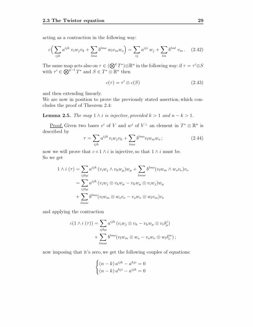
Lemma 2.5. The map 1 ∧ i is injective, provided k > 1 and n− k > 1.
Proof. Given two bases vi of V and wj of V ⊥ an element in T ∗ ⊗ Rn isdescribed by
τ =∑ijh
aijh viwjvh +∑lmo
blmovlwmwo ; (2.44)
now we will prove that c 1 ∧ i is injective, so that 1 ∧ i must be.So we get
1 ∧ i (τ) =∑ijhµ
aijh (viwj ∧ vhwµ)wµ +∑lmoν
blmo(vlwm ∧ wovν)vν
=∑ijhµ
aijh (viwj ⊗ vhwµ − vhwµ ⊗ viwj)wµ
+∑lmoν
blmo(vlwm ⊗ wovν − vowν ⊗ wlvm)vν
and applying the contraction
c(1 ∧ i (τ)) =∑ijhµ
aijh (viwj ⊗ vh − vhwµ ⊗ viδjµ)
+∑lmoν
blmo(vlwm ⊗ wo − vowν ⊗ wlδmν ) ;
now imposing that it’s zero,we get the following couples of equations:(n− k) aijh − ahji = 0
(n− k) ahji − aijh = 0

2.4 Invariant forms on Grassmannians 30
and k blmo − boml = 0
k boml − blmo = 0
which imply(n− k)2 aijh = aijh
andk2 blmo = blmo
which are absurd if k > 1 and n− k > 1.
2.4 Invariant forms on Grassmannians
Cohomology of a compact symmetric space M can be computed using in-variant forms: in fact it can be shown in the same way as for compact Liegroups that
H∗(M) ∼= H∗I (M) , (2.45)
in other words the complex of invariant forms gives rise to a cohomology ringH∗
I (M) which is isomorphic to the DeRham one.Moreover:
Proposition 2.6. For a symmetric space M we have
H∗(M) ∼= (∧
m) θ=0 . (2.46)
Proof.Thanks to the relation
[m , m] ⊂ h (2.47)
the differential d applied to invariant forms is identically zero; then
HkI (M) ∼= (
k∧h⊥) θ=0 ; (2.48)
the result follows from equation (2.45).
Example 2.1. We can calculate directly the cohomology of some low-di-mensional symmetric space using equation (2.48): for example G3(R
6) hasthe isotropy representation isomorphic to Σ2
+ ⊗ Σ2−, where Σ2
± are the spinrepresentations of the factors SU(2)± in SO(4) ∼= SU(2)+SU(2)−; then if2t, 0,−2t and 2s, 0,−2s are the weights of the corresponding sl(2,C) repre-sentations, combining them and then grouping the weight spaces properly, we

2.4 Invariant forms on Grassmannians 31
can decompose the complexified exterior algebra at a point in irreduciblesummands in the following way (thanks to the metric we forget about dis-tinguishing between tangent and cotangent space):
2∧Σ2
+ ⊗ Σ2− ∼= Σ4
+ ⊗ Σ2− + Σ2
+ ⊗ Σ4− + Σ2
+ + Σ2− ; (2.49)
3∧Σ2
+ ⊗ Σ2− ∼= Σ6
+ + Σ6− + Σ4
+ ⊗ Σ4− + Σ4
+ ⊗ Σ2−+ (2.50)
Σ2+ ⊗ Σ4
− + Σ2+ ⊗ Σ2
− + Σ2+ + Σ2
− ; (2.51)4∧
Σ2+ ⊗ Σ2
− ∼= Σ6+ ⊗ Σ2
− + Σ2+ ⊗ Σ6
− + Σ4+ ⊗ Σ4
− + Σ4+ ⊗ Σ2
−+ (2.52)
Σ2+ ⊗ Σ4
− + Σ4+ + Σ4
− + 2 Σ2+ ⊗ Σ2
− + C . (2.53)
In conclusion we have b1 = b2 = b3 = b6 = b7 = b8 = 0 and b0 = b4 = b5 =b9 = 1. With a bit more of work we can obtain an explicit expression for theinvariant 4-form Φ that generates H4(G3(R
6)); in fact consider two bases ofthe Σ2
± given by Y+, H+, X+ and Y−, H−, X− satisfying
[Y±, H±] = 2Y± , [Y±, X±] = −H± , [H±, X±] = 2X± ; (2.54)
then we introduce the following notation:
α1 := X+ ⊗X− , α2 := X+ ⊗H− , α3 := X+ ⊗ Y− etc., (2.55)
which are a basis for TxG3(R6)⊗C; then restricting the representation to the
Cartan subalgebra inside sl(2,C)+ × sl(2,C)− we have the following corre-spondence of weights:
α1 α2 α3
α4 α5 α6
α7 α8 α9
−→2t+ 2s 2t 2t− 2s
2s 0 −2s
−2t+ 2s −2t −2t− 2s
;
∧4 Σ2+ ⊗Σ2
− is 126-dimensional, nevertheless the invariant form must be con-tained in the 10-dimensional subspace of weight 0, so we restrict our attentionto this last one; a basis is given by
β1 := α1289 , β2 := α2378 , β3 := α1469 , β4 := α3647 , β5 := α2846 , (2.56)
β6 := α1937 , β7 := α1568 , β8 := α3548 , β9 := α7526 , β10 := α9524 ; (2.57)
so the invariant form is a linear combination
Ω =
10∑i=1
aiβi . (2.58)

2.4 Invariant forms on Grassmannians 32
To obtain the coefficients we impose the condition adY Φ = 0, which impliesthe following set of equations:⎧⎪⎪⎨⎪⎪⎩
−2a1 + a6 = 0 , −2a2 + a6 = 0 , a3 − 2a5 + 2a10 = 0,
a3 − 2a7 = 0 , a4 + 2a9 = 0 , a4 − 2a8 + 2a5 = 0,
a5 + a9 + a7 = 0 , a8 + a10 = 0
with solutions
a1 = a2 = a6/2 , a3 = a4 = −2a10 , a5 = 0 ,
a7 = a8 = −a10 , a9 = a10 .
Imposing the additional condition adY ′Φ = 0 we have the following system:⎧⎪⎪⎨⎪⎪⎩a1 − 2a5 − 2a10 = 0 , a1 + 2a7 = 0 , a2 + 2a8 = 0,
a2 + 2a5 − 2a9 = 0 , 2a3 + a6 = 0 , −2a4 − a6 = 0,
a5 − a7 + a8 = 0 , a9 − a10 = 0
and the intersection of the solutions gives, imposing a1 = 1,
a1 = 1, a2 = 1, a3 = −1, a4 = −1, a5 = 0, a6 = 2, (2.59)
a7 = 1/2, a8 = −1/2, a9 = 1/2, a10 = 1/2 . (2.60)
We want now to go back to the real exterior algebra, so we introduce thereal structures of Σ2
±: the real subrepresentations preserved by the real com-pact groups SU(2)± have as orthonormal bases e1, e2, e3 and f1, f2, f3satisfying
[e1 , ej ] =√
2ek [f1 , fj ] =√
2fk (2.61)
for ijk consequent indices (modulo 3); the relations with the bases in thecomplexified representations are expressed by:
X =1√2(e1 − ıe2) , Y = − 1√
2(e1 + ıe2) , H = −ı
√2e3 , (2.62)
and analogous equations for X ′, H ′, Y ′; definig a basis of the real tangentspace as
w1 := e1 ⊗ f1 , w2 := e1 ⊗ f2 , w3 := e1 ⊗ f3 etc., (2.63)
and substituting in the expression (2.58) using relations (2.62), we obtain, upto a constant, the form
Ω =w3652 − w3614 − w5478 + w1278 + w5214 (2.64)
+ w1937 + w5968 + w2938 + w4967 . (2.65)

2.4 Invariant forms on Grassmannians 33
In this way we can in theory always obtain the Poincare polynomial andan explicit expression for the corresponding invariant forms of any compactsymmetric space, but of course calculations become more messy as dimen-sion increases. Nevertheless in the case of Grassmannians of 3-planes inRn, which are our main object of interest, some more considerations can leadto determine invariant 4-forms in a more straightforward way: in fact thecomplexified isotropy representation in that case is
Σ2 ⊗W = (R3 ⊗ Rn−3) ⊗ C (2.66)
with Σ2 and W = Cn−3 the standard representations of SO(3) and SO(n−3); then
2∧(Σ2 ⊗W ) ⊃ ( 2∧
Σ2)⊗ S2W ⊃ Σ2 ⊗ 〈k〉 ∼= Σ2 , (2.67)
where k denotes the invariant symmetric tensor corresponding to the Killingform; therefore we have
4∧(Σ2 ⊗W ) ⊃ Σ0 (2.68)
spanned by
Ω =3∑
i=1
ωi ∧ ωi , (2.69)
where the ωi are a basis for(∧2 Σ2
) ⊗ S2W ; we will call this form the Na-gatomo 4-form ([64]). Thus in this type of Grassmannians we always havean invariant 4 form, and hence b4 ≥ 1 (see [32] and the observation below).We can describe the Nagatomo 4-form of G3(R
n) for any n in the followingway:we fix an ON basis e1, e2, e3 of R3 = [Σ2] as before, and an ON basisf1, · · · fk of Rk, with k = n − 3; therefore the tangent space TxG3(R
k) isgenerated by
w1 = e1 ⊗ f1, · · · , w3k = e3 ⊗ fk ; (2.70)
from now on we will adopt the convention of separating indices by a comma,to avoid confusion due to double digits indices. In these terms we have:
Proposition 2.7. Let w1, · · · , w3k the ON basis of the isotropy representa-tion of G3(R
n) given in (2.70); then the Nagatomo 4-form Ω in terms of thisbasis is
Ω =2∑
l=0
k+lk∑i=1+lk
k+lk∑j=i+1
wi, i+k, j, j+k (2.71)
where indices are cyclic modulo 3k.
2.4 Invariant forms on Grassmannians 34
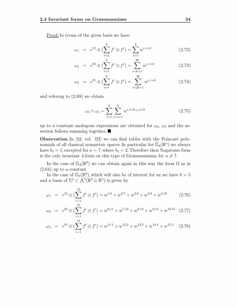
Proof. In terms of the given basis we have
ω1 = e12 ⊗ (
k∑i=1
f i ⊗ f i) =
k∑i=1
wi, i+k (2.72)
ω2 = e23 ⊗ (
k∑i=1
f i ⊗ f i) =
2k∑i=k+1
wi, i+k (2.73)
ω3 = e31 ⊗ (
k∑i=1
f i ⊗ f i) =
3k∑i=2k+1
wi, i+k (2.74)
and referrng to (2.69) we obtain
ω1 ∧ ω1 =k∑
i=1
k∑j=i+1
wi, i+k, j, j+k (2.75)
up to a constant; analogous expressions are obtained for ω2, ω3 and the as-sertion follows summing together.Observation. In [32, vol. III] we can find tables with the Poincare poly-nomials of all classical symmetric spaces. In particular for G3(R
n) we alwayshave b4 = 1, excepted for n = 7,where b4 = 2.Therefore then Nagatomo formis the only invariant 4-form on this type of Grassmannians, for n = 7.
In the case of G3(R6) we can obtain again in this way the form Ω as in
(2.64), up to a constant.In the case of G3(R
8), which will also be of interest for us, we have k = 5and a basis of Σ2 ⊂ ∧2(R3 ⊗ R5) is given by
ω1 = e12 ⊗ (
15∑i=1
f i ⊗ f i) = w1,6 + w2,7 + w3,8 + w4,9 + w5,10 (2.76)
ω2 = e23 ⊗ (
15∑i=1
f i ⊗ f i) = w6,11 + w7,12 + w8,13 + w9,14 + w10,15 (2.77)
ω3 = e31 ⊗ (15∑i=1
f i ⊗ f i) = w11,1 + w12,2 + w13,3 + w14,4 + w15,5 (2.78)

2.4 Invariant forms on Grassmannians 35
In this case the invariant 4-form Ω is given by
Ω =
3∑i=1
ωi ∧ ωi = w1,6,2,7 + w1,6,3,8 + w1,6,4,9 + w1,6,5,10 + w2,7,3,8 (2.79)
+ w2,7,4,9 + w2,7,5,10 + w3,8,4,9 + w3,8,5,10 + w4,9,5,10
+ w6,11,7,12 + w6,11,8,13 + w6,11,9,14 + w6,11,10,15 + w7,12,8,13
+ w7,12,9,14 + w7,12,10,15 + w8,13,9,14 + w8,13,10,15 + w9,14,10,15
+ w11,1,12,2 + w11,1,13,3 + w11,1,14,4 + w11,1,15,5 + w12,2,13,3
+ w12,2,14,4 + w12,2,15,5 + w13,3,14,4 + w13,3,15,5 + w14,4,15,5 .
Chapter 3
Functionals on G3(g)
In this Chapter we consider Grassmannians of 3-planes of a compact Lie alge-bra g: the richness of these latter objects allows to introduce more structurewhich would not be possible with a simple vector space Rn; in particular thestandard 3-form f induces a well-known Morse-Bott function on G3(g), whosegradient flow identifies submanifolds which carry a Quaternionic-Kahler struc-ture, even if this aspect will not be considered until Chapter 5. We shalldefine here a new functional g which will have significance regarding thequaternionic structure.We compare the Hessians of f and g at the criticalpoints for f , finding explicit expressions for the eigenvalues of Hess g. Anearly question that presented itself was whether the critical points of g co-incide with those of f : a negative answer is provided Section 3.4, presentingexplicit examples, and more systematically in Section 3.5.
3.1 The functional f
Consider the Grassmannian of oriented three-planes of a compact semisimpleLie algebra
G3(g)
equipped with the Riemannian metric coming from the Ad-invariant innerproduct on the Lie algebra 〈 , 〉 (minus the Killing form); from now on wewill write G3(g) instead of G3(g) to simplify the notation, or simply G3. Theclosed 3-form
ρ( 〈 , 〉 ) = 〈 [x, y] , z 〉, (3.1)
obtained from the metric through the Cartan map induces a function f onthe Grassmannian (see 1.98): in fact if v1, v2, v3 is an orthonormal basis of

3.1 The functional f 37
the 3-plane V with respect to the inner product then we put
f(V ) := 〈[v1 , v2] , v3〉 (3.2)
which is well defined: in fact the space V is isomorphic to [Σ2] as an SO(3)representation, so that
∧3 V ∼= ∧3[Σ2] ∼= [Σ0], and any element (proportionalto the volume form) is SO(3) invariant.
Let us calculate the gradient vector field obtained as the dual of df viathe metric: we define
w1 = [v2 , v3]⊥ (3.3)
w2 = [v3 , v1]⊥ (3.4)
w3 = [v1 , v2]⊥ (3.5)
so that
[v1, v2] = 〈 [v1, v2] , v3 〉 + w3 (3.6)
[v2, v3] = 〈 [v2, v3] , v1 〉 + w1 (3.7)
[v3, v1] = 〈 [v3, v1] , v2 〉 + w2 (3.8)
Observation. Recall that invariance of 〈 , 〉 implies
〈 [a, b] , c 〉 = 〈 a, [b , c] 〉 . (3.9)
An explicit expression for df is so obtained in the following lemma:
Lemma 3.1. We have
(grad f)V =
3∑i=1
vi ⊗ wi . (3.10)
Proof. Let us consider a curve V (t) ⊂ G3(g) such that V (0) = V definedby
(v1 + tp1, v2 + tp2, v3 + tp3)
where pi ∈ V ⊥ then we have
f(V (t)) = 〈 [v1 + tp1, v2 + tp2] , v3 + tp3 〉 = (3.11)
= f(V ) + t(〈 [p1, v2] , v3] 〉 + 〈 [v1, p2] , v3] 〉+ (3.12)
+ 〈 [v1, v2] , p3] 〉) +O(t2) (3.13)
and so, using 3.9
d
dtf(V (t))|t=0 =
3∑i=0
〈wi, pi 〉 (3.14)
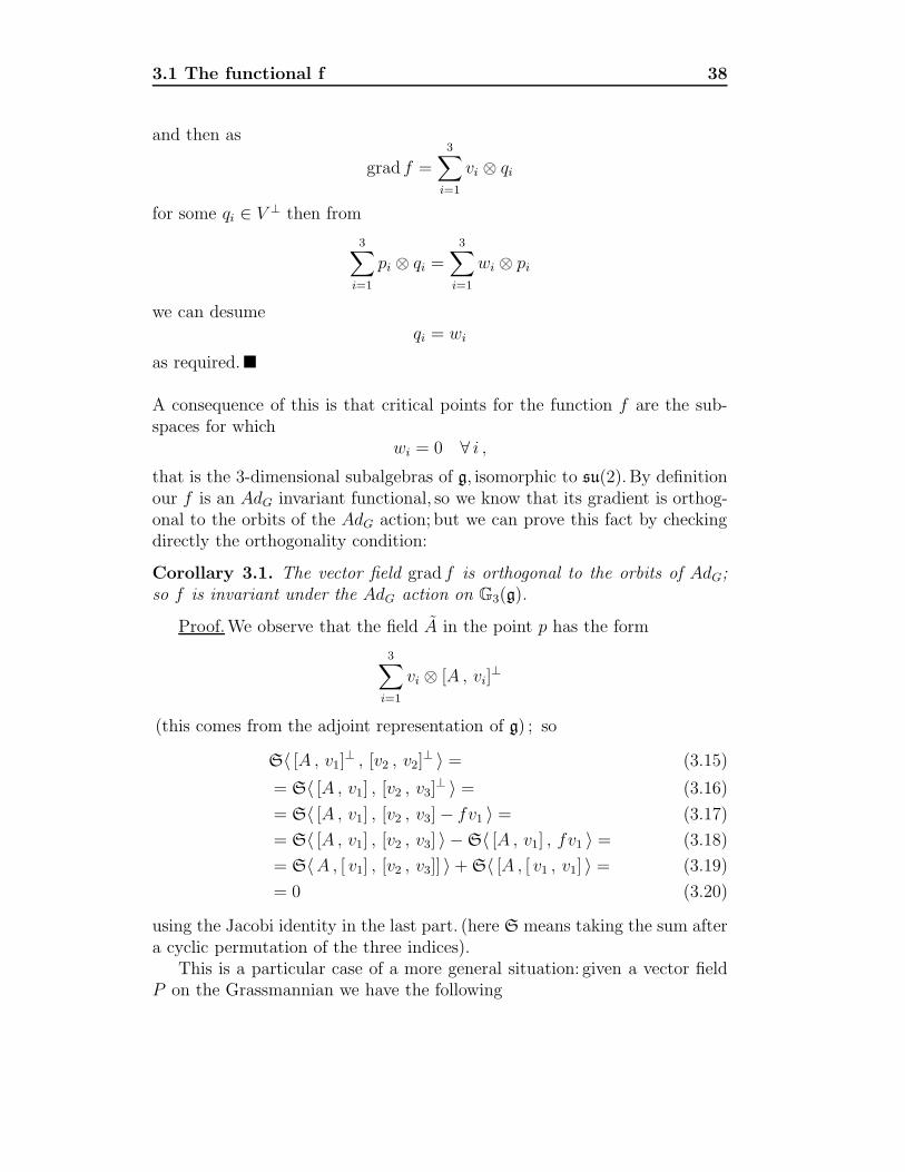
3.1 The functional f 38
and then as
grad f =
3∑i=1
vi ⊗ qi
for some qi ∈ V ⊥ then from
3∑i=1
pi ⊗ qi =3∑
i=1
wi ⊗ pi
we can desumeqi = wi
as required.
A consequence of this is that critical points for the function f are the sub-spaces for which
wi = 0 ∀ i ,that is the 3-dimensional subalgebras of g, isomorphic to su(2). By definitionour f is an AdG invariant functional, so we know that its gradient is orthog-onal to the orbits of the AdG action; but we can prove this fact by checkingdirectly the orthogonality condition:
Corollary 3.1. The vector field grad f is orthogonal to the orbits of AdG;so f is invariant under the AdG action on G3(g).
Proof.We observe that the field A in the point p has the form
3∑i=1
vi ⊗ [A , vi]⊥
(this comes from the adjoint representation of g) ; so
S〈 [A , v1]⊥ , [v2 , v2]
⊥ 〉 = (3.15)
= S〈 [A , v1] , [v2 , v3]⊥ 〉 = (3.16)
= S〈 [A , v1] , [v2 , v3] − fv1 〉 = (3.17)
= S〈 [A , v1] , [v2 , v3] 〉 − S〈 [A , v1] , fv1 〉 = (3.18)
= S〈A , [ v1] , [v2 , v3]] 〉 + S〈 [A , [ v1 , v1] 〉 = (3.19)
= 0 (3.20)
using the Jacobi identity in the last part. (here S means taking the sum aftera cyclic permutation of the three indices).
This is a particular case of a more general situation: given a vector fieldP on the Grassmannian we have the following

3.1 The functional f 39
Definition 3.1. We define the projection map
γ : TpG3 → g (3.21)
acting as
γ(P ) :=3∑
i=1
[vi , pi] (3.22)
where the pi are the orthogonal components of the vector field at p.
The map γ(P ) can be interpreted as a projection on the orbit through apoint p, in fact we have the following
Lemma 3.2. Let A ∈ g; let us consider the vector field A associated to the1-parameter group of diffeomorphisms of G3 generated by exp tA through theadjoint action on g; then a vector field P on G3 is orthogonal to the orbit atthe point p if and only if γ(P ) = 0.
Proof.The condition of orthogonality of P is expressed by
0 = 〈 A , P 〉 =
3∑i=1
〈 [A , vi]⊥ , Pi 〉 = (3.23)
=3∑
i=1
〈 [A , vi] , Pi 〉 =3∑
i=1
〈A , [ vi , Pi] 〉 = (3.24)
= 〈A , γ(P ) 〉 . (3.25)
Maximal critical submanifolds
The AdG orbit of a 3-dimensional subalgebra is a homogeneous submanifoldof the form
M =G
N(su(2)), (3.26)
where N(su(2)) is the normalizer of the subalgebra,i.e. N(su(2)) = g ∈g | [g, h] ∈ su(2) ∀h ∈ su(2) . The critical submanifold obtained choosing thecopy of su(2) ⊂ g corresponding to the maximal root is of particular interestfor us; in fact they are isomorphic to compact Wolf sapces (see [83]), the onlyknown examples of compact Quaternion-Kahler manifolds. They are sym-metric spaces of positive scalar curvature, and we will describe them morein detail in the next chapter.We want however point out here a property ofthis type of subalgebras which characterizes their critical submanifolds as themaxima for the flow of grad f .

3.1 The functional f 40
Observation.The functional f changes sign if we reverse the orientation:therefore every critical manifold C such that f(C) > 0 has a specular copyC ′ for whhich f(C ′) < 0; hence for instance Wolf spaces appear both asabsolute maxima and absolute minima.
The property of being a local maximum for f can be deduced by justlooking at the roots diagram of g; to do this, let us recall some facts fromthe classical theory of roots: a Lie algebra can be completely reconstructedfrom the data encoded in the corresponding Cartan matrix or, equivalently,in the corresponding Dynkin diagram; these two entities describe the anglesbetween a couple of simple roots (those such that are a basis of the algebraand respect to which every other root can be expressed as a linear combina-tion with integer coefficients of the same sign). These angles are expressedby coefficients (called Cartan numbers)
nβα := 〈β , α〉 = 2〈β , α〉〈α , α〉
for two roots α and β, with ‖β‖ ≥ ‖α‖; these coefficients moreover allow toreconstruct the α string through β, i.e. the coefficients p, q for which
β − p α, · · · , β + q α
with nβα = p − q is still a root; in Table 3.1 are expressed all the possiblevalues of 〈α , β〉 for any couple of roots, obtained from the relation
nβα = 2 cos θ‖β‖‖α‖ =⇒ nαβnβα = 4 cos2 θ . (3.27)
We have the following proposition, a version of Theorem 4.2 in [83] adap-ted to our needs:
Proposition 3.3. Let su(2) ⊂ g be a 3-dimensional subalgebra correspondingto a root, then the decompositions in su(2) modules of g under the restrictionof the adjoint representation has the form
g ∼= su(2) + h[Σ0] + k[Σ1] , (3.28)
with h, k ∈ N if and only if the root is the maximal one.
Proof. Let β be the maximal root and let α = β be any posotive root; thenα + β is not a root, instead α − β could be a root; finally α − 2β cant’t bea root, otherwise 2β − α = β + (β − α) > β would be a root, which is

3.1 The functional f 41
〈α , β〉 〈β , α〉 θ ‖β‖2/‖α‖2
0 0 π/2 ?
1 1 π/3 1
−1 −1 2π/3 1
1 2 π/4 2
−1 −2 3π/4 2
1 3 π/6 3
−1 −3 5π/6 3
Table 3.1: A list of all the possible values of 〈α , β〉 and the correspondingangles θ.
impossible. So the Cartan integer nαβ can be 0 or 1, or in other words theβ string through α consists of α or α, α − β; now if we choose a vectorX in the negative root space V−β, its adjoint action adX applied to elementsY ∈ Vα kills them after 1 or 2 applications, depending if nα,β is 0 or 1; thisimplies that the nilpotent part of gC is completely decomposed in summandsof type Σ0 or Σ1; regarding the Cartan subalgebra h, it can be decomposedas
h = Hβ ⊕H⊥β , (3.29)
where H⊥β consists of trivial su(2) representations, so again of type Σ0. Vice
versa, let β be a root satisfying (3.28), supposing it is not maximal; we canorder the roots so that β belongs to the closure of the positive Weyl cham-ber, so that 〈α, β〉 ≥ 0 for all α > 0. Then exists a root α > 0 such thatα + β is still a root; now, if 〈α, β〉 = 0 then the β string through α containsat least two elements, if 〈α, β〉 > 0 at least 3; in both cases α belogs to asummand of type Σk with k > 1.Observation. i)This fact, together with the expression for the Hessian of fgiven later (see (3.69)) shows that the Wolf spaces appear as local maxima(minima) for f ;ii) another consequence of roots theory is that in the decomposition of g givenby a copy of su(2) associated to a root, we can obtain summands Σk with kat most 3, because the lenght of any string of roots is at most 4 (see(3.27)).
Actually more can be deduced using the classification of subalgebras dueto Dynkin ([26]): in fact the functional f can be related to the index of a

3.1 The functional f 42
representation p : su(2) → g: this is defined as the number n satisfiyng
〈p(u), p(v)〉g = n〈u, v〉su(2) (3.30)
for u, v ∈ su(2), where 〈·, ·〉(·) denotes the Killing form of the two algebras
normalized in such a way that the highest root has lenght√
2; therefore theindex is the homotethy factor of the representation p with respect to thesemetrics. The relation with f is expressed in the following lemma:
Lemma 3.4. Let su(2) ⊂ g be a subalgebra of index n; then
n =2
f 2(V )(3.31)
with V = su(2).
Proof.Consider an orthonormal basis e1, e2, e3 of su(2) satisfying
[e1, e2] =√
2e3 ; (3.32)
the f is calculated using a basis which is orthonormal with respect to 〈·, ·〉g,so consider the g-normalized basis
ei =ei
‖ei‖g
=ei√n
; (3.33)
then
f(su(2)) = 〈[ p(e1), p(e2)], p(e3)〉g =
√2
n√n〈p(e3), p(e3)〉g (3.34)
=√
2n
n√n〈e3, e3〉su(2) =
√2√n, (3.35)
hence the conclusion.Dynkin showed that the index n is a natural number: a consequence is that
a list of the possible values of f in correspondece of the critical submanifoldsis given by:
±√
2, ±1, ±√
2√3, ± 1√
2, ....etc. (3.36)
Dynkin also showed the following theorem:
Theorem 3.5. Let g a subalgebra of g of index 1; then the maximal root andits root vectors coincide with the maximal root and root vectors of g.
A consequence is the following:
Corollary 3.2. The functional f attains its absolute maximum (minimum,changing orientation) on the Wolf spaces.

3.2 The functional g 43
3.2 The functional g
We define now another functional on the grassmannian which will be usefulin the sequel. We define it as
g(V ) =∑i<j
‖[vi , vj ]‖2 , (3.37)
and observe that it can be written as
g(V ) = 3 f 2 + ‖grad f‖2 . (3.38)
We can describe the field grad g and then use the previous results to showthat it is orthogonal to the AdG orbits; before this we record
Definition 3.2. Let V be a k-dimenional linear subspace of a Lie algebra g
with an ON basis v1, · · · vk; the generalized Casimir operator is a map
C : V g (3.39)
defined as
C(v) =k∑
i=1
(advi)2(v) . (3.40)
This concept generalizes that of the Casimir operatr, which is defined as
C(v) =
k∑i=1
(ρvi)2(v) . (3.41)
where ρ : V → g′ is a representation of a Lie algebra V = g′ in g, andnot a simple vector space.This operator is related to the laplace-Beltramioperator; for an application in a representation-theorethic context see [27].
Going back to g, we have
Proposition 3.6. The gradient of g is
grad g = −23∑
i=1
vi ⊗ C(vi)⊥ , (3.42)
where C is the generalized Casimir operator associated to V .

3.2 The functional g 44
Proof.We have
g(V (t)) =3∑
i<j
‖[vi + tPi , vj + tPj]‖2 = (3.43)
= g(V0) + t(2[v1 , P2] , [v1 , v2] + [P1 , v2] , [v1 , v2]+ (3.44)
+ 2[v2 , P3] , [v2 , v3] + [P2 , v3] , [v2 , v3]+ (3.45)
+ 2[v3 , P1] , [v3 , v1] + [P3 , v1] , [v3 , v1])+ (3.46)
+O(t2) (3.47)
and so
d
dtg(V (t))|t=0 = − 2〈P1 , [v2 , [v2 , v1]] 〉 − 2〈P2 , [v1 , [v1 , v2]] 〉+ (3.48)
− 2〈P3 , [v2 , [v2 , v3]] 〉 − 2〈P2 , [v3 , [v3 , v2]] 〉+ (3.49)
− 2〈P1 , [v3 , [v3 , v1]] 〉 − 2〈P3 , [v1 , [v1 , v3]] 〉 (3.50)
= −2
3∑i=1
〈Pi , C(vi) 〉 , (3.51)
by definition of the Casimir operator; the conclusion follows as for grad f .Observation.A consequence is that the three dimensional subalgebras of g
are critical points for g, as well as for f , but not necessarily all of them.
The next step is proving that g is AdG invariant; this actually followsdirectly from the invariance of 〈, 〉 and of [, ], but but we prove it here tobetter exemplifying the use of the operator γ.
We need the following lemma:
Lemma 3.7. The following identity holds:
3∑i,j=1
[vi , [vj , [vj , vi]]] = 0 .
Proof.We apply the Jacobi Identity to one of the terms of the sum (afternoting that for i = j the term is 0):
0 = [vi , [vj , [vj , vi]]] + [[vj , vi] , [vi , vj]] + [vj , [[vj , vi] , vi]] = (3.52)
= [vi , [vj , [vj , vi]]] + [vj , [vi , [vi , vj]]] ; (3.53)
the conclusion follows immediately.
We are now able to prove the following fact, previously stated.

3.2 The functional g 45
Theorem 3.8. We haveγ(grad g) = 0 , (3.54)
so grad g is orthogonal to the AdG orbits and g is AdG invariant.
Proof.We have
γ(grad g) =3∑
i,j=1
[vi , C(vi)] =3∑
i,j=1
[vi , [vj , [vj , vi]]⊥] ; (3.55)
but by definition
[vj , [vj , vi]]⊥ = [vj , [vj , vi]] −
3∑k=1
〈 [vj , [vj , vi]], vk 〉vk , (3.56)
and then
γ(grad g) =3∑
i,j=1
[vi , [vj , [vj , vi]]]−3∑
i,j,k=1
[vi , 〈 [vj , [vj , vi]], vk 〉vk] ; (3.57)
but the first summand is zero by the previous lemma; so we have to checkthe second summand:more explicitly
3∑i,j,k=1
[vi , 〈 [vj , [vj , vi]], vk 〉vk] = [v1 , 〈 [v2 , [v2 , v1]], v1 〉v1]+
+[v1 , 〈 [v2 , [v2 , v1]], v2 〉v2] + [v1 , 〈 [v2 , [v2 , v1]], v3 〉v3]+
+[v2 , 〈 [v1 , [v1 , v2]], v1 〉v1] + [v1 , 〈 [v1 , [v1 , v2]], v2 〉v2]+
+[v1 , 〈 [v1 , [v1 , v2]], v3 〉v3] + [v1 , 〈 [v3 , [v3 , v1]], v1 〉v1]+
+[v1 , 〈 [v3 , [v3 , v1]], v2 〉v2] + [v1 , 〈 [v3 , [v3 , v1]], v3 〉v3]+
+[v3 , 〈 [v1 , [v1 , v3]], v1 〉v1] + [v3 , 〈 [v1 , [v1 , v3]], v2 〉v2]+
+[v3 , 〈 [v1 , [v1 , v3]], v3 〉v3] + [v3 , 〈 [v2 , [v2 , v3]], v1 〉v1]+
+[v3 , 〈 [v2 , [v2 , v3]], v2 〉v2] + [v3 , 〈 [v2 , [v2 , v3]], v3 〉v3]+
+[v2 , 〈 [v3 , [v3 , v2]], v1 〉v1] + [v2 , 〈 [v3 , [v3 , v2]], v2 〉v2]+
+[v2 , 〈 [v3 , [v3 , v2]], v3 〉v3] =
=〈 [v1 , v2] , [v2 , v3] 〉[v3 , v1] + 〈 [v2 , v1] , [v1 , v3] 〉[v3 , v2]+
+〈 [v1 , v3] , [v3 , v2] 〉[v2 , v1] + 〈 [v3 , v1] , [v1 , v2] 〉[v2 , v3]+
+〈 [v3 , v2] , [v2 , v1] 〉[v1 , v3] + 〈 [v2 , v3] , [v3 , v1] 〉[v1 , v2] =
= 0 .

3.3 Hessians 46
3.3 Hessians
We introduce next some basic language from Morse-Bott theory,which will beuseful in the sequel; then we will study the critical manifolds for the functionalg, in comparison with those of f .
Morse-Bott theory
Morse-Bott theory is a generalization of Morse theory: allowing only the exis-tence of isolated critical points is somewhat restrictive, as for example costantfunctions are not of Morse type; nor it is the height function of a 2-torus lyinghorizontally (the critical manifolds are two circles).Morse-Bott theory fur-nishes a decomposition of the given manifold in terms of cell bundles, relatingits topology to that of critical submanifolds.
A critical submanifold X ⊂ M for a differentiable function f : M −→ R
is said nondegenerate if the 0-eigenspace for the Hessian of f at any point xof X coincides with TxX. The index of a critical manifold X is the dimensionof the negative eigenspace of the Hessian of f at x ∈ X.
Definition 3.3. Let f be a smooth real valued function on a differentiablemanifold M ; if all its critical manifolds are nondegenerate, then we call it aMorse-Bott function.
The Morse-Bott inequalities allow us to estimate the Betti numbers ofthe manifold M with the number of critical manifolds of a fixed index:
Theorem 3.9. The following equality holds:
MB(t) − P (t) = (1 + t)Q(t) , (3.58)
where Q(t) is a polynomial with nonnegative coefficients.
Definition 3.4. A Morse-Bott function is called perfect if
P (t) = MB(t). (3.59)
Theorem 3.9 implies that if MB(t) contains no odd powers, then theMorse-Bott function is authomatically perfect.
The Hessian of g
The functional f is known to be a Morse-Bott function (see (3.69)); insteadnot much is known about the critical manifolds of the functional g; first of allwe determine an expression for the Hessian of g at the critical submanifolds

3.3 Hessians 47
corresponding to subalgebras; in the later sections we will try to find newcritical manifolds for g.
Let us calculate the Hessian of g at a critical point for f , in the samespirit of Proposition 2.2 in [50]:
Proposition 3.10. The eigenvalues of the Hessian of the function g at acritical point for the flow of grad f are decribed by the second degree polyno-mial:
Hg|Σk
= 2f 2(l2 − l − 2) . (3.60)
where l is an integer depending on the degree of the su(2) representation inV ⊥ and V ⊗ V ⊥.
Proof.We have
Hg (X, Y ) =2S (〈 [XY v1 , v2] , [v1 , v2] 〉 + 〈 [Xv1 , Y v2] , [v1 , v2] 〉+ 〈 [v1 , XY v2] , [v1 , v2] 〉 + 〈 [Xv1 , v2] , [Y v1 , v2] 〉+ 〈 [v1 , Xv2] , [v1 , Y v2] 〉 + 〈 [Y v1 , Xv2] , [v1 , v2] 〉+ 〈 [Xv1 , v2] , [v1 , Y v2] 〉 + 〈 [Y v1 , v2] , [v1 , Xv2] 〉) ,
for 24 terms in total.Defining the operator
AX = −1
f
∑j
ad vj X ad vj (3.61)
and grouping the terms in a suitable way we obtain:
2S (〈 [XY v1 , v2] , [v1 , v2] 〉 + 〈 [v1 , XY v2] , [v1 , v2] 〉) =
2S f(〈 [XY v1 , v2] , v3 〉 + 〈 [v1 , XY v2] , v3 〉) =
−2S f(〈 Y v1 , X[v2 , v3] 〉 + 〈 Y v2 , X[v3 , v1] 〉) =
− 4f 2∑
i
〈Y vi , Xvi〉
using 6 terms; then
2S (〈 [Xv1 , Y v2] , [v1 , v2] 〉 + 〈 [Y v1 , Xv2] , [v1 , v2] 〉) =
2S f(〈 [Xv1 , Y v2] , v3 〉 + 〈 [Y v1 , Xv2] , v3 〉) =
2S f(〈Xv1 , [Y v2 , v3] 〉 + 〈 Y v1 , [Xv2 , v3] 〉) =
2S f(〈Xv3 , [Y v1 , v2] 〉 + 〈 Y v1 , [Xv2 , v3] 〉) =
2S f(〈 Y v1 , [v2 , Xv3] − [v3 , Xv2] 〉 =
= − 2f∑
i
〈Y vi , AXvi〉 ,

3.3 Hessians 48
using other 6 terms; finally
2S (〈 [Xv1 , v2] , [Y v1 , v2] 〉 + 〈 [v1 , Xv2] , [Y v1 , v2] 〉)+〈 [Xv1 , v2] , [v1 , Y v2] 〉 + 〈 [v1 , Xv2] , [v1 , Y v2] 〉) =
2S (〈 Y v1 , [v2 , AXv3] 〉 − 〈 Y v2 , [v1 , AXv3] 〉) =
2S f(〈AXv3 , [v2 , Xv1] − [v1 , Xv2] 〉 =
=2∑
i
〈AY vi , AXvi〉 ,
using the last 12 terms; so in conclusion we can write
Hg (X, Y ) =∑
i
−4f 2〈Y vi , Xvi〉 − 2f〈Y vi , AXvi〉 + 〈AY vi , AXvi〉 ;
(3.62)moreover recall that if v1, v2, v3 is an orthonormal basis for te subalgebraisomorphic to su(2) the representation p is not an isometry with respect tothe standard Killing forms, in fact
Bg(p∗vi , p
∗vj) = −2 δij f(V )2 ;
so the Casimir operator Cρ associated to the su(2) representation ρ obtainedfrom the adjoint action of V inside g can be expressed as
Cρ = − 1
2f(V )2
3∑i=1
ρ(vi)ρ(vi) ; (3.63)
this operator acts on the irreducible su(2) representation Σk by multiplicationfor the constant
C(k) =(k + 1)2 − 1
8. (3.64)
The definition of Cp implies the equality
CV ∗⊗V ⊥X = CV ⊥X +XCV +1
fAX (3.65)
so that we haveAX = f(CV ∗⊗V ⊥ − CV ⊥ − 1)X . (3.66)
Then, if X = Y is an element of an orthonormal basis for TV G3 = V ∗ ⊗ V ⊥
belonging to the subrepresentation Σk, defining a new parameter as
l = CV ∗⊗V ⊥ − CV ⊥ − 1 (3.67)

3.3 Hessians 49
-3 -2 -1 1 2 3 4l
-2
-1
1
2
3
4
5
gl,fl
Figure 3.1: The graphs of the Hessians of f and g in function of the parameterl.
depending on the degree of the Σk summand, hence the conclusion.The polynomial in (3.60) has −1 and 2 as zeroes; we observe that -1 is a rootalso for the corresponding polynomial for f : in fact a similar calculation (see[50]) gives
Hf (X, Y ) = −∑
i
f〈Y vi , Xvi〉 + 〈Y vi , AXvi〉 (3.68)
and consequently
Hf|Σk
= −f(l + 1) . (3.69)
Observation:Equation (3.69) implies that f is a Morse-Bott function, see[50].
The following lemma describes some relations between the Hessians ofthe two functionals:

3.3 Hessians 50
Lemma 3.11. Let V = su(2) ⊂ g be a critical point for f ; then: i)the 0-eigenspace for the Hessian of g contains that of the Hessian of f ; the inclusionis strict if and only if su(2)⊥ ⊃ Σ4;
ii)if the corresponding critical manifold is a local maximum (minimum)for f then it is also a local maximum (minimum) for g .
Proof. i)Equation (3.60) implies that a sufficient condition for the Hessianof g being 0 is that
CV ∗⊗V ⊥ − CV ⊥ = 0 , (3.70)
and this happens exactly in the middle term of the tensor product of su(2)representations that describe the tangent space at V :
Σ2 ⊗ Σk = Σk+2 + Σk + Σk−2 ; (3.71)
this is consistent with the fact that critical manifolds for f are also criticalfor g; but the condition is not necessary, for the presence of the second root2: for example, as we shall see later, in the so(3) critical manifold for su(3)other directions have 0 as eigenvalue for the Hessian of g; in fact CΣ6 is themultiplication for 6, so
CΣ6 − CΣ4 − 1 = 6 − 3 − 1 = 2 . (3.72)
This last condition is satisfied if and only if k = 4: in fact we are asking that
l = CV ∗⊗V ⊥ − CV ⊥ − 1 = 2 (3.73)
which is equivalent to write
l =(k + 2 + 1)2 − 1
8− (k + 1)2 − 1)2
8− 1 = 2 (3.74)
if and only ifk2 + 2k + 8
8− k2 + 2k
8− 1 = 2 (3.75)
if and only ifk = 4 ; (3.76)
so we can have another 0 eigenspace for the Hessian of g if and only if
V ⊥ ⊃ Σ4 . (3.77)
ii)We note first that at a local minimum for f with f < 0 the condition
l + 1 ≥ 0 (3.78)

3.4 Low dimensional examples 51
has to be satisfied, but this means that
CV ∗⊗V ⊥ − CV ⊥ ≥ 0 ; (3.79)
this happens if and only if (see also (3.3))
V ⊥ = aΣ0 + bΣ1 , a, b ∈ N (3.80)
so that in consequence we have
Hg = −4f 2 or Hg = −9
4f 2 , (3.81)
on the normal bundle, so that V is a local maximum for g. On the other handwe can’t have local minima for f when f > 0 because for analogous reasonsthe decompositon of the tangent space should not contain irreducible su(2)modules of dimension grater than the ones in V ⊥, but this is impossible.Wecan obtain all local maxima for f just reversing the orientation of a min-imum, so that for what we have just said they are maxima also for g, theconclusion follows.
3.4 Low dimensional examples
We are going now to study more in detail the Hessians of the two functionalsf, g on the Grassmannians of 3-planes of some low dimensional classical Liealgebras.
The Lie algebra u(2)
We know that critical manifolds for f are also critical for g; it’s quite naturalto ask ourselves if these are all of them; the answer is no. In fact for examplelet us consider the case of u(2): we have the orthogonal decomposition
u(2) = R ⊕ su(2) ,
where the R factor (generated by an element h) kills everything under ad-joint action; the known critical manifolds inside the Grassmannian G3(u(2))(isomorphic to S3) are the ones corresponding to the copy of su(2) with thetwo orientations (with normalizer the whole algebra, so isolated points); theseare the absolute maximum and minimum for f , but only local maxima forg; this consideration implies the existence of other critical points. In fact letus consider the 3 dimensional subspace V generated by h, a1, a2, where the
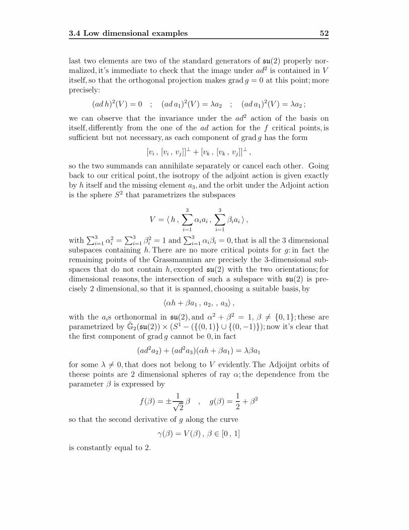
3.4 Low dimensional examples 52
last two elements are two of the standard generators of su(2) properly nor-malized, it’s immediate to check that the image under ad2 is contained in Vitself, so that the orthogonal projection makes grad g = 0 at this point;moreprecisely:
(ad h)2(V ) = 0 ; (ad a1)2(V ) = λa2 ; (ad a1)
2(V ) = λa2 ;
we can observe that the invariance under the ad2 action of the basis onitself, differently from the one of the ad action for the f critical points, issufficient but not necessary, as each component of grad g has the form
[vi , [vi , vj ]]⊥ + [vk , [vk , vj]]
⊥ ,
so the two summands can annihilate separately or cancel each other. Goingback to our critical point, the isotropy of the adjoint action is given exactlyby h itself and the missing element a3, and the orbit under the Adjoint actionis the sphere S2 that parametrizes the subspaces
V = 〈 h ,3∑
i=1
αiai ,
3∑i=1
βiai 〉 ,
with∑3
i=1 α2i =
∑3i=1 β
2i = 1 and
∑3i=1 αiβi = 0, that is all the 3 dimensional
subspaces containing h. There are no more critical points for g: in fact theremaining points of the Grassmannian are precisely the 3-dimensional sub-spaces that do not contain h, excepted su(2) with the two orientations; fordimensional reasons, the intersection of such a subspace with su(2) is pre-cisely 2 dimensional, so that it is spanned, choosing a suitable basis, by
〈αh+ βa1 , a2, , a3〉 ,with the ais orthonormal in su(2), and α2 + β2 = 1, β = 0, 1; these areparametrized by G2(su(2)) × (S1 − ((0, 1) ∪ (0,−1)); now it’s clear thatthe first component of grad g cannot be 0, in fact
(ad2a2) + (ad2a3)(αh+ βa1) = λβa1
for some λ = 0, that does not belong to V evidently. The Adjoijnt orbits oftheese points are 2 dimensional spheres of ray α; the dependence from theparameter β is expressed by
f(β) = ± 1√2β , g(β) =
1
2+ β2
so that the second derivative of g along the curve
γ(β) = V (β) , β ∈ [0 , 1]
is constantly equal to 2.

3.4 Low dimensional examples 53
Σ2 Σ4 Σ6
C 1 3 6
Hf −√2 0 3/
√2
Hg 10 0 0
Table 3.2: The Hessians at so(3) ⊂ su(3)
Σ1 Σ2 Σ3
C 3/8 1 15/8
Hf 0√
2 3/√
2
Hg 0 −8 −9
.
Table 3.3: The Hessians at su(2) ⊂ su(3)
The Lie algebra su(3)
The following tables describe the behaviour of the two Hessians at the criticalpoints for f : at so(3) (with f = − 1√
2and g = 3
2) we have the decomposition
Tso(3)G3 = Σ2 ⊗ Σ4 = Σ2 + Σ4 + Σ6 , (3.82)
and the eigenvalues of the Hessians are reported in Table 3.2; instead atsu(2) ⊂ su(2), with f = −√
2 and g = 6,where the decomposition of thetangent space is given by
Tsu(2)G3 = Σ2 ⊗ (Σ0 + 2Σ1) = Σ2 + 2Σ1 + 2Σ3 (3.83)
we have the Hessians of the two functions taking the values as in Table 3.3.The last 0 in the last row of Table 3.2 could be interpreted as a degeneracy
of the Hessian of g, so that it would not be a Morse-Bott function, or it couldmean that the critical manifold for g strictly contains the one of f . We nowrecall the decomposition of su(3) under the adjoint action restricted to theCartan subalgebra h of the diagonal elements:
su(3) = h ⊕ gα ⊕ gβ ⊕ gα+β , (3.84)
where gα denotes the 2 dimensional real space generated by elements of theform (gα − g−α) and ı(gα + g−α),α being a root; the Adjoint action of themaximal torus corresponding to h is essentially a u(1) action on each of

3.4 Low dimensional examples 54
these summands: in fact the kernel of the corresponding root in h, which isa hyperplane, is tangent in general to a rank(g)− 1 dimensional torus whichis the stabilizer of a point of the maximal torus representation.
It is straightforward to prove that the 3-dimensional torus T3
V = 〈 1√2
⎛⎝ 0 eıs 0−e−ıs 0 0
0 0 0
⎞⎠ ,1√2
⎛⎝0 0 00 0 eıt
0 −e−ıt 0
⎞⎠ ,1√2
⎛⎝ 0 0 eıu
0 0 0−e−ıu 0 0
⎞⎠ 〉
for s, t, u ∈ R identifies 3-dimensional subspaces that are closed under thesquared adjoint action mutually applied between the generators, as usual, sothat grad g = 0 at V ; we observe that these subspaces are not subalgebrasexcepted when the parameters satisfy the condition
s+ t− u = kπ (3.85)
for which we get the intersection of T3 with the orbit of so(3) under theAdjoint action; the restriction of f to this submanifold is expressed by
f(s, t, u) =1√2
cos (s+ t− u) (3.86)
so that the intersection with the fibres is given by the 2 dimensional toris+ t− u = const; instead we have
g =3
2(3.87)
constantly.
Observation.This explains partially the apparent degeneracy of the Hessianof g (here we have one new degeneracy direction,while the 0-eigenspace forHg is S6 which is 7-dimensional as seen in Table 3.2).
The kernel of the adjoint action (that is the “normalizer” of V ) at thepoints of the torus is precisely so(3) for the subalgebras, giving the alreadyknown critical manifold
SSU (3 ) = SU(3)/SO(3) ; (3.88)
instead it is trivial at all other points: in fact the Cartan subalgebra h is neverin the kernel, as it acts as a rotation in the spaces gα; on the other hand thethree generators of V preserve V itself if and only if V is a subalgebra; in theend, the elements orthogonal to these last ones, with corresponding parame-ters
s′ = s + π/2 , t′ = t+ π/2 , u′ = u+ π/2

3.4 Low dimensional examples 55
Σ2
C 1
Hf√
2
Hg −8
Table 3.4: The Hessians at su(2) ⊂ so(4)
satisfy the condition (ad v1(s′))(v1(s)) ∈ h for example, so they don’t preserve
the space too. So, in conclusion, if s+t−u = kπ the Adjoint orbit is the wholeSU(3).
The Lie algebra so(4)
Inside so(4) we can find essentially three copies of su(2) (for a total of 6 con-sidering the orientation): two corresponding to the standard decomposition
so(4) = su(2) ⊕ su(2) (3.89)
so that we get the decomposition
Σ2 ⊗ (Σ0 + Σ0 + Σ0) = Σ2 + Σ2 + Σ2 (3.90)
and the Hessians at theese points (which are the maxima and the minima forf), take the values reported in Table 3.4. The two functions assume valuesf(su(2)) = −√
2 and g(su(2)) = 6.
The other critical point for f is the diagonal subalgebra su(2)∆; the valuesof our functions are respectively f(su(2)∆) = −1 and g(su(2)∆) = 3; thedecomposition of the tangent space is given by:
Σ2 ⊗ Σ2 = Σ4 + Σ2 + Σ0 (3.91)
and the behaviour of the Hessians is described in Table 3.5. This tells usfor example that this cannot be the absolute minimum for g, and suggeststhat we can find other critical manifolds for it. In fact for example it is easyto check that the following subspaces are critical for g; actually this is just aconsequence of the functoriality respect to the immersion of subalgebras, inparticular for the immersion of u(2): if vi denotes an orthonormal basis ofsu(2) the space
V = 〈(v1 , 0) , (v2 , 0) , (0 , v3)〉 (3.92)

3.4 Low dimensional examples 56
Σ0 Σ2 Σ4
C 0 1 3
Hf −1 0 2
Hg 8 0 −4
Table 3.5: The Hessians at su(2)∆ ⊂ so(4)
comes from the immersion
su(2) ⊕ R → su(2) ⊕ su(2) (3.93)
with values f(V ) = 0 and g(V ) = 2;moreover the kernel of the adjoint actionon V is given by the abelian subalgebra
u(1) × u(1) = 〈(v3 , 0) , (0 , v3)〉 (3.94)
so that the Adjoint orbit isSO(4)/T 2 ; (3.95)
on the other hand the diagonal immersion
su(2) ⊕ R∆→ su(2) ⊕ su(2) (3.96)
has associated the space
W = 〈(v1 , v1) , (v2 , v2) , (v3 , −v3)〉with values f(W ) = 0 and g(W ) = 3; in this case the kernel of the adjointaction is
su(2) = 〈(v1 , −v1) , (v2 , −v2) , (v3 , v3)〉 (3.97)
and the Adjoint orbit is then
SO(4)/O(3) = RP3 . (3.98)
The Lie algebra so(5)
The decomposition at the maximal critical manifold, corresponding to thelong root, is given by
so(5) = su(2) + 2Σ1 + 3Σ0 (3.99)

3.5 New critical manifolds for gradg 57
Σ0 Σ2 Σ4 Σ2
C 0 1 3 1
Hf −1 0 2√
2
Hg 8 0 −4 −8
.
Table 3.6: The Hessians at su(2)∆ ⊂ so(5)
and the tangent space is
TC
su(2)∆G3(so(5)) ∼= Σ2 ⊗ (2Σ1 + 3Σ0) = 2(Σ3 + Σ1) + 3Σ2 (3.100)
where 2Σ1 is tangent to HP1, and the remaining summands are the sta-ble part: the Hessians in fact behave in the same way described in Table3.3, because the representations involved are the same (but with differentmultuplicities), see (3.83).
The decomposition associated to the next to minimal critical manifold, orin other words to the copy su(2)∆ corresponding to the short root, is givenby
so(5) = su(2)∆ + Σ0 + 2Σ2 (3.101)
so that
TC
su(2)∆G3(so(5)) ∼= Σ2 ⊗ (Σ0 + 2Σ2) = 2(Σ4 + Σ0) + 3Σ2 (3.102)
and the eigenvalues of the Hessians are described in Table 3.6.
Observation.The Σ2 column comes from the Σ0 summand of the decompo-sition of V ⊥, so that the values of the Hessians are different with respect tothe Σ2 coming from the Σ4 summand even if they are isomorphic represen-tations, exemplifying the dependence of the parameter l from both V ⊗ V ⊥
and V ⊥ (see (3.67)).
3.5 New critical manifolds for gradg
Critical points for g provide some kind of “generalized subalgebras”, in thesense that
grad f = 0 =⇒ grad g = 0 ; (3.103)
we have already shown in the previous sections that the converse is nottrue, analyzing in detail examples of compact Lie algebras.

3.5 New critical manifolds for gradg 58
Another approach for finding g critical points that are not subalgebrasis looking at the root structure, using the same type of arguments used toprove Proposition 3.3.
Let us consider the case that 〈β , α〉 = −2 for two simple roots; thishappens precisely in so(2n + 1), sp(n) and f(4). This means essentially thatα + β and 2α + β are the only roots belonging to the α string throughβ (β − α is never a root if they are both simple).Now we can consider the3 dimensional space V generated by elemnts of norm 1 taken in the spaces(gα−g−α), (gβ−g−β) and (g2α+β−g−(2α+β)); if we perform the double adjointaction of one generator on the other, keeping in mind that
[gα , gβ] ⊂ gα+β (3.104)
we fall in the same subspaces: in fact we have to take in account that thefollowing are not roots:
2(α+ β) , α + 2β , 3α + 2β ,
the last one because every root of level m can be obtained from one oflevel m − 1 by just adding one simple root; but nor 2(α + β) nor 3α + βare roots in our situation. So taking the orthogonal projection as usual thegradient of g annihilates; this is not a subalgebra, as α+ β stands in V ⊥. Inparticular consider sp(2): a subspace of this kind gives origin, as for su(3), toa 3 dimesnional torus described in terms of matrices (not normalized) by⎛⎜⎜⎝
0 0 eıs 00 0 0 0
−e−ıs 0 0 00 0 0 0
⎞⎟⎟⎠ ,
⎛⎜⎜⎝0 0 0 00 0 0 eıt
0 0 0 00 −e−ıt 0 0
⎞⎟⎟⎠ ,
⎛⎜⎜⎝0 eıu 0 0
−e−ıu 0 0 00 0 0 e−ıu
0 0 −eıu 0
⎞⎟⎟⎠corresponding respectively to β, 2α+ β and α. This torus is contained in thefibres f−1(0) and g−1(1), and doesn’t contain any subalgebra.
Lie Triple Systems
Another possible approach for trying to understand g critical manifolds isthrough the so called Lie Triple Systems (from now on LTS), i.e. thosesubspaces V of a Lie Algebra which satisfy the condition
[X , [Y , Z]] ∈ V ∀X, Y, Z ∈ V ; (3.105)
we quote here a result which links LTS to totally geodesic submanifolds of asymmetric space (see [35]):

3.5 New critical manifolds for gradg 59
Proposition 3.12. Let M = G/K be a Riemannian gobally symmetricspace; let n ⊂ m be a LTS; put N = Exp n. Then N has a natural differ-entiable structure in which it is a totally geodesic submanifold of M with nas tangent space. On the other hand if N is a totally geodesic submanifoldof M and n is the tangent space at some point, then it is a LTS.
We remark that N is a globally symmetric space too, of the form G′/K ′,where G′ is a closed subgroup of G and K ′ = K ∩G′.We are now in positionto state the following criterion for identifying critical submanifolds for grad gwhich are not critical for grad f , or in other words which do not correspond tosubalgebras: recall that grad g = 0 is equivalent to the set of three equations
[vi, [vi, vk]]⊥ + [vj, [vj , vk]
⊥ = 0 (3.106)
for i, j, k = 1, 2, 3 modulo ciclyc permutations; then we have:
Proposition 3.13. Let G be a compact Lie group with Lie algebra g andlet M = G/K be a symmetric space; then any 3-dimensional totally geodesicsubmanifold N corresponds to a critical submanifold in G3(g) for grad g whichis not critical for grad f .
Proof.Proposition (3.12) translates the condition of being a totally geo-desic submanifold to the algebraic condition of a LTS; this clearly impliesthat V satisfies equations (3.106) ; moreover a LTS cannot be a subalge-bra, as V ⊂ m implies
[u, v] ∈ h ⊂ V ⊥ (3.107)
for property (1.16) of symmetric spaces; the Adjoint orbit of the LTS doesnot depend on the base point chosen in N .
For a classification of totally geodesic submanifolds of symmetric spacessee [18] and [19].
We go now do describe some examples: we start with the decomposition
so(5) = so(4) ⊕ m (3.108)
which corresponds to the symmetric space
SO(5)/SO(4) = S4 ; (3.109)
the decomposition can be written in terms of the roots structure in the fol-lowing way (as usual we shall denote gα the 2-dimensional subspace generatedby (gα − g−α) and ı(gα + g−α) and with t the Cartan subalgebra):
so(5) = (t + gβ + g2α+β) + (gα + gα+β) (3.110)

3.5 New critical manifolds for gradg 60
where α and β are simple roots labelled consistently with the previous sec-tion; so
Tp S4 = gα + gα+β (3.111)
and every 3 dimensional totally geodesic subanifolds is a maximal S3; butbeing this a rank 1 symmetric space, that means that the isotropy (Adjoint)representation of SO(4) on Tp S
4 is transitive on the unit vectors, and beingall 3 dimensional subspaces of the tangent space identified by the orthogonalunit vector, we can essentially obatin all elements in the same Adjoint orbitin this way.We choose just to fix the ideas the space
V = gα + (gα+β − g−(α+β)) , (3.112)
and one can check directly that it satisfies the required condition.The valuesof our functions are at this point
f(V ) = 0 , g(V ) = 3 . (3.113)
In this way we can give a different interpretation of the critical point foundin the previous section; in fact we can consider the decomposition
sp(2) = (t + gα+β) + (gα + gβ + g2α+β)
= (R ⊕ su(2)) ⊕ 2Σ2
corresponding to the symmetric space
Sp(2)
SU(2)U(1); (3.114)
the 3 dimensional subspace
V = (gα − g−α) + (gβ − g−β) + (g2α+β − g−(2α+β)) (3.115)
satisfies the definition of LTS, so can be thought as the tangent space of atotally geodesic submanifold of this last one.
Now let us go back to su(3): we can decompose it as a symmetric pair as
su(3) = (t ⊕ gα+β) + (gα + gβ)
= (R ⊕ su(2)) ⊕ 2Σ1 (3.116)
and for example if we choose the 3 dimensional subspace in 2Σ1
V = gα + (gβ − g−β) (3.117)
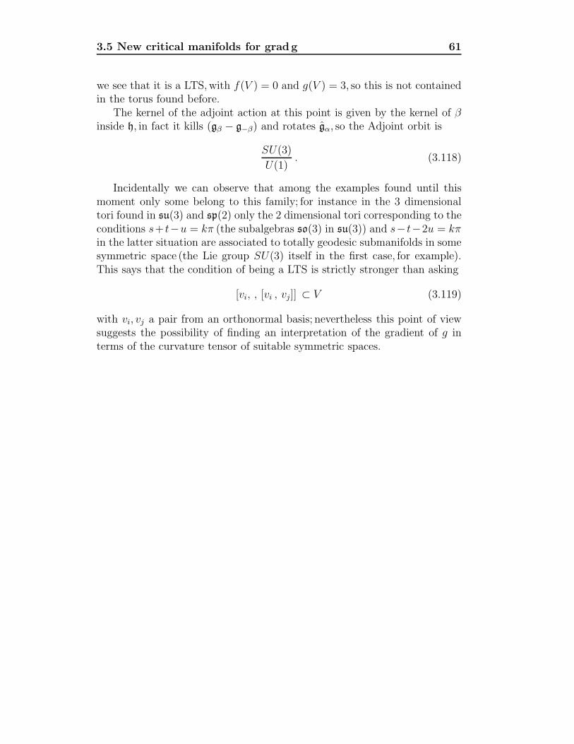
3.5 New critical manifolds for gradg 61
we see that it is a LTS,with f(V ) = 0 and g(V ) = 3, so this is not containedin the torus found before.
The kernel of the adjoint action at this point is given by the kernel of βinside h, in fact it kills (gβ − g−β) and rotates gα, so the Adjoint orbit is
SU(3)
U(1). (3.118)
Incidentally we can observe that among the examples found until thismoment only some belong to this family; for instance in the 3 dimensionaltori found in su(3) and sp(2) only the 2 dimensional tori corresponding to theconditions s+ t−u = kπ (the subalgebras so(3) in su(3)) and s− t−2u = kπin the latter situation are associated to totally geodesic submanifolds in somesymmetric space (the Lie group SU(3) itself in the first case, for example).This says that the condition of being a LTS is strictly stronger than asking
[vi, , [vi , vj]] ⊂ V (3.119)
with vi, vj a pair from an orthonormal basis; nevertheless this point of viewsuggests the possibility of finding an interpretation of the gradient of g interms of the curvature tensor of suitable symmetric spaces.

Chapter 4
Quaterion-Kahler spaces
In this chapter we introduce Quaternion-Kahler geometry, showing the mainexamples in the case of positive scalar curvature: compact Wolf spaces. Togive a more rich picture of the background we describe then the twistor andSwann bundles of Wolf spaces, which are important tools in the study ofquaternionic geometry, but which houwever will not play a crucial role in ourexposition. In Section 4.3 we introduce a way of describing the Sp(n)Sp(1)structure which is compatible with the tangent space of G3 at critical pointsfor f in a purely algebraic way: this is the first link between quaternionicand Grassmannian geometry. In this same spirit, in the last section we give anon-standard description of the Sp(2)Sp(1)-invariant 4-form in R8.
4.1 The Wolf Spaces
We state here the basic definitions and facts about Quaternion-Kaaler man-ifolds.References for this material are [71], [13], [44].
A Quaternion-Kahler manifold (from now on QK manifold) M of dimes-nion 4n is a Riemannian manifold characterized by the reduction of the re-stricted holonomy group Hol0 to the group Sp(1)Sp(n) ⊂ SO(4n); the com-plexified holonomy representation corrsponds to C2 ⊗ C2n ∼= H ⊗ E, whereH,E are the standard representations of Sp(1) and Sp(n) respectively.
The invariant symplectic 2-forms ωH , ωE can be used to describe the(symmetric) metric tensor in terms
g = ωH ⊗ ωE . (4.1)
These two representations have both a quaternionic structure, in other wordsan invariant antilinear endomorphism ε such that ε2 = −1; this structureallows to identify C2 with H and C2n with Hn. The tensor product εHE = εH⊗
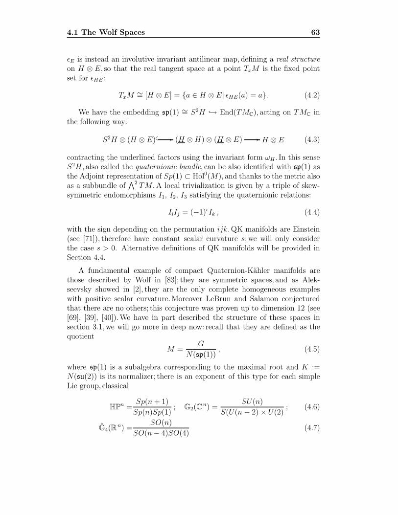
4.1 The Wolf Spaces 63
εE is instead an involutive invariant antilinear map, defining a real structureon H ⊗ E, so that the real tangent space at a point TxM is the fixed pointset for εHE :
TxM ∼= [H ⊗E] = a ∈ H ⊗ E| εHE(a) = a. (4.2)
We have the embedding sp(1) ∼= S2H → End(TMC), acting on TMC inthe following way:
S2H ⊗ (H ⊗ E) (H ⊗H) ⊗ (H ⊗E) H ⊗ E (4.3)
contracting the underlined factors using the invariant form ωH . In this senseS2H , also called the quaternionic bundle, can be also identified with sp(1) asthe Adjoint representation of Sp(1) ⊂ Hol0(M), and thanks to the metric alsoas a subbundle of
∧2 TM . A local trivialization is given by a triple of skew-symmetric endomorphisms I1, I2, I3 satisfying the quaternionic relations:
IiIj = (−1)εIk , (4.4)
with the sign depending on the permutation ijk. QK manifolds are Einstein(see [71]), therefore have constant scalar curvature s; we will only considerthe case s > 0. Alternative definitions of QK manifolds will be provided inSection 4.4.
A fundamental example of compact Quaternion-Kahler manifolds arethose described by Wolf in [83]; they are symmetric spaces, and as Alek-seevsky showed in [2], they are the only complete homogeneous exampleswith positive scalar curvature.Moreover LeBrun and Salamon conjecturedthat there are no others; this conjecture was proven up to dimension 12 (see[69], [39], [40]).We have in part described the structure of these spaces insection 3.1, we will go more in deep now: recall that they are defined as thequotient
M =G
N(sp(1)), (4.5)
where sp(1) is a subalgebra corresponding to the maximal root and K :=N(su(2)) is its normalizer; there is an exponent of this type for each simpleLie group, classical
HPn =Sp(n+ 1)
Sp(n)Sp(1); G2(C
n) =SU(n)
S(U(n− 2) × U(2); (4.6)
G4(Rn) =
SO(n)
SO(n− 4)SO(4)(4.7)

4.2 The Twistor space 64
and exceptional:
G2
SO(4);
F4
Sp(3)Sp(1);
E6
SU(6)Sp(1); (4.8)
E7
Spin(12)Sp(1);
E8
E7Sp(1). (4.9)
These spaces are all symmetric and have positive scalar curvature; their non-compact duals give examples of QK symmetric spaces of negative scalarcurvature; the theory of negative QK manifolds has rather different devel-opments with respect to the positive case: for instance Alekseevsky foundexamples which are homogeneous but non-symmetric ([3]). However we willfocus our attention exclusively on the positive case.
Going back to our examples, the tangent space at the point at eK can beidentified with m in the Lie algebra decomposition
g = c ⊕ sp(1) ⊕ m (4.10)
where c denotes the centralizer of sp(1) so that K is the adjoint group tothe subalgebra c ⊕ sp(1); so K is the stabilizer of a point and the holonomygroup of M via the Adjont action on m; the structure of a QK manifold isgiven by a field of algebras of skew-symmetric endomorphisms of the tangentspce isomorphic to Im H: in this case these algebras correspond to the sp(1)of the previous decomposition; in fact sp(1) acts on m by adjoint represen-tation (restricting the brackets of g) and in this way we have a K-invariantimmersion
sp(1) m ⊗ m
(where the duality m ∼= m∗ is provided by the Killing metric, which inducesthe G invariant Riemannian metric on M); K-invariance allows to extendedthe action of sp(1) globally on the whole M as a subbundle of End(TM).
4.2 The Twistor space
We want to discuss now some important homogeneous spaces which arebundles over the Wolf spaces; they can be generalized to bundles over anyQuaternion-Kahler manifold, as was shown by Salamon ([71]). Consider thecomplexification of any compact semisimple Lie algebra gC; let h be a Cartansubalgebra, and
gC = h ⊕∑α∈Ξ
gα (4.11)

4.2 The Twistor space 65
the correspondin Cartan decomposition,with gα the root spaces of the rootssystem Ξ; then g is a maximal compact subalgebra of gC, and [h] denotes theintersection h ∩ g; let ρ denote the highest root and consider the parabolicsubalgebra of gC
p = h ⊕∑
〈α,ρ〉≥0
gα ; (4.12)
then if P ⊂ GC denotes the corresponding adjoint subgroup,we can definethe complex homogeneous space of complex dimension n
Z =GC
P; (4.13)
we observe that p is precisely the subalgebra of the stabilizers of the complexline Cgρ, so Z can be interpreted as the GC orit under the adjoint action ofthe point Cgρ in the projectivised Lie algebra P(gC); instead the orbit of anynilpotent element Xρ ∈ gρ inside gC is given by
U =GC
P1, (4.14)
where P1 is the adjoint group of the Lie algebra p1 defined as
p1 := a ∈ p|〈a,Hρ〉 = 0, (4.15)
because the semisimple element Hρ doesn’t stabilize Xρ; in particular we havethe quotient p/p1
∼= C, so the projection
U =GC
P1
−→ GC
P= Z (4.16)
gives a bundle with fibre exp C = C∗; this bundle can be considered as thepricnipal bundle of a complex line bundle over the base space Z. The tangentspace at the identity of U can be identified with
TeP1U = Hρ ⊕∑
〈α,ρ〉<0
gα ; (4.17)
we can define on it an Ad(P1)-invariant cotangent vector
Y −→ 〈Xρ, Y 〉 (4.18)
which thus extends globally to a GC-invariant holomorphic 1-form θ; it canbe shown that θ satisfies
1. (dθ)n+1 = 0 ;

4.2 The Twistor space 66
2. the restriction of θ to the fibre is identically 0 ;
3. τ ∗z θ = zθ if τz is the action of C∗ on U .
We are going now to define a type of structures which are strictly relatedto the homogeneous spaces we are discussing:
Definition 4.1. Let C be a complex manifold of dimension 2n+1; a complexcontact structure is a family (Ui, θi) where the Ui is an open covering ofC and the θi are 1-forms defined on each Ui such that (dθi)
n ∧ θi = 0 in Ui
and θj = fijθi with fij some smooth function defined on Uj ∩ Ui;moreoverit’s required that this family is the maximal enjoying these properties.
The functions f−1ij can be viewed as transition functions for a comples line
bundle over C, which thus turns out to be naturally associated to the contactstructure; its principal bundle π : B −→ C with fibre C∗ can be equippedwith a global 1-form obtained gluing together the pullbacks π∗θi. On the otherhand, given a principal C∗ bundle B over a complex manifold C, the presenceof a holomorphic 1-form satisfiying conditions 1, 2, 3 above descends on Cto a complex contact structure.Applying these facts to our examples, we cansay that Z is a complex manifold endowed with a complex contact structuregiven by the holomorphic 1-form θ defined on the principal bundle U .
Now the compact subgroup G ⊂ GC acts on Z, giving rise to a compactorbit through eP which can be described as
M ′ =G
G ∩ P ; (4.19)
the subalgebra of the stabilizer is given by
g ∩ p = g ∩ (h ⊕∑
〈α,ρ〉=0
(gα + g−α))
(4.20)
as g doesn’t intersect a single root space gα; the following lemma shows thatactually the G orbit has the same dimension of the ambient space, so that inconclusion M ′ = Z and this last is compact:
Lemma 4.1. The following equality holds:
dimR GC − dimR G = dimR P − dimR G ∩ P (4.21)
Proof. The summand on the left side equals 12
dimRGC; on the right sidewe can subdivide in two parts: the Cartan subalgebra and the root spacesinvolved.Clearly dimR h = 2

4.2 The Twistor space 67
dimR h∩g; regarding the root spaces involved in p we can divide them in twotypes: those for which 〈α, ρ〉 > 0 and those for which 〈α, ρ〉 = 0;we observethat all positive roots satisfy one of these conditions (p is parabolic!). In thefirst case if gα ⊂ p then g−α ⊂ p, and
dimR
∑〈α,ρ〉>0
gα =1
2dimR
∑〈α,ρ〉=0
gα ; (4.22)
in the second case g±α ⊂ p and
dimR
∑〈α,ρ〉=0
(gα + gα) = 2 dimR
⎛⎝g ∩∑
〈α,ρ〉=0
(gα + gα)
⎞⎠ . (4.23)
The conclusion follows.
Hence, denoting l = p∩g and L the corresponding subgroup,we can writein compact presentation
Z =GC
P∼= G
L. (4.24)
We note now thatl = c ⊕ iHρ ⊂ N(sp(1)) , (4.25)
so we have again a fibrationZ −→M , (4.26)
with fibre the quotientSp(1)
U(1)∼= S2 , (4.27)
whose tangent space at the identity in Z is given by
g ∩ (gρ + g−ρ) . (4.28)
The following theorem, due to Wolf ([83],Th.6.1), states more precisely therelationship between contact and quaternionic structures in the homogeneouscontext:
Theorem 4.2. There is a one-to-one correspondence between compact sim-ply connected homogeneous contact complex manifolds Z and compact QKsymmetric spaces M . This correspondence is given by a bundle π : Z −→Mwith fibres 2-spheres.

4.3 The Sp(1)Sp(n) structure 68
The following diagram syntethizes the relationships between the variousspaces involved in the previous description:
GC/P1 ∼=
U
C∗
gC
G/L ∼=
GC/P ∼=
Z
S2
P(gC)
G/N(su(2)) ∼= M
G3
. (4.29)
Example.The main example to consider is quaternionic projective space:
Hn+1\0 CP2n+1 HPn (4.30)
Observation.The twistor bundle Z is non-trivial in general, and for compactQK manifolds with s > 0 it does not admit any global integrable section (see[70], [7]), or in other words any global complex structure compatible withthe quaternionic structure; in the case of HPn Massey proved in [63] thatno global almost complex structure exists at all. In the case of the complexGrassmannians G2(C
n), it is well known that they carry a global complexstructure J ; in the case J belongs to (S2H)⊥ inside End(TM), so that it isnot a section of Z.
4.3 The Sp(1)Sp(n) structure
Let h, h denote a unitary basis of H , in such a way that ωH(h, h) = 1;withrespect to this basis we have
ωH = h ∧ h =1
2(hh− hh) . (4.31)
We can in terms of h, h dtermine a basis of S2H :
I1 = ı(h ∨ h)
I2 = h2 + h2 (4.32)
I3 = ı(h2 − h2)
are orthogonal of norm√
2 with respect to the metric ωH ⊗ ωH induced onS2H ; they satisfy the same relations of quaternions:
I2k = −1 , IiIj = sgn(ijk)Ik (4.33)

4.3 The Sp(1)Sp(n) structure 69
with sgn(ijk) the sign of the permutation; the composition is obtained bycontracting again with ωH just as in (4.3).
Consider now the case where the Sp(1) representation inside Sp(1)Sp(n)is such that the projection on the Sp(n) factor is nonzero: this means thatthe E representation is nontrivial under this Sp(1) action.
In this case it becomes significant analyzing the quaternionic action fromthe point of view of these new Sp(1) representations; first of all we adopt thefollowing notation:we have the symmetrization map S acting on tensors as
S(x1 ⊗ · · · ⊗ xn) =1
n!
∑πn
xπn(1) ⊗ · · · ⊗ xπn(n) (4.34)
where π varies in the group of permutations on n elements; the map extendslinearly. We give then the following definition:we denote as
·, · : Σk ⊗ Σh Σh+k (4.35)
the symmetrization of the two factors,more explicitly if
α =∑πk
απk(1) ⊗ · · · ⊗ απk(k) ∈ Σk , β =∑πh
βπh(1) ⊗ · · · ⊗ βπh(h) ∈ Σh
(4.36)then
α⊗ β =∑πk,πh
S(απk(1) ⊗ · · · ⊗ απk(k) ⊗ βπh(1) ⊗ · · · ⊗ βπh(h)
). (4.37)
In particular we denote by σ the map ·, · when the first index is 2:
σ := ·, · : Σ2 ⊗ Σi Σi+2 . (4.38)
Consider now for simplicity the case that E corresponds to an irreducibleSp(1) representation; then
TxMC∼= Σ1 ⊗ Σi−1 (4.39)
and using Clebsch-Gordan relation,we obtain
TxMC∼= Σi + Σi−2 Σi+2 + Σi + Σi−2 ∼= Σ2 ⊗ Σi ; (4.40)
more precisely TxMC coincides with the kernel of the symmetrization
σ : Σ2 ⊗ Σi → Σi+2 . (4.41)

4.3 The Sp(1)Sp(n) structure 70
Example 4.1. There are essentially three ways (up to conjugation) of send-ing Sp(1) inside Sp(2): two correspond to the roots, but in these cases thedecomposition of the standard Sp(2) representation C4 is not irreducible; infact
E = C4 = Σ0 + Σ0 + Σ1 (4.42)
for the long root, as comparing with the known decomposition of the adjointrepresentation one has
sp(2) = S2(C4) = S2(2Σ0 + Σ1) = Σ2 + 2Σ1 + 3Σ0 ; (4.43)
for the short root we have instead
E = C4 = Σ1 + Σ1 (4.44)
as in factsp(2) = S2(C4) = S2(2Σ1) = 3Σ2 + Σ0 . (4.45)
There is a third embedding, corresponding to the sl(2,C) triple
X =
⎛⎜⎜⎝0
√3 0 0
0 0 0√
20 0 0 0
0 0 −√3 0
⎞⎟⎟⎠ , Y =
⎛⎜⎜⎝0 0 0 0√3 0 0 0
0 0 0 −√3
0√
2 0 0
⎞⎟⎟⎠ , (4.46)
H =
⎛⎜⎜⎝3 0 0 00 1 0 00 0 −3 00 0 0 −1
⎞⎟⎟⎠ , (4.47)
obtained using the recipe in [21], for which
E = C4 = Σ3 . (4.48)
Observation.This last can be interpreted in the following way: recall thatthe decomposition of the Lie algebra g2 with respect to so(4) ⊂ g2 is givenby
Σ2+ + Σ2
− + Σ1− ⊗ Σ3
+ , (4.49)
where Σk± denote the representations of the sp(1) corresponding to the long
(+) or to the short(−) root; so considering the diagonal embedding
sp(1)∆ so(4) = sp(1)+ + sp(1)−
sp(1)+ + sp(2) , (4.50)
consistently with the Sp(1)Sp(2) structure of the Wolf space
G2
SO(4), (4.51)

4.3 The Sp(1)Sp(n) structure 71
we have a description of its tangent space in the EH formalism as H ⊗E ∼=Σ1 ⊗ Σ3, corresponding to the representation in (4.48).
The action of S2H ∼= Σ2 on TxMC can be therefore expressed suit-ably exploiting this new formulation, involving the Σ2 factor instead of theΣ1 = H ; to understand more deeply this Σ2-approach we need to define moreexplicitly the invariant immersion (4.40). Let us define the map as
Q : Σ1 ⊗ Σi−1ωH⊗ Σ1 ⊗ Σ1 ⊗ Σ1 ⊗ Σi−1 ·,· Σ2 ⊗ Σi (4.52)
acting in the following way: if
Y = h⊗ β + h⊗ β ∈ Σ1 ⊗ Σi−1, β, β ∈ Σi−1 (4.53)
then
Q(Y ) =1
2hhhβ +
1
4(hh + hh)
(hβ − hβ)− 1
2hhhβ (4.54)
obtained, after tensorizing with the invariant element ωH , by symmetrizationof the tensorial factors respecting the simple or double underlining marks in(4.52).
Our next aim is to express the quaternionic action in terms of this de-scription: a first guess in this sense is that for Q(Y ) =
∑vi ⊗ pi then
Q(I1Y ) = v2 ⊗ p3 + v3 ⊗ p2 , (4.55)
mimicking the adjoint representation of su(2) on itself; but this is not cor-rct, as at the second step
Q(I21Y ) = −v2 ⊗ p2 − v3 ⊗ p3 , (4.56)
which is not −Id. Something more is needed to “reconstruct” the missingterm −v1 ⊗ p1.
The next proposition gives the correct answer in order to express thequaternionic action from the Σ2 viewpoint:
Proposition 4.3. Let Y ∈ TxM = Σ1 ⊗ Σi; if Q(Y ) =∑vi ⊗ pi then
Q(I1Y ) = v1 ⊗ 14σ(Y ) + v2 ⊗ p3 − v3 ⊗ p2 . (4.57)

4.3 The Sp(1)Sp(n) structure 72
Proof.We have the definition of Q(Y ) as in (4.54): then if we identify vi
with the basis Ii defined in (4.32), grouping the terms properly we obtain
p1 = − ı
4
(hβ − hβ) (4.58)
p2 =1
4
(hβ − hβ) (4.59)
p3 = − ı
4
(hβ + hβ) ; (4.60)
the quaternionic action of I1 on Y is given, in the Σ1 context, by
I1Y = −ıh⊗ β + ıh⊗ β ; (4.61)
so we obtain
Q(I1Y ) = − ı
2hhhβ +
ı
4(hh+ hh)
(hβ + hβ
)− ı
2hhhβ (4.62)
and in the form Q(I1Y ) =∑3
i=1 vi ⊗ q1i we have
q11 =
ı
4
(hβ + hβ) (4.63)
q12 = − i
4
(hβ + hβ) (4.64)
q13 = −1
4
(hβ − hβ) ; (4.65)
the conclusion follows by the definition of σ and comparing the two sets ofequalities.
In the same way we obtain for the other quaternionic elements
I2Y = −h⊗ β + h⊗ β (4.66)
I3Y = ıh⊗ β + ıh⊗ β (4.67)
so that
Q(I2Y ) = 12hhhβ − 1
2hh(hβ + hβ
)+ 1
2hhhβ (4.68)
Q(I3Y ) = ı2hhhβ + ı
2hh(hβ − hβ
)− ı2hhhβ (4.69)
which imply the equalities
qij = ηijk pk − δj
i
1
4σ(Y ) , (4.70)
where ηijk = sgnijk if i = j, otherwise ηiik = 0;moreover
pi = −1
4σ(IiY ) . (4.71)

4.4 The quaternionic 4-form in 8 dimensions 73
We can therefore state the quaternionic relations in terms of this descrip-tion: for example
Q(I21Y ) = Q(I1I1Y ) = −v1 ⊗ 1
4σ(I1Y ) − v2 ⊗ p2 − v3 ⊗ p3 (4.72)
= −v1 ⊗ p1 − v2 ⊗ p2 − v3 ⊗ p3 (4.73)
= −Q(Y ) (4.74)
and also
Q(I1I2Y ) = −v1 ⊗ 1
4σ(I
2Y ) − v2 ⊗ q2
3 − v3 ⊗ q22 (4.75)
= −v1 ⊗ p2 + v2 ⊗ p1 − v3 ⊗ 1
4σ(Y ) (4.76)
= Q(I3Y ) (4.77)
as expected.
4.4 The quaternionic 4-form in 8 dimensions
The local triple of almost complex structures Ii generate together with themetric a local triple of symplectic forms
ωi ∈2∧TxM , (4.78)
spanning a subbundle of the bundle of 2-forms isomorphic to S2H . The con-dition Hol0(M) ⊂ Sp(1)Sp(n) can be expressed by the condition that thesubbundle S2H is preserved by covariant differentiation,more precisely
∇Y ω1 = α3(Y )ω2 + α2(Y )ω3
∇Y ω2 = −α3(Y )ω1 + α1(Y )ω3 (4.79)
∇Y ω3 = α2(Y )ω1 − α1(Y )ω2 ;
where αi are local 1-forms and Y is any tangent vector.We can define a global4-form using these local 2-forms:
1
2Ω = ω1 ∧ ω1 + ω2 ∧ ω2 + ω3 ∧ ω3 (4.80)
and the following conditions are equivalent:
∇Y S2H ⊂ S2H ⇐⇒ ∇Y Ω = 0 (4.81)

4.4 The quaternionic 4-form in 8 dimensions 74
for any Y ∈ TxM . Swann proved in [78] that if dim M ≥ 12 then the condi-tion ∇Y Ω = 0 is equivalent to
dΩ = 0 ; (4.82)
Salamon showed an example of an 8-demensional compact nilmanifold en-dowed with 4-form Ω with stabilizer Sp(2)Sp(1), which is closed but non-parallel ([74]).
We want now to give a description of the quaternionic 4-form Ω using thepoint of view of the previous section: suppose for example that we have as in(4.48)
TxMC∼= Σ1 ⊗ Σ3 ∼= Σ2 ⊕ Σ4 ; (4.83)
then the bundle S2H can be detected finding the Σ2 summands in∧2 TxM :
2∧TMx
∼=2∧
Σ2 ⊕ Σ2 ⊗ Σ4 ⊕2∧
Σ4 (4.84)
∼= Σ2
v⊕ (Σ6 ⊕ Σ4 ⊕ Σ2)
m
⊕ (Σ6 ⊕ Σ2)h
; (4.85)
the elements of the three groups of summands will be called vertical,mixedand horizontal.We fix a basis of the vertical space to be e23, e31, e12, withrespect to a basis e1, e2, e3 of the Σ2 summand in (4.83); a basis of the Σ4
component of the tangent space is given by
e8 =1√3(2 · 11 − 22 − 33) (4.86)
e7 = (22 − 33) (4.87)
e4 = (12 + 21) (4.88)
e6 = (23 + 32) (4.89)
e5 = (31 + 13) , (4.90)
where the notation “11” stands for e1⊗e1, underlining in this way the identity
Σ4 ∼= S20 Σ2 . (4.91)
We want now to identify a basis for the horizontal part; the copy of Σ2 con-tained in
∧2 Σ3 is also a submodule of End(Σ4) and its elements can bedescribed in terms of invariant operations, as the following example shows:
β1(e4) = β1(12+21) = (1∗1)∨2+(1∗2)∨1 = 0+3∨1 = (31+13) = e5 , (4.92)

4.4 The quaternionic 4-form in 8 dimensions 75
where ∗ is the isomorphism∧2 Σ2 ∼= Σ2 and ∨ is symmetrization; this de-
scription is unique up to a constant, thanks to Schur’s lemma an the presenceof a unique copy of Σ2 in End(Σ4). Going on in the same way we obtain:
β1(e6) = β1(23 + 32) = (1 ∗ 2) ∨ 3 + (1 ∗ 3) ∨ 2 = 2(33 − 22) = −2e7 ;
(4.93)
β1(e5) = β1(31 + 13) = (1 ∗ 3) ∨ 1 + 0 = −(21 + 12) = −e4 ; (4.94)
β1(e7) = β1(22 − 33) = (1 ∗ 2) ∨ 2 − (1 ∗ 3) ∨ 3 = 2(32 + 23) = 2e6 ; (4.95)
β1(e8) = β1(1√3(2 · 11 − 22 − 33)) =
1√3(0 − (1 ∗ 2) ∨ 2 − (1 ∗ 3) ∨ 3)
(4.96)
= −(32 + 23) + (23 + 32) = 0 . (4.97)
Analogous calculations determine the following basis of the horizontal 2-forms
β1 = − 2e76 − e45 (4.98)
β2 =√
3e85 + e75 + e46 (4.99)
β3 = e74 −√
3e84 + e65 . (4.100)
Now the elements of the basis of the quaternionic bundle S2H ⊂ ∧2(S2 +S4) are decomposed as
ωi = ωhi + ωm
i + ωvi (4.101)
with
ωhi = βi (4.102)
ωmi =
8∑j=4
〈ei , ej〉 (4.103)
ωvi = ejk , (4.104)
where 〈 , 〉 denotes the contraction of tensors.We are going now to determinethe mixed term in the same spirit of what we did to find the βi, in other wordsfindig an invariant submodule in Σ2 ⊗Σ4 isomorphic to Σ2; subsequently wewill find constants a, b, c such that 〈ωi, ωi >= −I, if ωi = aωh
i + b ωmi + c ωv
i .

4.4 The quaternionic 4-form in 8 dimensions 76
Proposition 4.4. In this setting the quaternionic 4-form Ω is
1
2Ω = ω1 ∧ ω1 + ω2 ∧ ω2 + ω3 ∧ ω3
= −√
3e7653 − 2e7623 − e7681 −√
3e7642
− e4523 − 2e4581 +√
3e8142 +√
3e8153
+ e3175 − e8275 − e8246 + e7241
+ e6341 + e6385 − e7483 + e6512 .
Proof.We subdivide the proof in 3 parts:
1)The 2-form ω1.Starting with ωm
1 we have
ωm1 = 〈1 , 1√
3(2 · 11 − 22 − 33) + (22 − 33) (4.105)
+ (12 + 21) + (23 + 32) + (31 + 13)〉 (4.106)
=2√3e81 + 0 + e42 + 0 + e53 (4.107)
so that in total
ω1 = a(−2e76 − e45)h
+ b(2√3e81 + e42 + e53)
m
+ c(e23)v
, (4.108)
for some constants a, b, c; now we calculate 〈ω1 , ω1〉:
〈ω1 , ω1〉 = 〈a(−2e76 − e45) + b(2√3e81 + e42 + e53) + c(e23)
, a(−2e76 − e45) + b(2√3e81 + e42 + e53) + c(e23)〉
that more explicitely becomes
(−2a(76 − 67) − a(45 − 54)+
2√3b(81 − 18) + b(42 − 24) + b(53 − 35) + c(23 − 32))2
and contracting we obtain
− 4a2(77 + 66) − a2(55 + 44) − 4
3b2(11 + 88) − b2(44 + 22) − b2(55 + 33)
− c2(22 + 33) + ab(52 + 25) − bc(25 + 52) − ab(43 + 34) + bc(43 + 34)

4.4 The quaternionic 4-form in 8 dimensions 77
where the last four summands cancel each other if a = c.Moreover if weimpose the conditions
4a2 =4
3b2 = a2 + b2
the remaining terms have equal norms; in particular if we choose a = 12
and
b =√
32
) we obtain(ω1)
2 = −I .2)The 2-form ω2.We can do the same calculation for ω2: first of all we have
ωm2 = − 1√
3e82 + e72 + e63 + e41
so that
ω2 = a(√
3e85 + e75 + e46) + b(− 1√3e82 + e72 + e63 + e41) + c(e31)
or more explicitly
ω2 =c(31 − 13) − b√3(82 − 28) + b(72 − 27) + b(63 − 36)
+b(41 − 14) + a√
3(85 − 58) + a(75 − 57) + a(46 − 64) ,
so that squaring and contracting we obtain
〈ω2 , ω2〉 = − c2(33 + 11) − b2
3(88 + 22) − b2(77 + 22) − b2(66 + 33)
− b2(44 + 11) − 3a2(88 + 55) − a2(77 + 55) − a2(44 + 66)
− bc(34 + 43) + bc(16 + 61) +b2√3(87 + 78) + ab(25 + 52)
− ab(25 + 52) + ba(34 + 43) − ab(16 + 61) − a2√
3(87 + 78) ,
and if we impose the conditions seen for ω1, i.e. a = c = 12
and b =√
32
wehave
〈ω2 , ω2〉 = −I.
3)The 2-form ω3
In the same manner we obtain for ω3
ωm3 = − 1√
3e83 − e73 + e62 + e51

4.4 The quaternionic 4-form in 8 dimensions 78
so that
ω3 = a(e74 −√
3e84 + e65) + b(− 1√3e83 − e73 + e62 + e51) + c(e12)
= a(74 − 47) − a√
3(84 − 48) + a(65 − 56) − b√3(83 − 38)
− b(73 − 37) + b(62 − 26) + b(51 − 15) + c(12 − 21) ;
again contracting:
〈ω3 , ω3〉 = −a2(77 + 44) − 3a2(88 + 44) − a2(66 + 55) − b2
3(88 + 33)
− b2(77 + 33) − b2(66 + 22) − b2(55 + 11) − c2(11 + 22)
+ a2√
3(78 + 87) + ab(43 + 34) − ab(43 + 34) − ab(52 + 25)
+ ab(61 + 16) − b2√3(87 + 78) − bc(61 + 16) + bc(52 + 25)
and as usual for a = c = 12
and b =√
32
we obtain
〈ω3 , ω3〉 = −I .
Collecting together what we have found we obtain the 4-form Ω in terms ofthe chosen basis.

Chapter 5
Moment mappings andrealizations
In this Chapter we recall basic facts about QK moment maps, showing inthe simple case of a compact simple Lie group G acting transitively on aWolf space G/K how µ can be used to relate QK geometry to Grassman-nians. Then we discuss some well-known theory coming from Nilpotent or-bits, with results due to Kronheimer about the existence of HyperKaler met-rics on them; then an account of results is given from Swann’s theory,which isfor many aspects the most natural background for our approach.After thatwe present the description of an explicit trajectory for the flow of grad fin the case of so(4), together with the proportionality of grad f and grad galong it. This is used in the last two sections in order to describe explicitlythe realizations of some classical Wolf spaces in G3(g), for g the Lie algebraof a non-transitive group of isometries (in particular of cohomogeneity 1).
5.1 The moment mapping
Let G be a compact group acting on a differentiable manifold M preservingsome structure present on it, as for example a symplectic structure; then it ispossible to define a moment map
µ : M g∗ (5.1)
which under suitable hypotheses turns out to be G-equivariant, with respectto the Adjoint action of G on g. The main use of moment maps is thatof operating reductions, which means considering a fibre of µ, which is G-invariant, and then considering the quotient space under the G action: thisnew manifold M ′ inherits the structure of the first manifold M , offering a

5.1 The moment mapping 80
systemathic way of obtaining new examples of symplectic manifolds (see[33]).
This procedure has been generalized to other contexts: the Hyperkahlercase ([42]) and the QK case ([29] and [30]) for instance; the latter is the caseof our interest. The main difference in the QK case is that µ turns out to bea section
µ ∈ Γ(g ⊗ S2H) (5.2)
instead of a function; therefore only the zero-locus is well defined.
Observation.We point out that the moment map in the QK setting is au-tomathically equivariant.
In [29] Galicki and Lawson proved that µ is the only section of g ⊗ S2Hsatisfying
∇〈µ, A〉 =∑
(IiA) ⊗ Ii, (5.3)
where A ∈ g, A is the corresponding Killing vector field, Ii is the local basisof the bundle S2H and is the duality isomorphism of TM and T ∗M inducedby the metric.Moerover µ satisfies
µA := 〈µ, A〉 = c πS2H(∇(A)) (5.4)
where πS2H is the projection on the quaternionic bundle, seen as a subbundleof∧2 T ∗M , and c is a constant depending on the scalar curvature.As QK
manifolds are Einstein, then the scalar curveture s is constant, therefore wewill consider c = 1 for simplicity; we observe that the 2-tensor ∇A is skew-symmetric (see [55]).
In this context, Battaglia studied in [10], [11] the case where G = S1 usingMorse-theorethic methods, obtaining ([11])
Theorem 5.1. The complex Grassmannian G2(Cn) is the only positive QK
manifoldthat can be obtained as a QK quotient by a circle action.
We will make a rather different use of the QK moment map µ: in factwe will consider Lie groups G of arbitrary dimension, but with the aim ofobtaining immersions of a QK manifold in the Grassmannian G3(g); this ispossible because in local coordinates we have
µ =
3∑i=1
ωi ⊗Ai (5.5)
where ωi are a local orthonormal basis for S2H and Ai belong to g; if theAi are linearly independent, they span a 3-dimensional subdpace V ⊂ g

5.1 The moment mapping 81
which is independent from the trivialization, as the structure group for S2His SO(3). This determines a map
Ψ : M G3(g) (5.6)
which is defined only at the points x ∈ M for which Ai(x) are indepen-dent; therefore our hope is that the zero locus of µ is as small as possible.Aswe shall see in the examples discussed in Sections 5.4 and 5.5, the zero lo-cus will be empty, so no reduction would be possible at all in the cases wediscuss. In this sense we have (see [80, Proposition 3.5]).
Proposition 5.2. The set M0 is an open dense subset of the union⋃S of
G orbits on M such that dimS ≥ 3.
In this section we will exemplify our viewpoint obtaining the realizationof the classical Wolf spaces G/K in G3(g), using the moment map inducedby the action of the transitive group G. Let us denote by g the lie algebra ofG and let us consider the symmetric decomposition
g = k ⊕ m (5.7)
with k the Lie algebra of K = N(Sp(1)). The quaternionic subalgebra sp(1)corresponds to a 3 dimensional space of Killing vector fields on M whichvanish at the point eK; let us choose an orthonormal basis A1, A2, A3 whichcorrespond to Killing vector fields Ii; a well known result from the theory ofsymmetric spaces (see [13]) states that the covariant derivative of a Kvf Xcan be expressed at a point in the following way:
∇Y X|eK = [X, Y ]m , (5.8)
where Y ∈ m: from what we said before, the projection πS2H applied to the2-form 〈[X , ·] , ·〉 ∈ ∧2 m acts as the identity. In the case of the action of theisometry group G on the Wolf space M , we can ask ourselves what are thethree vis at a given point; in other words we are trying to solve the equation
πS2H(∇X) =3∑
i=1
〈vi , X〉ωi (5.9)
in the vis for any X ∈ g; now we observe that ωi = 〈[Ai , ·] , ·〉, and thanks toequation (5.8), putting X = Ai the (5.9) becomes
〈[Ai , ·] , ·〉 =
3∑i=1
〈vi , Ai〉〈[Ai , ·] , ·〉 ; (5.10)

5.2 Nilpotent orbits and Swann’s theory 82
on the other hand choosing X ∈ m the covariant derivative ∇X vanishes ateK, so equation (5.9) becomes
0 =3∑
i=1
〈vi , X〉〈[Ai , ·] , ·〉 (5.11)
and analogously if we choose X ∈ c the left hand side vanishes when weproject on S2H . In conclusion it must be
vi = Ai i = 1...3 . (5.12)
In conclusion we can deduce the following result:
Proposition 5.3. Let M be a Wolf space of the form G/K, with G a simpleLie group; let µ be the corresponding moment map and Ψ the induced mapwith values in G3(g); then Ψ embeds M in G3(g) and Ψ(M) is precisely thecritical manifold for the flow of grad f corresponding to the absolute maxi-mum.
5.2 Nilpotent orbits and Swann’s theory
Let g∗C
denote a complex simple Lie coalgebra; the orbit OX of any elementX under the coadjoint action of GC is naturally endowed with the Kirillov-Kostant-Soriau complex nondegenerate holomorphic 2-form ω, acting at thepoint X in the following way:
ωX(AY , AZ) = 〈X, [Y, Z]〉 (5.13)
on tangent vectors AY , AZ obtained by infinitesimal action of Y, Z ∈ gC ;because of the duality induced by the Killing form we can refer to the Liealgebra g in place of the coalgebra.The presence of such complex symplecticstructure is typical of HyperKahler manifolds, where ω = ωJ + ıωK is holo-morphic with respect to the first complex structure I. It is therfore natural toask if exists any metric on O making it a HK manifold in such a way that theinduced complex symplectic structure is just the one in (5.13).Kronheimershowed in [58] the existence of such metrics on orbits of nilpotent elementsidentifying them whit the moduli spaces of the solutions of a system of ODEcalled Nahm equations (see also [24]); the proof is based on Hitchin’s workabout HyperKaler metrics on moduli spaces ([41]).
Let us now describe briefly how Nahm equations arise: in the space ofconnections on a vector bundle V over a manifold M , those which are critical

5.2 Nilpotent orbits and Swann’s theory 83
points of the Yang-Mills functional
YM(∇) =1
2
∫M
Tr(F ∧ ∗F ) (5.14)
are called instantons, and have importance in particle physics (∗ is the Hodgeoperator of the metric on M and F is the curvature 2-form of the connection∇). Equivalently, the curvature form F of such critical points satisfies the(anti)-self-dual equations
F = ± ∗ F . (5.15)
Consider now the 4-dimensional Euclidean space R4 = S3 ×R; the Lie groupSU(2) is topologically S3 and its Lie algebra su(2) can be identified with afamily of left invariant vector fields globally trivializing the tangent bundleTS3, with a basis given by e1, e2, e3; consider now the trivial principal G bun-dle P = (S3 × R) × G for some compact Lie group G; then any linear mapL(t) : su(2) → g, depending on time t ∈ R, determines a global g-valued1-form, that is a connection form on a trivial G-bundle over S3 × R,SU(2)-invariant under its left multiplication. It is always possible to find a gaugetransform for which the connection takes the form
dt+ α1A1 + α2A2 + α3A3 , (5.16)
with αi ∈ su(2)∗ satisfying dαi = 2εijα1 ∧ αj and Ai ∈ g.Consider now the Chern-Simons functional φ : g × g × g → R defined as
φ(A1, A2, A3) =3∑
i=1
〈Ai, Ai〉 + 〈A1, [A2, A3]〉 (5.17)
whose gradient flow equations A = −gradφ are just the Nahm equationsquoted above:
A1 = −2A1 − [A2, A3]
A2 = −2A2 − [A3, A1] (5.18)
A3 = −2A3 − [A1, A2] ;
these equations are equivalent to the anti-self-duality condition (5.15) for theconnection identified by a map L defined as
L(e1) = Ai , i = 1, · · · , 3 ; (5.19)
in other words each trajectory for the gradient field gradφ in g × g × grepresents an instanton for the trivial bundle discussed above.

5.2 Nilpotent orbits and Swann’s theory 84
Critical points for gradφ turn out to be Lie algebra homomorphismsL : su(2) → g: the functional φ is strictly related to the functional f onG3(g); compare in fact (5.18) with the gradient of f (3.1).
The link with the nilpotent orbits is obtained complexifying equations(5.18) and passing from su(2) subalgebras in g to sl(2,C) subalgebras in gC.
Nilpotent orbits
Nilpotent orbits in a complex semisimple Lie algebra have been completelyclassified (see [21]). The nilpotent variety N ⊂ gC consisting of all the nilpo-tent elements in the algebra is an algebraic variety; the orbits O have a partialordering described by the relation
O1 < O2 ⇔ O2 ⊃ O1 ; (5.20)
the element 0 gives the only 0-dimensional orbit, contained in the closure ofall other ones. Just above of this in the ordering we have the minimal nilpo-tent orbit Omin, the one generated by a nilpotent element Xρ in a highestroot space gρ; going one step more up we find the next-to-minimal orbits. Atthe other extreme of the diagram we find the principal orbit Oprinc, the one ofmaximal dimension,which is an open subset of N . Nilpotent orbits are in cor-respondence with three dimensional Lie subalgebras, isomorphic to sl(2,C)and presented in standard form as a triple Y,H,X, withX, Y nilpotent andH semisimple; Jacobson-Morozov theorem states partly this correspondence:
Theorem 5.4. Let gC be a complex semisimple Lie algebra. if X is a nonzeronilpotent element of g, then there exists a standard triple for g whose nilpos-itive element is X.
Actually the correspondence is bijective, as two standard triple having incommon a nilpotent element X are in the same AdGC
orbit, and analogouslyif they share the same semisimple element H (see [21] and [57]).Moreover,semisimple elements have the special property of satisfying
〈H,α〉 ∈ 0, 1, 2 (5.21)
for any α simple root; thus we can identify the triple, up to conjugacy, by justlabelling every node of the Dynkyn diagram with 0, 1 or 2, obtaining a socalled weighted Dynkin diagram (wDd).
Observation.In this way we obtain at most 3rank g possible choices, provingthat nilpotent orbits are finite in number;we note that for semisimple orbitsthe situation is much different: fo example semisimple orbits in sl(2,C) are

5.2 Nilpotent orbits and Swann’s theory 85
0 Omin Oprinc
Figure 5.1: Hasse diagram for sl(3)
AdGCφ : sl(2,C) → g
OX
1:1
1:1 wDd
OH
(5.22)
Figure 5.2: Nilpotent orbits,3-dimensional Lie subalgebras and weightedDynkin diagrams.
parametrized by C/Z2. However this upper bound is rather rough, not all3rank g are attached to any standard triples: for example in Table 5.1 is shownthe Hasse diagram for sl(3), with 3 orbits, whereas 3rank sl(3) = 32 = 9.
We have thus a correspondence between nilpotent orbits, conjugacy clas-ses of 3-dimensional subalgebras and weighted Dinkyn diagrams (see Figure5.2). In the case of classical Lie algebras, nilpotent orbits can be identifiedby a partition: for example for sl(n) nilpotent orbits are in bijective corre-spondence with the partitions of n; in this way the minimal nilpotent orbithas associate partition: 2, 1, · · · , 1︸ ︷︷ ︸
n−2
, also denoted by [2, 1n−2]. For the other
classical algebras, sp(n) and so(n), which are subalgebras of sl(N) for N bigenough, nilpotent orbits are in bijective correspondence with appropriate sub-sets of all the partitions of N .
Unstable manifolds in G3
Wolf spaces can be identified with maximal critical submanifolds of the Grass-mannian G3(g) for the flow of grad f , as we have seen in Chapter 3; on theother hand their Swann bundle U appears as the minimal nilpotent orbitOmin in the complexified algebra gC;U has a HyperKaler structure ([79])and Kronheimer’s results extend this property to any nilpotent orbit. It istherefore natural to ask if any of them fibres over a QK manifold,with fibreH∗/Z2. Swann prooved that this is in fact the case: nilpotent orbits always
5.2 Nilpotent orbits and Swann’s theory 86
admit an action of H∗, so that O/H∗ is a QK manifold.The quotient manifold can be identified again with a submanifold of the
Grassmannian G3(g) using the functional f , but in general, for orbits whichare not minimal, it is not merely a critical submanifold for grad f (whichoften has the wrong dimension), but an unstable submanifold connecting twocritical sets, one of which contains the copy of su(2) corresponding to anynilpotent element X ∈ O (see the Jacobson-Morosov theorem above). Let usrecall the main results in this sense: consider the Chern-Simons functionalφ, together with a map L as seen in (5.19) which defines a critical point (andhence an su(2) representation in g); let OL be the nilpotent orbit associatedto L(su(2)) (the orbit of a nilpotent element in L(su(2))C); then we have ([80,Theorem 4.1 b), c) ]):
Theorem 5.5. Let L : su(2) → g be a critical point for the functional φand let ML denote the set of φ trajectories A(t) such that limt→∞A(t) = 0and limt→−∞A(t) is in the same Adjoint orbit of L(su(2)); then ML admitsa free action of H∗/Z2 and the quotient ML is a QK manifold;moreover forany standard C∗ ⊂ H∗, the quotient ML/C∗ is isomorphic both to P(OL) andto the twistor space ZL of ML.
The link between the Chern-Simons functional φ and the functional fdiscussed in Chapter 3 is contained in the next result ([80, Theorem 5.2]:
Theorem 5.6. Let OL be a nilpotent orbit, and let ML be its H∗ quotient; thenML is isomorphic to the f unstable submanifold M ′
L of G3(g) associated tothe critical set containing L(su(2)).
Let us denote by Z ′L the twistor space of M ′
L; then the isomorphisms justdiscussed are expressed by
ZL
∼= Z ′L
∼=
P(OL)
∼=
. (5.23)
What QK manifolds can be obtained starting from a nilpotent orbit? Thenext result provides, using a moment map construction in the complex con-tact setting, an answer to this question:
Theorem 5.7. Let M be a QK manifold whose isometry group is com-pact; suppose that its twistor space Z is homogeneous with respect to a sub-group C of the complexified group GC. Then M is locally isometric to ML,

5.3 A trajectory for so(4) 87
where OL is the nilpotent orbit in gC obtained in Theorem 5.5; in particu-lar M has positive scalar curvature. Conversely, every nilpotent orbit in gC
gives rise to a QK manifold of positive scalar curvature, with twistor spacehomogeneous under GC.
Observation.The QK structure is reconstructed using the Inverse TwistorConstruction ([59]).
Consider now the complexification VC of a 3-dimensional space V ∈G3, then the isotropic cone C is defined by equation
x2 + y2 + z2 = 0 (5.24)
with respect to an orthonormal basis e1, e2, e3 of V ; let us denote by F ⊂ G3
the subset of 3-planes such that C consists of nilpotent elements; then wehave (see [80, Section 3])
Proposition 5.8. If Z has an open GC orbit then Ψ(M) ⊂ F .
Here the map Ψ : M → G3(g) is that induced by the QK moment map asdiscussed in Section 5.1; this property will be significant in Chapter 6,wherethe existence of an open GC orbit on Z will be considered a basic hypothesis.
5.3 A trajectory for so(4)
In this section we study in more detail the example of g = so(4).We wish tothank A.F. Swann for taking to our attention the importance of this example([77]).
We introduce for so(4) = su(2)+⊕su(2)− the following way of representing3 dimensional subspaces: let e1, e2, e3 and f1, f2, f3 be orthonormal basesof the subalgebras su(2)+ and su(2)− respectively; then a subspace V notintersecting the su(2)− subalgebra can be described through an element X ∈Hom(su(2)+, su(2)−) so that a basis is given by ei + Xei; with this notationthe space V can be identified in Λ3so(4) by
γ =(e1 + Xe1) ∧ (e2 + Xe2) ∧ (e3 + Xe3) (5.25)
= e1 ∧ e2 ∧ e3 + S(e1 ∧Xe2 ∧Xe3)
+S(Xe1 ∧ e2 ∧ e3) + Xe1 ∧ Xe2 ∧ Xe3 ,
whose norm is given by
‖γ‖2 = 1 + S|Xe1 ∧ Xe2|2 + S|Xe1|2 + |Xe1 ∧ Xe2 ∧ Xe3|2= det(I + XXT ) = cXXT
(−1)
5.3 A trajectory for so(4) 88
(with the last expression we mean the “total Chern class” of the matrix XXT
in a formal sense); in this way, as f is linear on Λ3so(4) and as it is nonzeroonly in the e123 and f123 directions, it can be expressed in function of X as
f(X) = f(e123)〈 γ
‖γ‖ , e123〉 + f(f123)〈 γ
‖γ‖ , f123〉 (5.26)
=
√2(1 + det(X))
(det(I + XXT ))12
. (5.27)
Now if we suppose that X is an invertible matrix, defining X = det(X)X−1,we can differentiate and calculate grad f using this alternative description:
d
dtf(X + tY ) =
d
dt
√2(1 + det(X + tY ))
(det(I + (X + tY )(X + tY )T ))12
(5.28)
and considering the case where A = I + XXT is invertible one has
d
dt(det(I + (X + tY )(X + tY )T )) =
d
dtdet(I + XXT
+t(XY T + YXT ) + t2(Y Y T ))
= Tr(A (XY T + YXT )) ,
and on the other hand
d
dtdet(X + tY ) = Tr(XY ) ; (5.29)
so putting everything together we obtain
grad f |X(Y ) =
√2
cXXT (−1)
(Tr(XY ) (cXXT
(−1))12 +
− (1 + detX)Tr(A (XY T + YXT ))
2(cXXT (−1))12
);
moreover as Tr(BC) = Tr(CB) for any matrices B and C and as A is sym-metric, we can write
grad f |X =
√2
cXXT (−1)
((cXXT
(−1))12 X− 1 + detX
(cXXT (−1))12
AXT
)(5.30)
acting on tangent vectors by the inner product defined by Tr(grad f · Y ); inparticular for X = I we obtain the diagonal subalgebra su(2)∆, where it’s

5.3 A trajectory for so(4) 89
immediate to check that grad f = 0 as we well know.Now we can differentiateagain around this point to obtain an analogous expression for the hessian. Infact using the same arguments we obtain the following expression of Hess fas a quadratic form:
Hess f |X=I(Y ) =cY2 (−1) − c
(Y T +Y2
)
2 (−1) − Tr(Y Y T
2) + 1
2(Tr(Y ))2
2; (5.31)
now it’s immediate to check that the decomposition of the 9 dimensionaltangent space in su(2) modules corresponds to the following type of matrices:
Σ0 = spanI (5.32)
Σ2 = Λ3R3 (5.33)
Σ4 = S20(R
3) . (5.34)
Observation.If we consider X belonging to SO(3) we see that f is con-stant; as the critical set M at X = I is isomorphic to RP3 we can in this wayidentify it with SO(3), and the tangent space is just so(3) = Λ3R3.
We start now to move in the Σ0 direction, along the curve
X(t) = t I , t ≥ 0 ; (5.35)
we notice that V (X(0)) = su(2)+,V (x(1)) = su(2)∆ and limt→∞ V (X(t)) =su(2)−; so we obtain
f(X(t)) =
√2 (1 + t3)
(1 + t2)32
(5.36)
and
grad f(X(t)) =
√2 (−1 + t) t
(1 + t2)52
I ; (5.37)
so this is an integral curve of the flow of grad f but with the wrong parame-trization.Orthonormal bases of V (X(t)) and of V ⊥(X(t)) are given by
ei + tfi√1 + t2
i=1...3
and
fi − tei√
1 + t2
i=1...3
; (5.38)
moreover X(t) = I, which represents the homomorphism snding ei + tfi tofi, whose projection on V ⊥ is given by⟨
fi ,fi − tei√
1 + t2
⟩fi − tei√
1 + t2=
(1√
1 + t2
)fi − tei√
1 + t2(5.39)

5.3 A trajectory for so(4) 90
1 2 3 4 5t
3.5
4
4.5
5
5.5
6
gXt
Figure 5.3: The graph of g(X(t))
so that as an element of V ⊗V ⊥, with respect to the given orthonormal basis,
X(t) =1
1 + t2I ; (5.40)
so with respect to this basis we obtain
grad f(X(t)) =
√2 (−1 + t) t
(1 + t2)32
I . (5.41)
Now recall thatg = 3f 2 + ‖grad f‖2 (5.42)
we get
g(X(t)) =6 (1 + t4)
(1 + t2)2 (5.43)
and one can check that the only critical points are just at t = 0 and t = 1(see Figure 5.3); this proves that grad g cannot be 0 on the other orbits met byX(t); but as the SO(4) action on the unstable manifold is of cohomogeneityone, this means that the behaviour of both f and g and essentially of everyAd invariant function h on the Grassmannian (in the sense of their valuesand gradients) on this submanifold can be completely reconstructed fromjust one trajectory, just because
dAdg(gradh|x) = gradh|gx ∀g ∈ SO(4) .
In other words g cannot have any other critical point on the whole unstablemanifold M∆ of f ,moreover grad g cannot be orthogonal to grad f on it, as

5.3 A trajectory for so(4) 91
the AdSO(4) action preserves the scalar product.All this mechanism holdsin general for any G simple group, so if we know 〈grad f , grad g〉 on onetrajectory emanting from this kind of critical manifold, that means that it lieson the f unstable Quaternionic-Kahler submanifold M(O) corresponding toa next-to-minimal nilpotent orbit O (see [22]), then we know it on the wholesubmanifold. In particular we have the following
Proposition 5.9. The unstable manifolds emanating from the critical setC∆ ⊂ G3(so(4)) for the flows of grad f and grad g are the same:
Mf∆ = Mg
∆ . (5.44)
Proof.Recall the usual way of representing the gradients of f and g andcompare them on the trajectory X(t): we have[
ei + tfi√1 + t2
,ej + tfj√
1 + t2
]=
[ei, ej] + t2[fi, fj]
1 + t2
and recalling that
[ei, ej] = ±√
2ek and [fi, fj] = ±√
2fk
(the sign depending on the parity of the permutation ijk), we can go oncalculating the j-th components of the gradients; so
−grad gj
2=
[ei + tfi√
1 + t2,[ei, ej] + t2[fi, fj]
1 + t2
]⊥+
[ek + tfk√
1 + t2,[ek, ej] + t2[fk, fj]
1 + t2
]⊥=
([ei, [ei, ej ]] + t3[fi, [fi, fj]]
(1 + t2)32
)⊥
+
([ek, [ek, ej]] + t3[fk, [fk, fj]]
(1 + t2)32
)⊥
= −4
(ej + t3fj
(1 + t2)32
)⊥
= −4
⟨ej + t3fj
(1 + t2)32
,fj − tej√
1 + t2
⟩fj − tej√
1 + t2
= 4
(t− t3
(1 + t2)2
)fj − tej√
1 + t2
and as we have seen
grad fj =√
2
(t2 − t
(1 + t2)32
)fj − tej√
1 + t2. (5.45)
Then we have
grad g = 4√
2
(1 + t√1 + t2
)grad f (5.46)

5.4 Realizations in cohomogeneity 1: HPn 92
M G M G
HPn Sp(n) G4(Rn) SO(n− 1)
HPn SU(n + 1) G4(R7) G2
HPn∏
i Sp(ki) G2/SO(4) SU(3)
G2(Cn) SU(n− 1) F4/Sp(3)Sp(1) Spin(9)
G2(C2n) Sp(n) E6/SU(6)Sp(1) F4
Table 5.1: Cohomogeneity 1 actions of semisimple Lie Goups on compactQK manifolds
on X(t) and in consequence on all M∆; hence the conclusion.Observation.This example is fundamental for us in the sense that so(4) canbe found as a subalgebra in many other Lie algebras g, so that equivariancearguments can help to generalize what is known in this case to the ambientalgebras. This will be exploited in the next Sections in order to identify theimage of the map Ψ in G3(g).Kobak and Swann used the abundance of copiesof so(4) to find Hyperkhaler potential on cohomogeneity 2 nilpotent orbits(see [52, Theorem 4.2]).
5.4 Realizations in cohomogeneity 1: HPn
We reprise the theme of Section 5.1 asking what happens if we apply the sameideas when a subgroup H of G acts on M : what is ΨH(M) for the inducedΨH? First we observe that in this case h ⊂ g and there is an inclusion
G3(h) G3(g) ; (5.47)
moreover because of the equivariance of ΨH theH orbit through eK is sent tothe intersection Ψ(M)∩G3(h). Before starting,we display in Table 5.1 a listof all cohomogeneity 1 actions on compact QK manifolds, see [22, Theorem7.4], for a detailed proof, and also [56] for a classification of cohomogeneity 1and hyperpolar actions.
In this section we will make use of some properties of rank one symmetricspaces; we collect the main results, taken from [35, Chap.VII,Prop.10.2 andTheor.10.3], in the following proposition.
Proposition 5.10. Let M be a compact Riemannian globally symmetricspace. Then M has a simply closed geodesic.If M is rank one, then all geo-desics are simply closed and have the same lenght.Moreover in this case, let

5.4 Realizations in cohomogeneity 1: HPn 93
2L denote the common lenght of the geodesics: if p is any point in M thenExp : TpM → M is a diffeomorphism of the open ball ‖X‖ < L in TpMonto the complement M − Ap, where Ap = Exp(‖X‖ = L) is called theantipodal set for p. This last, with the Riemannian structure induced by thatof M , is a Riemannian globally symmetric space of rank one, and a totallygeodesic submanifold of M .
We pass to a fundamental example.
SO(4) acting on HP(1)
The group SO(4) ⊂ Sp(2) is the stabilizer of a point in the standard presen-tation of the quaternionic projective space:
HP1 =Sp(2)
Sp(1)Sp(1);
we can fix a point (the class of e) and decompose the Lie algebra of Sp(2) asusual:
sp(2) = so(4) ⊕ m
where m = [E⊗H ] quaternionically; this means that if we decompose so(4) assu(2)+⊕su(2)− then E andH represent the standard complex representationsof the two summands (that extend globally to the Spin bundles).Now ifwe act on HP(1) by the action of elements g ∈ Sp(2) we get analogousdecompositions, so that at the point corresponding to the class of g we get
sp(2) = Adgso(4) ⊕ Adgm . (5.48)
We can now decompose elements of so(4) projecting them on the summandsof the new decomposition: so if X ∈ so(4) then
X = π1,gX + π2,gX (5.49)
where πi,g is the projection on the i-th summand in (5.48); we observe thatthe quaternionic structure at the point corresponding to g is provided byAdgsu(2)− by adjoint action on Adgm.We have a representation of so(4) onthe module TgSO(4)HP1 ∼= Adgm via the adjoint action, but the π2 compo-nent has no effect in consequence of the symmetric space structure; so theprojection on Adgso(4) is the significant part, and in particular the subspace
π−11,g (Adgsu(2)−) ∩ so(4) (5.50)
acts as ImH on Adgm; so it becomes interesting understanding (5.50) in or-der to explain the interaction between the action of the fixed SO(4) andquaternionic bundle.We have the following proposition:

5.4 Realizations in cohomogeneity 1: HPn 94
Proposition 5.11. Let Ψ be the map induced by te moment map µ of theaction of SO(4) on HP1 with values in G3(so(4)); then Ψ(HP1) = M∆ ∪su(2)+ ∪ su(2)−, where M∆ is the unstable manifold associated to the criticalmanifold containing su(2)∆; in particular:
Ψ(N) = su(2)− (5.51)
Ψ(S) = su(2)+ (5.52)
Ψ(γ(π/4)) = su(2)∆ . (5.53)
Proof:We choose now the following copy of U(1) ⊂ Sp(2):
g(t) =
⎛⎜⎜⎝cos t sin t 0 0− sin t cos t 0 0
0 0 cos t sin t0 0 − sin t cos t
⎞⎟⎟⎠ = exp
⎛⎜⎜⎝0 t 0 0−t 0 0 00 0 0 t0 0 −t 0
⎞⎟⎟⎠ , (5.54)
where the matrix on the right is denoted by t u. If we identify the northpole N of S4 ∼= HP1 with the class of e, this subgroup (we observe thatU(1) ⊂ SO(4)) moves along a geodesic γ(t) connecting N (t = 0) with thesouth pole S (t = π/2) passing through the equator (t = π/4), and thenbackwards to N (t = π). The curve obtained is a section with respect to theaction of SO(4), in fact it is obtained by exponentiation of a straight linepassing through the origin in the tangent space at the point N , which is thestandard representation of SO(4) on R4; the SO(4) equivariance of the mapExp implies that γ(t) is transverse to each orbit (the principal ones are copiesof S3 and the singular ones are N and S) and intersects all of them.Moreoverthe stabilizer of the SO(4) action is constant along the curve on points thatare different from N and S, and coincides with SO(3)∆, both along γ(t) inHP1 and along u(1) for the isotropy representation. So restricting to theinterval t ∈ (0, π/2), the nonvanishing Kvf are given by π2,gso(4) and somecalculations shows in fact that
π2,g(su(2)∆) ≡ 0 ;
on the contrary the only Kvf whose covariant derivative is nonzero at thepoints γ(t) are precisely π−1
1,g(Adgso(4)); in particular if X ∈ so(4) then
∇(·)X = [π1,g(t)X , · ] (5.55)
at the given point; but the only vectors whose induced antisymmetric en-domorphism is contained in the quaternionic algebra are those given by(5.50), as we already observed.

5.4 Realizations in cohomogeneity 1: HPn 95
Now we recall the notation used in section 5.3 to study the flow of grad fin so(4): ei and fi denote orthonormal bases of su(2)+ and su(2)− respec-tively; as so(4) is a subalgebra of sp(2) corresponding to the longest root, theelements of the two copies of su(2) correspond to the following matrices:
e1 =1√2
⎛⎜⎜⎝ı 0 0 00 0 0 00 0 −ı 00 0 0 0
⎞⎟⎟⎠ , f1 =1√2
⎛⎜⎜⎝0 0 0 00 ı 0 00 0 0 00 0 0 −ı
⎞⎟⎟⎠ , (5.56)
e2 =1√2
⎛⎜⎜⎝0 0 1 00 0 0 0−1 0 0 00 0 0 0
⎞⎟⎟⎠ , f2 =1√2
⎛⎜⎜⎝0 0 0 00 0 0 10 0 0 00 −1 0 0
⎞⎟⎟⎠ (5.57)
and
e3 =1√2
⎛⎜⎜⎝0 0 ı 00 0 0 0ı 0 0 00 0 0 0
⎞⎟⎟⎠ , f3 =1√2
⎛⎜⎜⎝0 0 0 00 0 0 ı0 0 0 00 ı 0 0
⎞⎟⎟⎠ ; (5.58)
so if ei(t) and fi(t) denote an orthonormal basis of Adg(t)so(4), we get via theKilling metric:
〈ei , fj(t)〉 = δij sin2 t (5.59)
〈ei , ej(t)〉 = δij cos2 t (5.60)
〈fi , ej(t)〉 = δij sin2 t (5.61)
〈fi , fj(t)〉 = δij cos2 t ; (5.62)
the conclusion is that at the point γ(t)
πg(t)su(2)− (ei) = sin2 t fi(t) , πg(t)su(2)− (fi) = cos2 t fi(t) , (5.63)
or in terms of Kvf
πS2H(∇ei) = sin2 t fi(t) , πS2H(∇fi) = cos2 t fi(t) (5.64)
and the moment map for the action of SO(4) on HP1 along γ(t) is given by
µ(γ(t)) =∑
i ωi ⊗ (cos2 t fi + sin2 t ei) , (5.65)

5.4 Realizations in cohomogeneity 1: HPn 96
up to a constant. This is the only information that we need to reconstructthe moment map on the whole HP1, as γ intersects all the orbits and themoment map is equivariant.
We can now interpret these facts in terms of the induced map Ψ: if we lookfor a moment to equation (5.65) and we go back to (5.35), we can see thatthe span of vi(t) consists exactly of the 3-planes V (t) along the trajectorythat generates the unstable manifold for grad f in G3(so(4)): the conclusionfollows.
Observation.The map Ψ is not injective. The points corresponding to t andπ − t are sent to the same 3-plane; so the principal orbits of type S3 in HP1
are sent to the orbits of type RP3 in M∆. The map Ψ becomes injective onthe orbifold HP1/Z2.
Generalizing to HPn
We go now to consider HPn under the action of Sp(n)Sp(1), the subgroup ofSp(n+ 1) which stabilizes a point, obtaining the following proposition whichextends 5.11:
Proposition 5.12. Let G = Sp(n)Sp(1) ⊂ Sp(n + 1) be the stabilizer ofa point N of HPn; then the map Ψ induced by the action of G with valuesin the Grassmannian G3(sp(n) ⊕ sp(1)−) sends HPn in M ′
∆ ∪ HP(n − 1) ∪su(2)−; the map Ψ is compatible with the standard inclusion of HP1 in HPn
as the following commutative diagram shows:
HPn Ψ1
2:1 G3(n, 1)
HP1Ψ2
2:1
G3(so(4)) ;
(5.66)
moreover we have the same equations as in Proposition 5.11, where S belongsto AN .
Proof. At a Lie algebra level we have the following decompositions:
sp(n + 1) = sp(n) ⊕ sp(1)− ⊕ n (5.67)
where n is as usual the quaternionic isotropy representation [E ⊗H ], of co-homogeneity one; then,also:
sp(n+ 1) = sp(n− 1) ⊕ sp(1)+ ⊕ n′ ⊕ sp(1)− ⊕ n ; (5.68)

5.4 Realizations in cohomogeneity 1: HPn 97
we added the subscripts +,− to distinguish the copies of sp(1), and also tobe consistent with the previous paragraph: in fact we can find a copy ofsp(2) ⊂ sp(n+ 1) such that
sp(2) ∩ (sp(n) ⊕ sp(1)−) = sp(1)+ ⊕ sp(1)− (5.69)
[sp(2) , sp(n− 1)] = 0 (5.70)
〈sp(2) , n′〉 = 0 , (5.71)
so that we can exploit the results for HP1: in fact the Lie algebra of theprincipal stabilizer of the isotropy representation is precisely sp(n − 1) ⊕su(2)∆, where su(2)∆ ⊂ sp(1)+⊕ sp(1)−, and if we take the element in (5.54)we obtain a geodesic as for HP1, with antipodal point for t = π/2; evolvingsp(n + 1) under adjoint action,we obtain the usual effect on the copy ofsp(2) obviously, and moreover sp(n − 1) is left fixed, because of condition(5.70); regarding n′, in view of (5.71) and as sp(2) is preserved by Adg(t), wecan conclude that it remains orthogonal to the latter under this action, sothat in particular 〈Adg(t)n
′ , sp(1)−〉 ≡ 0. So reasoning exactly as for HP1 wesee that the only Kvf along γ(t) with nonzero covariant derivative are thosegiven by sp(n− 1) ⊕ su(2)∆, but the projection on sp(1)− kills the elementsin sp(n− 1).
The conclusion is that the image in the Grassmannian G3(sp(n)⊕ sp(1))(from now on in this section denoted as G3(n, 1) for brevity) under the Ψinduced by the moment map of this action is given by the 3 planes obtainedin so(4) = sp(1)+ ⊕ sp(1)− under the inclusion
so(4) ⊂ sp(n) ⊕ sp(1)− ⊂ sp(n + 1) . (5.72)
Now consider the critical manifolds in G3(n, 1): as the algebra is not sim-ple, we get 2 absolute maxima, a point corresponding to sp(1)− and a copy ofHP(n − 1) corresponding to sp(n); another critical point is given by su(2)∆,included in so(4) as in (5.72); we describe the decomposition of the tangentspace of the Grassmannian at su(2)∆, in terms of the representations of thewhole stabilizer Sp(n− 1)SO(3)∆:
sp(n) ⊕ sp(1)− = sp(n− 1) ⊕ sp(1)+ ⊕ n′ ⊕ sp(1)−= [S2E ⊗ C] + [Σ2
∆] + [E ⊗H+] + [Σ2]
with E,H+ are the standard sp(n− 1) and sp(1)+ representations as usual,and the Σ2 is the antidiagonal representation in so(4); so, in terms of complexrepresentations,

5.4 Realizations in cohomogeneity 1: HPn 98
Tsu(2)∆G3(n, 1) = Σ2∆ ⊗ (E ⊗ Σ1 + S2E ⊗ Σ0 + Σ2
∆ + Σ2) (5.73)
= E ⊗ (Σ3 + Σ1) + S2E ⊗ Σ2 + (Σ4 + Σ2 + Σ0) (5.74)
so that the tangent space to the 4n− 1 dimensional critical manifold C∆ isgiven by
Tsu(2)∆C∆ = E ⊗ Σ1 + Σ2 (5.75)
and the unstable bundle by
W = Σ0 ; (5.76)
this implies that C∆ is a principal orbit too, in particular the Z2 quotient ofS4n−1, and moreover that the cohomogeneity of the unstable manifold M ′
∆ isone, as usual when the corresponding nilpotent orbit is next-to-minimal.
Remark. In fact if g1 and g2 are two simple Lie algebras,O1 and O2 theminimal nilpotent orbits of gi ⊗ C (of cohomogeneity 1 with respect to theG action), then
cohomG1G2O1 ×O2 = cohomG1O1 + cohomG2O2 = 2 (5.77)
and O1 ×O2 is next-to-minimal in the partial order for both minimal orbits(in fact contains them).
We have in conclusion the following commutative diagram of inclusions,thanks to the compatibility of grad f with the inclusion of subalgebras:
M ′∆
i G3(n, 1)
M∆
i
G3(so(4)) .
which implies the result.
Observations. 1)The antipodal set AN = Exp(S4n−1(π/2)) of the point Nis sent Sp(n)Sp(1)-equivariantly to HP(n− 1), and if we leave SO(4) actingon the tangent space we get an S3 ⊂ S4n−1 which is sent in the same pointby the exponential map; so we have the following composition of equivariantmaps:

5.5 Realizations in cohomogeneity 1: G2(C2n) and G4(R
n) 99
Ψ Exp : S4n−1 HP(n− 1) , (5.78)
whose fibre contains S3; then we have the following sequence of fibrations:
S4n−1 = Sp(n)Sp(1)Sp(n−1)SU(2)∆
Exp ANΨ Sp(n)Sp(1)
Sp(n−1)SO(4) ; (5.79)
for dimensional reasons we conclude that the antipodal set is precisely HP(n−1), a well known fact (see [19]).
2)It is tempting to restrict to the subgroup Sp(n) ⊂ Sp(n + 1); its actionis still of cohomogeneity 1 on HPn, so it a good candidate for an immersioncompatible with the next-to-minimal unstable manifolds.However lookingmore carefully we can see that in this case the moment map becomes
µ(γ(t)) =1
λ
∑i
ωi ⊗ sin2 t ei , (5.80)
so it degenerates at the point N ,moreover Ψ(γ(t)) for t = 0 is constantlysu(2)+, and the whole manifold is squashed onto the maximal critical HP(n−1) in G3(sp(n)); then there is no intersection of Ψ(HPn) with M∆, and in con-sequence no hope of using the dynamics of grad f to describe the quaternionicstructure.We will see in the next section that in this sense the action of Sp(n)will be more efficient on the complex Grassmannians.
3)The Z2 action on HPn is the one induced by the symmetry at the pointN . In this case M∆ is isomorphic to (see [80]):
HPn\(N ∪ HP(n− 1))
Z2. (5.81)
Remark. In Chapter 6 the conformality of Φ will be considered as a generalhypothesis; in the examples here in discussion the conformal factor is givenby the function
λ2(t) = sin4 t+ cos4 t , (5.82)
shown in figure 5.4.
5.5 Realizations in cohomogeneity 1: G2(C2n)
and G4(Rn)
We go now to discuss analogous immersions for complex Grassmannians,which are rank two symmetric spaces; this implies that we have no hope of
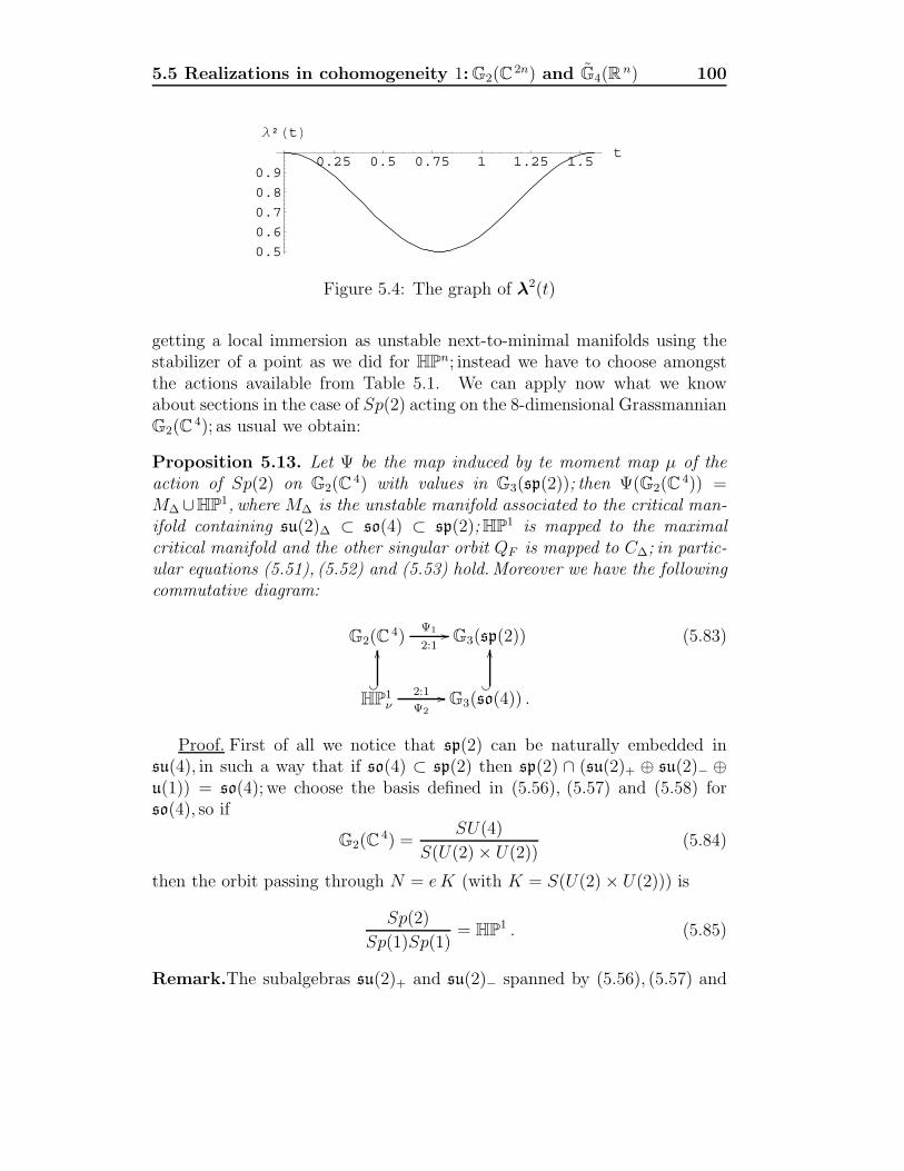
5.5 Realizations in cohomogeneity 1: G2(C2n) and G4(R
n) 100
0.25 0.5 0.75 1 1.25 1.5t
0.5
0.6
0.7
0.8
0.9
Λ²t
Figure 5.4: The graph of λ2(t)
getting a local immersion as unstable next-to-minimal manifolds using thestabilizer of a point as we did for HPn; instead we have to choose amongstthe actions available from Table 5.1. We can apply now what we knowabout sections in the case of Sp(2) acting on the 8-dimensional GrassmannianG2(C
4); as usual we obtain:
Proposition 5.13. Let Ψ be the map induced by te moment map µ of theaction of Sp(2) on G2(C
4) with values in G3(sp(2)); then Ψ(G2(C4)) =
M∆ ∪HP1, where M∆ is the unstable manifold associated to the critical man-ifold containing su(2)∆ ⊂ so(4) ⊂ sp(2);HP1 is mapped to the maximalcritical manifold and the other singular orbit QF is mapped to C∆; in partic-ular equations (5.51), (5.52) and (5.53) hold.Moreover we have the followingcommutative diagram:
G2(C4)
Ψ1
2:1 G3(sp(2))
HP1ν Ψ2
2:1
G3(so(4)) .
(5.83)
Proof. First of all we notice that sp(2) can be naturally embedded insu(4), in such a way that if so(4) ⊂ sp(2) then sp(2) ∩ (su(2)+ ⊕ su(2)− ⊕u(1)) = so(4); we choose the basis defined in (5.56), (5.57) and (5.58) forso(4), so if
G2(C4) =
SU(4)
S(U(2) × U(2))(5.84)
then the orbit passing through N = eK (with K = S(U(2) × U(2))) is
Sp(2)
Sp(1)Sp(1)= HP1 . (5.85)
Remark.The subalgebras su(2)+ and su(2)− spanned by (5.56), (5.57) and

5.5 Realizations in cohomogeneity 1: G2(C2n) and G4(R
n) 101
(5.58) are SU(4)-conjugate to copies of su(2) embedded respectively as(A 00 0
),
(0 00 B
)(5.86)
for A,B ∈ su(2), via the element⎛⎜⎜⎝−1 0 0 00 0 −1 00 −1 0 00 0 0 1
⎞⎟⎟⎠ ; (5.87)
thus both su(2)± correspond to the minimal nilpotent orbit also if we seethem inside su(4).
The slice representation νN is R4 with the standard SO(4) action, and isspanned by
k1 =
⎛⎜⎜⎝0 0 0 10 0 −1 00 1 0 0−1 0 0 0
⎞⎟⎟⎠ , k2 =
⎛⎜⎜⎝0 0 0 ı0 0 −ı 00 −ı 0 0ı 0 0 0
⎞⎟⎟⎠ (5.88)
and
k3 =
⎛⎜⎜⎝0 1 0 0−1 0 0 00 0 0 −10 0 1 0
⎞⎟⎟⎠ , k4 =
⎛⎜⎜⎝0 ı 0 0ı 0 0 00 0 0 ı0 0 ı 0
⎞⎟⎟⎠ ; (5.89)
we choose the geodesic β(t) identified by k4, that is
g(t) = exp(t k4) =
⎛⎜⎜⎝cos t ı sin t 0 0ı sin t cos t 0 0
0 0 cos t ı sin t0 0 ı sin t cos t
⎞⎟⎟⎠ ; (5.90)
clearly it is closed and orthogonal to HP1 at β(0),so it is a section. Followingthe evolution of the quaternionic structure and projecting on it the antysim-metric endomorphisms generated by sp(2) as we did before, we get an expres-sion for the moment map µ(β(t)) which is identical to (5.65).Recall that themaximal critical manifold for the flow of grad f in G3(sp(2)) is HP1;moreoverthe next-to-minimal critical manifold C∆ corresponds to the diagonal subal-gebra su(2)∆ ⊂ so(4), and at the level of nilpotent elements to the Jordan-type partition 22 (see [21] and [52]); the critical submanifold C∆ is the

5.5 Realizations in cohomogeneity 1: G2(C2n) and G4(R
n) 102
6-dimensional homogeneous manifold
Sp(2)
U(2)∆; (5.91)
this su(2)∆ is the one associated to the short root, and its centralizer is theu(1) corresponding to the matrix called u in (5.54).Now sp(2) decomposesin terms of SU(2) × U(1) representations as:
sp(2,C) = S2(Σ1 ⊗ (Am + A−m)) (5.92)
= Σ2 ⊗ (A2m + A−2m + Am ⊗ A−m) (5.93)
+ Σ0 ⊗ (Am ⊗ A−m) (5.94)
= Σ2 + Σ0 + Σ2 ⊗ (A2m + A−2m), (5.95)
where Am is some U(1) representation; the decomposition of the Grass-mannian’s tangent space at C∆ in terms of the whole isotropy group is:
Tsu(2)∆G3(sp(2)) = Σ2 ⊗ (Σ0 + Σ2 ⊗ (A2m + A−2m)) (5.96)
= Σ2 ⊕ (Σ4 + Σ2 + Σ0) ⊗ (A2m + A−2m) (5.97)
as we have seen in (3.102) in terms of SU(2) representations; the unstablebundle is
W = [Σ0 ⊗ (A2m + A−2m)] ∼= R2 (5.98)
which is of cohomogeneity 1 under the U(1) action.Looking more carefully, we can notice that
so(4) ⊕ νN∼= sp(2)ν , (5.99)
so we have two copies of sp(2) in su(4), satisfying
sp(2) ∩ sp(2)ν = so(4) ; (5.100)
geometrically this corresponds to the existence of another projective line,transversal to the first one and denoted by HP1
ν ; it is clear from the definitionsthat HP1
ν ⊃ β(t); the action of Sp(2) on it reduces to the well known actionof SO(4).As we saw previously, the spheres of ray 0 < r < π/2 in νN are mappeddiffeomorphically onto HP1
ν\N, S, while the sphere of ray π/2 is sent tothe single point S: so the differential of the exponential degenerates on it, andS belongs to a singular orbit. In G2(C
4) the first singular orbit correspondingto the points 0 is HP1 and su(2)∆ is the centralizer of k4 in the slicerepresentation, and as we pointed out before the differential dExp is regular

5.5 Realizations in cohomogeneity 1: G2(C2n) and G4(R
n) 103
for t < π/2; so the Kvf corresponfing to the antidiagonal representation inso(4) are preserved under it; in conclusion the 7-dimensional principal orbitshave type
Sp(2)
SU(2)∆; (5.101)
we notice that the evolution of the generator of the u(1)
k9 =
⎛⎜⎜⎝ı 0 0 00 −ı 0 00 0 ı 00 0 0 −ı
⎞⎟⎟⎠ , (5.102)
belonging to the algebra so(4)⊕ u(1) of the stabilizer on N , along β is givenby:
Adg(t)k9 =
⎛⎜⎜⎝ı cos 2t sin 2t 0 0− sin 2t −ı cos 2t 0 0
0 0 ı cos 2t sin 2t0 0 − sin 2t −ı cos 2t
⎞⎟⎟⎠ ; (5.103)
this belongs to sp(2) if and only if t = π/4 + k π/2 ; indeed for these valueswe get Adg(π/4)k9 = u and the orbit takes the form
QF =Sp(2)
U(2)∆
; (5.104)
where F stands for focal: in fact u ∈ sp(2) represents a Jacobi field whichvanishes at these values of the parameter; if N denotes the normal bundle ofHP1 and B ⊂ N is the sphere bundle of ray π/4 inside it, then QF is nothingelse than Exp(B), and u is the kernel of dExp there.Going on with the evolution we see that
Adg(π/2)(so(4) ⊕ u(1)) ∩ so(4) = so(4) ; (5.105)
so the second singular orbit (5.104) corresponds to 1 in the quotient space[0, 1], and at t = π/2 the geodesic β meets again HP1, but at a different point(su(2)+ and su(2)− are swapped); then it goes back to QF , and hence againto HP1, closing at t = π.In fact the points Ψ(β(π/4 + t)) and Ψ(β(π/4− t)) are on the same AdSp(2)-orbit in G3(sp(2)), more precisely
Ψ(β(π/4 + t)) = Adβ(π/2)Ψ(β(π/4 − t)) ; (5.106)

5.5 Realizations in cohomogeneity 1: G2(C2n) and G4(R
n) 104
the restriction of f to the trajectory Ψ(β(t)) is given by
f(Ψ(β(t))) =
√2(cos6 t+ sin6 t
)(cos4 t+ sin4 t
) 32
, (5.107)
with nonzero derivative in the interval (0, π/4), hence injective: so must be Ψwhen restricted to the union of orbits intersecting β in this interval.
Remark.HP1 and HP1ν are embedded isometrically, quaternionically and
(hence) totally geodesically in G2(C4).
Observations.1)This time we have a Z2 action corresponding to the isom-etry sending v in −v on the fibre of the normal bundle N of HP1; then wehave the following identification:
M∆∼= G2(C
4)\HP1
Z2. (5.108)
2)In [6] geodesics that are sections (called normal) are used to study coho-mogeneity 1 actions; there it is introduced the concept of the twist of suchgeodesics (which actually is independent of the chosen one), defined as:
tw(β) := |β ∩ P0| , (5.109)
where P0 is one of the singular orbits; in the case of G2(C4) with Sp(2) action
we have tw(β) = 2;moreover
tw(β) =1
2|W| (5.110)
(Theorem 6.1 in the cited paper), where W is the generalized Weyl Group,equal to N(β)/K, where N(β) is the subgroup preserving β globally and Kis the principal stabilizer, which preserves β pointwisely; in this case W is thedihedral group generated by reflections at the points β(0) and β(π/4), so itis isomorphic to Z2 ×Z2. Instead in the case of HP1 under the SO(4) actionwe had tw(γ) = 1 and W = Z2.
Generalizing to G2(C2n)
The inclusion sp(2) ⊂ sp(n) ⊂ su(2n) suggests how to generalize the previousresults to complex Grassmannians of dimension multiple of 8: in the samespirit of what we did with projective spaces, we have a decomposition
su(2n) = sp(n) ⊕ n (5.111)

5.5 Realizations in cohomogeneity 1: G2(C2n) and G4(R
n) 105
and both sp(2) and sp(2)ν can be immersed in sp(n) preserving the samerelations seen for G2(C
4); in particular if we evolve along exp(tk4), the de-composition
su(2n) = sp(2)ν ⊕ n′ (5.112)
is preserved, and as su(2)− ⊂ so(4) ⊂ sp(2)ν then the only elements whichhave nonzero projection on su(2)− are the same as for G2(C
4): in other wordswe obtain again the same expression for µ(β(t)) as in (5.65). The sp(n) orbitthrough exp(π/4 · k4) is again Exp(B) in the notation used before; this is theother singular orbit, which in this case is of type
QF =Sp(n)
Sp(n− 2) × U(2)∆
, (5.113)
so that again QF∼= C∆ up to a covering (see [22, Theorem 6.8]). Thus we
can extend Proposition 5.13:
Proposition 5.14. We have the exactly the same results as for Propostion(5.13), with the substitution of G2(C
4) with G2(C2n), sp(2) with sp(n),HP1
with HP(n− 1).
The Real Grassmannians G4(Rn)
We see from Table 5.1 that SO(n − 1) is the only group acting with co-homogeneity 1 on G4(R
n).We note the following low-dimensional isomor-phisms,which relate this case with the previous ones:
HP1 =Sp(2)
Sp(1)Sp(1)=SO(5)
SO(4)= S4 (5.114)
G2(C4) =
SU(4)
S(U(2) × U(2))=
SO(6)
SO(4) × SO(2)= G4(R
6) ; (5.115)
the second one suggest to translate what discussed in the previous subsectionfor G2(C
4) in terms of antisymmetric matrices; we obtain more in general:
Proposition 5.15. Let Ψ be the map induced by te moment map µ of the ac-tion of SO(n−1) on G4(R
n) with values in G3(so(n−1)); then Ψ(G4(Rn)) =
M∆ ∪ G4(Rn−1), where M∆ is the unstable manifold associated to the critical
manifold containing su(2)∆ ⊂ so(4) ⊂ so(n− 1); G4(Rn−1) is mapped to the
maximal critical manifold; in particular equations (5.51), (5.52) and (5.53)hold.Moreover we have the following commutative diagram:
G4(Rn)
Ψ1
2:1 G3(so(n− 1))
HP1ν Ψ2
2:1
G3(so(4)) .
(5.116)

5.5 Realizations in cohomogeneity 1: G2(C2n) and G4(R
n) 106
Proof.The following matrix explains pictorically the inclusions of su(3) ⊂so(4) and νN in so(6) ∼= su(4):⎛⎜⎜⎜⎜⎜⎜⎝
• • • 0 • • • 0 • • • 0 0 0 0 0 0 0 0 0 0
⎞⎟⎟⎟⎟⎟⎟⎠ (5.117)
where • represent elements in so(3), elements in so(4)\so(3), or in otherwords the antidiagonal elements, and finally the the slice representationνN . As observed before, so(4) ⊕ νN = sp(2)ν . Now the pattern is clear alsoin higher dimension: in fact so(4) and νN (which is always 4 dimensional)are embedded in the same way as in (5.117), just adding more columns androws of zeroes to the ones existing in this case. To exemplify the situa-tion,mantaining the notation used in the previous sections, we point out that:
k4 =
⎛⎜⎜⎜⎜⎜⎜⎝
0 0 0 0 . . . 00 0 0 0 . . . 00 0 0 0 . . . 00 0 0 0 . . . 2. . . . . . . . . . . . . . . . . .0 0 0 −2 . . . 0
⎞⎟⎟⎟⎟⎟⎟⎠ , e1 =1
2
⎛⎜⎜⎜⎜⎜⎜⎝
0 1 0 0 . . . 0−1 0 0 0 . . . 00 0 0 1 . . . 00 0 −1 0 . . . 0. . . . . . . . . . . . . . . . . .0 0 0 0 . . . 0
⎞⎟⎟⎟⎟⎟⎟⎠ .
We choose to evolve again along the geodsic β with β ′(0) = k4, the mostnatural thing to do to extend the 8 dimensional case; the form of the momentmap obatined is the usual one, exactly for the same arguments used before.In so(n) exist several next-to-minimal nilpotent orbits, and correspondinglyseveral next-to-minimal unstable manifolds, but the image of our Ψ resultsto be the one with related partition 3, 1n. Now the principal stabilizer isgiven by SO(3)∆ × SO(n− 5), and the 4n − 17 dimensional principal orbit(for n ≥ 6) is of type
SO(n− 1)
SO(n− 5) × SO(3)∆; (5.118)
this time all elements in so(n − 1) with nonzero entries at (4, 4 + h) forh = 1...n−5, represent a family of Jacobi fields which intersect the stabilizingsubalgebra so(4) × so(n − 4) along β with the same periodicity as u did inthe complex Grassmannians (see (5.103) and (5.104)), at t = π/4 + k π/2; inconsequence these values correspond again to the second singular orbit, whichhas form
Exp(B) = G3(Rn−1)F =
SO(n− 1)
SO(n− 4) × SO(3)∆, (5.119)

5.5 Realizations in cohomogeneity 1: G2(C2n) and G4(R
n) 107
which again coincides with C∆ up to a covering (see [22]); the conclusion isthe usual one.
Observations.1)Again we have a Z2 action sending v in −v in N , inducingthe equivariant diffeomorphism
M∆∼= G4(R
n)\G4(Rn−1)
Z2. (5.120)
2)Again we have tw(β) = 2 and W = Z2 × Z2.
Brylinski and Kostant classification
Something is missing in the previous sections. In fact Complex Grassman-nians of dimension 8n + 4 are not treated together with the other classicalWolf Spaces; we see from Table 5.1 that SU(n) is the only group acting withcohomogeneity 1 on these spaces, and if we try to perform the same typeof calculations as for other spaces on some low-dimensional example, we donot get the same type of answer: the image of Ψ seems not to be containedin the next-to-minimal unstable manifold as usual. This is not by chance: anexplanation for this phenomenon comes from Brylinski-Kostant classificationof shared nilpotent orbits: in fact in Table 5.2, taken from [49], but see also[15], we see that in the third column the algebra su(n) is missing (for n = 3); ifwe had a finite covering map from an open subset of G2(C
2n+1) to a next-to-minimal unstable manifold, then this would lift to a similar map at the levelof the Swann bundles, which are respectively minimal and next-to-minimalnilpotent orbits; then su(n) should appear in the table.

5.5 Realizations in cohomogeneity 1: G2(C2n) and G4(R
n) 108
Wolf Space(g′) g′ g k dim OG4(R
7) so(7) g2 1 8
G4(R2n+2) so(2n+ 2) so(2n+ 1) 2 4n− 2
G2(C2n) sl(2n) sp(2n) 2 4n− 2
E6/SU(6)Sp(1) e6 f4 2 22
G2/SO(4) g2 su(3) 3 6
G4(R2n+1) so(2n+ 1) so(2n) 2 4n− 4
F4/Sp(3)Sp(1) f4 so(9) 2 16
F4/Sp(3)Sp(1) f4 so(8) 4 16
G4(R8) so(8) g2 6 10
HPn−1 sp(n) ⊕k1sp(ni) 2k−1 2n
Table 5.2: Shared nilpotent orbits. The number k is the degree of the coveringO′ → O.

Chapter 6
Latent quaternionic geometry
In this final Chapter we describe in detail the quaternionic structure as itappears through the “Grassmannian filter”: the word “latent” expresses theidea that this strucure is in some sense already present in G3(g), but manifestitself only on the appropriate submanifolds.
6.1 The Coincidence Theorem
Suppose that the moment map µ induced by the action of a compact semi-simple Lie group G on M has the form
µ(x) =∑
i
Ii ⊗ Bi , (6.1)
where Bi = λ(x)vi, for vi an orthonormal basis of V = spanB1, B2, B3; inother words,µ induces a conformal map between the S2H bundle and therestriction of the tautological bundle V to Ψ(M); this hypothesis is not ex-cessively restrictive: in fact it was shown by Swann that if the twistor space Zhas an open GC orbit, then the image of µ is contained in the set F ⊂ G3 ofthoes 3-planes V such that the null cone of the complexification VC consistsof nilpotent elements (see Proposition 5.8); in this case
µC(I2 + ıI3) = B2 + ıB3 ∈ N ; (6.2)
but nilpotent elements in gC are isotropic with respect to the Killing form: infact thanks to Engel’s theorem their adjoint representation can be given interms of strictly upper triangular matrices, with respect to a suitable ba-sis, and the product of such matrices is still strictly upper triangular andhence traceless; in other words
0 = 〈B2 + ıB3 , B2 + ıB3〉 = ‖B1‖2 − ‖B2‖2 + 2ı〈B2 , B3〉 , (6.3)

6.1 The Coincidence Theorem 110
which implies B2 ⊥ B3 and ‖B2‖ = ‖B3‖, conditions that are equivalent toconformality.We assume along the whole section that this condition holdsfor the moment map µ.
Recall that µ satisfies the twistor equation
M
∇µA = s
3∑i=1
IiA ⊗ Ii , (6.4)
where A is the Killing vector field generated by A in g, means passing tothe corresponding 1-form via the metric and s is the scalar curvature, whichis constant as the metric is Einstein: for simplicity we can put s = 1.On theother hand on V we have defined the sections sA and the natural connectionG
∇ so that, as seen in Chapter 2,more precisely (2.19) and Proposition 2.3
G
∇sA =3∑
i=1
s⊥A ⊗ vi ⊗ vi . (6.5)
In general, given a differentiable embedding Ψ : M → N of manifolds, andan isomorphism Φ between vector bundles E → F on the manifold M and
N respectively, the second one equipped with a connectionF
∇ , we can define
the pullback connection Ψ∗ F
∇ acting in the following way on elements σ ofΓ(E):
(Ψ∗ F
∇)Y (σ) := Ψ−1(F
∇(Ψ∗Y )(Ψσ)) (6.6)
where Y ∈ TxM . In fact
Lemma 6.1. The operator Ψ∗ F
∇ defined on Γ(F ) is a connection.
Proof.We check that it satisfies the definition of a connection: it is clearlylinear in the Y , and as Φ is a homomorphism, for λ(x) a differentiable functionon M , we have
(Ψ∗ F
∇)Y (λσ) = Ψ−1(F
∇(Ψ∗Y )
(Ψλσ)
)(6.7)
= Ψ−1((Ψ∗Y )(λ)Ψσ + λ(
F
∇(Ψ∗Y )σ))
(6.8)
= Y (λ)σ + λΨ−1(F
∇(Ψ∗Y )σ)
(6.9)
= Y (λ)σ + λ(Ψ∗ F
∇)σ . (6.10)
6.1 The Coincidence Theorem 111
We want to apply this construction in our case, with the map Ψ : M →G3 induced by µ, N = G3, E = S2H, F = V, to prove the CoincidenceTheorem, which relates, at a fixed point x ∈M , the action of the quaternionicstructure on 1-forms induced by G (the duals of the Killing vector fields) withspecial cotangent vectors on the Grassmannian G3.
Before starting,we say in advance that the map Ψ : M → G3 can be liftedto an isomorphis between the quaternionic bundle S2H and the tautologicalbundle V; this question will be discussed in more detail in Section 6.2, butwe need it in the next proof in order to use the pullback connection.
Theorem 6.2. Let M, g,G3, µ be defined as usual, with
µ =
3∑i=1
Ii ⊗ Bi (6.11)
where Bi = λvi, λ a differentaiable G-invariant function on M and vi anorthonormal basis of a point V ∈ G3; let us choose A ∈ V ⊥ ⊂ g; then at thepoint x such that Ψ(x) = V , for Ψ induced by µ as usual, we have
1λIiA
= Ψ∗(A⊗ vi) , (6.12)
where A⊗ vi ∈ T ∗x G3.Moreover we have ‖µ‖2 = 3λ2.
Proof. Let Φ denote the conformal lift of the map µ so that
Φ(Ii) = Bi ; (6.13)
then
Φ(µA) = Φ
(3∑
i=1
Ii〈Bi , A〉)
= Φ
(λ
3∑i=1
Ii〈vi , A〉)
(6.14)
= λ3∑
i=1
Φ(Ii)〈vi , A〉 = λ23∑
i=1
vi〈vi , A〉 (6.15)
= λ2sA ; (6.16)

6.1 The Coincidence Theorem 112
then applying the Φ∗ G
∇ connection of S2H to µA we obtain
(Φ∗ G
∇)µA = Φ−1
(G
∇(Φ(µA))
)= Φ−1
(G
∇(λ2sA)
)(6.17)
=d(λ2)
λ2 µA + λ2Φ−1
(G
∇sA
)(6.18)
=d(λ2)
λ2 µA + λ2Φ−1
(3∑
i=1
s⊥A ⊗ vi ⊗ vi
)(6.19)
=d(λ2)
λ2 µA + λ
3∑i=1
Ψ∗(s⊥A ⊗ vi) ⊗ Ii ; (6.20)
on the other hand the difference of two connections on the same vector bundleis a tensor, so given any section σ ∈ S2H which vanishes at a point x ∈M
(M
∇− Ψ∗ G
∇)σ(x) = 0 ; (6.21)
but this is precisely the case for the section µA at the point x such thatΦ(S2Hx) = V , because A ∈ V ⊥ by hypothesis; in other words
M
∇µA |x = (Ψ∗ G
∇)µA |x ; (6.22)
thanks to the calculations in (6.17) and using the twistor equation (6.4), wecan deduce
3∑i=1
IiA ⊗ Ii = λ
3∑i=1
Ψ∗(s⊥A ⊗ vi) ⊗ Ii ; (6.23)
the result follows considering that s⊥A = A at V .
The Coincidence Theorem leads to various ways of relating elements inTxM ,TV G3 and the quaternionic elements Ii. In fact
Corollary 6.1. Let Y ∈ TxM such that
Ψ∗Y =∑
vi ⊗ Pi ; (6.24)
for Pi ∈ V ⊥ with V = Ψ(x); let us consider a tangent vector of the formX = (1/λ)
∑i IiPi in TxM ; then
X = Ψ∗((Ψ∗Y )). (6.25)

6.1 The Coincidence Theorem 113
Proof.Using the definitions and (6.12) we obtain
(Ψ∗Y )(Ψ∗Z
)= 〈∑
vi ⊗ Pi , Ψ∗Z〉G3 (6.26)
=1
λ〈∑
IiPi , Z〉M (6.27)
= X , (6.28)
for any Z ∈ TxM , hence the conclusion.Observation.We are using the homomorphism in two different mean-ings, depending on what metric we are considering: in one case that on TV G3
and in the other in TxM .
Another consequence of the Coincidence Theorem 6.2 is
Corollary 6.2. Under the hypotheses of Theorem 6.2 we have
Ψ∗I1X =1
λ
∑j
〈X , Aj〉M v1 ⊗ Aj (6.29)
− 1
λ
∑j
〈X , I3Aj〉M v2 ⊗ Aj
+1
λ
∑j
〈X , I2Aj〉M v3 ⊗Aj .
with 〈, 〉M the metric on M ; analogous statements are valid for I2, I3.
Proof.We have
Ψ∗X =∑i,j
〈Ψ∗X , vi ⊗Aj〉G3 vi ⊗ Aj (6.30)
=1
λ
∑i,j
〈X , IiAj〉M vi ⊗ Aj (6.31)
and applying one of the quaternionic endomorphisms we obtain immediately(6.29).Observation.We notice that the first summand in (6.29) does not dependon I1.
The equivariance of the moment map µ implies that Kvf on M are sentto Kvf on G3: in other words if A is induced by A ∈ g on M , then
Ψ∗A =
3∑i=1
vi ⊗ [A , vi]⊥ . (6.32)

6.1 The Coincidence Theorem 114
Let now α =∑3
i=1 vi ⊗ pi ∈ T ∗x G3 and let Ar be an orthonormal basis of
V ⊥; then
d−3∑r=1
〈Ψ∗α, Ar〉Ar =
d−3∑r=1
〈α, Ψ∗Ar〉Ar =∑i,r
〈pi, [vi , Ar]⊥〉Ar (6.33)
=∑i,r
〈 pi, [vi , Ar] 〉Ar =∑i,r
〈[pi, vi] , Ar〉Ar (6.34)
=∑
i
[pi, vi]⊥ . (6.35)
We can therefore define a mapping
ρ : T ∗xM V ⊥ (6.36)
by ρ(σ) =∑
r〈σ , Ar〉Ar; so if α ∈ TxG3, then Ψ∗α ∈ TxM , and the composi-tion γ = ρ Ψ∗ is a map
γ : T ∗x G3
V ⊥ . (6.37)
defined by γ(α) =∑
i[vi , pi]⊥, obtained from the projection map γ defined
in Chapter 3, definition 3.1, by
γ = π⊥ γ ; (6.38)
recall that γ(α) = 0 if 〈α , A〉 = 0 for al A ∈ g, or in other words γ detects if αis ortogonal to the G-orbit; in consequence if α is orthogonal, then γ(α) = 0.
Proposition 6.3. Let Y ∈ TxM so that
Ψ∗Y = v1 ⊗ p1 + v2 ⊗ p2 + v3 ⊗ p3 ; (6.39)
then we have
Ψ∗I1Y = 1λv1 ⊗ ρ(Y ) − v2 ⊗ p3 + v3 ⊗ p2 . (6.40)
Proof.Consider any A ∈ V ⊥, then
〈p1 , A〉G = 〈Ψ∗Y , A⊗ v1〉G =1
λ〈I1A , Y 〉 (6.41)
=1
λ〈I1A , Y 〉M = − 1
λ〈A , I1Y 〉M (6.42)
= − 1
λ〈I1Y , A〉 , (6.43)

6.1 The Coincidence Theorem 115
where 〈 , 〉M,G denote the respective metrics, while 〈 , 〉 without subscript ismerely the contraction of a cotangent and tangent vector; then considering(6.41) and (6.36)
p1 =∑
r
〈p1 , Ar〉G = − 1
λ
∑r
〈I1Y , Ar〉 (6.44)
= − 1
λρ(I1Y
) (6.45)
and analogously
pi = − 1
λρ(IiY
) , i = 2, 3 ; (6.46)
in consequence
Ψ∗I1Y =1
λv1 ⊗ ρ(Y ) − 1
λv2 ⊗ ρ(I3Y
) +1
λv3 ⊗ ρ(I2Y
) (6.47)
=1
λv1 ⊗ ρ(Y ) − v2 ⊗ p3 + v3 ⊗ p2 . (6.48)
Clearly analogous assertions are valid for I2 and I3.
Remarks. i) Proposition 6.3 predicts that if Y is perpendicular to the G-orbit on M , then
ρ(Y ) = 0 , (6.49)
thanks to the definition of ρ.We can therefore expect this situation whenwe go to analyze the action of the quaternionic structure on the unstablemanifolds of G3; this was be shown in a purely algebraic way on the tangentspace of G3 at the f -critical submanifolds in Section 4.3;
ii) a striking feature of (6.40) is that in the expression obtained the firstsummand is independent from I1; the operators ρ, γ appear to be the essen-tial ingredient to reconstruct the quaternionic action; the other summands−v2 ⊗ p3 + v3 ⊗ p2 are obtained by just mimicking the adjoint representationof su(2), as already observed in Section 4.3; this is not sufficient however toobtain
I2i = −Id . (6.50)
iii) the nature of the operator γ is strictly related to the Lie algebrag; this is relevant to the general philosophy of the thesis: in fact γ is one ofthe key links between the Grassmannians, Lie algebras and the quaternionicstructures;
iv) compare 6.40 with 4.57.

6.2 The two Twistor equations 116
6.2 The two Twistor equations
Let us consider as usual a group of isometries G preserving the quaternionicstructure; in this case a Klling vector field X satisfies the condition
LXΩ = 0 ; (6.51)
as discussed in Section 5.1 we define µA a section of S2H , with µ the momentmap for the G action, which satisfies the equation
dµA = i(A) Ω , (6.52)
where A is the Killing vector field generate by A. Another way of describingthe sections coming from the moment map is expressed by
µA = πS2H(∇A) (6.53)
up to a costant; this was exploited in Sections 5.4 and 5.5 to obtain examplesof realizations of QK manifolds in G3(g).
This latter point of view can be related to the following differential op-erators (the symbol denoting the spaces of sections is omitted): the Diracoperator
δ : S2H∇ E ⊗H ⊗ S2H
(E ⊗H) ⊗ (H ⊗H∗) T ∗ (6.54)
where the underlined terms are contracted and T ∗ = E ⊗H as discussed inSection 4.1; the QK twistor operator, defined as follows:
D : S2H∇ E ⊗H ⊗ S2H
sym E ⊗ S3H , (6.55)
where we symmetrize after covariant differentiation. In [71][Lemma 6.5] Sala-mon proved that sections of S2H belonging to ker D are in bijection withKilling vector fields preserving the QK structure; this means that if σ is inker D then δ(σ) is dual to a Killing vector field A, and on the other handσ = µA, or in other words
D µA = 0 (6.56)
and all elements in ker D are of this form.Recall now what discussed for Grassmannians in Chapter 2: there we in-
troduced another differential operator D on the tautological bundle V overG3(g) (see Section 2.3); elements in its kernel were proved to be precisely thesections sA obtained by projection from the trivial bundle with fibre g.Wewant to relate the kernels of D and D theough the map Ψ insuced by µ: first

6.2 The two Twistor equations 117
of all let us restrict to a subset M0 ⊂ M such that Ψ is well defined, in thesense that µ identifies a 3-dimensional subspace in g; in local coordinates
µ =3∑
i=1
ωi ⊗ Bi (6.57)
and this is equvalent to say that the Bi are linearly independent; one can askif this restriction leads to a too small (and so not so interesting) subset, butthis is not the case as seen in Proposition 5.2 (or see [80, Proposition 3.5]).
We can construct through the map Ψ a pullback bundle onM0 as diagram
Ψ∗(V)Ψ
p∗V
V
pV
M0 Ψ
G3(g)
(6.58)
shows,where Ψ is the lifting of Ψ; the pullback of a bundle is unique up toisomorphism of bundles (see [82, Cap.I, Prop. 2.15]), so any vector bundleW −→M0 such that exists a map of bundles
Φ : W V (6.59)
which is injective on the fibres and makes commutative diagram (6.58) is iso-morphic to Ψ∗(V).We want to construct such a map for the bundle S2H , usingth moment map µ.
Lemma 6.4. We have the following isomorphism of bndles on M0:
S2H ∼= Ψ∗(V) , (6.60)
and the digram
S2HΦ
p∗V
V
pV
M0 Ψ
G3(g)
(6.61)
commutes, with Φ = Ψ modulo isomorphism of bundles.
Proof.The morphism of bundles
Φ : S2H V (6.62)

6.2 The two Twistor equations 118
is obtained sending(x, ωi(x)
) (spanB1(x), B2(x), B3(x), Bi(x)
)(6.63)
(see (6.57)) and extending linearly on the fibres; this is essentially the con-traction of a vector v ∈ S2Hx with the S2H component of µ(x) using themetric, so it doesn’t depend on the trivialization (the structure group pre-serves the metric) and is injective on the fibres by the definition of M0.
We want to point out that Φ is not an isometry of Riemannian bundlesin general; nevertheless we can retain the hypotheses considered in Section6.1 when discussing Theorem 6.2:we can therefore assume that Ψ is a con-formal map of Riemannian bundles, considering S2H and V equipped withthe natural metrics coming respectively from M and from G3. In other wordsthe Bi in (6.57) are orthogonal and ‖B1‖ = ‖B2‖ = ‖B3‖.
In this case we can exploit the freedom composing Φ with a bundle au-tomorphism of S2H ; we can for instance operate a dilation
ξ(x, w) = (x,w
‖Bi‖), (6.64)
which is independent of the trivialization; in this way
Ξ(ωi) := Φ ξ(ωi) =Bi
‖Bi‖ , (6.65)
and so an orthonormal basis is sent to another orthonormal basis: this istherefore an isometry of the two bundles compatible with the map Ψ inducedby µ.
We can now state the main result of this section.
Proposition 6.5. There exists a lift Ψ of the map Ψ such that
Ψ(µA) = sA , (6.66)
determining a map
ker D ker D . (6.67)
Proof.We are looking for a lift Ψ such that the diagram
S2HΨ V
M0 Ψ
µA
G3(g) .
SA
(6.68)

6.2 The two Twistor equations 119
commutes; recall the usual local description (6.57) of µ, and let us define Ψso that
Ψ(ωi) =Bi
‖Bi‖2, (6.69)
obtaind by composing Φ with the dilation ξ2 (see 6.64); this is again a lift ofΨ; consider as usual µA ∈ Γ(S2H) satisfiying the twistor equation; then
Ψ(µA) = Ψ(∑
i
ωi〈Bi , A〉)
(6.70)
=∑
i
Bi
‖Bi‖2〈Bi , A〉 (6.71)
= πVA = sA . (6.72)
The section sA is obtained invariantly by projection, therefore it is indepen-dent from the chosen basis, so no ambiguity comes in case that Ψ is notinjective: if Ψ(x) = Ψ(x′) = V then
Ψ(µA(x)
)= Ψ
(µA(x′)
)= sA . (6.73)
The situation can be summarized in diagram (6.74):
A ∈ g
sA ∈ ker D
µA ∈ ker D
(6.74)
.
Observations. i)We can interpret µ as a collection of d = dim g sections ofS2H : if Ai are an orthonormal basis for g the moment map µ is completelydetermined by the µAi
. Locally we get
Bi =∑
j
aji Aj (6.75)
so thatµAi
=∑
j
aji ωj ; (6.76)

6.3 The interpretation of the functional g 120
So for instance, if locally a section σ ∈ Γ(S2H) is given by
σ =∑
i
ciωi (6.77)
thenΦ(σ) =
∑i
ciBi ; (6.78)
with respect to the basis Ai of g the local description of the morphism Φ isencoded in the (3 × (d− 3)) matrix of the coefficients ai
j seen in (6.75);
ii) this construction is similar to that used to prove the so called “clas-sification Theorem” for vector bundles (see for example [82, Chap III, Prop.4.2]); in fact µ can be interpreted as a collection of N = dim(g) sections of thebundle S2H ; nevertheless here the sections used to construct the map to theappropriate Grassmannian are chosen in order to satisfy the twistor equation(6.56), coming from the quaternionic structure, and not with the criterion ofensuring their maximal rank point by point; this lack is cured restricting tothe subset M0;
iii) consider an element A ∈ g and the associated section sA ∈ Γ(V); atthe point V ∈ G3(g) we have
A = πVA+ πV ⊥A (6.79)
to which we can associate pointwise the section µsA; actually µsA
= µA pointby point, because the summand πV ⊥ does not affect µA:∑
ωi 〈A , Bi〉 =∑
ωi〈πVA+ πV ⊥A , Bi〉 (6.80)
=∑
ωi 〈πVA , Bi〉 . (6.81)
6.3 The interpretation of the functional g
As discussed in Section 5.3, in the case of Lie algebras g such that
g ⊃ so(4) (6.82)
the next-to-minimal unstable manifold for grad f is always of cohomogeneity1 and the relation
grad f = a grad g (6.83)
holds on it, with a a function described in Proposition 5.9. Consider now therealizations constructed in Sections 5.4 and 5.5, which are essentially basedon the inclusion
HP1 ⊂M (6.84)

6.3 The interpretation of the functional g 121
for the various Wolf spaces M ; this inclusion is stricly related to (6.82).
Recall that if so(4) = spanei, fi, i = 1 · · · 3, then the moment map isexpressed by
µ =∑
ωi ⊗ (sin2 tei + cos2 tfi) , (6.85)
(see (5.65) ;therefore the conformality factor coming from the general hy-potheses of Section 6.1 is given in these cases by
λ2(t) = sin4 t+ cos4 t (6.86)
along the trajectory
V (t) = spansin2 tei + cos2 tfi, i = 1 · · ·3 , (6.87)
which is another way of describing the trajectory (5.35) discussed in Section5.3.We have
Lemma 6.6. Consider the unstable next-to-minimal submanifolds in G3(g),for g = so(n), sp(n) or sp(n)sp(1); there the equality
a = −2√
2
λ. (6.88)
holds.
Proof. Let us calculate explicitly the objects of our interest along V (t),adopting the notation sin2 t = u and cos2 t = w:
(grad f)i =1
λ3 〈[u ej + w fj , u ek + w fk
], (6.89)
− w ei + u fi〉 (6.90)
=
√2
λ3 wu (w − u) , (6.91)
and
(grad g)i = − 2
λ4
([u ej + w fj,
[u ej + w fj , u ei + w fi
]]⊥(6.92)
+[u ek + w fk,
[u ek + w fk , u ei + w fi
]]⊥(6.93)
= − 4
λ4 wu (w2 − u2) ; (6.94)

6.3 The interpretation of the functional g 122
so we have
a = −4wu (w2 − u2)
λ4
λ3
wu (w − u)√
2(6.95)
= −2√
2(w + u)
λ= −2
√2
λ. (6.96)
We are interested in discussing the interplay between the functions a, λand the quaternionic structure on a QK manifold M . Let us denote by Ii abasis spanning Im H with the usual relations
IiIj = (−1)εIk , (6.97)
with ε depending on the permutation ijk.
A conjecture about the description of the Ii in the Grassmannian languageleads to define
Ii(A) := vi ×A+ c vi ⊗ γ(A)⊥ , (6.98)
where × means the R3 exterior product on the V component of A and c issome function; this definition is modelled on the basis of (6.40), but it doesnot take care of the effect due to Ψ∗ when passing between the tangent spaces.
Nevertheless it is instructive to determine the action of such endomor-phisms on grad f : in fact asking that
I2 = −Id , (6.99)
under the hypothesis that grad g = a gradf , for instance we have
Ii(grad f) = −vi ; (6.100)
moreoverI2i (grad f) = −grad f (6.101)
or more explicitly
Ii(Ii(grad f)
)= vi ⊗ cγ
(Ii(grad f)
)⊥ − vj ⊗ wj − vk ⊗ wk (6.102)
= −grad f ; (6.103)
in particular this should imply that
−cγ(vi)⊥ = −wi ; (6.104)

6.3 The interpretation of the functional g 123
expliciting the action of γ we obtain
γ(vi)⊥ = γ
(vj ⊗ [vi, vj]
⊥ + vk ⊗ [vi, vk]⊥)⊥ (6.105)
=(([vj, [vi, vj ]] − 〈[vi, vj], vk〉[vj, vk]) (6.106)
+ ([vk, [vi, vk]] − 〈[vi, vk], vj〉[vk, vj ]))⊥
(6.107)
= −C(vi)⊥ − 2f(V )wi (6.108)
=(grad g)i
2− 2f(V ) (grad f)i , (6.109)
where C(·) is the generalized Casimir operator described in 3.39, and (grad g)i
are the V ⊥ factors of the i-th component of the gradients.Hence, from (6.104)and (6.109) we have
c(grad g − 4f(V ) grad f
)= 2gradf , (6.110)
so that the function c should satisfy
c =2
(a − 4f). (6.111)
In this way we obtain (6.101): the γ component recovers at the second stepwhat is lost by the action of × at the first step.
Observation.With this choice of c the quaternionic relations hold for Ii, sothey behave like a quaternionic structure, at least on
spanv1, v2, v3, grad f ⊂ TV G3 (6.112)
which so should turn out to be to be the quaternionic span of grad f at V .
Proportionality of grad f and grad g is also helpful in determining whathappens to vectors X in TxM when they pass through Ψ∗: recall that
grad f =∑
i
vi ⊗ wi (6.113)
with wi defined in (6.40); then using the Coincidence Theorem 6.2 (or moreprecisely Corollary 6.1) we can define
Z :=(Ψ∗(grad f)
)=
1
λ
∑Ii wi , (6.114)
where in Hom(TxM, T ∗xM) and in Hom(TV G3, T
∗V G3) denotes the duality
isomorphism defined by the respective metrics, and = −1; we observe that

6.3 The interpretation of the functional g 124
as the two dualities depend on the metrics, the diagram
T ∗xM
T ∗V G3
Ψ∗
TxM Ψ∗ TV G3
(6.115)
is not commutative in general. Therefore no relationship exists a priori be-tween a tangent vector X in TxM and
(X) := (Ψ∗(Ψ∗X)) ∈ TxM ; (6.116)
nevertheless, in case of proportionality between grad f and grad g we have
Proposition 6.7. Let us consider
Z =1
λ
∑i
Iiwi ; (6.117)
as seen in (6.114); if grad f = a grad g at V then∑i
Ii(wi) = κZ (6.118)
for an appropriate invariant function κ(V ).
Proof.Writing explicitly∑i
Ii(wi
)=∑i,j
Ii(Ψ∗ (vj ⊗ [wi , vj ]
⊥))
(6.119)
and then using Theorem 6.2 (or Corollary 6.1)
1
λ
∑i,j
Ii Ij ˜[wi , vj]⊥ =1
λ
(−∑i=j
˜[wi , vj ]⊥ + I1
(˜[w2 , v3]⊥ − ˜[w3 , v2]⊥
)+ I2
(˜[w3 , v1]⊥ − ˜[w1 , v3]⊥
)+ I3
(˜[w1 , v2]⊥ − ˜[w2 , v1]⊥
))=
1
λ
(− S ˜[[v2 , v3]⊥ , v1]⊥ + I1
(˜[[v3 , v1]⊥ , v3]⊥ − ˜[[v1 , v2]⊥ , v2]⊥
)+ I2
(˜[[v1 , v2]⊥ , v1]⊥ − ˜[[v2 , v3]⊥ , v3]⊥
)+ I3
(˜[[v2 , v3]⊥ , v2]⊥ − ˜[[v3 , v1]⊥ , v1]⊥
)),

6.4 The case of su(3) 125
and writing more explicitly the projection on V ⊥ and using the Jacobi iden-tity we obtain for the first summand
S ˜[[v2 , v3]⊥ , v1]⊥ = S ˜[[v2 , v3] , v1]⊥ = 0 (6.120)
(recall that S means summing over cyclic indices); for the remaining part ofthe expression we obtain
1
λ
(I1
(˜[[v3 , v1] , v3]⊥ − ˜[[v1 , v2] , v2]⊥ − 2fw1
)+ I2
(˜[[v2 , v1] , v1]⊥ − ˜[[v2 , v3] , v3]⊥ − 2fw2
)+ I3
(˜[[v2 , v3] , v2]⊥ − ˜[[v3 , v1] , v1]⊥ − 2fw3
))=
1
λ
∑Ii(−C(vi)⊥ − 2fwi) =
a − 4f
2λ
∑Iiwi ,
hence the conclusion.
6.4 The case of su(3)
The case of su(3) is different in more than a sense from examples discussedin Sections 5.4 and 5.5: first of all, it is related the inclusion su(3) ⊂ g2, whereg2 is the Lie algebra of the exceptional Lie group G2; the lack of a matricialdescription, at least to our knowledge, of this latter does not allow to per-form the same type of calculations and to obtain an explicit expression forµ.Moreover we have that so(4) ⊂ su(3), therefore it would not be possible inthis case to use the trajectory studied in Section 5.3, even if as we shall seeina moment a trajectory is known also in this case.
The unstable manifold in G3(su(3)) has been studied in detail in [50], nev-ertheless we want to give here an alternative description of the rich geometrypresent in this example.
It is known that the unstable manifold M for grad f departing from thecritical set
SSU(3)
Z3=
SU(3)
SO(3)× Z3(6.121)
is locally isomorphic to the exceptional Wolf space
G2
SO(4); (6.122)
more precisely (see [50]) there exists a 3 : 1 covering
Ψ :G2
SO(4)\CP2 M . (6.123)

6.4 The case of su(3) 126
An explicit trajectory for the grad f flow has been already described in[50], an expression is given by
Γ(x, y) = 〈⎛⎝ 0 x3 0−x3 0 y3
0 −y3 0
⎞⎠ , −⎛⎝ 0 ıx3 0ıx3 0 ıy3
0 ıy3 0
⎞⎠ , (6.124)
√(x2 + y2)
⎛⎝ıx2 0 00 ı(y2 − x2) 00 0 −ıy2
⎞⎠〉 (6.125)
with the condition that 2(x6 + y6) = 1; the flow goes from the critical man-ifold Cr = SSU(3)/Z3 to the maximal critical manifold, the classical Wolfspace CP2; the intersection points of the trajectory Γ(x, y) with these two or-bits, wich turn out to be the singular orbits of the cohomogeneity one actionof SU(3) restricted to M , corrspond to the conditions x = y = 2−1/3 andy = 0, x = 2−1/6; the intersection points are the 3-dimensional subalgebrasspanned by
w1 =
⎛⎝ 0 1 0−1 0 10 −1 0
⎞⎠ , w2 = −⎛⎝0 ı 0ı 0 ı0 ı 0
⎞⎠ , w3 =
⎛⎝ı 0 00 0 00 0 −ı
⎞⎠ (6.126)
in Cr and by
h1 =
⎛⎝ 0 1 0−1 0 00 0 0
⎞⎠ , h2 = −⎛⎝0 ı 0ı 0 00 0 0
⎞⎠ , h3 =
⎛⎝ı 0 00 −ı 00 0 0
⎞⎠ ; (6.127)
in CP2. In this last case the subalgebra is conjugate to the standard real so(3)via the element
AΓ =1√2
⎛⎝1 0 00 0 10 −1 0
⎞⎠⎛⎝−1 0 ı0 −ı 0−1 0 −ı
⎞⎠ ; (6.128)
the two subalgebras (6.126) and (6.127) will be denoted by Wr and Wh re-spectively in the sequel.
We point out that Nagatomo desribed in [65] the same CP2 as the singualrset of an ASD bundle over G2/SO(4).
The correspondence between points in a principal orbit, which is of type
SU(3)
U(1)(6.129)

6.4 The case of su(3) 127
with U(1) corresponding to⎛⎝ı 0 00 0 00 0 −ı
⎞⎠ ∈ u(1) , (6.130)
and the limit points along Γ(x, y) in the singular orbits gives rise to a doublefibration of the same type described for the consimilarity action on SU(3) in(1.59):
SU(3)/U(1)π2
π1
SSU(3) CP2
; (6.131)
the only real difference here in the presence of a CP2 substituting S5. If weconsider the Hopf fibration
S1 S5
πH
CP2
(6.132)
we can ask if the equationsπ1 π−1
2 (x) = π1 (πH π2)−1(x)
π2 π−11 (x) = πH π2 π−1
1 (x)(6.133)
hold; recall that π1, π2 are the projections analogous to π1, π2 in (1.59). Thisdepends on the intersection U(1) = N(SU(2)) ∩ SO(3) of the singular sta-bilizers. Ispecting the subalgebras (6.126) and (6.127), we see that this is notthe case; in conclusion if the CP2 in (6.131) and (6.132), then the S5 in (6.132)is not the S5 in (1.59). We want however to give an interpretation of thedouble fibration (6.131) induced by Γ.
We recall here some facts about Lagrangian and Special Lagrangian sub-spaces; a reference for this material is [34, Section III].
Let R6 = C3 be the standard SU(3) representation endowed with thestandard symplectic 2-form
ω = e12 + e34 + e56 , (6.134)
almost complex structure
Je1 = e2, Je3 = e4, Je5 = e6 (6.135)

6.4 The case of su(3) 128
and (3, 0)-form ψ = ψ+ + ıψ−:
ψ+ = e135 − e146 − e236 − e245 (6.136)
ψ− = −e246 + e136 + e235 + e145 ; (6.137)
recall that a subspace V ⊂ R2n such that V = V ⊥ with respect to ω iscalled a Lagrangian subspace; this condition implies dimV = n; if in additionψ+|V = volV or equivalently ψ−|V = 0, then it is called a Special Lagrangiansubspace (SL from now on); other equivalent conditions carachterizing SLsubspaces are given by
ω ∧ κ = 0 , ψ− ∧ κ = 0 , (6.138)
where κ is the n-form dual to V under the metric (in the sense that if V =spanv1, · · · , vk then κ = v1 ∧ · · · ∧ vk). The following lemma holds:
Lemma 6.8. The sets of Lagrangian and SL subspaces in R2n are parame-trized respectively by the symmetric spaces
U(n)
O(n)and
SU(n)
SO(n). (6.139)
Recall some isomorphisms of representations, introducing together somenotation:
Λ2 :=∧2
R3 ∼= so(3) (6.140)∧2R6 ∼= so(6) (6.141)
and also
Λ1,10 := [[
∧1,1
0C6]] ∼= su(3) ⊂ so(6) (6.142)
Λ2,0 := [[∧2,0
C6]] , (6.143)
where C6 = R6C, so that∧2
R6 = Λ1,1 ⊕ Λ2,0 = ω ⊕ Λ1,10 ⊕ Λ2,0 ; (6.144)
we denote by π1,1 the projection on the first two summands and by π1,10 that
on the second summand, and noting that
J∧2 =
+1 on Λ1,1
−1 on Λ2,0(6.145)

6.4 The case of su(3) 129
we obtain the expressionπ1,1 = Id+ J∧2 . (6.146)
Consider now the well-known decomposition∧2R4 =
∧2
+R4 ⊕
∧2
−R4 = Λ2
+ ⊕ Λ2− (6.147)
corresponding to the ±1 eigenvalue of the ∗ operator, where the two sum-mands are called self-dual and anti-self-dual forms; recalling that
Λ2− = Λ1,1
0 (6.148)
we can identify the projection on the second summand π− with π1,10 ; recall
that F coincides with the twistor bundle of CP2:
S2 S2(Λ2−) =: F
p0
CP2
(6.149)
where S2 is the unitary sphere bundle contained in the 3-dimensional anti-self dual bundle over CP2 and p0 is the projection on a complex line L0; thefibre of this twistor projection consists of the complex planes containingL0, parametrized by the complex lines in the plane L⊥
0 : this can be seen moreclearly by describing the total space F of the bundle as a homogeneous spaceunder SU(3): this turns out to be the flag manifold SU(3)/T 2, describing thecomplete flags in C3; a projection under a U(1) action relates F to our genericorbit SU(3)/U(1):
SU(3)
U(1)
πF F . (6.150)
The choice of a unit element σ of Λ2− identifies an additional decomposi-
tion of the L⊥0 , as one can deduce from the following proposition (see [1]):
Proposition 6.9. The twistor bundle F of CP2 can be identified withP(T (1,0)CP2
).
Proof. Let σ be an anti-self-dual 2-form belonging to a fibre over a pointL0; this can be interpreted as an almost-complex structure Jσ via the metric;consider the self-dual form obtained by restriction of the standard symplectic2-form
ω′ := ω|R4 ; (6.151)

6.4 The case of su(3) 130
then, normalizing the metric so that |σ| = |ω′| = 1, the form
ω′ + σ
2(6.152)
is always a J-invariant decomposable 2-form (see [76]), so of type
ω′ + σ
2= η ∧ Jη (6.153)
for some 1-form η; it therfore identifies a complex line L1 ⊂ R4 defined asthe 2-dimensional subspace R4 dual to η ∧ Jη; this 2-plane is invariant atthe same time for the standard J and also for Jσ. At present we have twocomplex lines L0 and L1 contained in C3 so that we obtain a decomposition
C3 = L0 + L1 + L2 (6.154)
where also L2 is complex.This decomposition identifies a complete flag in C3
0 ⊂ L0 ⊂ L0 + L1 ⊂ L0 + L1 + L2 = C3 , (6.155)
therefore a point in the flag manifold F; the tangent space TL0CP2 is isomor-phic to Hom(L0, L
⊥0 ) ∼= L0⊗L⊥
0 , so identifying L1 is equivalent to identifying
C(L0 ⊗ L1) ⊂ L0 ⊗ L⊥0 , (6.156)
hence a point in P(T
(1,0)L0
CP2).
Let us analyze more in detail the situatuion: there are three possible pro-jections from a point of F to CP2, depending on what complex line we choosein (6.154):
CP2
Fp0
p1
p2
CP2
CP2
(6.157)
at the level of the Lie algebra su(3) we have
su(3) = t ⊕ A0 ⊕A1 ⊕ A2 (6.158)
where Ai are the irreducible T 2 representations which can be identified with[[LjLk]] for j, k ∈ 0, 1, 2; these can be oriented in 2 ways each, obtaining in

6.4 The case of su(3) 131
total 23 = 8 orientations for F, each of which determines a different almost-complex structure compatible with the Killing metric; only 6 of these areintegrable: in fact the complexification of the tangent space TxF correspondsto the 6 standard roots spaces g±α, g±β, g±(α+β) for α, β positive simpleroots, and the 2 choices corresponding to the holomorphic tangent bundle
T (1,0)x F = ±α, β,−(α+ β) (6.159)
are not closed under brackets, a condition equivalent to integrability. The nat-ural almost complex structure induced by the twistor fibration is such thatp0 is not a holomorphic nor an antiholomorphic projection.A question arisesat this point: is the following diagram commutative
SU(3)/U(1)πF
π2 F
pi
CP2
(6.160)
if we choose one of the pi in (6.157)?The following theorem containes theanswer:
Theorem 6.10. Exists an SU(3)-equivariant isomorphism between the spaces
G2
SO(4)\ CP2 ∼= SU(3) \ S5 ; (6.161)
moreover the Wolf space G2/SO(4) can be obtained from SU(3) by substitu-tion of S5 with CP2 via the projection map
p1 πF :SU(3)
U(1) CP2 (6.162)
where p1 is defined in (6.157) and πF in (6.160).
We postpone the proof for the moment;we want first a more explicitway of associating to a SL subspace a corresponding subalgebra so(3) ⊂su(3); from now on we will freely pass from V to V ∗ using the metric, so thatfor instance V ∗ ⊗ V ∼= V ⊗ V .
Proposition 6.11. Let V ⊂ R6 be a SL subspace with respect to the standardsymplectic structure; then the composition of SU(3) equivariant mappings
V∗
∧2V ∗ π1,1
0 su(3) (6.163)

6.4 The case of su(3) 132
induces an SU(3) equivariant map
Φ :SU(3)
SO(3)3:1 G3(su(3)) (6.164)
so that the image of Φ is the critical submanifold Cr.
Proof.The space of SL subspaces of Rn is parametrized by the symmetricspace
SU(3)
SO(3), (6.165)
as seen in Lemma 6.8, therefore we will prove the assertion for a specific Vand the SU(3)-equivariance of the map ∗ and of π1,1
0 will imply the resutfor any SL subspace V ; it is sufficient therefore that π1,1
0 (V ) is a subalgebraisomorphic to so(3) which stabilizes V itself.We choose
V = spane1, e3, e5 (6.166)
and therefore ∧2V ∗ = span(e13, e35, e51) (6.167)
so that
π1,1(e13) = e13 + e24 (6.168)
π1,1(e35) = e35 + e46 (6.169)
π1,1(e51) = e51 + e62 (6.170)
which generate a subspace W ⊂ u(3) that is already orthogonal to ω, sothat π1,1(V ) = π1,1
0 (V ) and W ⊂ su(3);moreover it is closed under con-traction, so isomorphic to so(3) because Schur’s Lemma guarantees that thecontraction and the brackets are the same thing up to a constant: in fact
su(3) is irreducible seen as adjoint representation, and the space∧2
su(3)
contains exactly 1 copy of su(3) itself. The subspace W can be seen as a spaceof skew-symmetric endomorphisms of R6 which clearly preserves V ; also wenote that
Φ(ζV ) = Φ(ζ2V ) = W (6.171)
with ζ ∈ Z, the center of SU(3), follows from equivariance of Ψ, but can bechecked directly.
Therefore we can identify the restriction to Cr of the tautological bundleV of G3(su(3)) with the bundle of SL subspaces whose fibre is stabilized bythe isotropy subgroup SO(3), thanks to the isomorphism of the standard and
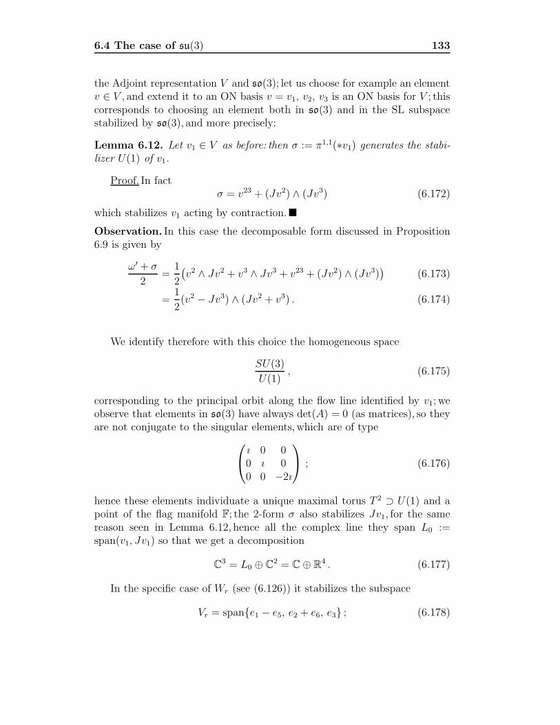
6.4 The case of su(3) 133
the Adjoint representation V and so(3); let us choose for example an elementv ∈ V , and extend it to an ON basis v = v1, v2, v3 is an ON basis for V ; thiscorresponds to choosing an element both in so(3) and in the SL subspacestabilized by so(3), and more precisely:
Lemma 6.12. Let v1 ∈ V as before: then σ := π1,1(∗v1) generates the stabi-lizer U(1) of v1.
Proof. In factσ = v23 + (Jv2) ∧ (Jv3) (6.172)
which stabilizes v1 acting by contraction.Observation. In this case the decomposable form discussed in Proposition6.9 is given by
ω′ + σ
2=
1
2
(v2 ∧ Jv2 + v3 ∧ Jv3 + v23 + (Jv2) ∧ (Jv3)
)(6.173)
=1
2(v2 − Jv3) ∧ (Jv2 + v3) . (6.174)
We identify therefore with this choice the homogeneous space
SU(3)
U(1), (6.175)
corresponding to the principal orbit along the flow line identified by v1; weobserve that elements in so(3) have always det(A) = 0 (as matrices), so theyare not conjugate to the singular elements, which are of type⎛⎝ı 0 0
0 ı 00 0 −2ı
⎞⎠ ; (6.176)
hence these elements individuate a unique maximal torus T 2 ⊃ U(1) and apoint of the flag manifold F; the 2-form σ also stabilizes Jv1, for the samereason seen in Lemma 6.12, hence all the complex line they span L0 :=span(v1, Jv1) so that we get a decomposition
C3 = L0 ⊕ C2 = C ⊕ R4 . (6.177)
In the specific case of Wr (see (6.126)) it stabilizes the subspace
Vr = spane1 − e5, e2 + e6, e3 ; (6.178)

6.4 The case of su(3) 134
moreover we can interpret the basis w1, w2, w3 as skew-symmetric endomor-phisms of C3 = R6 represented by the 2-forms:
w1 = −e13 + e53 − e24 + e64 (6.179)
w2 = −e14 + e23 − e36 + e45 (6.180)
w3 = e12 − e56 (6.181)
using the approach discussed in Proposition 6.11 we have in fact:
Lemma 6.13. Let Vr and Wr as before; then
π1,10 (Vr) = Wr . (6.182)
Proof.We have∧2V ∗
r = spane12 + e16 − e52 − e56, e23 + e63, e31 − e35 ; (6.183)
we do the projection:
π1,1(e12 + e16 − e52 − e56) = e12 − e56 = w3 (6.184)
π1,1(e23 + e63) = −e14 + e23 − e36 + e45 = w2 (6.185)
π1,1(e31 − e35) = −e13 + e53 − e24 + e64 = w1 (6.186)
hence the result.
We can finally prove Theorem 6.10:
Proof.The assertion regarding the local SU(3)-invariant isomorphism be-tween G2/SO(4) and SU(3) follows by just observing that both
G2
SO(4)\CP2 and SU(3)\S5 (6.187)
are tubular neighbourhoods of the singular orbit SSU (3 ) obtained by expo-nentiation of the same homogeneous vector bundle given by the standard3-dimensional representation of SO(3). For the second assertion we haveto prove that diagram (6.160) is commutative if we choose p1 in diagram(6.157); consider w3 ∈ Vr: this corresponds to
v1 = e3 (6.188)
v2 = e1 − e5 (6.189)
v3 = e2 + e6 (6.190)

6.4 The case of su(3) 135
referring to (6.178), therefore
e3 ∧ Je3 = e34 , (6.191)
hence L0 = spane3, e4;moreover((e1 − e5) − J(e2 + e6)
) ∧ J((e1 − e5) − J(e2 + e6)) (6.192)(
e1 − e5 + e1 + e5)) ∧ (e2 − e6) + e2 + e6)
) (6.193)
= 4e12 (6.194)
so that L1 = spane1, e2 and finally
L2 = spane5, e6 ; (6.195)
comparing this last with (6.126) and recalling that both the projections π2
and p1 πF are SU(3) equivariant, if they coincide at a point then they haveto coincide globally, hence the assertion follows.Observation.Let us denote by τ the element orthogonal to σ in t :
τ := −2e34 + e12 + e56 . (6.196)
In this case, (6.158) becomes
su(3) = t ⊕A1 ⊕ A2 ⊕ A2⊕ (6.197)
= spanσ, τ + [[L0L2]] + [[L0L1]] + [[L1L2]] (6.198)
= spanσ, τ + spane35 − e64, e36 + e45 (6.199)
+ spane13 − e42, e14 − e23 (6.200)
+ spane15 + e62, e16 + e25 . (6.201)
The Coincidence Theorem allows to identify the quaternionic span ofgrad f on the unstable manifolds; we want in this case to identify the elementof the Lie algebra which generate the Kvf spanning the imaginary part Im H ·grad f of this span in this specific example, in terms of the decompositionpreviously discussed:we observe that the matrix (6.125) belongs to t, whilethe two elements w1, w2 span a 2-dimensional space B1 lying in A1 ⊕A2; thefirst two components of Γ(x, y) instead span a subspace C1(x, y) which alongthe geodesic varies from B1 to A2.
Lemma 6.14. The quaternionic span Im H · grad f at the point Γ(x, y) isgiven by the Killing fields generated by
spanτ ⊕ C1 . (6.202)

6.5 Still open questions 136
Proof.The proof follows from the definitions just given and by observingthat σ is the stabilizer of the generic orbits along Γ, the Killing field generatedby (6.125) equals that of the orthogonal projection on τ .An immediate consequence is
Corollary 6.3. In the previous notation, we have
A0 ⊂ (H · grad f)⊥ (6.203)
at any point of M ⊂ G3(su(3)), where A0 denotes the Killing vector filedsgenerated by A0.
The quaternionic 4-form
Recall what discussed in Section 4.4: there a quaternionic 4-form is describedin purely algebraic terms (Proposition 4.4); recall that the critical submani-fold SSU (3 ) ⊂ G3(su(3)) corresponds to the subalgebras so(3) which give adecomposition
su(3) = so(3) ⊕ [Σ4] (6.204)
so that the tangent space TV G3(su(3)) for V = so(3) can be described as
TV G3(su(3))C = Σ2 ⊗ Σ4 ; (6.205)
comparing this with 4.83 we can conclude that Ω corresponds to the quater-nionic 4-form on G2/SO(4) to the tangent space restricted to SSU (3 ).
6.5 Still open questions
There are questions which have been left open, in the hope of finding morecomplete answers in the future.
i) First of all undersanding more precisely diagram 6.115,which expressesthe interplay between µ∗,µ∗, the the metric induced by the ambient Grass-mannian G3(g) and the QK metric.
ii) It would be also significant in this sense understanding more in deepthe role played by the conformal factor λ and the proportionality factora, which are clearly related in many cases (see Lemma 6.6).

6.5 Still open questions 137
iii) Another question is determining completely the quaternionic 4-formΩ described in 4.4 in this Grassmannian description, as the part we have de-scribed corresponds to the restriction to the submanifold SSU (3 ) (in factdΩ = 0).More in general: G3(g) has always b4 = 1 for g simple; what is therelationship between the invariant 4-form generating the cohomology and thequaternionic 4-form on the unstable submanifolds?
iv) Finally it would be interesting classifying completely the “generalizedsubalgebras” V satisfying grad gV = 0.

Bibliography
[1] M.F. Atiyah, N.J. Hitchin, I.M. Singer: Self-duality in 4-dimensional Rie-mannian geometry, Proc. R. Soc. Lond., A. 362 (1978), 425-461
[2] D.V. Alekseevsky:Compact quaternion spaces, Functional Anal. Appl.,2(1968), 106-114
[3] D.V. Alekseevsky:Quaternion Riemannian spaces with transitive reduc-tive or solvable group of motions, Functional Anal. Appl., 4(1970), 321-322
[4] D.V. Alekseevsky:Classification of quaternionic spaces with a transitivesolvable group of motions, Math. USSR-Izv., 9(1975), 297-339.
[5] D.V. Alekseevsky:Riemannian manifolds of cohomogeneity one, Colloq.Malh. Soc. J. Bolyai 56 (1989),9-22.
[6] A.V. Alekseevsky,D.V Alekseevsky:Riemannian G-Manifold with One-Dimensional Orbit Space, Ann. Global Anal. Geom., 11 (1993), 197-211
[7] D.V. Alekseevsky, S. Marchiafava, M.Pontecorvo: Compatible almostcomplex structures on Quaternion Kahler manifolds, Ann. Global. Anal.Geom., textbf16 (1998), 419-444
[8] V.I. Arnold:Mathematical methods in classical mechanics, Springer-Verlag, Berlin 1978.
[9] F. Battaglia: Applicazioni momento in geometria differenziale, PhDThesis, Firenze, 1993.
[10] F. Battaglia: Circle actions and Morse theory on quaternion-Kaler man-ifolds, J. London Math. Soc. (2) 59(1999), 345-358.
[11] F. Battaglia: S1 quotiens of quaternion-Kaler manifolds, Proc. Amer.Math. Soc. (7) 124(1996).

BIBLIOGRAPHY 139
[12] J. Berndt, S. Console, C. Olmos:Submanifolds and holonomy, Chapman& Hall/CRC, 2003.
[13] A. Besse: Einstein Manifolds, Springer-Verlag, 1987.
[14] G. E. Bredon: Introduction to compact transformation groups, Number46 in Pure and Applied Mathematics, Academic Press, 1972.
[15] R. Brylinski, B. Kostant: Nilpotent orbits, normality and Hamiltoniangroup actions, Bull. Lond. Math. Soc., 26(1992), 269-275.
[16] T. Brocker, T. tomDieck: Representations of Compact Lie Groups,Springer, 1985.
[17] F.E. Burstall, J.H. Rawnsley:Twistor Theory for Riemannian Symmet-ric Spaces, Lecture Notes in Mathematics 1424, Springer-Verlag, 1990.
[18] B.Y. Chen,T.Nagano: Totally geodesic submanifolds of symmetricspaces I, Duke Math. J., 44(1977), 745-755.
[19] B.Y. Chen,T.Nagano: Totally geodesic submanifolds of symmetricspaces II, Duke Math. J., 45(1978), 405-425.
[20] L. Conlon: The topology of certain spaces of paths on a compact sym-metric space, Trans. Amer. Math. Soc., 112 (1964), 228-248.
[21] D.H. Collingwood,M.W.McGovern:Nilpotent orbits in semisimple Liealgebras, Van Nostrand Reinhold, New York, 1993
[22] A. Dancer,A.F.Swann:Quaternionic Kaler manifolds of cohomogeneityone, Int. J. Math. 10 (1999), no. 5, 541-570.
[23] A. Dancer,A.F.Swann:HyperKaler metrics of cohomogeneity one, J.Geom. Phys., 21 (1997), 218-230.
[24] S.K. Donaldson:Nahm’s equations and the classification of monopoles,Commun. Math. Phys. 96 (1984), 387-407.
[25] J.J. Duistermaat, J.A. Kolk: Lie Groups, Springer, 2000
[26] E.B. Dynkin: Semisimple subalgebras of the semisimple Lie algebras,Amer.Math. Soc. Transl. Ser. 2, 6 (1952), 111-244
[27] H.D Fegan:The Laplacian with a Character as a potential and theClebsch-Gordan numbers, Quart. J. Math. Oxford (2), 34 (1983), 37-48

BIBLIOGRAPHY 140
[28] W. Fulton, J.Harris: Representation Theory. A first course, Springer,1991
[29] K. Galicki, B.Lawson: Quaternionic reduction and quaternionic orb-ifolds, Mat. Ann., 282(1988), 1-21.
[30] K. Galicki: A generalization of the momentum mapping construction forquaternionic Kaler manifolds, Commun. Math. Phys., 108(1987), 117-138
[31] A. Gray:A note on manifolds whose holonomy group is a subgroup ofSp(n)Sp(1), Michigan Math. J., 16 (1965), 125-128.
[32] W. Greub, S. Halperine,R. Vanstone: Connections, Curvature and Co-homology, vol. II and III, Academic Press, 1976.
[33] V. Guillemin, S. Sternberg: Symplectic techniques in physics, CambridgeUniversity Press, Cambridge 1990.
[34] R. Harvey, H.B. Lawson:Calibrated Geometries, Acta Math, 148(1982), 47-157
[35] S. Helgason: Differential Geometry, Lie Groups and SymmetricSpaces, AMS Graduate Studies in Mathematics Vol.34, 2001
[36] E. Heintze, R. Palais, C.-L. Terng, G. Thorbergsson:Hyperpolar actionson symmetric spaces, Geometry, topology and physics for Raoul Bott,(S.-T. Yau, ed.), International Press, Cambridge, (1995)
[37] E. Heintze, R. Palais, C.-L. Terng, G. Thorbergsson:Hyperpolar actionsand k-flat homogeneous spaces, J. Reine Angew. Math.454 (1994), 163-197
[38] R. Hermann:Variational completeness for compact symmetric spaces,Proc. Amer. Math. Soc. 11 (1960), 544-546.
[39] H. Herrera, R. Herrera:Classification of positive quaternion-Kahler 12-manifolds, C. R. Acad. Sci. Paris, Ser. I 334 (2002), 43-46
[40] H. Herrera, R. Herrera: A-genus on non-spin manifolds with S1 actionsand the classification of positive quaternion-Kahler 12-manifolds, J. Diff.Geom., 61 (2002), 341-364

BIBLIOGRAPHY 141
[41] N.J. Hitchin:Metrics on moduli spaces, in the “Lefschetz CentennialConference Part I: Proceedings on Algebraic Geometry, Mexico City,1984”, (Ed. by D. Sundararaman), Contemporary Math. 58, AMS,Providence, R.I., 157-178.
[42] N.J. Hitchin, A. Karlhede, U. Lindstrom, M. Rocek: Hyperkahler met-rics and supersimmetry, Commun. Math. Phys. 108 (1987), 535-589.
[43] R.A. Horn, C.R. Johnson:Matrix Algebra, Cambridge Univ Press, 1985
[44] S. Ishihara: Quaternion Kaahlerian Manifolds, J. Diff. Geometry, 9(1974), 483-500.
[45] D. Joyce: The hypercomplex quotient and the quaternionic quotient,Math. Ann. 290 (1991), 323-340.
[46] D. Joyce: Compact hypercomplex and quaternionic manifolds, J. Diff.Geometry, 35 (1992), 743-761.
[47] G. Ketsetzis, S.M. Salamon:Complex structures on the Iwasawa mani-fold, Adv. Geom., 4 (2002), 165-179
[48] F.C. Kirwan: Cohomology of Quotiens in Symplectic and AlgebraicGeometry, Princeton University Press, 1984
[49] P.Z. Kobak:Twistors, nilpotent orbits and harmonic maps, in “Har-monic maps and integrable systems” (A. P. Fordy and J. C. Wood, eds.),Aspects of Mathemtics, vol. E 23, Vieweg, Braunschweig, Wiesbaden,1994, 295-319.
[50] P.Z. Kobak,A.F.Swann: Quaternionic geometry of a nilpotent variety,Math. Ann., 297(1993), 747-764.
[51] P.Z. Kobak, A. F. Swann, Classical nilpotent orbits as hyperKhler quo-tients, International J. Math. 7 (1996), 193-2l0
[52] P.Z. Kobak,A.F.Swann: Hyperkahler potentials in cohomogeneity two,J. Reine Angew. Math. 531 (2001), 121-139.
[53] P.Z. Kobak,A.F.Swann: Hyperkahler potentials via finite-dimensionalquotiens, Geom. Dedicata 88 (2001), 1-19.
[54] P.Z. Kobak,A.F.Swann: The HyperKahler Geometry Associated toWolf Spaces, Bollettino U. M. I. (8) 4-B (2001), 587-595.

BIBLIOGRAPHY 142
[55] S. Kobayashi,K. Nomizu: Foundations of Differential Geometry, vol. Iand II, Interscience Publishers, 1963, 1969.
[56] A.A. Kollross:A classification of hyperpolar and cohomogeneity one ac-tions, Trans. Am. Math. Soc., 354 (2001) 571-612.
[57] B. Kostant: The principal three-dimensional subgroup and the Bettinumbers of a complex simple Lie group, Amer. J. Math. 81 (1959),973-1032.
[58] P.B. Kronheimer: Instantons and the geometry of the nilpotent variety,J. Diff. Geometry, 32(1990), 473-490.
[59] C.R. LeBrun: Quaternionic-Kahler manifolds and conformal geometry,Mat. Ann., 284(1989), 353-376.
[60] C.R. LeBrun, S. Salamon: Strong rigidity of positive quaternion-Kahlermanifolds, Invent. Math. 118 (1994), 109-132.
[61] M. Mamone Capria, S.M. Salamon:Yang-Mills fields on quaternionicspaces, Nonlinearity, 1 (1988), 517-530.
[62] S. Marchiafava,G. Romani: Sui fibrati con struttura quaternioniale gen-eralizzata, Ann. Mat. Pura Appl. 107 (1976), 131-157.
[63] W.S. Massey:Non-existence of almost-complex structures on quater-nionic projective spaces, Pacific J. Math., 12 (1962), 1379-1384.
[64] Y. Nagatomo: Private communication.
[65] Y. Nagatomo: Instanton moduli on the quaternion Kahler manifold oftype G2 and singular set, Math. Z., 243 (2003), 243-261
[66] Y. Nagatomo:Vanishing theorem for cohomology groups of c2-self-dualbundles on quaternionic Kahler Manifolds, Differential Geom. Appl. 5(1995), 79-95
[67] Y. Nagatomo: Representation theory and ADHM-construction onquaternion symmetric spaces, Trans. Amer. Math. Soc. 353 (2001),4333-4355
[68] R.S. Palais, C.-L. Terng: A general theory of canonical forms , Trans.Amer. Math. Soc., 300 (1987), 771-789.
BIBLIOGRAPHY 143
[69] Y.S. Poon, S.M. Salamon: Eight-dimensional quaternionic-Kahler man-ifolds with positive scalar curvature, J. Diff.Geometry, 33(1991), 363-378.
[70] M. Pontecorvo:Complex structures on quaternionic manifolds, Diff.Geom. Appl., 4 (1994), 163-177
[71] S.M. Salamon: Quaternionic Kahler manifolds, Invent. Math., 67(1982),143-171.
[72] S.M. Salamon:Differential geometry of quaternionic manifolds, Ann. sci-ent. Ec. Norm. Sup. 19 (1986), 31-55.
[73] S.M. Salamon: Riemannian Geometry and Holonomy Groups, PitmanResearch Notes in Mathematics 201, Longman Scientific, 1989.
[74] S.M. Salamon:Almost parallel structures, in: Global differential geom-etry: the mathematical legacy of Alfred Gray (Bilbao 2000), Contemp.Math. 288, Amer. Math. Soc., Providence R.I. 2001, 162-181.
[75] S.M. Salamon:Quaternionic structures and twistor spaces, Global Rie-mannian Geometry, ed. T.J. Willmore and N. Hitchin (Chichester: EllisHorwood), 1984.
[76] I.M. Singer, J.A. Thorpe:The curvature of 4-dimensional Einsteinspaces, “Global Analysis. Papers in honor of K.Kodaira (Ed. D.C.Spencer, S. Iyanaga), Princeton University Press, 355-365
[77] A.F. Swann:Private communication.
[78] A.F. Swann: Aspects symplectiques de la geometrie quaternionique, C.R. Acad. Sci. Paris, 308(1989), 225-228.
[79] A.F. Swann: HyperKaler and quaternionic Kaler geometry, Math. Ann.,289(1991), 421-450.
[80] A.F. Swann: Homogeneous twistor spaces and nilpotent orbits, Math.Ann., 313(1999), 161-188.
[81] F.W. Warner:Foundations of Differentible Manifolds and Lie Groups,Springer-Verlag, 1983
[82] R.O. Wells:Differential Analysis on Complex Manifolds, Springer-Verlag, 1980

BIBLIOGRAPHY 144
[83] J.A. Wolf: Complex Homogeneous contact structures and quaternionicsymmetric spaces, J. Math. Mech. 14(1965), 1033-1047.