Decision making with incomplete information...46 M. Weber / Decision making with incomplete information will use the symbol Zi for the name of the attri- bute as well as for the evaluator

44 European Journal of Operational Rcscarch 28 (1987) 44-57 North-Holland

Decision making w ith incomplete information Martin WEBER Lehr- und Forschungsgebiet Allgemeine Betriebswirtschaftslehre, R WTH Aachen, Templergraben 64, 5100 Aachen, Germany, Fed. Rep.

Abstract: Decision situations with incomplete information are characterized by a decision maker without a precisely defined, stable preference structure; by probability distributions not known completely; or by an inexact evaluation ‘of consequences. Within the paper a general framework for decision making with incomplete, information is presented which shows how to solve problems from descriptive as well as prescriptive decision theory. Based on this framework an overview of existing methods which are particularly suitable for handling incomplete information is given.

Keywords: Decision, information, decision theory

1. Introduction

There are many methods in the field of decision analysis .that try to help a decision maker to come up with a decision, that is, to find an optimal or satisfying solution. However, if one compares the amount of theoretical ,work being done to develop new methods and theories with the degree of their practical acceptance one quickly realizes that a gap between theoretical research and practical needs exists. This gap’could be due to the fact that decision analysis is a relatively new field and recent developments have not yet been transferred to industry. Another possibility is that the decision problem or the preferences of the decision maker (DM) are not.(yet) structured enough to allow the successful application of most decision analysis methods; For’ example,, the DM can not provide exact estimations of probability distributions or he/she is not willing or able to specify the preferences in ‘the detailed way required by the corre- spanding~ method. To narrow the gap between theoretical research and industrial needs and ap- ‘plications we want to present and discuss a specific class of decision models that can be used within decision situations having partial, incomplete in-

Rekeived February 1985; revised November 1985

formation on parameters which describe the decision situation.

Traditionally in the world of complete, exact information a decision situation is characterized by a given set of alternatives, a set of objectives (attributes), a known probability distribution of the outcomes and a DM (or a group of DMs) having a stable preference structure. Within the framework of prescriptive decision theory, methods’ should help a DM to find an optimal or satisfying solution. Expected utility theory, and subjective expected utility theory (Fishburn, 1983; Raiffa, 1968; Schoemaker, 1982; von Neumann and Morgenstern, 1953) must be considered the leading paradigm for prescriptive decision theory. However, utility theory requires the DM to provide all information describing the decision situation. It is obvious that this information require- ment is much too strict in most practical applications, because the probabilities can not be esti- mated exactly, the DM has not yet made up his/her m ind, or the set of alternatives is not completely defined, etc. This means that traditional subjective expected utility theory can hardly be applied successfully. Using subjective expected utility theory could therefore result in adapting reality to the model.

Within the descriptive branch of decision theo- rem one tries to describe or predict human behavior that is empirically observable. Taking market-

0377-2217/87/$3.50 0 1987, Elsevier Science Publishers B.V. (North-Holland)

M. Weber / Decision making wirh incomplete informatiotl 45

ing research as an example for an area where results of descriptive decision theory are applied, the aim is to determine the set of consumers’ objectives and ultimately to predict his/her buying behavior. Methods currently used to estimate consumer preferences such as conjoint analysis (see Green and Srinivasan, 1978) try to infer the preferences from consumers’ holistic (ordinal or cardinal) statements. However, these procedures based on traditional utility models do have two main deficiencies: Firstly they force the consumer to provide exact evaluations regardless of whether he/she has already made up his/her mind or not. So the ‘exact’ prediction can be an artifact of the model. Secondly, as these models treat people with stable and unstable preference structures alike they do not allow for .inferring the consumers uncertainty over the relevance of product attributes from their stated preferences. Obviously, it would be useful in develbping market strategies to know which parts of the consumer preferences are relatively stable and ,which are not. Modern decision theory has recognized these deficiencies bf traditional subjective expected utility theory (SEU theory) and researchers have proposed different strategies to overcome the problems. Within this paper we will focus on one main stream of devel- opment that is still based on subjective expective utility theory. We will discuss models which do not require the DM to provide exact statements about probability distributions and/or preference judgements. So the idea of this line of research is basically that we should stick to the advantages of SEU theory, which is thoroughly axiomized widely tested and known. At the same time we will try to weaken the strong information requirements and thereby make the theory more applicable to practical problems. If the information is available only in an inexact, incomplete or partial manner we will talk about decision making with incomplete information. Exact definitions will be given in the second section.

There are other mainstreams of decision theory research not directly based on SEU where work is being done on more applicable theories to explain a DM’s behavior and/or help a DM to decide. As it is not our purpose here to discuss all recent developments we just want to mention a few names. For an overview on fuzzy set theory see e.g. Zadeh (1965) and Zimmermann (1983). An overview and comparison of traditional probabilities with fuzzy

probabilities, possibilities and other forms of uncertainty treatment in decision theory is given by Freeling (1984) and Gaines (1984). A first attempt to integrate different streams like fuzzy set theory, theory of evidence (Shafer, 1976) and decision with incomplete information on probabilities can be found in Einhorn and Hogarth (1985).

Coming back to decisions with incomplete information, recent work has focused on three major problems: First, the need for a general model (framework) for decisions with incomplete information; second the need for methods to help a DM find an (optimal) solution (prescriptive aspect); and third, the need for methods designed for newly defined descriptive problems. Taking these three aspects the rest of the paper will be organized as follows. In Section 2 a general model for decision making with incomplete information is presented. Prescriptive and descriptive aspects of decisions with incomplete probability distributions are discussed in Section 3 while Section 4 explores decision making for incomplete preference structures. Section 5 contains suggestions for future research.

2.‘ A general model for decision making wivith incomplete information

Within this section we first want to recapitulate SEU theory and then extend it to decisions with incomplete information. Finally three main steps for solving decision problems with incomplete information are presented.

Let A be the given set of alternatives A = {a, b, c, . . . } which the DM has to decide upon and s= {s,,..., s,,, } be the given set of all possible states of the world. The probability pj that state sj E S occurs is given by the function p : S --, [OJ].

For reasons of simplicity we will assume both sets to be finite. The consequence of alternative a E A if state s E S occurs is given by ,a function g. Since in most situations there is more than one attiibute (which we will equate with ‘objective’ and ‘goal’), the consequence g(a, s) has to be represented by an attribute vector. Taking Z = {Z,,..., Z,, } as the set of attributes, g is a function from A X S + Z, X . * . X Z,,, i.e. g(a, sj) = aj=(a,j,..., a,,]) where aj denotes the consequence of a for state sj. In the case of certainty,

‘S-={s}andwewilljustwritea=(a,,...,a,,):We

46 M. Weber / Decision making with incomplete information

will use the symbol Zi for the name of the attribute as well as for the evaluator of the same attribute.

Given the data in the above way the DM has to aggregate them according to his/her preferences. Therefore our goal is to determine an aggregation function f, which reflects the preferences of the DM in aggregating the data and allows the ranking of alternatives, i.e. a t b ef( a) >f(b); a, b E A. From a prescriptive point of view f proposes an optimal alternative and from a descriptive viewpoint f describes the DM’s behavior.

To determine the function f four questions have to be answered either implicitly or explicitly:

(i) What is the value of the consequence aj on attribute Zi. (For example, taking money as an attribute, what is the value of getting 10 Deutsch Marks compared to 20 Deutsch Marks?)

(ii) What is the decision maker’s risk attitude? How does the DM evaluate the risk attached to the decision situation?

(iii) What is the aggregation of evaluation on different attributes for each consequence?

(iv) What is the aggregation of the consequences of each alternative?

Within SEU theory f is defined as expected utility:

j-l

where u is the DM’s utility function; u: Z, X . . . XZ,+W and we have u>b-E(u)(u))> E(u(b)); a, b E A. Utility theory simultaneously measures aspects of value and risk, so that the answer to questions (i) and (ii) are intertwined. The answer to (iv) follows immediately from the axioms of SEU; it has to be an additive form. The aggregation over attributes (question (iii)) depends on the structure of the set of attributes. For reasons of simplicity we will - without loss of gener- ality - assume that the attributes are additive independent (Keeney and Raiffa, 1976) which leads to an additive multiattribute utility function:

n “(Uj) = c kiU,(Uij).

i-l

If there is only one state of the world, meaning we consider decisions under certainty, then we need a slightly different axiomatic system to define f. To distinguish certainty from uncertainty some

authors talk about value functions and we get a similar additive representation for a mutual independent set of attributes (see, Dyer and Sarin, 1979; Keeney and Raiffa, 1976, for further details). As long as there is no need to distinguish between different axiomatic systems we will just talk about utility functions and utility theory.

Recapitulating the framework for SEU theory, a decision-situation is completely defined by the sets A, S, Z and the functions u, p and g. As mentioned earlier, we will call a decision situation incomplete if and only.if at least one of the functions u, p or g is not exactly specified. For example the DM may not be sure about the utility function either because he/she allows a range for the weights of the conditional utility functions ui; or he/she is not sure about risk and value judgements on one or several attributes. Or regarding the probability distributions, there may only be ordinal information or interval statements on the probability of the states available. Finally, looking at g, the DM may not be sure about how the consequence of an alternative should be evaluated in the attribute space. Throughout this paper we will assume however that the sets A, S and Z are given. To consider incomplete sets A, S and Z as well, is a possible extension of the model presented in this paper.

Given certain information I available in a specific decision situation the classes (sets) of functions u, p and g which are consistent with the information are denoted by U(I), P(I) and G(Z). Within the general model we will consider the possibility of an incomplete evaluation function g. Such a function would be called incomplete if there is more than one consequence for at least one pair (a, s’) E A X S. As this case is, to our knowledge, not (yet) discussed in the literature we will not dedicate a special section to it. The literature has dealt with only some aspects of the incomplete decision situation described here. Though no definite terminology has been developed for the general case, some authors talk about ‘partial information’ (Hazen, 1983b; Kirkwood and Sarin 1985), ‘imprecise information’ or ‘incomplete knowledge’ (Kmietowicz and Pearman, 1981) meaning incomplete information on utility or probability functions in our terminology.

Based on SEU theory we will now define several dominance relations which allow the deduction of preference statements on pairs of alternatives. If

M. Weber / Decision making with incomplete information 47

for each utility function out of the set of all utility functions consistent with the available information the expected utility of an alternative a is greater than the one of a second alternative 6, that is, a is preferred to b for all u E U(I), we could say ‘a is preferred to b with respect to U(I)’ or ‘u + uc,,b’. Similar considerations for P(I) and G(1) lead to an extension of the Bernoulli principle (maximize expected utility) for decisions with incomplete information:

a>b e Eb(4) ’ E(u(b)), foralluEU(I);pEP(I)andgEG(I).

If for each combination of g, p and u which is consistent with the information, a is preferred to b, then we will say alternative a dominates b with respect to U(1), P(I) and G(I). If there is a need to distinguish this dominance concept from others we will call this dominance Bernoulli dominance.

A second form of dominance can be defined, if we calculate the two alternatives’ expected utility independently. We will call this dominance ‘absolute dominance’:

a>b - +(a)) > E( u’(b)), forall 2.4, z/E U(I); p, p’EP(I)

and g, g’c G(I),

or 2 pju(g(a, sj))> 5 Pju’(g’(Q, sj>),

j=l j=l

Alternative a is absolutely preferred to b (a dominates b absolutely), if the minimal expected utility of a is greater than the maximal expected utility of 6. It is easy to show that dominance and absolute dominance are irreflexive, asymmetrical and transitive relations. Clearly the set of absolutely dominated alternatives is a subset of the set of dominated alternatives.

If we now equate the set of non-dominated alternatives to the set of potential optimal alternatives, we could be wrong. For some alternatives it could follow that they are not dominated, however, for every feasible combination of U, p and g there exists at least one alternative which is preferred (see Fishburn (1964) for mixed strategies). Calling this mixed dominance we can define:

A’>,b - forall UE U(I), PEP(I) and gE G(I) thereis a EA’ with E(u(a))>E(u(b)); A’CA.

If for each feasible combination of U, p and g there is one alternative a element of a subset A’ of A, having greater expected utility than b, then we will say that A’ dominates b. Clearly mixed dominance follows from dominance. As seen later stronger dominance conditions generally could be checked more easily and therefore they might sim- plify the determination of the existence of weaker dominance relations.

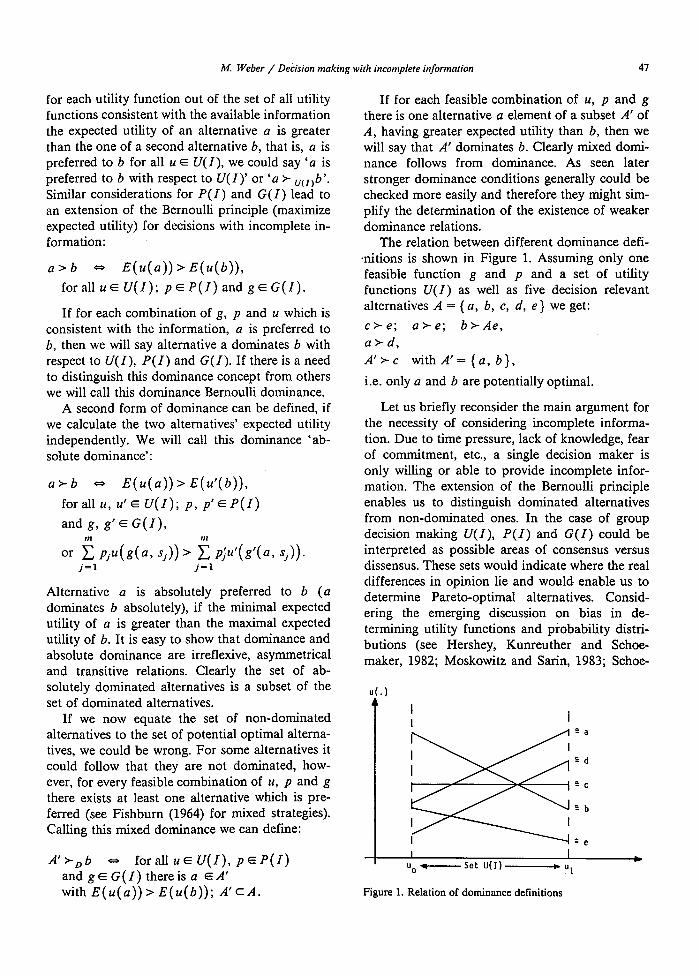
The relation between different dominance definitions is shown in Figure 1. Assuming only one feasible function g and p and a set of utility functions U(I) as well as five decision relevant alternatives A = {a, b, c, d, e} we get: c>e; a>e; b>Ae, at d, A’>c with A’= {a, b}, i.e. only a and b are potentially optimal.

Let us briefly reconsider the main argument for the necessity of considering incomplete information. Due to time pressure, lack of knowledge, fear of commitment, etc., a single decision maker is only willing or able to provide incomplete information. The extension of the Bernoulli principle enables us to distinguish dominated alternatives from non-dominated ones. In the case of group decision making U(I), P(I) and G(I) could be interpreted as possible areas of consensus versus dissensus. These sets would indicate where the real differences in opinion lie and would enable us to determine Pareto-optimal alternatives. Consid- ering the emerging discussion on bias in de- termining utility functions and probability distributions (see Hershey, Kunreuther and Schoe- maker, 1982; Moskowitz and Sarin, 1983; Schoe-

ut.1

t I I

Figure 1. Relation of dominance definitions

48 M. Weber / Decision making wifA incomplete bl/ormatiotl

maker, 1980) a set U(I) or P(I) could be interpreted as the possible range of bias observed by a DM.

From the descriptive point of view U(I) could be the set of all utility functions representing the (yet) unstable preference judgements of a DM. Despite these incomplete preferences we could use dominance rules to exactly predict a range of possible behavior by excluding some alternatives from being chosen. There is preliminary empirical support that DMs want to use the concept of incomplete information for assessing their utility functions. In a multi-attribute decision making situation 21 out of 22 German students provided incomplete information while being put in a prescriptive and a descriptive decision situation (Weber, 1983b). In a study to predict the buying behavior of American MBA students 23 out of 33 voluntarily chose to provide incomplete information through interval judgments (Currim and Weber, 1985).

Returning to the goal of extending expected utility three main questions have to be discussed and answered before we can apply the concept:

(i) In which way are we able to measure or define the sets of utility, probability and evaluation functions?

Taking the set of probability functions first, we could either elicit a (partial) ranking of probabilities (i.e. pi is greater than pi) or get interval statements on probabilities (i.e. pi lies in the interval IP;, p’], see (Sarin, 1978)). Beside these ‘pure’ forms we could receive a combination or ordinal and interval information or, more generally, the information could be represented by a complex system of equations (i.e. f( pi,. . . , pj) = or > constant). Considering the case of incomplete information about preferences the set U( 1) can be defined implicitly by a general property of utility functions, such as the risk attitude of the DM. For second degree stochastic dominance, the set U(I) is defined as the set of all risk averse, monotoni- cally non-decreasing utility functions (Fishburn and Vickson, 1978). Obviously specific ways of defining the sets require specific measurement theories to elicit the information. However, in applying different theories for incomplete utility and probability measurement, one would have to be aware of possible interaction effects. If theories are already developed, we will mention them in the next two sections.

If we have determined the set of functions the next question to be solved is:

(ii) How can we check different types of dominance depending on the way we defined the sets of utility, probability and evaluation functions and the way we elicited the information?

The answer to this question is the central point of interest of research on decision with incomplete information. If we would succeed in providing simple rules for checking dominance the concept could be easily applied to reduce the decision relevant set of alternatives. We therefore will stress this point in the next two sections.

Depending on the size of the sets of utility, probability and evaluation functions the induced relation on A x A will be more or less complete. If the DM is not willing to provide more information in an additional round it could happen that the choice or an exact prediction can only be made using decision rules.

So, as a third question, we state: (iii) How can we derive a complete relation

(ranking of alternatives) based on the information we received up to this point?

We can distinguish two classes of decision rules. Rules of type number one begin with calculating maximal and minimal expected utilities (with respect to U(I), P(I) and G(I)) for each non- dominated alternative. Applying decision-rules for decision making under uncertainty (see e.g. (Lute and Raiffa, 1957, pp. 297) we can get the optimal alternative or the ranking of the alternatives.

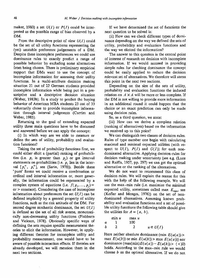
We do not want to recommend this class of decision rules. We will explain the reason for this with the help of the following example. We will use the max-min rule (i.e. maximize the minimal expected utility, sometimes called max E,,, see (Kofler and Menges, 1976)) on the set of non- dominated alternatives. Assuming known probability and evaluation functions and a set of possible utility functions the following table should give the utilities for A = {a, b}.

minu maxu 1

5 2 100

2 UE U(I)

.Here neither absolute dominance (min E( U( a)) > max E(u(b)) or min E(u(b))> max E(u(a))) nor dominance (max(min)E(u(a))-E(u(b))> (c)o) holds. According to the max-min rule we would choose b as the optimal alternative. If we. do not


want to consider only the minimal utilities, a is preferred to b for most utility functions consistent with the available information. So we should feel better in incorporating all information received up to this point and based on this information, to develop a measure for the strength of preference between alternatives. A final ranking should be derived in a way which best fits this measure. Our second class of decision rules will contain those rules that are based on a measure of strength of preference and do not only consider one extreme value for each alternative.

To come up with a measure of strength of preference between pairs of alternatives let h be a function that gives the difference of expected utilities between two alternatives a and b for given functions u, p and g:

h(a, b, u, P, s> = E(u(a)) -E(u(b)),

forall a, bEA; UE U(I);

p E P(I) and gE G(I).

The measure of the strength of preference for a over b is defined as a function d: A x A + [0, 11:

d(a, b)= P(h(a, b, a, a, a)> 0), where P(e) is the probability, that h(a) is greater than or equal to 0.

d depends on the distribution over the interval bin E(u(a)) -E(u(b)), mm ECU(a))-- ECu( and therefore takes into account all information provided by the DM up to this point. Without considering G(1) it has to be assumed that some distributions over U(I) and P(I) exist. To derive the distribution of h we suggest that the density functions on V( 1) and P(I) are assumed to be constant. d(a, b) is equal to 1, if and only if the alternative b is dominated by a.

The problem of deriving a ranking of the alternatives via the values given by the function d, is equivalent to the broadly discussed problem of aggregating individual group member’s rankings on alternatives to a (transitive) group ranking. Therefore different procedures to calculate a ranking of the alternatives have already been developed (Bowman and Colantoni, 1973; Goddard, 1983; Marcotorchino and Michaud, 1979). Most procedures differ mainly in their definition of similarity. To give a concrete example, we will discuss perhaps the easiest procedure which de- fines similarity by the /,-norm (see (Liebling and Rossler, 1978) for the exact algorithm).

For any pair of alternatives a, b E A if d(a, 6) > 0.5 we assume a dominates b, and if d(a, b) < 0.5 we assume b dominates a. If d(a, b) = 0.5 we can arbitrarily assume a dominates b. If the resulting relation is intransitive we have to find the cycle in the graph representing the relation (a > b > c > a). We now have to change the dominance relation of this pair which has the lowest underlying d value. We have to go on changing the dominance relations until the remain- ing relation is transitive, and we can thus derive a ranking.

Within the next two sections we will specify the general procedure presented in this section and apply it to decision making with incomplete information on probability functions or utility functions.

3. Decision making with incomplete information on probability distributions

Decision making with incomplete information on probability distributions lies somewhat between decision making under uncertainty (P(1) + set of all possible probability distributions, no information) and decision making under risk (1 P(I) I= 1, complete information). Within this section we want to briefly present methods for decision making based on sets of probability distributions. Refer- ences for more detailed descriptions are given throughout this section. In addition we have to focus on the prescriptive point of view. Even for complete information there are hardly any papers which try to predict behavior using expected utility theory (see (Currim and Sarin, 1984; Hauser and Urban, 1979) as exceptions).

Coming to the first question ‘how to measure incompl’ete information?‘, it should be no problem to elicit ordinal and/or interval judgements on probabilities. A problem exists if we want to know whether there are any probability distributions consistent with this information, that is, whether these judgements elicited are compatible with the laws of probability theory. For ordinal information on the probabilities of the states s, there always exists a non-empty set of distributions (Biihler, 1976). For necessary and sufficient conditions for the existence of probability distributions based on ordinal information on subsets of S (Wollenhaupf 1982), interval evaluations of sj

50 M. Weber / Decision making with itrcotttplete inforttmtion

(Good, 1962) and ordinal and interval judgements on sj (Wollenhaupt, 1982) the reader is referred to the literature.

If the set of feasible probability distributions is non-empty and contains more than one element (the information is incomplete) dominance relations have to be checked. Based on Fishburn (1964) different authors suggest verifying dominance with the help of linear programming (Jacob and Kar- renberg, 1977; Kmietowicz and Pearman, 1981; Potter and Anderson, 1980). For example with ordinal and interval information on the probabilities of the states sj, dominance might be checked with the following LP model:

tn mm (n+ C pj("(uj)-u(bj)),

j-l

tn Cpj=l, j,i=l,..., tn; j+i.

j-l

To check all dominance relations as a maximum one has to solve 1 A /(I A 1 - 1) small linear pro- grams. The number in general reduces if one is only interested in an optimal alternative or checks absolute dominance first. Absolute dominance can be verified easier (21 A I LPs to be solved) using the following two objective functions:

tn ma (tin> C Pj"(aj),

j-l

s.t. same restrictions. Sometimes it might be appropriate or necessary

to check dominance without using an LP model. One approach is described by Kofler and Menges (1976); see also Kmietowicz and Pearman (1984), who define incomplete information - they call it linear partial information LPI - by a system of restrictions:

tn C~.ljPj>k,, I=l,...,r; r>m,

j-1

tn CPj=l,

j-l

where x,~ and k, are parameters elicited from the DM. A dominance check with respect to the (whole) LPI is equivalent to a check with respect to some specific probability distributions arising at corner points of the feasible region defined by the LPI. Kofler and Menges give an algorithm to determine the corner points with which dominance might be checked (see (Btihler, 1975; and Sarin, 1978) for similar results).

Sarin (1978) examines decision situations where the incomplete information is either given by a ranking of the probabilities of the states or by an interval evaluation of the same probabilities. For these cases he gives two criteria to check dorni- nance which can be easily applied. Taking the case of ordinal information described above and assuming the probabilities are arranged in a de- scending order (i.e. pi 2 pi+,), we can state:

j-1 - j-1

forall t=l,...,m.

Sarin (1978) develops similar simple conditions for the situation in which the probabilities depend on the alternatives.

In case the induced dominance relation is not sufficient to solve our decision problem we have to determine an optimal alternative or a (complete) ranking with the help of some additional decision rules. Whereas some authors (Sarin, 1978) do not pay much attention) to this point others emphasize this question. Especially in the German literature there is a discussion whether to use the max E,i”- rule (Btihler 1976, 1981; Firchau, 1985; Kofler and Menges, 1976), the Laplace rule (Sinn, 1980) or some mixed rules (Jacob and Karrenberg, 1977). All these rules, however, apply rules for decision making under uncertainty to this ‘uncertain’ part of decision making with incomplete information, to those problems where the information received is not (yet) complete enough. Not much is done to incorporate ail information received up to this point, in other words, to use the concept of strength of preferences between pairs of alternatives (described in Section 2) to determine a ranking. Kmietowicz and Pearman’s (1984) concept of ‘weak dominance’ could be seen as belonging to this class. They say a is weakly dominating b if and only if maxlE(u(a))-E(u(b))l is greater than maxlE(u(b))-E(u(a))l or in our termi-

M. Weber / Decision making with itrcomplete information 51

nology if and only if maxi h (a, b, p) 1 is greater than max Ih(b, a, p)I for all PEP(I). If one now assumes the distribution over the interval [tin ECU(~)) - E(u(b)), mm ECU(U)) - E(u(b))] to be rectangular the relation derived from the d-function is equal to the one induced by weak dominance.

4. Decision making with incomplete information on utility functions

Within this section we want to focus on decision making with incomplete information on utility functions. First it has to be discussed why the DM does not always provide complete information. What do we measure if we observe incomplete information on preferences? Next we will present methods to help a DM to come up with a decision (prescriptive aspect). Methods that predict on the basis of incomplete information are described in the last part of this chapter.

4.1. Incomplete information on utility functions - What does it mean?

From the prescriptive point of view this question is not particularly interesting. A method is used here to help a DM to find his/her optimal alternative. In case he/she can already propose one unique optimal alternative, perhaps with some interactive procedure, there is no need to ask for more information. We would just hypothesize that the DM prefers providing less information to more information and he/she would therefore prefer methods based on incomplete information. If we are only able to reduce the set of decision relevant alternatives to a subset and the DM has asked us to leave his/her office for he/she is bothered by our penetrating questions, then it is primarily un- important for this decision situation why no more information is provided. To adapt the information gathering process, however, to the DM it is definitely important to know what causes the incompleteness of the information. Is it a result of the DM’s headache, or the DM’s fear to decide exactly, or the DM’s not yet fully developed preferences? This leads to the more descriptive question: What does the observed incompleteness mean? An answer is especially important if we want to pre- scribe some (future) behavior based on the incomplete information.

In measuring incomplete information on preferences we could measure a real psychological con- struct but we could also measure some artifact of our ‘strange’ way of interrogating the DM. There- fore we first have to discuss the relation between observed incompleteness and an underlying ‘true’ incomplete preference structure, and then some theoretical considerations will be presented.

Getting a set of utility functions can be due to the fact that the DM has a complete, exact structure but he/she does not want to properly com- municate with the decision analyst. This can be the result of factors like: time pressure, the reluctance to use formal methods, the headache mentioned above or the unwillingness to have one’s own opinion too open to criticism etc.

In case a DM is delighted by the method and he/she has an exact preference structure, the incompleteness can result from problems attached with the interrogation procedure. For example the DM is asked to evaluate hypothetical, irrelevant alternatives like ‘what do you think about a Mercedes which costs 10000 Deutsch Marks and consumes no gas? or the presentation of an (artifi- cial) alternative is done so poorly that the DM can not relate it to a real decision situation.

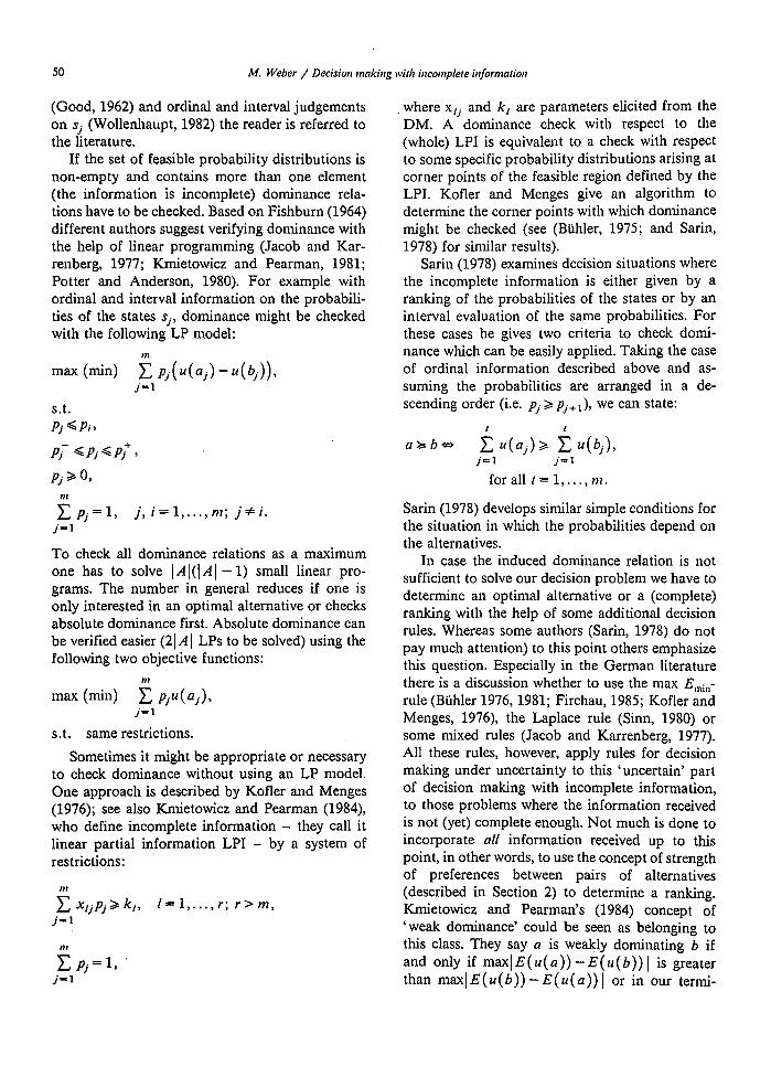
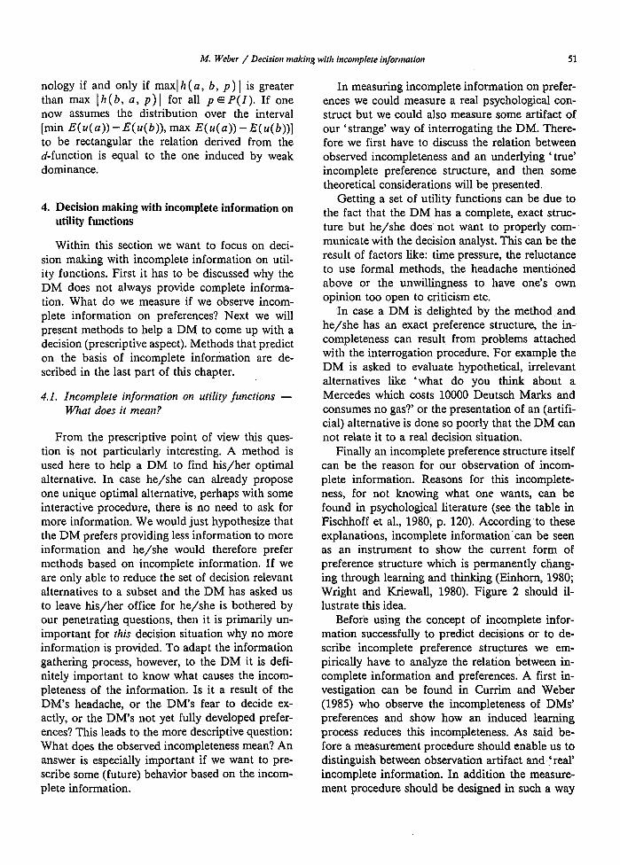
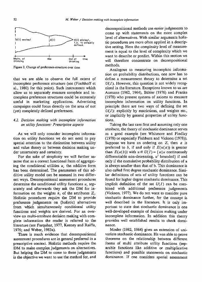
Finally an incomplete preference structure itself can be the reason for our observation of incomplete information. Reasons for this incompleteness, for not knowing what one wants, can be found in psychological literature (see the table in Fischhoff et al., 1980; p. 120). According to these explanations, incomplete information’can be seen as an instrument to show the current form of preference structure which is permanently cliang- ing through learning and thinking (Einhom, 1980; Wright and Kriewall, 1980). Figure 2 should il- lustrate this idea.

Before using the concept of incomplete information successfully to predict decisions or to describe incomplete preference structures we empirically have to analyze the relation between incomplete information and preferences. A first investigation can be found in Currim and Weber (1985) who observe the incompleteness of DMs’ preferences and show how an induced learning process reduces this incompleteness. As said before a measurement procedure should enable us to distinguish between observation artifact and ‘real incomplete information. In addition the measurement procedure should be designed in such a way

52 M. Weber / Decisiorl snaking wit/r inconlplere infomarion

I

Begin.. Of thinking

I I NOW

I I .

End of t ime thinking

Figure 2. Change of preference-structure over time

that we are able to observe the full extent of incomplete preference structure (see (Fischhoff et al., 1980) for this point). Such instruments which allow us to separately measure complete and incomplete preference structures could be extremely useful in marketing applications. Advertising campaigns could focus directly on the area of not (yet) completely defined preferences.

4.2. Decision making with incomplete information on utility functions: Prexriptive aspects

As we will only consider incomplete information on utility functions we do not need to pay special attention to the distinction between utility and value theory or between decision making under uncertainty and certainty.

For the sake of simplicity we will further assume that as a correct functional form of aggregating the conditional utilities ui the additive form has been determined. The parameters of this additive utility model can be assessed in two different ways. Decompositional assessment procedures determine the conditional utility functions ui separately and afterwards they ask the DM for information on the weights ki of the attributes Zi. Holistic procedures require the DM to provide preference judgements on (holistic) alternatives from which simultaneously conditional utility functions and ,weights are derived. For an overview on multi-attribute decision making with complete information the reader is referred to the literature (see Farquhar, 1977, Keeney and Raiffa, 1976; and Weber, 1983a).

There is much evidence that decompositional assessment procedures are in general preferred in a prescriptive context. Holistic methods require the DM to make complex judgements on alternatives. But helping the DM to come to these judgements is the objective we want to use the method for, and

decompositional methods use easier judgements to come up with statements on the more complex level of alternatives. With similar arguments holistic procedures are more often applied in a descriptive setting. Here the complexity level of measurement is equal to the level of complexity which we want to describe or predict. Within this section we will therefore concentrate on decompositional methods.

Analogous to measuring incomplete information on probability distributions, one now has to define a measurement theory to determine a set U(1). However, this question is not widely recognized in the literature. Exceptions known to us are Aumann (1962, 1964), Biihler (1976) and Franke (1978) who present systems of axioms to measure incomplete information on utility functions. In principle there are two ways of defining the set U(I): explicitly by restrictions, and weights etc., or implicitly by general properties of utility functions.

Taking the last case first and assuming only one attribute, the theory of stochastic dominance serves as a good example (see Whitmore and Findlay (1978) or especially Fishburn and Vickson (1978)). Suppose we have an ordering on Z, then a is preferred to 6, if and only if E( u(a)) is greater than E( u( b)) with u E U( 1) = { u 1 u continuously differentiable non-decreasing, u’ bounded} if and only if the cumulative probability distribution of a is always smaller than that of b. This dominance is also called first degree stochastic dominance. Simi- lar definitions of sets of utility functions can be found for higher degree stochastic dominance. This implicit definition of the set U(I) can be com- bined with additional preference judgements (Vickson, 1977). We do not want to consider pure stochastic dominance further, for the concept is well described in the literature. It is only important to state that stochastic dominance is one well-developed example of decision making under incomplete information. In addition this theory provides well established results to check dominance.

Mosler (1982, 1984) gives an extension of uni- variate stochastic dominance. He was able to prove theorems on the relationship between different forms of multi attribute utility functions (sep- arable functions like additive or multiplicative functions) and possible statements on stochastic dominance. If one considers special assessment


procedures for value functions one can also state necessary and sufficient dominance conditions for sets of value functions defined by implicit, general conditions ((Hazen, 1983a) and the literature cited).

For the case of explicitly defined sets of utility functions one generally assumes decisions under certainty and the utility functions to be additive or linear (for an exception see Sarin (1977), White, Dozono and Scherer (1983), and White, Sage and Dozono (1984)). Explicit information can be stated through systems of restrictions of attribute importance weights and for conditional utility values.

For the important special case of a linear (additive) utility function (i.e. ui(ai) = a,; i = 1,. . . , n) or an additive form with given conditional utility functions the problem of checking dominance is equivalent to the dominance check for incomplete information on probability distributions. Here the probabilities are formally equal to the weights of the attributes. Considering incomplete information on weights seems especially interesting regarding the discussion on bias in assessing exact weights (Schoemaker and Waid, 1982). A successful application of incomplete information on weights to nuclear waste containment materials selection can be found in Kirkwood and Sarin (1985).

Two conditions which determine the dominance relation for the linear utility model should be presented as examples. If the DM has provided us with a ranking of the importance weights ki which, by renumbering if necessary, can be written k, > ki,, we have

a dominates b, i.e. Q > b, if and only if 2;,,(ui - bi) > 0,

for all t =l,..., n (Kirkwood and Sarin, 1985).

Assuming the same ranking Bromage (- ), in principle following an equivalent path, transforms the alternatives a=(q,...,a,,) (or u= (u,(q),. . ., u,,( a,,)) for given conditional utility functions).

ai = (l/i) i uk, i=l ,...,n. k=l

We now can say:

a dominates b (with respect to U(I) defined by the ranking), a + 6, if and only if a’ dominates b’ (with respect to no information) i.e. ai >, bj, i = 1 >*--, n, and inequality holds for at least one attribute.

Bromage’s formulation could also be used to check mixed dominance. For further conditions for dominance the reader is referred to Hazen (1983b) and Shukla and Carlson (1983) or to the methods described in Section 3.

Linear programming models are the standard tool if we have to check dominance with respect to incompleteness of weights and conditional utility functions. In general we will have an objective function:

max (min) i (ki~i(ui)-ki~,(bi)),’ i-l

and restrictions on the values kiwi ( - ) .

Hannan (1981) presents conditions which allow us to derive the LP model immediately for dominance as well as for mixed dominance. Sarin (1977) has developed an appealing algorithm checking absolute dominance as well as dominance.

The procedure proposed by Sarin has the ad- vantage of being interactive. It first checks dominance with regard to no information, and then the procedure continuously asks for exactly the information which would lead to further dominance statements. So instead of a final decision step which uses some (arbitrary) decision rule one could also start a structured information gathering process asking the DM to make up his/her mind exactly in areas needed for the decision process. Yet there is not much work done in this promising area of interactive incompleteness reduction (see (Korhonen, Wallenius and Zionts, 1984; White, Sage and Dozono, 1984; White, Dozono and Scherer, 1983; Zionts, 1981). Methods mentioned up to this point do not propose decision rules for a further decision step, with the exception of the paper by Charnetski and Soland (1978).

Beside these decompositional methods to assess the multi-attribute utility function we want to mention two methods that use a wider variety of information. The HOPIE method (Weber, 1985) requires the DM to provide holistic judgements on hypothetical alternatives. The alternatives have to be evaluated by intervals. This method can also accommodate other types of additional information, such as pairwise comparisons or conditions on conditional utility functions. Based on this information it allows one. to check dominance and absolute dominance. Based on a measure of strength of preference between pairs of altema-

54 M. Webcr / Decision making with incontplete in/ortnariott

tives it proposes a way to determine a most similar (complete) ranking of the decision relevant set of alternatives A. The procedure is implemented as an interactive computer program (Weber and Wietheger 1983). As a second example for methods using holistic information the UTA method (Jacquet-Lag&e and Siskos, 1982) must be mentioned. Starting with some information given by a ranking of alternatives, it determines one utility function which suits this information best. In a second step called post-optimality analysis it calculates all utility functions within a certain range consistent with the information.

4.3. Decision making with incomplete information on utility functions: Descriptive aspects

As stated earlier holistic methods are predomi- nantly used to predict a DM’s behavior. Currim and Sarin (1984) and Green and Srinivasan (1978) provide an overview of the methods which are currently applied in marketing research. An extension of these methods to incomplete information has to address two questions: How to deal with inconsistent, incomplete information and how to infer the incompleteness about evaluating attributes from the observed incompleteness about alternatives?

Addressing the second question first, Currim and Weber (1985) give a possible answer. They present theory and application of a measurement methodology which infers the incompleteness over the relative desirability of product (alternatives) attributes, from a DM’s incomplete holistic evaluations of hypothetical product (attribute) profiles. They assume the DM to be ‘mutual incomplete independent’ which implies a linear incompleteness model where the incompleteness I of an alternative a is the sum of the incompleteness on the attributes:

,I I(a) = C Ii(

i-l

This incompleteness model is used to interpret the behavioral meaning of the set of utility functions derived from the information.

If the product profiles are defined by an or- thogonal factorial design, the incompleteness of each level of each attribute can be determined with a simple regression model, using the incomplete-

ness observed for products as an independent vari- able. Similarly the set of utility functions can be derived by a second simple regression model. For the standard case both models can also be handled without computer assistance. The average incompleteness for different attributes would enable us in a marketing setting to segment the set of all consumers with respect to how far they have already made up their minds. Obviously, the methodology is likely to be more useful in a relatively unfamiliar decision situation where incompleteness is likely to be large. However, not much has yet been done to infer incompleteness and to measure and behaviorally interpret sets of utility functions in a descriptive setting.

Coming back to the first question, one class of methods for complete information asks the DM in such a way that he/she provides consistent information; i.e. there exists exactly one utility function which is consistent with the received information (see e.g. Barron and Person (1979)). For this class of methods the extension to incomplete information seems to follow without difficulties. The second class consists of methods which derive one utility function from a given amount of information even if the information is inconsistent and there is no utility function which fits the information exactly. If for example, a method assumes an additive utility model (like conjoint analysis, see Krantz et al. (1971)) but the DM provides answers to holistic questions using some lexicographic rules, it might (in general!) happen that no set of parameters is perfectly able to explain the observed behavior. Therefore a best fitting function - with respect to some error definition - has to be determined. If the error term is zero the unique utility function could be - within limits - arbitrarily defined (see LINMAP, by Srinivasan and Shocker (1973)).

Methods using error terms cause problems if we want a straightforward extention to incomplete information. Whereas other methods follow the relation ‘incomplete information 4 set of functions’ this relation does not hold for methods which allow inconsistent information. Here even incomplete information can result in one uniquely defined utility function. However, it is true that the less information is given, the smaller the er- rors, the better we can fit a function to the (inconsistent) information. So one could hypothesize that some sort of sensitivity analysis regarding the error

M. Weber / Decision making with incomplete informafion 55

values could define a set of utility functions. How- ever, this question needs more attention.

5. Conclusions

Instead of repeating parts of our arguments we want to conclude by giving suggestions for future research. Obviously the application of incomplete information on utility functions needs further investigation. The extension of traditional methods as well as empirical research would be necessary. Questions like ‘how can we really measure incompleteness?’ and ‘what does the observed incompleteness mean for practical purposes?’ still have to be answered. A theory of measuring incomplete information has to be developed. In a prescriptive setting it would be helpful to do further research on a structured information gathering process. For example, why should one ask a DM to provide further information which is not at all useful for the decision needed?

We see group decision making as an important area of possible applications for the concept of incomplete information. As mentioned earlier in the paper, from a prescriptive point of view the set of utility functions (and the set of probability distributions and evaluation functions as well) can be viewed as the area of consensus of the group. The sets can therefore be used to reduce the set of decision relevant alternatives. Predicting group behavior is becoming more and more important in marketing (Biicker and Thomas, 1983; Krishna- murthi, 1982). Here too, incomplete information could be used to predict areas where the real diverging preferences lie. Analogous questions could also be posed for incomplete information on probabilities and evaluations.

Definitely a combination of incomplete information on utility and probability functions is of interest. However, to our knowledge not much research has been done on this question. The same is true for the consideration of different evaluation functions. Answering at least some of these questions could make the concept of incomplete information even more useful in meeting practical needs. It is to be hoped that decision making with incomplete information will prove its strength by successful industrial applications.

References

Aumann, R.J. (1962), “Utility theory without the completeness axiom”, Economefrica 30, 445-462.

Aumann, R.J. (1964). “Utility theory without the completeness axiom, a correction”, Economefrica 32, 210-212.

Barron, F.H., and Person, H.B. (1979), “Assessment of multi attribute utility functions via holistic judgements”, Organi- zational Behavior and Human Performance 24, 147-166.

Backer, F., and Thomas, L. (1983). “Der Einfluss iron Kindern auf die Produktprtierenzen ihrer Miitter”, Marketing, Zeitschri// fir Forschung und Praxis 5, 245-252.

Bowmann, U.J., and Colantoni, L.S. (1973), “Majority rule under transitivity constraints”, Management Science 19, 1029-1041.

Bromage, R.C. (-), “Partial information in linear multiattribute utility theory”, Working paper, Decision Science Con- sortium, Falls Church, Virginia.

BShler, W. (1975), “Characterization of the extreme points of a class of special polyhedra”, Zeitschrift fir Operations Re- search 19. 131-137.

BtihIer, W. (1976), “Investitions- und Finanzplanung bei qualitativer Information”, unpublished Habilitationthesis, RWTH Aachen, Aachen.

Biihler, W. (1981), “Flexible Invcstitions- und Finanzplanung bei unvollkommenen bekannten Uebergangswahrschein- lichkeiten”, OR Spektrum 2, 207-221.

Charnetski, J.R., and Soland, R.M. (1978), “Multiple attribute decision making with partial information: The comparative hypervolume criterion”, Naval Research Logistic Quarterly 25, 279-288.

Currim, IX, and Sarin, R.K. (1984), “A comparative evaluation of multiattribute consumer preference models”, Management Science 30, 543-561.

Currim, IS., and Weber, M. (1985), “A methodology for inferring consumer uncertainty over the relevance of product attributes; theory and application”, Working paper no. 142, Center for Marketing Studies, Graduate School of Management, UCLA, Los Angeles. _

Dyer, J.S., and Sarin, R.K. (1979), “Measurable multi-attribute value functions”, Operations Research 27, 810-822. ;

Einhorn, H.J. (1980), “Learning from experience and subopti- mal rules in decision making”, in: T.S. WaIlsten (ed.), Cognitive Processes- in Choice and Decision Behavior, Erl- baum, Hillsdale, NJ.

Einhorn, H.J., and Hogarth, R.M. (1985), Ambiguity and uncertainty in probabilistic inference”, to appear in Psycho- logical Review.

Farquhar, P.H. (1977), “A survey of multiattribute utility theory and applications”, in: M.K. Starr and M. Zeleny, (eds.), Multi Criteria decision Making, North-Holland, New York, 59-90.

Firchau, V. (1985), “Portfolioplanung bei partieller Informa- tion”, working paper Institut Eiir Statistik und Mathema- tische Wirtschaftstheorie, Augsburg, Germany, Fed. Rep.

Fischhoff, B., Slavic, P., and Lichtenstein, S. (1980), Knowing what you want: Measuring labile vaIues”, in: T.S. Wallsten (ed.), Cognitive Processes in Choice and Decision Behavior, Erlbaum, Hillsdale, NJ.

56 M. Weber / Decision making with incomplete informatiotr

Fishburn, P.C. (1964), Decision and Value Theory, Wiley, New York.

Fishbum, P.C. (1983), The Foundations of Expected Utility, Reidel, Dordrecht, Boston.

Fishburn, P.C., and Vickson, R.G. (1978), “Theoretical foundations of stochastic dominance”, in: G.A. Whitmore and M.C. Findlay (eds.), Stochastic Dominance. An Approach to Decision-making under Risk, Lexington Books.

Franke, G. (1978), “Expected utility with ambiguous probabilities and irrational parameters”, Theory and Decision 9, 267-283.

Freeling, A.N.S. (1984), “Possibilities versus fuzzy probabilities - Two alternative decision aids”, in: H.-J. Zimmermann, L.A. Zadeh, and B.R. Gaines (eds.), Fuzzy Sets and Deci- sion Theory, North-Holland, Amsterdam, 67-81.

Gaines, B.R. (1984), “Fundamentals of decision: Probabilistic, possibilistic and other forms of uncertainty in decision analysis”, H.-J. Zimmermann, L.A. Zadeh, and B.R. Gaines, (eds.), Fuzzy Sets and Decision Theory, North-Holland, Amsterdam, 47-65.

Goddard, S.T. (1983), “Ranking in tournaments and group decision making”, Management Science 29, 1384-1392.

Good, I.J. (1962), “Subjective probability as the measure of a nonmeasurable set”, in: E. Nagel, P. Suppes, and A. Tarski (eds.), Logic, Methodology and Philosophy of Science, Stan- ford.

Green, P.E., and Srinivasan, V. (1978), “Cdnjoint analysis in consumer research: Issues and outlook”, Journal of Con- sumer Research 5, 103-123.

Hannan, E.L. (1981), “Obtaining nondominated priority vec- tors for multiple objective decisionmaking problems with different combinations of cardinal and ordinal information”, IEEE Transactions on Systems, Man, and Cybernetics 11, 538-543.

Hauser, J., and Urban, G. (1979), “Assessment of attribute importance and consumer utility functions: von Neumann-Morgenstern theory applied to consumer behavior”, Journal o/ Consumer Research 5, 251-262.

Hazen, G.B. (1983a), “Preference convex unanimity in multiple criteria decision making”, Mathematics of Operations Re- search 8, 505-516.

Hazen, G.B. (1983b), “Partial information, dominance, and potential optimality in multiattribute utility theory”, De- partment of Industrial Engineering and Management Sci- ence, Northwestern University, Evanston.

Hershey, J.C., Kunreuther, H.C., and Schoemaker, P.J.H. (1982), “Sources of bias in assessment procedures for utility functions”, Management Science 28, 936-954.

Jacob, H., and Karrenberg, R. (1977), “Die Bedeutung von Wahrscheinlichkeitsintervallen ftr die Planung bei Un- sicherheit”, Zeitschrift ftir Betriebswirtschaft 47, 673-696.

Jacquet-Lag&e, E., and Siskos, J. (1982), “Assessing a set of additive utility functions for multicriteria decision making, the UTA-method”, European Journal o/ Operational Re- search 10, 151-164.

Keeney, R.L., and Raiffa, H. (1976), Decision with Multiple Objectives, Wiley, New York.

Kirkwood, C.W., and Sarin, R.K. (1985). “Ranking with partial information: A method and an application”, Operations Research 33, 38-48.

Kmietowicz, Z.W., and Pearman, A.D. (1981). Decision Theory and Incomplete Knowledge, Gower, Aldershot.

Kmietowicz, Z.W., and Pearman, A.D. (1984), “Decision theory, linear partial information and statistical dominance”, Omega 12, 391-399.

Kofler, E., and Menges, G. (1976), Entscheidungen bei unuoll- sttindiger Information, Springer, Berlin, Heidelberg, New York.

Korhonen, P., Wallenius, J., and Zionts, S. (1984), “Soloing the discrete multiple criteria problem using convex cones”, Management Science 30, 1336-1345.

Krantz, D.H., Lute, R.D., Suppes, P. and Tversky, A. (1971), Foundations of Measurement, Vol. 1, Academic Press, New York.

Krishnamurthi, L. (1982), “Joint decision making: Modeling issues and predictive testing”, Graduate School of Manage- ment, Northwestern University, Evanston.

Liebling, T., and R&sler, M. (1978), Kombinatorische En- tscheidungsprobleme: Methoden und Amvendungen, Springer, Berlin, Heidelberg, New York.

Lute, R.D., and Raiffa, H. (1957), Games and Decisions, Wiley New York, London, Sydney.

Marcotorchino, J.-F., and Michaud, P. (1979), Optimisation en Analyse Ordinale des Don&es, Masson Paris.

Moskowitz, H., and Sarin, R.K. (1983), “Improving the con- sistency of conditional probability assessments for fore- casting and decision making”, Management Science 29, 735-749.

Mosler, K.C. (1982), Entscheidungsregel,t bei Risiko: Multi- uariate stochastische Dominanz, Springer, Berlin, Heidel- berg, New York.

Mosler, K.C. (1984), “Stochastic dominance decision rules when attributes are utility independent”, Management Sci- ence 30, 1311-1322.

Potter, J.M., and Anderson, B.D.O. (1980), “Partial prior information and decision making”, IEEE Transactions on Sys- tems, Man, and Cybernetics 10, 125-133.

Raiffa, H. (1968), Decision Analysis, Introductory Lectures on Choices under Uncertainty, Addison-Wesley, Menlo Park, London, Don Mills.

Sarin, R.K. (1977), “Interactive evaluation and bound procedure for selecting multi-attribute alternatives”, in M. Starr and M. Zeleny (eds.), Multiple Criteria Decision Making, North-Holland, New York, 211-224.

Sarin, R.K. (1978), “Elicitation of subjective probabilities in the context of decision-making”, Decision Science 19, 37-48.

Schoemaker, P.J.H. (1980), Experiments on Decisions under Risk: The Expected Utility Hypothesis, Nijhoff, Boston, The Hague, London.

Schoemaker, P.J.H. (1982), “The expected utility model: Its variants, purposes, evidence and limitations”, Journal O/

Economic Literature 20, 529-563. Shafer, G.A. (1976), A Mathematical Theory of Evidence,

Princeton, NJ. ShukIa, P.R., and Carlson, R.C. (1983), “Analysis and solution

of discrete multicriterion problems with ranged tradeoffs”, working paper, Department of Industrial Engineering and Engineering Management, Stanford University.

Sinn, H.-W. (1980), &konomische Entscheidungen bei Ungewiss- heir, Mohr, Tilbingen.


Srinivasan, V., and Shocker, A.D. (1973), “Linear programming technique for multidimensional analysis of preferences”, Psychometrika 38, 337-369.

Vickson, R.G. (1977), “Stochastic orderings from partially known utility functions”, Mathematics of Operations Re- search 2, 244-252.

Von Neumann, J., and Morgenstern, 0. (1953) Theor), of Games and Economic Eehaoior, Princeton University Press, Princeton, New Jersey.

Weber, M. (1983a), Entscheidungen bei Mehrfachzielen, Gabler, Wiesbaden.

Weber, M. (1983b), “An Empirical investigation on multi-attribute decision-making”, in: P. Hansen (ed.), Essays and Surveys on Multiple Criteria Decision Making, Springer, Berlin, New York, 379-388.

Weber, M. (1985), “A method for multi-attribute decision-making with incomplete information”, Management Science 31, B65-B71.

Weber, M., and Wietheger, D. (1983), HOPIE, a program for estimating consumer preferences based on incomplete information”, Working paper no. 82/02 Institut fur Wirtschafts- wissenschaften, Aachen.

White III, CC., Sage, A.P., and Dozono, S. (1984) “A model

of multiattribute decision making and tradeoff weight determination under uncertainty”, IEEE-SMC 14(2), 223-229.

White III, C.C., Dozono, S., and Scherer, W.T. (1983), “An interactive procedure for aiding multiattribute alternative selection”, Omega 11, 212-214.

Whitemore, G.A., and Findlay, MC. (Eds.), Stochastic Domi- nance: An Approach to Decision Making Under Risk, Lexington Books, Lexington.

Wollenhaupt, H. (1982), Rationale Entscheidungen bei unschar- /en Wahrscheinlichkeiten, Harri Deutsch, Thun, Frankfurt a. M.

Wright, P., and Kriewall, M. (1980), “State-of-mind effects on the accuracy with which utility functions predict market- place choice”, Journal o/Marketing Research 17, 277-293.

Zadeh, L.A. (1965), “Fuzzy sets”, Information and Control 8, 338-353.

Zimmermann, H.-J. (1983), “Using fuzzy sets in operational research”, European Journal of Operational Research 13, 201-216.

Zionts, St. (1981), “A multiple criteria method for choosing among discrete alternatives”, European Journal of Oper- ational Research I, 143-147.

Documents

Decision making with incomplete information...46 M. Weber / Decision making with incomplete information will use the symbol Zi for the name of the attri- bute as well as for the evaluator