Stackelberg in the Lab: The E¤ect of GroupDecision Making and �Cooling-o¤�Periods�

Eric Cardellay

University of ArizonaRay Chiuz

University of Arizona

April 19, 2012

Abstract

The Stackelberg duopoly is a fundamental model of sequential output com-petition amongst �rms. The equilibrium outcome of the model results in a�rst mover advantage where the �rst-moving �rm produces more output, andearns larger pro�ts, relative to the second-moving �rm. Huck, Müller, andNormann (2001) and Huck and Wallace (2002) test the Stackelberg duopolyin a lab setting and �nd that behavior is largely inconsistent with the equi-librium predictions of the model. We hypothesize that this inconsistency is aresult of di¤erences between the decision making environment implemented inthe lab and �rm environments in the �eld. In this paper, we experimentallyinvestigate whether group decision making and a �cooling-o¤� period beforethe decision lead to more pro�t maximizing Stackelberg behavior in the lab.To do so, we re-test the Stackelberg duopoly in the lab while implementing (i)two-person decision making groups, and (ii) a 10-minute cooling-o¤ period forsecond movers. Our results suggest group decision making leads to more pro�tmaximizing behavior for �rst movers, while the 10-minute cooling-o¤ periodhas very little e¤ect on behavior of second movers.

Keywords: Stackelberg, Group Decision Making, Cooling-o¤ Periods

JEL Codes: C72, C91, C92, D20, D43, L10

�We would like to thank Anna Breman, Martin Dufwenberg, Price Fishback, Tamar Kugler, StanReynolds, Mark Stegeman, John Wooders and seminar participants at the University of Arizona forhelpful comments. We are grateful to the Economic Science Laboratory at the University of Arizonafor providing �nancial support.

yDepartment of Economics, University of Arizona, McClelland Hall 401, PO Box 210108, Tucson,AZ 85721-0108, Telephone: (858) 395-6699; Email: ecardell@email.arizona.edu.

zDepartment of Economics, University of Arizona, McClelland Hall 401, PO Box 210108, Tucson,AZ 85721-0108, Telephone: (520) 343-0224; Email: raychiu@email.arizona.edu.

1

1 Introduction

The Stackelberg model is a fundamental and frequently applied model of sequentialoligopolistic output competition amongst �rms. The Subgame Perfect equilibrium(SPE) outcome of the model, assuming a symmetric duopoly, is asymmetric withthe �rst-moving �rm producing a larger output level, and earning larger pro�ts, rel-ative to the second-moving �rm; A phenomenon referred to as the �rst mover ad-vantage. However, the results from previous laboratory experimental investigationsof the Stackelberg duopoly are, in general, inconsistent with the SPE predictions(Huck, Müller, and Normann, 2001 (HMN henceforth); Huck and Wallace, 2002 (HWhenceforth)).1 Speci�cally, HMN �nd that second-movers fail to best respond bychoosing non pro�t maximizing output levels. Similarly, �rst-movers fail to choosetheir pro�t maximizing output level, relative to both the SPE prediction and theempirical response function of second-movers.

HMN and HW cite social preferences and/or emotional motivations as the pri-mary explanations for the observed deviations in the experimental data from the SPEoutcome. In particular, the authors indicate that inequality aversion, e.g. Fehr andSchmidt (1999), would lead to lower than predicted output levels for �rst-moversand �atter than predicted best-response functions by second-movers.2 HW also pointtoward reciprocity motivations as an alternative plausible explanation for the the-oretically inconsistent best responses of second-movers.3 How should such insightsbe interpreted in the context of �rm decision making in the �eld? Would we expect�rms to fail to exploit their �rst-mover advantage because of preferences for equality?Would we expect �rms to fail to choose the pro�t maximizing best-response becauseof preferences for equality or reciprocity?

We hypothesize that one possible reason for the inconsistency between the SPEpredictions of the Stackelberg model and the experimental results of HMN and HW isthe di¤erences between the lab environment and �rm decision making environmentsin the �eld. In particular, we concentrate on two dimensions along which the decision

1Endogenous timing variation of the Stackelberg model (Hamilton and Slutsky 1990) have beenalso tested experimentally and the results are also, in general, inconsistent with the theoreticalpredictions (see Huck, Müller, and Nornamm, 2002; Fonseca, Huck and Normann, 2005; and Fonseca,Müller, and Normann, 2006).

2Lau and Leung (2010) re-examine the data from HMN and show that the data is consistent witha simpli�ed version of the Fehr and Schmidt model of ineqaulity aversion. Speci�cally, the authors�nd that more than 1/3 of the subjects exhibit disadvantageous ineqaulity aversion.

3The authors note that second-movers �quite calmly plan to punish leaders in case they try toexploit their strategic adavantage and, at the same time, they are willing to not to exploit cooperativemoves by the leader� (p. 1). Although the authors do not explicitly refer to the second-movers�preferences for reciprocity, this explanation for the behavior of second-movers is consistent with thenotion of reciprocity modeled by Dufwenberg and Kirchsteiger (2004). Hence, we refer to this typeof second-mover behavior as reciprocity for the remainder of the paper.

2

making environment in the lab likely di¤ers from that of �rms in the �eld: (i) thesize of the decision making unit, and (ii) the length of the deliberation period beforedecisions are made. Both HMN and HW use a lab environment where individualdecision makers act as �rms, and subjects have very little time to deliberate abouttheir decision.4 However, we contend that important �rm decisions in the �eld, e.g.market output decisions, are likely to be discussed (formally or informally) and jointlydecided upon by a committee of executive (see Messick, Moore, and Bazerman, 1997;Cox, 2002; Kocher and Sutter, 2005; Cox and Hayne, 2006, and Kugler, Kausel, andKocher, 2012). Similarly, important �rm decisions are likely to be carefully considerand made after some period of deliberation to ensure that the decisions are well-thought. The conventional wisdom being that over this deliberation period, �coolerheads will prevail�which will result in more �rational�decisions.5

The motivation of this paper is to investigate the impact of implementing groupdecision making and deliberation periods on Stackelberg behavior in the lab. Specif-ically, we test whether group decision making and a deliberation period lead to morepro�t maximizing Stackelberg behavior in the lab. In doing so, we experimentally re-test a Stackelberg duopoly market using a lab environment that has been augmentedalong one of the following two dimensions: (1) �rm decisions are made by a 2-personunitary group, or (2) the second-moving �rm makes its decision after a 10-minute�cooling-o¤�period.6 By implementing a lab protocol that uses group decision mak-ing and cooling-o¤ periods, we aim at creating a lab environment that comes closerto �rm decision making environments in the �eld. In turn, we hypothesize that thiswill lead to decisions in the lab that are more in line with pro�t maximization and,consequently, more in line with the SPE predictions of the Stackelberg model.

Clearly, the size of the decision making unit and the length of the deliberationperiod between decisions do not fully exhaust the set of di¤erences between decisionmaking environments in the lab and �rm environments in the �eld.7 However, weconcentrate on the impact of these two dimensions for two important reasons. First,a growing body of literature (discussed thoroughly in the subsequent section) suggeststhat both group decision making and cooling-o¤ periods can mitigate the in�uence ofsocial preferences and emotional motivations, which results in more sel�sh decisionmaking. In the context of a Stackelberg duopoly, sel�sh decision making, which cor-responds to pro�t maximizing decision making, would lead to behavior more in linewith the SPE predictions. Second, both group decision making and cooling-o¤ peri-ods are protocols that can be practically implemented in a lab environment. Hence,

4The environment used by HMN and HW is prototypical of many lab experiments and is consis-tent with what Harrison and List (2004) would consider a �conventional lab experiment�.

5Thefreedictionary.com de�nes the idiom �cooler head prevail�as: the ideas or in�uence of lessemotional people prevail.

6We note that social psychologists often refer to 2-people as a dyad rather a group.7See Harrison and List (2004), and Levitt and List (2007) for a discussion of other environmental

dimesions along which the lab and the �eld di¤er.

3

the possibility to experimentally investigate the impact of group decision making andcooling-o¤ periods on Stackelberg behavior in the lab.

After we began this study, we became aware of related work in progress by Müllerand Tan (2011) (MT henceforth), which was conducted independently, that simi-larly explores topics related to group decision making in an experimental Stackelbergduopoly market. While there exists some overlap in the motivation and experimentaldesign between their study and ours, there are important di¤erences. Namely, MTinvestigate the e¤ect of group decision making in both a one-shot and repeated Stack-elberg game, while we investigate the e¤ect of a cooling-o¤ period in a Stackelberggame. Additionally, their design features 3-person groups, while we our study fea-tures 2-person groups. We will provide more discussion about the comparisons of thetwo studies, when relevant, in the corresponding sections of the paper. We ultimatelyview this study as complementary to that of MT, and we refer interested readers totheir paper for additional insightful discussion on the impact of group decision makingin Stackelberg markets.

Laboratory experiments provide a controlled environment and, as a result, area useful research tool for gaining valuable insights regarding behavior in naturallyoccurring economic environments (Falk and Heckman, 2009). Such experimentalinsights may be of particular value when investigating industrial organization modelsof �rm behavior (see Normann and Ru­ e, 2011 for a discussion). However, one of themajor concerns with lab experiments is the limited extent with which the results fromthe lab can be extrapolated to behavior in the �eld (Levitt and List, 2007). Levitt andList note that �perhaps the most fundamental question in experimental economicsis whether �ndings from the lab are likely to provide reliable inferences outside ofthe laboratory�(pp. 170); A concept Levitt and List refer to as the generalizabilityof a lab experiment.8 We assert that the generalizability of lab results relating to�rm behavior is particularly tenuous due to the substantial di¤erences in the decisionmaking environment between the lab and the �eld, which include the size of thedecision making unit and the length of the decision deliberation period.

Gneezy and List (2006) argue that, �before we can begin to make sound argu-ments that behavior observed in the lab is a good indicator of behavior in the �eld,we must explore whether certain dimensions of the laboratory environment mightcause di¤erences in behavior across these domains�(p. 1381). We take a �rst step, inrelation to a Stackelberg model, by investigating the e¤ect of group decision makingand cooling-o¤ periods in the lab. Both of which, we contend, are representativecharacteristics of �rm decision making environments in the �eld. Implementing alab environment that is closer to �rms in the �eld can, in turn, help increase thegeneralizability of lab results (Friedman and Sunder, 1994). Although we study an

8Other terms have been used in reference to the extrapolation of lab results to the �eld, includingexternal validity (Campbell and Stanley, 1963) and parallelism (Wilde, 1981; Smith, 1982).

4

experimental Stackelberg duopoly, the results from this study can provide insightsregarding the e¤ect of group decision making and cooling-o¤ periods in other exper-iments that investigate models of �rm speci�c decision making. Thus, as a broadermethodological contribution, we hope this study can be informative to the design offuture laboratory experiments relating to other IO models of strategic �rm behavior,e.g. entry, pricing, mergers, R&D, and advertising.

This paper proceeds by discussing relevant literature in Section 2. We presentthe experimental design and develop testable research hypotheses in Section 3. Theresults are presented in Section 4, and Section 5 concludes with discussion.

2 Related Literature

2.1 Group Decision-making

The literature relating to group decision making, and the comparison with individualdecision making, is extensive and spans many disciplines including economics andsocial psychology. Several studies have documented signi�cant di¤erences betweengroup behavior and individual behavior for a wide range of decision making environ-ments. In general, the results from these studies suggest that decisions made in groupsare more self-interested compared to decisions made by individuals. In what follows,we provide a brief outline of some of the relevant literature. This is not intended as acomprehensive survey of all prior group decision making literature. Instead, we referinterested readers to Insko and Schopler (1987) or, more recently, Bornstein (2008)and Kugler et al. (2012) for more thorough reviews of the literature relating to groupdecision making.

Social psychologist refer to the di¤erence between group decision making and indi-vidual decision making as the �discontinuity e¤ect�(Brown 1954). This discontinuitye¤ect has been extensively documented is many experimental studies. In a series ofrelated studies, McCallum et al. (1985), Insko et al. (1987, 1988, 1990, 1994), andSchopler et al. (1991, 1993) �nd that groups, in general, exhibit signi�cantly morecompetitive behavior than individuals in various prisoners�dilemma games. Insko etal. (1987) posit two plausible hypotheses to explain the more competitive behaviorexhibited by groups. The �rst, �social support of self-interested competitiveness�,suggests that groups provide shared support to other members in the group for act-ing in a self-interested manner. The second, �schema-based distrust�, suggests thatgroups form beliefs that other groups will behave in a more self-interested manner.Consequently, because groups perceive other groups to be more self-interested , theythemselves will behave in a more self-interested manner.9

9These two hypotheses are in contrast to the Social Comparison Theory referred to by Cason andMui (1997). This theory suggests that people are motivated to present themselves to the group in

5

Several economic studies have similarly documented di¤erences between groupdecisions and individual decisions, across a broad range of games. The results fromthese studies also generally �nd that group decisions are more self-interested thanindividual decisions; hence, group decisions are usually found to be closer to thestandard game theoretic predictions. For example, Robert and Carnevale (1997)and Bornstein and Yaniv (1998) �nd that groups make signi�cantly higher demandsin an ultimatum game, relative to individuals. Bornstein et al. (2004) considereda centipede game and �nd that groups chose to end the game at an earlier stage,relative to individuals, in both the increasing and constant sum versions of the game.Kocher and Sutter (2005) �nd that groups converge to lower guesses and earn higherpro�ts in a repeated guessing game, relative to individuals.10 Cooper and Kagel(2005) considered several versions of a limit pricing signaling game and �nd thatgroups exhibit more �strategic�behavior than individuals. Kugler et al. (2007) andCox (2002) compare groups decisions with individual decisions in a trust game; theformer study �nds that group senders send less than individuals, while the latterstudy �nds that group receivers return less than individuals.

To summarize, most of the prior experimental studies have found that group deci-sion making is more self-interested than individual decision making.11 Recall, HMNand HW �nd Stackelberg behavior in the lab that is inconsistent with theoreticalpredictions, which the authors argue is in large part a result of other-regarding moti-vations. In light of the psychological theories posited by Insko et al. (1987) and theempirical results from the studies described above, we hypothesize that implementinggroup decision making in a Stackelberg game will lead to more self-interested behav-ior; this, in turn, will then lead to outcomes that are more consistent with the SPE.Our paper contributes to this body of experimental group decision making literatureby investigating the impact of group decision making in a Stackelberg game.

2.2 Cooling-o¤ Periods

Classical economic models often assume that agents are calm, self-interested, �awlessdecision makers. However, a growing body of behavioral economics research suggests

a socially desirable way. Depending on the stucture of the game and what is considered the socialnorm, this motivation may push the behavior of the group toward more other-regarding. We addressthis theory in more detail in the conclusion, and how it relates to our results.10In a follow up study, Sutter (2005) �nds that groups of four make signi�cantly lower guesses,

relative to 2-person groups and individuals in the guessing game. However, the author does not �nda signi�cant di¤erence between the 2-person groups and individuals.11There exists one notable exception. Cason and Mui (1997) found that group behavior was less

self-interested in a dictator game. That is, groups gave signi�cantly more as the dictator comparedto individuals. However, Luhan et al. (2009) implemented a very similar design to that of Casonand Mui and found contradictory results, i.e. group dictators gave signi�cantly less than individuals.

6

that psychological and emotional factors can in�uence decision makers and, conse-quently, economic outcomes (Loewenstein, 2000; Sanfey et al., 2003). Emotionalin�uences in decision making have been explored formally using dual-system models(see Kahneman, 2003 for a review). The general idea is that human decision makingis governed by an interaction between a �hot�system that responds to emotions anda �cold�system that responds to reason.

One possible way to mitigate the in�uence of emotions in decision making is todelay the decision, i.e. take a break and deliberate (Ury et al., 1988; Goleman, 1995;Adler et al., 1998). The idea is that delaying the decision allows time for emotionalmotivations to �cool-o¤�so that, ultimately, �cooler heads prevail�. Or alternately,the deliberation period allows time for the cold system to analyze the problem andmake a well thought decision. The idea that emotional motivations cool-o¤ whenagents are allowed time to deliberate has been documented experimentally. In a recentstudy, Oechssler et al. (2008) investigate how a cooling-o¤ period a¤ects rejectionrates in an ultimatum game. The authors �nd that after a 24-hour cooling-o¤ period,a signi�cant number of subjects who had initially rejected an unfair o¤er switch andaccept the o¤er. Similarly, Grimm andMengel (2011) �nd that a 10-minute cooling-o¤period reduces rejection rates by about 1/2 in an ultimatum game; rejection rates fallfrom 80% in standard treatments to around 40-60% when the 10-minute cooling-o¤period for responders was implemented.

Recall, HW cite negative reciprocity as one explanation for why second-movers intheir study do not best respond. The general idea behind reciprocity (Dufwenbergand Kirchsteiger 2004) is that agents are motivated to respond to the kind actions ofothers with kind actions (positive reciprocity), and respond to unkind actions withunkind actions (negative reciprocity), even at the expense of their own material payo¤.We hypothesize that delaying the decision of second-movers, via a 10-minute cooling-o¤ period, will mitigate reciprocal motivations, which in turn will lead to more pro�tmaximizing behavior by second-movers. The results from this study can be viewed ascomplementary to the work of Oechssler et al. (2008) and Grimm and Mengel (2011),and as further contributing to our understanding of how cooling-o¤ periods impactstrategic economic decision making.

3 Experimental Design

In this section, we �rst describe the experimental Stackelberg duopoly around whichthe design is based. We then describe the experimental treatments and outline theexperimental procedure. Lastly, we develop a set of testable hypotheses aimed atanswering the primary the research questions of this paper. Namely, does imple-menting a group decision making and cooling-o¤ period protocol lead to more pro�t-maximizing Stackelberg behavior in the lab?

7

3.1 The Model

We consider a symmetric, exogenous timing, Stackelberg duopoly with the same pa-rameterization used by HMN, HW, and MT. In the model, there are two quantitysetting �rms, call them Firm A and Firm B. Let qa and qb denote each �rm�s outputchoices, respectively, and let Q = qa + qb be the total market output. The marketprice is given by the following inverse demand function:

P (Q) = maxf30�Q; 0g where Q = qa + qb

and each �rm faces a linear cost of production given by:

Ci(qi) = 6qi; i = a; b

The �rms choose their quantities sequentially. Firm A (the �rst-mover) begins bychoosing its output level, qa: Then, after observing qa, Firm B (the second-mover)responds by choosing its output level, qb. The SPE is given by (qa = 12, qb(qa) =12�qa=2). Thus, the Stackelberg equilibrium outcome, abbreviated SE, is qa = 12 andqb = 6 yielding equilibrium pro�ts of �a = 72 and �b = 36. The Cournot equilibriumoutcome, abbreviated CE, is qa = qb = 8 yielding pro�ts of �a = �b = 64, and thesymmetric joint pro�t maximizing outcome, abbreviated JPM, is qa = qb = 6 yieldingpro�ts of �a = �b = 72.

Table 1: Discrete Stackelberg Payo¤Matrix

Firm B

5 6 7 8 9 10 11 12 135 70,70 65,78 60,84 55,88 50,89 45,90 40,88 35,84 29,786 78,65 72,72 66,77 60,80 54,81 48,80 41,77 36,72 30,657 84,60 77,66 70,70 63,72 55,71 49,70 42,66 35,60 28,528 88,55 80,60 72,63 64,64 56,63 48,60 40,55 32,48 24,39

Firm A 9 89,50 81,54 71,55 63,56 54,54 45,50 36,44 27,36 18,2610 90,45 80,48 70,49 60,48 50,45 40,40 30,33 20,24 10,1311 88,40 77,41 66,42 55,40 44,36 33,30 22,22 11,12 0,012 84,35 72,36 60,35 48,32 36,27 24,20 12,11 0,0 -12,-1313 78,29 65,30 52,28 39,24 26,18 13,10 0,0 -13,-12 -26,-26

8

Similar to HMN, HW, and MT we use a discretized action set of the above Stack-elberg game with nine possible quantity choices qi 2 f5; 6; 7; 8; 9; 10; 11; 12; 13g fori = a; b. This action space allows for the possibility of the SE, CE, and JPM out-comes. Table 1 below displays the corresponding payo¤matrix. Note, discretizing theaction space induces multiple equilibria in this Stackelberg game. To ensure unique-ness of the Stackelberg and Cournot equilibrium, we employ the same method asHMN and HW and manipulate the payo¤ table slightly by subtracting one from 10of the 162 entries.

3.2 Experimental Treatments

The experiment consisted of three treatments, which we refer to as: (i) Baseline, (ii)Group, and (iii) Cooling-o¤. We implement a between groups design and each subjectparticipated in only one treatment. The three treatments are as follows:

Baseline (Treatment B) The baseline treatment involves subjects playing the dis-cretized Stackelberg game once in either the role of Firm A or Firm B. Thebaseline treatment is intended to establish a baseline measure of the departuresfrom equilibrium under an environment similar to the one used by HMN andHW, i.e., a standard lab environment protocol.

Group (Treatment G) Here we used the same setup and procedure as TreatmentB, but, the decision-making units consisted of 2-person unitary groups. Each2-person group was responsible to make one quantity decision for the group.No explicit instructions or rules were provided to govern how the group madeits decision.

Cooling-o¤ (Treatment C) Here we used the same setup and procedure as Treat-ment B except subjects playing the role of Firm B made their response decisionsafter a 10-minute �cooling-o¤�period.

A simple questionnaire of approximately 10 minutes in length was administeredin all treatments to all subjects (a copy of the questionnaire in included in the Ap-pendix). In Treatment B and Treatment G, the questionnaire was administered tosubjects after both Firm A and Firm B had made their output decisions. However,in Treatment C, the 10 minute questionnaire was administered to subjects after FirmA�s output decision had been selected and revealed to Firm B, but before Firm Bchose its response quantity. Then, after the questionnaire was complete, subjectsplaying the role of Firm B were allowed to choose their response quantity. Hence, the10-minutes spent answering the questionnaire served as the cooling-o¤period for sub-jects playing the role of Firm B in Treatment C. In all treatments, the subjects wereinformed in the instructions that they would be required to complete a questionnaire.

9

We chose to implement a questionnaire, and feel it is a suitable choice to serve asthe cooling-o¤ period, for several reasons. First, we wanted to control for the amountof time that subjects spent in the lab. Having all subjects �ll out the 10-minutequestionnaire ensured that all subjects from all three treatments spent approximatelythe same amount of total time in the lab. While altering when the questionnairewas administered still allowed us to implement a cooling-o¤ period. Second, westrived to implement a cooling-o¤ period that was rather innocuous and not outof the context of the experiment, in order to minimize any experimenter demande¤ects. A questionnaire is an appropriate choice since many experiments include apost decision questionnaire, and �lling out a questionnaire would be very natural forsubjects. Third, using a 10-minute questionnaire to serve as the cooling-o¤ period isin line with the protocol implemented by Grimm and Mengel (2011).

3.3 Experimental Procedure

All experimental sessions were conducted in the Economic Science Laboratory (ESL)at the University of Arizona. The subjects were undergraduates recruited via anonline database. All sessions were programmed using z-Tree (Fischbacher 2007).12 Intotal, 192 subjects participated, 50 in Treatment B (25 markets), 92 in TreatmentG (23 markets), and 50 in Treatment C (25 markets). Each subject participated inonly one treatment, and each experimental session consisted of only one treatment.Subject payments were converted at a rate of 10:1 from the payo¤s displayed in Table1 into dollars. The average experimental earnings per subject, including a $3 show-uppayment, was $9.49 and each session lasted less than 25 minutes.

Upon entering the lab, subjects in Treatment B and Treatment C were seated atindividual computer carrels. In Treatment G, two subjects were randomly assignedto a carrel and these two subjects formed a unitary decision making group. Subjectsin Treatment G were allowed to communicate, face-to-face, freely with their decisionmaking partner during the decision task. Subjects were randomly assigned either therole of Firm A or Firm B. The instructions were read aloud to all subjects (A copyof the experimental instructions can be found in the Appendix). Subjects were alsogiven the payo¤ matrix and made aware of the 10:1 conversion rate into dollars. InTreatment G, each of the two members of the group earned the amount that their cor-responding Firm earned. That is, the payo¤s in Treatment G were essentially doubledto ensure that the per subject incentives remained constant across all treatments.

After the experimenter read through the instructions, subjects in all treatmentswere given 2-minutes to familiarize themselves with the payo¤ matrix. It is possiblethat given a 9 X 9 payo¤ matrix this may not have been ample time. However, toensure that subject had reached an adequate understanding of the structure of the

12We are grateful to Urs Fischbacher for providing the software for these experiments.

10

game and the corresponding payo¤matrix, subjects were required to correctly answertwo questions about the payo¤matrix prior to beginning the experiment. These twounderstanding check questions asked subjects what the payo¤ would be to each �rmfor two di¤erent hypothetical combinations of quantity choices. These two quantitycombinations were (9,7) and (7,11), and were chosen because they did not correspondto either the SE, CE, or JPM outcomes, and did not seem focal or suggestive in anyway.

The framing of the decision task was in line with HMN. Namely, participantswere told that they were to act as a �rm that, together with another �rm, producesa homogeneous product to serve the market demand. Their output decision, alongwith the output decision of their rival �rm, would determine the pro�ts to each�rm. Because our primary research motivation is to test the Stackelberg model inan environment more consistent with that of real �rms, we feel it is appropriate toinclude �rm speci�c framing as part of the experimental design.

3.4 Testable Hypotheses

The motivation of this study is to investigate whether group decision making andcooling-o¤ periods lead to decision making that is more in line with the pro�t max-imizing Stackelberg behavior. To do so, we analyze the behavior of �rst-movers andsecond-movers separately. For second-movers, pro�t maximizing equilibrium behavioris rather straightforwardly characterized by best-responding to the �rst-mover. Thus,if group decision making leads to more pro�t maximizing Stackelberg behavior, thengroups acting as second-movers would be more likely to best-respond. Similarly, if acooling-o¤ period leads to more pro�t maximizing Stackelberg behavior, then second-movers who have a 10-minute cooling-o¤period would be more likely to best-respond.This leads to the following two testable hypotheses:

H1: The response quantities of Firm Bs in Treatment G are closer to the best-response output quantity, compared to Treatment B.

H2: The response quantities of Firm Bs in Treatment C are closer to the best-response output quantity, compared to Treatment B.

For �rst-movers, pro�t maximizing Stackelberg behavior is less straightforward.Recall, that the SPE prescribed that the �rst-mover choose a quantity of qa = 12:Clearly, choosing qa = 12 would characterize pro�t maximizing behavior if second-movers choose the pro�t maximizing best-response. However, if second-movers donot best respond, then choosing qa = 12 will likely not be the pro�t maximizingoutput level. To account for the possibility that second-movers in our experimentmay not be best-responding, we characterize pro�t maximizing behavior for �rst-movers as follows: First, we estimate the aggregate empirical response function of

11

second-movers from the observed second-mover decisions for each treatment. Second,we calculate the pro�t maximizing �rst-mover output level for each treatment, giventhat second-movers will respond according to the empirical response function; werefer to this as the conditional pro�t maximizing �rst-mover output level, which wehenceforth denote as bqa: If group decision making leads to more pro�t maximizingStackelberg behavior, then groups acting as �rst-movers would choose quantities thatare closer to bqa: This leads to the following hypothesis:H3: Firm A output choices in Treatment G are closer to bqa; compared to Firm A

choices in Treatment B.

Because we are only imposing the 10-minute cooling-o¤ period for second-movers(Treatment C), we do not develop any testable prediction regarding �rst-mover be-havior for Treatment C. We hypothesize that the cooling-o¤ period will mitigate thein�uence of emotional motivations, e.g., reciprocity and/or spite. Hence, our moti-vation to only consider the 10-minute cooling-o¤ period for the second-movers, whoare susceptible to these motivations. In general, there could exist an indirect e¤ect ofthe second-mover cooling-o¤ period that feeds back to �rst-mover behavior in Treat-ment C. Although, as we will see, the data presented in the next section reveals littlesupport for such an indirect e¤ect.

4 Results

We begin by looking at the breakdown of market outcomes across the three treatment.We classify the outcomes into the following 4 categories: Stackelberg Equilibrium(SE) where qa = 12 and qb = 6, Cournot Equilibrium (CE) where qa = 8 and qb = 8,the symmetric Joint Pro�t Maximizing (JPM) where qa = 6 and qb = 6, and anyother outcome as (OTHER). Table 2 presents the breakdown of market outcomes bytreatment, as well as the average total Stackelberg duopoly payo¤ per treatment.

From Table 2, we can see that of the 73 total markets, there were 2 SE outcomes,7 CE outcomes, 2 JPM outcomes, and 62 OTHER outcomes. Comparing acrosstreatments, there are no signi�cant di¤erences in any of the four types of outcomesconsidered in Table 2.13 However, from Table 2 we can see that the average total payo¤in Treatment G is 117.22 compared to 104.64 in Treatment B, which is signi�cantusing a Mann-Whitney test (p = 0.069). Whereas, the average total payo¤ of 101.80in Treatment C is not signi�cantly di¤erent from Treatment B (p = 0.732).

13Speci�cally, a Fisher�s Exact test on each of the 4 � 3 = 12 pairwise comparisons across thethree treatments yields p-values that are greater than 0:10:

12

Table 2: Market Outcomes: All Treatments

Outcome Treatment B Treatment G Treatment C Total

SE 1 0 1 2CE 2 3 2 7JPM 0 2 0 2

OTHER 22 18 22 62

Total 25 23 25 73

Avg Total Payo¤ 104.64 117.22 101.80

It is clear from Table 2 that the data is largely inconsistent with the theoreticallypredicted Stackelberg Equilibrium outcome, for all three treatments. Recall, however,that deviations from the Stackelberg Equilibrium outcome can result if either the �rst-mover fails to choose qa = 12; or the second-mover fails to best respond. We proceedby separately investigating the behavior of �rst-movers and second-movers across thethree treatments, which allows us to test H1-H3. We will begin by �rst looking atthe second-mover behavior.

4.1 Second Mover Response Data

The theoretical prediction of the Stackelberg duopoly is that second-movers willchoose the pro�t maximizing response quantity. Our �rst two hypotheses, H1 and H2,stated that second-movers in Treatment G and Treatment C will choose quantitiesthat are closer to the best-response quantity than second-movers in Treatment B, re-spectively. To test each of these hypotheses, we use the following two metrics: (i) thepercentage of second-movers who chose the best-response quantity, which we denoteas BR Rate, and (ii) the absolute deviation from the best-response quantity, denotedas Abs Dev from BR, which measures how far the second-movers were from the pro�tmaximizing best-response quantity. Table 3 presents the relevant second-mover datefor the each of the three treatments.

13

Table 3: Second Movers (SM) Response Data: All Treatments

Panel A: All Second Movers

Treatment B Treatment G Treatment C

Avg Quantity (qb) 7.96 8.30 9.00

BR Rate 12/25 (48%) 10/23 (43%) 10/25 (40%)

Abs Dev from BR 1.16 1.30 1.80

Avg Payo¤s 47.24 59.57 50.16Panel B: Conditional on qa � 8

Treatment B Treatment G Treatment C

BR Rate 4/8 (50%) 7/15 (47%) 5/9 (56%)

Abs Dev from BR 0.86 1.10 1.00

Panel C: Conditional on qa > 8

Treatment B Treatment G Treatment C

BR Rate 7/16 (43%) 3/8 (38%) 5/16 (31%)

Abs Dev from BR 1.36 1.75 2.25

Notes: BR Rate was tested using a Fisher�s Exact test and Abs Dev from BRand % of BR Pro�ts were tested using a Mann-Whitney U-test. All tests werein relation to Treatment B.

Table 3 �Panel A presents the aggregate response data for all second-moversby treatment. Comparing the second-mover response data from Treatment B andTreatment G, we see that 10/23 (43%) best responded from Treatment G and 12/25(48%) best responded from Treatment B, which is not signi�cant using a 1-sidedFisher�s Exact test (p = 0.755). Similarly, the average absolute deviation from thebest-response quantity is 1.30 in Treatment G compared to 1.16 in Treatment B, whichis also not signi�cant using a 1-sided Mann-Whitney test (p = 0.653). Taken together,these results suggest that second-movers from Treatment G do not choose quantities

14

that are closer to the pro�t maximizing best-response, compared to second-moversfrom Treatment B. Hence, the data fails to support H1.

Comparing the second-mover data from Treatment C and Treatment B, we seefrom Table 3 �Panel A that 10/25 (40%) best responded in Treatment C and 12/25(48%) in Treatment B, which is not signi�cant using a 1-sided Fisher�s Exact test (p= 0.612). Similarly, the average absolute deviation from the best-response quantity is1.80 in Treatment G compared to 1.16 in Treatment B, which is not signi�cant usinga 1-sided Mann-Whitney test (p = 0.891). Again, these results suggest that second-movers from Treatment C do not choose quantities that are closer the best-responsethat Treatment B. Hence, the data fails to support H2.

Recall that the Cournot outcome is qa = qb = 8; which results in pro�ts to each�rm of 64. At all qa > 8 the best-response by the second-mover would yield unequalpayo¤s in favor of the �rst-mover, and qa > 8 could be viewed as an unkind actionthat may invoke possible negative reciprocity by the second-mover. Conversely, at allqa < 8 the best-response would yield unequal payo¤s in favor of the second-movers,and qa < 8 could be viewed as a kind actions that may invoke positive reciprocityby the second-mover. To allow for the possibility that second-movers have di¤erentsensitivities to positive/negative inequality and positive/negative reciprocity, we lookat second-mover response data in each of these two cases separately. Table 3 PanelB displays only the data for second-movers who�s corresponding �rst-mover choseqa � 8; and Panel C displays only the data for second-movers who�s corresponding�rst-mover chose qa > 8:

Looking at the conditional second-mover data, we see that across all treatmentssecond-movers tend to best respond less, choose quantities further away from the best-response, and earn a lower percentage of BR pro�ts when qa > 8 compared to whenqa � 8. This would be consistent with the idea that agents have stronger sensitivi-ties to disadvantageous inequality (Fehr and Schmidt 1999) and negative reciprocity(Charness and Rabin 2002; Dufwenberg, Smith, and Van Essen forthcoming). How-ever, when we compare second-mover response data between the treatments, thereare no signi�cant di¤erences between Treatment B and Treatments G or TreatmentC, regardless of whether qa � 8 or qa > 8:

To get a better picture of the response data by Firm Bs, we plot the observedaverage response functions for each of the three treatments and the pro�t maximizingbest-response function in Figure 1. From Figure 1, we can see there does not appearto be any clear di¤erences in the empirical average response functions across the threetreatments. However, one pattern that does emerge is that the response functionsfor each of the three treatments are �atter than the pro�t maximizing best-responsefunction, which is consistent with the response data observed in HMN, HW, andMT. In particular, Firm Bs in all three treatments produce more than the pro�tmaximizing best-response for qa > 9:

15

Figure 1: Second-Mover Responses

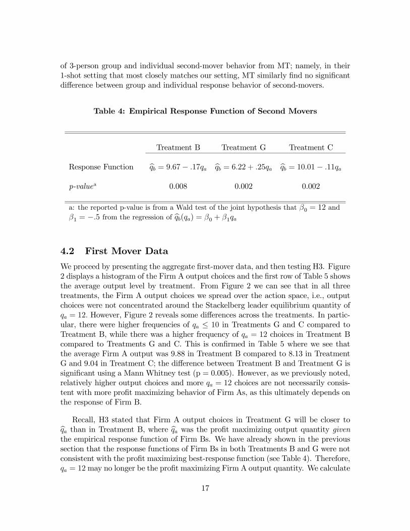
To help quantify this, we estimate the empirical response function, which we de-note bqb(qa), via a simple linear regression of the observed second-mover�s responsequantity on the �rst-movers quantity and a constant, i.e., bqb(qa) = �0 + �1qa. Ta-ble 4 presents the results. Given the parameterization of the Stackelberg duopoly weconsider, the theoretical best-response function is given by: qBRb (qa) = 12� :5qa: How-ever, from Table 4, we can see that bqb(qa) 6= qBRb (qa) for each of the three treatments.Speci�cally, using a Wald test, we can reject the null hypotheses that �0 = 12 and�1 = �:5 at the 1% level for each of the three treatments, which further con�rms thepattern observed in Figure 1 that the empirical response functions are �atter thanpro�t maximizing best-response function.

To summarize, the data reveals that subjects playing the role of Firm B exhibitedresponse decisions that was largely inconsistent with pro�t maximizing behavior, re-gardless of the treatment. In particular, Firm Bs best responded less than 50% of thetime, and their estimated response functions did not coincide with the pro�t maxi-mizing best-response function. In addition. the data revealed very little di¤erence inthe response data from Firm Bs in Treatment B compared to Firm Bs in TreatmentG or Treatment C. Hence, the data fails to support H1 and H2 that group decisionmaking units and a 10-minute cooling-o¤ period will lead to Stackelberg follower de-cisions that are more in line with pro�t maximization. Our comparison of 2-persongroup and individual second-mover behavior is largely consistent with the comparison

16

of 3-person group and individual second-mover behavior from MT; namely, in their1-shot setting that most closely matches our setting, MT similarly �nd no signi�cantdi¤erence between group and individual response behavior of second-movers.

Table 4: Empirical Response Function of Second Movers

Treatment B Treatment G Treatment C

Response Function bqb = 9:67� :17qa bqb = 6:22 + :25qa bqb = 10:01� :11qap-valuea 0.008 0.002 0.002

a: the reported p-value is from a Wald test of the joint hypothesis that �0 = 12 and�1 = �:5 from the regression of bqb(qa) = �0 + �1qa

4.2 First Mover Data

We proceed by presenting the aggregate �rst-mover data, and then testing H3. Figure2 displays a histogram of the Firm A output choices and the �rst row of Table 5 showsthe average output level by treatment. From Figure 2 we can see that in all threetreatments, the Firm A output choices we spread over the action space, i.e., outputchoices were not concentrated around the Stackelberg leader equilibrium quantity ofqa = 12: However, Figure 2 reveals some di¤erences across the treatments. In partic-ular, there were higher frequencies of qa � 10 in Treatments G and C compared toTreatment B, while there was a higher frequency of qa = 12 choices in Treatment Bcompared to Treatments G and C. This is con�rmed in Table 5 where we see thatthe average Firm A output was 9.88 in Treatment B compared to 8.13 in TreatmentG and 9.04 in Treatment C; the di¤erence between Treatment B and Treatment G issigni�cant using a Mann Whitney test (p = 0.005). However, as we previously noted,relatively higher output choices and more qa = 12 choices are not necessarily consis-tent with more pro�t maximizing behavior of Firm As, as this ultimately depends onthe response of Firm B.

Recall, H3 stated that Firm A output choices in Treatment G will be closer tobqa than in Treatment B, where bqa was the pro�t maximizing output quantity giventhe empirical response function of Firm Bs. We have already shown in the previoussection that the response functions of Firm Bs in both Treatments B and G were notconsistent with the pro�t maximizing best-response function (see Table 4). Therefore,qa = 12may no longer be the pro�t maximizing Firm A output quantity. We calculate

17

bqa for each treatment, given the empirical response functions of Firm B in Table 4,which are shown in the second row of Table 5. From Table 5, we can see thatchoosing bqa = 7:83, bqa = 7:90, and bqa = 7:41 is optimal for �rst-movers, given bqb(qa);in Treatment B, Treatment G, and Treatment C, respectively.

Figure 2: First-Mover Output Choices

Table 5: First Movers (FM) Output Data: All Treatments

Treatment B Treatment G Treatment C

Avg Output (qa) 9.88 8.13*** 9.04

bqa j bqb(qa) 7.83 7.90 7.41

Abs Dev from bqa 2.41 1.45*** 1.95

Notes: Avg Output and Abs Dev from bqa were tested using a Mann-WhitneyU-test, in relation to Treatment B***denotes signi�cance at the 1% level

18

Similar to testing H1 and H2, we test H3 using the absolute deviation from bqa,denoted Abs Dev from bqa; which measures how far away the Firm A output choiceswere away from the conditional pro�t maximizing output level. The third row ofTable 5 presents the average Abs Dev from bqa for each of the three treatments.From Table 5, we can see that the average Abs Dev from bqa is 1.45 in Treatment Gcompared to 2.41 in Treatment B. This di¤erence is signi�cant at the 1% level usinga Mann-Whitney Test (p = 0.004). Thus, the data provides support for H3, namely,�rst-movers in Treatment G choose output levels that are closer to the conditionalpro�t maximizing output level, relative to �rst-movers in Treatment B.

To summarize, the data reveals that groups acting as Firm As choose signi�cantlylower output levels than individuals acting as Firm As. However, after conditioning onthe actual aggregate empirical response function of Firm Bs, the group Firm As chooseoutput levels that are signi�cantly closer to the conditional pro�t maximizing outputlevel than individual Firm As. Hence, the data generally supports out hypothesis(H3) that group �rst-movers exhibit Stackelberg behavior that is more consistentwith pro�t maximization. Our comparison of 2-person group and individual �rst-mover output choices di¤ers somewhat from the comparison of 3-person groups andindividuals in MT; namely, in their 1-shot setting that most closely matches oursetting, MT �nd that average group �rst-mover choices of 9.33 and di¤erent from theaverage individual �rst-mover choices of 9.11.

5 Conclusion

The previous experimental tests of the Stackelberg duopoly model have found littlesupport for the Subgame Perfect equilibrium predictions of the model (HMN andHW). We hypothesize that the theoretically inconsistent results from HMN and HWare a result of systematic di¤erences between the lab environments used and naturallyoccurring �rm environments. Additionally, these di¤erences in the decision makingenvironments may limit the generalizability of the lab results from HMN and HWto �rm behavior in the �eld. The motivation of the study is twofold. First, thisstudy experimentally investigates whether unitary decision making groups exhibitmore pro�t maximizing Stackelberg behavior than individuals. Second, this studyexperimentally investigates whether a cooling-o¤ period leads second-movers to makedecisions that are more in line with the predicted pro�t maximizing best-response. Weargue that group decision making units and cooling-o¤periods are both representativeof decision-making units in the �eld, hence, our motivation to investigate their impacton decision making in an experimental Stackelberg duopoly in the lab.

In relation to the in�uence of group decision making, the data reveals very littledi¤erence in the decision making of second-movers between individuals and 2-personunitary groups. Speci�cally, both group and individual second-movers exhibit behav-

19

ior that is inconsistent with pro�t maximizing best-response. However, group �rst-movers choose output levels that are signi�cantly lower than individual �rst-movers.Initially, one might think that this pattern in the data reveals that group �rst-moversare exhibiting behavior that in more inconsistent with pro�t maximization. However,after conditioning on the empirical non best-response of second-movers, the data re-veals that the chosen output levels of group �rst-movers are signi�cantly closer tothe predicted pro�t maximizing quantity than individual �rst-movers. Additionally,total duopoly pro�ts are signi�cantly larger in the markets where 2-person groupsacts as �rms compared to individuals.

Note, group �rst-movers choosing quantity levels that are lower than the pre-dicted Stackelberg leader quantity (qa = 12) is consistent with the idea that group�rst-movers exhibited more �clever�decision making by collectively correctly antic-ipated the non best-response of second-movers and, consequently, maximized pro�tsby choosing lower quantity levels, relative to individual �rst-movers. However, analternative explanation is that group �rst-movers where simply exhibiting more co-operative behavior, which would also correspond to choosing lower quantities. Groupsexhibiting more cooperative behavior would be consistent with the �ndings of Casonand Mui (1997), and what they refer to as the �Social Comparison Theory�(SCT).The idea is that group members want to be perceived in a socially desirable way byother group members and, as a result, group decision making is more cooperative.However, this is contrast with the �social support of self-interested competitiveness�and the �schema-based distrust�hypotheses that predict more competitive behaviorby groups. Given the body of experimental literature (discussed in Section 2) that gen-erally �nds more competitive and self-interested behavior by groups, we are inclinedto think that the former is the more plausible explanation, i.e., group �rst-moversappear to exhibit behavior that is more consistent with rational pro�t maximization.

In relation to the a¤ect of a cooling-o¤periods, the data reveals that the 10-minutecooling-o¤ period did not lead to signi�cantly di¤erent second-mover response deci-sions, relative to when there was no cooling-o¤ period. In particular, second-moverswith and without the cooling-o¤period exhibited behavior that was inconsistent withthe predicted pro�t maximizing best-response. In fact, second-movers that had the10-minute cooling-o¤ period actually choose response quantities that were furtherfrom the best-response output level, although these di¤erences were not signi�cantat standard levels. One possibility is that the �cooling-o¤�period may have actuallyacted as more of a �heating-up�period for harboring emotions, rather than cooling-o¤emotions as it was intended to do.

We acknowledge that the observed lack of e¤ectiveness of the cooling-o¤ period,in the sense that it did not lead to more rational pro�t maximizing best responses,may be a by-product of the chosen length, 10 minutes. However, Grimm and Mengel(2011) found evidence that a 10-minute cooling-o¤ period was long enough to have

20

an e¤ect on response behavior in an ultimatum game. Additionally, to the best of ourknowledge, the literature related to the e¤ect of cooling-o¤periods does not postulateany formal model linking the length of the cooling-o¤period to its e¤ectiveness. Thus,there is no reason to suspect, a priori, that a longer cooling-o¤ period would producedi¤erent results. Additionally, using a longer cooling-o¤ period, e.g. 24-hours, wouldbe cumbersome and impractical to implement in a lab, thus undermining one of ourinitial motivations to use a 10-minute cooling-o¤ period. Certainly, future researchthat investigates the e¤ectiveness of cooling-o¤ periods, with respect to duration andthe context of the decision making environment, is warranted.

By investigating the impact of group decision making and cooling-o¤ periods in aStackelberg game, this study contributes to the mature body of literature on groupdecision making and growing body of literature on cooling-o¤ periods. Overall, we�nd that unitary groups earn higher pro�ts, and that group �rst-movers in the Stack-elberg game exhibit decision making that is more consistent with rational pro�t max-imization, which suggests that group decision making might foster collective criticalthought and more clever decision making in games. Whereas, we �nd that groupsecond-movers exhibit decision making similar to individuals, which suggests thatgroups decision making may be less e¤ective at mitigating the in�uence of non-sel�shmotivations. Additionally, a 10-minute cooling-o¤ period did not result in second-mover decisions that were more consistent with pro�t maximization. As a broadermethodological contribution, we hope the results of this study can provide insightsregarding the design of future lab experiments that seek to investigate behavior inmodels of �rm decision making. In particular, when testing models that require rel-atively higher levels of critical thought and strategic sophistication, implementinggroup decision making in the lab might result in behavior that is more consistentwith pro�t maximization. However, when testing models where social preferencesand emotional motivations are likely to be salient, implementing a protocol that fea-tures group decision making or a short cooling-o¤ period might have little e¤ect onbehavior in the lab.

21

6 Appendix

6.1 Player Instructions - Baseline Treatment14

PLAYER INSTRUCTIONS

Welcome to our experiments! Please read these instructions carefully! Do not talkto your neighbors and please remain quiet during the entire experiment. Raise yourhand if you have a question. We will answer them privately. In our experiment, youcan earn di¤erent amounts of money, depending on your decisions and the decisionof the other participants who are matched with you.You play the role of a �rm which produces the same product as another �rm in

the market. Both �rms always have to make a single decision, namely the amount ofoutput they want to produce in this market. The pro�t to each �rm will depend onthe level of output chosen by each of the �rms. In the table on the other sheet that isgiven to you, you can see the pro�ts of each �rm for all possible output combinationsof the two �rms. The table reads as follows: the header of the row represents one�rm�s output decision (Firm-A) and the header of the column represents the outputdecision of the other �rm (Firm-B). Inside the little box where row and columnintersect, Firm-A�s pro�t corresponding to this combination of outputs is the numberto the left. Firm-B�s pro�t corresponding to this combination of outputs is the numberto the right. The pro�t is denoted in a �ctitious unit of money which we call Taler.Before the experiment begins, you will have a few minutes to look over the payo¤table. You will then be asked two control questions about the matrix to ensure yourunderstanding of it.You have been randomly assigned either the role of Firm-A or Firm-B, and ran-

domly matched to another participant of the opposite role. After the two controlquestions, your Firm role will be revealed to you. The experiment will proceed inthree stages.

Stage 1: Firm-A will begin by choosing an output level to produce. Firm-A�s outputlevel will then be revealed to Firm-B.

Stage 2: Firm-B will then respond by choosing an output level to produce.

Stage 3: The output decisions of both Firms and the corresponding pro�ts of eachFirm will be displayed to both Firms. You will then be asked to complete asimple questionnaire that will take approximately 10 minutes to complete.

14The instructions for the Group Treatment were essentially identical to the Baseline Treatment.Except, subjects were informed that they, along with another subject, comprise a two person groupthat will be playing the role of a �rm.

22

After all three stages are complete; you will be privately paid your experimentalearnings. Your pro�t in Talers from the decision task will be converted to $ at a rateof 10-1. That is, every 10 Talers correspond to $1 USD. In addition to your pro�t,you will receive a $3 USD show-up payment for participating in the experiment.All decisions and answers to the questionnaire will be kept anonymous among theparticipants and the experimenters.

6.2 Player Instructions - Cooling-o¤ Treatment

PLAYER INSTRUCTIONS

Welcome to our experiments! Please read these instructions carefully! Do not talkto your neighbors and please remain quiet during the entire experiment. Raise yourhand if you have a question. We will answer them privately. In our experiment, youcan earn di¤erent amounts of money, depending on your decisions and the decisionof the other participants who are matched with you.You play the role of a �rm which produces the same product as another �rm in

the market. Both �rms always have to make a single decision, namely the amount ofoutput they want to produce in this market. The pro�t to each �rm will depend onthe level of output chosen by each of the �rms. In the table on the other sheet that isgiven to you, you can see the pro�ts of each �rm for all possible output combinationsof the two �rms. The table reads as follows: the header of the row represents one�rm�s output decision (Firm-A) and the header of the column represents the outputdecision of the other �rm (Firm-B). Inside the little box where row and columnintersect, Firm-A�s pro�t corresponding to this combination of outputs is the numberto the left. Firm-B�s pro�t corresponding to this combination of outputs is the numberto the right. The pro�t is denoted in a �ctitious unit of money which we call Taler.Before the experiment begins, you will have a few minutes to look over the payo¤table. You will then be asked two control questions about the matrix to ensure yourunderstanding of it.You have been randomly assigned either the role of Firm-A or Firm-B, and ran-

domly matched to another participant of the opposite role. After the two controlquestions, your Firm role will be revealed to you. The experiment will proceed inthree stages.

Stage 1: Firm-A will begin by choosing an output level to produce. Firm-A�s outputlevel will then be revealed to Firm-B.

Stage 2: Both Firms will then be asked to complete a simple questionnaire that willtake approximately 10 minutes to complete.

Stage 3: After the questionnaire, Firm-B will then respond by choosing an outputlevel to produce. Then output decisions of both Firms and the correspondingpro�ts of each Firm will be displayed to both Firms.

23

After all three stages are complete; you will be privately paid your experimentalearnings. Your pro�t in Talers from the decision task will be converted to $ at a rateof 10-1. That is, every 10 Talers correspond to $1 USD. In addition to your pro�t,you will receive a $3 USD show-up payment for participating in the experiment.All decisions and answers to the questionnaire will be kept anonymous among theparticipants and the experimenters.

6.3 Questionnaire

1. What is your gender?

2. How old are you?

3. What is your class level?

4. What is your major?

5. What is your approximate GPA?

6. Have you ever taken an economics course?

7. Are you currently employed?

8. Is your current job in a business related industry?

9. How many total years of work experience do you have?

10. Have you ever participated in an experiment?

11. How did you hear about the Economic Science Lab?

12. Have you ever referred a friend to the Economic Science Lab?

13. Is English your �rst language?

14. Are you an Arizona resident?

15. Are you currently carrying more than $10 in cash?

16. Suppose a bat and a ball cost a total of $1.10, and the bat cost $1.00 more thanthe ball. How much does the ball cost? (Frederick 2005; CRT #1)

17. Suppose it takes 5 machines 5 minutes to make 5 gadgets. How many minutesdoes it take for 100 machines to make 100 gadgets? (Frederick 2005; CRT #2)

18. In a lake, there is a patch of lillypads. Everyday the patch doubles in size. Ittakes 48 days for the patch to cover the entire lake. How many days does ittake to cover 1/2 of the lake? (Frederick 2005; CRT #3)

24

References

[1] Adler, R., Rosen. B., & Silverstein, E. (1998). �Emotions in Negotiation: HowTo Manage Fear and Anger.�Negotiation Journal 14, 161-179.

[2] Bornstein, G., Kugler, T. & Ziegelmeyer, A. (2004). �Individual and group de-cisions in the centipede game: are groups more �rational�players?� Journal ofExperimental Social Psychology 40, 599-605.

[3] Bornstein, G. (2008). A Classi�cation of Games by Player Type. In A. Biel, D.Eek, T. Gärling, & M. Gustafsson (Eds.), New Issues and Paradigms in Researchon Social Dilemmas, pp. 27-42. New York: Springer.

[4] Bornstein, G. & Yaniv, I. (1998). �Individual and group behavior in the ulti-matum game: are groups more �rational�players?�Experimental Economics 1,101-108.

[5] Brown, R. (1954). Mass phenomena. In G. Lindzey (Ed.), Handbook of SocialPsychology, pp. 833-876. Cambridge, MA: Addison- Wesley.

[6] Campbell, D. T., & Stanley J.C. (1963). Experimental and Quasi-ExperimentalDesigns for Research. Boston: Houghton Mi­ in.

[7] Cason, T. & Mui, V. (1997). �A laboratory study of group polarization in theteam dictator game.�Economic Journal 107, 1465-1483.

[8] Charness, G., & Rabin, M. (2002). �Understanding Social Preferences with Sim-ple Tests.�The Quarterly Journal of Economics 117, 817-869.

[9] Cooper, D. & Kagel, J. (2005). �Are two heads better than one? Team versusindividual play in signaling games.�American Economic Review 95, 477-509.

[10] Cox, J. (2002). �Trust, reciprocity, and other-regarding preferences: groups vs.individuals and males vs. females.�In R. Zwick & A. Rapoport (Eds.), Advancesin experimental business research, pp. 331-350. Dordrecht: Kluwer AcademicPublishers.

[11] Cox, J., and Hayne, S. (2006). �Barking up the Right Tree: Are Small GroupsRational Agents?�Experimental Economics 3, 209-222.

[12] Dufwenberg, M. & Kirchsteiger, G. (2004). �A Theory of Sequential Reciprocity.�Games and Economic Behavior 47, 268-298.

[13] Dufwenberg, M., Smith, A., & Van Essen, M. (forthcoming). �Hold-up: With aVengeance.�Economic Inquiry.

25

[14] Falk, A., Heckman, J. (2009). �Lab Experiments are a Major Source of Knowl-edge in the Social Sciences.�Science 326, 535-538.

[15] Fehr, E. & Schmidt, K. (1999). �A Theory of Fairness, Competition, and Coop-eration.�The Quarterly Journal of Economics 114, 817-868.

[16] Fischbacher, U. (2007). �z-Tree, Toolbox for Readymade Economic Experi-ments.�Experimental Economics 10, 171-178.

[17] Fonseca, M., Huck, S. & Normann, H. (2005). �Playing Cournot AlthoughShouldn�t: Endogenous Timing in Experimental Duopolies with AsymmetricCosts.�Economic Theory 25, 669-677.

[18] Fonseca, M., Muller, W. & Normann, H. (2006). �Endogenous Timing inDuopoly: Experimental Evidence.� International Journal of Game Theory 34,443-456.

[19] Frederick, S. (2005). �Cognitive Re�ection and Decision Making.� Journal ofEconomic Perspectives 19, 25-42.

[20] Friedman, D., & Sunder, S. (1994). �Experimental Methods: A Primer for Econo-mists.�Cambridge University Press.

[21] Gneezy, U., & List, J. (2006). �Putting Behavioral Economics to Work: Testingfor Gift Exchange in Labor Markets Using Field Experiments.� Econometrica74, 1365-1384.

[22] Goleman, D. (1995). Emotional intelligence. New York: Bantam Books.

[23] Grimm, V., & Mengel, F. (2011). �Let Me Sleep on it: Delay Reduces RejectionRates in Ultimatum Games.�Economic Letters 111, 113-115.

[24] Hamilton, J. & Slutsky, S. (1990). �Endogenous Timing in Duopoly Games:Stackelberg or Cournot Equilibria.�Games and Economic Behavior 2, 29-46.

[25] Harrison, G. & List, J. (2004). �Field Experiments.�Journal of Economic Liter-ature 42, 1009-1055.

[26] Huck, S., Muller, W. & Normann, H. (2001). �Stackelberg Beats Cournot: OnCollusion and E¢ ciency in Experimental Markets.�The Economic Journal 111,749-765.

[27] Huck, S., Muller, W. & Normann, H. (2002). �To Commit or Not to Commit:Endogenous Timing in Experimental Duopoly Markets.�Games and EconomicBehavior 38, 240-264.

26

[28] Huck, S. & Wallace, B. (2002). �Reciprocal Strategies and Aspiration Levels ina Cournot-Stackelberg Experiment.�Economics Bulletin 3, 1-7.

[29] Insko, C., & Schopler, J. (1987). Categorization, competition and collectivity. InC. Hendrick (Ed.), Group processes. Vol. 8, pp. 213-251. New York: Sage.

[30] Insko, C., Hoyle, R., Pinkley, R., Hong, G., Slim, R., Dalton, G., Lin, Y., Ru¢ n,P., Dardis, G., Berthal, P., & Schopler, J. (1988). �Individual-group discontinu-ity: The role of a consensus rule.� Journal of Experimental Social Psychology24, 505-19.

[31] Insko, C. A., Schopler, J., Hoyle, R., Dardis, G., & Graetz, K. (1990).�Individual-group discontinuity as a function of fear and greed.�Journal of Per-sonality and Social Psychology 58, 68-79.

[32] Insko, C., Schopler, J., Graetz, K., Drigotas, S., Currey, D., Smith, S., Brazil, D.,& Bornstein, G. (1994). �Interindividual-Intergroup Discontinuity in Prisoner�sDilemma Game.�The Journal of Con�ict Resolution 38, 87-116.

[33] Kahneman, D. (2003). �Perspective on Judgment and Choice: Mapping BoundedRationality.�American Psychologist 58, 697-720.

[34] Kocher, M. G., & Sutter, M. (2005). �The decision maker matters: individualversus group behavior in experimental beauty-contest games.�Economic Journal115, 200�223.

[35] Kugler, T., Bornstein, G., Kocher, M. G., & Sutter, M. (2007). �Trust betweenindividuals and groups: groups are less trusting than individuals but just astrustworthy.�Journal of Economic Psychology 28, 646-657.

[36] Kugler, T., Kausel, E., & Kocher M. (2012). �Are Groups more Rational than In-dividuals? A Review of Interactive Decision Making in Groups.�CESifo WorkingPaper.

[37] Lau, S. & Leung, F. (2010). �Estimating a Parsimonious Model of InequalityAversion in Stackelberg Duopoly Experiments.�Oxford Bulletin of Economicsand Statistics 72, 669-686.

[38] Levitt, S., & List, J. (2007). �What do Laboratory Experiments Measuring SocialPreferences Reveal About the Real World.�Journal of Economic Perspectives 21,153-174.

[39] Loewenstein, G. (2000). �Emotions in Economic Theory and Economic Behav-ior.�The American Economic Review 90, 426-432.

[40] Luhan, W., Kocher, M., & Sutter, M. (2009). �Group Polarization in the TeamDictator Game Reconsidered.�Experimental Economics 12, 26-41.

27

[41] McCallum, D. M., Harring, K., Gilmore, R., Drenan, S., Chase, J., Insko, C. A.,& Thibaut, J. (1985). �Competition Between Groups and Between Individuals.�Journal of Experimental Social Psychology 21, 301-320.

[42] Messick, D., Moore, D., & Bazerman, M. (1997). �Ultimatum Bargaining with aGroup: Underestimating the Importance of the Decision Rule.�OrganizationalBehavior and Human Decision Processes 69, 87-101.

[43] Normann, H-T., Ru­ e, B. (2011). �Introduction to the Special Issue on Experi-ments in Industrial Organization.�International Journal of Industrial Organiza-tion 29, 1-3.

[44] Oechssler, J., Roider, A., & Schmitz, P. (2008). �Cooling-O¤ in Negotiations �Does it Work?�Working paper.

[45] Robert, C., & Carnevale, P. (1997). �Group Choice in Ultimatum Bargaining.�Organizational Behavior and Human Decision Processes 72, 256-279.

[46] Sanfey, A., Rilling, J., Aronson, J., Nystrom, L., & Cohen, J. (2003). �TheNeural Basis of Economic Decision-Making in the Ultimatum Game.� Science300, 1755-1758.

[47] Schopler, J., Insko, C., Graetz, K., Drigotas, S., & Smith, V. (1991). �TheGenerality of the Individual-group Discontinuity E¤ect: Variations in Positivity-negativity of Outcomes, Players�Relative Power, and Magnitude of Outcomes.�Personality and Social Psychology Bulletin 17, 612-24.

[48] Schopler, J., Insko, C., Graetz, K., Drigotas, S., Smith, V., & Dahl, K. (1993).�Individual-group Discontinuity: Further Evidence for Mediation by Fear andGreed.�Personality and Social Psychology Bulletin 19, 419-31.

[49] Smith, V.L. (1982). �Microeconomic Systems as an Experimental Science.�TheAmerican Economic Review 72, pp. 923-955

[50] Sutter, M. (2005). �Are four heads better than two? An experimental beauty-contest game with teams of di¤erent size.�Economic Letters 88, 41-46.

[51] Ury, W., Brett, J., & Goldberg, S. (1988). �Designing and E¤ective DisputeResolution System.�Negotiation Journal 4, 413-431.

[52] Wilde, L. (1981). �On the use of Laboratory Experiments in Economics.�In P.Joseph (Ed.), The Philosophy of Economics, pp. 137-143. Dordrecht: Reidel.

28