Embed Size (px)
Citation preview

Derived Inputs: Applications ofPrincipal Components
-Applied Multivariate Analysis-
Lecturer: Darren Homrighausen, PhD
1

Lower Dimensional Embeddings: TurtleExample
This data set gives a morphological description of 48 turtles (thismeans, we get the height, weight, length, and gender of theturtles). What does the data look like?
length
80 90 100 110 120 130
● ●●
●●●●●●
●●●●●●
●● ●●●
●●●
●
●
●●●
●
● ●
● ● ●●●●●
●
●●●
●●● ●
●
●
100
120
140
160
180
●●●
●●● ●●●
●●●●●●
●● ●●●●●
●●
●
● ●●
●
●●
●●● ●● ●●
●
●●
●●●
●●●
●
8090
100
110
120
130
●
●●
●●
●●●●
●●●
●●●●
●
●●
●
●●●
●
●
●●●
●
●
●
●
●
●
●●
●●
●
●● ●
●●
●
●
●
●
width
●
●●
●●
●●●●
●●●
●●●●
●
●●
●
●●●
●
●
●●●
●
●
●
●
●
●
●●
●●
●
●●●
●●
●
●
●
●
100 120 140 160 180
●
●●
●●●
●●●
●●●
●
●●●●
●
●
●●●●
●
● ●
●
●
●
●
●
●●
●
●●
●●
●
●
●●
●
●
●●
●
●
●
●●
●●
●
●●●
●●
●
●
●●●●
●
●
● ●●●
●
● ●
●
●
●
●
●
● ●
●
●●
●●
●
●
●●
●
●
●●
●
●
35 40 45 50 55 60 6535
4045
5055
6065
height
2

Lower Dimensional Embeddings: TurtleExample
Actually, we can do better. Use this code:
library(ade4)
data(tortues)
pturtles = tortues #rename to a english word
names(pturtles) = c("length", "width", "height", "sex")
sex = pturtles$sex
sexcol = ifelse(sex == "F", "pink", "blue")
measures = pturtles[, 1:3]
#you need to install rgl using install.packages(’rgl’)
library(rgl)
plot3d(measures, type = "s", col = sexcol)
3

Lower Dimensional Embeddings: TurtleExample, Go to 3d Plot.
Some notes:
• Notice that our covariates vector has length 3.(Xi = (lengthi ,widthi ,heighti )
> ∈ R3)
• However, as length, width, and height are extremely (linearly)related, it can be argued that the data vector is actually only1 dimensional, plus some noise.
• So, maybe instead of trying to pick one of these variables, weshould use their shared 1 dimensional space.
4

Lower Dimensional Embeddings: TurtleExample
This data demonstrates the need for scaling
> measures
length width height
1 93 74 37
2 94 78 35
...
48 177 132 67
> scale(measures, center = TRUE, scale = TRUE)
length width height
1 -1.54712021 -1.69075466 -1.0908212
2 -1.49829590 -1.37619565 -1.3293607
...
48 2.55412153 2.87035093 2.4872711
5

Two common uses of PCA
Exploratory Data Analysis (EDA): Using the nature of theestimated rotation of our predictors to draw conclusions about howthe predictors are related to each other
Principal Components Regression (PCR): Use the principalcomponents as the inputs to a regression procedure to discoverrelationships between the predictors and the response
We’ll cover both of these, starting with EDA.
6

Using PCA for EDA
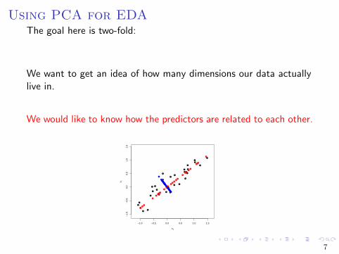
The goal here is two-fold:
We want to get an idea of how many dimensions our data actuallylive in.
We would like to know how the predictors are related to each other.
7

Using PCA for EDAThe goal here is two-fold:
We want to get an idea of how many dimensions our data actuallylive in.
We would like to know how the predictors are related to each other.
●
●
●
●
●
●
●
●
●
●
●
●
●
●
●
●
●
●
●
●
●●
●
●
●
●
●
●
●
●
−2 −1 0 1 2
−2
−1
01
2
x1
x 2 ● ●● ●●● ● ●●● ●● ●● ●● ●●● ● ●●●● ●● ●● ● ●●
●
●
●
●
●
●
●
●
●
●
●
●
●
●
●
●
●
●
●
●●
●
●
●
●
●
●
●
●
●
●
●
DataOnly x_1Only x_2
7
Using PCA for EDAThe goal here is two-fold:
We want to get an idea of how many dimensions our data actuallylive in.
We would like to know how the predictors are related to each other.
●
●
●
●
●
●
●
●
●
●
●
●
●
●
●
●
●
●
●
●
●
●
●
●
●
●
●
●
●
●
−1.0 −0.5 0.0 0.5 1.0 1.5
−1.
0−
0.5
0.0
0.5
1.0
1.5
x1
x 2
●
●
●
●
●
●
●
●
●
●
●
●
●
●
●
●●●
●
●
●●
●●
●
●
●
●
●
●
●●
●
●●●
●
●
●
●
●
●
●
●●
●
●
●
●●
●●
●
●
●
●●
●
●
●
●
●
DataPC1 only
7

Using PCA for EDA: How Many Dimensions?R Code
pc.shell = prcomp(measures,scale=TRUE)
pc.summary = summary(pc.shell)
> pc.summary
Importance of components:
PC1 PC2 PC3
Standard deviation 1.7073 0.2528 0.14611
Proportion of Variance 0.9716 0.0213 0.00712
Cumulative Proportion 0.9716 0.9929 1.00000
#Boxplot
plot(pc.shell,main=’Variance Explained’,xlab=’PCs’)
#scree plot
p = ncol(measures)
plot(0:p,c(1,1-pc.summary$importance[3,]),type="l",
xlab=’PCs’,ylab=’Cummulative Var Explained’,
main="Scree-plot",ylim=c(0,1))
points(1:p,c(1-pc.summary$importance[3,]))
8

Using PCA for EDA: How Many Dimensions?
PCA finds the rotation that maximizes variance
We can order the PCs by how much variance each one explains.
Then, we retain the PCs that explain “enough” variance
9
Using PCA for EDA: How Many Dimensions?
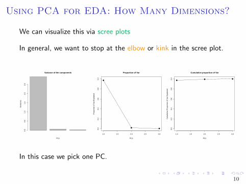
We can visualize this via scree plots
In general, we want to stop at the elbow or kink in the scree plot.
Variance of the components
PCs
Var
ianc
es
0.0
0.5
1.0
1.5
2.0
2.5
1.0 1.5 2.0 2.5 3.0
0.0
0.2
0.4
0.6
0.8
1.0
Proportion of Var
PCs
Pro
port
ion
of V
ar E
xpla
ined
●
●●
1.0 1.5 2.0 2.5 3.0
0.0
0.2
0.4
0.6
0.8
1.0
Cumulative proportion of Var
PCs
Cum
ulat
ive
Pro
port
ion
of V
ar E
xpla
ined
●● ●
In this case we pick one PC.
10

Using PCA for EDA: LoadingsWe can see how the covariates relate to each other via loadings(These are the coordinates of the covariates in the PCs)
> pc.shell$rotation
PC1 PC2 PC3
length 0.5806536 -0.2706983 0.7678306
width 0.5780575 -0.5270479 -0.6229526
height 0.5733158 0.8055699 -0.1495531
• PC1 is comprised of a roughly equal linear combination ofeach of the variables.
• PC2 has a large value of height and medium negative valuesfor length and width(This indicates that PC2 describes shells that are pointy)
• PC3 has a large value of length, medium negative value forwidth, and a negligible value for height.(This indicates that PC3 describes shells that are long and narrow)
11

Using PCA for EDA: Scores
We can see how the observations relate to each other via scores(These are the coordinates of the observations in the PCs)
> pc.shell$x
PC1 PC2 PC3
1 -2.501079256 0.431178792 0.0284694367
2 -2.427654498 0.060014223 -0.0943228042
3 -2.280037885 -0.049312926 -0.1173228864
4 -1.682937763 0.103136589 -0.1971828906
5 -1.677508679 -0.047607104 -0.1908457721
6 -1.899371091 0.008883803 0.0604355449
7 -1.643346040 0.104933543 -0.0357276551
8 -1.586646026 0.078500233 0.0392499421
9 -1.672133541 0.010650380 0.1435647400
...
48 4.568279372 -0.200538058 -0.1989389715
12
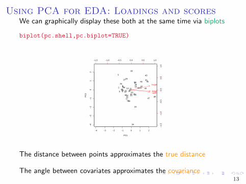
Using PCA for EDA: Loadings and scoresWe can graphically display these both at the same time via biplots
biplot(pc.shell,pc.biplot=TRUE)
−4 −3 −2 −1 0 1 2
−4
−3
−2
−1
01
2
PC1
PC
2
1
2
3
4
56
789
10
1112
13
1415
1617
18
19
20
212223
24
25
26
27
28
29
30
31
32
33
34
3536
3738
39
40
4142
43
44
4546
4748
−1.5 −1.0 −0.5 0.0 0.5 1.0
−1.
5−
1.0
−0.
50.
00.
51.
0
lengthwidth
height
The distance between points approximates the true distance
The angle between covariates approximates the covariance13

Using PCA for EDA: Dimensional reductionUsing the scree plot, we decided one dimension is all that isrequired to represent this data
Let’s plot that dimension in a univariate fashion and see how itrelates to the sex label
plot(pc.shell$x[,1],rep(0,nrow(pc.shell$x)))
●●● ●●● ●●● ●●● ●●●●● ●● ● ●●● ●
−2 −1 0 1 2 3 4
PC 1 scores
14

Digits example
15

Using PCA for EDA: Digits Example
Source: http://www-stat.stanford.edu/∼tibs/ElemStatLearn/
Our data is 658 handwritten 3’s, each drawn by a different person
Each image is 16x16 pixels, each taking grayscale values between-1 and 1.
16

Digits example: How does this fit withprevious examples?
Think about each pixel location as a measurement
Consider these simple drawings of 3’s. We convert this to anobservation in a matrix by unraveling it along rows
X1 =−0.2 0.0 0.2 0.4 0.6 0.8 1.0 1.2
0.0
0.2
0.4
0.6
0.8
1.0
X2 =−0.2 0.0 0.2 0.4 0.6 0.8 1.0 1.2
0.0
0.2
0.4
0.6
0.8
1.0
X1 = [1, 1, 1, 0, 0, 1, 0, 1, 1, 0, 0, 1, 1, 1, 1]>
X2 = [1, 1, 1, 0, 1, 1, 0, 0, 1, 0, 0, 1, 1, 1, 1]>
(Here, let black be 1 and white be 0)
17

Digits example
We will consider digits with...
• more pixels (p = 256)
• a continuum of intensities
Vs. −0.2 0.0 0.2 0.4 0.6 0.8 1.0 1.2
0.0
0.2
0.4
0.6
0.8
1.0
−0.2 0.0 0.2 0.4 0.6 0.8 1.0 1.2
0.0
0.2
0.4
0.6
0.8
1.0
18

Using PCA for EDA: Digits Example, Codefor Plotting Digits
plot.digit = function(x,zlim=c(-1,1)) {
cols = gray.colors(100)[100:1]
image(matrix(x,nrow=16)[,16:1],col=cols,
zlim=zlim,axes=FALSE)
}
19

Using PCA for EDA: Digits Example
Eventually, we will learn how to classify these digits. But, for now,let’s look at all 658 digits in principal components land.
load("../data/digits.Rdata")
threesCenter = scale(threes,scale=FALSE)
svd.out = svd(threesCenter)
pcs = svd.out$v
scores = svd.out$u%*%diag(svd.out$d)
Or, using prcomp:
out = prcomp(threes,scale=F)
pcs = out$rot
scores = out$x
(Note that here we aren’t scaling: the measurements are already on a consistent scale)
20

Using PCA for EDA: Digits ExampleWe can plot the scores of the first two principal components versuseach other:
plot(scores[,1],scores[,2],xlab = ’PC1’,ylab=’PC2’,
main=’Plot of First Two PCs’)
●●
●
●
●
●
●
●
● ●
●
●
●
●
●
●
●
●
●
●
●
●●
●
●
●
●
●●
●
●
●
●
●
●
●
●
●●
●
●
●
●
●
●
●
●
●
●●
●
●
●
●
●
●
●
●
●
●
●
●
●
●
●
●
●
●
●
●
●
●
●
●
●
●
●
●●
●
●
●
●
●
●●
●
●
●
●
●
●
●
●
●
●
●
●
●
●
●
●
●
●
●
●
●
●
●
●
●
●
●
●
●
●
●
●
●
●
●
●
●
●
●
●
●●
●
●
●
●
●
●
●
●
●
●
●
●
●
●
●
●
●
●
●
●
●
●
●
●
●
●●
●
●
●●
●
●
●
●
●
●
●
●
●
●●
●
●
●●
●
●
●
●
●
●
●
●
●
●
●
●
● ●
●
●
●
●●
●
●
●
●
●●
●
●
●
●
●
●
●
●
●
●
●
●
● ●
●
●●
●
●
●
●
●
●
●
●
●
●
●
●
●
●
●
●●
●
●
●
●
●
● ●
●
●
●
●
● ●
●●
●
●
●
●
●
●
●
●
●
●
● ●
●
●
●
●
●
●
●
●
●
●
●
●
●
●
●
●
●●
●
●
●
●
●
●
●
●●
●
●
●
●
●
●
●
●
●
●
●
●
●
●
● ●
●
●
●●
●
●
●
●
●
●
●
●●
●
●
●●
●
●
●●
●
●
●
●
●
●
●●
●
●
●
●
●
●
●
●
●●
●
●
●
●
●
●
●
●●
●
●
●
●
●
●
●
●
●
●
●●
●
●
●
●
●
●
●
●
●
●
●
●
●
●
●
●
●●
●
●
●●
●
●
●
●
●●
●
●
●
●
●
●
●
●
●
●
●
●
●
●
●
●
●
●
●
●
●
●
●
●
●
●
●
●
●●
●
●
●●
●
●
●
●
●
●
●●●
●
●
●
●
●
●
●
●
●
●
●
●
●
●
●
●
●●
●
●
●
●
●
●
●
●
●
●
●
●
●
●
●
●
●
●
●
●
●
●
●
●
●
●
●
●
●
●
●
●
●
●
●
●
●
●
●
●
●
●
●
●
●
●
●
●
●
●
●
●
●
●
●
●●
●
●
●
●
●●
●
●●
●
●● ●
●●
●●
●
●
●●
●
●
● ●
●
●
●
●
●
●
●
●
●
●
●
●
●
●
●
●
●
●
●
●
●
●
●
●
●●
●
●
●
●
●
●
●
●
●
●
●
●●
●
●
●
●
●
●
●
●
●
●
●●
●
●
●
●
●
●
●
●
● ●
●
●
●
●
●
●
●
●
●
●
●
●
● ●
●●
●
●
●
●
●
●
●
●
●
●
●
●
●
●
●
●●
●
●
●●
●
●
●
●
●
●
●
●
●
●
●
●
●
●
●
●●
●
●
●
●
●
●
●
●
●
−5 0 5
−6
−4
−2
02
46
Plot of First Two PCs
PC1
PC
2
Note: Each circle in this plot represents a hand written ‘3’.
21

Using PCA for EDA: Digits ExampleThe idea is that where a handwritten ‘3’ falls in the plot could berelated to some fundamental, underlying property.
In the turtle example, any shell that had a large value in PC2 hada tall and narrow shell.
Can we characterize the same thing about 3’s?
●●
●
●
●
●
●
●
● ●
●
●
●
●
●
●
●
●
●
●
●
●●
●
●
●
●
●●
●
●
●
●
●
●
●
●
●●
●
●
●
●
●
●
●
●
●
●●
●
●
●
●
●
●
●
●
●
●
●
●
●
●
●
●
●
●
●
●
●
●
●
●
●
●
●
●●
●
●
●
●
●
●●
●
●
●
●
●
●
●
●
●
●
●
●
●
●
●
●
●
●
●
●
●
●
●
●
●
●
●
●
●
●
●
●
●
●
●
●
●
●
●
●
●●
●
●
●
●
●
●
●
●
●
●
●
●
●
●
●
●
●
●
●
●
●
●
●
●
●
●●
●
●
●●
●
●
●
●
●
●
●
●
●
●●
●
●
●●
●
●
●
●
●
●
●
●
●
●
●
●
● ●
●
●
●
●●
●
●
●
●
●●
●
●
●
●
●
●
●
●
●
●
●
●
● ●
●
●●
●
●
●
●
●
●
●
●
●
●
●
●
●
●
●
●●
●
●
●
●
●
● ●
●
●
●
●
● ●
●●
●
●
●
●
●
●
●
●
●
●
● ●
●
●
●
●
●
●
●
●
●
●
●
●
●
●
●
●
●●
●
●
●
●
●
●
●
●●
●
●
●
●
●
●
●
●
●
●
●
●
●
●
● ●
●
●
●●
●
●
●
●
●
●
●
●●
●
●
●●
●
●
●●
●
●
●
●
●
●
●●
●
●
●
●
●
●
●
●
●●
●
●
●
●
●
●
●
●●
●
●
●
●
●
●
●
●
●
●
●●
●
●
●
●
●
●
●
●
●
●
●
●
●
●
●
●
●●
●
●
●●
●
●
●
●
●●
●
●
●
●
●
●
●
●
●
●
●
●
●
●
●
●
●
●
●
●
●
●
●
●
●
●
●
●
●●
●
●
●●
●
●
●
●
●
●
●●●
●
●
●
●
●
●
●
●
●
●
●
●
●
●
●
●
●●
●
●
●
●
●
●
●
●
●
●
●
●
●
●
●
●
●
●
●
●
●
●
●
●
●
●
●
●
●
●
●
●
●
●
●
●
●
●
●
●
●
●
●
●
●
●
●
●
●
●
●
●
●
●
●
●●
●
●
●
●
●●
●
●●
●
●● ●
●●
●●
●
●
●●
●
●
● ●
●
●
●
●
●
●
●
●
●
●
●
●
●
●
●
●
●
●
●
●
●
●
●
●
●●
●
●
●
●
●
●
●
●
●
●
●
●●
●
●
●
●
●
●
●
●
●
●
●●
●
●
●
●
●
●
●
●
● ●
●
●
●
●
●
●
●
●
●
●
●
●
● ●
●●
●
●
●
●
●
●
●
●
●
●
●
●
●
●
●
●●
●
●
●●
●
●
●
●
●
●
●
●
●
●
●
●
●
●
●
●●
●
●
●
●
●
●
●
●
●
−5 0 5
−6
−4
−2
02
46
Plot of First Two PCs
PC1
PC
2
Note: Each circle in this plot represents a hand written ‘3’. 22

Using PCA for EDA: Digits Example
quantile.vec = c(0.05,0.25,0.5,0.75,0.95)
quant.score1 = quantile(scores[,1],quantile.vec)
quant.score2 = quantile(scores[,2],quantile.vec)
plot(scores[,1],scores[,2],xlab = ’PC1’,ylab=’PC2’)
for(i in 1:5){
abline(h = quant.score2[i])
abline(v = quant.score1[i])
}
identify(scores[,1],scores[,2],n=25) #to find points
●●
●
●
●
●
●
●
● ●
●
●
●
●
●
●
●
●
●
●
●
●●
●
●
●
●
●●
●
●
●
●
●
●
●
●
●●
●
●
●
●
●
●
●
●
●
●●
●
●
●
●
●
●
●
●
●
●
●
●
●
●
●
●
●
●
●
●
●
●
●
●
●
●
●
●●
●
●
●
●
●
●●
●
●
●
●
●
●
●
●
●
●
●
●
●
●
●
●
●
●
●
●
●
●
●
●
●
●
●
●
●
●
●
●
●
●
●
●
●
●
●
●
●●
●
●
●
●
●
●
●
●
●
●
●
●
●
●
●
●
●
●
●
●
●
●
●
●
●
●●
●
●
●●
●
●
●
●
●
●
●
●
●
●●
●
●
●●
●
●
●
●
●
●
●
●
●
●
●
●
● ●
●
●
●
●●
●
●
●
●
●●
●
●
●
●
●
●
●
●
●
●
●
●
● ●
●
●●
●
●
●
●
●
●
●
●
●
●
●
●
●
●
●
●●
●
●
●
●
●
● ●
●
●
●
●
● ●
●●
●
●
●
●
●
●
●
●
●
●
● ●
●
●
●
●
●
●
●
●
●
●
●
●
●
●
●
●
●●
●
●
●
●
●
●
●
●●
●
●
●
●
●
●
●
●
●
●
●
●
●
●
● ●
●
●
●●
●
●
●
●
●
●
●
●●
●
●
●●
●
●
●●
●
●
●
●
●
●
●●
●
●
●
●
●
●
●
●
●●
●
●
●
●
●
●
●
●●
●
●
●
●
●
●
●
●
●
●
●●
●
●
●
●
●
●
●
●
●
●
●
●
●
●
●
●
●●
●
●
●●
●
●
●
●
●●
●
●
●
●
●
●
●
●
●
●
●
●
●
●
●
●
●
●
●
●
●
●
●
●
●
●
●
●
●●
●
●
●●
●
●
●
●
●
●
●●●
●
●
●
●
●
●
●
●
●
●
●
●
●
●
●
●
●●
●
●
●
●
●
●
●
●
●
●
●
●
●
●
●
●
●
●
●
●
●
●
●
●
●
●
●
●
●
●
●
●
●
●
●
●
●
●
●
●
●
●
●
●
●
●
●
●
●
●
●
●
●
●
●
●●
●
●
●
●
●●
●
●●
●
●● ●
●●
●●
●
●
●●
●
●
● ●
●
●
●
●
●
●
●
●
●
●
●
●
●
●
●
●
●
●
●
●
●
●
●
●
●●
●
●
●
●
●
●
●
●
●
●
●
●●
●
●
●
●
●
●
●
●
●
●
●●
●
●
●
●
●
●
●
●
● ●
●
●
●
●
●
●
●
●
●
●
●
●
● ●
●●
●
●
●
●
●
●
●
●
●
●
●
●
●
●
●
●●
●
●
●●
●
●
●
●
●
●
●
●
●
●
●
●
●
●
●
●●
●
●
●
●
●
●
●
●
●
−5 0 5
−6
−4
−2
02
46
PC1
PC
2
23

Using PCA for EDA: Digits Example
pcs.order = c(73,238,550,82,640,284,84,133,4,322,392,241,
554,220,500,247,344,142,405,649,184,149,234,375,176)
par(mfrow=c(5,5))
par(mar=c(.2,.2,.2,.2))
for(i in pcs.order){
plot.digit(threes[i,])
}
●●
●
●
●
●
●
●
● ●
●
●
●
●
●
●
●
●
●
●
●
●●
●
●
●
●
●●
●
●
●
●
●
●
●
●
●●
●
●
●
●
●
●
●
●
●
●●
●
●
●
●
●
●
●
●
●
●
●
●
●
●
●
●
●
●
●
●
●
●
●
●
●
●
●
●●
●
●
●
●
●
●●
●
●
●
●
●
●
●
●
●
●
●
●
●
●
●
●
●
●
●
●
●
●
●
●
●
●
●
●
●
●
●
●
●
●
●
●
●
●
●
●
●●
●
●
●
●
●
●
●
●
●
●
●
●
●
●
●
●
●
●
●
●
●
●
●
●
●
●●
●
●
●●
●
●
●
●
●
●
●
●
●
●●
●
●
●●
●
●
●
●
●
●
●
●
●
●
●
●
● ●
●
●
●
●●
●
●
●
●
●●
●
●
●
●
●
●
●
●
●
●
●
●
● ●
●
●●
●
●
●
●
●
●
●
●
●
●
●
●
●
●
●
●●
●
●
●
●
●
● ●
●
●
●
●
● ●
●●
●
●
●
●
●
●
●
●
●
●
● ●
●
●
●
●
●
●
●
●
●
●
●
●
●
●
●
●
●●
●
●
●
●
●
●
●
●●
●
●
●
●
●
●
●
●
●
●
●
●
●
●
● ●
●
●
●●
●
●
●
●
●
●
●
●●
●
●
●●
●
●
●●
●
●
●
●
●
●
●●
●
●
●
●
●
●
●
●
●●
●
●
●
●
●
●
●
●●
●
●
●
●
●
●
●
●
●
●
●●
●
●
●
●
●
●
●
●
●
●
●
●
●
●
●
●
●●
●
●
●●
●
●
●
●
●●
●
●
●
●
●
●
●
●
●
●
●
●
●
●
●
●
●
●
●
●
●
●
●
●
●
●
●
●
●●
●
●
●●
●
●
●
●
●
●
●●●
●
●
●
●
●
●
●
●
●
●
●
●
●
●
●
●
●●
●
●
●
●
●
●
●
●
●
●
●
●
●
●
●
●
●
●
●
●
●
●
●
●
●
●
●
●
●
●
●
●
●
●
●
●
●
●
●
●
●
●
●
●
●
●
●
●
●
●
●
●
●
●
●
●●
●
●
●
●
●●
●
●●
●
●● ●
●●
●●
●
●
●●
●
●
● ●
●
●
●
●
●
●
●
●
●
●
●
●
●
●
●
●
●
●
●
●
●
●
●
●
●●
●
●
●
●
●
●
●
●
●
●
●
●●
●
●
●
●
●
●
●
●
●
●
●●
●
●
●
●
●
●
●
●
● ●
●
●
●
●
●
●
●
●
●
●
●
●
● ●
●●
●
●
●
●
●
●
●
●
●
●
●
●
●
●
●
●●
●
●
●●
●
●
●
●
●
●
●
●
●
●
●
●
●
●
●
●●
●
●
●
●
●
●
●
●
●
−5 0 5
−6
−4
−2
02
46
PC1
PC
2
24

Using PCA for EDA: Digits Example
The 3’s get lighter as the location on PC2 increases.
The 3’s get more elongated bottom swoops as the location alongPC1 increases (also, the 3’s tend to get wider)
●●
●
●
●
●
●
●
● ●
●
●
●
●
●
●
●
●
●
●
●
●●
●
●
●
●
●●
●
●
●
●
●
●
●
●
●●
●
●
●
●
●
●
●
●
●
●●
●
●
●
●
●
●
●
●
●
●
●
●
●
●
●
●
●
●
●
●
●
●
●
●
●
●
●
●●
●
●
●
●
●
●●
●
●
●
●
●
●
●
●
●
●
●
●
●
●
●
●
●
●
●
●
●
●
●
●
●
●
●
●
●
●
●
●
●
●
●
●
●
●
●
●
●●
●
●
●
●
●
●
●
●
●
●
●
●
●
●
●
●
●
●
●
●
●
●
●
●
●
●●
●
●
●●
●
●
●
●
●
●
●
●
●
●●
●
●
●●
●
●
●
●
●
●
●
●
●
●
●
●
● ●
●
●
●
●●
●
●
●
●
●●
●
●
●
●
●
●
●
●
●
●
●
●
● ●
●
●●
●
●
●
●
●
●
●
●
●
●
●
●
●
●
●
●●
●
●
●
●
●
● ●
●
●
●
●
● ●
●●
●
●
●
●
●
●
●
●
●
●
● ●
●
●
●
●
●
●
●
●
●
●
●
●
●
●
●
●
●●
●
●
●
●
●
●
●
●●
●
●
●
●
●
●
●
●
●
●
●
●
●
●
● ●
●
●
●●
●
●
●
●
●
●
●
●●
●
●
●●
●
●
●●
●
●
●
●
●
●
●●
●
●
●
●
●
●
●
●
●●
●
●
●
●
●
●
●
●●
●
●
●
●
●
●
●
●
●
●
●●
●
●
●
●
●
●
●
●
●
●
●
●
●
●
●
●
●●
●
●
●●
●
●
●
●
●●
●
●
●
●
●
●
●
●
●
●
●
●
●
●
●
●
●
●
●
●
●
●
●
●
●
●
●
●
●●
●
●
●●
●
●
●
●
●
●
●●●
●
●
●
●
●
●
●
●
●
●
●
●
●
●
●
●
●●
●
●
●
●
●
●
●
●
●
●
●
●
●
●
●
●
●
●
●
●
●
●
●
●
●
●
●
●
●
●
●
●
●
●
●
●
●
●
●
●
●
●
●
●
●
●
●
●
●
●
●
●
●
●
●
●●
●
●
●
●
●●
●
●●
●
●● ●
●●
●●
●
●
●●
●
●
● ●
●
●
●
●
●
●
●
●
●
●
●
●
●
●
●
●
●
●
●
●
●
●
●
●
●●
●
●
●
●
●
●
●
●
●
●
●
●●
●
●
●
●
●
●
●
●
●
●
●●
●
●
●
●
●
●
●
●
● ●
●
●
●
●
●
●
●
●
●
●
●
●
● ●
●●
●
●
●
●
●
●
●
●
●
●
●
●
●
●
●
●●
●
●
●●
●
●
●
●
●
●
●
●
●
●
●
●
●
●
●
●●
●
●
●
●
●
●
●
●
●
−5 0 5
−6
−4
−2
02
46
PC1
PC
2
25

Using PCA for EDA: Digits Example, HowMany Dimensions?
Each number represents a vector in R256
(as each square is 16x16 pixels)
However, hopefully we can reduce this number by re-expressing thedigits in PC-land
(For instance, the top-right pixel is always 0 and hence that covariate is uninteresting)
26

Using PCA for EDA: Digits Example, HowMany Dimensions?
Let’s look at a scree plot
0 50 100 150 200 250
0.0
0.2
0.4
0.6
0.8
1.0
Scree Plot
components
Cum
ulat
ive
Var
ianc
e E
xpla
ined
We put vertical lines when 50% and 90% of the variance has beenexplained (at 7 and 52 PCs, respectively)
> min(which(pc.summary$importance[3,]>.5))
[1] 7
> min(which(pc.summary$importance[3,]>.9))
[1] 52
27
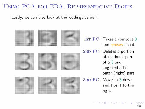
Using PCA for EDA: Representative Digits
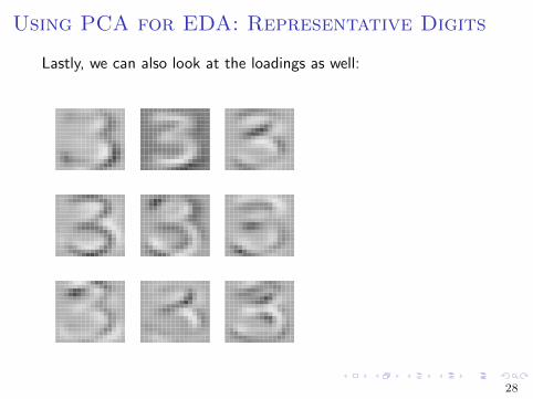
Lastly, we can also look at the loadings as well:
1st PC: Takes a compact 3and smears it out
2nd PC: Deletes a portionof the inner partof a 3 andaugments theouter (right) part
3rd PC: Moves a 3 downand tips it to theright
28
Using PCA for EDA: Representative Digits
Lastly, we can also look at the loadings as well:
1st PC: Takes a compact 3and smears it out
2nd PC: Deletes a portionof the inner partof a 3 andaugments theouter (right) part
3rd PC: Moves a 3 downand tips it to theright
28

Using PCA for EDA: Looking deeper
2.51∗ +0.63∗ +2.02∗
0.16∗ −4.55∗ +1.96∗=
> round(scores[1,1:6],2)
PC1 PC2 PC3 PC4 PC5 PC6
2.52 0.64 2.02 0.17 -4.55 1.9729

Decomposing in pixel axis versus PCA axis
Using 9 axis dimensions
30

Decomposing in pixel axis versus PCA axis
Using 100 axis dimensions
31
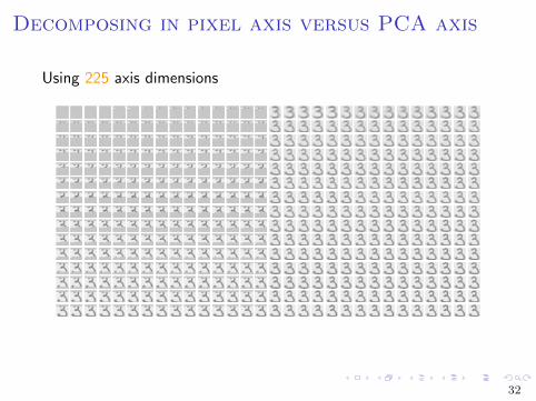
Decomposing in pixel axis versus PCA axis
Using 225 axis dimensions
32
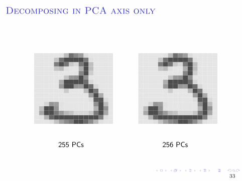
Decomposing in PCA axis only
255 PCs 256 PCs
33

Decomposing in pixel axis versus PCA axisWhat is this mystery figure?
This is the mean (From centering X : (X− X) = UDV>)(that is, the origin of the PCA axis, or X)1
plot.digit(attributes(digitsCenter)$’scaled:center’)
1Technically, X i for any i
34

Decomposing in pixel axis versus PCA axisWhat is this mystery figure?
This is the mean (From centering X : (X− X) = UDV>)(that is, the origin of the PCA axis, or X)1
plot.digit(attributes(digitsCenter)$’scaled:center’)
1Technically, X i for any i34

Two Common Uses of PCA
• Exploratory Data Analysis (EDA): Using the nature of theestimated rotation of our predictors to draw conclusions abouthow the predictors are related to each other.
• Principal Components Regression (PCR): Use the principalcomponents as the inputs to a regression procedure.
35
Principal Components Regression (PCR)
We can take PCA a bit further and use it in a more supervisedcapacity. Here’s the idea:
The PCs become the new predictors.(That is, the matrix UD in X−X = UDV>, or the x object returned by prcomp)
We don’t want to use all the PCs, however (this would beequivalent to using the original data). We have two choices:
• Use the scree plot to only include important PCs (those thatexplain the most variance).
• Use all the PCs, but do model selection.
We’ll concentrate on just doing the model selection approach(more justified theoretically).
36

Principal Components Regression (PCR)
It might seem strange to use the PCs (which are computedirrespective of the response Y ) as inputs to a regression.
Specifically, PCA estimates a feature of the marginal distributionof X (namely, its covariance)
Regression is interested in estimating the conditional distributionof Y |X (namely, the conditional mean of Y given X ).
37

Principal Components Regression (PCR)
This can be summarized in a quote by Mosteller and Tukey (1977)
... how can we find linear combinations of the [predictors] thatwill be likely, or unlikely, to pick up regression from some asyet specified Y ?
However, they responded to themselves in the same paper that
... A malicous person who knew our X ′s and our plan for themcould always invent a Y to make our choices look horrible. Butwe don’t believe that nature works that way – more nearly thatnature is, as Einstein put it, “tricky, but not downright mean.”
38

Principal Components Regression (PCR) in R
We can use someone’s function:
install.packages(’pls’)
library(pls)
pcr.fit = pcr(Y~., data=X,scale=TRUE,validation="CV")
This models our response versus the PC scores of the data X . Itchooses the number of PCs via CV.
39

Principal Components Regression (PCR):Example
We have data from 1986 showing 322 major league baseballplayers versus 20 variables:
AtBat: Number of times at bat in 1986
Hits: Number of hits in 1986
HmRun: Number of home runs in 1986
Runs: Number of runs in 1986
RBI: Number of runs batted in in 1986
Walks: Number of walks in 1986
Years: Number of years in the major leagues
CAtBat: Number of times at bat during his career
CHits: Number of hits during his career
CHmRun: Number of home runs during his career
CRuns: Number of runs during his career
CRBI: Number of runs batted in during his career
CWalks: Number of walks during his career
40

PCR Example: MLB Salary
(Continued)
League: A factor with levels A and N indicating league
at the end of 1986
Division: A factor with levels E and W
player’s division at the end of 1986
PutOuts: Number of put outs in 1986
Assists: Number of assists in 1986
Errors: Number of errors in 1986
NewLeague: A factor with levels A and N indicating
player’s league at the beginning of 1987
We would like to predict
Salary: 1987 annual salary on opening day in thousands
of dollars
41

PCR Example: MLB Salary
load(’../data/hitters.rda’)
> names(Hitters)
[1] "AtBat" "Hits" "HmRun" "Runs" "RBI"
[6] "Walks" "Years" "CAtBat" "CHits" "CHmRun"
[11] "CRuns" "CRBI" "CWalks" "League" "Division"
[16] "PutOuts" "Assists" "Errors" "Salary" "NewLeague"
> dim(Hitters)
[1] 322 20
> sum(is.na(Hitters$Salary))
[1] 59
> Hitters = na.omit(Hitters)
> dim(Hitters)
[1] 263 20
42

PCR Example: MLB Salary
The syntax for pcr is very similar to lm but with a few morearguments:
library(pls)
pcr.fit = pcr(Salary~., data=Hitters,scale=T,validation=’CV’)
A comment:
Question: What is random in this expression?
Answer: The CV part (randomly allocate data to validationsets).
43

PCR Example: MLB Salary
The syntax for pcr is very similar to lm but with a few morearguments:
library(pls)
pcr.fit = pcr(Salary~., data=Hitters,scale=T,validation=’CV’)
A comment:
Question: What is random in this expression?
Answer: The CV part (randomly allocate data to validationsets).
43

PCR Example: MLB Salary
Here is the output:
> summary(pcr.fit)
Data: X dimension: 263 19
Y dimension: 263 1
Fit method: svdpc
Number of components considered: 19
VALIDATION: RMSEP
Cross-validated using 10 random segments.
(Intercept) 1 comps 2 comps 3 comps 4 comps
CV 452 348.9 352.2 353.5 352.8
adjCV 452 348.7 351.8 352.9 352.1
....
18 comps 19 comps
CV 349.2 352.6
adjCV 346.7 349.8
44

PCR Example: MLB SalaryAdditionally, we can plot:
validationplot(pcr.fit,val.type="MSEP")
0 5 10 15
1200
0014
0000
1600
0018
0000
2000
00
Salary
number of components
MS
EP
45

PCR Example: MLB Salary
Let’s see how well it predicts. We will form a train and test split
train = sample(c(TRUE,FALSE), nrow(Hitters),rep=TRUE)
test = (!train)
And do a prediction:
pcr.fit = pcr(Salary~., data=Hitters,scale=T,
subset=train,validation=’CV’)
out.pcr = RMSEP(pcr.fit)
dim(out.pcr$val)
[1] 2 1 20
#Here
> out.pcr$comps[which.min(out.pcr$val[1,1,])]
[1] 5
46

PCR Example: MLB Salary
0 5 10 15
1000
0012
0000
1400
0016
0000
Salary
number of components
MS
EP
47

PCR Example: MLB Salary
pcr.fit = pcr(Salary~., data=Hitters,scale=T,subset=train,
validation=’CV’)
x = model.matrix(~.,data=Hitters)
y = Hitters$Salary
pcr.pred = predict(pcr.fit,x[test,-1],ncomp=5)
> sqrt(mean((pcr.pred - y[test])^2))
[1] 381.861
48

PCR Example: MLB Salary
Compare to, say, ridge regression
ridge.fit = cv.glmnet(x=x[train,],y=y[train],alpha=0)
ridge.pred = predict(ridge.fit,s=’lambda.min’,newx=x[test,])
> sqrt(mean((ridge.pred - y[test])^2))
[1] 388.674
So, we get a reduction of about 2% for PCR over ridge
Remember: PCR and ridge do not do any variable selection.They attempt to minimize prediction error by reducing variance
49
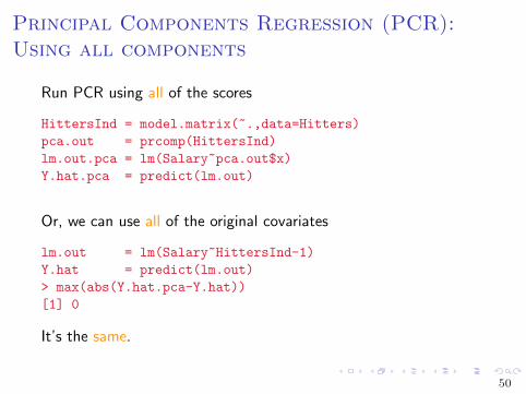
Principal Components Regression (PCR):Using all components
Run PCR using all of the scores
HittersInd = model.matrix(~.,data=Hitters)
pca.out = prcomp(HittersInd)
lm.out.pca = lm(Salary~pca.out$x)
Y.hat.pca = predict(lm.out)
Or, we can use all of the original covariates
lm.out = lm(Salary~HittersInd-1)
Y.hat = predict(lm.out)
> max(abs(Y.hat.pca-Y.hat))
[1] 0
It’s the same.
50