Des senseurs atomiques pour des tests de physique fondamentale en laboratoire et

dans l'espace

Peter Wolf LNE-SYRTE , Observatoire de Paris

Séminaire GReCO, Octobre 2007

CONTENTSCONTENTSCONTENTS

• The LNE-SYRTE clock ensemble• Tests of Lorentz invariance using a cryogenic resonator and a Cs

fountain clock (summary)• Variation of fundamental constants• SAGAS

The People who make it possible:

• S.Bize, F.Chapelet, P.Laurent, M.Abgrall, Y.Sortais, H.Marion, S.Zhang, F.Alard, I.Maksimovic, L.Cacciapuoti, J.Grünert, C.Vian, F.Pereira dos Santos, P.Rosenbusch, N.Dimarcq, P.Lemonde, G.Santarelli, A.Clairon, A.Luiten, M.Tobar, C.Salomon

• SAGAS collaboration (> 70 scientists)

+ ….

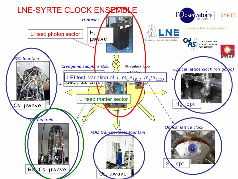
LNE-SYRTE CLOCK ENSEMBLE

Hg, opt

Sr, opt

Cs, µwave

Cs, µwave

Rb, Cs, µwave

H, µwave

Phaselock loop

τ~1000 s

FO1 fountain

FO2 fountain

FOM transportable fountainOptical lattice clock

Optical lattice clock (on going)

Macroscopicosc., 12 GHz

Cryogenic sapphire Osc.

H-maser

LI test: photon sector

LPI test: variation of α, mq/ΛQCD, me/ΛQCD

LI test: matter sector

Invariance de Lorentz (résumé)

• Invariance de Lorentz (LI): invariance de la physique dans un repère localement inertiel) sous changements d’orientation ou de vitesse.

• Postulat fondamental de la relativité ⇒ pilier de la physique moderne.• Théories de unification (théorie des cordes, gravitation quantique en

boucles, ….) admettent une violation de LI.⇒ forte motivations pour des tests de LI.

• Michelson-Morley, Kennedy-Thorndike, Ives-Stilwell, Hughes-Drever,….• Chercher une modification de la fréquence d’une cavité en fonction de la

direction de propagation de la lumière (orientation des champs E et B)• Chercher une modification de la fréquence d’une transition atomique en

fonction de l’orientation du spin.• Un cadre théorique très large pour décrire tous les tests de LI a été

développé récemment (Kostelecky et al.), l’extension du modèle standard (SME).

• Les travaux du SYRTE (en collaboration avec UWA) fournissent lesmeilleurs limites actuelles sur 16 paramètres du SME dans le secteur des photons et des protons. .

Variation of Fundamental ConstantsVariation Variation ofof FundamentalFundamental ConstantsConstants

Sébastien Bize, et al., J. Phys. B: At. Mol. Opt. Phys. 38 (2005) S449–S468

• Atomic transition frequencies and their dependence on fundamental constants

• Which constants vary? • How do they vary?• Recent results from clocks• Two positive results from astrophysics• Discussion and conclusion

.

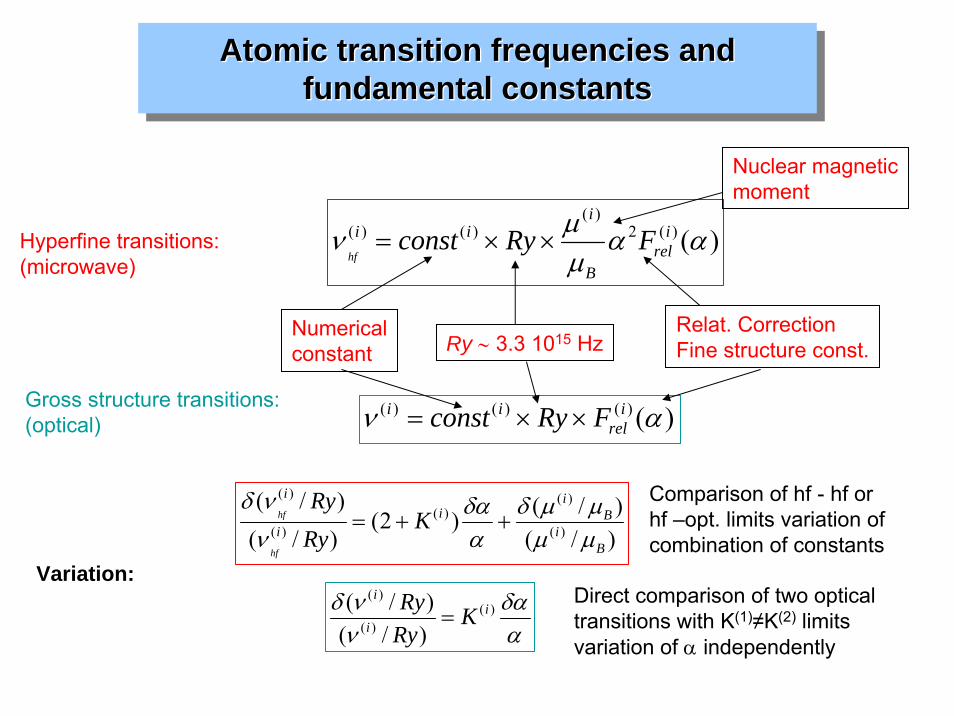
Atomic transition frequencies andfundamental constants

AtomicAtomic transition transition frequenciesfrequencies andandfundamentalfundamental constantsconstants

)()(2)(

)()( ααμμν i

relB

iii FRyconst

hf××=Hyperfine transitions:

(microwave)

Numericalconstant Ry ∼ 3.3 1015 Hz

Nuclear magneticmoment

Relat. CorrectionFine structure const.

Gross structure transitions:(optical) )()()()( αν i

relii FRyconst ××=

Variation:)/()/()2(

)/()/(

)(

)()(

)(

)(

Bi

Bi

ii

i

KRyRy

hf

hf

μμμμδ

αδα

ννδ

++=

αδα

ννδ )(

)(

)(

)/()/( i

i

i

KRyRy

=Direct comparison of two opticaltransitions with K(1)≠K(2) limitsvariation of α independently

Comparison of hf - hf orhf –opt. limits variation ofcombination of constants

Which constants vary?WhichWhich constants constants varyvary??

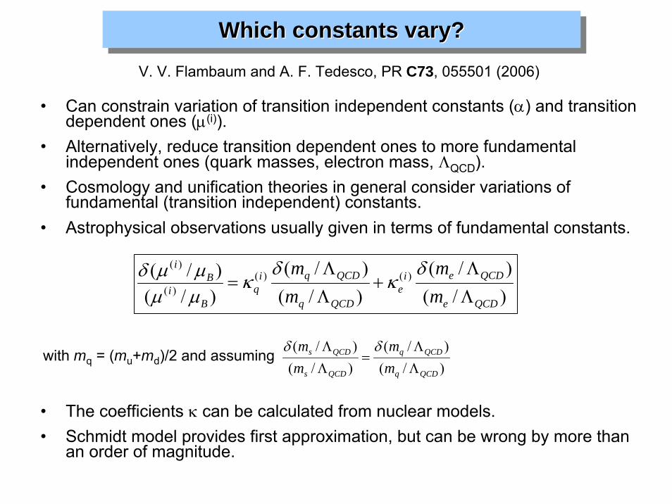
• Can constrain variation of transition independent constants (α) and transition dependent ones (μ(i)).

• Alternatively, reduce transition dependent ones to more fundamental independent ones (quark masses, electron mass, ΛQCD).

• Cosmology and unification theories in general consider variations of fundamental (transition independent) constants.

• Astrophysical observations usually given in terms of fundamental constants.

V. V. Flambaum and A. F. Tedesco, PR C73, 055501 (2006)

)/()/(

)/()/(

)/()/( )()(

)(

)(

QCDe

QCDeie

QCDq

QCDqiq

Bi

Bi

mm

mm

ΛΛ

+ΛΛ

=δ

κδ

κμμμμδ

with mq = (mu+md)/2 and assuming

• The coefficients κ can be calculated from nuclear models. • Schmidt model provides first approximation, but can be wrong by more than

an order of magnitude.

)/()/(

)/()/(

QCDq

QCDq

QCDs

QCDs

mm

mm

ΛΛ

=ΛΛ δδ

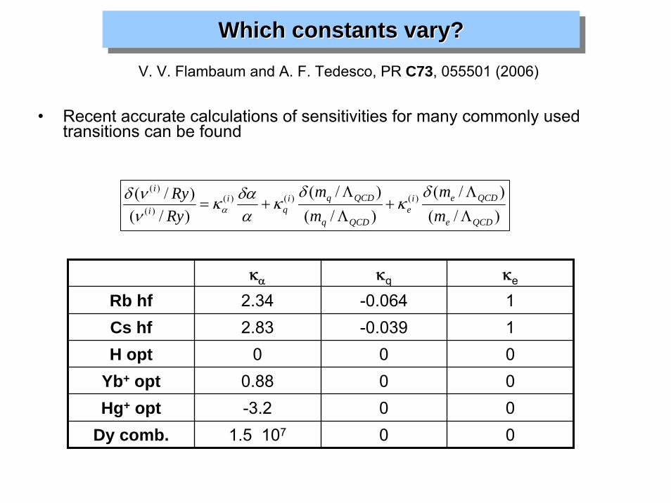
Which constants vary?WhichWhich constants constants varyvary??V. V. Flambaum and A. F. Tedesco, PR C73, 055501 (2006)

• Recent accurate calculations of sensitivities for many commonly used transitions can be found

)/()/(

)/()/(

)/()/( )()()(

)(

)(

QCDe

QCDeie

QCDq

QCDqiq

ii

i

mm

mm

RyRy

ΛΛ

+ΛΛ

+=δ

κδ

καδακ

ννδ

α

κα κq κe

Dy comb. 1.5 107 0 0

Rb hf 2.34 -0.064 1Cs hf 2.83 -0.039 1H opt 0 0 0

Yb+ opt 0.88 0 0Hg+ opt -3.2 0 0

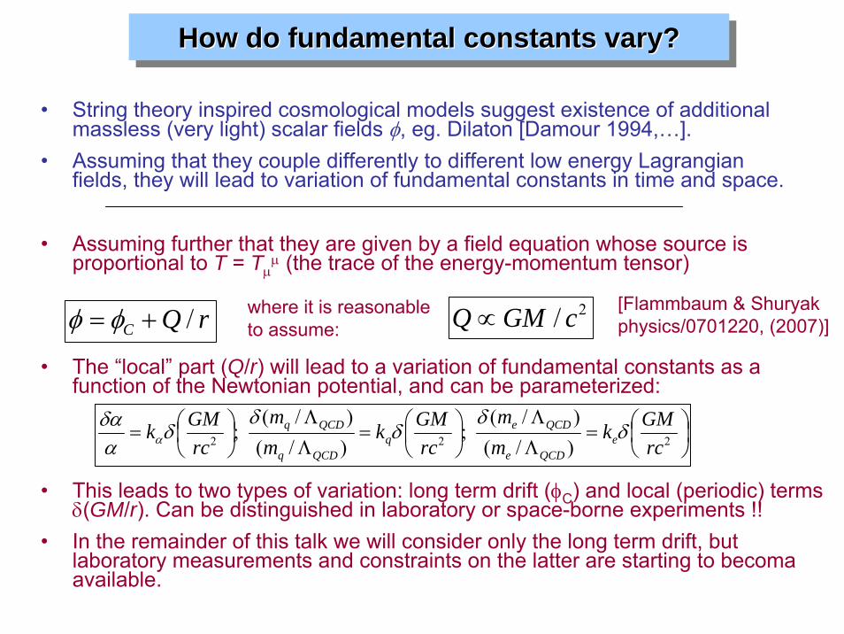
How do fundamental constants vary?HowHow do do fundamentalfundamental constants constants varyvary??

• String theory inspired cosmological models suggest existence of additional massless (very light) scalar fields φ, eg. Dilaton [Damour 1994,…].

• Assuming that they couple differently to different low energy Lagrangianfields, they will lead to variation of fundamental constants in time and space.

• Assuming further that they are given by a field equation whose source is proportional to T = Tμ

μ (the trace of the energy-momentum tensor)

⎟⎠⎞

⎜⎝⎛=

ΛΛ

⎟⎠⎞

⎜⎝⎛=

ΛΛ

⎟⎠⎞

⎜⎝⎛= 222 )/(

)/(;

)/()/(

;rcGMk

mm

rcGMk

mm

rcGMk e

QCDe

QCDeq

QCDq

QCDq δδ

δδ

δαδα

α

rQC /+= φφ where it is reasonableto assume:

2/ cGMQ ∝[Flammbaum & Shuryakphysics/0701220, (2007)]

• The “local” part (Q/r) will lead to a variation of fundamental constants as a function of the Newtonian potential, and can be parameterized:

• This leads to two types of variation: long term drift (φC) and local (periodic) terms δ(GM/r). Can be distinguished in laboratory or space-borne experiments !!

• In the remainder of this talk we will consider only the long term drift, but laboratory measurements and constraints on the latter are starting to becomaavailable.

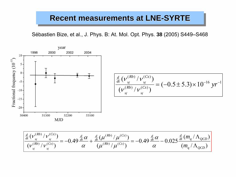
Recent measurements at LNE-SYRTERecentRecent measurementsmeasurements atat LNELNE--SYRTESYRTE

Sébastien Bize, et al., J. Phys. B: At. Mol. Opt. Phys. 38 (2005) S449–S468

116)()(

)()(

10)3.55.0()/()/(

−−×±−= yrCsRb

CsRbdtd

hfhf

hfhf

νννν

)/()/(

025.049.0)/()/(49.0

)/()/(

)()(

)()(

)()(

)()(

QCDq

QCDqdtd

dtd

CsRb

CsRbdtd

dtd

CsRb

CsRbdtd

mm

hfhf

hfhf

ΛΛ

−−=+−=αα

μμμμ

αα

νννν

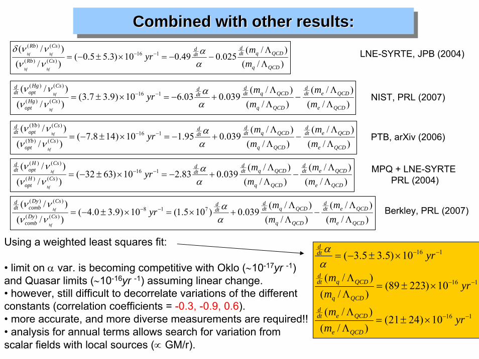
Combined with other results:CombinedCombined withwith otherother resultsresults::

)/()/(

)/()/(

039.003.610)9.37.3()/()/(

116)()(

)()(

QCDe

QCDedtd

QCDq

QCDqdtd

dtd

CsHgopt

CsHgoptdt

d

mm

mm

yrhf

hf

ΛΛ

−ΛΛ

+−=×±= −−

αα

νννν

)/()/(

025.049.010)3.55.0()/()/(

116)()(

)()(

QCDq

QCDqdtd

dtd

CsRb

CsRb

mm

yrhfhf

hfhf

ΛΛ

−−=×±−= −−

αα

ννννδ

)/()/(

)/()/(

039.095.110)148.7()/()/(

116)()(

)()(

QCDe

QCDedtd

QCDq

QCDqdtd

dtd

CsYbopt

CsYboptdt

d

mm

mm

yrhf

hf

ΛΛ

−ΛΛ

+−=×±−= −−

αα

νννν

)/()/(

)/()/(

039.083.210)6332()/()/(

116)()(

)()(

QCDe

QCDedtd

QCDq

QCDqdtd

dtd

CsHopt

CsHoptdt

d

mm

mm

yrhf

hf

ΛΛ

−ΛΛ

+−=×±−= −−

αα

νννν

LNE-SYRTE, JPB (2004)

NIST, PRL (2007)

PTB, arXiv (2006)

MPQ + LNE-SYRTE PRL (2004)

Using a weighted least squares fit:

• limit on α var. is becoming competitive with Oklo (∼10-17yr -1) and Quasar limits (∼10-16yr -1) assuming linear change.• however, still difficult to decorrelate variations of the different constants (correlation coefficients = -0.3, -0.9, 0.6).• more accurate, and more diverse measurements are required!!• analysis for annual terms allows search for variation from scalar fields with local sources (∝ GM/r).

116

116

116

10)2421()/()/(

10)22389()/()/(

10)5.35.3(

−−

−−

−−

×±=ΛΛ

×±=ΛΛ

×±−=

yrmm

yrmm

yr

QCDe

QCDedtd

QCDq

QCDqdtd

dtd

αα

)/()/(

)/()/(

039.0)105.1(10)9.30.4()/()/(

718)()(

)()(

QCDe

QCDedtd

QCDq

QCDqdtd

dtd

CsDycomb

CsDycombdt

d

mm

mm

yrhf

hf

ΛΛ

−ΛΛ

+×=×±−= −−

αα

νννν

Berkley, PRL (2007)

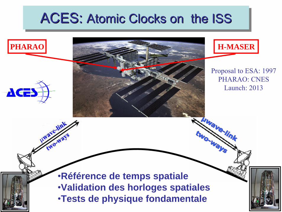
ACES: Atomic Clocks on the ISSACES: ACES: AtomicAtomic ClocksClocks on the ISSon the ISS

PHARAO H-MASER

Proposal to ESA: 1997PHARAO: CNES

Launch: 2013

•Référence de temps spatiale•Validation des horloges spatiales•Tests de physique fondamentale

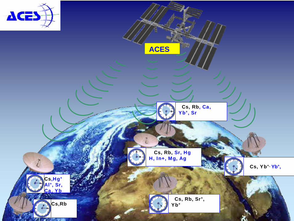
ACES

Cs, Rb, Ca, Yb+, Sr

Cs, Yb+, Yb+,

Cs, Rb, Sr, HgH, In+, Mg, Ag

Cs,Hg+

Al+, Sr,Ca, Yb

Cs, Rb, Sr+, Yb+Cs,Rb

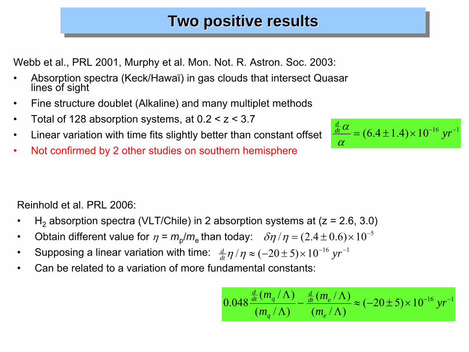
Two positive resultsTwoTwo positive positive resultsresults

Webb et al., PRL 2001, Murphy et al. Mon. Not. R. Astron. Soc. 2003:• Absorption spectra (Keck/Hawaï) in gas clouds that intersect Quasar

lines of sight• Fine structure doublet (Alkaline) and many multiplet methods• Total of 128 absorption systems, at 0.2 < z < 3.7• Linear variation with time fits slightly better than constant offset• Not confirmed by 2 other studies on southern hemisphere

11610)4.14.6( −−×±= yrdtd

αα

Reinhold et al. PRL 2006:• H2 absorption spectra (VLT/Chile) in 2 absorption systems at (z = 2.6, 3.0)• Obtain different value for η = mp/me than today: • Supposing a linear variation with time:• Can be related to a variation of more fundamental constants:

11610)520(/ −−×±−≈ yrdtd ηη

510)6.04.2(/ −×±=ηδη

11610)520()/()/(

)/()/(

048.0 −−×±−≈ΛΛ

−ΛΛ

yrmm

mm

e

edtd

q

qdtd

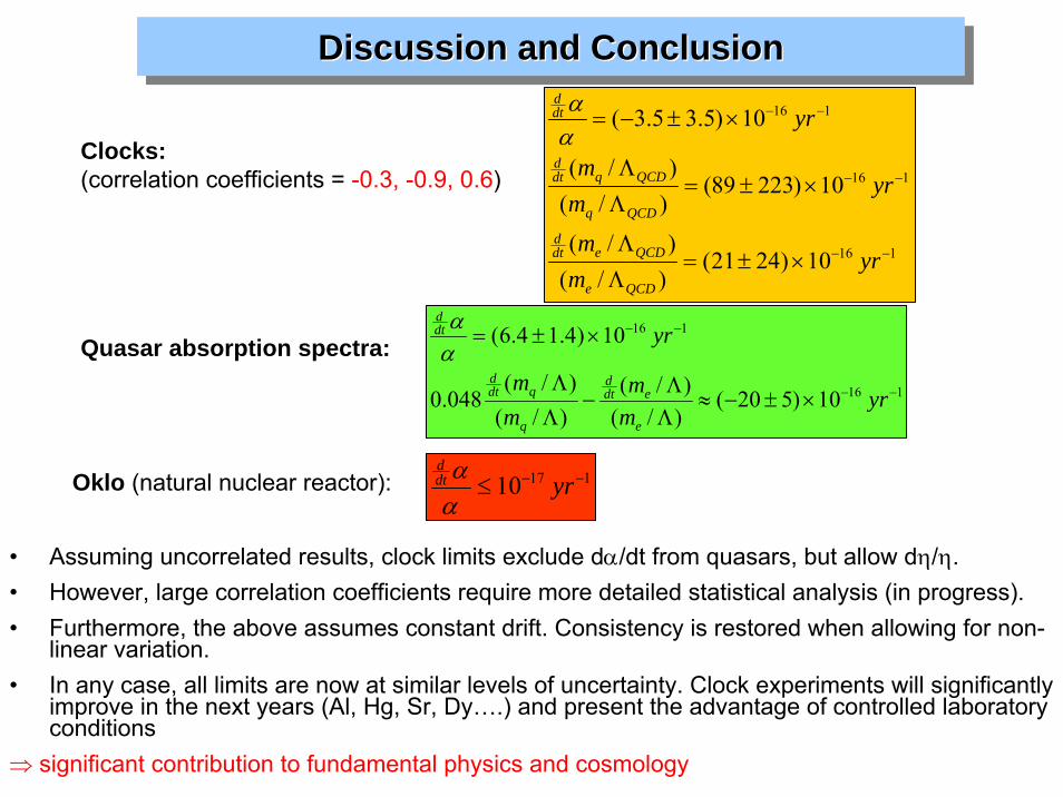
Discussion and ConclusionDiscussion Discussion andand ConclusionConclusion

11710 −−≤ yrdtd

ααOklo (natural nuclear reactor):

Clocks:(correlation coefficients = -0.3, -0.9, 0.6)

Quasar absorption spectra:116

116

10)520()/()/(

)/()/(

048.0

10)4.14.6(

−−

−−

×±−≈ΛΛ

−ΛΛ

×±=

yrmm

mm

yr

e

edtd

q

qdtd

dtd

αα

• Assuming uncorrelated results, clock limits exclude dα/dt from quasars, but allow dη/η.• However, large correlation coefficients require more detailed statistical analysis (in progress).• Furthermore, the above assumes constant drift. Consistency is restored when allowing for non-

linear variation.• In any case, all limits are now at similar levels of uncertainty. Clock experiments will significantly

improve in the next years (Al, Hg, Sr, Dy….) and present the advantage of controlled laboratory conditions

⇒ significant contribution to fundamental physics and cosmology

116

116

116

10)2421()/()/(

10)22389()/()/(

10)5.35.3(

−−

−−

−−

×±=ΛΛ

×±=ΛΛ

×±−=

yrmm

yrmm

yr

QCDe

QCDedtd

QCDq

QCDqdtd

dtd

αα

peter.wolf@obspm.fr

DES SENSEURS POUR EXPLORER LA GRAVITATION DANS LE SYSTÈME SOLAIRE

(Le projet SAGAS)

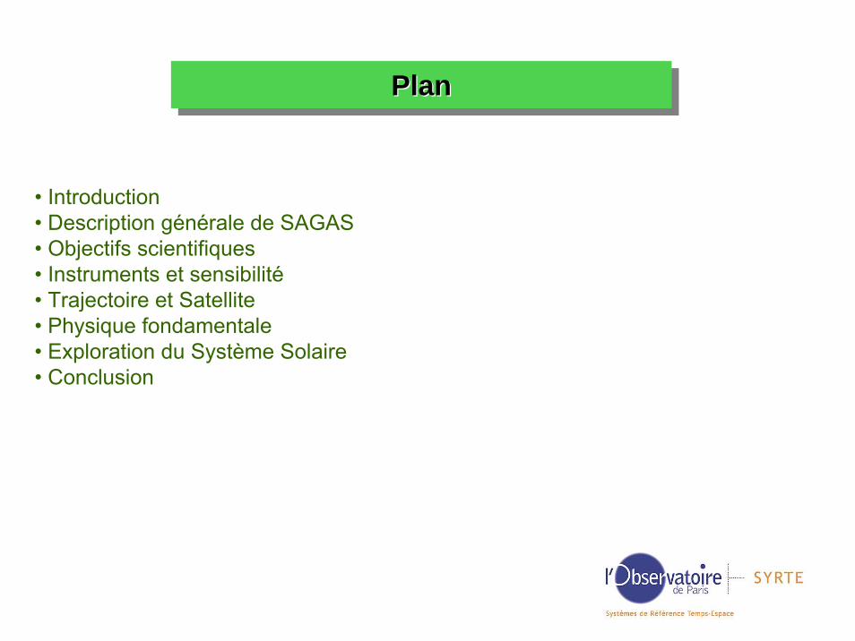
PlanPlanPlan

• Introduction• Description générale de SAGAS• Objectifs scientifiques• Instruments et sensibilité• Trajectoire et Satellite• Physique fondamentale• Exploration du Système Solaire• Conclusion

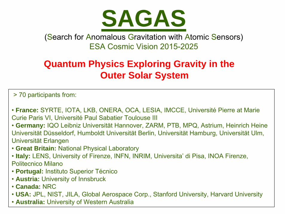
SAGAS(Search for Anomalous Gravitation with Atomic Sensors)

ESA Cosmic Vision 2015-2025

Quantum Physics Exploring Gravity in theOuter Solar System

> 70 participants from:

• France: SYRTE, IOTA, LKB, ONERA, OCA, LESIA, IMCCE, Université Pierre at Marie Curie Paris VI, Université Paul Sabatier Toulouse III• Germany: IQO Leibniz Universität Hannover, ZARM, PTB, MPQ, Astrium, Heinrich Heine Universität Düsseldorf, Humboldt Universität Berlin, Universität Hamburg, Universität Ulm, Universität Erlangen• Great Britain: National Physical Laboratory• Italy: LENS, University of Firenze, INFN, INRIM, Universita’ di Pisa, INOA Firenze, Politecnico Milano• Portugal: Instituto Superior Técnico• Austria: University of Innsbruck• Canada: NRC• USA: JPL, NIST, JILA, Global Aerospace Corp., Stanford University, Harvard University• Australia: University of Western Australia

IntroductionIntroductionIntroduction

• Gravitation is well described by General relativity (GR).• GR is a classical theory, which shows inconsistencies with quantum field theory.• All unification models predict (small) deviations of gravitation laws from GR.• Gravity is well explored at small (laboratory) to medium (Moon, inner planets) distance scales.• At very large distances (galxies, cosmology) some puzzles remain (galactic rotation curves, SNR redshifts, dark matter and energy, ….).• The largest distances explored by man-made artefacts are of the size of the outer solar system ⇒ carry out precision gravitational measurements in outer solar system.

• Kuiper Belt (≈ 40 AU, ≈ 1000 KBOs since 1992), the disk from which giant planets formed is largely unexplored.• Known mass (MKB ≈ 10-1 ME) about 100 times too small for in situ formation of KBOs.• KBO masses only inferred from albedo and density hypothesis (⇒ uncertainty).• “In situ” gravitational measurements yields exceptional information on MKB, overall mass distribution, and individual KBO masses (+ discover new KBOs ?)• Measurements during planetary fly by (Jupiter) can yield highly accurate determination of planetary gravity.

SAGAS: OverviewSAGAS: SAGAS: OverviewOverview

Payload:1. Cold atom absolute accelerometer, 3 axis measurement of local non-gravitational

acceleration.2. Optical atomic clock, absolute frequency measurement (local proper time).3. Laser link (frequency comparison + Doppler for navigation).

Trajectory:• Jupiter flyby and gravity assist (≈ 3 years after launch).• Reach distance of ≈39 AU (15 yrs nominal) to ≈53 AU (20 yrs, extended).

Measurements:• Gravitational trajectory of test body (S/C): using Doppler ranging and correcting for

non-gravitational forces using accelerometer measurements.• Gravitational frequency shift of local proper time: using clock and laser link to

ground clocks for frequency comparison.⇒ Measure all aspects of gravity !

Science Objectives: OverviewScience Objectives: Science Objectives: OverviewOverview

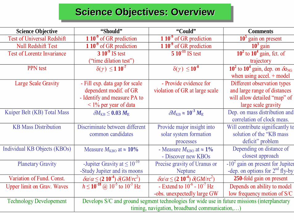
Science Objective “Should” “Could” Comments Test of Universal Redshift 1 10-9 of GR prediction 1 10-9 of GR prediction 105 gain on present

Null Redshift Test 1 10-9 of GR prediction 1 10-9 of GR prediction 103 gain Test of Lorentz Invariance 3 10-9 IS test

(“time dilation test”) 5 10-11 IS test 102 to 104 gain, fct. of

trajectory PPN test δ(γ ) ≤ 1 10-7 δ(γ ) ≤ 10-8 102 to 104 gain, dep. on δaNG

when using accel. + model Large Scale Gravity - Fill exp. data gap for scale

dependent modif. of GR - Identify and measure PA to

< 1% per year of data

- Provide evidence for violation of GR at large scale

Different observation types and large range of distances will allow detailed “map” of

large scale gravity Kuiper Belt (KB) Total Mass δMKB ≤ 0.03 ME δMKB ≈ 10-3 ME Dep. on mass distribution and

correlation of clock meas. KB Mass Distribution Discriminate between different

common candidates Provide major insight into

solar system formation processes

Will contribute significantly to solution of the “KB mass

deficit” problem Individual KB Objects (KBOs) Measure MKBO at ≈ 10% - Measure MKBO at ≈ 1%

- Discover new KBOs Depending on distance of

closest approach Planetary Gravity -Jupiter Gravity at ≤ 10-10

-Study Jupiter and its moons Precise gravity of Uranus or

Neptune -102 gain on present for Jupiter -dep. on options for 2nd fly-by

Variation of Fund. Const. δα/α ≤ (2 10-4) δ(GM/rc2) δα/α ≤ (2 10-4) δ(GM/rc2) 250-fold gain on present Upper limit on Grav. Waves h ≤ 10-18 @ 10-5 to 10-3 Hz - Extend to 10-6 - 10-7 Hz

-obs. unexpectedly large GW Depends on ability to model low frequency motion of S/C

Technology Developement Develops S/C and ground segment technologies for wide use in future missions (interplanetary timing, navigation, broadband communication,…)

Payload: AccelerometerPayloadPayload: : AccelerometerAccelerometer

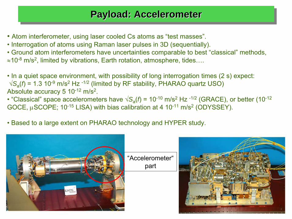
• Atom interferometer, using laser cooled Cs atoms as “test masses”.• Interrogation of atoms using Raman laser pulses in 3D (sequentially).• Ground atom interferometers have uncertainties comparable to best “classical” methods, ≈10-8 m/s2, limited by vibrations, Earth rotation, atmosphere, tides….

• In a quiet space environment, with possibility of long interrogation times (2 s) expect: √Sa(f) = 1.3 10-9 m/s2 Hz -1/2 (limited by RF stability, PHARAO quartz USO)Absolute accuracy 5 10-12 m/s2.• “Classical” space accelerometers have √Sa(f) = 10-10 m/s2 Hz -1/2 (GRACE), or better (10-12

GOCE, μSCOPE; 10-15 LISA) with bias calibration at 4 10-11 m/s2 (ODYSSEY).

• Based to a large extent on PHARAO technology and HYPER study.

“Accelerometer“part

Payload: Optical ClockPayloadPayload: : OpticalOptical ClockClock

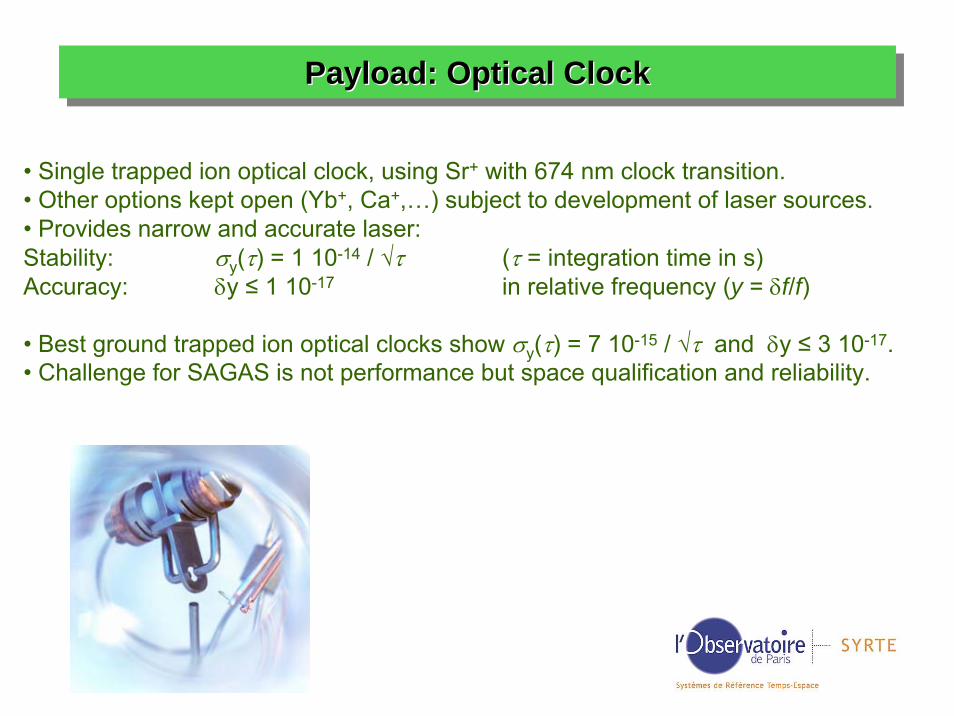
• Single trapped ion optical clock, using Sr+ with 674 nm clock transition.• Other options kept open (Yb+, Ca+,…) subject to development of laser sources.• Provides narrow and accurate laser: Stability: σy(τ) = 1 10-14 / √τ (τ = integration time in s)Accuracy: δy ≤ 1 10-17 in relative frequency (y = δf/f)

• Best ground trapped ion optical clocks show σy(τ) = 7 10-15 / √τ and δy ≤ 3 10-17.• Challenge for SAGAS is not performance but space qualification and reliability.

Payload: Optical LinkPayloadPayload: : OpticalOptical LinkLink

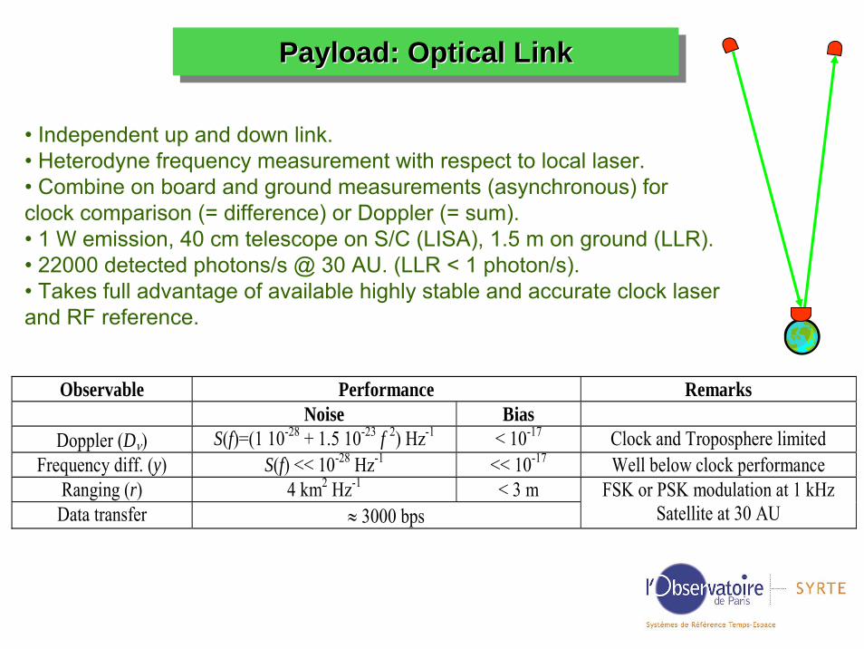
• Independent up and down link.• Heterodyne frequency measurement with respect to local laser.• Combine on board and ground measurements (asynchronous) for clock comparison (= difference) or Doppler (= sum).• 1 W emission, 40 cm telescope on S/C (LISA), 1.5 m on ground (LLR).• 22000 detected photons/s @ 30 AU. (LLR < 1 photon/s).• Takes full advantage of available highly stable and accurate clock laser and RF reference.

Observable Performance Remarks Noise Bias

Doppler (Dν) S(f)=(1 10-28 + 1.5 10-23 f 2) Hz-1 < 10-17 Clock and Troposphere limited Frequency diff. (y) S(f) << 10-28 Hz-1 << 10-17 Well below clock performance

Ranging (r) 4 km2 Hz-1 < 3 m Data transfer ≈ 3000 bps

FSK or PSK modulation at 1 kHz Satellite at 30 AU

Trajectory and SpacecraftTrajectoryTrajectory andand SpacecraftSpacecraft

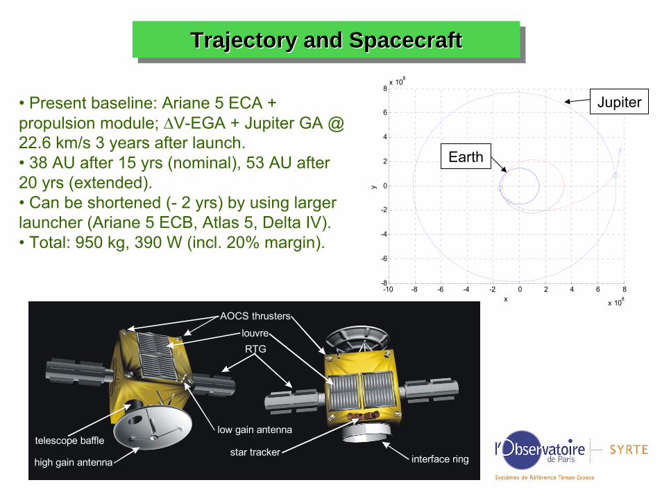
• Present baseline: Ariane 5 ECA + propulsion module; ΔV-EGA + Jupiter GA @ 22.6 km/s 3 years after launch.• 38 AU after 15 yrs (nominal), 53 AU after 20 yrs (extended).• Can be shortened (- 2 yrs) by using larger launcher (Ariane 5 ECB, Atlas 5, Delta IV).• Total: 950 kg, 390 W (incl. 20% margin).

-10 -8 -6 -4 -2 0 2 4 6 8

x 108

-8

-6

-4

-2

0

2

4

6

8x 108

x

y

Earth

Jupiter

RTGlouvre

high gain antenna

low gain antenna

star trackerinterface ring

AOCS thrusters

telescope baffle

Fundamental Physics: Non-metric gravityFundamentalFundamental PhysicsPhysics: : NonNon--metricmetric gravitygravity

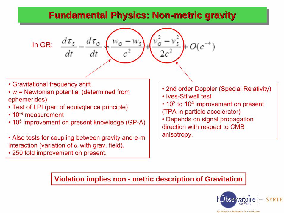
In GR:

• Gravitational frequency shift• w = Newtonian potential (determined fromephemerides)• Test of LPI (part of equivqlence principle)• 10-9 measurement• 105 improvement on present knowledge (GP-A)

• Also tests for coupling between gravity and e-m interaction (variation of α with grav. field).• 250 fold improvement on present.

• 2nd order Doppler (Special Relativity)• Ives-Stilwell test• 102 to 104 improvement on present(TPA in particle accelerator)• Depends on signal propagationdirection with respect to CMB anisotropy.

Violation implies non - metric description of Gravitation

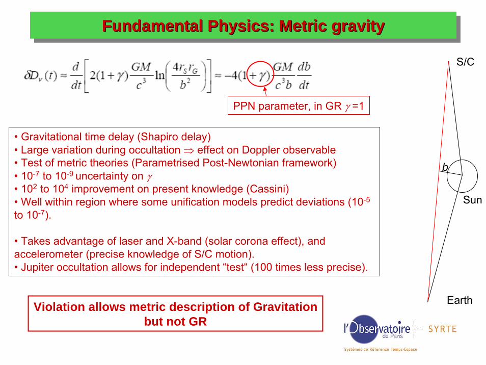
Fundamental Physics: Metric gravityFundamentalFundamental PhysicsPhysics: : MetricMetric gravitygravity

• Gravitational time delay (Shapiro delay) • Large variation during occultation ⇒ effect on Doppler observable• Test of metric theories (Parametrised Post-Newtonian framework)• 10-7 to 10-9 uncertainty on γ• 102 to 104 improvement on present knowledge (Cassini)• Well within region where some unification models predict deviations (10-5

to 10-7).

• Takes advantage of laser and X-band (solar corona effect), and accelerometer (precise knowledge of S/C motion).• Jupiter occultation allows for independent “test“ (100 times less precise).

Sun

S/C

Earth

b

PPN parameter, in GR γ =1

Violation allows metric description of Gravitationbut not GR

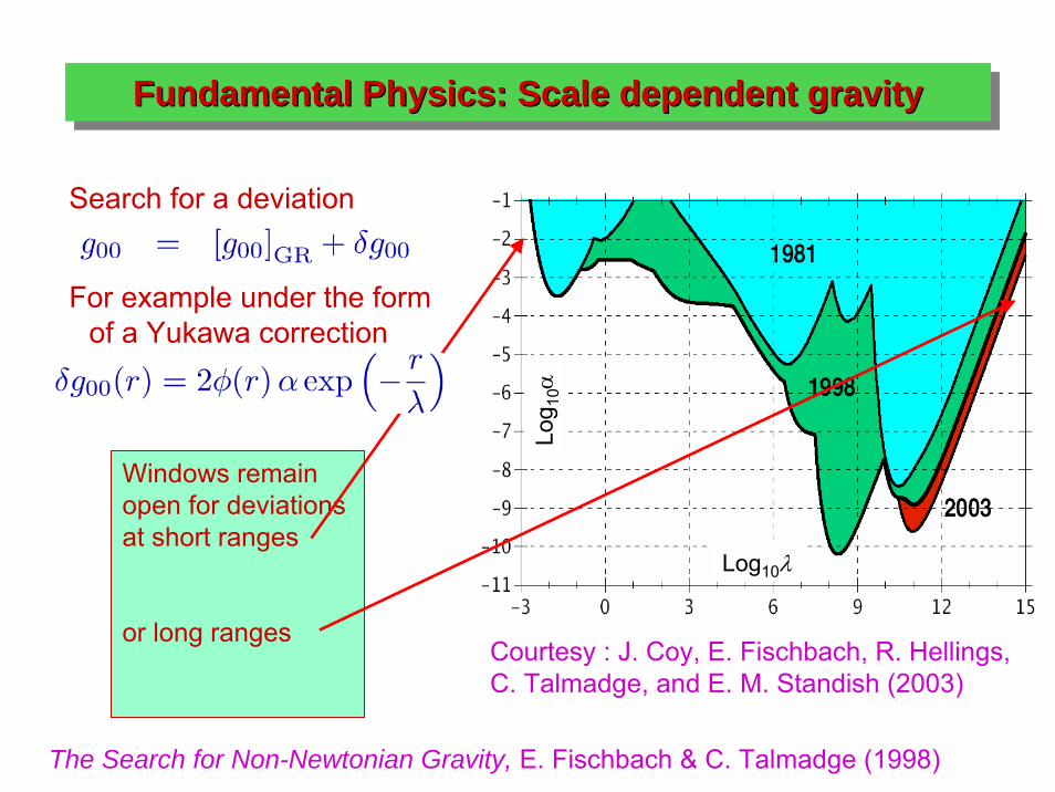
Courtesy : J. Coy, E. Fischbach, R. Hellings, C. Talmadge, and E. M. Standish (2003)

Windows remain open for deviations at short ranges

or long ranges

The Search for Non-Newtonian Gravity, E. Fischbach & C. Talmadge (1998)

Search for a deviation

For example under the form of a Yukawa correction

Fundamental Physics: Scale dependent gravityFundamentalFundamental PhysicsPhysics: : ScaleScale dependentdependent gravitygravity

Log 1

0αLog10λ

Fundamental Physics:Large scale gravity test (Pioneer example)

Fundamental Physics:Fundamental Physics:Large scale gravity test (Pioneer example)Large scale gravity test (Pioneer example)

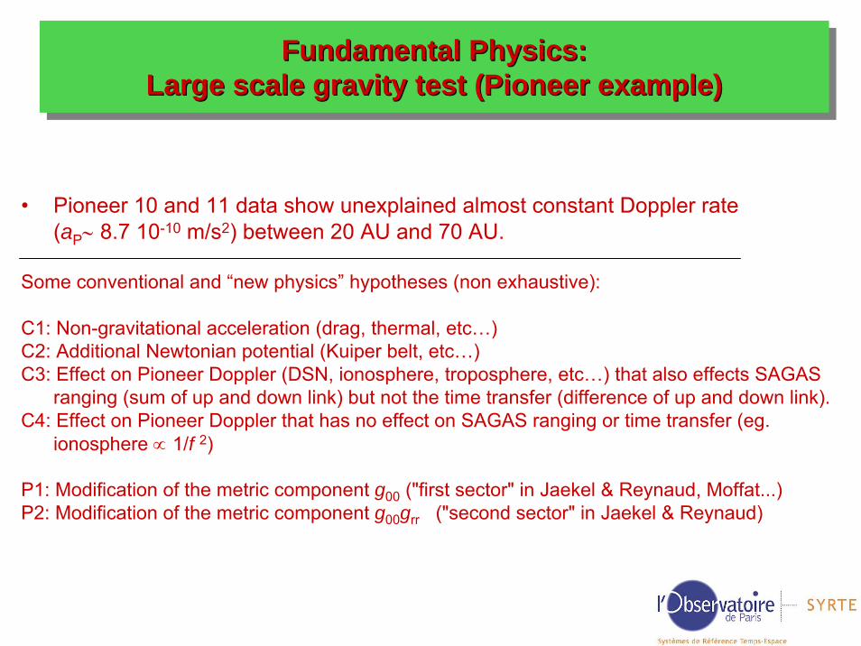
• Pioneer 10 and 11 data show unexplained almost constant Doppler rate (aP∼ 8.7 10-10 m/s2) between 20 AU and 70 AU.

Some conventional and “new physics” hypotheses (non exhaustive):

C1: Non-gravitational acceleration (drag, thermal, etc…)C2: Additional Newtonian potential (Kuiper belt, etc…)C3: Effect on Pioneer Doppler (DSN, ionosphere, troposphere, etc…) that also effects SAGAS

ranging (sum of up and down link) but not the time transfer (difference of up and down link).C4: Effect on Pioneer Doppler that has no effect on SAGAS ranging or time transfer (eg.

ionosphere ∝ 1/f 2)

P1: Modification of the metric component g00 ("first sector" in Jaekel & Reynaud, Moffat...)P2: Modification of the metric component g00grr ("second sector" in Jaekel & Reynaud)

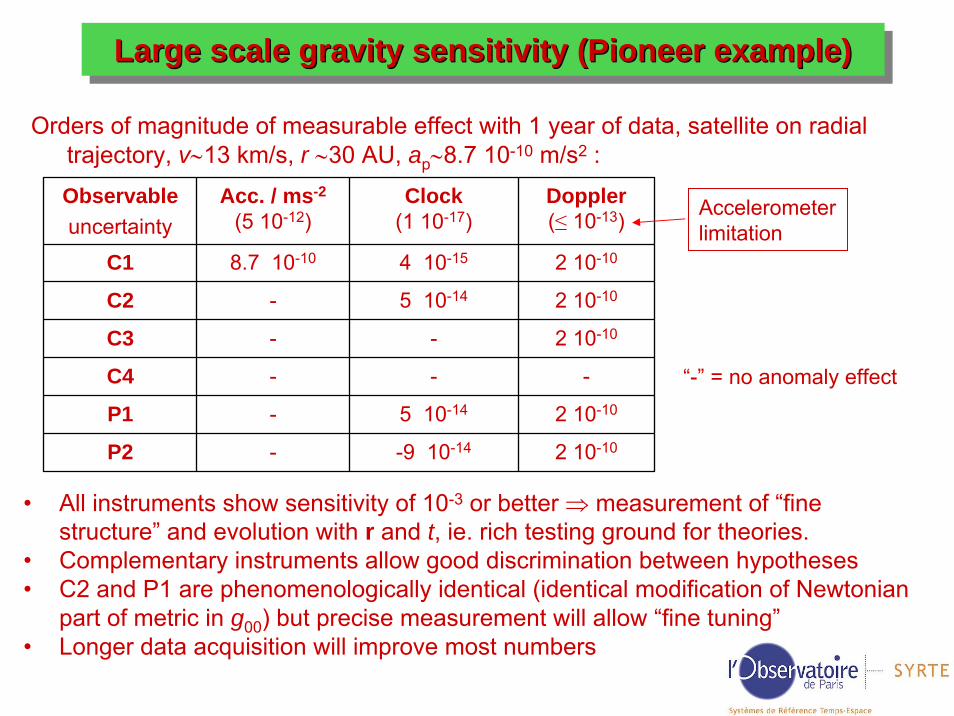
Large scale gravity sensitivity (Pioneer example)Large scale gravity sensitivity (Pioneer example)Large scale gravity sensitivity (Pioneer example)

Orders of magnitude of measurable effect with 1 year of data, satellite on radial trajectory, v∼13 km/s, r ∼30 AU, ap∼8.7 10-10 m/s2 :

Observableuncertainty

Acc. / ms-2

(5 10-12)Clock

(1 10-17)Doppler(≤ 10-13)

C1 8.7 10-10 4 10-15 2 10-10

C2 - 5 10-14 2 10-10

C3 - - 2 10-10

C4 - - -

P1 - 5 10-14 2 10-10

P2 - -9 10-14 2 10-10

• All instruments show sensitivity of 10-3 or better ⇒ measurement of “fine structure” and evolution with r and t, ie. rich testing ground for theories.

• Complementary instruments allow good discrimination between hypotheses• C2 and P1 are phenomenologically identical (identical modification of Newtonian

part of metric in g00) but precise measurement will allow “fine tuning”• Longer data acquisition will improve most numbers

“-” = no anomaly effect

Accelerometer limitation

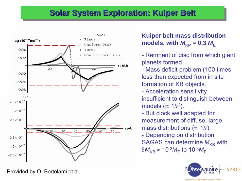
Kuiper belt mass distribution models, with MKP = 0.3 ME

- Remnant of disc from which giant planets formed.- Mass deficit problem (100 times less than expected from in situ formation of KB objects.- Acceleration sensitivity insufficient to distinguish between models (∝ 1/r2).- But clock well adapted for measurement of diffuse, large mass distributions (∝ 1/r).- Depending on distribution SAGAS can determine MKB with δMKB ≈ 10-2ME to 10-3ME

Provided by O. Bertolami et al.

Solar System Exploration: Kuiper BeltSolar System Exploration: Solar System Exploration: KuiperKuiper BeltBelt

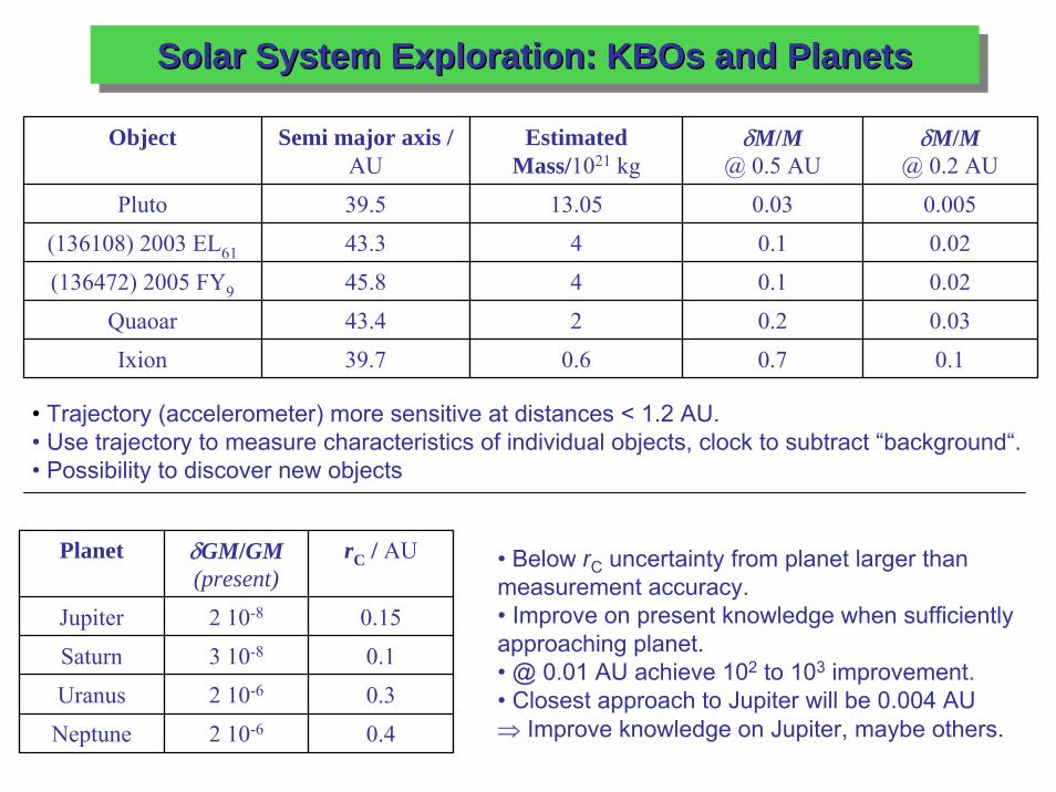
Solar System Exploration: KBOs and PlanetsSolar System Exploration: Solar System Exploration: KBOsKBOs and Planetsand Planets

Object Semi major axis / AU

Estimated Mass/1021 kg

δM/M@ 0.5 AU

δM/M@ 0.2 AU

Pluto 39.5 13.05 0.03 0.005

(136108) 2003 EL61 43.3 4 0.1 0.02

(136472) 2005 FY9 45.8 4 0.1 0.02

Quaoar 43.4 2 0.2 0.03

Ixion 39.7 0.6 0.7 0.1

Planet δGM/GM(present)

rC / AU

Jupiter 2 10-8 0.15

Saturn 3 10-8 0.1

Uranus 2 10-6 0.3

Neptune 2 10-6 0.4

• Trajectory (accelerometer) more sensitive at distances < 1.2 AU.• Use trajectory to measure characteristics of individual objects, clock to subtract “background“.• Possibility to discover new objects

• Below rC uncertainty from planet larger thanmeasurement accuracy.• Improve on present knowledge when sufficientlyapproaching planet.• @ 0.01 AU achieve 102 to 103 improvement.• Closest approach to Jupiter will be 0.004 AU⇒ Improve knowledge on Jupiter, maybe others.

Astronomy and Cosmology:Upper limits on low frequency grav. Waves (GW)

Astronomy and Cosmology:Astronomy and Cosmology:Upper limits on low frequency Upper limits on low frequency gravgrav. Waves (GW). Waves (GW)

• Doppler observable can be used to search for GW of frequency ≈ c/L.• Strain sensitivity ≈ 10-14/√Hz at 10-5 to 10-3 Hz.

• Insufficient to constrain cosmic stochastic GW background below presentlimits (Pulsar timing).• Would need to extend to 10-7 to 10-6 Hz (model for non-grav. accelerations?).

• For particular sources in the 10-5 to 10-3 Hz region can use template and optimal filtering. With one year data achieve h ≤ 10-18.• Insufficient for expected sources (eg. for BHB expect h ≤ 10-19).• But may be usefull for constraints on astrophysical models, and leaves dooropen for surprises.

ConclusionConclusionConclusion

SAGAS offers a unique possibility for a mission combining equally attractive objectives in fundamental physics and solar system exploration.

• Allows testing gravity at distance scales and with a sensitivity unattainable in ground or terrestrial orbit experiments.• Theory (unification models) expects to see modifications of known physics, in particular of GR, in sensitivity regions probed by SAGAS.• Observation at very large scales (galaxies, cosmology) also gives rise to some interrogation ⇒ design controlled experiments at largest possible distances.• Potential for a major discovery in physics and major contribution to constraining theoretical models.• Kuiper Belt (KB) potentially holds clues for planetary formation processes, and gives rise to fundamental questions (mass deficit?).• KB objects (KBOs) very distant, small, and difficult to observe⇒ in situ gravitational measurements provide valuable information on KB total mass, KB mass distribution, and individual KBOs.• Planetary fly by (Jupiter in particular) will allow significant improvement on knowledge of its gravity and thus the planetary system as a whole.• Major contribution to the understanding of planetary formation in the solar system, with potential for new discoveries (KB mass, new KBOs).