Embed Size (px)
DESCRIPTION
This paper gives the copper solvent extraction simulation method based on the realistic theory. This method is simply to use for any complex configuration of copper solvent extraction (series-parallel, interlaced, and others).
Citation preview
Joseph Kafumbila Process Designer
Design of Copper solvent extraction configurations
Copyright © 2015 Joseph Kafumbila [email protected]
www.linkedin.com
Joseph Kafumbila | Process designer-2015
2
Content Preface………………………………………………………………………………... 2 1. Modeling and Isotherm of copper solvent extraction………………………………….. 3 1.1. Extraction step…………………………………………………………………. 3 1.1.1. Modeling of extraction……………………………………………….. 3 1.1.2. Isotherm of extraction……………………………………………….. 7 1.1.3. Maximum copper concentration in the organic phase……………….. 11 1.2. Stripping step………………………………………………………………….. 12 1.2.1. Modeling of stripping………………………………………………… 12 1.2.2. Isotherm of stripping step……………………………………………. 14 1.2.3. Minimum copper concentration in the stripped organic……………… 16 2. Mass balance of copper solvent extraction……………………………………………. 17 2.1. Scheme of stage on the extraction and the stripping step………………………. 17 2.2. Flow parameters of copper solvent extraction…………………………………. 18 2.3. Equations of mass balance of copper solvent extraction……………………….. 18 2.3.1. Extraction step………………………………………………………. 18 2.3.2. Stripping step………………………………………………………… 20 2.3.3. Equilibrium constraints between the extraction and the stripping steps 22 2.4. Mixing efficiency……………………………………………………………….. 22 2.4.1. Description of mixing efficiency……………………………………… 22 2.4.2. Flow parameters……………………………………………………… 23 2.4.3. Correlations of concentrations of copper…………………………….. 23 2.4.4. Industrial data of mixing efficiency…………………………………… 24 2.5. MacCabe Thiele diagram……………………………………………………….. 24 2.5.1. Extraction step………………………………………………………. 24 2.5.2. Stripping step………………………………………………………… 25 3 Simulation of solvent extraction scheme………………………………………………. 26 3.1. Constraints of copper SX/EW configuration…………………………………... 26 3.1.1 Maximum value of V% in the organic phase…………………………. 26 3.1.2. PLS and spent electrolytes temperature………………………………. 26 3.1.3. Free acid concentration in the PLS…………………………………… 26 3.1.4. Maximum concentration of free acid in the spent electrolyte…………. 27 3.1.5. Minimum concentration of copper in the spent electrolyte…………… 27 3.1.6. Maximum concentration of copper in the advance electrolyte………... 28 3.1.7. Minimum value of
……………………………………………….. 28
3.1.8. Maximum value of ……………………………………………….. 29
3.2. Optimum value of volume percentage of extractant in the organic……………. 30 3.2.1. Constraints…………………………………………………………… 30 3.2.2. Maximum extraction efficiency……………………………………….. 31 3.2.3. Saturation of organic phase with the copper…………………………. 32 3.3. Procedure of copper solvent extraction simulation…………………………….. 34 3.3.1. Plant description…………………………………………………….. 34 3.3.2. Simulation procedure………………………………………………… 34 References……………………………………………………………………………. 50
Joseph Kafumbila | Process designer-2015
3
Preface
The aim of this paper is to present a simple method of simulation based on the realistic theory of copper solvent extraction and easy to use on an Excel spreadsheet for any complex scheme. This method is intended for designers of copper solvent extraction plants.
In the first chapter, this paper gives the equilibrium correlations on the extraction and the stripping step of copper solvent extraction using the extractant Lix984N. This extractant is chosen because it is the most used in the metallurgy of copper. The equilibrium correlation on the extraction step is based on the thermodynamic property of chemical reaction of copper solvent extraction. The equilibrium correlation on the stripping step is based on the characteristics of isotherm curves. In this chapter, the procedure of construction of isotherms curves is given for the extraction and stripping steps. The equilibrium correlation on the extraction step gives also the mathematical expression for the calculation of maximum load value.
In the second chapter, this paper gives the conservation equations of volume and mass in the copper solvent extraction plant, the values of parameters such as the extraction and the stripping efficiencies, the equilibrium constraints between the extraction and the stripping steps, the mathematical expressions of mixing efficiencies, and MacCabe Thiele diagram of extraction and stripping steps.
In the last chapter, it gives the limitations of values of design criteria and the simulation procedure of copper solvent extraction using the equilibrium correlations developed in the first chapter.
Joseph Kafumbila | Process designer-2015
4
1. Modeling and isotherm of copper solvent extraction 1.1. Extraction step 1.1.1. Modeling of extraction
The extraction stage depends on the kinetics of mass transfer between both phases (organic and aqueous) and the transfer is stopped when the copper is reached the thermodynamic equilibrium in both phases.
The Lix 984N is the mixing of aldoxime and ketoxime extractants and the copper solvent
extraction by Lix 984N is followed the chemical reaction (a) [1].
+ 2HR ↔ + (a)
where and are the ionic species of copper and hydrogen in the aqueous phase, HR is the
acid form of Lix 984N and is the Copper complex form in the organic phase.
The equilibrium condition of chemical reaction (a) is given by the mathematical expression (1) [2].
+ - - = 0 (1)
Where is the chemical or electrochemical potential of species i.
The chemical potential of species “I” is given by the mathematical expression (2).
= RTln( ) (2)
where is the chemical activity coefficient of species “I”, I is the concentration of specie “I” in mol/l, R is the perfect gases constant and T is the temperature.
The substitution of expression (2) for all species in the expression (1) gives the expression (3).
[ ] [
]
[ ] [
] =
[ ] [ ]
[ ] [ ] = K (3)
The value of K coming from the molar concentrations of species is given by the
expression (4).
K =[
] [ ]
[ ] [
] (4)
The molar concentrations of copper at equilibrium in organic and aqueous phases are
respectively obtained by the expressions (5), (6) and (7).
[ ] =
(5)
Joseph Kafumbila | Process designer-2015
5
=
+ ( -
) x
(6)
[ ] =
(7)
where is the concentration of copper (g/l) in the aqueous phase at equilibrium,
is the
initial concentration (g/l) of copper in the aqueous phase, is the initial concentration (g/l)
of copper in the organic phase, is the concentration of copper (g/l) in the organic phase at
equilibrium, is the volume of aqueous phase and is the volume of organic phase.
The molar concentration of free extractant in the organic phase is calculated from the
mathematical expression (8).
[ ] =
- 2 x
(8)
where V% is the volume percentage of extractant in the organic phase, the value 0.91 is the density of extractant, and the value 270 is the mass molar of extractant.
The sulphuric acid dissociation is followed the reactions (b) and (c).
↔ + K1 = (b)
↔
+ K2 = 1.25 (c)
If C1 (mol/l) is the concentration of free sulphuric acid in the aqueous phase and C2
(mol/l) is the concentration of anions associated to the salts in aqueous phase. The
dissociation reaction (b) is complete because K1 is big. The following mass balance comes from the dissociation of reaction (b).
Initial state C1 0 0 Final state -C1 C1 C1
Mass balance 0 C1 C1
The second dissociation reaction (c) is not complete because K2 is not big enough. The following mass balance comes from the second dissociation reaction where X is the molar
quantity of goes into the dissociation.
Initial state C1 C2 C1 Final state -X X X
Mass balance C1-X C2-X C1+X
The chemical reaction constant of second dissociation reaction is given by the expression (9).
K2 =
(9)
From the expression (9), the quantity X becomes zero when the concentration C2 is more
than K2. Therefore, at equilibrium, the concentration of hydrogen ion in aqueous phase is given
Joseph Kafumbila | Process designer-2015
6
by the expression (10) which take account only the dissociation reaction (b). The expression (11) gives the sulphuric acid concentration at equilibrium in the aqueous phase.
[ ] =
(10)
=
+ ( -
) x 1,54 (11)
where is the concentration (g/l) of sulphuric acid in the aqueous phase at equilibrium and
is the initial concentration (g/l) of sulphuric acid in the aqueous phase.
The substitution of expressions (5), (7), (8) and (10) in the expression (4) gives the
expression (12) which gives the K value as function of volume percentage of extractant in the organic phase and the concentrations of species (g/l) in the organic and aqueous phases.
K =
x
[ ]
[ ]
(12)
The value of K coming from the coefficients of chemical activities of species is given by
the mathematical expression (13).
K = [ ] [ ]
[ ] [ ] (13)
The value of K is the multiplication of two ratios. The first ratio is the ratio of
coefficients of chemical activities of species in the organic phase and the second ratio is the ratio of coefficients of chemical activities of species in the aqueous phase.
In the organic phase, it has been observed that the ratio of coefficients of chemical activities of species is a function of copper concentration in the organic phase [2].
In the aqueous phase, when the concentrations of species are lower than 1 mol/l, the values of coefficients of chemical activities approach 1 [3]. On the extraction step, the molar concentrations of copper and free acid are generally lower than 1 mol/l, the value of ratio of coefficients of chemical activities in the aqueous phase approach 1.
The consequence of these assumptions is that, on the extraction step, the value of K from
mathematical expression (12) is a function of concentration of copper the in the organic phase.
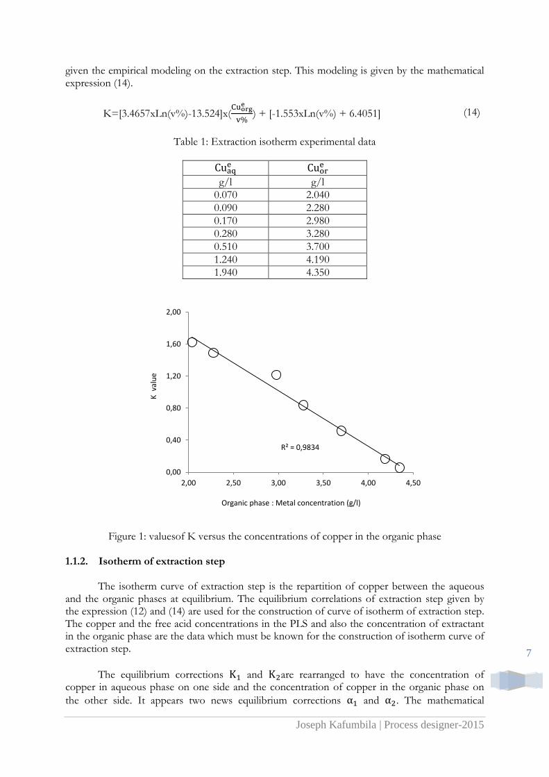
The chosen example from which the values of K obtained from the expression (12) are plotted on the graph versus the concentrations of copper in the organic phase at equilibrium is resumed in the BASF Redbook [4]. The initial aqueous phase contains 2.5 g/l of Copper at pH 1.8. The organic phase is constituted by 8.7 % of Lix 984N in Escaid 100. The initial organic phase contains 1.8 g/l of copper. Table 1 gives the concentrations of copper obtained in the laboratory in the organic and the aqueous phases at equilibrium. Figure 1 gives the value of K coming from expression (12) versus the concentration of copper in the organic phase. The results show that the value of K is the linear function of concentration of copper in the organic phase.
This linear thermodynamic property on extraction step is applied on the results obtained
in the laboratory with the extractant Lix 984N at different volume percentage of extractant and
Joseph Kafumbila | Process designer-2015
7
given the empirical modeling on the extraction step. This modeling is given by the mathematical expression (14).
K=[3.4657xLn(v%)-13.524]x(
) + [-1.553xLn(v%) + 6.4051] (14)
Table 1: Extraction isotherm experimental data
g/l g/l
0.070 2.040
0.090 2.280
0.170 2.980
0.280 3.280
0.510 3.700
1.240 4.190
1.940 4.350
Figure 1: valuesof K versus the concentrations of copper in the organic phase 1.1.2. Isotherm of extraction step
The isotherm curve of extraction step is the repartition of copper between the aqueous and the organic phases at equilibrium. The equilibrium correlations of extraction step given by the expression (12) and (14) are used for the construction of curve of isotherm of extraction step. The copper and the free acid concentrations in the PLS and also the concentration of extractant in the organic phase are the data which must be known for the construction of isotherm curve of extraction step.
The equilibrium corrections and are rearranged to have the concentration of copper in aqueous phase on one side and the concentration of copper in the organic phase on
the other side. It appears two news equilibrium corrections and . The mathematical
R² = 0,9834
0,00
0,40
0,80
1,20
1,60
2,00
2,00 2,50 3,00 3,50 4,00 4,50
K v
alu
e
Organic phase : Metal concentration (g/l)
Joseph Kafumbila | Process designer-2015
8
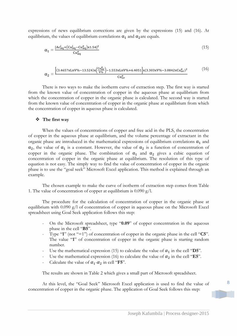
expressions of news equilibrium corrections are given by the expressions (15) and (16). At
equilibrium, the values of equilibrium correlations and are equals.
= [
(
) ]
(15)
= [ (
) ]
(16)
There is two ways to make the isotherm curve of extraction step. The first way is started
from the known value of concentration of copper in the aqueous phase at equilibrium from which the concentration of copper in the organic phase is calculated. The second way is started from the known value of concentration of copper in the organic phase at equilibrium from which the concentration of copper in aqueous phase is calculated.
The first way
When the values of concentrations of copper and free acid in the PLS, the concentration of copper in the aqueous phase at equilibrium, and the volume percentage of extractant in the
organic phase are introduced in the mathematical expressions of equilibrium correlations and
, the value of is a constant. However, the value of is a function of concentration of
copper in the organic phase. The combination of and gives a cubic equation of concentration of copper in the organic phase at equilibrium. The resolution of this type of equation is not easy. The simply way to find the value of concentration of copper in the organic phase is to use the “goal seek” Microsoft Excel application. This method is explained through an example.
The chosen example to make the curve of isotherm of extraction step comes from Table 1. The value of concentration of copper at equilibrium is 0.090 g/l.
The procedure for the calculation of concentration of copper in the organic phase at equilibrium with 0.090 g/l of concentration of copper in aqueous phase on the Microsoft Excel spreadsheet using Goal Seek application follows this step:
- On the Microsoft spreadsheet, type “0.09” of copper concentration in the aqueous phase in the cell “B5”.
- Type “1” (not “=1”) of concentration of copper in the organic phase in the cell “C5”. The value “1” of concentration of copper in the organic phase is starting random number.
- Use the mathematical expression (15) to calculate the value of in the cell “D5”.
- Use the mathematical expression (16) to calculate the value of in the cell “E5”.
- Calculate the value of - in cell “F5”.
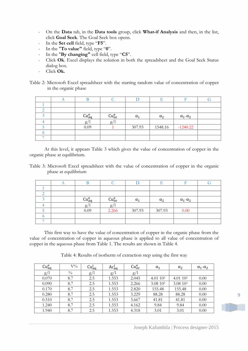
The results are shown in Table 2 which gives a small part of Microsoft spreadsheet.
At this level, the “Goal Seek” Microsoft Excel application is used to find the value of concentration of copper in the organic phase. The application of Goal Seek follows this step:
Joseph Kafumbila | Process designer-2015
9
- On the Data tab, in the Data tools group, click What-if Analysis and then, in the list, click Goal Seek. The Goal Seek box opens.
- In the Set cell field, type “F5”. - In the "To value" field, type “0”. - In the "By changing" cell field, type “C5”. - Click Ok. Excel displays the solution in both the spreadsheet and the Goal Seek Status
dialog box. - Click Ok.
Table 2: Microsoft Excel spreadsheet with the starting random value of concentration of copper
in the organic phase
A B C D E F G
1
2
3
-
4 g/l g/l
5 0.09 1 307.93 1548.16 -1240.22
6
7
At this level, it appears Table 3 which gives the value of concentration of copper in the
organic phase at equilibrium. Table 3: Microsoft Excel spreadsheet with the value of concentration of copper in the organic
phase at equilibrium
A B C D E F G
1
2
3
-
4 g/l g/l
5 0.09 2.266 307.93 307.93 0.00
6
7
This first way to have the value of concentration of copper in the organic phase from the
value of concentration of copper in aqueous phase is applied to all value of concentration of copper in the aqueous phase from Table 1. The results are shown in Table 4.
Table 4: Results of isotherm of extraction step using the first way
V%
-
g/l % g/l g/l g/l
0.070 8.7 2.5 1.553 2.045 4.01 102 4.01 102 0.00
0.090 8.7 2.5 1.553 2.266 3.08 102 3.08 102 0.00
0.170 8.7 2.5 1.553 2.820 155.48 155.48 0.00
0.280 8.7 2.5 1.553 3.229 88.28 88.28 0.00
0.510 8.7 2.5 1.553 3.667 41.81 41.81 0.00
1.240 8.7 2.5 1.553 4.162 9.84 9.84 0.00
1.940 8.7 2.5 1.553 4.318 3.01 3.01 0.00
Joseph Kafumbila | Process designer-2015
10
The second way
When the values of concentrations of copper and free acid in the PLS, the concentration of copper in the organic phase at equilibrium, and the volume percentage of extractant are
introduced in the mathematical expressions of equilibrium correlations and , the value of
is a constant. The value of is a function of concentration of copper in the aqueous phase.
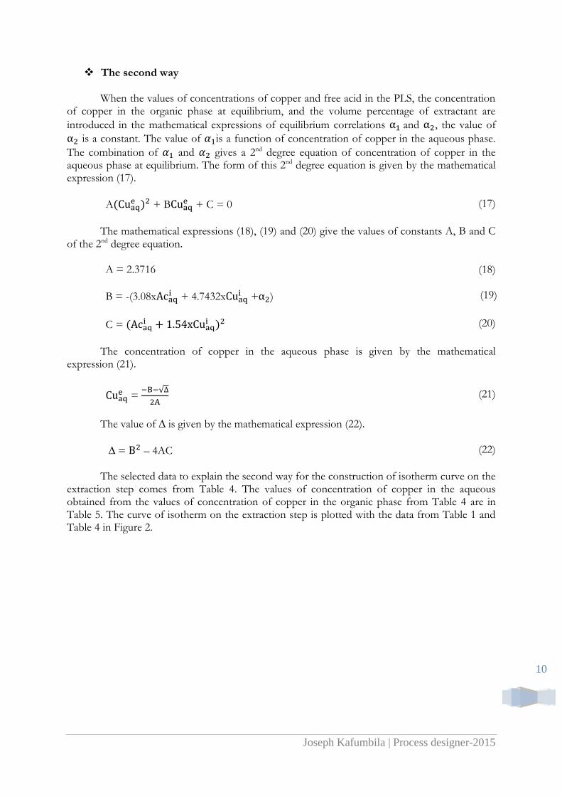
The combination of and gives a 2nd degree equation of concentration of copper in the aqueous phase at equilibrium. The form of this 2nd degree equation is given by the mathematical expression (17).
A + B
+ C = 0 (17)
The mathematical expressions (18), (19) and (20) give the values of constants A, B and C
of the 2nd degree equation.
A = 2.3716 (18)
B = -(3.08x + 4.7432x
+ ) (19)
C =
(20)
The concentration of copper in the aqueous phase is given by the mathematical
expression (21).
=
√
(21)
The value of ∆ is given by the mathematical expression (22).
∆ = – 4AC (22)
The selected data to explain the second way for the construction of isotherm curve on the
extraction step comes from Table 4. The values of concentration of copper in the aqueous obtained from the values of concentration of copper in the organic phase from Table 4 are in Table 5. The curve of isotherm on the extraction step is plotted with the data from Table 1 and Table 4 in Figure 2.
Joseph Kafumbila | Process designer-2015
11
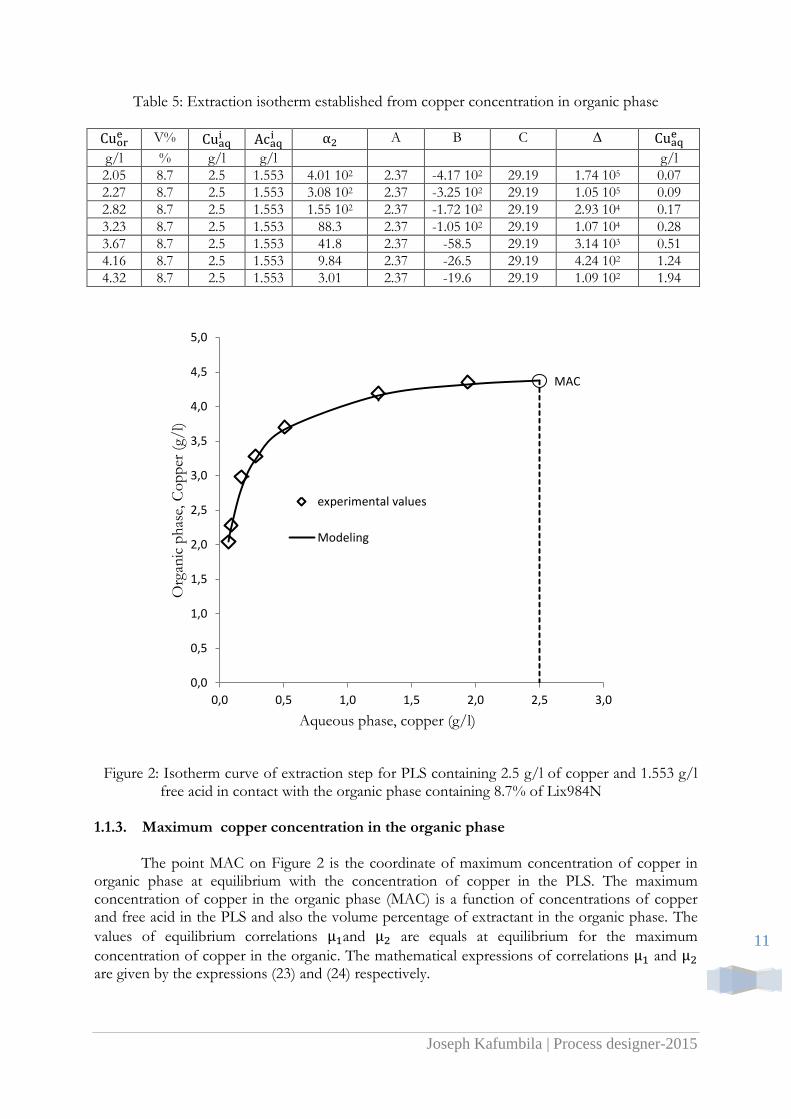
Table 5: Extraction isotherm established from copper concentration in organic phase
V%
A B C ∆
g/l % g/l g/l g/l
2.05 8.7 2.5 1.553 4.01 102 2.37 -4.17 102 29.19 1.74 105 0.07
2.27 8.7 2.5 1.553 3.08 102 2.37 -3.25 102 29.19 1.05 105 0.09
2.82 8.7 2.5 1.553 1.55 102 2.37 -1.72 102 29.19 2.93 104 0.17
3.23 8.7 2.5 1.553 88.3 2.37 -1.05 102 29.19 1.07 104 0.28
3.67 8.7 2.5 1.553 41.8 2.37 -58.5 29.19 3.14 103 0.51
4.16 8.7 2.5 1.553 9.84 2.37 -26.5 29.19 4.24 102 1.24
4.32 8.7 2.5 1.553 3.01 2.37 -19.6 29.19 1.09 102 1.94
Figure 2: Isotherm curve of extraction step for PLS containing 2.5 g/l of copper and 1.553 g/l free acid in contact with the organic phase containing 8.7% of Lix984N
1.1.3. Maximum copper concentration in the organic phase
The point MAC on Figure 2 is the coordinate of maximum concentration of copper in organic phase at equilibrium with the concentration of copper in the PLS. The maximum concentration of copper in the organic phase (MAC) is a function of concentrations of copper and free acid in the PLS and also the volume percentage of extractant in the organic phase. The
values of equilibrium correlations and are equals at equilibrium for the maximum
concentration of copper in the organic. The mathematical expressions of correlations and are given by the expressions (23) and (24) respectively.
MAC
0,0
0,5
1,0
1,5
2,0
2,5
3,0
3,5
4,0
4,5
5,0
0,0 0,5 1,0 1,5 2,0 2,5 3,0
Org
anic
ph
ase,
Co
pp
er (
g/l)
Aqueous phase, copper (g/l)
experimental values
Modeling
Joseph Kafumbila | Process designer-2015
12
=
x
(23)
= (3.4657xLn(V%)-13.524)x(
) +(-1.553xLn(V%)+6.4051) (24)
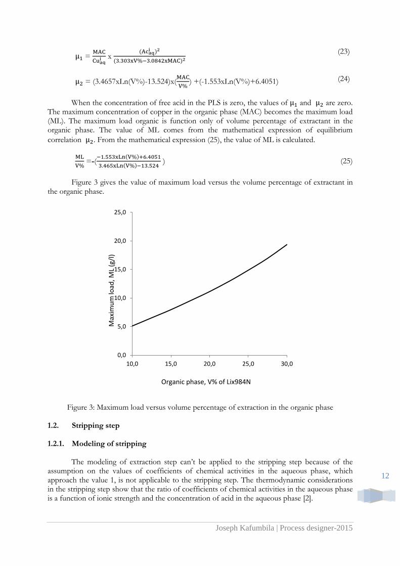
When the concentration of free acid in the PLS is zero, the values of and are zero. The maximum concentration of copper in the organic phase (MAC) becomes the maximum load (ML). The maximum load organic is function only of volume percentage of extractant in the organic phase. The value of ML comes from the mathematical expression of equilibrium
correlation . From the mathematical expression (25), the value of ML is calculated.
=-(
) (25)
Figure 3 gives the value of maximum load versus the volume percentage of extractant in
the organic phase.
Figure 3: Maximum load versus volume percentage of extraction in the organic phase 1.2. Stripping step 1.2.1. Modeling of stripping
The modeling of extraction step can’t be applied to the stripping step because of the assumption on the values of coefficients of chemical activities in the aqueous phase, which approach the value 1, is not applicable to the stripping step. The thermodynamic considerations in the stripping step show that the ratio of coefficients of chemical activities in the aqueous phase is a function of ionic strength and the concentration of acid in the aqueous phase [2].
0,0
5,0
10,0
15,0
20,0
25,0
10,0 15,0 20,0 25,0 30,0
Max
imu
m lo
ad, M
L (g
/l)
Organic phase, V% of Lix984N
Joseph Kafumbila | Process designer-2015
13
On the other hand, the results of isotherm curve on stripping step from laboratory show that the copper concentration in the organic phase is a linear function of ratio of concentrations of copper and free acid in the aqueous phase at equilibrium in the range of 30 to 60 g/l of copper and 140 to 200 g/l of free acid in the aqueous phase.
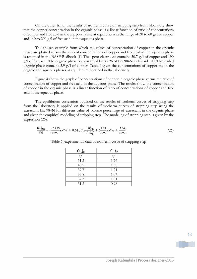
The chosen example from which the values of concentration of copper in the organic phase are plotted versus the ratio of concentrations of copper and free acid in the aqueous phase is resumed in the BASF Redbook [4]. The spent electrolyte contains 30.7 g/l of copper and 190 g/l of free acid. The organic phase is constituted by 8.7 % of Lix 984N in Escaid 100. The loaded organic phase contains 3.9 g/l of copper. Table 6 gives the concentrations of copper the in the organic and aqueous phases at equilibrium obtained in the laboratory.
Figure 4 shows the graph of concentrations of copper in organic phase versus the ratio of
concentration of copper and free acid in the aqueous phase. The results show the concentration of copper in the organic phase is a linear function of ratio of concentrations of copper and free acid in the aqueous phase.
The equilibrium correlation obtained on the results of isotherm curves of stripping step
from the laboratory is applied on the results of isotherm curves of stripping step using the extractant Lix 984N for different value of volume percentage of extractant in the organic phase and given the empirical modeling of stripping step. The modeling of stripping step is given by the expression (26).
= (
xV% + 0.6183)x(
) + (
xV% +
) (26)
Table 6: experimental data of isotherm curve of stripping step
g/l g/l
51.3 1.76
43.2 1.38
37.7 1.21
33.8 1.07
32.3 1.01
31.2 0.98
Joseph Kafumbila | Process designer-2015
14
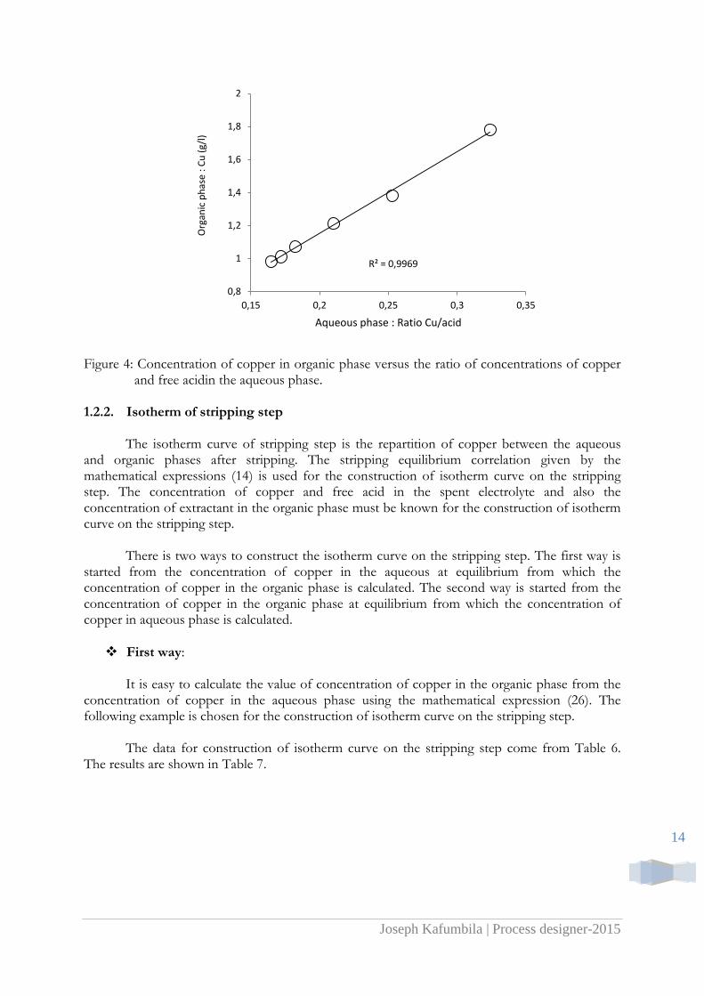
Figure 4: Concentration of copper in organic phase versus the ratio of concentrations of copper and free acidin the aqueous phase.
1.2.2. Isotherm of stripping step
The isotherm curve of stripping step is the repartition of copper between the aqueous and organic phases after stripping. The stripping equilibrium correlation given by the mathematical expressions (14) is used for the construction of isotherm curve on the stripping step. The concentration of copper and free acid in the spent electrolyte and also the concentration of extractant in the organic phase must be known for the construction of isotherm curve on the stripping step.
There is two ways to construct the isotherm curve on the stripping step. The first way is started from the concentration of copper in the aqueous at equilibrium from which the concentration of copper in the organic phase is calculated. The second way is started from the concentration of copper in the organic phase at equilibrium from which the concentration of copper in aqueous phase is calculated.
First way:
It is easy to calculate the value of concentration of copper in the organic phase from the concentration of copper in the aqueous phase using the mathematical expression (26). The following example is chosen for the construction of isotherm curve on the stripping step.
The data for construction of isotherm curve on the stripping step come from Table 6. The results are shown in Table 7.
R² = 0,9969
0,8
1
1,2
1,4
1,6
1,8
2
0,15 0,2 0,25 0,3 0,35
Org
anic
ph
ase
: Cu
(g/
l)
Aqueous phase : Ratio Cu/acid
Joseph Kafumbila | Process designer-2015
15
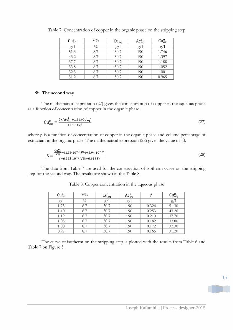
Table 7: Concentration of copper in the organic phase on the stripping step
V%
g/l % g/l g/l g/l
51.3 8.7 30.7 190 1.746
43.2 8.7 30.7 190 1.397
37.7 8.7 30.7 190 1.188
33.8 8.7 30.7 190 1.052
32.3 8.7 30.7 190 1.001
31.2 8.7 30.7 190 0.965
The second way
The mathematical expression (27) gives the concentration of copper in the aqueous phase as a function of concentration of copper in the organic phase.
=
(27)
where β is a function of concentration of copper in the organic phase and volume percentage of
extractant in the organic phase. The mathematical expression (28) gives the value of .
β =
(28)
The data from Table 7 are used for the construction of isotherm curve on the stripping
step for the second way. The results are shown in the Table 8.
Table 8: Copper concentration in the aqueous phase
V%
β
g/l % g/l g/l g/l
1.75 8.7 30.7 190 0.324 51.30
1.40 8.7 30.7 190 0.253 43.20
1.19 8.7 30.7 190 0.210 37.70
1.05 8.7 30.7 190 0.182 33.80
1.00 8.7 30.7 190 0.172 32.30
0.97 8.7 30.7 190 0.165 31.20
The curve of isotherm on the stripping step is plotted with the results from Table 6 and
Table 7 on Figure 5.
Joseph Kafumbila | Process designer-2015
16
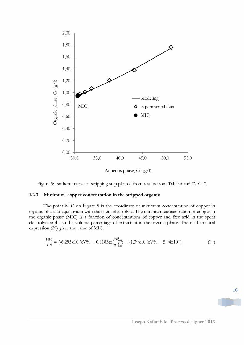
Figure 5: Isotherm curve of stripping step plotted from results from Table 6 and Table 7.
1.2.3. Minimum copper concentration in the stripped organic
The point MIC on Figure 5 is the coordinate of minimum concentration of copper in organic phase at equilibrium with the spent electrolyte. The minimum concentration of copper in the organic phase (MIC) is a function of concentrations of copper and free acid in the spent electrolyte and also the volume percentage of extractant in the organic phase. The mathematical expression (29) gives the value of MIC.
= (-6.295x10⁻³xV% + 0.6183)x(
) + (1.39x10⁻³xV% + 5.94x10⁻³) (29)
MIC
0,00
0,20
0,40
0,60
0,80
1,00
1,20
1,40
1,60
1,80
2,00
30,0 35,0 40,0 45,0 50,0 55,0
Org
anic
ph
ase,
Cu (
g/l)
Aqueous phase, Cu (g/l)
Modeling
experimental data
MIC

Joseph Kafumbila | Process designer-2015
17
2. Mass balance of copper solvent extraction 2.1. Scheme of stage on the extraction and the stripping step
The extraction and stripping steps of copper solvent are frequently carried out at industrial scale with the mixer-settlers. This equipment includes a mixer in one stage or two stages in series to disperse one phase into the other to provide interfacial contact for mass transfer, followed by the settler to allow the phases to coalesce and separate. Figure 6 and 7 give the scheme of stage of rank “n” on the extraction and the stripping steps in the cascade configuration.
Figure 6: The scheme of the stage “n” on the extraction step
The stage of rank “n” on the extraction step receives the aqueous phase from stage
of rank “n-1” and the organic phase from the stage of rank “n+1”. The stage of rank “n”
produces the aqueous phase and the organic phase
. In the extraction installation
containing “m” stages in cascade configuration, the stage of rank “1” receives the PLS ( ) and
produces the Loaded organic ( ). The last stage of rank “m” receives the stripped organic
( ) and produces the raffinate Raf (
).
Figure 7: The scheme of stage of rank “n” on the stripping stage step
The stage of rank “n” on stripping step receives the aqueous phase from stage of
rank “n+1” and the organic phase from stage of rank “n-1”. The stage of rank “n” produces
Sn
En
Joseph Kafumbila | Process designer-2015
18
the aqueous phase and the organic phase
. In the stripping installation containing “p”
stages in cascade configuration, the stage of rank “1” receives the loaded organic ( ) and
produces the advance electrolyte AD ( ). The last stage of rank “p” receives the spent
electrolyte SP (
) and produces the stripped organic (
).
2.2. Flow parameters of copper solvent extraction
Each aqueous phase leaving the stage of rank “n” on the extraction or the stripping step is characterized by the following independent parameters:
- = volumetric flow rate (m3/h).
- = concentration of copper (g/l).
- = concentration of free acid (g/l).
The mass flow rates of copper and free acid leaving the stage of rank “n” on the
extraction or the stripping step are given by the mathematical expressions (30) and (31) respectively.
=
x (kg/h) (30)
=
x (kg/h) (31)
Each organic phase leaving the stage of rank “n” on the extraction or the stripping step is
characterized by the following independent parameters:
- = volumetric flow rate (m3/h).
- = concentration of copper (g/l).
- = volume percentage of extractant in the organic phase (%).
The mass flow rate of copper leaving the stage of rank “n” on the extraction or the stripping is given by the mathematical expression (32).
=
x (kg/h) (32)
2.3. Equations of mass balance of copper solvent extraction 2.3.1. Extraction step
Stage of rank “n” on the extraction step On the extraction step, the mass balance equations are the following:
- The conservation of volumetric flow of aqueous phase at the stage of rank “n” is given
by the mathematical expression (33).
=
(33)
- The conservation of volumetric flow of organic phase at the stage of rank “n” is given by
the mathematical expression (34).
Joseph Kafumbila | Process designer-2015
19
=
(34)
- The conservation of volume percentage of extractant in the organic phase at the stage of
rank “n” is given by the mathematical expression (35).
= (35)
- The ratio of organic and aqueous flows at the stage of rank “n” is given by the
mathematical expression (36).
=
(36)
- The conservation of mass flow of copper at the stage of rank “n” is given by the
mathematical expression (37).
+
=
+
(37)
- The relation between the and the concentrations of copper in the inlet and outlet
flows of stage of rank “n” is given the mathematical expression (38).
=
(38)
- The value of free acid in outlet aqueous phase of stage of rank “n” is given the
mathematical expression (39).
=
+ ( -
)x1.54 (39)
- The extraction efficiency of copper of stage of rank “n” is given by the mathematical
expression (40).
=
x 100 (40)
cascade configuration
On the extraction step, the equations of mass balance in the cascade configuration containing “m” stages in series are the following:
- The conservation of volumetric flow of aqueous phase of cascade is given by the mathematical expression (41).
=
= =
= = (41)
- The conservation of volumetric flow of organic phase of cascade is given by the
mathematical expression (42).
=
= =
= = (42)
Joseph Kafumbila | Process designer-2015
20
- The conservation of volume percentage of extractant in the organic phase of cascade is given by the mathematical expression (43).
= = = = = (43)
- The ratio of organic and aqueous flows of cascade is given by the mathematical
expression (44).
=
= =
= = (44)
- The conservation of mass flow of copper of cascade is given by the mathematical
expression (45).
+
= +
(45)
- The relation between the and the concentrations of copper in the inlet and outlet
flows of cascade is given by the mathematical expression (46).
=
(46)
- The value of free acid in outlet aqueous phase of cascade is given by the mathematical
expression (47).
=
+ (PLS-Raf)x1.54 (47)
- The extraction efficiency of copper of cascade is given by the mathematical expression
(48).
=
x 100 (48)
2.3.2. Stripping step
stage of rank “n” of stripping step
On the stripping step, the equations of mass balance for the stage of rank “n” are the following:
- The conservation of volumetric flow of aqueous phase of stage of rank “n” is given by the mathematical expression (49).
=
(49)
- The conservation of volumetric flow of organic phase of stage of rank “n” is given by
the mathematical expression (50).
=
(50)
- The conservation of volume percentage of extractant in the organic phase of stage of
rank “n” is given by the mathematical expression (51).
Joseph Kafumbila | Process designer-2015
21
= (51)
- The ratio of organic and aqueous flows of stage of rank “n” is given by the mathematical
expression (52).
=
(52)
- The conservation of mass flow of copper of stage of rank “n” is given by the
mathematical expression (53).
+
=
+
(53)
- The relation between the and the concentrations of copper in the inlet and outlet
flows of stage of rank “n” is given by the mathematical expression (54).
=
(54)
- The value of free acid in outlet aqueous phase of stage of rank “n” is given by the
mathematical expression (55).
=
+ ( -
)x1.54 (55)
- The stripping efficiency of copper of stage of rank “n” is given by the mathematical
expression (56).
=
x 100 (56)
Cascade configuration
On the stripping step, the equations of mass balance of cascade configuration containing “p” stages in series are the following:
- The conservation of volumetric flow of aqueous phase of cascade is given by the
mathematical expression (57).
= =
= = =
(57)
- The conservation of volumetric flow of organic phase of cascade is given by the
mathematical expression (58).
= =
= = =
(58)
- The conservation of volume percentage of extractant in the organic phase of cascade is
given by the mathematical expression (59).
= = = = = (59)
Joseph Kafumbila | Process designer-2015
22
- The ratio of organic flow and aqueous flow of cascade is given by the mathematical expression (60).
= =
= = =
(60)
- The conservation of mass flow of copper of cascade is given by the mathematical
expression (61).
+
=
+
(61)
- The relation between the and the concentrations of copper in the inlet and outlet
flows of cascade is given by the mathematical expression (62).
=
(62)
- The value of free acid in outlet aqueous phase of cascade is given by the mathematical
expression (63).
=
+ (
-
)x1.54 (63)
- The stripping efficiency of copper of cascade is given by the mathematical expression
(64).
=
x 100 (64)
- The copper transfer from organic phase to the aqueous phase is given by the
mathematical expression (65).
=
(g/l Cu/1%V%) (65)
2.3.3. Equilibrium constraints between the extraction and the stripping steps
In solvent extraction installation having the extraction step containing one or more cascades and the stripping step containing one or more cascades, the equilibrium constraints between extraction and stripping steps are given by the mathematical expressions (66) and (67).
= (66)
= (67)
2.4. Mixing efficiency 2.4.1. Description of mixing efficiency
In the industrial installation of copper solvent extraction, the copper concentrations out
of mixer on the extraction and the stripping stage in the aqueous and organic phases are not at equilibrium. This phenomenon is due to the temperature, the residence time in the mixer, the model of impeller, the impeller power, the percentage of extractant in the organic phase, the
Joseph Kafumbila | Process designer-2015
23
presence of iron, the solution viscosity, the ratio O/A in the mixer, the quality of extractant and the concentration of copper in the organic phase [5]. 2.4.2. Flow parameters
Each aqueous phase leaving the extraction or the stripping stage of rank “n” is characterized by the following independent parameters:
- = volumetric flow rate (m3/h).
- = concentration of copper (g/l).
- = concentration of free acid (g/l).
- = concentration of copper at equilibrium (g/l).
- = concentration of free acid at equilibrium (g/).
- = mixing efficiency (%).
Each organic phase leaving the extraction or the stripping stage of rank “n” is
characterized by the following independent parameters:
- = volumetric flow rate (m3/h).
- = concentration of copper (g/l).
- = concentration of copper at equilibrium (g/l).
- = mixing efficiency (%).
- = volume percentage of extractant in the organic phase (%).
2.4.3. Correlations of concentrations of copper
Extraction step
On the extraction step, the concentrations of copper in the aqueous and organic phases leaving the stage of rank “n” are given by the mathematical expressions (68) and (69).
=
x
+
x(1-
) (68)
=
x
+
x(1-
) (69)
Stripping step
On the stripping step at stage of rank “n”, the concentrations of copper in the aqueous and organic phases leaving the stage of rank “n” are given by the mathematical expressions (70) and (71).
=
x
+
x(1-
) (70)
=
x
+
x(1-
) (71)
Joseph Kafumbila | Process designer-2015
24
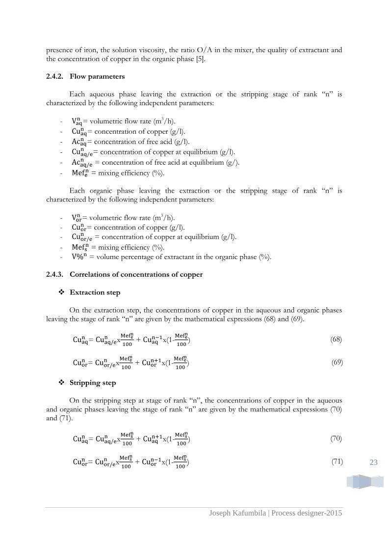
2.4.4. Industrial data of mixing efficiency Table 9 gives the industrial values of mixing efficiency of different stage on the extraction
and the stripping steps. This measurement has been done on the North America solvent extraction plant [6].
Table 8: Industrial mixing efficiency at different stages
Stage Mixing efficiency (%) 92±2 94 2 97±2 ≥98 ≥98
2.5. MacCabe Thiele diagram
2.5.1. Extraction step
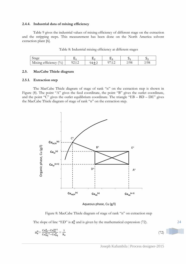
The MacCabe Thiele diagram of stage of rank “n” on the extraction step is shown in
Figure (8). The point “A” gives the feed coordinate, the point “B” gives the outlet coordinate, and the point “C” gives the outlet equilibrium coordinate. The triangle “EB – BD – DE” gives the MacCabe Thiele diagram of stage of rank “n” on the extraction step.
Figure 8: MacCabe Thiele diagram of stage of rank “n” on extraction step
The slope of line “ED” is and is given by the mathematical expression (72).
=
=
(72)
An
Cn
Cuor/e(n)
En
Cuor(n)
Cuor(n+1)
Cuaq/e(n) Cuaq
(n) Cuaq(n-1)
Bn
Dn
Org
anic
ph
ase,
Cu
(g/
l)
Aqueous phase, Cu (g/l)
Joseph Kafumbila | Process designer-2015
25
The slope of line “AB” is and is given by the mathematical expression (73).
=
= -
(73)
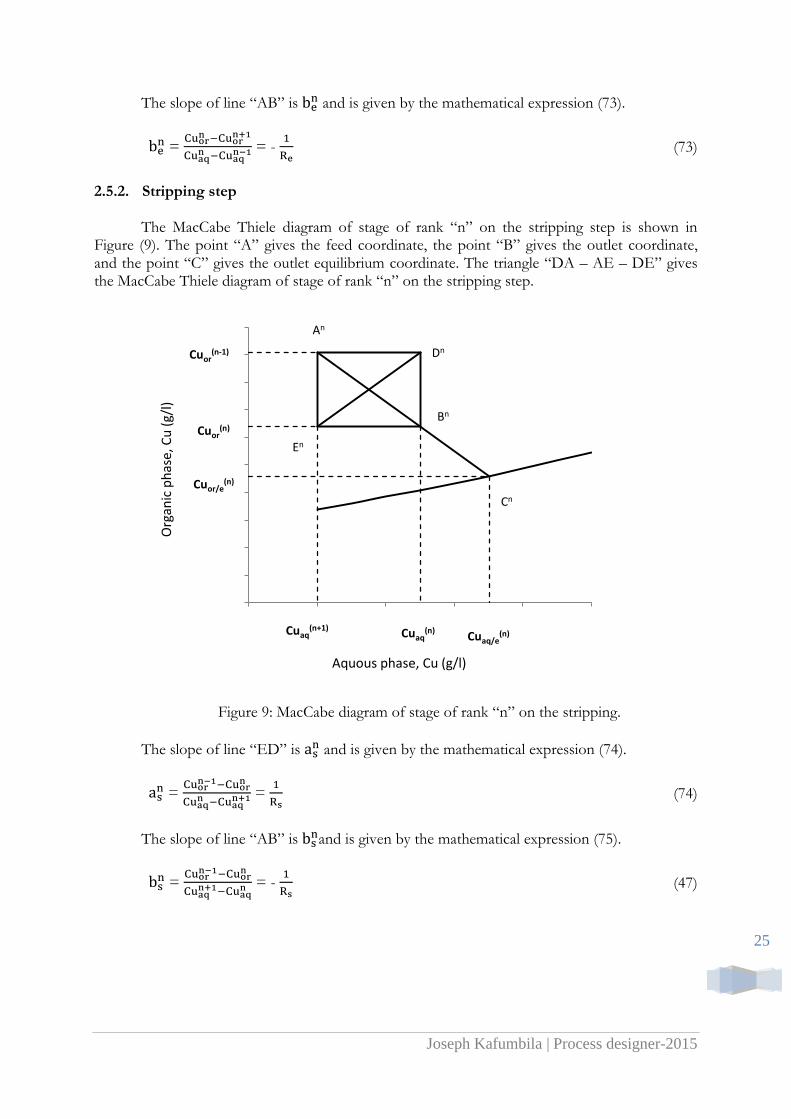
2.5.2. Stripping step
The MacCabe Thiele diagram of stage of rank “n” on the stripping step is shown in
Figure (9). The point “A” gives the feed coordinate, the point “B” gives the outlet coordinate, and the point “C” gives the outlet equilibrium coordinate. The triangle “DA – AE – DE” gives the MacCabe Thiele diagram of stage of rank “n” on the stripping step.
Figure 9: MacCabe diagram of stage of rank “n” on the stripping.
The slope of line “ED” is and is given by the mathematical expression (74).
=
=
(74)
The slope of line “AB” is and is given by the mathematical expression (75).
=
= -
(47)
An
Bn
Cn
Dn
En
Cuaq(n+1) Cuaq
(n) Cuaq/e
(n)
Cuor(n-1)
Cuor(n)
Cuor/e(n)
Org
anic
ph
ase,
Cu
(g/
l)
Aquous phase, Cu (g/l)
Joseph Kafumbila | Process designer-2015
26
3. Simulation of solvent extraction scheme
3.1. Constraints of copper SX/EW configuration
The constraints of copper SX/EW come from the copper solvent extraction configuration as well as the industrial practices.
3.1.1. Maximum value of V% in the organic phase
The organic phase is constituted with the extractant and the diluent. The extractant is Lix
984N which is the mixing of 50% of 2-hydroxy-5-nonylacetophenone oxime and 50% of 5-nonylasalcylaldoxime. The diluents are the organic liquid in which the extractant is dissolved. The diluents are the hydrocarbons.
The viscosity of organic phase increases with increasing of volume percentage of
extractant. In the industrial practices, the maximum value of volume percentage of extractant in the organic phase is 30 – 33% [7].
3.1.2. PLS and spent electrolyte temperature
The PLS temperature is a function of leaching technique. The temperature of PLS
coming from in situ leaching, heap leaching and vat leaching is generally less than 40°C. The temperature of PLS coming from agitated leach of oxide ores can reach 50°C because of the chemical reaction and the dilution of sulphuric acid in water are exothermic. In all case, the temperature of PLS is less than 40°C after storage in the pond.
The temperature of spent electrolyte out of EW is around 50°C. The heat-exchanger is
placed on the spent electrolyte to transfer the heat from the spent electrolyte to the advance electrolyte before the stripping step.
The temperature has not any effect on the thermodynamic and the kinetic of copper
solvent extraction.
3.1.3. Free acid concentration in the PLS
The concentration of free acid in the PLS is a function of leaching technique [6]. Table 9 gives the level of free acid in the outlet of leaching circuit.
Table 9: Concentration of free acid in the outlet leaching circuit Leaching techniques Free acid (g/l) pH
In situ leaching 0,5 - 8 1,3 – 2,2
Heap leaching 3 - 8 1,5 – 2,2
Vat leaching 6 - 40 1,5 – 2,0
Oxide agitated leaching 1 - 15 1,5 – 2,0
Sulphide agitated leaching 12 - 25 <1 – 1,6
Autoclave 25 - 80 <1 – 2,0
Bacterial leaching 25 - 55 <1 – 2,2
Joseph Kafumbila | Process designer-2015
27
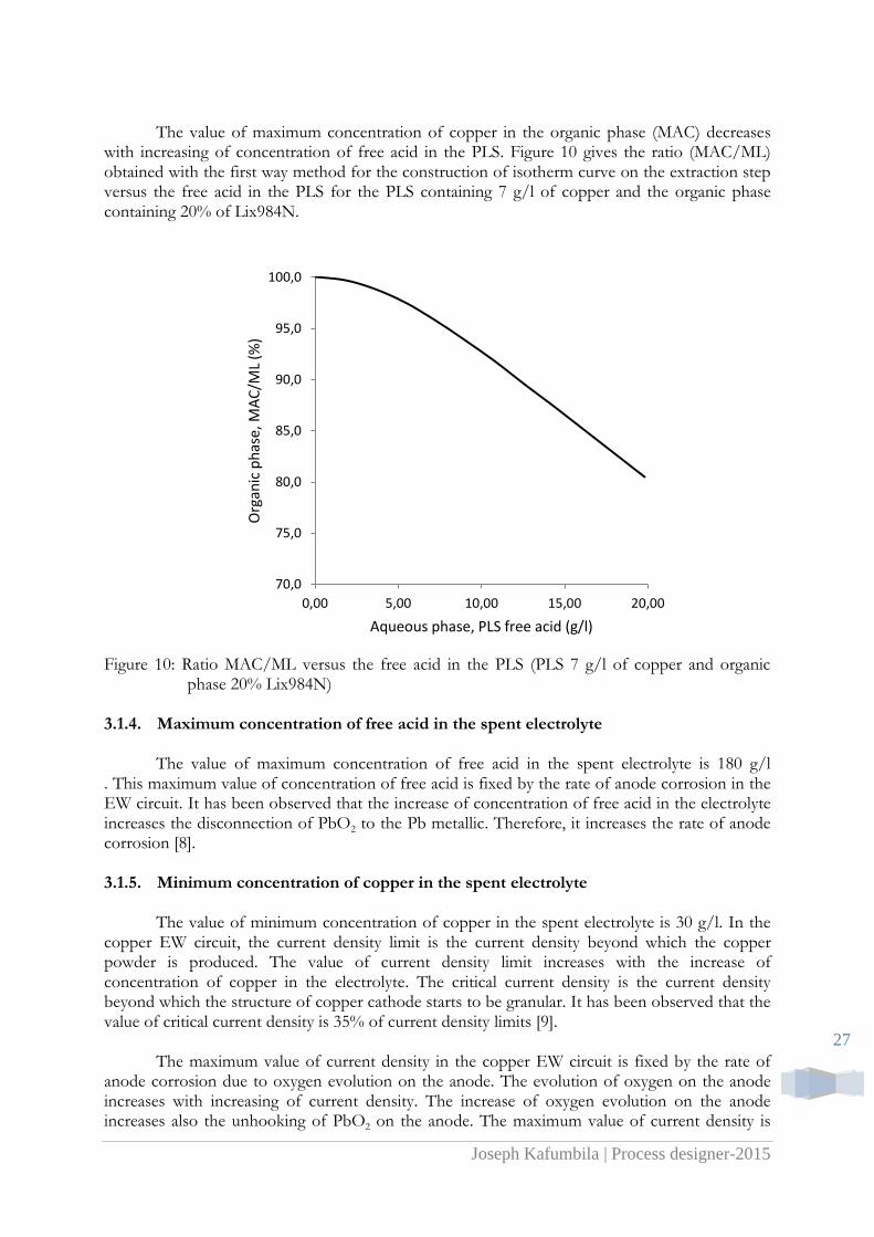
The value of maximum concentration of copper in the organic phase (MAC) decreases
with increasing of concentration of free acid in the PLS. Figure 10 gives the ratio (MAC/ML) obtained with the first way method for the construction of isotherm curve on the extraction step versus the free acid in the PLS for the PLS containing 7 g/l of copper and the organic phase containing 20% of Lix984N.
Figure 10: Ratio MAC/ML versus the free acid in the PLS (PLS 7 g/l of copper and organic
phase 20% Lix984N)
3.1.4. Maximum concentration of free acid in the spent electrolyte The value of maximum concentration of free acid in the spent electrolyte is 180 g/l
. This maximum value of concentration of free acid is fixed by the rate of anode corrosion in the EW circuit. It has been observed that the increase of concentration of free acid in the electrolyte increases the disconnection of PbO2 to the Pb metallic. Therefore, it increases the rate of anode corrosion [8].
3.1.5. Minimum concentration of copper in the spent electrolyte
The value of minimum concentration of copper in the spent electrolyte is 30 g/l. In the
copper EW circuit, the current density limit is the current density beyond which the copper powder is produced. The value of current density limit increases with the increase of concentration of copper in the electrolyte. The critical current density is the current density beyond which the structure of copper cathode starts to be granular. It has been observed that the value of critical current density is 35% of current density limits [9].
The maximum value of current density in the copper EW circuit is fixed by the rate of
anode corrosion due to oxygen evolution on the anode. The evolution of oxygen on the anode increases with increasing of current density. The increase of oxygen evolution on the anode increases also the unhooking of PbO2 on the anode. The maximum value of current density is
70,0
75,0
80,0
85,0
90,0
95,0
100,0
0,00 5,00 10,00 15,00 20,00
Org
anic
ph
ase,
MA
C/M
L (%
)
Aqueous phase, PLS free acid (g/l)
Joseph Kafumbila | Process designer-2015
28
320 A/m2. This value allows to the anodes to have a life of 5 years. The value of maximum current density must be lower than the critical current density of the concentration of copper in the spent electrolyte. It has been observed that the minimum value of copper concentration in the spent electrolyte which respects this constraint is 30 g/l. In the industrial practice, the value of copper in the spent electrolyte is 35 g/l.
3.1.6. Maximum concentration of copper in the advance electrolyte
In the past time, the /
ratio was fixed. This ratio is the enrichment factor of concentration of copper from the leach solution and to the electrolyte. Under these conditions, the concentration of copper in advance electrolyte increases with increasing the amount of copper transferred. The maximum concentration of copper in the advance electrolyte is reached when the LO/MAC ratio is 100%. The amperage of current to the EW was adjusted depending on the concentration of copper in advance electrolyte.
Currently, the copper tank house is designed to work at the maximum level of the current amperage. For a conventional cell containing 75 cathodes, the flow rate of the electrolyte is increased to reach 15 m3/h. The increase in the cell flow rate is for a better quality of surface of cathodes. The copper tank house consists of two parts; the first part, called scavenger cell, is treating the advance electrolyte to oxidize the soluble organic phase coming with advance electrolyte. The second part, called commercial cell, is treating the mixture of the outlet solution of cell scavenger and the recycled solution outlet of same part. Accordingly, the copper concentration gradient across the cell is 3 g/l. The design of copper tank house is done such as the flow rate of electrolyte to the commercial cells is 4 times greater than the advance flow rate of the electrolyte to the scavenger cells. Under these conditions, the maximum gradient of the copper concentration between the spent and advance electrolytes is 15 g/l and for a copper concentration in the spent electrolyte of 35 g/l, the maximum concentration of copper in the advance electrolyte is 50 g/l.
Also note that increasing the concentration of copper in the advance electrolyte increases the
concentration of copper in the stripped organic phase and decreases the copper extraction efficiency.
3.1.7. Minimum value of
The minimum value of is reached when the value of is reached the value of
MAC. The extraction is stopped. Therefore, the values of concentration of copper in the PLS
and in the raffinate are the same. The value of is zero.
At a given value of LO/MAC lower than 100%, the value of increases with decreasing
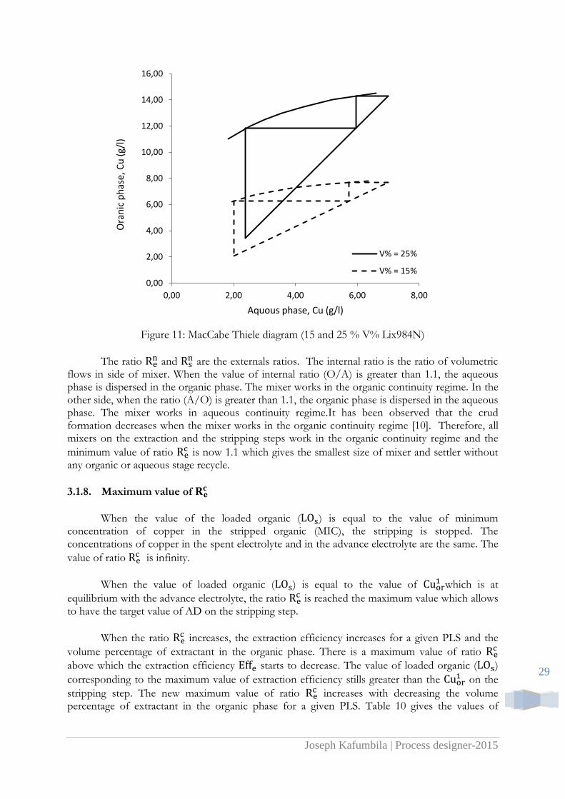
the value of volume percentage of extractant in the organic phase for a given PLS. Figure 11 gives the MacCabe Thiele diagrams on the extraction step of Copper SX having 15 and 25 % of volume percentage of extraction after the simulation of copper SX working with the conventional configuration 2Ex2S. The PLS has 7g/l of copper and 4 g/l of free acid. The spent electrolyte has 35 g/l of copper and 180 g/l of free acid. The advance electrolyte has 50 g/l of copper. The values of mixing efficiency for all mixers are 100%. The extractant is Lix984N. The value of LO/MAC is 98%.
Joseph Kafumbila | Process designer-2015
29
Figure 11: MacCabe Thiele diagram (15 and 25 % V% Lix984N)
The ratio and
are the externals ratios. The internal ratio is the ratio of volumetric flows in side of mixer. When the value of internal ratio (O/A) is greater than 1.1, the aqueous phase is dispersed in the organic phase. The mixer works in the organic continuity regime. In the other side, when the ratio (A/O) is greater than 1.1, the organic phase is dispersed in the aqueous phase. The mixer works in aqueous continuity regime.It has been observed that the crud formation decreases when the mixer works in the organic continuity regime [10]. Therefore, all mixers on the extraction and the stripping steps work in the organic continuity regime and the
minimum value of ratio is now 1.1 which gives the smallest size of mixer and settler without
any organic or aqueous stage recycle.
3.1.8. Maximum value of
When the value of the loaded organic ( ) is equal to the value of minimum concentration of copper in the stripped organic (MIC), the stripping is stopped. The concentrations of copper in the spent electrolyte and in the advance electrolyte are the same. The
value of ratio is infinity.
When the value of loaded organic ( ) is equal to the value of which is at
equilibrium with the advance electrolyte, the ratio is reached the maximum value which allows
to have the target value of AD on the stripping step.
When the ratio increases, the extraction efficiency increases for a given PLS and the
volume percentage of extractant in the organic phase. There is a maximum value of ratio
above which the extraction efficiency starts to decrease. The value of loaded organic ( )
corresponding to the maximum value of extraction efficiency stills greater than the on the
stripping step. The new maximum value of ratio increases with decreasing the volume
percentage of extractant in the organic phase for a given PLS. Table 10 gives the values of
0,00
2,00
4,00
6,00
8,00
10,00
12,00
14,00
16,00
0,00 2,00 4,00 6,00 8,00
Ora
nic
ph
ase,
Cu
(g/
l)
Aquous phase, Cu (g/l)
V% = 25%
V% = 15%
Joseph Kafumbila | Process designer-2015
30
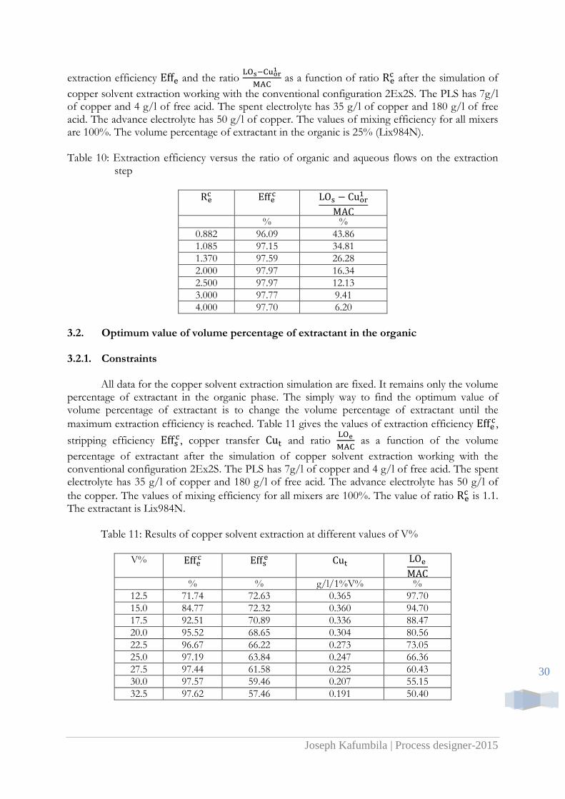
extraction efficiency and the ratio
as a function of ratio
after the simulation of
copper solvent extraction working with the conventional configuration 2Ex2S. The PLS has 7g/l of copper and 4 g/l of free acid. The spent electrolyte has 35 g/l of copper and 180 g/l of free acid. The advance electrolyte has 50 g/l of copper. The values of mixing efficiency for all mixers are 100%. The volume percentage of extractant in the organic is 25% (Lix984N).
Table 10: Extraction efficiency versus the ratio of organic and aqueous flows on the extraction
step
% %
0.882 96.09 43.86
1.085 97.15 34.81
1.370 97.59 26.28
2.000 97.97 16.34
2.500 97.97 12.13
3.000 97.77 9.41
4.000 97.70 6.20
3.2. Optimum value of volume percentage of extractant in the organic 3.2.1. Constraints
All data for the copper solvent extraction simulation are fixed. It remains only the volume
percentage of extractant in the organic phase. The simply way to find the optimum value of volume percentage of extractant is to change the volume percentage of extractant until the
maximum extraction efficiency is reached. Table 11 gives the values of extraction efficiency ,
stripping efficiency , copper transfer and ratio
as a function of the volume
percentage of extractant after the simulation of copper solvent extraction working with the conventional configuration 2Ex2S. The PLS has 7g/l of copper and 4 g/l of free acid. The spent electrolyte has 35 g/l of copper and 180 g/l of free acid. The advance electrolyte has 50 g/l of
the copper. The values of mixing efficiency for all mixers are 100%. The value of ratio is 1.1.
The extractant is Lix984N. Table 11: Results of copper solvent extraction at different values of V%
V%
% % g/l/1%V% %
12.5 71.74 72.63 0.365 97.70
15.0 84.77 72.32 0.360 94.70
17.5 92.51 70.89 0.336 88.47
20.0 95.52 68.65 0.304 80.56
22.5 96.67 66.22 0.273 73.05
25.0 97.19 63.84 0.247 66.36
27.5 97.44 61.58 0.225 60.43
30.0 97.57 59.46 0.207 55.15
32.5 97.62 57.46 0.191 50.40
Joseph Kafumbila | Process designer-2015
31
The results show that the extraction efficiency increases with increasing of volume percentage of extraction in the organic phase. In the other side, the stripping efficiency, the copper transfer, and the ratio LO/MAC decrease with increasing of volume percentage of extractant in the organic.
In the old time, the choice of optimum was based on the high value of extraction
efficiency. Actually, the choice is based on the organic phase saturation with the copper. 3.2.2. Maximum extraction efficiency
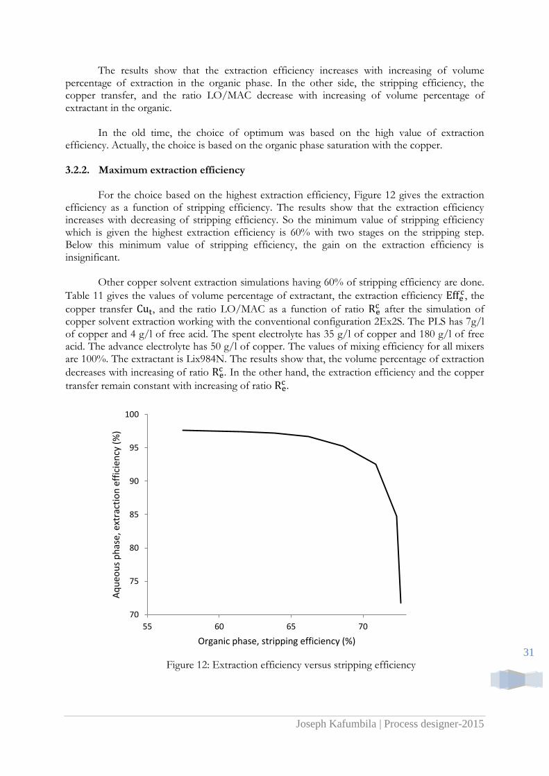
For the choice based on the highest extraction efficiency, Figure 12 gives the extraction efficiency as a function of stripping efficiency. The results show that the extraction efficiency increases with decreasing of stripping efficiency. So the minimum value of stripping efficiency which is given the highest extraction efficiency is 60% with two stages on the stripping step. Below this minimum value of stripping efficiency, the gain on the extraction efficiency is insignificant.
Other copper solvent extraction simulations having 60% of stripping efficiency are done.
Table 11 gives the values of volume percentage of extractant, the extraction efficiency , the
copper transfer , and the ratio LO/MAC as a function of ratio after the simulation of
copper solvent extraction working with the conventional configuration 2Ex2S. The PLS has 7g/l of copper and 4 g/l of free acid. The spent electrolyte has 35 g/l of copper and 180 g/l of free acid. The advance electrolyte has 50 g/l of copper. The values of mixing efficiency for all mixers are 100%. The extractant is Lix984N. The results show that, the volume percentage of extraction
decreases with increasing of ratio . In the other hand, the extraction efficiency and the copper
transfer remain constant with increasing of ratio .
Figure 12: Extraction efficiency versus stripping efficiency
70
75
80
85
90
95
100
55 60 65 70
Aq
ueo
us
ph
ase,
ext
ract
ion
eff
icie
ncy
(%
)
Organic phase, stripping efficiency (%)
Joseph Kafumbila | Process designer-2015
32
Table 12: Results of copper solvent extraction simulation with 60% of stripping efficiency
% % g/l/1%V% %
1.1 29.34 97.55 0.212 56.49
1.3 24.74 97.51 0.212 60.79
1.5 21.37 97.42 0.213 63.58
1.7 18.79 97.30 0.213 65.47
1.9 16.76 97.16 0.214 66.81
3.2.3. Saturation of organic phase with the copper
The ferric is the only impurity which can be transferred to the copper electrolyte by
chemical and physical entrainment. In the normal copper solvent plant working together with the normal leaching technique of oxide ores, the chemical entrainment of iron is between 35 to 60% of total entrainment [11]. The presence of iron in the copper electrolyte causes the reduction of current efficiency. The maximum concentration of iron in the copper electrolyte is 2g/l. The bleed of copper electrolyte is applied to maintain the iron concentration in the copper electrolyte at less than 2 g/l. The increase of the flow rate of copper electrolyte bleed increases the cost of cobalt reagent which is added to the copper EW circuit.
In all copper solvent extraction plants working in cascade configuration with two stages
on the extraction step, it has been observed that the concentration of iron in the partial loaded organic out of stage 2 is greater than the concentration of iron in the loaded organic out of stage 1. This effect is called “crowding” [11].
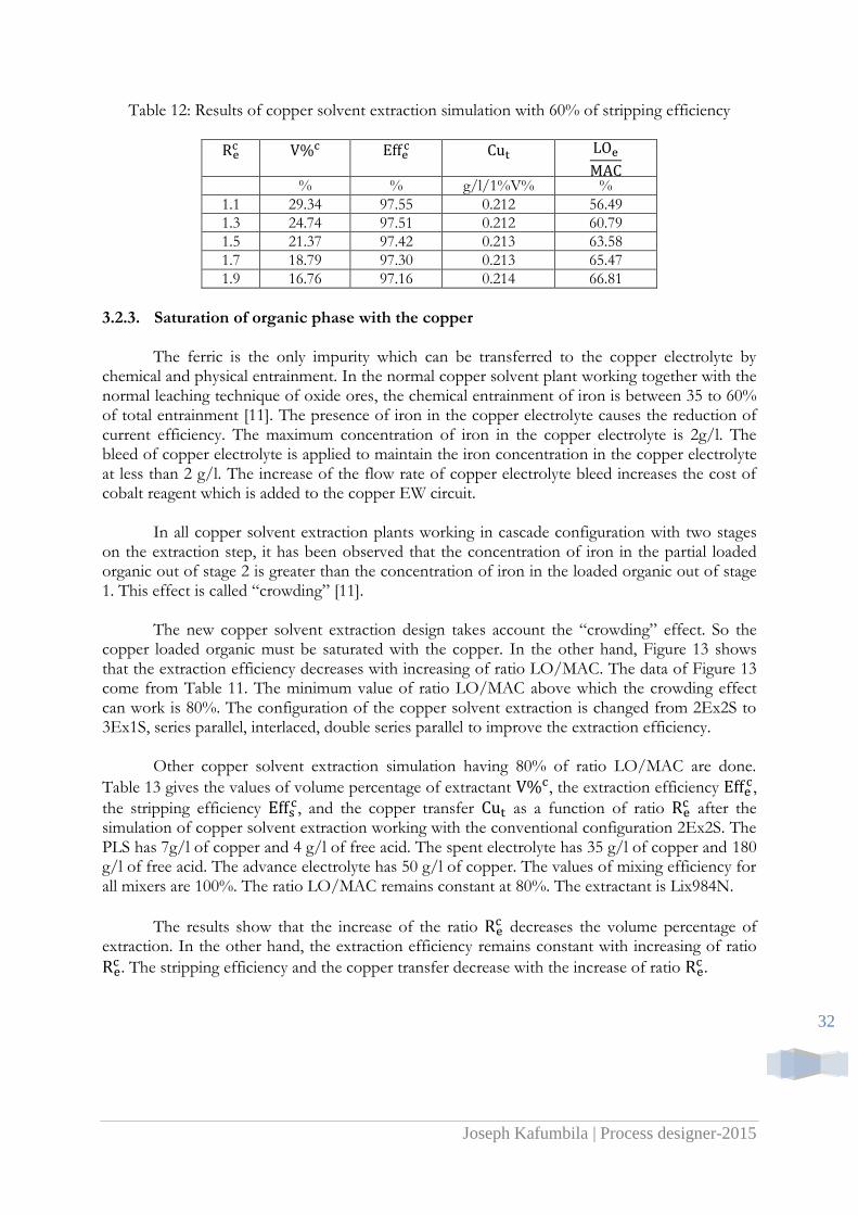
The new copper solvent extraction design takes account the “crowding” effect. So the
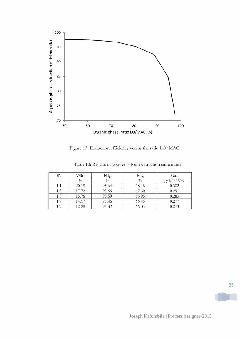
copper loaded organic must be saturated with the copper. In the other hand, Figure 13 shows that the extraction efficiency decreases with increasing of ratio LO/MAC. The data of Figure 13 come from Table 11. The minimum value of ratio LO/MAC above which the crowding effect can work is 80%. The configuration of the copper solvent extraction is changed from 2Ex2S to 3Ex1S, series parallel, interlaced, double series parallel to improve the extraction efficiency.
Other copper solvent extraction simulation having 80% of ratio LO/MAC are done.
Table 13 gives the values of volume percentage of extractant , the extraction efficiency ,
the stripping efficiency , and the copper transfer as a function of ratio
after the simulation of copper solvent extraction working with the conventional configuration 2Ex2S. The PLS has 7g/l of copper and 4 g/l of free acid. The spent electrolyte has 35 g/l of copper and 180 g/l of free acid. The advance electrolyte has 50 g/l of copper. The values of mixing efficiency for all mixers are 100%. The ratio LO/MAC remains constant at 80%. The extractant is Lix984N.
The results show that the increase of the ratio decreases the volume percentage of
extraction. In the other hand, the extraction efficiency remains constant with increasing of ratio
. The stripping efficiency and the copper transfer decrease with the increase of ratio
.
Joseph Kafumbila | Process designer-2015
33
Figure 13: Extraction efficiency versus the ratio LO/MAC
Table 13: Results of copper solvent extraction simulation
% % % g/l/1%V%
1.1 20.18 95.64 68.48 0.302
1.3 17.72 95.66 67.60 0.291
1.5 15.76 95.59 66.95 0.283
1.7 14.17 95.46 66.45 0.277
1.9 12.88 95.32 66.03 0.273
70
75
80
85
90
95
100
50 60 70 80 90 100
Aq
ueo
us
ph
ase,
ext
ract
ion
eff
icie
ncy
(%
)
Organic phase, ratio LO/MAC (%)
Joseph Kafumbila | Process designer-2015
34
3.3. Procedure of copper solvent extraction simulation
3.3.1. Plant description
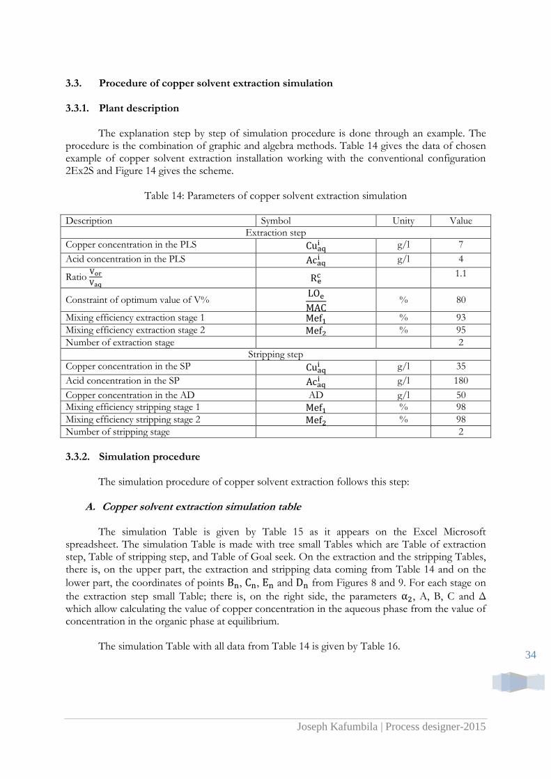
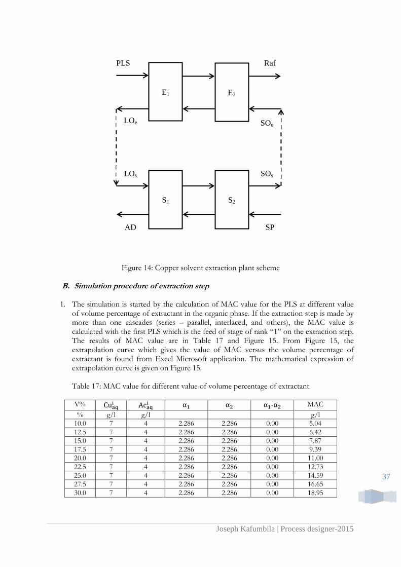
The explanation step by step of simulation procedure is done through an example. The procedure is the combination of graphic and algebra methods. Table 14 gives the data of chosen example of copper solvent extraction installation working with the conventional configuration 2Ex2S and Figure 14 gives the scheme.
Table 14: Parameters of copper solvent extraction simulation Description Symbol Unity Value
Extraction step
Copper concentration in the PLS g/l 7
Acid concentration in the PLS g/l 4
Ratio
1.1
Constraint of optimum value of V%
% 80
Mixing efficiency extraction stage 1 % 93
Mixing efficiency extraction stage 2 % 95
Number of extraction stage 2
Stripping step
Copper concentration in the SP g/l 35
Acid concentration in the SP g/l 180
Copper concentration in the AD AD g/l 50
Mixing efficiency stripping stage 1 % 98
Mixing efficiency stripping stage 2 % 98
Number of stripping stage 2
3.3.2. Simulation procedure
The simulation procedure of copper solvent extraction follows this step:
A. Copper solvent extraction simulation table
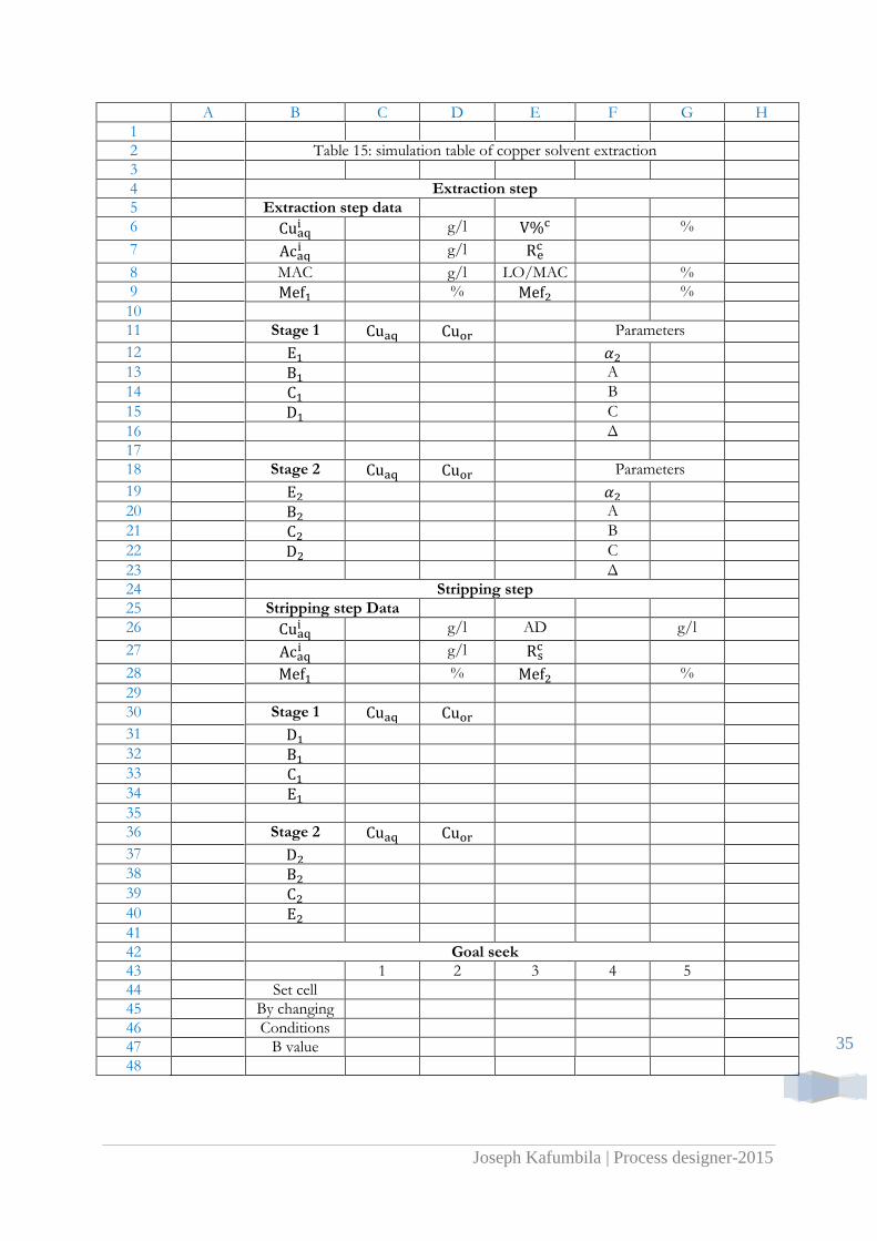
The simulation Table is given by Table 15 as it appears on the Excel Microsoft spreadsheet. The simulation Table is made with tree small Tables which are Table of extraction step, Table of stripping step, and Table of Goal seek. On the extraction and the stripping Tables, there is, on the upper part, the extraction and stripping data coming from Table 14 and on the
lower part, the coordinates of points , , and from Figures 8 and 9. For each stage on
the extraction step small Table; there is, on the right side, the parameters , A, B, C and Δ which allow calculating the value of copper concentration in the aqueous phase from the value of concentration in the organic phase at equilibrium.
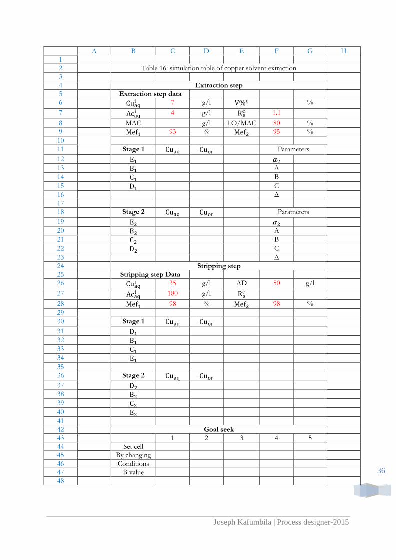
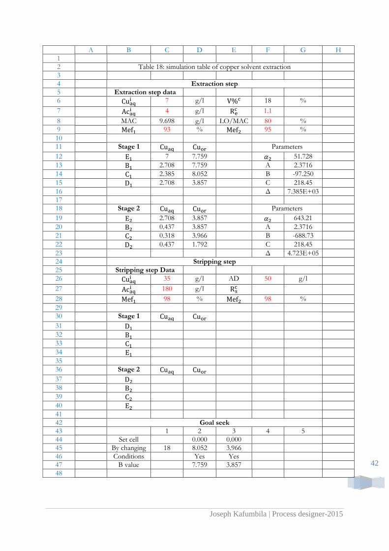
The simulation Table with all data from Table 14 is given by Table 16.
Joseph Kafumbila | Process designer-2015
35
A B C D E F G H
1
2 Table 15: simulation table of copper solvent extraction
3
4 Extraction step
5 Extraction step data
6 g/l %
7 g/l
8 MAC g/l LO/MAC %
9 % %
10
11 Stage 1 Parameters
12
13 A
14 B
15 C
16 Δ
17
18 Stage 2 Parameters
19
20 A
21 B
22 C
23 Δ
24 Stripping step
25 Stripping step Data
26 g/l AD g/l
27 g/l
28 % %
29
30 Stage 1
31
32
33
34
35
36 Stage 2
37
38
39
40
41
42 Goal seek
43 1 2 3 4 5
44 Set cell
45 By changing
46 Conditions
47 B value
48
Joseph Kafumbila | Process designer-2015
36
A B C D E F G H
1
2 Table 16: simulation table of copper solvent extraction
3
4 Extraction step
5 Extraction step data
6 7 g/l %
7 4 g/l
1.1
8 MAC g/l LO/MAC 80 %
9 93 % 95 %
10
11 Stage 1 Parameters
12
13 A
14 B
15 C
16 Δ
17
18 Stage 2 Parameters
19
20 A
21 B
22 C
23 Δ
24 Stripping step
25 Stripping step Data
26 35 g/l AD 50 g/l
27 180 g/l
28 98 % 98 %
29
30 Stage 1
31
32
33
34
35
36 Stage 2
37
38
39
40
41
42 Goal seek
43 1 2 3 4 5
44 Set cell
45 By changing
46 Conditions
47 B value
48
Joseph Kafumbila | Process designer-2015
37
Figure 14: Copper solvent extraction plant scheme
B. Simulation procedure of extraction step
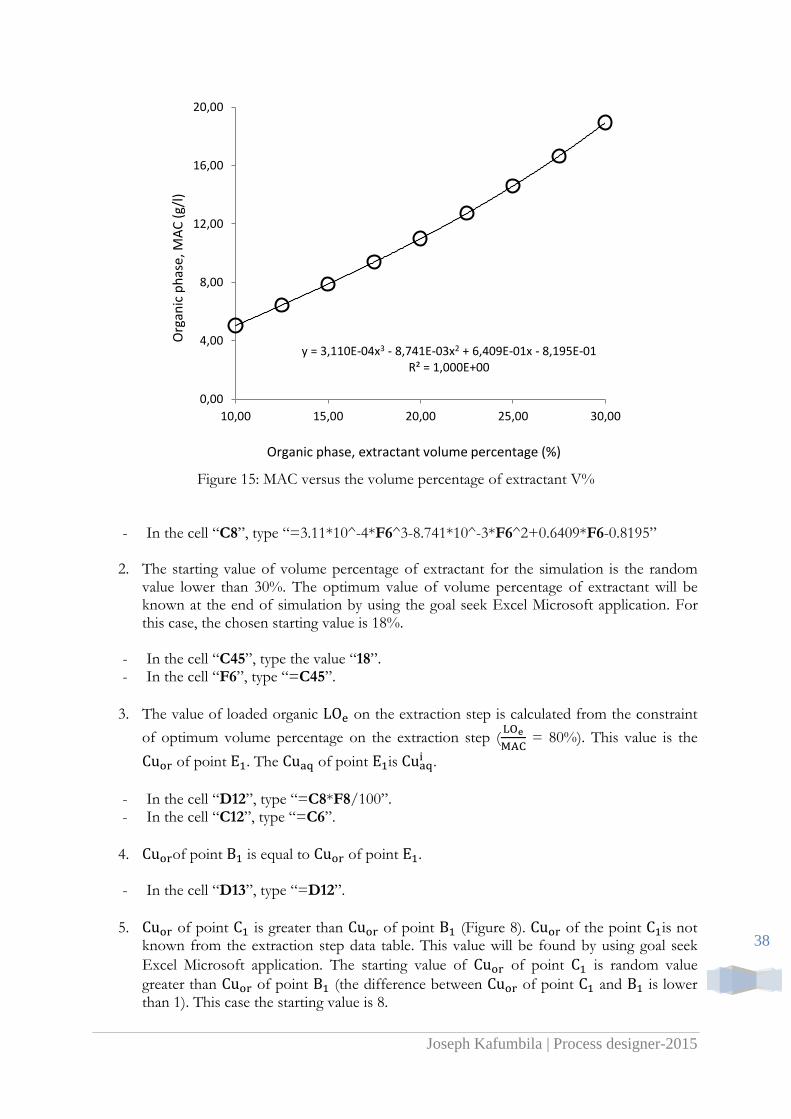
1. The simulation is started by the calculation of MAC value for the PLS at different value of volume percentage of extractant in the organic phase. If the extraction step is made by more than one cascades (series – parallel, interlaced, and others), the MAC value is calculated with the first PLS which is the feed of stage of rank “1” on the extraction step. The results of MAC value are in Table 17 and Figure 15. From Figure 15, the extrapolation curve which gives the value of MAC versus the volume percentage of extractant is found from Excel Microsoft application. The mathematical expression of extrapolation curve is given on Figure 15. Table 17: MAC value for different value of volume percentage of extractant
V%
- MAC
% g/l g/l g/l
10.0 7 4 2.286 2.286 0.00 5.04
12.5 7 4 2.286 2.286 0.00 6.42
15.0 7 4 2.286 2.286 0.00 7.87
17.5 7 4 2.286 2.286 0.00 9.39
20.0 7 4 2.286 2.286 0.00 11.00
22.5 7 4 2.286 2.286 0.00 12.73
25.0 7 4 2.286 2.286 0.00 14.59
27.5 7 4 2.286 2.286 0.00 16.65
30.0 7 4 2.286 2.286 0.00 18.95
E1 E2
S1 S2
PLS Raf
SOe LOe
SOs LOs
AD SP
Joseph Kafumbila | Process designer-2015
38
Figure 15: MAC versus the volume percentage of extractant V%
- In the cell “C8”, type “=3.11*10^-4*F6^3-8.741*10^-3*F6^2+0.6409*F6-0.8195”
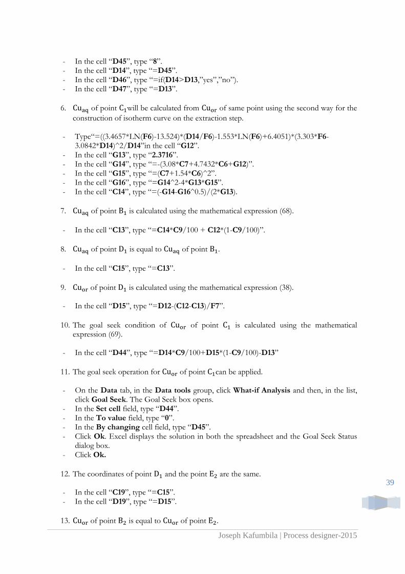
2. The starting value of volume percentage of extractant for the simulation is the random value lower than 30%. The optimum value of volume percentage of extractant will be known at the end of simulation by using the goal seek Excel Microsoft application. For this case, the chosen starting value is 18%.
- In the cell “C45”, type the value “18”. - In the cell “F6”, type “=C45”.
3. The value of loaded organic on the extraction step is calculated from the constraint
of optimum volume percentage on the extraction step (
= 80%). This value is the
of point . The of point is .
- In the cell “D12”, type “=C8*F8/100”. - In the cell “C12”, type “=C6”.
4. of point is equal to of point .
- In the cell “D13”, type “=D12”.
5. of point is greater than of point (Figure 8). of the point is not known from the extraction step data table. This value will be found by using goal seek
Excel Microsoft application. The starting value of of point is random value
greater than of point (the difference between of point and is lower than 1). This case the starting value is 8.
y = 3,110E-04x3 - 8,741E-03x2 + 6,409E-01x - 8,195E-01 R² = 1,000E+00
0,00
4,00
8,00
12,00
16,00
20,00
10,00 15,00 20,00 25,00 30,00
Org
anic
ph
ase,
MA
C (
g/l)
Organic phase, extractant volume percentage (%)
Joseph Kafumbila | Process designer-2015
39
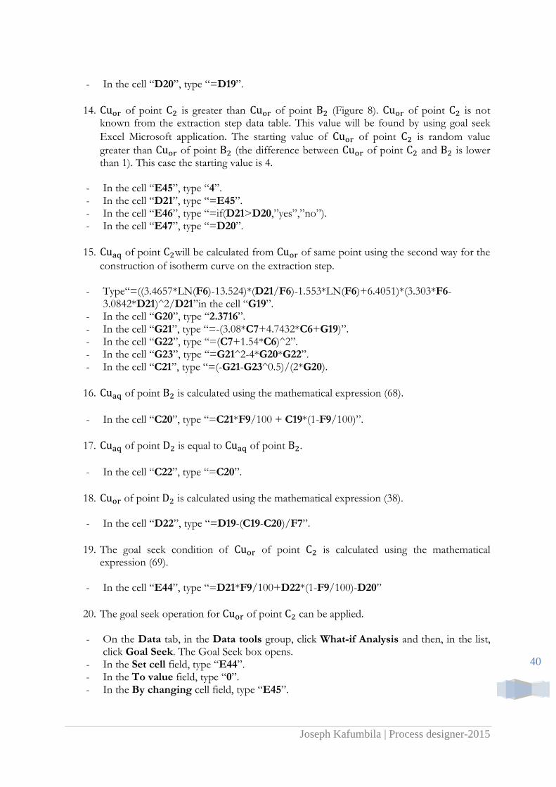
- In the cell “D45”, type “8”. - In the cell “D14”, type “=D45”. - In the cell “D46”, type “=if(D14>D13,”yes”,”no”). - In the cell “D47”, type “=D13”.
6. of point will be calculated from of same point using the second way for the
construction of isotherm curve on the extraction step.
- Type“=((3.4657*LN(F6)-13.524)*(D14/F6)-1.553*LN(F6)+6.4051)*(3.303*F6-3.0842*D14)^2/D14”in the cell “G12”.
- In the cell “G13”, type “2.3716”. - In the cell “G14”, type “=-(3.08*C7+4.7432*C6+G12)”. - In the cell “G15”, type “=(C7+1.54*C6)^2”. - In the cell “G16”, type “=G14^2-4*G13*G15”. - In the cell “C14”, type “=(-G14-G16^0.5)/(2*G13).
7. of point is calculated using the mathematical expression (68).
- In the cell “C13”, type “=C14*C9/100 + C12*(1-C9/100)”.
8. of point is equal to of point .
- In the cell “C15”, type “=C13”.
9. of point is calculated using the mathematical expression (38).
- In the cell “D15”, type “=D12-(C12-C13)/F7”.
10. The goal seek condition of of point is calculated using the mathematical expression (69).
- In the cell “D44”, type “=D14*C9/100+D15*(1-C9/100)-D13”
11. The goal seek operation for of point can be applied.
- On the Data tab, in the Data tools group, click What-if Analysis and then, in the list, click Goal Seek. The Goal Seek box opens.
- In the Set cell field, type “D44”. - In the To value field, type “0”. - In the By changing cell field, type “D45”. - Click Ok. Excel displays the solution in both the spreadsheet and the Goal Seek Status
dialog box. - Click Ok.
12. The coordinates of point and the point are the same.
- In the cell “C19”, type “=C15”. - In the cell “D19”, type “=D15”.
13. of point is equal to of point .
Joseph Kafumbila | Process designer-2015
40
- In the cell “D20”, type “=D19”.
14. of point is greater than of point (Figure 8). of point is not known from the extraction step data table. This value will be found by using goal seek
Excel Microsoft application. The starting value of of point is random value
greater than of point (the difference between of point and is lower than 1). This case the starting value is 4.
- In the cell “E45”, type “4”. - In the cell “D21”, type “=E45”. - In the cell “E46”, type “=if(D21>D20,”yes”,”no”). - In the cell “E47”, type “=D20”.
15. of point will be calculated from of same point using the second way for the
construction of isotherm curve on the extraction step.
- Type“=((3.4657*LN(F6)-13.524)*(D21/F6)-1.553*LN(F6)+6.4051)*(3.303*F6-3.0842*D21)^2/D21”in the cell “G19”.
- In the cell “G20”, type “2.3716”. - In the cell “G21”, type “=-(3.08*C7+4.7432*C6+G19)”. - In the cell “G22”, type “=(C7+1.54*C6)^2”. - In the cell “G23”, type “=G21^2-4*G20*G22”. - In the cell “C21”, type “=(-G21-G23^0.5)/(2*G20).
16. of point is calculated using the mathematical expression (68).
- In the cell “C20”, type “=C21*F9/100 + C19*(1-F9/100)”.
17. of point is equal to of point .
- In the cell “C22”, type “=C20”.
18. of point is calculated using the mathematical expression (38).
- In the cell “D22”, type “=D19-(C19-C20)/F7”.
19. The goal seek condition of of point is calculated using the mathematical expression (69).
- In the cell “E44”, type “=D21*F9/100+D22*(1-F9/100)-D20”
20. The goal seek operation for of point can be applied.
- On the Data tab, in the Data tools group, click What-if Analysis and then, in the list, click Goal Seek. The Goal Seek box opens.
- In the Set cell field, type “E44”. - In the To value field, type “0”. - In the By changing cell field, type “E45”.
Joseph Kafumbila | Process designer-2015
41
- Click Ok. Excel displays the solution in both the spreadsheet and the Goal Seek Status dialog box.
- Click Ok.
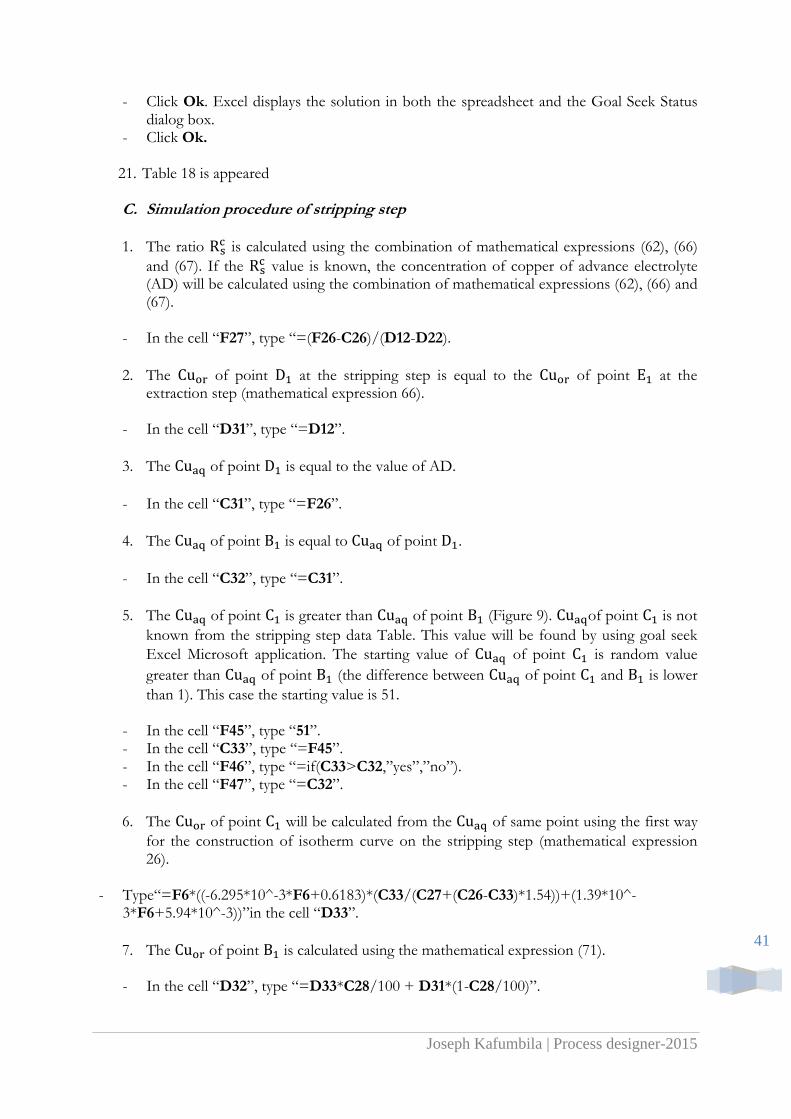
21. Table 18 is appeared
C. Simulation procedure of stripping step
1. The ratio is calculated using the combination of mathematical expressions (62), (66)
and (67). If the value is known, the concentration of copper of advance electrolyte
(AD) will be calculated using the combination of mathematical expressions (62), (66) and (67).
- In the cell “F27”, type “=(F26-C26)/(D12-D22).
2. The of point at the stripping step is equal to the of point at the extraction step (mathematical expression 66).
- In the cell “D31”, type “=D12”.
3. The of point is equal to the value of AD.
- In the cell “C31”, type “=F26”.
4. The of point is equal to of point .
- In the cell “C32”, type “=C31”.
5. The of point is greater than of point (Figure 9). of point is not
known from the stripping step data Table. This value will be found by using goal seek
Excel Microsoft application. The starting value of of point is random value
greater than of point (the difference between of point and is lower
than 1). This case the starting value is 51.
- In the cell “F45”, type “51”. - In the cell “C33”, type “=F45”. - In the cell “F46”, type “=if(C33>C32,”yes”,”no”). - In the cell “F47”, type “=C32”.
6. The of point will be calculated from the of same point using the first way
for the construction of isotherm curve on the stripping step (mathematical expression 26).
- Type“=F6*((-6.295*10^-3*F6+0.6183)*(C33/(C27+(C26-C33)*1.54))+(1.39*10^-3*F6+5.94*10^-3))”in the cell “D33”.
7. The of point is calculated using the mathematical expression (71).
- In the cell “D32”, type “=D33*C28/100 + D31*(1-C28/100)”.
Joseph Kafumbila | Process designer-2015
42
A B C D E F G H
1
2 Table 18: simulation table of copper solvent extraction
3
4 Extraction step
5 Extraction step data
6 7 g/l 18 %
7 4 g/l
1.1
8 MAC 9.698 g/l LO/MAC 80 %
9 93 % 95 %
10
11 Stage 1 Parameters
12 7 7.759 51.728
13 2.708 7.759 A 2.3716
14 2.385 8.052 B -97.250
15 2.708 3.857 C 218.45
16 Δ 7.385E+03
17
18 Stage 2 Parameters
19 2.708 3.857 643.21
20 0.437 3.857 A 2.3716
21 0.318 3.966 B -688.73
22 0.437 1.792 C 218.45
23 Δ 4.723E+05
24 Stripping step
25 Stripping step Data
26 35 g/l AD 50 g/l
27 180 g/l
28 98 % 98 %
29
30 Stage 1
31
32
33
34
35
36 Stage 2
37
38
39
40
41
42 Goal seek
43 1 2 3 4 5
44 Set cell 0.000 0.000
45 By changing 18 8.052 3.966
46 Conditions Yes Yes
47 B value 7.759 3.857
48
Joseph Kafumbila | Process designer-2015
43
8. The of point is equal to the of point .
- In the cell “D34”, type “=D32”.
9. The of point is calculated using the mathematical expression (54).
- In the cell “C34”, type “=C31-F27*(D31-D34)”.
10. The goal seek condition of of point is calculated using the mathematical
expression (70).
- In the cell “F44”, type “=C33*C28/100+C34*(1-C28/100)-C32”
11. The goal seek operation for of point can be applied.
- On the Data tab, in the Data tools group, click What-if Analysis and then, in the list,
click Goal Seek. The Goal Seek box opens. - In the Set cell field, type “F44”. - In the To value field, type “0”. - In the By changing cell field, type “F45”. - Click Ok. Excel displays the solution in both the spreadsheet and the Goal Seek Status
dialog box. - Click Ok.
12. The coordinates of point and the point are the same.
- In the cell “C37”, type “=C34”. - In the cell “D37”, type “=D34”.
13. The of point is equal to of point .
- In the cell “C38”, type “=C37”.
14. The of point is greater than of point (Figure 9). of point is
not known from the stripping step data Table. This value will be found by using goal
seek Excel Microsoft application. The starting value of of point is random value
greater than of point (the difference between of point and is lower
than 1). This case the starting value is 40.
- In the cell “G45”, type “40”. - In the cell “C39”, type “=G45”. - In the cell “G46”, type “=if(C39>C38,”yes”,”no”). - In the cell “G47”, type “=C38”.
15. The of point will be calculated from the of same point using the first way
for the construction of isotherm curve on the stripping step (mathematical expression 26).
- Type“=F6*((-6.295*10^-3*F6+0.6183)*(C39/(C27+(C26-C39)*1.54))+(1.39*10^-3*F6+5.94*10^-3))”in the cell “D39”.
Joseph Kafumbila | Process designer-2015
44
16. The of point is calculated using the mathematical expression (71).
- In the cell “D38”, type “=D39*F28/100 + D37*(1-F28/100)”.
17. The of point is equal to the of point .
- In the cell “D40”, type “=D38”.
18. The of point is calculated using the mathematical expression (54).
- In the cell “C40”, type “=C37-F27*(D37-D40)”.
19. The goal seek condition of of point is calculated using the mathematical
expression (70).
- In the cell “G44”, type “=C39*F28/100+C40*(1-F28/100)-C38”
20. The goal seek operation for of point can be applied.
- On the Data tab, in the Data tools group, click What-if Analysis and then, in the list,
click Goal Seek. The Goal Seek box opens. - In the Set cell field, type “G44”. - In the To value field, type “0”. - In the By changing cell field, type “G45”. - Click Ok. Excel displays the solution in both the spreadsheet and the Goal Seek Status
dialog box. - Click Ok.
D. Goal seek operation of volume percentage of extractant
1. The goal seek condition of volume percentage of extractant is calculated using the
mathematical expression (67).
- In the cell “C44”, type “=D22-D40”
2. It appears Table 19.
3. The goal seek operation for V% can be applied.
- On the Data tab, in the Data tools group, click What-if Analysis and then, in the list, click Goal Seek. The Goal Seek box opens.
- In the Set cell field, type “C44”. - In the To value field, type “0”. - In the By changing cell field, type “C45”. - Click Ok. Excel displays the solution in both the spreadsheet and the Goal Seek Status
dialog box. - Click Ok.

Joseph Kafumbila | Process designer-2015
45
A B C D E F G H
1
2 Table 19: simulation table of copper solvent extraction
3
4 Extraction step
5 Extraction step data
6 7 g/l 18 %
7 4 g/l
1.1
8 MAC 9.698 g/l LO/MAC 80 %
9 93 % 95 %
10
11 Stage 1 Parameters
12 7 7.759 51.728
13 2.708 7.759 A 2.3716
14 2.385 8.052 B -97.250
15 2.708 3.857 C 218.45
16 Δ 7.385E+03
17
18 Stage 2 Parameters
19 2.708 3.857 643.21
20 0.437 3.857 A 2.3716
21 0.318 3.966 B -688.73
22 0.437 1.792 C 218.45
23 Δ 4.723E+05
24 Stripping step
25 Stripping step Data
26 35 g/l AD 50 g/l
27 180 g/l
2.514
28 98 % 98 %
29
30 Stage 1
31 50.00 7.759
32 50.00 3.558
33 50.22 3.473
34 39.44 3.558
35
36 Stage 2
37 39.44 3.558
38 39.44 2.649
39 39.49 2.631
40 37.15 2.649
41
42 Goal seek
43 1 2 3 4 5
44 Set cell 0.000 0.000 0.000 0.000
45 By changing 18 8.052 3.966 50.22 39.49
46 Conditions Yes Yes Yes Yes
47 B value 7.759 3.857 50.00 39.44
48
Joseph Kafumbila | Process designer-2015
46
A B C D E F G H
1
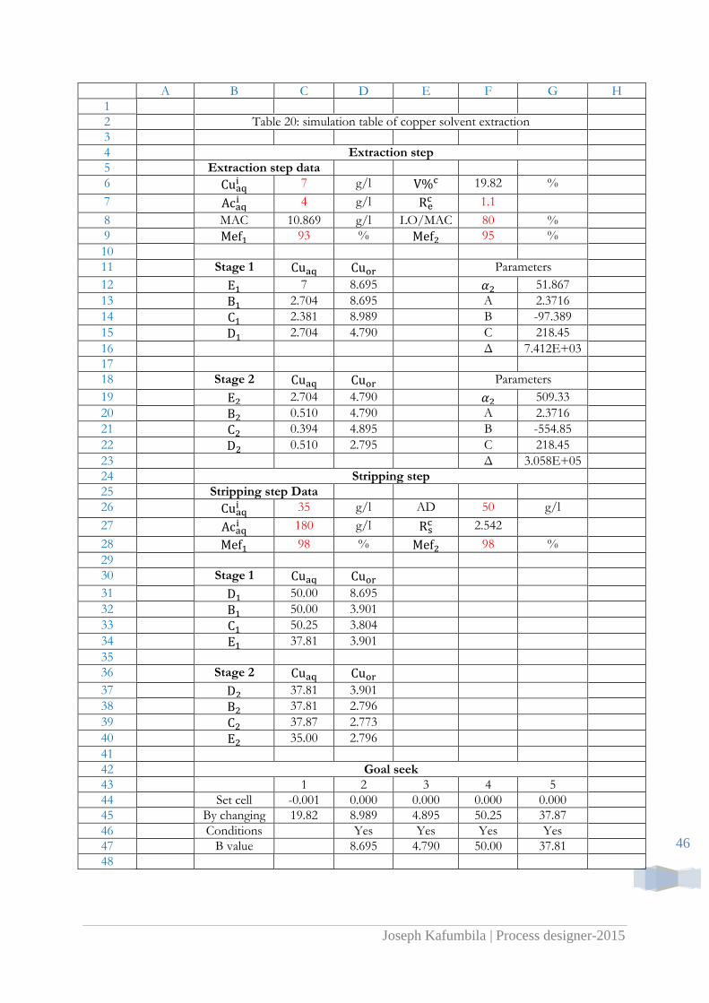
2 Table 20: simulation table of copper solvent extraction
3
4 Extraction step
5 Extraction step data
6 7 g/l 19.82 %
7 4 g/l
1.1
8 MAC 10.869 g/l LO/MAC 80 %
9 93 % 95 %
10
11 Stage 1 Parameters
12 7 8.695 51.867
13 2.704 8.695 A 2.3716
14 2.381 8.989 B -97.389
15 2.704 4.790 C 218.45
16 Δ 7.412E+03
17
18 Stage 2 Parameters
19 2.704 4.790 509.33
20 0.510 4.790 A 2.3716
21 0.394 4.895 B -554.85
22 0.510 2.795 C 218.45
23 Δ 3.058E+05
24 Stripping step
25 Stripping step Data
26 35 g/l AD 50 g/l
27 180 g/l
2.542
28 98 % 98 %
29
30 Stage 1
31 50.00 8.695
32 50.00 3.901
33 50.25 3.804
34 37.81 3.901
35
36 Stage 2
37 37.81 3.901
38 37.81 2.796
39 37.87 2.773
40 35.00 2.796
41
42 Goal seek
43 1 2 3 4 5
44 Set cell -0.001 0.000 0.000 0.000 0.000
45 By changing 19.82 8.989 4.895 50.25 37.87
46 Conditions Yes Yes Yes Yes
47 B value 8.695 4.790 50.00 37.81
48
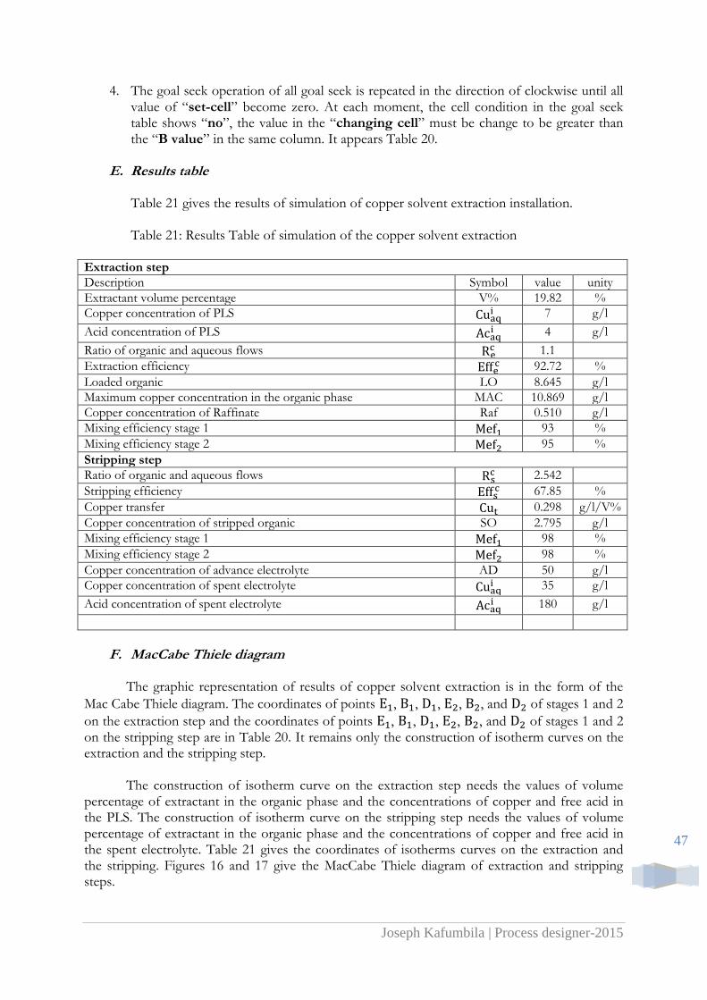
Joseph Kafumbila | Process designer-2015
47
4. The goal seek operation of all goal seek is repeated in the direction of clockwise until all value of “set-cell” become zero. At each moment, the cell condition in the goal seek table shows “no”, the value in the “changing cell” must be change to be greater than the “B value” in the same column. It appears Table 20.
E. Results table Table 21 gives the results of simulation of copper solvent extraction installation. Table 21: Results Table of simulation of the copper solvent extraction
Extraction step
Description Symbol value unity
Extractant volume percentage V% 19.82 %
Copper concentration of PLS 7 g/l
Acid concentration of PLS 4 g/l
Ratio of organic and aqueous flows 1.1
Extraction efficiency 92.72 %
Loaded organic LO 8.645 g/l
Maximum copper concentration in the organic phase MAC 10.869 g/l
Copper concentration of Raffinate Raf 0.510 g/l
Mixing efficiency stage 1 93 %
Mixing efficiency stage 2 95 %
Stripping step
Ratio of organic and aqueous flows 2.542
Stripping efficiency 67.85 %
Copper transfer 0.298 g/l/V%
Copper concentration of stripped organic SO 2.795 g/l
Mixing efficiency stage 1 98 %
Mixing efficiency stage 2 98 %
Copper concentration of advance electrolyte AD 50 g/l
Copper concentration of spent electrolyte 35 g/l
Acid concentration of spent electrolyte 180 g/l
F. MacCabe Thiele diagram
The graphic representation of results of copper solvent extraction is in the form of the
Mac Cabe Thiele diagram. The coordinates of points , , , , , and of stages 1 and 2
on the extraction step and the coordinates of points , , , , , and of stages 1 and 2 on the stripping step are in Table 20. It remains only the construction of isotherm curves on the extraction and the stripping step.
The construction of isotherm curve on the extraction step needs the values of volume
percentage of extractant in the organic phase and the concentrations of copper and free acid in the PLS. The construction of isotherm curve on the stripping step needs the values of volume percentage of extractant in the organic phase and the concentrations of copper and free acid in the spent electrolyte. Table 21 gives the coordinates of isotherms curves on the extraction and the stripping. Figures 16 and 17 give the MacCabe Thiele diagram of extraction and stripping steps.
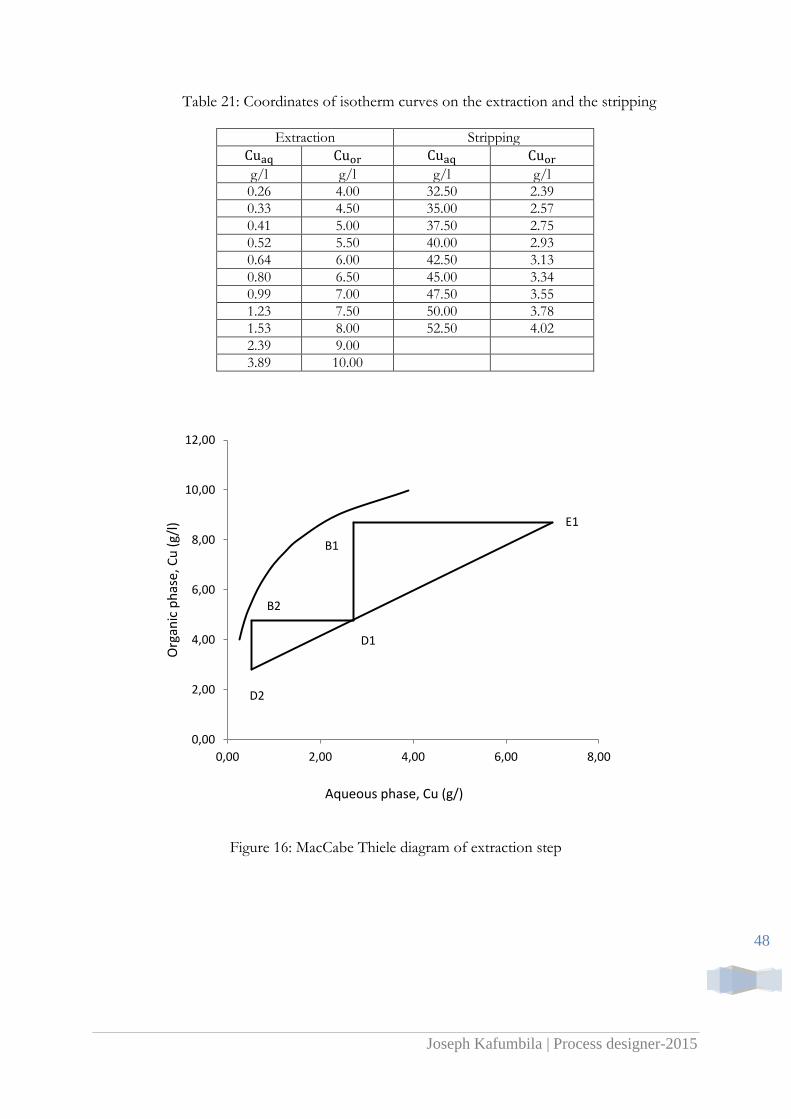
Joseph Kafumbila | Process designer-2015
48
Table 21: Coordinates of isotherm curves on the extraction and the stripping
Extraction Stripping
g/l g/l g/l g/l
0.26 4.00 32.50 2.39
0.33 4.50 35.00 2.57
0.41 5.00 37.50 2.75
0.52 5.50 40.00 2.93
0.64 6.00 42.50 3.13
0.80 6.50 45.00 3.34
0.99 7.00 47.50 3.55
1.23 7.50 50.00 3.78
1.53 8.00 52.50 4.02
2.39 9.00
3.89 10.00
Figure 16: MacCabe Thiele diagram of extraction step
E1
B1
D1
B2
D2
0,00
2,00
4,00
6,00
8,00
10,00
12,00
0,00 2,00 4,00 6,00 8,00
Org
anic
ph
ase,
Cu
(g/
l)
Aqueous phase, Cu (g/)

Joseph Kafumbila | Process designer-2015
49
Figure 17: MacCabe Thiele diagram of stripping step
D1
B1 E1
B2 E2
0,00
2,00
4,00
6,00
8,00
10,00
30,00 35,00 40,00 45,00 50,00 55,00
Org
anic
ph
ase
, Cu
(g/
l)
Aqueous phase, Cu (g/l)
Joseph Kafumbila | Process designer-2015
50
References
1. Hossen Aminian, Modélisation et simulation des opérations d’extraction par solvant et d’électrolyse du Cuivre, thèse, université de Laval, Canada, 1999.
2. Gerald L. Bauer and Thomas W. Chapman, Measurement and correlation of solvent extraction equilibria. The extraction of Copper by kelex 100, Metallurgical transaction B, 1976.
3. AMEL A., Etude thermodynamique de l’extraction des Métaux de transition par la
Salicylidèneaniline, thèse, Université Mohamed Khider, 2013.
4. BASF, Redbook mining solutions, 2014.
5. Sorderstrom M., Bednarki T., Villegas E., Stage efficiency in Copper solvent extraction Plants, technical paper, 2010.
6. Cognis, Copper solvent extraction training, 2007.
7. Murdoch Mackenzie, The solvent extraction of some major metals: overviews, Henkel
Australia Pty ltd.
8. Jeffers T.H, Groves R.D, Minimizing lead contamination in copper produced by solvent extraction – electrowinning, Salt Lake City Research Center.
9. Cl. Feneau, R. Breckpot, Problèmes relatifs à l’électrocristallisation du cuivre, Laboratoire
de chimie minérale, université de Louvain.
10. Liu Jiarshe, Lan Zhuo Yue, Qiu Guarr Zhou, Wang Diarr Zuo, Mechanism of crud formation in copper solvent extraction, journal CSUT, Vol 9, 2002.
11. Hans Hein, Importance of a wash stage in copper solvent extraction, Hydrocopper, 2005.