Embed Size (px)
Citation preview

1
DET TEKNISK-NATURVITENSKAPELIGE FAKULTET
MASTEROPPGAVE
Studieprogram/spesialisering:
Petroleum
Vår.................semesteret, 2009....
Åpen / Konfidensiell
Forfatter:
Signe Husebø
…………………………………………
(signatur forfatter)
Faglig ansvarlig Erik Skaugen
Veileder(e): Pål Hjertholm
Tittel på masteroppgaven:
Engelsk tittel:
Real Time Production Monitoring with Prediction and Validation
Studiepoeng:

2
Emneord:
WellFlo
ReO
Monitoring
Validation
Real-time production
Verification
Sidetall: …………………
+ vedlegg/annet: …………
Stavanger, ………………..
dato/år
3
Content Acknowledgement ................................................................................................................................... 6
Abstract ................................................................................................................................................... 7
1. Introduction ..................................................................................................................................... 8
1.1 Background .............................................................................................................................. 8
1.2 Optimization Potential ............................................................................................................ 8
1.2.1 Transmitters .................................................................................................................... 8
2 Theory .............................................................................................................................................. 9
2.1 Inflow and Outflow Theory ..................................................................................................... 9
2.1.1 IPR and TPR curves .......................................................................................................... 9
2.1.2 Vogel Inflow Performance ............................................................................................... 9
2.2 Scale ....................................................................................................................................... 10
2.2.1 Scale deposition in the choke valve. ............................................................................. 10
2.3 Allocation ............................................................................................................................... 10
2.3.1 Well tests ....................................................................................................................... 10
2.3.2 Well test practice:.......................................................................................................... 11
2.4 Real Time Data....................................................................................................................... 11
2.4.1 Optimum Online ............................................................................................................ 11
2.4.2 PI Systems ...................................................................................................................... 11
2.5 Models .................................................................................................................................. 12
2.5.1 WellFlo ........................................................................................................................... 12
2.5.2 ReO ................................................................................................................................ 12
2.5.3 The Network Model ....................................................................................................... 12
2.5.4 The Chokes at Ekofisk ........................................................................................................... 13
2.6 Multiphase flow ..................................................................................................................... 13
2.6.1 Pressure drop. ............................................................................................................... 13
2.6.2 Pressure Gradient Correlations drop between the bottomhole and the wellhead. ..... 14
2.6.3 Flow regimes. ................................................................................................................ 14
2.6.4 Multiphase Flow through Chokes .................................................................................. 15
2.6.5 Critical and Subcritical Flow........................................................................................... 15
2.7 Flow velocities ....................................................................................................................... 16
2.7.1 Superficial Velocities ..................................................................................................... 16
2.7.2 Phase Velocities ............................................................................................................. 17
4
2.7.3 Relative phase velocities and slip .................................................................................. 17
2.7.4 Fluid Fractions ............................................................................................................... 17
2.7.5 Fractions at slip .............................................................................................................. 18
2.7.6 Density ........................................................................................................................... 18
2.8 In-situ conditions ................................................................................................................... 18
2.8.1 Compressibility factor.................................................................................................... 18
2.8.2 Critical state ................................................................................................................... 18
2.8.3 Critical Temperature and Pressure ................................................................................ 19
2.9 Bernoulli – One phase ........................................................................................................... 19
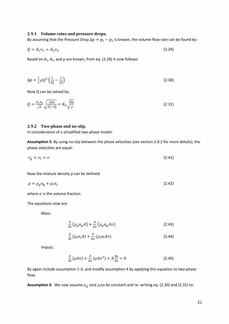
2.9.1 Volume rates and pressure drops. ................................................................................ 21
2.9.2 Two-phase and no-slip. ................................................................................................. 21
2.9.3 Bernoulli expressed by Pressure Drop. ......................................................................... 22
2.9.4 Free slip ......................................................................................................................... 22
2.9.5 Volume rates expressed by the Pressure Drop. ............................................................ 23
3 Calculations and Analysis in WellFlo ............................................................................................. 24
3.1 Tuning Procedure in Wellflo .................................................................................................. 24
3.1.1 Well parameters ............................................................................................................ 24
3.1.2 Input parameters ........................................................................................................... 25
3.2 Pressure drop correlations .................................................................................................... 25
3.2.1 Tuning with L-factor ...................................................................................................... 26
3.2.2 Temperature gradient Correlations in WellFlo ............................................................. 26
3.2.3 Oil-Water slippage in WellFlo ........................................................................................ 31
3.2.4 Surface Choke ................................................................................................................ 31
3.2.5 WellFlo reports .............................................................................................................. 31
4 The Analysis ................................................................................................................................... 33
4.1 Objective of the study ........................................................................................................... 33
4.2 The procedure ....................................................................................................................... 33
4.2.1 The Pressure Ratio ......................................................................................................... 33
4.2.2 A Temperature Verification ........................................................................................... 33
4.2.3 Pressure Drop Measurements Across Choke ............................................................... 34
4.2.4 Discharge Coefficient ..................................................................................................... 35
4.2.5 Building the flow rate model ......................................................................................... 37
4.2.6 The mixture density ....................................................................................................... 38
4.3 Dummy tests.......................................................................................................................... 38
5 Results and discussion ................................................................................................................... 40
5
6 Conclusion and Recommendations ............................................................................................... 44
References ............................................................................................................................................. 45
Nomenclature ........................................................................................................................................ 46
Appendix A ............................................................................................................................................ 48
Appendix B ............................................................................................................................................ 76
6
Acknowledgement
This thesis was done for the University of Stavanger at the department of Petroleum Institute. I
would like to thank my supervisor professor Erik Skaugen for his engagement and support in my
work.
The work was performed at Optimum Production and I am pleased to have had the opportunity to
write my thesis for the company and use their data and program license in my studies. I want to give
my special thanks to the Managing Director Pål Hjertholm, for shearing his innovative ideas and
motivations. I would also like to thank Erik Haug and Ottar Salvigsen for their guidance and teaching.
I also would like to thank my good friend and cousin, professor Tore Halsne Flåtten at NTNU, for the
constructive conversations and his shearing e-mail correspondence.
7
Abstract
This Master of Science studies Optimum Online’s real time estimated production at the Ekofisk Field.
Information from offshore process sensors are used to validate the individual well estimates and to
detect any deviation in a wells performance.
In order to ensure the quality of the estimated production, a temperature verification is used by
monitoring the differences between the calculated temperature in the simulations and the measured
temperature at the wellhead. An accepted limit in deviations determines if the production is verified
or not. Solutions for improvement of estimates during an unverified period are suggested, depending
on what cause the change in well behaviour.
Upstream and downstream choke pressures, and choke size are used to predict a flowrate through
choke. The flowrate is compared to Optimum Online real-time estimates and to welltests. The aim is
to find an expression of a predicted flow rate that is a function of the pressure drop and may detect a
decline in production. The flowrate will be thoroughly examined before implemented and tested in
Optimum off line version and checked for verification.
8
1. Introduction
1.1 Background The Ekofisk and Eldfisk fields are one of the largest and most important fields in the North Sea. Both
fields are producing from chalk reservoirs located within the PLO018 license area. As of January 2009
a daily production of 213,000 bbl/d are produced from 104 wells and furthermore 34 wells are water
injectors. 41 of the producers are on gas lift.
1.2 Optimization Potential Integrated operations (IO) and production optimisation are highly focused in the petroleum industry
worldwide. One of the key elements in production optimisation is teamwork based on real time data,
monitoring, allocating, implementation and development. Extended use of real time data is essential
for the future production optimisation and the industry is focused on integrating real time data into
the work processes, turning the high frequency data into real value to be able of early detection of
unwanted well performance, better and more frequently decision making in order to optimize
production, simpler workflows and rationalised planning.
One important advance in the oil industry operations is monitoring the process by using real time
data. This allows doing faster diagnostic, and faster and more effective decisions.
Determining the individual well rates is an important task in the measurements of total produced oil
and gas. The basis of determination of a wells contribution is well testing, and is still the leading
principle in determining the individual well flow rates today. Integrated operations enables allocation
in real-time and contributes to continuous well monitoring and individual wells performance.
1.2.1 Transmitters
Huge amounts of data are generated from sensors in a production system of wells. The sensors are
placed at wellhead, upstream choke, downstream choke, downhole gauges, separators and at the
flow lines. Downhole gauge is placed at the fluid column in the well, and the pressure and
temperature are used for trend analysis, and simulation correlations which can be implemented in
well analysis.
A field model which is continuously updated can help the engineers optimise, forecast and track
developing trends in production. As with all models, high quality input data is needed to get quality
output.

9
2 Theory
2.1 Inflow and Outflow Theory The operating conditions in a well can change during the traditional allocation period of one month
before updating, as the reservoir parameters (Pres,WC, GOR) changes during depletion. This may lead
to incorrectly allocated values for the well production.
2.1.1 IPR and TPR curves
The well head pressure is proportional to the bottomhole pressure at a constant rate. A decrease in
the downhole pressure could be a consequence of natural depletion in the reservoir, skin or a scale
bridge. This will imply a reduced wellhead pressure. The behaviour of the temperature is more
complex such as change in heat transfer along the pipe due to change in flow rate. However there
are methods in simulation programs with correlations and analyses with their respectively
calculations.
IPR curves are made from two parameters, drawdown also called productivity index (PI), and the
reservoir pressure. PI is the slope of the IPR curve, while Pres is the point where the curve crosses the
y-axis and the flowrate equals zero. [4] The TPR curve is affected by tubing parameters as pipe size,
wall roughness, wellhead pressure and gas lift rate.
2.1.2 Vogel Inflow Performance
The Vogel relation [7] is used for calculating the Inflow performance in wells. The inflow performance
curve model is used in this study. The inflow is given by:
(2.1)
where
qo - is the oil rate,
qo max -is the max oil rate when Pwf=0,
Pwf -is the wellbore flowing pressure, and
Pr - is the reservoir pressure
A vertical lift performance curve indicates what a well is expected to produce at a given wellhead
pressure and is traditionally updated using well test results. The sum of these theoretical well rates
should ideally match the measured total production. Deviations are determined from the allocation
factor, hence giving an idea of the uncertainty in the estimated production.
The inflow performance (IPR) and vertical lift performance (VLP) is combined to provide the well
deliverability. The intersection of the plots of flow rate versus the bottomhole pressure of these two
components gives the expected deliverability. The intersection also describes a specific instant of the
well and depends strongly on the type of flow regime controlling the well performance.

10
2.2 Scale After water breakthrough the produced flow rate will contain water. This can be confirmed by
increasing watercut. An analysis of the produced water will determine if it is the formation water or
injected water that is present in the reservoir.
Formation of scale is mainly due to the mixing of the formation water and the sea water injected into
the reservoir. The formation water contains ions of Barium and Strontium, while the seawater
contributes with ions of sulphate. When the combination of right temperature and pressure are
present the ions may react with the chalk and form scale.
Scale can be present in the perforations, in the tubing or at the surface facilities, such as the choke or
in the flow line. A scale problem may lead to production loss and is an increasingly problem at the
Ekofisk field due to the increase in produced water.
2.2.1 Scale deposition in the choke valve.
The most common location of scale deposition in the flow line is where a pressure drop may occur or
the flow passes through a restriction. Therefore, a choke valve is sensitive to scale deposition since
part of the valve consists of several smaller holes exposed to the flow, depending on the choke
setting. These holes may slowly plug up from scale and will also over time affect the actual choke
size.
2.3 Allocation “the mathematical process of assigning portions of a commingled production stream to the sources,
typically wells, leases, units, or production facilities, which contributed to the total flow through a
custody transfer or allocation measurement point.” *1+
Total produced volume in a field is the sum of individual production from all contributing wells. The
total production is measured as total oil, water and gas phase at separator and measured as single
phases afterwards and is hence regarded to be of sufficient accuracy. Describing the multiphase
individual well stream is more complex as the constituents vary in their physical properties as
density, viscosity and chemical composition. The common way to find the single well rates is by well
testing with a test separator. In order tp redistribute the total measured production rate back to the
individual wells, good allocation routines are required.
2.3.1 Well tests
The most common form of well testing are the single rate drawdown test, the pressure build up test,
and the multi-rate drawdown test. The production is routed to a test separator to perform analysis
and measurements. Each well is tested approximately once a month, depending on well stability and
performance.

11
Well testing is mainly required to allocate the production of hydrocarbons to each well and to update
the reservoir parameters in the models. It is also used to monitor well performance.
2.3.2 Well test practice:
Well flow lines are routed to the test separator and the output flows of oil, gas and water are
measured after some hours when the flow is believed to be reasonably stable. A welltest usually
takes four hours and the flowrate is averaged during the test periode.
2.4 Real Time Data
2.4.1 Optimum Online
Optimum Online retrieve and treats data from different sources and represents the results in a web
interface. The Online system provides production simulation by process real-time values from
offshore platforms to an onshore network system. The network system is a field model witch takes
into account all the limitations in a production process. A well model for each single well in the field
is implemented in the network system. The well model will be updated and tuned by new welltests.
Each single well and is thereby monitoring any deviation from the production forecast. Different
equipment or operation parameters can be changed in the models to analyze a production
optimization or to prevent undesirable influence on the production system. Figure 2.1 is showing the
information process.
The main data source in Optimum Online is the PI System data base. Welltest results are retrieved
from NPAS .
Figure 2.1. is showing how the information is collected in a simulation.
2.4.2 PI Systems
PI systems receive all types of data from the control systems, transmitters and simulation results and
represents data in a web interface. Measurements from transmitters are automatic transferred via
fiber optic cable to PI database. The information can be loaded and visualized graphically with
current and historic data. Another option is to load datasets direct to excel and do further analysis. In
this work, excel is primarily used for loading data from transmitters, but also to do statistic analysis,
Welltest
Welltest
Wellmodel
tuned
Network
modell
(88888888
88888888(
ReO)
Optimum
Online
PI Database
P,T,
Choke,ga
Estimated
production

12
such as calculating the average and mean values for a certain period. Optimum Online load real-time
data from PI database.
2.5 Models Two types of software modelling programs are used in the context of this work, WellFlo which is a
well model program, and ReO which is a field model program. The well model incorporates
multiphase flow from near well bore via the point it enters a well bore and until it reaches the
wellhead. There is one well model for each well, with the PVT parameters, equipment geometry,
artificial lift, geothermal gradient and heat capacity controlling the output. The field model consists
of all well models in a field connected to the topside facilities to model the comingled flows.
2.5.1 WellFlo
WellFlo is an application for a single well performance analysis where well test data are being
analysed. The software includes building the well with relevant completion, depth, inclination and
dimensions in the tube. Fluid parameters are PVT data, viscosity, densities, API and flow type. Input
parameters are GOR, water cut, flow rates, temperatures and pressure during the well test. Based on
reservoir parameters the IPR and VLP curves will be constructed and used to calculate an operating
point. Several tube correlations are available matching the profile in the tube and well tests.(see
section 2.3.2 for more details on the IPR)
2.5.2 ReO
ReO is a field model application connecting each well and top side facilities. The model is used for
field performance analysis and production optimisation. The software can also be used to run future
scenarios and visualise results. Optimum Online runs this model in real time by importing wellhead
temperature and pressure. For gas lifted wells, the casing head pressure and gas injection rate are
also loaded in thecalculationsl. All these parameters are imported from the PI process book to the
online system.
2.5.3 The Network Model
WellFlo solves the flow in the well from bottom hole to the outlet node at the surface. The modeled
wells are connected in the field (ReO) which is the network solver of the surface facilities, such as
pipes, separators, pumps, compressors, valves, compressors and choke. The simulations are a
continuous process based on real-time data from sensors mounted on the different facilities. The
simulations start every 12 minutes of every hour day and night. The calculated rates are compared to
a fiscal metering and the difference will be distributed back to each well, based on an individual
weighting of the wells.
An Off-line simulation version can be run to do further analysis in order to detect any deviation in the
production or by changing some parameters to analyze performance on gas lift optimization or
capacities in the surface facilities.

13
2.5.4 The Chokes at Ekofisk
The chokes at 2/4 Mike platform are standard Mokveld valves. The wells are connected to a common
production line after the choke.
2.6 Multiphase flow Two-phase flow behaviour depends strongly on the distribution of the phases in the well, which in
turn depends on the direction of the flow relative to the gravitation. Iin upwards two-phase flow, the
lighter phase will be moving faster than the denser phase. This term is often called the holdup
phenomenon-that is, the denser phase is “held up” in the pipe relative to the lighter phase [1].
Correlation models are different methods for calculating the pressure gradient, dp/dx, which can be
applied at any location in the well. The objective is often to calculate the overall pressure drop, ∆p,
over a considerable distance. Over this distance the pressure gradient in gas-liquid flow can vary
significantly as the downhole flow properties change with pressure and temperature as it moves
upwards. At some point, gas comes out of solution, causing a gas-liquid flow. As the pressure
continuous to drop, new flow regimes may occur farther up in the tubing.
2.6.1 Pressure drop.
In order to determine the overall pressure drop over a finite length of pipe, the variation of the
pressure gradient as the fluid properties change in response to the changing pressure must be
considered. Equation 2.4 is the general expression for pressure drop inside the tubing. The total
pressure drop is the sum of three part;: hydrostatic, frictional and acceleration:
(2.2)
The hydrostatic gradient is the product of the density from the multiphase column of fluid flowing
within the well. It is proportional to the cosine of deviation of the well from the vertical. Most
correlations use flow regime maps to determine the type of flow, and then calculating the liquid-gas
holdup depending on the estimated flow regime.
Equation 2.4 is a general equation of the hydrostatic pressure gradient, where β is the angle of
deviation from vertical.
(2.3)
where
ρm - is the mixture density, and

14
g - is the gravity
The friction gradient contributes by the friction between the pipe wall and the fluid, which is a
function of the wall roughness and Reynold’s number. Also there is a friction between the phases in
multiphase flow. The correlations use different estimates of the friction factor.
In general the friction pressure gradient is given by:
(2.4)
where
vm - is the mixed velocity
The acceleration gradient is a relative small contribution to the total pressure drop and is caused by
the increase in kinetic energy of the fluid as it expand and accelerates with decreasing pressure. The
equation is:
(2.5)
2.6.2 Pressure Gradient Correlations drop between the bottomhole and the wellhead.
Since the pressure drop in the tubular can be large, an accurate calculation is of importance.
Over the years, numerous correlations have been developed to calculate the pressure gradient in
vertical and horizontal gas-liquid flow. Two-phase flow in horizontal pipes differs markedly from that
in vertical pipes, except for the Beggs and Brill correlation which can be applied for any flow
directions. Completely different correlations have to be used depending on if the well is horizontal or
vertical.
2.6.3 Flow regimes.
The flow regime does not affect the pressure drop as significantly in horizontal flow as it does in
vertical flow. This is because there is no potential energy contribution to the pressure drop in
horizontal flow. However, the flow regime is considered in some pressure drop correlations and can
affect production operations in some other way. Most importantly, the occurrence of slug flow often
needs designing or other equipment specialty to handle the large volume of liquid contained in a
slug.

15
2.6.4 Multiphase Flow through Chokes
The flow rate is controlled with a wellhead choke, a device that places a restriction in the flow line.
Several factors makes it desirable to restrict the production rate in the well, and surface equipment ,
including prevention of formation damage, stabilization of the flow or prevention of coning and sand
production. Accordingly, accurate prediction of the relationship between the pressure drop and the
flow rate through the choke is of importance.
A number of publications have presented different methods for the prediction of choke
performance. In the absence of comparison study, an objective selection of a method for calculation
of choke performance becomes very difficult [2]. The similarity of the presented methods is the need
for an estimation of the mixture density and the assumption of keeping the density constant.
Not many publications has reported sufficient data on multiphase flow through chokes, some even
discarded in the lack of sufficient information [2]. An application of the choke performance in the
lack of either upstream or downstream pressures, use of a prediction of the upstream or
downstream pressures may be used., The models for prediction require caution in the sense of
uncertainties and average error.
Models predicting the mixture flow rate through a choke for a given geometry and flow conditions
have a different approach, especially for critical-subcritical flow, slip or no-slip conditions and
assumptions [2,3].
Ashford and Pierce (1974), Sachdeva et al. (1986) and Perkins (1990) presented quite similar
mechanistic models for predicting flow rate through chokes, using upstream and downstream
pressures, upstream temperature, gas-liquid ratio, water cut and oil, gas and water gravities.
Although they used the same approach, they arrived with three different equations to calculate the
mixture flow rate. Ashford and Pierce presented the simplest derivations with the least number of
assumptions.
2.6.5 Critical and Subcritical Flow
There are two types of flow behaviour across chokes, namely, critical and sub-critical.
When gas-liquid mixtures flow through a choke, the fluid may be accelerated sufficiently to reach
sonic velocity in the throat of the choke. When this occurs, the flow is critical and changes in the
pressure downstream of the choke do not affect the flow rate. The advantage is that the
downstream pressure may vary without influencing the volume flow rate. Therefore, it has to be
determined if the flow is critical or not. To determine the flow rate of two phase flow through a
choke, empirical correlations for critical flow are generally used. Estimating critical two-phase flow
through the choke is by comparing the velocity in the choke with the two-phase sonic velocity, given
by Wallis, for homogeneous mixtures as [1]:
-0.5 (2.6)
Where
- is the sonic velocity of the mixture and

16
- is the sonic velocities of the gas
- is the sonic velocities of the liquid.
εl - is the liquid fraction
εlg - is the gas fraction
A rule of thumb is to expect a sonic velocity for the gas when the upstream choke pressure has a
factor of 1.8 higher than the absolute downstream choke pressure [6]. For subcritical flow, the actual
pressure ratio for the flowing conditions is less than the critical pressure ratio. The flow rate is
related to the pressure drop across the restriction.
When a well is being produced with critical flow through a choke, the relationship between the
wellhead pressure and the flow rate is controlled by the choke, since downhole pressure disturbance
do not affect the flow performance through the choke. However, the attainable flow rate from a well
at a given choke size, can be determined by matching the choke performance with the well
performance, as determined by the intersection of the well IPR and VLP curve. The choke
performance curve is a plot of the liquid flow rate versus the flowing tubing pressure and can be
obtained from the two-phase choke correlations, assuming that the flow is critical [1].
2.7 Flow velocities Before assing the flowrate through chokes, the dynamics in two-phase flow has to be considered.
2.7.1 Superficial Velocities
The superficial velocities are defined by:
(2.7)
where
ql – is the liquid volume flowrate.
A – is the cross sectional area
(2.8)

17
where
qg - is the gas volume flowrate.
The sum of the superficial velocities equals the real average velocity in the flow:
(2.9)
2.7.2 Phase Velocities
The phase velocities are the real velocities of the flowing phases in a pipe. They may be defined
locally or as a cross sectional average in the pipe and are defined as:
(2.10)
(2.11)
where
and - is the cross sectional area occupied with liquid or gas.
In order to quantify ul and ug, it is necessary to determine the real flowing cross sections Al and Ag for
liquid and gas. This is equivalent to knowing the amount of liquid and gas in the flow, i.e. the
fractions. It is important to distinguish between the superficial and phase velocities.
2.7.3 Relative phase velocities and slip
Gas and liquid may flow with different phase velocities in pipe flow. This difference is referred as the
relative velocity or the slip ratio and is defined by:
(2.12)
The slip ratio is dimensionless.
2.7.4 Fluid Fractions
In some cases it may be difficult to calculate or measure the fraction of gas and liquid exactly,
especially when the dynamics in the flow are unknown. In these cases it may be necessary to make
an estimation of the fluid fractions:
(2.13)
(2.14)
18
Note that the difference in the calculated estimations (superficial) does not take into account any
difference in phase velocities (slip) and is therefore called the no-slip fractions.
2.7.5 Fractions at slip
It is possible to determine the true fractions when there is a slippage between the liquid and gas
phases. This is a theoretical basis since a slippage will vary in a producing well and the slip ratio can
be difficult to predict without having an installed multiphase flow metering. If slip is present and the
slip ratio is known, the fluid fractions can be calculated as:
(2.15)
(2.16)
2.7.6 Density
Determination of effective density for a two-phase flow provides knowing the fluid fractions and the
single phase fluid properties
(2.17)
Where
-is the mixture density.
2.8 In-situ conditions The fluid properties at in-situ conditions has to be considered when predicting a flow rate through
choke.
2.8.1 Compressibility factor
The compressibility factor is defined as the gas-deviation factor. It is a multiplying factor introduced
into the ideal-gas law to account for the departure of true gases from ideal behaviour: PV=ZnRT,
where the Z is the compressibility factor.
2.8.2 Critical state
Is the term used to identify the unique condition of pressure, temperature and composition where in
coexisting all properties of vapour and liquid becomes identical.

19
2.8.3 Critical Temperature and Pressure
Critical temperature, tc and critical pressure, pc is the temperature or pressure at critical state.
2.8.4 Pseudocritical and pseudoreduced Properties
Properties of pure hydrocarbons are often the same when expressed in terms of their reduced
properties. The same reduced-state relationship often applies to multi component systems if pseudo
critical temperatures and pressures are used, rather than the true critical properties of the systems.
A calculation of the pseudo critical values from the composition of the system varies depending on
the correlation being used. The ratio of the property is called the pseudo reduced property as pseudo
educed pressure ppr=p/ppc.
2.9 Bernoulli – One phase Bernoulli’s principle combined with pressure drop across choke is widely used in the petroleum
industry to predict flowrates. Although having Bernoulli’s Principle as a basis, the approach to a
theoretical model is different, depending on the implementation of the conditions in the flow
regime, fluid properties and geometry in the choke.
Derivation of the Bernoulli’s principle starts with mass- and impulse conversation:
Mass
(2.18)
Impuls
(2.19)
Where
Some assumptions has to be made:
Assumption 1. Impulse Equation: Neglect the hydrostatic pressure in a horizontal pipe.
Assumption 2. Impulse Equation: Preliminary neglect the friction
Also notice the expression of in two dimensions:
(2.20)

20
Assumption 3. The stream is now in a “steady state” condition, i.e. no changes in time:
Mass
(2.21)
Impulse
(2.22)
The expression can be written:
(2.23)
From eq. (2.21), simplifications can be made:
(2.24)
(2.25)
Now (2.24) can be written:
(2.26)
Assumption 4. The density is constant (by assuming incompressible fluid or small pressure drops).
Now the expression is:
(2.27)
And further:
(2.28)
- along the pipe. This is the standard principle of Bernoulli.
21
2.9.1 Volume rates and pressure drops.
By assuming that the Pressure Drop is known, the volume flow rate can be found by:
(2.29)
Based on A1, A2, and ρ are known, from eq. (2.28) it now follows:
(2.30)
Now Q can be solved by:
(2.31)
2.9.2 Two-phase and no-slip.
In consideration of a simplified two-phase model:
Assumption 5. By using no-slip between the phase velocities (see section 2.8.2 for more details), the
phase velocities are equal:
(2.41)
Now the mixture density ρ can be defined:
(2.42)
where is the volume fraction.
The equations now are:
Mass:
(2.43)
(2.44)
Impuls:
(2.45)
By again include assumption 1-3, and modify assumption 4 by applying this equation to two-phase
flow:
Assumption 6. We now assume to be constant and re- writing eq. (2.30) and (2.31) to:

22
(2.46)
(2.47)
Since the sum of these equations is:
(2.48)
Now we also have:
(2.49)
And then it follows:
(2.50)
It follows that the volume fraction is constant along the pipe and thereby the mixture density ρ
remains constant, considering the assumption 1-3 and 5-6.
Bernoulli. Note that by adding eq. (2.30) and (2.31) will lead to eq. (2.18) where ρ is the mixture
density. The same derivation from section 2.10 will give an equivalent Bernoulli principle for two-
phase:
(2.51)
2.9.3 Bernoulli expressed by Pressure Drop.
At a given mixture density ρ, pressure drop ∆p and area A1 and A2, the volume can be expressed by:
(2.52)
This will follow the same derivation as for section 1.1. Also notice the lack of information to be able
to determine the individual rates Qg and Ql.
2.9.4 Free slip
In the previous chapter the phase velocities at any time were strongly connected by practicing:
(2.53)
Based on this theory the phases are completely mixed. Next step is to separate the different phase
velocities in a flow rate.
Assumption 7. Interaction between the phases at a common pressure. In addition with assumption 1-
2 the equations now are:
Mass:
23
(2.54)
(2.55)
Impuls:
(2.56)
(2.57)
Applying assumption 3 and 6 as for section 2.10:
(2.58)
(2.59)
Resulting a Bernoulli for two “free” phases and different velocities.
2.9.5 Volume rates expressed by the Pressure Drop.
By introducing the variables:
(2.60)
We get an analogous derivation [5] as for section 2.10.1:
(2.61)
(2.62)
24
3 Calculations and Analysis in WellFlo
WellFlo is a Nodal analysis program. It is designed to analyze the behavior of petroleum fluids in
wells. The behavior is modeled in terms of the pressure and temperature of the fluid as a function of
flow rate and fluid properties.
The software uses description of the reservoir, and the well completion, and the surface hardware
combined with the fluid properties data. Calculations will determine the pressure and temperature
of the fluids.A typically function in WellFlo is calculation and determination of the deliverability.
Another option is solving for pressure drops given measured flow rates.
WellFlo uses a technique to calculate the operating point where the pressure at a point (mode) in the
system is calculated for a range of flow rates, by calculating downwards from the top of the system,
and upwards from the bottom. Only one flow rate will provide the same pressure at the solution
node calculated in both directions. This is graphically obtained from an intersection of curves.
The outflow part of the calculation will run from the top of the component selected as the top node,
down to the solution node. The inflow part of the calculation will run from the bottom of the
component selected as Bottom Node, up to the solution node. The bottom of the component
selected as the Solution Node, is used as the End Point of both calculations.The calculation
sequences are [9]:
- First, a temperature profile is calculated from the bottom and up for the current
rate.
- If gas lift is being performed, the casing head pressure profile is calculating using the
temperature from stage 1 and the specified CHP and injection gas gravity.
- Pressure Drop run is made between the end- and solution node for the current flow
rate. Each node traverse is sub-divided into computation segments.
- Pressure drop are calculated sequentially.
Also in the program, the bottom of the casing component is the mid-perforation depth. This flow rate
and the corresponding pressure, determine the operating point [9].
3.1 Tuning Procedure in Wellflo There are a number of parameters to tune in order to match the model to observations. The
objective must be a consistent technique of matching that depends on what causes the deviation.
3.1.1 Well parameters
In this category there are especially three important factors. These are the inner diameter of the
tube, wall roughness and well path. It is appropriate to tune these parameters since the uncertainty
could be relatively significant. Wall roughness affects the frictional pressure drop gradient while the
well path (horizontal/vertical well) mainly affects the hydrostatic and the acceleration friction drop
gradient. For horizontal well a pressure drop calculation procedure may use the term “liquid holdup”
which also compensate for the lack of potential energy.

25
Besides well parameters, fluid parameters from PVT and reservoir parameters are build in the model.
3.1.2 Input parameters
A wellmodel is tuned for each new test results and the be imported in Optimum Online.
Data input from the well test are:
Q liq - Liquid volumetric flow rate (water + oil)
GOR - produced gas oil ratio
WC - Produced water cut
WHP - Wellhead pressure
WHT - Wellhead temperature
Addition for gas lift wells:
GIR - Gas injection rate
CHP - Casing head pressure
Based on these input data the bottom hole flowing pressure (IPR) is calculated with the best fit
pressure drop correlation (TPR). The operating point is given by the intersection between the inflow
and outflow curve and will estimate the deliverability for the well. The test reliability for each well
will depend on the quality of the inputs. The well test data should be use critically before approved,
especially for unstable wells (slug).
The Vogel equation is used for calculating the inflow performance curves for all the wells in the
Analysis (read section 2.1.2 for more details).
3.2 Pressure drop correlations The pressure drop correlations are used to calculate the pressure drop from the bottom hole to the
wellhead. The accuracy of the estimations varies with rate, GOR, WC, well inclination, tubing size, gas
lift etc.
A general expression for the pressure drop is given by the hydrostatic (eq. 2.3), frictional (eq. 2.4)
and acceleration pressure (eq. 2.5) loss.
There are several different correlations to choose between in WellFlo. Correlations used in this study
are:
- Duns and Ros standard
- Duns and Ros modified
- Beggs and Brill standard
- Beggs and Brill modified
- Beggs and Brill no slip

26
- Hagedorn and Brown modified
- Gray
None of the correlations consider oil-water slip. Duns and Ros, Beggs and Brill have flow pattern
consideration and gas-liquid slip included in the calculations. Hagedorn and Brown only consider gas-
liquid slippage, but do not consider flow pattern.
The category of correlation used in this analysis is Well and Riser Flow Correlation which is used in
well components below the Wellhead and cover vertical, slanted or horizontal wells.
3.2.1 Tuning with L-factor
The L-factors can be used to calibrate or adjust the pressure drop computation in the well, the
pipeline or the sub-critical choke setting. During the Nodal Analysis, the total pressure gradient in
each computation increment (normally 250 ft), will be multiplied by the value which is specified for
the appropriate L-factor. This means that a L-factor less than 1 will reduce the calculated pressure
drop and for an L-factor more than 1 it will be increased.
By apply all the pressure drop correlations computed in the Well and Riser Components, the values
can be used as a sensitivity analysis for fine- tuning a correlation to match measured data. This will
automatically find the best match for a set of measured data points.
3.2.2 Temperature gradient Correlations in WellFlo
Variations in thickness of the pipe wall along the wellbore, and different fluid properties in annulus
will influence the heat transfer between the well and the fluid on its way up to the surface. This will
lead to different thermal gradients along the path. The model takes this into consideration.
There are three temperature models available in WellFlo[9]:
1. Manual. This is the simplest temperature model. It uses the temperature specified at
component nodes and interpolates between them. This is a static temperature description
and the same profile is used at any flow rates.
2. Calculated. This is a model that calculates the temperature profile at each flow rate from a
component-by- component simplistic heat loss model. It is based on Ramey’s and Willhite’s
Heatloss correlations and does not account for any pressure effect. The model works on a
component by component basis and takes the deviation (well path) into account which
affects the external temperature gradient.
The reservoir fluid is assumed to enter the well bore at layer temperature, Tres and heat transfer is
modelled between the flowing wellbore fluid column and the external geothermal temperature and
is accounting for the heat loss coefficients of the intervening media.
A constant Ar for a given flow rate is calculated between the components from its heat transfer
coefficient, Uwb, the specific heat of the wellbore fluid mixture, Cpf, and the thermal conductivity, Ke
of the surroundings. The surroundings could be air, sea water or earth depending on the
displacement and elevation.

27
Relaxation Distance, Ar, is given by:
(3.1)
Where
Qm -is the mass flow rate
Utf -is the total heat transfer.
Utf is given by:
(3.2)
Where
rci -is the inner pipe diameter
Uwb is the Heat Transfer Coefficient that appears in the component and includes tube, annulus fluid,
casing and cement, i.e. well components and for surface components.
fD(t) is a dimensionless transient heat conduction time function for the earth derived from the Hasan
and Kabir [9].
The relaxation distances A, are calibrated so that the computed wellhead temperatures and
separator temperatures match the values at the specified flow rates. Downhole, the relaxation
distance is calibrated against the upstream wellhead temperature. For the surface facilities, Ar is
calibrated against the heat loss from wellhead to the separator. This model is taking into account the
different flow rates and is therefore the most accurate.
The well components lose heat by conduction from the well stream temperature to the surrounding
formation at a geothermal Temperature which is interpolated between the layer and the surface.
The heat transfer will therefore depend on:
- The Flow Rate
- Fluid in the annulus
- The calculated or an input heat loss coefficient of each component.
Downstream of the wellhead, the heat transfer is modeled between the moving flow line fluid and
external ambient temperature.
The model changes at the wellhead/Xmas Tree node. Instead of varying the external (earth)
temperature, Te, there is assumed to be a constant ambient surface temperature for each
component. For surface the model is now simplified by no longer being dependent on depth,
deviation or elevation.
The surface components lose heat by convection to the surroundings medium at the specified
atmospheric temperature (or seawater), depending on elevation. The heat transfer coefficient is
depending on:
28
- The flow rate
- The calculated or the manually entered heat loss coefficient of each component
- The heat transfer coefficient of the fluid entered in the wellhead/xMas Tree dialog.
- Ambient surface temperature is assumed to be applied with inputs:
- Sea Water Temperature
- Ambient surface temperature
3. Calibrated. This is an option to tune the calculated model to a temperature measured at a
known flow rate at the well head or gauge and the outlet temperature, e.g. separator. The
calibration applies one tuning factor from the reservoir to the wellhead or gauge, and
another tuning factor from the wellhead or gauge to the outlet node such that the calculated
temperatures at the specified flow rate match the specified wellhead-or gauge temperature
and the outlet temperature. These tuning factors are then applied in the program.
The following inputs are required:
- The ambient surface – and sea water temperature.
- Measured wellhead temperature.
- Temperature of the fluid entering the separator or at the outlet node.
- The flow rate (oil and water) at which these temperature were measured.
A subsurface model will automatically assume liquid in the tubing-casing annulus unless only gas in
annulus is selected. The option then is “Gas to MD” in the annulus, an option that is partly filled with
gas and partly filled with liquid. WellFlo then calculates with gas in overlying measured depth (MD)
whereas below MD is assumed to be filled with liquid. Otherwise (when gas in annulus is selected)
the program assumes that annulus below the MD also is filled with gas. This is something that has to
be considered for gas lifted wells.
WellFlo will use different heat loss models for well components above and below the specified
measured depth (MD). The default Thermal conductivity for gas in annulus is 0.504 BTU/ft.D.°F and
for water 9.192 BTU/ft.D.°F. These values can be modified.
Figure 3.1 and 3.2 shows sensitivity analysis on gas lifted well M-18. The first figure is calculated with
gas only in annulus, while the next is calculated with gas to middle side pocket mandrel, resulting in
different flow rates.

29
Figure 3.1. Shows a temperature profile for a gas lifted well with only gas in annulus.

30
Fig.3.2 .Shows a temperature profile for a gas lifted well with gas only to measured depth.
Temperature gradient calculation for each well is based on Ramsey and Willhite’s heat loss
correlation. A constant true vertical geothermal gradient is calculated from the surface down to the
reservoir.
The overall heat transfer coefficient depends on resistance to heat transfer from the flowing fluid to
the surrounding medium, soil for the casing and seawater for the riser [11]
(3.3)
Where
Utot - is the overall heat transfer coefficient
rto - is the outside radius of the tubing [ft]
rci - is the inside radius of the casing [ft]

31
rti - is the inside radius of the tubing [ft]
rins - is the radius outside the insulation material [ft]
rwb - is the wellbore radius [ft]
rco - is the outside radius of the casing [ft]
kcas - is the conductivity of the casing material [BTU/hr-ft2-°F]
kcem - is the cement conductivity [BTU/hr-ft2-°F]
ht - is the forced heat transfer coefficient for the annulus fluid [BTU/hr-ft-2°F]
kins - is the conductivity of the insulating material [BTU/hr-ft2-°F]
kt - is the conductivity of the tubing material [BTU/hr-ft2-°F]
hc - is the convective heat transfer coefficient for annulus fluid [BTU/hr-ft2-°F]
Deduction is not included. The temperature is a function of the pressure drop gradient and is
calculated simultaneously. In WellFlo nodal analysis the pressure and temperature gradients are
solved explicitly, [9).
3.2.3 Oil-Water slippage in WellFlo
The pressure drop correlations in WellFlo are treating oil-water-gas flow as a type of gas-liquid flow.
All the correlations in WellFlo are treating oil and water as one phase and the density is averaged.
The error caused by such an assumption is depending on the flow pattern. For non-segrated flow,
water in oil or oil in water, the phases are expected to be mixed. The degree of a homogeny mixture
will then be high and water and oil flowing as a single phase. A very viscous oil flow rate it will lead to
a dispersed bubble flow with little water hold-up resulting in no-slip.
For segregated flow, oil and water will not flow with the same phase velocity. The slip will then
depend on the flow rates and inclination of the well. Oil can move both faster and slower than water
and this is a source of error and may give both overestimated and underestimated pressure drops.
3.2.4 Surface Choke
For the mixture flow, the pressure drop is computed using a critical or sub-critical flow equation. The
critical flow equation is handled by a correlation selected in the Nodal Analysis. Downstream
pressure cannot be determined in the case of critical flow. If critical flow occurs in an upstream to
downstream through a choke, the computation stream will stop at the choke.
3.2.5 WellFlo reports
For more specific relevant details, reports may be generated by a View Analysis Log which gives a
view of detailed information about fluid properties during the Nodal Analysis Calculation.

32
The parameters listed are:
- Pressures and temperatures
- In-situ flow rates, densities and viscosities of each phase
- In-situ phase and superficial velocities
- Hydrostatic, frictional, acceleration and total pressure gradients
- No slip and in-situ liquid holdups
- Flow regime identifiers
- Erosional velocity
Each Correlation has flow regime numbers. The numbers can be reported versus measured- or true
vertical depth, or versus length from wellhead for surface Components.
33
4 The Analysis
4.1 Objective of the study The objective of this study is to gather and analyse relevant available information from existing data
sources in order to improve the production profile in real-time production estimates. Data from
permanent temperature and pressure sensors can be interpreted in order to ensure the quality of
the estimates. New solutions are required when there is an indication of deviations between
estimated flow rates and welltest.
The software simulation programs used is fully described in section3.
Bernoullis equation will be used in calculations of predicted flow rate through choke and be analyzed
before compared with estimated flowrates from Optimum On-line.
4.2 The procedure This is a practical analysis of finding the flowrate as a function of pressure drop. Upstream choke
pressure and downstream choke pressure will determine the pressure drop across a choke. By
making some simplifications and using Bernoulli principle associated with increase of flow speed, a
calculated flowrate through choke is conducted.
In this work there will be performed analysis on the wells M-01 to M-15 on the Ekofisk 2/4 Mike
platform, except for M-08 and M-13 which was sidetracked during the period of research. M-07 has a
continuous slug flow.
Analyzing the behavior of real time estimated production will be performed in the following way:
1. Use temperature as a verification of real-time estimated production
2. Calculate flow rates from Bernoulli’s equation, and use pressure drop across chokes.
3. If thereal-time estimated production becomes unverified, the well model will be
tuned against Bernoulli flowrates and implemented in the network model for new
simulations and checked for temperature verification.
4.2.1 The Pressure Ratio
The pressure ratio is a ratio of the downstream pressure relative to the upstream pressure.
4.2.2 A Temperature Verification
Results of the WellFlo’s calculated flow rate provide a corresponding calculated wellhead
temperature and pressure. The calculated temperature will be used as a production verification
status, by compare the calculated temperature with the measured wellhead temperature. Accepted
deviation in measured temperature is set by a upper and lower limit of the calculated temperature.

34
An alarm will be trigged when the measured temperature is crossing the limit. This deviation will be
an indication of that there has been a change in the wells performance. The estimated production is
no longer representing the welltest due to changes in flowrate, watercut, GOR, etc.
It is of importance to be aware of that the estimated flowrates is controlled by the vertical lift
performance curve (VLP) and not the inflow performance cure (IPR). The shape of the IPR curve,
calculated in WellFlo, will only be changed by variations in water cut or GOR, while a change in the
liquid rate (or reservoir pressure) will translate the VLP. This means that the estimated flowrates is
only controlled by the pressure drop in the tube. This is shown by the step wise estimates following
the welltests, see fig [4.1]
In this analysis the temperature verification primarily is used as a helping tool to find a more
meticulous way of measuring the “natural” decline in production rate between well tests. The aim is
to bring a smoother curve in the production rate versus time, instead of the step wise production
estimates.
Figure 4.1. The figure is showing the RT-estimated production become unverified. The blue line
represents how the Bernoulli equitation can be used and implemented in the well model in order to
verify the estimates.
The upper and lower temperature limit was at first fixed to 20 degrees Fahrenheit. This seemed to be
to large accepted deviation for some wells, resulting in a too high number of verified normal
producing wells. Some temperature limits were reduced to 5 degrees Fahrenheit, which seems to be
a good tolerance in accepted deviation for temperature. For gas lifted, slugging or unstable wells the
tolerance has to be greater due to more various temperatures. For these wells the limit is 10 degrees
Fahrenheit.
The Temperature Verification is directly connected to Optimum Online’s real-time estimations. The
system will trig an alarm when a well is unverified, (see appendix A).
4.2.3 Pressure Drop Measurements Across Choke
For unverified production, the next step is to use the surface data and make new references in the
network model to improve estimated production in Optimum Online, and also by using the new data
sources in determining changes that may have occurred in the well performance. This can be
35
achieved by using Bernoulli’s principle and pressure drop across the choke. Bernoulli’s principle is
described in section (2.10).
Measurements of upstream choke pressure and downstream choke pressure are retrieved from PI.
Before calculations, some theoretical assumptions have to be made:
- Incompressible liquid rate
- Constant mixture density (between the well tests or until change in choke size).
- Constant error from transmitter data.
Flow characteristics through the choke can be difficult to predict as one may have to assume slip in
the flow regime, the moment a flow is passing through the choke. Simultaneously changes in
densities varying with the pressure upwards the tube makes it difficult to predict a representative
value of the mixture density. Variations in the velocities also will influence the value of the discharge
coefficient and must be considered when using Bernoulli’s principle. Another important
consideration is to allow changes in choke size that will immediately change all these parameters. It
can be difficult to maintain a sufficient complete overview of the uncertainties in the modeling
process.
First, considering the available information:
- Individual flowrates from well tests
- Duration of well tests
- Pressure drop across the choke
- Monitoring the choke size.
4.2.4 Discharge Coefficient
When using the Bernoulli’s principle to calculate a flowrate through choke, there is some extra
pressure losses which must be compensated. These may be put into a discharge coefficient Cd which
account for additional flow effects.
The discharge coefficient is a function of the Reynolds number and varies a lot in multiphase flow.
Well tests measurements at test separator on the 2/4 Mike platform has showed a variation of the
discharge coefficient from 0.91 to 0.96. Other measurements showed uncertainties of the CD up to
20%., [10].
Different methods for calculations of the discharge coefficient are published with varying results,
refer to [2] for further information. Determination of a good discharge estimator depends on finding
a dependency of CD in combination of many variables in terms of physical geometry and mixture
properties.
Now considering eq. (2.31) Bernoulli and introduce a discharge coefficient CD, to compensate for the
friction loss:
(4.1)

36
The dimensionless constant KV is calculated from the cross sectional areas before and at the
restriction (choke). Variations in the choke size will result in a calculation of a new constant (Kv) Also,
it has to be considered the risk of scale formation in the choke, and thereby incorrect choke size. A
change in the choke size will also influence the fluid properties as density and flow regime.
By averaging the pressure drop during the welltest, it will be representative to the flowrate at
welltest. (read section 2.4.1 for more details on performing the welltest). Equation (3.4) may now be
reversed with respect to KV:
(4.2)
Where
QWT - is the average of the mixed flowrate during the welltest
∆pkv - is the averaged pressure drop during welltest
Ρm - is the mixture density
Cd - is the discharge coefficient
The KV value is calculated by not using the cross sectional areas due to choke variables settings and
the risk of scale that also may influence the diameter. Instead it is determined during welltest. Now
the flowrate can be calculated by equation (3.4):
(4.3)
Where
∆pcurrent - is the current pressure drop
And by replacing KV:
(4.5)
As can be seen by eq.(3.5), the calculated rate depends mainly on correct estimation of the density
and discharge coefficient. As mentioned previous, these parameters varies a lot and involves

37
uncertainties. The model has to be simplified, due to the lack of simultaneous gas-liquid-ratio
measurements:
- The mixture density is kept constant between the welltests or until a change in the
choke size.
- The discharge coefficient is kept constant until a new welltest or change in the choke
size.
Now the calculated flowrate can be expressed as a function of pressure drop:
(4.6)
During the welltest, the ∆pcurrent also should be averaged so that QV is equal to QWT in order do get a
fully representative estimate of the rate as a function of the pressure drop. From the moment a
welltest is over, the current pressure drop (∆pcurrent) will vary and ∆pKV remains constant until new
calculations when a new welltest is performed or there has been a change in the choke size.
The calculated flowrate does not split the phases and is preliminary a measurements of total flow
rate. An alternative is to use the single flowrates from welltest. This method does not account for
changes in watercut and GOR. The calculated flowrate will be compared with the total estimated
production from Optimum Online.
4.2.5 Building the flow rate model
To qualify the KV, new calculations have to be done while monitoring:
- New welltests
- Change in choke size
- dP the moment Kv is calculated.
These parameters are the most important for calibratinging KV in certain intervals. Also, the
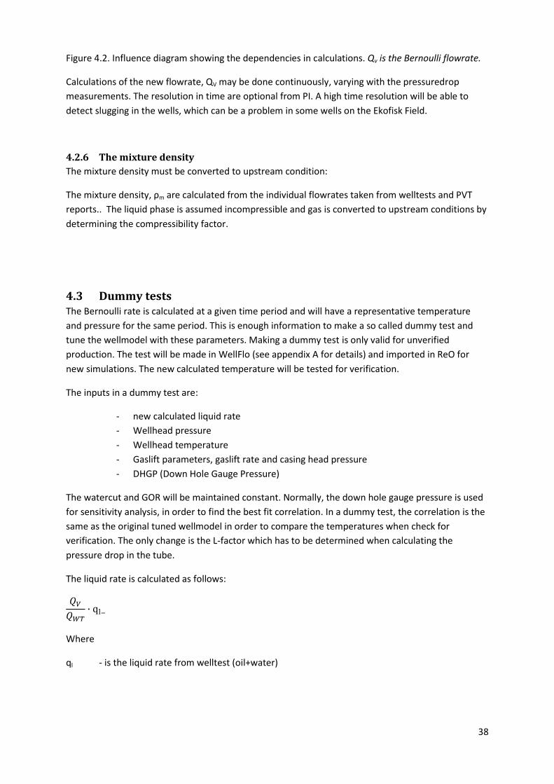
calculation account s for the uncertainties in densities and discharge coefficients. Figure 4.2 is
showing an influence diagram of the dependencies in the process.
Monitoring
CalculateQv
Establish new Kv
38
Figure 4.2. Influence diagram showing the dependencies in calculations. Qv is the Bernoulli flowrate.
Calculations of the new flowrate, QV may be done continuously, varying with the pressuredrop
measurements. The resolution in time are optional from PI. A high time resolution will be able to
detect slugging in the wells, which can be a problem in some wells on the Ekofisk Field.
4.2.6 The mixture density
The mixture density must be converted to upstream condition:
The mixture density, ρm are calculated from the individual flowrates taken from welltests and PVT
reports.. The liquid phase is assumed incompressible and gas is converted to upstream conditions by
determining the compressibility factor.
4.3 Dummy tests The Bernoulli rate is calculated at a given time period and will have a representative temperature
and pressure for the same period. This is enough information to make a so called dummy test and
tune the wellmodel with these parameters. Making a dummy test is only valid for unverified
production. The test will be made in WellFlo (see appendix A for details) and imported in ReO for
new simulations. The new calculated temperature will be tested for verification.
The inputs in a dummy test are:
- new calculated liquid rate
- Wellhead pressure
- Wellhead temperature
- Gaslift parameters, gaslift rate and casing head pressure
- DHGP (Down Hole Gauge Pressure)
The watercut and GOR will be maintained constant. Normally, the down hole gauge pressure is used
for sensitivity analysis, in order to find the best fit correlation. In a dummy test, the correlation is the
same as the original tuned wellmodel in order to compare the temperatures when check for
verification. The only change is the L-factor which has to be determined when calculating the
pressure drop in the tube.
The liquid rate is calculated as follows:
Where
ql - is the liquid rate from welltest (oil+water)

39
Several simulations with both dummy test and the unverified estimates are needed in order to make
a good comparison. The simulations are performed manually, by using historical data representing
the unverified period.
40
5 Results and discussion In the beginning of this examination, a lot of effort was used to find a representative expression of
the mixture density when using the Bernoulli equation at in-situ conditions. Converting flowrates
from standard condition to in-situ, by using PVT data gave a sense of the uncertainties in the
estimation and the risk of not calculate the flowrate by success. Ending up with an expression which
is not involving the densities or the discharge coefficient simplified the procedure and eliminated
some of the uncertainties.
A sensitivity analysis was performed on different densities to see the influence on the calculations.
The purpose was to calculate fluid fractions based on upstream pressure conditions, by estimating a
range of slip and at standard conditions. Using the Bernoulli equation, one has to assume that the
density remains constant. It was of interest to analyze the differences in results. However, this work
was early discharged due another procedure.
The upper and lower temperature limit was at first sat to be 20 degrees Fahrenheit. This seemed to
be to high acceptance for deviation in temperature, resulting in a too large number of verified
normal producing wells. The limits were reduced to only 5 degrees Fahrenheit, which seems to be a
good tolerance in accepted deviation for temperature. For gas lifted, slugging or unstable wells the
tolerance has to be greater due to more various temperatures. For these wells the limit is 10 degrees
Fahrenheit.
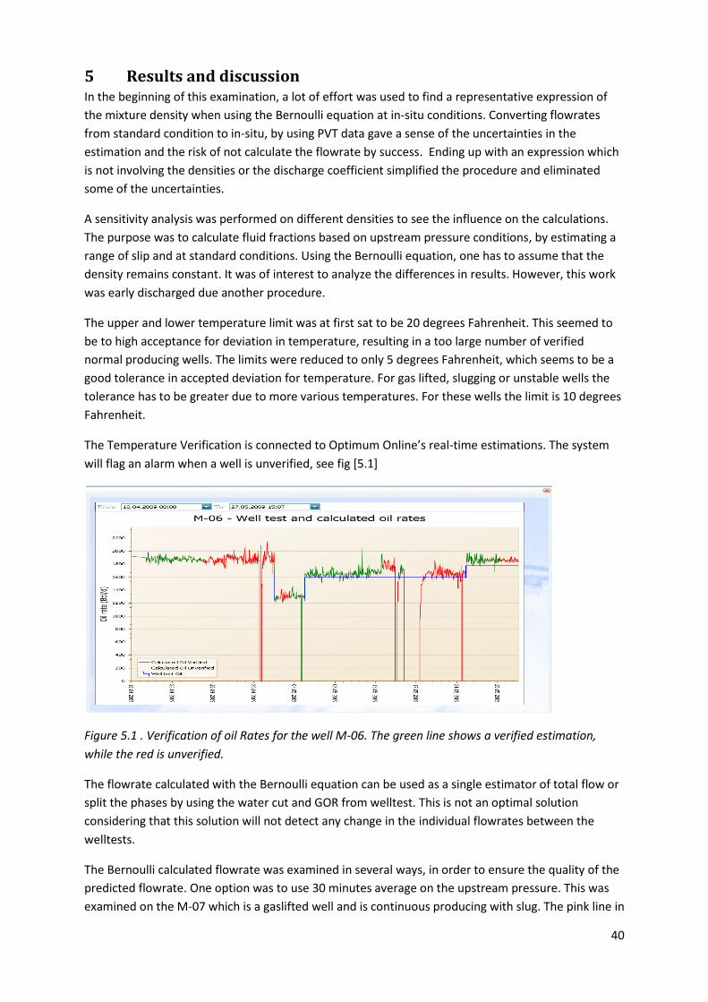
The Temperature Verification is connected to Optimum Online’s real-time estimations. The system
will flag an alarm when a well is unverified, see fig [5.1]
Figure 5.1 . Verification of oil Rates for the well M-06. The green line shows a verified estimation,
while the red is unverified.
The flowrate calculated with the Bernoulli equation can be used as a single estimator of total flow or
split the phases by using the water cut and GOR from welltest. This is not an optimal solution
considering that this solution will not detect any change in the individual flowrates between the
welltests.
The Bernoulli calculated flowrate was examined in several ways, in order to ensure the quality of the
predicted flowrate. One option was to use 30 minutes average on the upstream pressure. This was
examined on the M-07 which is a gaslifted well and is continuous producing with slug. The pink line in
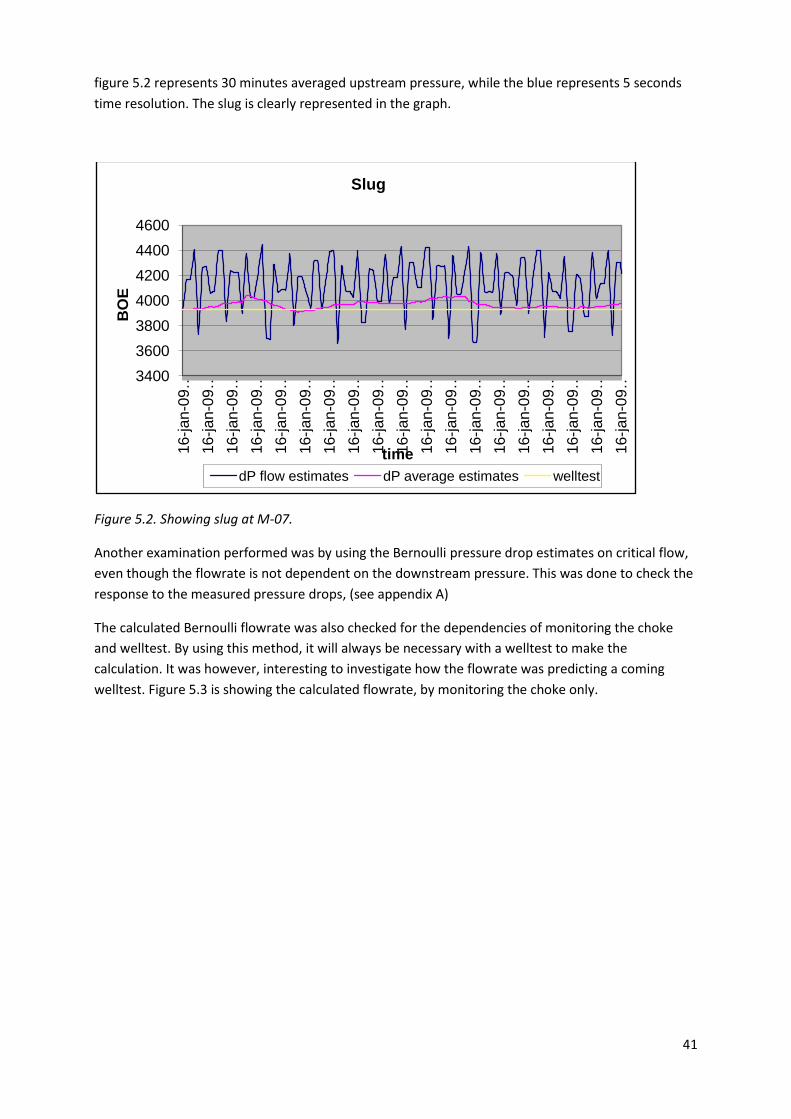
41
figure 5.2 represents 30 minutes averaged upstream pressure, while the blue represents 5 seconds
time resolution. The slug is clearly represented in the graph.
Figure 5.2. Showing slug at M-07.
Another examination performed was by using the Bernoulli pressure drop estimates on critical flow,
even though the flowrate is not dependent on the downstream pressure. This was done to check the
response to the measured pressure drops, (see appendix A)
The calculated Bernoulli flowrate was also checked for the dependencies of monitoring the choke
and welltest. By using this method, it will always be necessary with a welltest to make the
calculation. It was however, interesting to investigate how the flowrate was predicting a coming
welltest. Figure 5.3 is showing the calculated flowrate, by monitoring the choke only.
3400
3600
3800
4000
4200
4400
4600
16-j
an-0
9 …
16-j
an-0
9 …
16-j
an-0
9 …
16-j
an-0
9 …
16-j
an-0
9 …
16-j
an-0
9 …
16-j
an-0
9 …
16-j
an-0
9 …
16-j
an-0
9 …
16-j
an-0
9 …
16-j
an-0
9 …
16-j
an-0
9 …
16-j
an-0
9 …
16-j
an-0
9 …
16-j
an-0
9 …
16-j
an-0
9 …
16-j
an-0
9 …
16-j
an-0
9 …
16-j
an-0
9 …
BO
E
time
Slug
dP flow estimates dP average estimates welltest

42
Figure 5.3. Calculated flowrate by monitoring the choke and not update with the welltests.
The Bernoulli calculated flowrate seems to detect a change in the well performance for sub critical
flow. 14th of May, the well M-06 was about to die. The real-time estimated production was showing
unverified before shut in (see figure 5.5). The predicted Bernoulli flow rate was also showing a
decrease in production, but suddenly a large increase in production (see figure 5.3). Information
from the off shore log was telling that the well was put on gaslift the15th of May, and back as a
normal producer the 18th of May. The reason for a shut in status in Online estimates is the high
wellhead pressure when the well was on gaslift.
At 11th of June, the method of using Bernoulli in predicting flow rate, was programmed in a local
database at Optimum. Results can be seen in appendix A.
M-03 Method Comparision
6000
7000
8000
9000
10000
20090304
20090307
20090310
20090313
20090316
20090318
20090321
20090324
20090327
20090330
20090402
20090404
20090407
20090410
20090413
20090416
20090419
time
BO
E
dP flow estimates Online estimates Welltest

43
Figure 5.4 . The Bernoulli rate at first showing a decrease in flowrate, and then a suddenly increase.
Figure 5.5. The measured temperature (blue line) is falling due to a decrease in production. The red
line is sowing unverified estimates and the well is shut in.
M-06 Bernoulli flow rate
010002000300040005000600070008000
05-m
ai-
06-m
ai-
07-m
ai-
08-m
ai-
09-m
ai-
10-m
ai-
11-m
ai-
12-m
ai-
13-m
ai-
14-m
ai-
15-m
ai-
16-m
ai-
17-m
ai-
18-m
ai-
19-m
ai-
20-m
ai-
21-m
ai-
22-m
ai-
time
BO
E
Bernoulli flow rate Welltest

44
6 Conclusion and Recommendations
1. The use of temperatures to verify real-time estimated production seems to predict a
reasonably change in well performance. Advantage of this method is the ability to improve
the allocation for each single well and detect any deviations in the well behavior. Variations
in temperature may also indicate changes in water cut and GOR. It is important to be aware
of that this method does not capture these changes. However, the deviations in temperature
could be basis for further work in predicting the flux in water cut and GOR.
2. An expression for predicting the flow rate through chokes by using Bernoulli’s equation was
successfully found and seems to have a potential for further development. The flow rate can
be used as a single BOE estimate, or for use in Wellflo as dummy tests. The benefit of only
using the calculated Bernoulli flowrate is the opportunity to use historical data from PI and
analyze special events at any time resolutions. This may be a powerful tool in diagnostics and
planning process. In this analysis, a high time resolution of 5 seconds did detected slug flow. .
A subcritical flow will predict the natural decline in production, slug flow or other unexpected
behavior in the well. It is also possible to split the flow into single phases by assuming
constant GOR and water cut from the well tests.
It is worth mentioning that programming the calculations of the predicted flowrates into a
software and bringing it in real time, could with contribute with the status of the well, when
it is shut in. An interesting survey would then be to compare it to fiscal measurement.
Small variations in flowrates are shown for critical flow. An unverified production could
indicate a change in watercut or GOR. Therefore a pressure drop method is not an alternative
for both calculating the flowrate or in dummy tests. A method that could be worth
investigated, is graphing the wellhead pressure at different choke settings. The flow rate is
found by the intersection of the WPR curve and the choke line.
3. Use of dummy tests in simulations during unverified periods gave a match in temperature.
New dummy tests were imported in the simulation model if the a new unverified
temperature.
4. Monitoring chokes to predict the relationship between the pressure drop and the flow rate
through the choke seems to be a proper application to the temperature verification in
detecting the change in well performance for sub critical flow. Performance of the model was
found to be in good agreement with Optimum Online estimates and in matching new well
tests. Over time, a reduced flow rate was observed as a consequence of decrease in pressure
drop. This was also reflected periodical in the temperature verification, showing real time
estimations starting to deviate from the Bernoulli estimates. Making a dummy test in Wellflo
and import it to the real time model, gave a match within the temperature verification.
Unstable wells, slugging or gaslifted wells needed a better tolerance in temperature
acceptance and may give a reinforced well performance. Especially when putting a normal
well at gas lift, or change the injection rate. By such unforeseen situations, there is need for e
new reference before a new well test and could be worth further investigations.
45
References
1. Michael J. Economides, A. Daniell Hill, Christine Ehling-Economides ” PETROLEUM
PRODUCTION SYSTEMS”. Prentice Hall Petroleum Engineering series. New Jersey 1994. ISBN
0-13-658683-X
2. “A review of Multiphase Flow Through Chokes” S.Rastoin, Z.Schmidt, D.R. Doty. Petroleum
Engineering Department, University of Tulsa. Journal of Energy Resources Technology. 1997
ASME
3. “Predictions of Two-Phase Critical Flow Boundary and Mass Flow Rate Across Chokes”
E.M.Al-safran, SPE, Kuwait University, and M. Kelkar, SPE, University of Tulsa 2007. SPE
109234.
4. PVT analysis. Tor Austad, Universty of Stavanger.
5. Correspondence and conversations with Tore Flåtten, PhD and at the Institute for Energy and
Process, NTNU.
6. Petroleumsproduksjon. Compendium by Erik Skaugen. University of Stavanger.
7. “Well Performance” Golan, M. and Whitson, C. H. 2nd edition 1991.
8. Howard B. Bradley. Petroleum Engineering Handbook. Third printing. Society of Petroleum
Engineers. Richardson, TX, U.S.A. ISBN 1-55563-010-3.
9. User Manual for WellFlo. EPS, Edinburgh Petroleum services.
10. Report ConocoPhillips april 2009.
11. Ahsan, A.R. and Kabir, C.S “Aspects of Wellbore Heat Transfer During Two Phase Flow”. 1994

46
Nomenclature A =cross sectional area [ft2]
Al = cross sectional area occupied with liquid [ft2]
Ar =relaxation distance[ft]
Ag =cross sectional area occupied with gas [ft2]
CHP =casing head pressure [psia]
dP =pressure drop
FD(t) = dimensionless transient heat conduction
g =gravity [ft/s2]
GOR =gas oil ratio [scf/d]
GIR =gas injection rate [scf/d]
ht = forced heat transfer coefficient for the annulus fluid [BTU/hr-ft2°F]
hc = convective heat transfer coefficient for annulus fluid [BTU/hr-ft2-°F]
IPR =inflow performance relation
kcem - is the cement conductivity [BTU/hr-ft2-°F]
Ke =thermal conductivity [BTU/ft D.°F]
kins - is the conductivity of the insulating material [BTU/hr-ft2-°F]
kt = conductivity of the tubing material [BTU/hr-ft2-°F]
PI =productivity index [STB/d-Psia]
Pwf =wellbore flowing pressure [Psia]
Pr =average reservoir pressure [Psia]
Ppr =pseudo reduced pressure[psia]
ppc =pseudo critical pressure [psia]
ql = liquid rate [STB/d]
qo =oil rate [STB/d]
qo max =max oil rate when Pwf=0 [STB/d]
rci = inside radius of the casing [ft]
rco = outside radius of the casing [ft]
Qm =mass flow rate [lb/ft3]
47
QV = Volume flow rate calculated by Bernoulli’s equation *bbl/d+ (v:venturi)
rins = radius outside the insulation material [ft]
rto = outside radius of the tubing [ft]
rti = inside radius of the tubing [ft]
rci =inner pipe diameter [ft]
RT =real-time
S =dimensionless slip ratio
Tpc =pseudo critical temperature [degF]
Tpr =pseudo reduced temperature [degF]
TPR =tubing performance relation
UgS =superficial gas velocity [ft/s]
UlS = superficial liquid velocity [ft/s]
Utf =total heat transfer
Utot =overall heat transfer coefficient [BTU/hr-ft2-°F]
ul =liquid phase velocity [ft/s]
ug =gas phase velocity [ft/s]
WC =water cut, dimensionless
WHP = wellhead pressure [psia]
WHT =wellhead temperature [degF]
ρm = mixture density [lbm/ft3]
αl =dimensionless estimated liquid fraction/no slip fraction
αg =dimensionless estimated gas fraction/no slip fraction
εl =dimensionless true liquid fraction at slip
εg =dimensionless true gas fraction at slip
vc =sonic velocity [ft/s]
vgc =sonic velocity for gas [ft/s]
vlc =sonic velocity for liquid [ft/s]
vm = mixed velocity [ft/s]
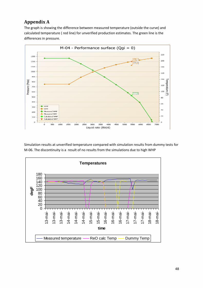
48
Appendix A The graph is showing the difference between measured temperature (outside the curve) and
calculated temperature ( red line) for unverified production estimates. The green line is the
differences in pressure.
Simulation results at unverified temperature compared with simulation results from dummy tests for
M-06. The discontinuity is a result of no results from the simulations due to high WHP
Temperatures
020406080
100120140160180
13-m
ai-
13-m
ai-
13-m
ai-
14-m
ai-
14-m
ai-
14-m
ai-
15-m
ai-
15-m
ai-
16-m
ai-
16-m
ai-
16-m
ai-
17-m
ai-
17-m
ai-
17-m
ai-
18-m
ai-
18-m
ai-
time
deg
F
Measured temperature ReO calc Temp Dummy Temp

49
Some information about the wells:
Well Flow Average* GOR
Average* WC accep. dev. ∆T
[scf/d] % upper&lower lim [degF] Comment
M-01 sub-critical 3208 9.94 10
M-02 sub-critical 1988.4 74.96 5
M-03 critical 1117.6 37.92 5
M-04 sub-critical 1083.3 21.34 10
M-05 critical 792 24.17 5
M-06 sub-critical 1227.8 3.9 10
M-07 critical 517.4 33.9 10 slug
M-08 sidetracked
M-09 critical 5181.2 4.98 5
M-10 sub-critical 2601 42.6 5 variations in WT
M-11 critical 1144.7 70.1 5
M-12 critical 1212.6 11.4 5
M-13 sidetracked
M-14 critical 1143.9 29.2 5
M-15 critical 1611.2 34.08 5
*Average from several welltests
Method Comparision 1. The graph is showing Bernoulli flow rate, without monitoring the choke size and not included with
coming welltest:
M-09 Method comparision
1500
2000
2500
3000
3500
4000
20
09
05
07
20
09
05
08
20
09
05
09
20
09
05
10
20
09
05
11
20
09
05
12
20
09
05
13
20
09
05
14
20
09
05
15
20
09
05
16
20
09
05
17
20
09
05
18
20
09
05
20
20
09
05
21
20
09
05
22
20
09
05
23
20
09
05
24
time
BO
E
dP flow Online Estimates Welltest

50
2. The next graph is showing the same well in the same time period, but is monitoring the choke:
3. This graph includes both monitoring the choke and is updated with coming welltests:
1. Calculated Bernoulli flowrate, without monitoring the choke or new welltests:
M-09 Method Comparision
1500
2000
2500
3000
3500
4000
20
09
05
07
20
09
05
08
20
09
05
09
20
09
05
10
20
09
05
11
20
09
05
12
20
09
05
13
20
09
05
14
20
09
05
15
20
09
05
16
20
09
05
17
20
09
05
18
20
09
05
19
20
09
05
20
20
09
05
21
20
09
05
22
20
09
05
23
20
09
05
24
20
09
05
25
time
BO
E
dP flow estimates Online Estimates Welltest
M-09 Method Comparision
1500
2000
2500
3000
3500
4000
20
09
05
07
20
09
05
08
20
09
05
09
20
09
05
10
20
09
05
11
20
09
05
12
20
09
05
13
20
09
05
14
20
09
05
15
20
09
05
16
20
09
05
17
20
09
05
18
20
09
05
19
20
09
05
20
20
09
05
21
20
09
05
22
20
09
05
23
20
09
05
24
20
09
05
25
dP flow estimates Online estimates Welltest
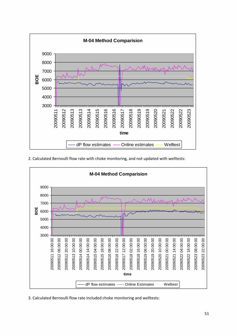
51
2. Calculated Bernoulli flow rate with choke monitoring, and not updated with welltests:
3. Calculated Bernoulli flow rate included choke monitoring and welltests:
M-04 Method Comparision
3000
4000
5000
6000
7000
8000
900020090511
20090512
20090513
20090513
20090514
20090515
20090516
20090516
20090517
20090518
20090519
20090519
20090520
20090521
20090522
20090522
20090523
time
BO
E
dP flow estimates Online estimates Welltest
M-04 Method Comparision
3000
4000
5000
6000
7000
8000
9000
20090511 1
6:0
0:0
0
20090512 0
6:0
0:0
0
20090512 2
0:0
0:0
0
20090513 1
0:0
0:0
0
20090514 0
0:0
0:0
0
20090514 1
4:0
0:0
0
20090515 0
4:0
0:0
0
20090515 1
8:0
0:0
0
20090516 0
8:0
0:0
0
20090516 2
2:0
0:0
0
20090517 1
2:0
0:0
0
20090518 0
2:0
0:0
0
20090518 1
6:0
0:0
0
20090519 0
6:0
0:0
0
20090519 2
0:0
0:0
0
20090520 1
0:0
0:0
0
20090521 0
0:0
0:0
0
20090521 1
4:0
0:0
0
20090522 0
4:0
0:0
0
20090522 1
8:0
0:0
0
20090523 0
8:0
0:0
0
20090523 2
2:0
0:0
0
time
BO
E
dP flow estimates Online Estimates Welltest
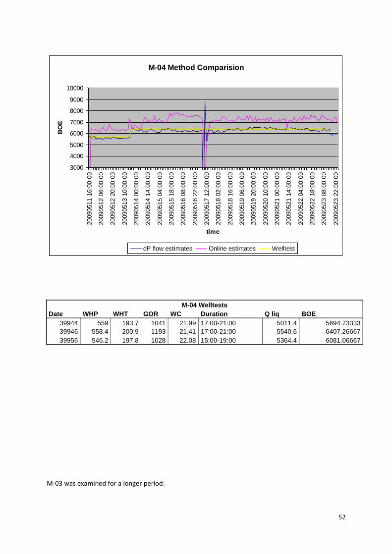
52
M-04 Welltests
Date WHP WHT GOR WC Duration Q liq BOE
39944 559 193.7 1041 21.99 17:00-21:00 5011.4 5694.73333
39946 558.4 200.9 1193 21.41 17:00-21:00 5540.6 6407.26667
39956 546.2 197.8 1028 22.08 15:00-19:00 5364.4 6081.06667
M-03 was examined for a longer period:
M-04 Method Comparision
3000
4000
5000
6000
7000
8000
9000
1000020090511 1
6:0
0:0
0
20090512 0
6:0
0:0
0
20090512 2
0:0
0:0
0
20090513 1
0:0
0:0
0
20090514 0
0:0
0:0
0
20090514 1
4:0
0:0
0
20090515 0
4:0
0:0
0
20090515 1
8:0
0:0
0
20090516 0
8:0
0:0
0
20090516 2
2:0
0:0
0
20090517 1
2:0
0:0
0
20090518 0
2:0
0:0
0
20090518 1
6:0
0:0
0
20090519 0
6:0
0:0
0
20090519 2
0:0
0:0
0
20090520 1
0:0
0:0
0
20090521 0
0:0
0:0
0
20090521 1
4:0
0:0
0
20090522 0
4:0
0:0
0
20090522 1
8:0
0:0
0
20090523 0
8:0
0:0
0
20090523 2
2:0
0:0
0
time
BO
E
dP flow estimates Online estimates Welltest
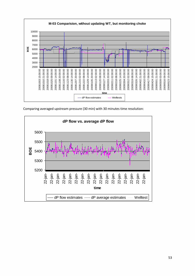
53
Comparing averaged upstream pressure (30 min) with 30 minutes time resolution:
M-03 Comparision, without updating WT, but monitoring choke
2000
3000
4000
5000
6000
7000
8000
9000
10000
20
08
10
03
15
:00
:00
20
08
10
10
21
:00
:00
20
08
10
18
03
:00
:00
20
08
10
25
09
:00
:00
20
08
11
01
14
:00
:00
20
08
11
08
20
:00
:00
20
08
11
16
02
:00
:00
20
08
11
23
08
:00
:00
20
08
11
30
14
:00
:00
20
08
12
07
20
:00
:00
20
08
12
15
02
:00
:00
20
08
12
22
08
:00
:00
20
08
12
29
14
:00
:00
20
09
01
05
20
:00
:00
20
09
01
13
02
:00
:00
20
09
01
20
08
:00
:00
20
09
01
27
14
:00
:00
20
09
02
03
20
:00
:00
20
09
02
11
02
:00
:00
20
09
02
18
08
:00
:00
20
09
02
25
14
:00
:00
20
09
03
04
20
:00
:00
20
09
03
12
02
:00
:00
20
09
03
19
08
:00
:00
20
09
03
26
14
:00
:00
20
09
04
02
21
:00
:00
20
09
04
10
03
:00
:00
20
09
04
17
09
:00
:00
20
09
04
24
15
:00
:00
20
09
05
01
21
:00
:00
20
09
05
09
03
:00
:00
20
09
05
16
09
:00
:00
20
09
05
23
15
:00
:00
time
BO
E
dP flow estimates Welltests
dP flow vs. average dP flow
5200
5300
5400
5500
5600
22-jan-
22-jan-
22-jan-
22-jan-
22-jan-
22-jan-
22-jan-
22-jan-
22-jan-
22-jan-
22-jan-
22-jan-
22-jan-
22-jan-
22-jan-
22-jan-
22-jan-
time
BO
E
dP flow estimates dP average estimates Welltest

54
M-05 dP vs. dP average
4000
5000
6000
7000
19
-ja
n-0
9
19
-ja
n-0
9
19
-ja
n-0
9
19
-ja
n-0
9
20
-ja
n-0
9
20
-ja
n-0
9
20
-ja
n-0
9
21
-ja
n-0
9
21
-ja
n-0
9
21
-ja
n-0
9
21
-ja
n-0
9
22
-ja
n-0
9
22
-ja
n-0
9
22
-ja
n-0
9
23
-ja
n-0
9
23
-ja
n-0
9
23
-ja
n-0
9
23
-ja
n-0
9
24
-ja
n-0
9
24
-ja
n-0
9
24
-ja
n-0
9
time
BO
E
dP flow estimates dP avg. Flow estimates Welltest
55
Predicted flowrates from Bernoulli equation.

56

57
M-06
58
59

60
Dummy Tests Dates of performing simulations with on-line values and dummy tests implemented in the network
model.
Simulations performed with dummy tests for unverified periods
Well Date
M-01 06.feb 10.mar 01.apr
M-02 21.mar
M-03 03.jun
M-04 05.mar 10.mar 20.mar 21.mai
M-05 29.mar
M-06 29.mai 01.jun 14.jun
M-07 24.mar 27.apr
M-09 01.jan 05.mar 28.mai
M-10 01.mar 03.apr 05.mai
M-11 28.12.2008
M-12 29.12.2008
M-14 30.12.2008
M-15 31.12.2008 12.jan 10.apr
Example of results from simulations:
Accepted deviation:10 degF Measured T RT calc T* Dummy T
M-07 Date Time [degF] [degF] [degF]
30.04.2009 06:00 186.67 171.5288 186.67
30.04.2009 08:00 185.97 172.1696 185.97
30.04.2009 10:00 186.15 172.4612 186.15
30.04.2009 12:00 186.33 171.0698 186.33
30.04.2009 14:00 186.03 172.1246 186.03
30.04.2009 16:00 187.12 170.9762 187.12
30.04.2009 18:00 186.59 172.436 186.59
30.04.2009 20:00 186.32 172.1732 186.32
30.04.2009 22:00 186.29 172.166 186.22
01.05.2009 00:00 186.25 172.1498 186.14
01.05.2009 02:00 186.28 172.175 186.17
01.05.2009 04:00 186.49 171.6026 186.17
01.05.2009 06:00 186.26 171.986 186.01
01.05.2009 08:00 186.42 172.256 186.3
01.05.2009 10:00 186.45 171.5612 186.33
01.05.2009 12:00 186.59 172.571 186.52
T*= unverified temperature.
In addition, it will be given results of oil rate, water rate and gas rate for each well.

61
Tuning Procedure The diagram shows the tuning procedure in WellFlo. The procedure does not include building the
well with equipments, well inclination and PVT data (gravity, API etc.).
Step 1: Input parameters
The first input in the tuning procedure is the fluid parameters from well test results;
GOR, Water Cut and Liquid Rate. This is done in three different windows:

62
Gas Lift Data: If the well is on gas lift, the gas injection rate and the CHP has to be updated.
If not the gas lift valve is set to be not active.

63
Nodal Analysis Control- Pressure Drop Mode: Update WHP, WHT and QL.

64
Step 2: CALCULATION AND TUNING
The tuning procedure depends on if down hole gauge pressure is available.
If not: The pressure is calculated at the Mid. Perforation node and then inserted to the
Reservoir control under Test Pressure 1 in order to find the operating point.
If the data is to be tuned against measured gauge pressure, the pressure is tuned with L-factor
until it matches using the Gauge Carrier as the Solution node. This is done by loading a dvp-file
(depth versus pressure) to run sensitivities and find the best fit L-factor in the correlations.
New pressure is calculated at the mid perforation, with the additional L-factor before added
into Reservoir Control. Finely the Operating point, giving the deliverability, is calculated.

65

66
Optimizing procedure in ReO
1. Chooce platform. Here, MMan represents the Mike platform.

67
2. Select the well and chose import WellFlo file.
3.
Click on the optimization tab, and select optimize
68
4. When simulation is successes, there is an option to click on the well and read results:

69
Simulation results and Temperature Verification

70
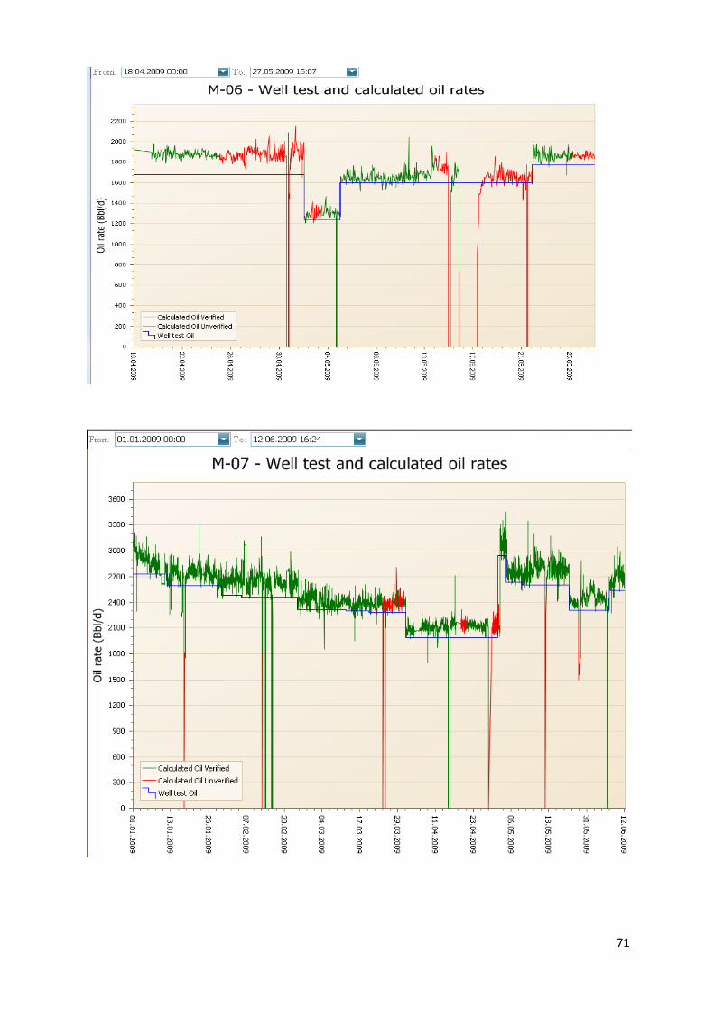
71

72

73

74
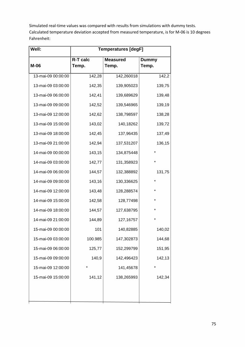
75
Simulated real-time values was compared with results from simulations with dummy tests.
Calculated temperature deviation accepted from measured temperature, is for M-06 is 10 degrees
Fahrenheit:
Well: Temperatures [degF]
M-06
R-T calc
Temp.
Measured
Temp.
Dummy
Temp.
13-mai-09 00:00:00 142,28 142,260018 142,2
13-mai-09 03:00:00 142,35 139,905023 139,75
13-mai-09 06:00:00 142,41 139,689629 139,48
13-mai-09 09:00:00 142,52 139,546965 139,19
13-mai-09 12:00:00 142,62 138,798597 138,28
13-mai-09 15:00:00 143,02 140,18262 139,72
13-mai-09 18:00:00 142,45 137,96435 137,49
13-mai-09 21:00:00 142,94 137,531207 136,15
14-mai-09 00:00:00 143,15 134,875448 *
14-mai-09 03:00:00 142,77 131,358923 *
14-mai-09 06:00:00 144,57 132,388892 131,75
14-mai-09 09:00:00 143,16 130,336625 *
14-mai-09 12:00:00 143,48 128,288574 *
14-mai-09 15:00:00 142,58 128,77498 *
14-mai-09 18:00:00 144,57 127,638795 *
14-mai-09 21:00:00 144,89 127,16757 *
15-mai-09 00:00:00 101 140,82885 140,02
15-mai-09 03:00:00 100.985 147,302873 144,68
15-mai-09 06:00:00 125,77 152,299799 151,95
15-mai-09 09:00:00 140,9 142,496423 142,13
15-mai-09 12:00:00 * 141,45678 *
15-mai-09 15:00:00 141,12 138,265993 142,34

76
Appendix B Data sources from PI:
Upstr P Downstr. P Choke size Temp
[barg] [barg] [%] [degC]
_M-43-PT-10511 _M-43-PT-10514
_M-43-ZT-10512
_M-43-TT-10513
80.50926971 22.2599678 11.60000038 87.84079742
80.45629883 22.47626305 11.60000038 87.72499847
80.32499695 22.30355453 11.60000038 87.61294556
80.27204895 22.18118858 11.60000038 87.5687027
80.22485352 22.76850319 11.60000038 87.50791168
80.16261292 22.56083488 11.60000038 87.43520355
80.04060364 22.22386169 11.60000038 87.39897156
80.12809753 22.32917595 11.60000038 87.57767487
80.09363556 22.82262802 11.60000038 87.6475296
80.0591507 22.54389954 11.60000038 87.69826508
80.04060364 22.58600044 11.60000038 87.71418762
79.97499847 22.22868538 11.60000038 87.7908783
79.89678192 22.53261566 11.60000038 87.76143646
79.87823486 22.14545059 11.60000038 87.79772186
79.82189941 22.21612549 11.60000038 87.80644989
79.7687912 22.76906013 11.60000038 87.80750275
79.71250153 22.57664299 11.60000038 87.85559845
79.73439789 22.9138813 11.60000038 87.80278778
79.69059753 22.92790604 11.60000038 87.79667664
79.63762665 22.50828934 11.60000038 87.79772186
79.55010223 22.80681038 11.60000038 87.73587036
79.48455048 22.00694466 11.60000038 87.70547485
79.46261597 23.04554176 11.60000038 87.7329483
79.36250305 22.65449333 11.60000038 87.68953705
79.36250305 22.60722923 11.60000038 87.69726563
79.2842865 22.68940926 11.60000038 87.68662262
79.26571655 22.65851021 11.60000038 87.69059753
79.07810211 22.38804245 11.60000038 87.74958038
79.09075165 22.62930679 11.60000038 87.79088593
79.00279236 22.79326057 11.60000038 87.78462982
Arrangement of data sources:
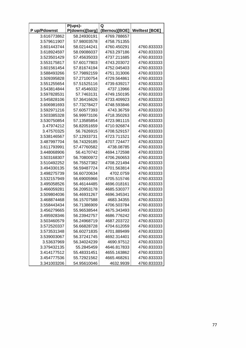
77
P up/Pdownst P(ups)-P(downs)[barg]
Q (Bernou)[BOE] Welltest [BOE]
3.616773862 58.24930191 4769.788657
3.579611907 57.98003578 4758.751355
3.601443744 58.02144241 4760.450291 4760.833333
3.618924597 58.09086037 4763.297186 4760.833333
3.523501429 57.45635033 4737.211685 4760.833333
3.553175817 57.60177803 4743.203072 4760.833333
3.601561454 57.81674194 4752.045403 4760.833333
3.588493266 57.79892159 4751.313006 4760.833333
3.509395828 57.27100754 4729.564861 4760.833333
3.551255654 57.51525116 4739.639217 4760.833333
3.543814844 57.4546032 4737.13966 4760.833333
3.597828531 57.7463131 4749.150195 4760.833333
3.545828106 57.36416626 4733.409923 4760.833333
3.606981693 57.73278427 4748.593846 4760.833333
3.592971216 57.60577393 4743.36759 4760.833333
3.503385328 56.99973106 4718.350263 4760.833333
3.530750854 57.13585854 4723.981115 4760.833333
3.47974212 56.82051659 4710.926874 4760.833333
3.47570325 56.7626915 4708.529157 4760.833333
3.538146567 57.12933731 4723.711521 4760.833333
3.487997704 56.74329185 4707.724477 4760.833333
3.611793991 57.47760582 4738.08785 4760.833333
3.448068906 56.4170742 4694.172598 4760.833333
3.503168307 56.70800972 4706.260653 4760.833333
3.510492252 56.75527382 4708.221494 4760.833333
3.494330135 56.59487724 4701.563814 4760.833333
3.498275739 56.60720634 4702.0759 4760.833333
3.532157949 56.69005966 4705.515746 4760.833333
3.495058526 56.46144485 4696.018161 4760.833333
3.466059281 56.20953178 4685.530377 4760.833333
3.509804036 56.46931267 4696.345341 4760.833333
3.468874468 56.15707588 4683.34355 4760.833333
3.558443434 56.71386909 4706.503784 4760.833333
3.456279665 55.96538544 4675.343493 4760.833333
3.495928346 56.23942757 4686.776242 4760.833333
3.503460579 56.24968719 4687.203722 4760.833333
3.572520337 56.66828728 4704.612059 4760.833333
3.573531348 56.60271835 4701.889499 4760.833333
3.539003067 56.37241745 4692.314401 4760.833333
3.53637969 56.34024239 4690.97512 4760.833333
3.379432135 55.2845459 4646.817833 4760.833333
3.414177512 55.48331451 4655.163862 4760.833333
3.454777536 55.72921562 4665.468261 4760.833333
3.341003206 54.95610046 4632.9939 4760.833333