Embed Size (px)
Citation preview
IFC workshop on “Combining micro and macro statistical data for financial stability analysis. Experiences, opportunities and challenges”
Warsaw, Poland, 14-15 December 2015
Determinants of credit in the Polish banking sector before and after the GFC according to information
from the NBP Senior Loan Officer Survey. Does supply or demand matter?1
Zuzanna Wośko, Narodowy Bank Polski (Poland)
1 This paper was prepared for the meeting. The views expressed are those of the author and do not necessarily reflect the views of the BIS or the central banks and other institutions represented at the meeting.
1
Irving Fisher Committee Workshop: Combining micro and macro statistical data for
financial stability analysis. Experiences, opportunities and challenges.
Title:
Determinants of credit in Polish banking sector before and after the Great Financial
Crisis according to information from Senior Loan Officer Opinion Survey data. Does
supply or demand matter?
Zuzanna Wośko1
Abstract
The paper investigates the problem of most important determinants of bank lending in Poland
according to qualitative information of banks from the Senior Loan Officer Opinion Survey.
The analysis takes into consideration banks’ answers on the purpose of the change of their
lending before and after the crisis. The research which bases on the panel regressions as well
as disequilibrium econometrics models allows to decide, which factors – supply or demand
had more important influence on lending growth in particular periods of time. Estimated
models use bank-level and aggregated quarterly data concerning three loan segments –
corporate, housing and consumer from the half of 2005 to the end of 2014.
Key words: credit growth, senior loan officers opinion survey, demand for loans, supply of
loans, credit growth modelling
JEL: E51, G21, G01
1 Narodowy Bank Polski, Financial Stability Department / Warsaw School of Economics, Institute of
Econometrics
2
1. Introduction
The sharp decline in world economic activity during the late of the last decade, which is
generally considered the largest downturn since the Great Depression also influenced the
Polish banking system and its credit dynamics. Following the world financial crisis, banks
curbed supply of loans by considerably tightening the standards and terms of granting them.
Before the crisis, the lending growth in Poland was strong, most notably due to housing loans,
which was the consequence of both households’ rising demand for dwellings, supported by
the increasing availability of credit and its relatively low cost, and limited supply on the
residential property market which elevated prices. The price rise caused a feedback in the
form of growing demand, triggered by, among others, an expected further price rise, which in
turn stimulated higher demand for loans.
A significant role in this process was played by strong easing of standards and terms of
granting loans by banks and the related low loan spreads observed in the pre-crisis period.
This development stemmed from strong competition among banks, leading some institutions
to focus on raising a market share at the expense of diligent credit risk assessment (Financial
Stability Report. July 2010., p. 35).
The accumulation of imbalances has been disrupted by the last financial crisis. Due to
tightening the standards and terms of granting loans. Demand, particularly from enterprises,
also fell.
After a period of tightened policy, from 2011 one could observe the start of a gradual process
of easing the standards and terms of granting loans by banks.
This paper investigates the problem of most important determinants of bank lending in Poland
before and after the crisis. The key issue is the role of demand and supply factors in this
process – if the demand or the supply was the main driver of lending growth? Or, maybe, both
factors influenced the credit in the same way?
To achieve this research goal two kinds of approach were applied. Both were using the
qualitative information of banks from the Senior Loan Officer Opinion Survey. However the
first one, on aggregated data, supported with other banking and macro data leads to the
conclusions about dominations of regimes in particular periods of time – demand or supply.
Here, disequilibrium econometrics methodology was used. The second one bases on the panel
regressions. Panel models are estimated on bank-level quarterly data. The conclusions on the

3
possible impact of different factors are made using significance test of regressors in two
subsamples.
Both approaches consider three loan segments – consumer, housing and corporate from the
half of 2005 to the end of 2014.
The structure of the paper is as follows: chapter 2 summarizes literature on assessing the
impact of demand and supply factors on credit growth, chapter 3 describes econometric
methodology applied to the research. Detailed information on empirical part of the paper are
included into chapter 4 and 5, where the data and results of the analysis are included. The
most important findings are collected in Conclusions.
2. Literature
Estimation of credit demand and supply has become a key issue of many economic
publications. They present not only very wide range of methodologies but also applications to
many countries. But the operational goals of researchers can vary.
Some authors aim at receiving very general information about influence of demand-side and
supply-side variables on credit growth. Others want to find exact trajectories of non-
observable demand and supply, and finally, there are some trying to receive a zero-one
answer about dominating regime for particular time unit.
Vast literature on loan demand-supply decomposition can be classified according to
granularity of data and quantitative methodologies which have been applied.
Aggregated data are usually used in disequilibrium econometrics models, which consist of
demand and supply linear equations together with optimization function which defines
observable volume of credit as minimum of demand and supply. Such approach can be found
in Laffont & Garcia (1977), Sealey (1979), Ito & Ueda (1981), Stenius (1983), Artus (1984),
Martin (1990), Pazarbasioglu (1997), Ghosh and Ghosh (1999), Hurlin & Kierzenkowski
(2002), Burdeau (2014). The aim of mentioned papers were, amongst others, the analysis of
credit crunch in particular country (Canada, USA, Japan, Finland, Korea, Indonesia,
Thailand) or the investigation of monetary transmission channel (for example, Poland in
Hurlin & Kierzenkowski 2002).
Another tool of decomposing the supply and demand for loans in order to investigate
monetary channels was also done in the literature by using VECM (Vector of Error

4
Correction Models) methodology. Imposing appropriate economic restrictions on variables
and then finding cointegrating vectors can reveal quantitatively unobservable demand and
supply side. Such research were presented by, for example, Kakes (2000), Calza (2006),
Mello & Pisu (2009), Łyziak et al. (2014).
There are also relatively new approaches to disentangling supply and demand of loans such as
Dynamic Factor Models (DFM). Balke, Zeng (2013) applied such methodology, in which the
demand and supply of credit are one of the unobservable common factors in the model using
65 macro and financial variables of quarterly and monthly frequency.
However there is much less research on demand and supply of loans based on panel data. One
of most known research is Del Giovane, Eramo, Nobili (2010) who used bank-level data from
Eurosystem Bank Lending Survey – the answers of banks on the demand and supply of
loans. Asea, Blomberg (1997) estimated two regimes of lending growth - high and low risk in
the model, where the margin on loans in a particular bank depends on the real cost of
financing of the bank, the share of risky loans in the bank and the set of macroeconomic
variables. Brown, Kirschenmann, Ongena (2010) used two logit panel models - firms’
decisions to request FX loans and banks’ decision to grant FX loans. The first equation can be
regarded as the approximation of loan demand and the second as realized demand.
This paper uses two different approaches from the literature to Polish data. On aggregate data
the disequilibrium econometrics approach has been used and on disaggregated, bank-level
data somewhat similar analysis to Del Giovane, Eramo, Nobili (2010) has been applied.
3. Methodology
As mentioned above, in this paper the econometric framework of modelling credit dynamics
includes two approaches. The first one is time series regression on aggregated data with the
use of disequilibrium econometric approach (regime-switching model) and the second one is
panel regression on disaggregated (bank level) data.
Disequilibrium approach mentioned in previous chapter is usually applied to aggregated data.
It bases on the system of separate demand and supply equations together with optimization
function which defines observable volume of credit as minimum of demand and supply:
5
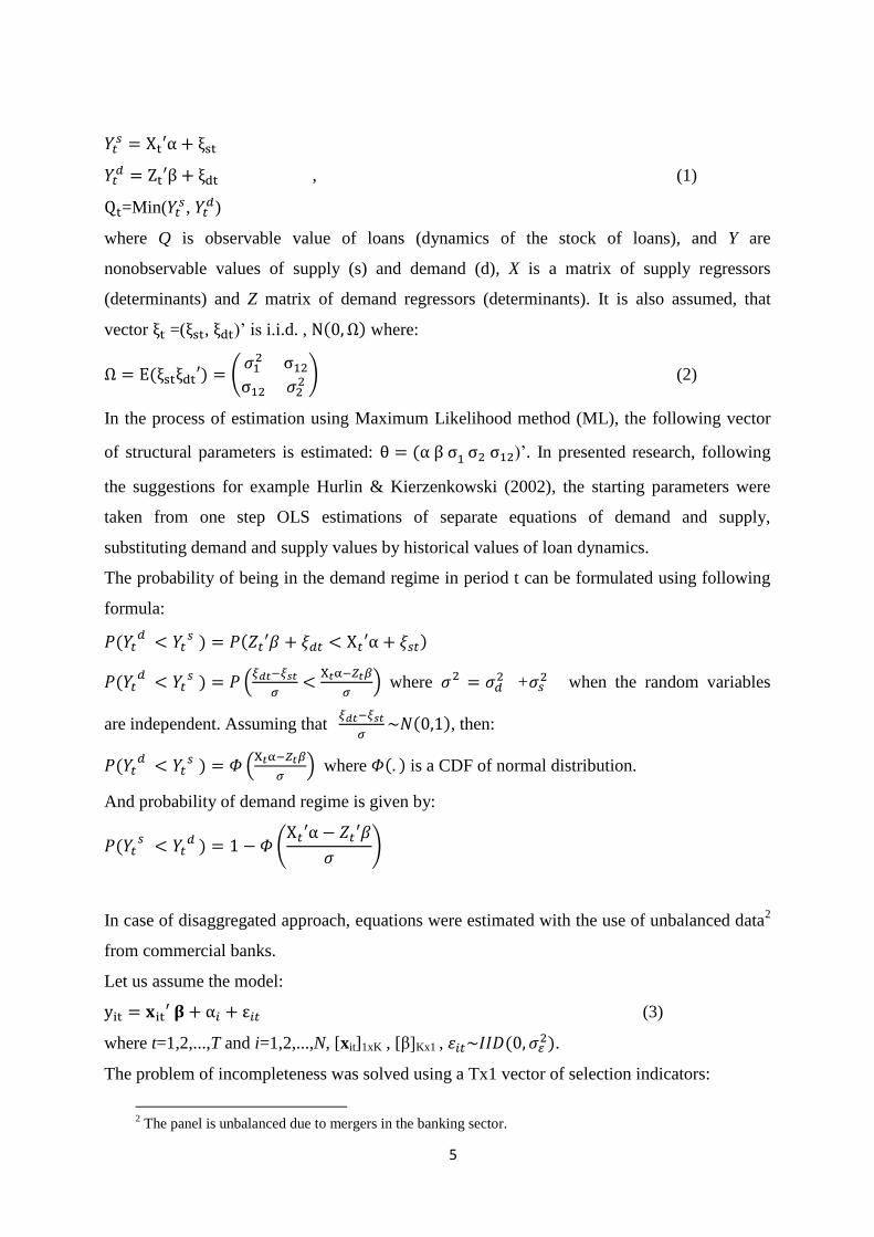
𝑌𝑡𝑠 = Xt′α + ξst
𝑌𝑡𝑑 = Zt′β + ξdt , (1)
Qt=Min(𝑌𝑡𝑠, 𝑌𝑡
𝑑)
where Q is observable value of loans (dynamics of the stock of loans), and Y are
nonobservable values of supply (s) and demand (d), X is a matrix of supply regressors
(determinants) and Z matrix of demand regressors (determinants). It is also assumed, that
vector ξt =(ξst, ξdt)’ is i.i.d. , N(0, Ω) where:
Ω = E(ξstξdt′) = (𝜎1
2 σ12
σ12 𝜎22 ) (2)
In the process of estimation using Maximum Likelihood method (ML), the following vector
of structural parameters is estimated: θ = (α β σ1 σ2 σ12)’. In presented research, following
the suggestions for example Hurlin & Kierzenkowski (2002), the starting parameters were
taken from one step OLS estimations of separate equations of demand and supply,
substituting demand and supply values by historical values of loan dynamics.
The probability of being in the demand regime in period t can be formulated using following
formula:
𝑃(𝑌𝑡𝑑 < 𝑌𝑡
𝑠 ) = 𝑃(𝑍𝑡′𝛽 + 𝜉𝑑𝑡 < X𝑡′α + 𝜉𝑠𝑡)
𝑃(𝑌𝑡𝑑 < 𝑌𝑡
𝑠 ) = 𝑃 (𝜉𝑑𝑡−𝜉𝑠𝑡
𝜎<
X𝑡α−𝑍𝑡𝛽
𝜎) where 𝜎2 = 𝜎𝑑
2 +𝜎𝑠2 when the random variables
are independent. Assuming that 𝜉𝑑𝑡−𝜉𝑠𝑡
𝜎~𝑁(0,1), then:
𝑃(𝑌𝑡𝑑 < 𝑌𝑡
𝑠 ) = 𝛷 (X𝑡α−𝑍𝑡𝛽
𝜎) where 𝛷(. ) is a CDF of normal distribution.
And probability of demand regime is given by:
𝑃(𝑌𝑡𝑠 < 𝑌𝑡
𝑑 ) = 1 − 𝛷 (X𝑡′α − 𝑍𝑡′𝛽
𝜎)
In case of disaggregated approach, equations were estimated with the use of unbalanced data2
from commercial banks.
Let us assume the model:
yit = 𝐱it′ 𝛃 + α𝑖 + ε𝑖𝑡 (3)
where t=1,2,...,T and i=1,2,...,N, [xit]1xK , [β]Kx1 , 𝜀𝑖𝑡~𝐼𝐼𝐷(0, 𝜎𝜀2).
The problem of incompleteness was solved using a Tx1 vector of selection indicators:
2 The panel is unbalanced due to mergers in the banking sector.

6
si = (si1, … , siT)′, where sit = 1 if (xit, yit) is observed and zero otherwise. Such indicators
are included into the parameters’ estimator.
Equations of lending growth were estimated with the use of the OLS while allowing the
standard errors (and variance–covariance matrix of the estimates) to be consistent when the
disturbances from each observation are not independent, and specifically, allowing the
standard errors to be robust to each bank having a different variance of the disturbances and to
each bank’s observations being correlated with those of the other banks through time.
Nevertheless, some of the equations are dynamic. Dynamic panel regression with AR(m) can
be presented as:
yit = δyi,t−m + xit′ β + αi + εit (4)
where δ is a scalar. The issue of estimator’s properties in dynamic unbalanced panel
regressions was more developed in Wośko (2015).
4. Data
Almost all the research cited in chapter 2 on demand and supply of loans use change of the
stock of loans to approximate flow of new credit. However it should be considered that such
measurement is biased, amongst others, by repayments, loan sale transactions and
securitization. For example, Giovane et al. (2010) excluded securitization from the dynamics
of credit and it improved the significance of the statistical influence of variables from the
SLOS.
In order to identify regimes correctly, first of all, one need to exclude the rate of depreciation
of loans (amortization). But reporting bank standards in Poland does not allow for accurate
separation of repayment of loans. The same problem occurs in case of loan sale transactions.
Lending growth can be distorted especially in case of consumer loans. In this segment of
loans sale transactions are common in Poland, contrary to corporate loans. Information about
loan sale transactions is rather poor.
Therefore we have to use simple measure of new loans using quarterly difference of stock of
loans in case of aggregated data and quarterly rate of growth in case of disaggregated data
ignoring above mentioned problem. But we are aware of consequences of such simplification.
Main source of data to the research is Senior Loan Officers Opinion Survey (SLOS). SLOS is
regularly carried out by Narodowy Bank Polski since 2003 Q4. It is directed at
CEOs/executives chairing credit committees at commercial banks and the content is similar to
analogous ECB and Fed surveys. Aggregate results are presented in the form of diffusion
7
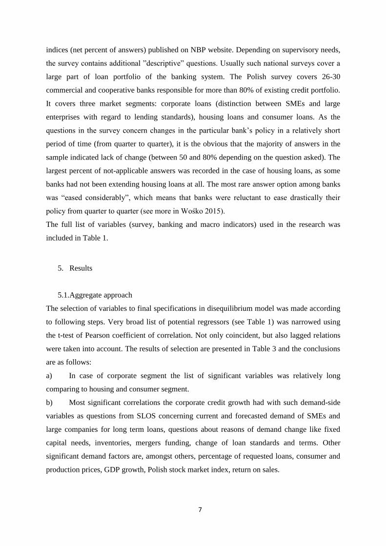
indices (net percent of answers) published on NBP website. Depending on supervisory needs,
the survey contains additional ”descriptive” questions. Usually such national surveys cover a
large part of loan portfolio of the banking system. The Polish survey covers 26-30
commercial and cooperative banks responsible for more than 80% of existing credit portfolio.
It covers three market segments: corporate loans (distinction between SMEs and large
enterprises with regard to lending standards), housing loans and consumer loans. As the
questions in the survey concern changes in the particular bank’s policy in a relatively short
period of time (from quarter to quarter), it is the obvious that the majority of answers in the
sample indicated lack of change (between 50 and 80% depending on the question asked). The
largest percent of not-applicable answers was recorded in the case of housing loans, as some
banks had not been extending housing loans at all. The most rare answer option among banks
was “eased considerably”, which means that banks were reluctant to ease drastically their
policy from quarter to quarter (see more in Wośko 2015).
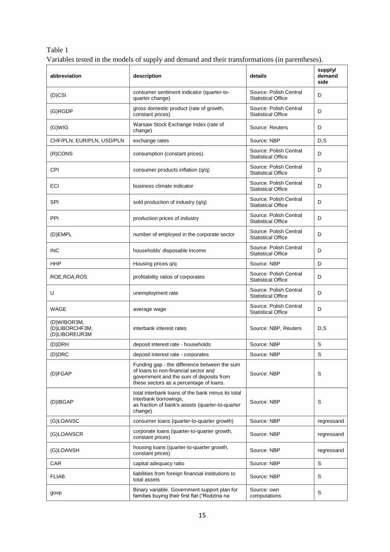
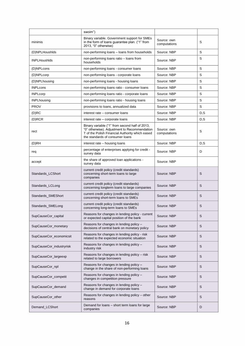
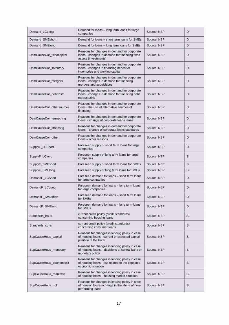
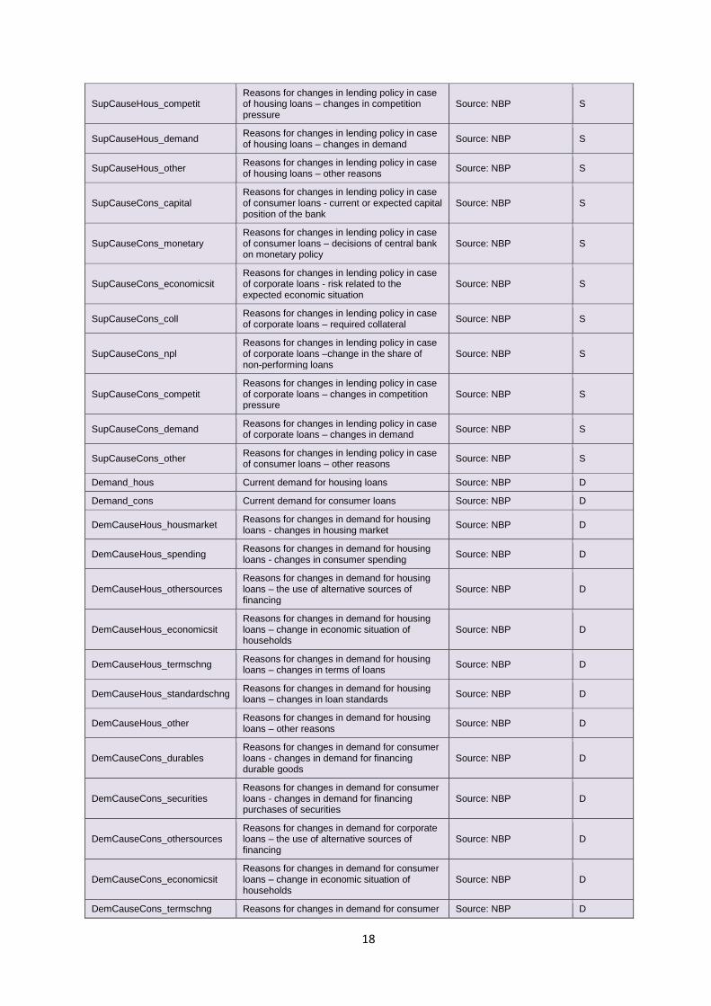
The full list of variables (survey, banking and macro indicators) used in the research was
included in Table 1.
5. Results
5.1.Aggregate approach
The selection of variables to final specifications in disequilibrium model was made according
to following steps. Very broad list of potential regressors (see Table 1) was narrowed using
the t-test of Pearson coefficient of correlation. Not only coincident, but also lagged relations
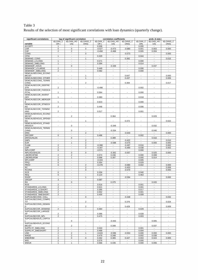
were taken into account. The results of selection are presented in Table 3 and the conclusions
are as follows:
a) In case of corporate segment the list of significant variables was relatively long
comparing to housing and consumer segment.
b) Most significant correlations the corporate credit growth had with such demand-side
variables as questions from SLOS concerning current and forecasted demand of SMEs and
large companies for long term loans, questions about reasons of demand change like fixed
capital needs, inventories, mergers funding, change of loan standards and terms. Other
significant demand factors are, amongst others, percentage of requested loans, consumer and
production prices, GDP growth, Polish stock market index, return on sales.
8
c) The strongest supply-side relations in case of corporates had questions about current
standards for all types of loans (both short and long-term), questions concerning supply
causes such as demand and credit risk reasons (also large exposures) and forecasts of supply
for loans for SME. Indicators of capital adequacy, funding abilities and credit risk in banking
system also passed the test as expected.
d) Interest rate changes also were significant. Both national loan interest rates: interbank
– WIBOR and corporate– RCR had strongest coincident relation and foreign interest rates
influenced loans with two-quarter time lag.
e) The strongest determinants of housing loans from the tested list were economic
situation, change of standards and terms of loans, wages, consumer confidence indicator,
foreign exchange rate, interest rates.
f) Change of consumer loans was significantly correlated with economic situation of
households, consumption, GDP, change of terms of loans, change of incomes, employment,
capital adequacy ratio, foreign funding, funding gap, provisions to loans to households,
competition on the market and interest rates.
Next, the selected variables were divided into two groups – demand and supply side. Simple
linear regressions of demand and supply were tested, were demand and supply were
represented by observable credit change. Tests of significance, colinearity check enabled to
select final set of variables (regressors). These are:
1a. demand for corporate loans - net percent of the answers from the survey about reasons for
the change in demand: DEMCAUSECOR_DEBTRESTR(-2),
DEMCAUSECOR_MERGERS(-1), DEMCAUSECOR_TERMSCHNG(-2), and consumer
prices CPIQ(-1), change of interest rate D(RCR), stock market index WIG(-2), index of
consumer sentiment - CSI(-1), government support for SMEs - MINIMIS.
1b. supply of corporate loans – capital adequacy ratio CAR, change of deposit rate for
corporates D(DRCORP), foreign funding FLIAB(-2), non-performing loans ratio
INPLCORP, provisions to loans ratio PROV, change of loan interest rate for corporates
D(RCR), net percent of answers from the survey concerning credit standards for large
companies, of short-term loans STANDARDS_LCSHORT(-2), forecast of supply of loans for
SMEs SUPPLYF_SMELONG(-2), and government support for SMEs - MINIMIS
2a. demand for housing loans –net percent of answers from the survey concerning forecasts of
demand DEMANDF_HOUS, reasons of demand changes
DEMCAUSEHOUS_STANDARDSCH, and other variables, such as change of LIBOR or FX
9
rate D(LIBORCHF3M), CHF(-2), change of loan interest rate D(RH), consumer sentiment
indicator CSI(-1).
2b. supply of housing loans – net percent of answers from the survey concerning reasons of
change in supply SUPCAUSEHOUS_ECONOMICSIT(-2), CAR, change of deposit rate for
households D(DRHOUHLDS), non-performing loan ratio INPLHOUSHLDS, change of
interest rate of zloty and CHF housing loans D(RH), D(LIBORCHF3M), and introducing
government programme GOVP.
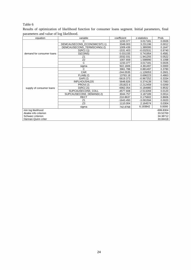
3a. demand for consumer loans – net percent of answers from the survey concerning reasons
of change in demand DEMCAUSECONS_ECONOMICSIT(-1),
DEMCAUSECONS_TERMSCHNG(-2), change in interest rate of consumer loans D(RC(-
1)), change in overall consumption D(CONS) and seasonal factors (Z).
3b. supply of consumer loans – capital adequacy ratio CAR, foreign funding FLIAB(-2),
funding gap GAP(-2), ratio of non-performing loans for households INPLHOUSHLDS,
provisions to loans PROV(-2), change of interest rate of consumer loans D(RC(-2)), causes of
supply according to survey such as collateral SUPCAUSECONS_COLL and demand
SUPCAUSECONS_DEMAND(-2), recommendation of Polish FSA (RECT) and seasonal
factors (Z).
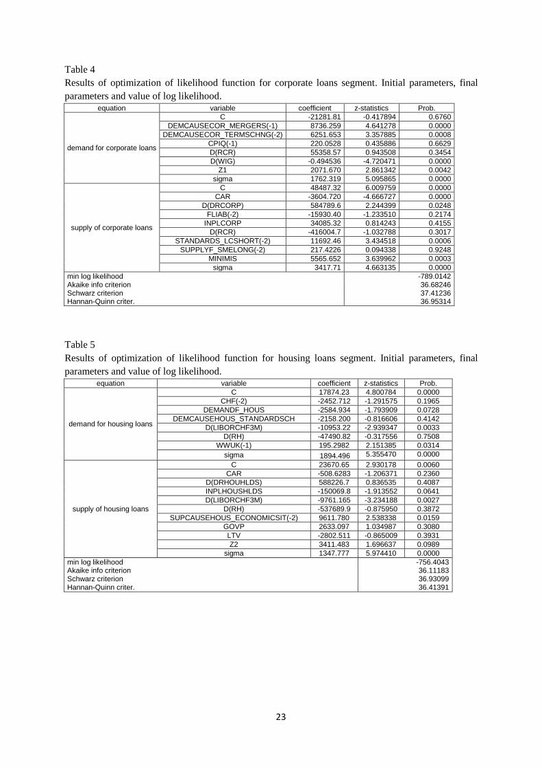
Final specifications of regressors for each loan segment were put into disequilibrium model in
the form (1)3. Firstly, initial parameters were obtained using OLS method and then nonlinear
optimization of regime-switching model was made with the use of the Broyden-Fletcher-
Goldfarb-Shanno (BFGS) algorithm which is one of the quasi-Newton methods of optimizing.
Vectors of initial and optimal parameters are included in Table 4, 5 and 6 together with
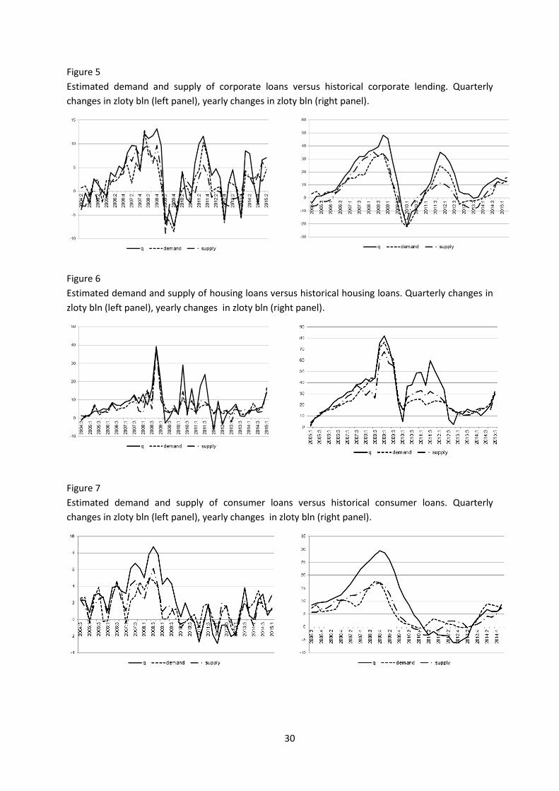
significance tests. At Figure 5, 6 and 7 quarterly changes of estimated demand and supply are
given together with historical values of observable credit changes. Figure 8, 9, 10 includes
probabilities of supply and demand regimes estimated for particular periods.
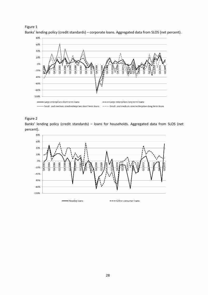
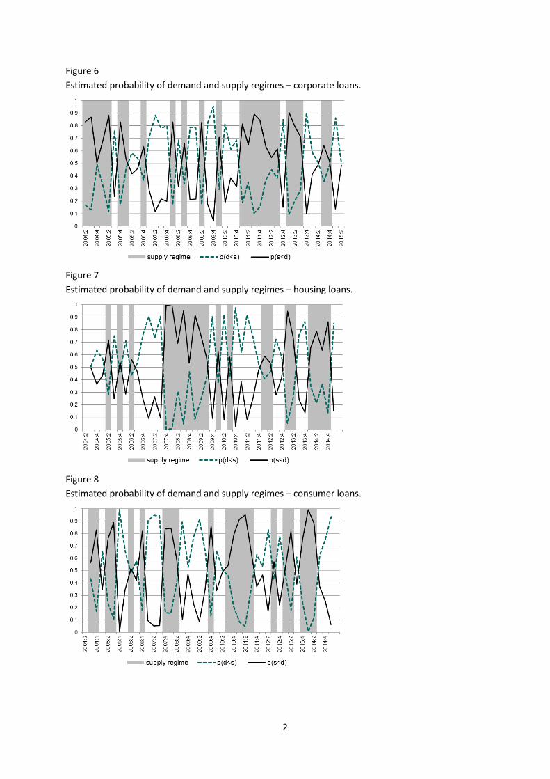
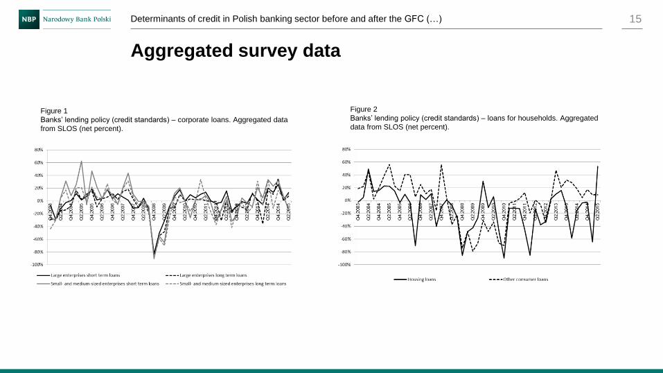
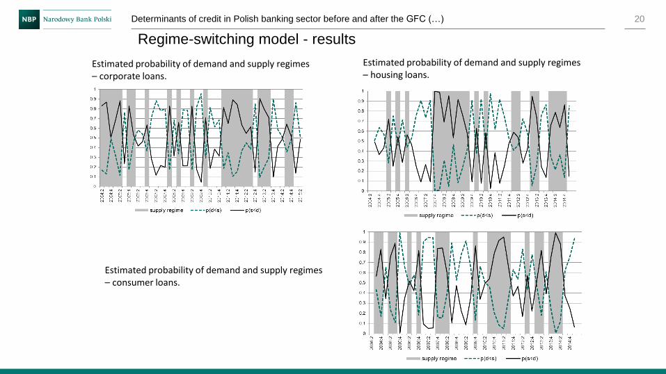
In case of corporate loans, from 2004 to 2008 banks were easing credit policy (see Figure 1).
That time banks also declared relatively high demand for loans from enterprises (and Figure
3). The results of estimation suggest that at the beginning of this period demand was slightly
higher than supply and just before the Crisis tendency has reversed. It means that at that
second period easier credit standards, increasing supply of credit did meet the financial needs
3 However to simplify the analysis, we assume 𝜎12 = 0.
10
of corporates. In 2009 banks curbed supply of loans, however the results suggest that such
deep drop of credit dynamics to negative values was driven more by decreasing demand.
Early after the crisis, in 2011, the demand was increasing faster than supply, as financial
needs connected with infrastructure investments of football competition Euro 2012
quickened. Supply did not increase much, and even went down in the second half of 2012 as
banks tightened credit policy due to worsening quality of loans of enterprises involved in
infrastructure projects connected with Euro 2012. Increasing prices of materials raised the real
costs comparing to agreed contracts which led large infrastructure companies to financial
problems. From 2014 the supply of credit to corporates increased faster than demand showing
rather reluctance of firms towards taking a loan.
In case of housing credit to households, results suggests that until 2007 demand and supply
were more or less in equilibrium. However before the lending crisis supply regime started to
dominate. The second period of disequilibrium was just after the Crisis, till 2012, where
demand was lower than supply (see Figure 6).
Consumer loan segment before the Crisis was more demand-regime dominated and after the
Crisis supply regime was more frequent (Figure 7).
5.2.Bank-level approach
Bank-level approach focuses on the analysis of the influence of particular demand and supply
variables on the credit dynamics before and after the last financial crisis.
For each segment of loans two specifications were tested in two subsamples. First
specification is basing on results included in Wośko (2015), where statistically and
predictively best specifications of panel models of credit growth in Poland were found.
Equations include both, demand and supply variables. Second specification uses in the role of
regressors the data gathered only from SLOS on disaggregated level. These are answers
concerning credit policy (credit standards) and demand for loans.
According to Polish characteristics of the consequences of world financial crisis, the timeline
was divided into periods “before the Crisis”, it means to the end of 2008, and “after the
Crisis”, which starts from 2011. Both panel equations were estimated on these two
subsamples. Tables from 7 to 12 include the results of estimations.
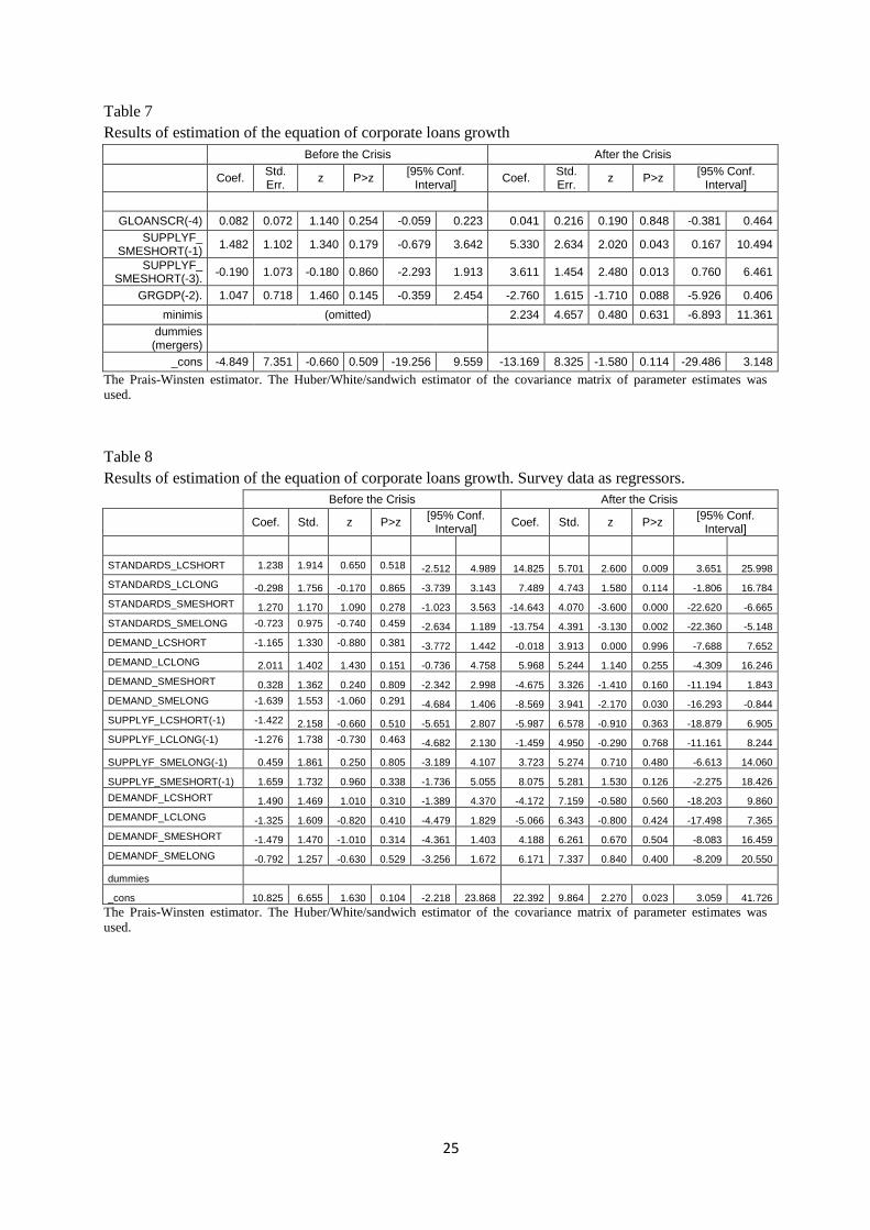
According to Wośko (2015), the growth of corporate loans in Poland depends strongly on past
developments in this category, banks’ policy expectations from the last quarter, past GDP rate
of growth, and from 2014 onwards – the government guarantee programme for SMEs. In case
11
of corporate segment, as the first specification, similar equation was estimated (see Table 7).
The second equation includes only answers from the survey regarding large and SMEs and
concerning short and long term loans (Table 8).
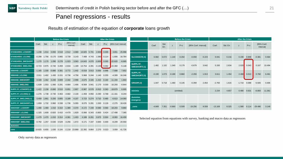
Estimations of both specifications in two subsamples suggest the strong rise of significance of
supply factors of credit in the period after the Crisis.
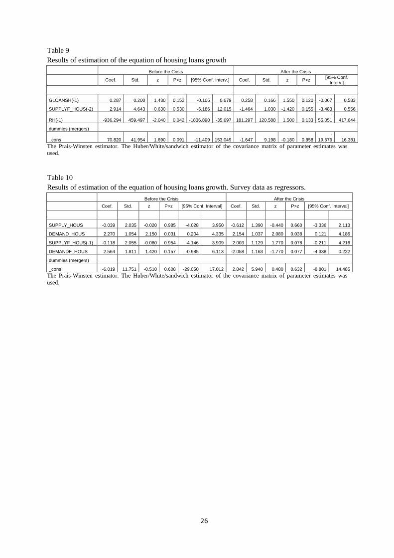
In case of segment of housing loans, the conclusions are quite similar to corporate, however
the rise in significance of supply factors is smaller. But in fact, in the period after the Crisis,
answers on the questions concerning supply had higher values of the test of significance (see
Table 9 and 10).
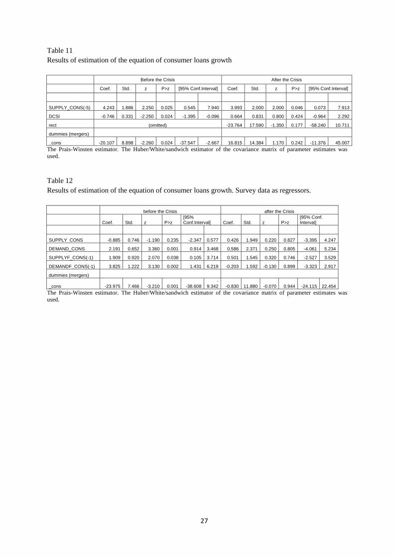
The growth of consumer loans depends on past banks’ policy and on the last-quarter change
of consumer sentiment indicator (see Table 11). Consumer loans are the short-term financing
of consumer goods, these are loans at current accounts, credit card accounts, etc. The higher
the optimism concerning the following months, the more prominent the rise of household
expenses, as households predict that their credibility will improve.
Estimation of growth of consumer loans in two subsamples of both equations has shown
decrease of information value of both demand and supply factors in the second subsample
(Table 11 and 12). In other words, significance of demand as well as supply factors decreased
after the Crisis.
6. Conclusions
This paper described the influence of demand and supply determinants on the credit
growth in the sector of commercial banks in Poland. The main idea of the concept was to use
survey information in the form of panel data from Senior Loan Officers Opinion Survey
(SLOS). The main objective of included models was answer about possible changes in
tendencies of the influence of demand and supply factors as the result of the last financial
crisis at the disaggregated (for particular banks, different types of loans) and aggregated (the
commercial banks’ sector) level.
Two methodological approaches were used. First one, on aggregated data, was time series
regression with the use of disequilibrium econometric approach (regime-switching model)
and the second one was a panel regression on disaggregated (bank level) data.
The results received on the bank-level data suggest increasing significance of supply factors
after the Crisis in case of corporate and housing loans. Results on aggregated data with the

12
use of regime-switching model confirm these results in case of corporate loan segment.
However disequilibrium (aggregated approach) suggest also increase of probability of supply
side in consumer loans in the period following GFC.
13
References
Artus (1984), Le fonctionnement du marché du crédit: diverses analyses dans un cadre de
déséquilibre, Revue économique. Vol. 35, no 4, pp. 591-622.
Asea P.K., Blomberg S.B. (1997), Lending cycles, Journal of Econometrics, 83.1-2: p. 89-
128.
Balke N.S., Zeng Z. (2013), Credit Demand, Credit Supply, and Economic Activity, The B.E.
Journal of Macroeconomics, De Gruyter, vol. 13(1), pages 38, October.
Brown M., Kirschenmann K., Ongena S. (2010), Foreign Currency loans – demand or supply
driven?, Proceedings of the German Development Economics Conference, Hannover 2010,
No.8.
Burdeau E. (2014), Assessing dynamics of credit supply and demand for French SMEs, an
estimation based on the Bank Lending Survey, Seventh IFC Conference on “Indicators to
support Monetary and Financial Stability Analysis: Data Sources and Statistical
Methodologies” held at the BIS in Basel on 4 and 5 September 2014.
Calza, A., M. Manrique and J. Souza (2006), Aggregate Loans to the Euro Area Private
Sector, Quarterly Review of Economics and Finance, Vol. 46, pp. 2211-26.
Del Giovane P., Eramo G., Nobili A. (2010), Disentangling demand and supply in credit
developments: a survey-based analysis for Italy, Banca d’Italia Working Papers, No 764.
Ghosh S.R., Ghosh A.R. (2000), East Asia in the aftermath: Was there a crunch?, Deutsche
Bank Research, Research notes in economics and statistics, No. 00-5.
Ito T., Ueda K. (1981), Tests of the equilibrium hypothesis in disequilibrium econometrics: an
international comparison of credit rationing, International Economic Review, Vol. 22
(October), pp 691-708.
Kakes, J. (2000), Identifying the Mechanism: Is There a Bank Lending Channel of Monetary
Transmission in the Netherlands?, Applied Economics, Vol. 7, pp. 63-7.
Kierzenkowski R., Hurlin C. (2002), A theoretical and empirical assessment of the bank
lending channel and loan market disequilibrium in Poland, Materiały i Studia, NBP.
Laffont J., Garcia R. (1977), Disequilibrium econometrics for business loans, Econometrica,
Vol. 45 (July), pp 1187-1204.
Lagarias, J. C., Reeds J. A., Wright M. H., Wright P. E. (1998), Convergence Properties of
the Nelder-Mead Simplex Method in Low Dimensions., SIAM Journal of Optimization, Vol.
9, Number 1, pp. 112–147.
Łyziak T., Kapuściński M., Przystupa J., Stanisławska E., Sznajderska A., Wróbel E. (2014),
Mechanizm transmisji polityki pieniężnej w Polsce. Co wiemy w 2013 roku?, Materiały i
Studia nr 306, NBP.
14
Martin C. (1990), Corporate borrowing and credit constraints: structural disequilibrium
estimates for the U.K., The Review of Economics and Statistics, The MIT Press.
Mello L., Pisu M. (2009), The Bank Lending Channel of Monetary Transmission in Brazil. A
VECM approach, OECD Economics Department Working Papers No. 711.
Pazarbasioglu C. (1997), A Credit Crunch ? Finland in the Aftermath of the Banking Crisis,
IMF Staff Papers, Vol. 44, N◦3, September, pp. 315-327.
Sealy (1979), Credit Rationing in the Commercial Loan Market: Estimates of a Structural
Model Under Conditions of Disequilibrium, The Journal of Finance, Vol. 34, Issue 3, pp 689–
702.
Spencer P.D. (1975), A disequilibrium model of personal sector bank advances. 1964-1974:
Some preliminary results, Working Paper, HM Treasury.
Stenius M. (1983), Testing the Efficiency of the Finnish Bond Market, The Finnish Journal of
Business Economics (Jan. 1983), 19-29.
Wośko Z. (2015), Modelling Credit Growth in Commercial Banks with the Use of Data from
Senior Loan Officers Opinion Survey, NBP Working Papers, No 210.
Financial Stability Report. July 2010., National Bank of Poland.
http://www.nbp.pl/homen.aspx?f=/en/systemfinansowy/stabilnosc.html
15
Table 1
Variables tested in the models of supply and demand and their transformations (in parentheses).
abbreviation description details supply/ demand side
(D)CSI consumer sentiment indicator (quarter-to-quarter change)
Source: Polish Central Statistical Office
D
(G)RGDP gross domestic product (rate of growth, constant prices)
Source: Polish Central Statistical Office
D
(G)WIG Warsaw Stock Exchange Index (rate of change)
Source: Reuters D
CHF/PLN, EUR/PLN, USD/PLN exchange rates Source: NBP D,S
(R)CONS consumption (constant prices) Source: Polish Central Statistical Office
D
CPI consumer products inflation (q/q) Source: Polish Central Statistical Office
D
ECI business climate indicator Source: Polish Central Statistical Office
D
SPI sold production of industry (q/q) Source: Polish Central Statistical Office
D
PPI production prices of industry Source: Polish Central Statistical Office
D
(D)EMPL number of employed in the corporate sector Source: Polish Central Statistical Office
D
INC households' disposable income Source: Polish Central Statistical Office
D
HHP Housing prices q/q Source: NBP D
ROE,ROA,ROS profitability ratios of corporates Source: Polish Central Statistical Office
D
U unemployment rate Source: Polish Central Statistical Office
D
WAGE average wage Source: Polish Central Statistical Office
D
(D)WIBOR3M, (D)LIBORCHF3M, (D)LIBOREUR3M
interbank interest rates Source: NBP, Reuters D,S
(D)DRH deposit interest rate - households Source: NBP S
(D)DRC deposit interest rate - corporates Source: NBP S
(D)FGAP
Funding gap - the difference between the sum of loans to non-financial sector and government and the sum of deposits from these sectors as a percentage of loans.
Source: NBP S
(D)IBGAP
total interbank loans of the bank minus its total interbank borrowings, as fraction of bank's assets (quarter-to-quarter change)
Source: NBP S
(G)LOANSC consumer loans (quarter-to-quarter growth) Source: NBP regressand
(G)LOANSCR corporate loans (quarter-to-quarter growth, constant prices)
Source: NBP regressand
(G)LOANSH housing loans (quarter-to-quarter growth, constant prices)
Source: NBP regressand
CAR capital adequacy ratio Source: NBP S
FLIAB liabilities from foreign financial institutions to total assets
Source: NBP S
govp Binary variable. Government support plan for families buying their first flat (“Rodzina na
Source: own computations
S
16
swoim”)
minimis Binary variable. Government support for SMEs in the form of loans guarantee plan. (“1” from 2013, “0” otherwise)
Source: own computations
S
(D)NPLHoushlds non-performing loans – loans from households Source: NBP S
INPLHoushlds non-performing loans ratio – loans from households
Source: NBP S
(D)NPLcons non-performing loans - consumer loans Source: NBP S
(D)NPLcorp non-performing loans - corporate loans Source: NBP S
(D)NPLhousing non-performing loans - housing loans Source: NBP S
INPLcons non-performing loans ratio - consumer loans Source: NBP S
INPLcorp non-performing loans ratio - corporate loans Source: NBP S
INPLhousing non-performing loans ratio - housing loans Source: NBP S
PROV provisions to loans, annualized data Source: NBP S
(D)RC interest rate – consumer loans Source: NBP D,S
(D)RCR interest rate – corporate loans Source: NBP D,S
rect
Binary variable (“1” from second half of 2013, “0” otherwise). Adjustment to Recommendation T of the Polish Financial Authority which eased the standards of consumer loans
Source: own computations
S
(D)RH interest rate – housing loans Source: NBP D,S
req percentage of enterprises applying for credit - survey data
Source: NBP D
accept the share of approved loan applications - survey data
Source: NBP
Standards_LCShort current credit policy (credit standards) concerning short-term loans to large companies
Source: NBP S
Standards_LCLong current credit policy (credit standards) concerning longterm loans to large companies
Source: NBP S
Standards_SMEShort current credit policy (credit standards) concerning short-term loans to SMEs
Source: NBP S
Standards_SMELong current credit policy (credit standards) concerning long-term loans to SMEs
Source: NBP S
SupCauseCor_capital Reasons for changes in lending policy - current or expected capital position of the bank
Source: NBP S
SupCauseCor_monetary Reasons for changes in lending policy – decisions of central bank on monetary policy
Source: NBP S
SupCauseCor_economicsit Reasons for changes in lending policy - risk related to the expected economic situation
Source: NBP S
SupCauseCor_industryrisk Reasons for changes in lending policy – industry risk
Source: NBP S
SupCauseCor_largeexp Reasons for changes in lending policy – risk related to large borrowers
Source: NBP S
SupCauseCor_npl Reasons for changes in lending policy – change in the share of non-performing loans
Source: NBP S
SupCauseCor_competit Reasons for changes in lending policy – changes in competition pressure
Source: NBP S
SupCauseCor_demand Reasons for changes in lending policy – change in demand for corporate loans
Source: NBP S
SupCauseCor_other Reasons for changes in lending policy – other reasons
Source: NBP S
Demand_LCShort Demand for loans – short term loans for large companies
Source: NBP D
17
Demand_LCLong Demand for loans – long term loans for large companies
Source: NBP D
Demand_SMEshort Demand for loans – short term loans for SMEs Source: NBP D
Demand_SMElong Demand for loans – long term loans for SMEs Source: NBP D
DemCauseCor_fixedcapital Reasons for changes in demand for corporate loans - changes in demand for financing fixed assets (investments)
Source: NBP D
DemCauseCor_inventory Reasons for changes in demand for corporate loans - changes in financing needs for inventories and working capital
Source: NBP D
DemCauseCor_mergers Reasons for changes in demand for corporate loans - changes in demand for financing mergers and acquisitions
Source: NBP D
DemCauseCor_debtrestr Reasons for changes in demand for corporate loans - changes in demand for financing debt restructuring
Source: NBP D
DemCauseCor_othersources Reasons for changes in demand for corporate loans - the use of alternative sources of financing
Source: NBP D
DemCauseCor_termschng Reasons for changes in demand for corporate loans - change of corporate loans terms
Source: NBP D
DemCauseCor_stndchng Reasons for changes in demand for corporate loans – change of corporate loans standards
Source: NBP D
DemCauseCor_other Reasons for changes in demand for corporate loans – other reasons
Source: NBP D
SupplyF_LCShort Foreseen supply of short term loans for large companies
Source: NBP D
SupplyF_LClong Foreseen supply of long term loans for large companies
Source: NBP S
SupplyF_SMEshort Foreseen supply of short term loans for SMEs Source: NBP S
SupplyF_SMElong Foreseen supply of long term loans for SMEs Source: NBP S
DemandF_LCShort Foreseen demand for loans – short term loans for large companies
Source: NBP D
DemandF_LCLong Foreseen demand for loans – long term loans for large companies
Source: NBP D
DemandF_SMEshort Foreseen demand for loans – short term loans for SMEs
Source: NBP D
DemandF_SMElong Foreseen demand for loans – long term loans for SMEs
Source: NBP D
Standards_hous current credit policy (credit standards) concerning housing loans
Source: NBP S
Standards_cons current credit policy (credit standards) concerning consumer loans
Source: NBP S
SupCauseHous_capital Reasons for changes in lending policy in case of housing loans - current or expected capital position of the bank
Source: NBP S
SupCauseHous_monetary Reasons for changes in lending policy in case of housing loans – decisions of central bank on monetary policy
Source: NBP S
SupCauseHous_economicsit Reasons for changes in lending policy in case of housing loans - risk related to the expected economic situation
Source: NBP S
SupCauseHous_marketsit Reasons for changes in lending policy in case of housing loans – housing market situation
Source: NBP S
SupCauseHous_npl Reasons for changes in lending policy in case of housing loans –change in the share of non-performing loans
Source: NBP S
18
SupCauseHous_competit Reasons for changes in lending policy in case of housing loans – changes in competition pressure
Source: NBP S
SupCauseHous_demand Reasons for changes in lending policy in case of housing loans – changes in demand
Source: NBP S
SupCauseHous_other Reasons for changes in lending policy in case of housing loans – other reasons
Source: NBP S
SupCauseCons_capital Reasons for changes in lending policy in case of consumer loans - current or expected capital position of the bank
Source: NBP S
SupCauseCons_monetary Reasons for changes in lending policy in case of consumer loans – decisions of central bank on monetary policy
Source: NBP S
SupCauseCons_economicsit Reasons for changes in lending policy in case of corporate loans - risk related to the expected economic situation
Source: NBP S
SupCauseCons_coll Reasons for changes in lending policy in case of corporate loans – required collateral
Source: NBP S
SupCauseCons_npl Reasons for changes in lending policy in case of corporate loans –change in the share of non-performing loans
Source: NBP S
SupCauseCons_competit Reasons for changes in lending policy in case of corporate loans – changes in competition pressure
Source: NBP S
SupCauseCons_demand Reasons for changes in lending policy in case of corporate loans – changes in demand
Source: NBP S
SupCauseCons_other Reasons for changes in lending policy in case of consumer loans – other reasons
Source: NBP S
Demand_hous Current demand for housing loans Source: NBP D
Demand_cons Current demand for consumer loans Source: NBP D
DemCauseHous_housmarket Reasons for changes in demand for housing loans - changes in housing market
Source: NBP D
DemCauseHous_spending Reasons for changes in demand for housing loans - changes in consumer spending
Source: NBP D
DemCauseHous_othersources Reasons for changes in demand for housing loans – the use of alternative sources of financing
Source: NBP D
DemCauseHous_economicsit Reasons for changes in demand for housing loans – change in economic situation of households
Source: NBP D
DemCauseHous_termschng Reasons for changes in demand for housing loans – changes in terms of loans
Source: NBP D
DemCauseHous_standardschng Reasons for changes in demand for housing loans – changes in loan standards
Source: NBP D
DemCauseHous_other Reasons for changes in demand for housing loans – other reasons
Source: NBP D
DemCauseCons_durables Reasons for changes in demand for consumer loans - changes in demand for financing durable goods
Source: NBP D
DemCauseCons_securities Reasons for changes in demand for consumer loans - changes in demand for financing purchases of securities
Source: NBP D
DemCauseCons_othersources Reasons for changes in demand for corporate loans – the use of alternative sources of financing
Source: NBP D
DemCauseCons_economicsit Reasons for changes in demand for consumer loans – change in economic situation of households
Source: NBP D
DemCauseCons_termschng Reasons for changes in demand for consumer Source: NBP D

19
loans – changes in terms of loans
DemCauseCons_standardschng Reasons for changes in demand for consumer loans – changes in loan standards
Source: NBP D
DemCauseCons_other Reasons for changes in demand for consumer loans – other reasons
Source: NBP D
SupplyF_hous Foreseen supply of housing loans Source: NBP S
SupplyF_cons Foreseen supply of consumer loans Source: NBP S
DemandF_hous Foreseen demand for housing loans Source: NBP D
DemandF_cons Foreseen demand for consumer loans Source: NBP D
(G)- growth rate, (D) – first difference, (R)- constant prices, (Z1, Z2,….) – seasonal factors
20
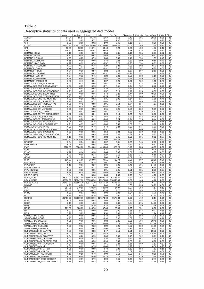
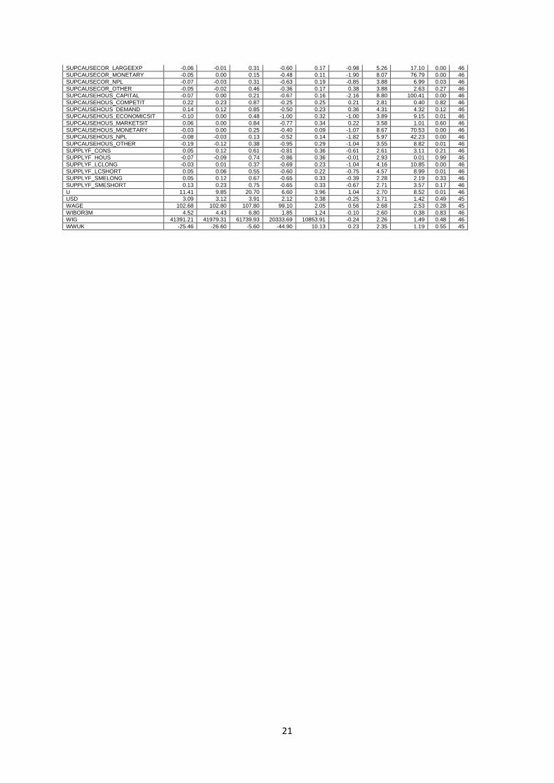
Table 2
Descriptive statistics of data used in aggregated data model Mean Median Max Min Std.Dev. Skewness Kurtosis Jarque-Bera Prob. Obs.
ACCEPT 84.34 85.84 91.70 66.67 5.52 -1.43 5.01 20.78 0.00 41
CAR 13.76 13.95 15.77 10.88 1.37 -0.53 2.31 3.03 0.22 45
CHF 2.93 2.95 3.62 2.09 0.46 -0.18 1.74 3.20 0.20 45
CONS 202413.70 202617.20 268262.00 138134.00 39639.42 -0.01 1.65 3.49 0.17 46
CPI 98.39 98.85 110.71 83.48 9.29 0.00 1.50 4.32 0.12 46
CPIQ 100.61 100.50 102.07 99.46 0.70 0.28 2.15 1.99 0.37 46
DEMAND_CONS 0.13 0.16 0.67 -0.54 0.31 -0.15 2.35 0.97 0.62 46
DEMAND_HOUS 0.13 0.15 0.97 -0.69 0.42 0.13 2.33 0.97 0.61 46
DEMAND_LCLONG 0.23 0.25 0.79 -0.60 0.33 -0.41 2.59 1.59 0.45 46
DEMAND_LCSHORT 0.18 0.19 0.60 -0.46 0.23 -0.30 3.00 0.68 0.71 46
DEMAND_SMELONG 0.19 0.19 0.70 -0.52 0.28 -0.23 2.54 0.81 0.67 46
DEMAND_SMESHORT 0.22 0.21 0.76 -0.29 0.22 0.30 3.02 0.71 0.70 46
DEMANDF_CONS 0.44 0.53 0.87 -0.32 0.30 -0.79 2.87 4.82 0.09 46
DEMANDF_HOUS 0.24 0.30 0.97 -0.83 0.42 -0.57 3.07 2.51 0.29 46
DEMANDF_LCLARGE 0.33 0.38 0.85 -0.31 0.32 -0.22 1.97 2.41 0.30 46
DEMANDF_LCSHORT 0.34 0.32 0.75 -0.20 0.23 -0.20 2.32 1.19 0.55 46
DEMANDF_SMELONG 0.38 0.45 0.93 -0.62 0.38 -0.69 2.89 3.63 0.16 46
DEMANDF_SMESHORT 0.43 0.47 0.91 -0.07 0.25 -0.28 2.29 1.55 0.46 46
DEMCAUSECONS_DURABLES 0.23 0.24 0.96 -0.67 0.43 -0.22 2.28 1.35 0.51 46
DEMCAUSECONS_ECONOMICSIT 0.07 0.03 0.93 -0.71 0.41 0.24 2.62 0.72 0.70 46
DEMCAUSECONS_OTHER 0.09 0.04 0.68 -0.38 0.19 0.61 5.13 11.51 0.00 46
DEMCAUSECONS_OTHERSOURCE -0.11 -0.09 0.32 -0.57 0.19 -0.16 3.25 0.33 0.85 46
DEMCAUSECONS_SECURITIES 0.01 0.00 0.86 -0.74 0.25 0.44 8.00 49.30 0.00 46
DEMCAUSECONS_STANDARDSCH 0.13 0.11 0.73 -0.74 0.33 -0.30 3.03 0.71 0.70 46
DEMCAUSECONS_TERMSCHNG 0.22 0.16 0.82 -0.31 0.31 0.14 2.15 1.55 0.46 46
DEMCAUSECOR_DEBTRESTR 0.12 0.02 0.71 -0.40 0.22 0.66 3.45 3.68 0.16 46
DEMCAUSECOR_FIXEDCAPITAL 0.31 0.42 0.99 -0.91 0.54 -0.74 2.34 4.97 0.08 46
DEMCAUSECOR_INVENTORY 0.35 0.38 1.00 -0.40 0.36 -0.34 2.43 1.53 0.47 46
DEMCAUSECOR_MERGERS 0.06 0.05 0.55 -0.65 0.26 -0.55 4.20 5.09 0.08 46
DEMCAUSECOR_OTHER 0.07 0.02 0.66 -0.61 0.21 0.13 5.70 14.12 0.00 46
DEMCAUSECOR_OTHERSOURCES -0.06 -0.06 0.21 -0.26 0.10 0.05 2.82 0.08 0.96 46
DEMCAUSECOR_STNDCHNG 0.03 0.01 0.32 -0.55 0.18 -0.90 4.42 10.09 0.01 46
DEMCAUSECOR_TERMSCHNG 0.07 0.06 0.62 -0.48 0.24 -0.24 2.95 0.44 0.80 46
DEMCAUSEHOUS_ECONOMICSIT 0.04 0.01 0.76 -0.86 0.38 -0.10 2.65 0.31 0.86 46
DEMCAUSEHOUS_HOUSMARKET 0.21 0.35 0.97 -0.88 0.53 -0.50 2.18 3.20 0.20 46
DEMCAUSEHOUS_OTHER 0.09 0.06 0.78 -0.44 0.24 0.33 3.75 1.91 0.39 46
DEMCAUSEHOUS_OTHERSOURCE -0.04 -0.04 0.59 -0.52 0.22 0.31 4.66 5.99 0.05 46
DEMCAUSEHOUS_SPENDING 0.02 0.00 0.65 -0.54 0.24 0.32 3.30 0.98 0.61 46
DEMCAUSEHOUS_STANDARDSCH 0.01 0.05 0.69 -0.85 0.32 -0.59 4.15 5.22 0.07 46
DEMCAUSEHOUS_TERMSCHNG 0.11 0.08 0.94 -0.83 0.41 -0.09 2.51 0.52 0.77 46
DINC 206843.10 204976.00 283927.00 143316.00 37965.48 0.12 1.84 2.63 0.27 45
DRCORP 0.04 0.04 0.06 0.02 0.01 0.09 2.45 0.63 0.73 45
DRHOUHLDS 0.04 0.04 0.06 0.02 0.01 0.17 2.72 0.37 0.83 45
EMPL 5260.35 5364.00 5549.00 4000.00 322.25 -1.78 6.83 46.85 0.00 41
EUR 4.09 4.11 4.78 3.35 0.31 -0.11 3.31 0.26 0.88 45
FLIAB 0.12 0.14 0.20 0.04 0.05 -0.36 1.56 4.87 0.09 45
GAP -0.01 0.08 0.14 -0.27 0.15 -0.69 1.75 6.58 0.04 46
GOVP 0.52 1.00 1.00 0.00 0.51 -0.09 1.01 7.67 0.02 46
HHP 136.67 141.86 158.68 90.11 16.74 -1.30 4.09 12.98 0.00 39
INPLCONS 0.13 0.12 0.18 0.07 0.04 0.16 1.59 4.00 0.14 46
INPLCORP 0.12 0.11 0.27 0.06 0.05 1.49 5.01 24.70 0.00 46
INPLHOUSHLDS 0.07 0.07 0.13 0.04 0.02 1.05 5.07 16.75 0.00 46
INPLHOUSING 0.03 0.03 0.05 0.01 0.01 0.51 2.85 2.01 0.37 46
LIBORCHF3M 0.74 0.25 2.96 -0.69 0.99 1.19 3.04 10.82 0.00 46
LIBOREUR3M 1.84 1.53 5.28 0.03 1.55 0.73 2.42 4.73 0.09 46
LOAN_COR 193007.20 206927.00 266684.10 116001.70 52782.87 -0.27 1.55 4.61 0.10 46
LOAN_HOUS 193876.60 210647.90 365036.50 29575.83 118043.40 -0.09 1.43 4.78 0.09 46
LOANS_CONS 103412.20 126887.70 138741.20 41875.23 36646.45 -0.59 1.63 6.27 0.04 46
MINIMIS 0.20 0.00 1.00 0.00 0.40 1.53 3.35 18.29 0.00 46
PPI 387.75 379.98 438.19 326.89 34.97 0.07 1.53 4.17 0.12 46
PPIQ 102.46 102.40 109.57 97.33 3.27 0.37 2.48 1.54 0.46 46
PROV 0.01 0.01 0.02 0.00 0.00 0.34 2.31 1.76 0.41 45
RC 0.15 0.15 0.16 0.09 0.01 -2.01 8.23 81.55 0.00 45
RCONS 199496.20 200569.60 271934.60 137373.60 40576.89 0.03 1.72 3.17 0.21 46
RCR 0.06 0.06 0.08 0.04 0.01 -0.43 2.93 1.40 0.50 45
RECT 0.15 0.00 1.00 0.00 0.36 1.94 4.75 34.63 0.00 46
REQ 24.38 23.89 33.19 16.70 4.63 0.23 1.89 2.46 0.29 41
RGDP 181.03 180.85 240.73 137.66 25.95 0.25 2.51 0.93 0.63 45
RH 0.07 0.07 0.09 0.05 0.01 0.15 2.43 0.77 0.68 45
ROS 5.19 5.23 6.40 4.30 0.60 0.16 2.10 1.74 0.42 46
STANDARDS_CONS 0.00 0.05 0.56 -0.79 0.36 -0.62 2.58 3.25 0.20 46
STANDARDS_HOUS -0.15 -0.08 0.49 -0.90 0.32 -0.69 2.93 3.69 0.16 46
STANDARDS_LCLONG -0.06 0.00 0.35 -0.82 0.21 -1.39 5.86 30.45 0.00 46
STANDARDS_LCSHORT -0.01 0.02 0.26 -0.83 0.19 -2.24 10.01 132.74 0.00 46
STANDARDS_SMELONG -0.05 -0.02 0.33 -0.89 0.26 -1.02 4.38 11.58 0.00 46
STANDARDS_SMESHORT 0.01 0.04 0.63 -0.90 0.28 -0.81 4.66 10.37 0.01 46
SUPCAUSECONS_CAPITAL 0.01 0.00 0.52 -0.47 0.16 0.81 6.66 30.73 0.00 46
SUPCAUSECONS_COLL -0.03 0.00 0.17 -0.44 0.11 -2.39 9.22 118.15 0.00 46
SUPCAUSECONS_COMPETIT 0.34 0.26 0.95 -0.08 0.30 0.49 2.02 3.71 0.16 46
SUPCAUSECONS_DEMAND 0.20 0.10 0.73 -0.20 0.23 0.77 2.51 4.99 0.08 46
SUPCAUSECONS_ECONOMICSIT -0.06 0.00 0.54 -0.90 0.30 -0.83 3.91 6.90 0.03 46
SUPCAUSECONS_MONETARY -0.04 0.00 0.56 -0.51 0.23 -0.16 3.69 1.12 0.57 46
SUPCAUSECONS_NPL 0.00 0.02 0.55 -0.66 0.26 -0.27 3.12 0.58 0.75 46
SUPCAUSECONS_OTHER -0.05 0.00 0.69 -0.79 0.26 -0.12 4.53 4.62 0.10 46
SUPCAUSECOR_CAPITAL -0.05 0.00 0.41 -0.90 0.26 -1.09 4.87 15.91 0.00 46
SUPCAUSECOR_COMPETIT 0.18 0.19 0.49 -0.09 0.13 0.03 2.45 0.58 0.75 46
SUPCAUSECOR_DEMAND 0.08 0.08 0.50 -0.23 0.15 0.52 3.79 3.28 0.19 46
SUPCAUSECOR_ECONOMICSIT -0.05 0.07 0.79 -0.99 0.45 -0.47 2.39 2.41 0.30 46
SUPCAUSECOR_INDUSTRYRISK -0.16 -0.08 0.42 -0.75 0.25 -0.56 2.93 2.39 0.30 46
21
SUPCAUSECOR_LARGEEXP -0.06 -0.01 0.31 -0.60 0.17 -0.98 5.26 17.10 0.00 46
SUPCAUSECOR_MONETARY -0.05 0.00 0.15 -0.48 0.11 -1.90 8.07 76.79 0.00 46
SUPCAUSECOR_NPL -0.07 -0.03 0.31 -0.63 0.19 -0.85 3.88 6.99 0.03 46
SUPCAUSECOR_OTHER -0.05 -0.02 0.46 -0.36 0.17 0.38 3.88 2.63 0.27 46
SUPCAUSEHOUS_CAPITAL -0.07 0.00 0.21 -0.67 0.16 -2.16 8.80 100.41 0.00 46
SUPCAUSEHOUS_COMPETIT 0.22 0.23 0.87 -0.25 0.25 0.21 2.81 0.40 0.82 46
SUPCAUSEHOUS_DEMAND 0.14 0.12 0.85 -0.50 0.23 0.36 4.31 4.32 0.12 46
SUPCAUSEHOUS_ECONOMICSIT -0.10 0.00 0.48 -1.00 0.32 -1.00 3.89 9.15 0.01 46
SUPCAUSEHOUS_MARKETSIT 0.06 0.00 0.84 -0.77 0.34 0.22 3.58 1.01 0.60 46
SUPCAUSEHOUS_MONETARY -0.03 0.00 0.25 -0.40 0.09 -1.07 8.67 70.53 0.00 46
SUPCAUSEHOUS_NPL -0.08 -0.03 0.13 -0.52 0.14 -1.82 5.97 42.23 0.00 46
SUPCAUSEHOUS_OTHER -0.19 -0.12 0.38 -0.95 0.29 -1.04 3.55 8.82 0.01 46
SUPPLYF_CONS 0.05 0.12 0.61 -0.81 0.36 -0.61 2.61 3.11 0.21 46
SUPPLYF_HOUS -0.07 -0.09 0.74 -0.86 0.36 -0.01 2.93 0.01 0.99 46
SUPPLYF_LCLONG -0.03 0.01 0.37 -0.69 0.23 -1.04 4.16 10.85 0.00 46
SUPPLYF_LCSHORT 0.05 0.06 0.55 -0.60 0.22 -0.75 4.57 8.99 0.01 46
SUPPLYF_SMELONG 0.05 0.12 0.67 -0.65 0.33 -0.39 2.28 2.19 0.33 46
SUPPLYF_SMESHORT 0.13 0.23 0.75 -0.65 0.33 -0.67 2.71 3.57 0.17 46
U 11.41 9.85 20.70 6.60 3.96 1.04 2.70 8.52 0.01 46
USD 3.09 3.12 3.91 2.12 0.38 -0.25 3.71 1.42 0.49 45
WAGE 102.68 102.80 107.80 99.10 2.05 0.56 2.68 2.53 0.28 45
WIBOR3M 4.52 4.43 6.80 1.85 1.24 -0.10 2.60 0.38 0.83 46
WIG 41391.21 41979.31 61739.93 20333.69 10853.91 -0.24 2.26 1.49 0.48 46
WWUK -25.46 -26.60 -5.60 -44.90 10.13 0.23 2.35 1.19 0.55 45
22
Table 3
Results of the selection of most significant correlations with loan dynamics (quarterly change).
significant correlations lag of significant correlation correlation coefficients prob. (t-stat.)
variable d(LOAN_C
OR ) d(LOAN_HO
US) d(LOANS_C
ONS) d(LOAN_C
OR ) d(LOAN_HO
US) d(LOANS_C
ONS) d(LOAN_C
OR) d(LOAN_HO
US) d(LOANS_C
ONS)
ACCEPT 1 - - 0.558 - - 0.000 - -
CAR 0 0 0 -0.527 -0.473 -0.680 0.001 0.003 0.000
CHF 2 2 - -0.458 -0.468 - 0.005 0.004 -
CONS - - 0 - - -0.573 - - 0.000
CPIQ 1 - - 0.329 - - 0.044 - -
DEMAND_CONS - - 1 - - 0.392 - - 0.015
DEMAND_LCLONG 1 - - 0.571 - - 0.000 - -
DEMAND_SMELONG 1 - - 0.394 - - 0.014 - -
DEMANDF_HOUS - 0 - - -0.339 - - 0.037 -
DEMANDF_LCLARGE 2 - - 0.449 - - 0.006 - -
DEMANDF_SMELONG 2 - - 0.582 - - 0.000 - -
DEMCAUSECONS_ECONOMICSIT - - 1 - - 0.647 - - 0.000
DEMCAUSECONS_OTHER - - 1 - - 0.437 - - 0.006
DEMCAUSECONS_TERMSCHNG - - 2 - - 0.394 - - 0.017
DEMCAUSECOR_DEBTRESTR 2 - - -0.498 - - 0.002 - -
DEMCAUSECOR_FIXEDCAPITAL 1 - - 0.564 - - 0.000 - -
DEMCAUSECOR_INVENTORY 1 - - 0.383 - - 0.018 - -
DEMCAUSECOR_MERGERS 1 - - 0.623 - - 0.000 - -
DEMCAUSECOR_STNDCHNG 2 - - 0.446 - - 0.006 - -
DEMCAUSECOR_TERMSCHNG 2 - - 0.517 - - 0.001 - -
DEMCAUSEHOUS_ECONOMICSIT - 2 - - 0.364 - - 0.029 -
DEMCAUSEHOUS_SPENDING - - 1 - - 0.372 - - 0.022
DEMCAUSEHOUS_STANDARDSCH - 0 - - -0.349 - - 0.032 -
DEMCAUSEHOUS_TERMSCHNG - 0 - - -0.334 - - 0.040 -
DINC - - 2 - - -0.640 - - 0.000
DRCORP 0 - - 0.496 - - 0.002 - -
DRHOUHLDS - 0 - - 0.389 - - 0.016 -
EMPL - - 2 - - -0.422 - - 0.010
EUR - 1 2 - -0.588 -0.575 - 0.000 0.000
FLIAB 2 - 2 -0.398 - -0.497 0.016 - 0.002
GAP 2 - 2 -0.347 - -0.490 0.038 - 0.002
INPLCORP 0 - - -0.571 - - 0.000 - -
INPLHOUSHLDS - 0 0 - -0.362 -0.557 - 0.025 0.000
LIBORCHF3M 2 2 - 0.574 0.436 - 0.000 0.008 -
LIBOREUR3M 1 1 - 0.588 0.397 - 0.000 0.014 -
NPLCORP 0 - - -0.443 - - 0.005 - -
PPIQ 0 - - 0.354 - - 0.029 - -
PROV 0 - 2 -0.478 - -0.680 0.002 - 0.000
RC - - 2 - - -0.453 - - 0.006
RCONS - - 0 - - -0.570 - - 0.000
RCR 0 - - 0.334 - - 0.040 - -
REQ 0 - - 0.123 - - 0.463 - -
RGDP - - 1 - - -0.594 - - 0.000
GRGDP 3 - - 0.587 - -
RH - 0 - - 0.375 - - 0.020 -
ROS 2 - - 0.516 - - 0.001 - -
STANDARDS_LCLONG 2 - - 0.521 - - 0.001 - -
STANDARDS_LCSHORT 2 - - 0.395 - - 0.017 - -
STANDARDS_SMELONG 2 - - 0.552 - - 0.001 - -
STANDARDS_SMESHORT 2 - - 0.430 - - 0.009 - -
SUPCAUSECONS_COLL - - 0 - - -0.348 - - 0.032
SUPCAUSECONS_COMPETIT - - 2 - - 0.376 - - 0.024
SUPCAUSECONS_DEMAND - - 2 - - 0.429 - - 0.009
SUPCAUSECOR_DEMAND 2 - - 0.364 - - 0.029 - -
SUPCAUSECOR_LARGEEXP 2 - - 0.366 - - 0.028 - -
SUPCAUSECOR_NPL 2 - - 0.475 - - 0.003 - -
SUPCAUSEHOUS_CAPITAL - 0 - - -0.443 - - 0.005 -
SUPCAUSEHOUS_ECONOMICSIT - 2 - - 0.349 - - 0.037 -
SUPPLYF_SMELONG 2 - - 0.553 - - 0.001 - -
SUPPLYF_SMESHORT 2 - - 0.468 - - 0.004 - -
USD 2 2 1 -0.633 -0.596 -0.553 0.000 0.000 0.000
WAGE 1 2 - 0.479 0.348 - 0.002 0.038 -
WIBOR3M 0 0 0 0.462 0.365 0.447 0.004 0.024 0.005
WIG 2 - - 0.576 - - 0.000 - -
WWUK 1 1 - 0.566 0.435 - 0.000 0.006 -
23
Table 4
Results of optimization of likelihood function for corporate loans segment. Initial parameters, final
parameters and value of log likelihood. equation variable coefficient z-statistics Prob.
demand for corporate loans
C -21281.81 -0.417894 0.6760
DEMCAUSECOR_MERGERS(-1) 8736.259 4.641278 0.0000
DEMCAUSECOR_TERMSCHNG(-2) 6251.653 3.357885 0.0008
CPIQ(-1) 220.0528 0.435886 0.6629
D(RCR) 55358.57 0.943508 0.3454
D(WIG) -0.494536 -4.720471 0.0000
Z1 2071.670 2.861342 0.0042
sigma 1762.319 5.095865 0.0000
supply of corporate loans
C 48487.32 6.009759 0.0000
CAR -3604.720 -4.666727 0.0000
D(DRCORP) 584789.6 2.244399 0.0248
FLIAB(-2) -15930.40 -1.233510 0.2174
INPLCORP 34085.32 0.814243 0.4155
D(RCR) -416004.7 -1.032788 0.3017
STANDARDS_LCSHORT(-2) 11692.46 3.434518 0.0006
SUPPLYF_SMELONG(-2) 217.4226 0.094338 0.9248
MINIMIS 5565.652 3.639962 0.0003
sigma 3417.71 4.663135 0.0000
min log likelihood -789.0142 36.68246 37.41236 36.95314
Akaike info criterion Schwarz criterion Hannan-Quinn criter.
Table 5
Results of optimization of likelihood function for housing loans segment. Initial parameters, final
parameters and value of log likelihood. equation variable coefficient z-statistics Prob.
demand for housing loans
C 17874.23 4.800784 0.0000
CHF(-2) -2452.712 -1.291575 0.1965
DEMANDF_HOUS -2584.934 -1.793909 0.0728
DEMCAUSEHOUS_STANDARDSCH -2158.200 -0.816606 0.4142
D(LIBORCHF3M) -10953.22 -2.939347 0.0033
D(RH) -47490.82 -0.317556 0.7508
WWUK(-1) 195.2982 2.151385 0.0314
sigma 1894.496
5.355470 0.0000
supply of housing loans
C 23670.65 2.930178 0.0060
CAR -508.6283 -1.206371 0.2360
D(DRHOUHLDS) 588226.7 0.836535 0.4087
INPLHOUSHLDS -150069.8 -1.913552 0.0641
D(LIBORCHF3M) -9761.165 -3.234188 0.0027
D(RH) -537689.9 -0.875950 0.3872
SUPCAUSEHOUS_ECONOMICSIT(-2) 9611.780 2.538338 0.0159
GOVP 2633.097 1.034987 0.3080
LTV -2802.511 -0.865009 0.3931
Z2 3411.483 1.696637 0.0989
sigma 1347.777 5.974410 0.0000
min log likelihood -756.4043 36.11183 36.93099 36.41391
Akaike info criterion Schwarz criterion Hannan-Quinn criter.
24
Table 6
Results of optimization of likelihood function for consumer loans segment. Initial parameters, final
parameters and value of log likelihood. equation variable coefficient z-statistics Prob.
demand for consumer loans
C 1233.377 3.017181 0.0026
DEMCAUSECONS_ECONOMICSIT(-1) 3348.003 3.231196 0.0012
DEMCAUSECONS_TERMSCHNG(-2) 1009.439 1.389395 0.1647
D(RC(-1)) -1531.403 -0.032531 0.9740
D(CONS) 0.031155 0.741954 0.4581
Z1 -2032.031 -1.941255 0.0522
Z2 1007.659 1.598990 0.1098
C 1233.377 3.017181 0.0026
sigma 922.1606 4.361497 0.0000
supply of consumer loans
C 3961.788 0.881497 0.3780
CAR -244.0535 -1.126053 0.2601
FLIAB(-2) 13763.18 0.696223 0.4863
GAP(-2) -5619.373 -0.967252 0.3334
INPLHOUSHLDS 5648.826 0.374139 0.7083
PROV(-2) -251822.6 -2.212459 0.0269
D(RC(-2)) -6962.054 -0.184980 0.8532
SUPCAUSECONS_COLL -4577.608 -2.513269 0.0120
SUPCAUSECONS_DEMAND(-2) 3044.757 3.187189 0.0014
RECT 210.8637 0.175602 0.8606
Z1 -1643.450 -3.091594 0.0020
Z3 1110.004 2.164574 0.0304
sigma 742.8768 6.193842 0.0000
min log likelihood Akaike info criterion Schwarz criterion Hannan-Quinn criter
-699.8304 33.52700 34.38712 33.84418
25
Table 7
Results of estimation of the equation of corporate loans growth
Before the Crisis After the Crisis
Coef.
Std. Err.
z P>z [95% Conf.
Interval] Coef.
Std. Err.
z P>z [95% Conf.
Interval]
GLOANSCR(-4) 0.082 0.072 1.140 0.254 -0.059 0.223 0.041 0.216 0.190 0.848 -0.381 0.464
SUPPLYF_ SMESHORT(-1)
1.482 1.102 1.340 0.179 -0.679 3.642 5.330 2.634 2.020 0.043 0.167 10.494
SUPPLYF_ SMESHORT(-3).
-0.190 1.073 -0.180 0.860 -2.293 1.913 3.611 1.454 2.480 0.013 0.760 6.461
GRGDP(-2). 1.047 0.718 1.460 0.145 -0.359 2.454 -2.760 1.615 -1.710 0.088 -5.926 0.406
minimis (omitted) 2.234 4.657 0.480 0.631 -6.893 11.361
dummies (mergers)
_cons -4.849 7.351 -0.660 0.509 -19.256 9.559 -13.169 8.325 -1.580 0.114 -29.486 3.148
The Prais-Winsten estimator. The Huber/White/sandwich estimator of the covariance matrix of parameter estimates was
used.
Table 8
Results of estimation of the equation of corporate loans growth. Survey data as regressors.
Before the Crisis After the Crisis
Coef. Std. z P>z
[95% Conf. Interval]
Coef. Std. z P>z [95% Conf.
Interval]
STANDARDS_LCSHORT 1.238 1.914 0.650 0.518 -2.512 4.989 14.825 5.701 2.600 0.009 3.651 25.998
STANDARDS_LCLONG -0.298 1.756 -0.170 0.865 -3.739 3.143 7.489 4.743 1.580 0.114 -1.806 16.784
STANDARDS_SMESHORT 1.270 1.170 1.090 0.278 -1.023 3.563 -14.643 4.070 -3.600 0.000 -22.620 -6.665
STANDARDS_SMELONG -0.723 0.975 -0.740 0.459 -2.634 1.189 -13.754 4.391 -3.130 0.002 -22.360 -5.148
DEMAND_LCSHORT -1.165 1.330 -0.880 0.381 -3.772 1.442 -0.018 3.913 0.000 0.996 -7.688 7.652
DEMAND_LCLONG 2.011 1.402 1.430 0.151 -0.736 4.758 5.968 5.244 1.140 0.255 -4.309 16.246
DEMAND_SMESHORT 0.328 1.362 0.240 0.809 -2.342 2.998 -4.675 3.326 -1.410 0.160 -11.194 1.843
DEMAND_SMELONG -1.639 1.553 -1.060 0.291 -4.684 1.406 -8.569 3.941 -2.170 0.030 -16.293 -0.844
SUPPLYF_LCSHORT(-1) -1.422 2.158 -0.660 0.510 -5.651 2.807 -5.987 6.578 -0.910 0.363 -18.879 6.905
SUPPLYF_LCLONG(-1) -1.276 1.738 -0.730 0.463 -4.682 2.130 -1.459 4.950 -0.290 0.768 -11.161 8.244
SUPPLYF_SMELONG(-1) 0.459 1.861 0.250 0.805 -3.189 4.107 3.723 5.274 0.710 0.480 -6.613 14.060
SUPPLYF_SMESHORT(-1) 1.659 1.732 0.960 0.338 -1.736 5.055 8.075 5.281 1.530 0.126 -2.275 18.426
DEMANDF_LCSHORT 1.490 1.469 1.010 0.310 -1.389 4.370 -4.172 7.159 -0.580 0.560 -18.203 9.860
DEMANDF_LCLONG -1.325 1.609 -0.820 0.410 -4.479 1.829 -5.066 6.343 -0.800 0.424 -17.498 7.365
DEMANDF_SMESHORT -1.479 1.470 -1.010 0.314 -4.361 1.403 4.188 6.261 0.670 0.504 -8.083 16.459
DEMANDF_SMELONG -0.792 1.257 -0.630 0.529 -3.256 1.672 6.171 7.337 0.840 0.400 -8.209 20.550
dummies
_cons 10.825 6.655 1.630 0.104 -2.218 23.868 22.392 9.864 2.270 0.023 3.059 41.726
The Prais-Winsten estimator. The Huber/White/sandwich estimator of the covariance matrix of parameter estimates was
used.
26
Table 9
Results of estimation of the equation of housing loans growth
Before the Crisis After the Crisis
Coef. Std. z P>z [95% Conf. Interv.] Coef. Std. z P>z [95% Conf.
Interv.]
GLOANSH(-1) 0.287 0.200 1.430 0.152 -0.106 0.679 0.258 0.166 1.550 0.120 -0.067 0.583
SUPPLYF_HOUS(-2) 2.914 4.643 0.630 0.530 -6.186 12.015 -1.464 1.030 -1.420 0.155 -3.483 0.556
RH(-1) -936.294 459.497 -2.040 0.042 -1836.890 -35.697 181.297 120.588 1.500 0.133 -
55.051 417.644
dummies (mergers)
_cons 70.820 41.954 1.690 0.091 -11.409 153.049 -1.647 9.198 -0.180 0.858 -
19.676 16.381
The Prais-Winsten estimator. The Huber/White/sandwich estimator of the covariance matrix of parameter estimates was
used.
Table 10
Results of estimation of the equation of housing loans growth. Survey data as regressors.
Before the Crisis After the Crisis
Coef. Std. z P>z [95% Conf. Interval] Coef. Std. z P>z [95% Conf. Interval]
SUPPLY_HOUS -0.039 2.035 -0.020 0.985 -4.028 3.950 -0.612 1.390 -0.440 0.660 -3.336 2.113
DEMAND_HOUS 2.270 1.054 2.150 0.031 0.204 4.335 2.154 1.037 2.080 0.038 0.121 4.186
SUPPLYF_HOUS(-1) -0.118 2.055 -0.060 0.954 -4.146 3.909 2.003 1.129 1.770 0.076 -0.211 4.216
DEMANDF_HOUS 2.564 1.811 1.420 0.157 -0.985 6.113 -2.058 1.163 -1.770 0.077 -4.338 0.222
dummies (mergers)
_cons -6.019 11.751 -0.510 0.608 -29.050 17.012 2.842 5.940 0.480 0.632 -8.801 14.485
The Prais-Winsten estimator. The Huber/White/sandwich estimator of the covariance matrix of parameter estimates was
used.
27
Table 11
Results of estimation of the equation of consumer loans growth
Before the Crisis After the Crisis
Coef. Std. z P>z [95% Conf.Interval] Coef. Std. z P>z [95% Conf.Interval]
SUPPLY_CONS(-5) 4.243 1.886 2.250 0.025 0.545 7.940 3.993 2.000 2.000 0.046 0.073 7.913
DCSI -0.746 0.331 -2.250 0.024 -1.395 -0.096 0.664 0.831 0.800 0.424 -0.964 2.292
rect (omitted) -23.764 17.590 -1.350 0.177 -58.240 10.711
dummies (mergers)
_cons -20.107 8.898 -2.260 0.024 -37.547 -2.667 16.815 14.384 1.170 0.242 -11.376 45.007
The Prais-Winsten estimator. The Huber/White/sandwich estimator of the covariance matrix of parameter estimates was
used.
Table 12
Results of estimation of the equation of consumer loans growth. Survey data as regressors.
before the Crisis after the Crisis
Coef. Std. z P>z
[95% Conf.Interval] Coef. Std. z P>z
[95% Conf. Interval]
SUPPLY_CONS -0.885 0.746 -1.190 0.235 -2.347 0.577 0.426 1.949 0.220 0.827 -3.395 4.247
DEMAND_CONS 2.191 0.652 3.360 0.001 0.914 3.468 0.586 2.371 0.250 0.805 -4.061 5.234
SUPPLYF_CONS(-1) 1.909 0.920 2.070 0.038 0.105 3.714 0.501 1.545 0.320 0.746 -2.527 3.529
DEMANDF_CONS(-1) 3.825 1.222 3.130 0.002 1.431 6.219 -0.203 1.592 -0.130 0.899 -3.323 2.917
dummies (mergers)
_cons -23.975 7.466 -3.210 0.001 -38.608 -
9.342 -0.830 11.880 -0.070 0.944 -24.115 22.454
The Prais-Winsten estimator. The Huber/White/sandwich estimator of the covariance matrix of parameter estimates was
used.
28
Figure 1
Banks’ lending policy (credit standards) – corporate loans. Aggregated data from SLOS (net percent).
Figure 2
Banks’ lending policy (credit standards) – loans for households. Aggregated data from SLOS (net
percent).

29
Figure 3
Banks’ declared demand for corporate loans. Aggregated data from SLOS (net percent).
Figure 4
Banks’ declared demand for loans for households. Aggregated data from SLOS (net percent).
30
Figure 5
Estimated demand and supply of corporate loans versus historical corporate lending. Quarterly
changes in zloty bln (left panel), yearly changes in zloty bln (right panel).
Figure 6
Estimated demand and supply of housing loans versus historical housing loans. Quarterly changes in
zloty bln (left panel), yearly changes in zloty bln (right panel).
Figure 7
Estimated demand and supply of consumer loans versus historical consumer loans. Quarterly
changes in zloty bln (left panel), yearly changes in zloty bln (right panel).
2
Figure 6
Estimated probability of demand and supply regimes – corporate loans.
Figure 7
Estimated probability of demand and supply regimes – housing loans.
Figure 8
Estimated probability of demand and supply regimes – consumer loans.
IFC workshop on “Combining micro and macro statistical data for financial stability analysis. Experiences, opportunities and challenges”
Warsaw, Poland, 14-15 December 2015
Determinants of credit in the Polish banking sector before and after the GFC according to information from the NBP Senior Loan Officer Survey.
Does supply or demand matter?1
Zuzanna Wośko, Narodowy Bank Polski (Poland)
1 This presentation was prepared for the meeting. The views expressed are those of the author and do not necessarily reflect the views of the BIS or the central banks and other institutions represented at the meeting.

Determinants of credit in Polish banking sector before and after the GFC
according to information from NBP Senior Loan Officer Survey.
Does supply or demand matter?
Warszawa / 14-15 December, 2015
Zuzanna Wośko / Financial Stability Department
Irving Fisher Committee Workshop : Combining micro and macro statistical data for financial stability analysis.
Experiences, opportunities and challenges.
Table of contents
1 Introduction
2 Literature
3 Methodology
4 Data
5 Results
6 Conclusions
Determinants of credit in Polish banking sector before and after the GFC (…)
2

Introduction
Determinants of credit in Polish banking sector before and after the GFC (…) 3
1.
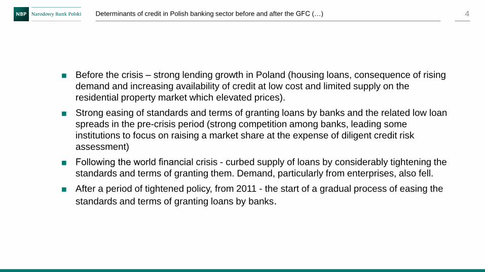
■ Before the crisis – strong lending growth in Poland (housing loans, consequence of rising
demand and increasing availability of credit at low cost and limited supply on the
residential property market which elevated prices).
■ Strong easing of standards and terms of granting loans by banks and the related low loan
spreads in the pre-crisis period (strong competition among banks, leading some
institutions to focus on raising a market share at the expense of diligent credit risk
assessment)
■ Following the world financial crisis - curbed supply of loans by considerably tightening the
standards and terms of granting them. Demand, particularly from enterprises, also fell.
■ After a period of tightened policy, from 2011 - the start of a gradual process of easing the
standards and terms of granting loans by banks.
Determinants of credit in Polish banking sector before and after the GFC (…) 4
This research investigates the problem of most important determinants of bank lending in
Poland before and after the crisis.
The key issue is the role of demand and supply factors in this process:
• Demand or the supply was the main driver of lending growth?
• Or, maybe, both factors influenced the credit in the same way?
Determinants of credit in Polish banking sector before and after the GFC (…)
Aim of the research
5
Disclaimer:
The views expressed herein are those of the author and not necessarily those of the Narodowy Bank Polski
Literature
Determinants of credit in Polish banking sector before and after the GFC (…) 6
2.
data method authors specifics of the analysis country
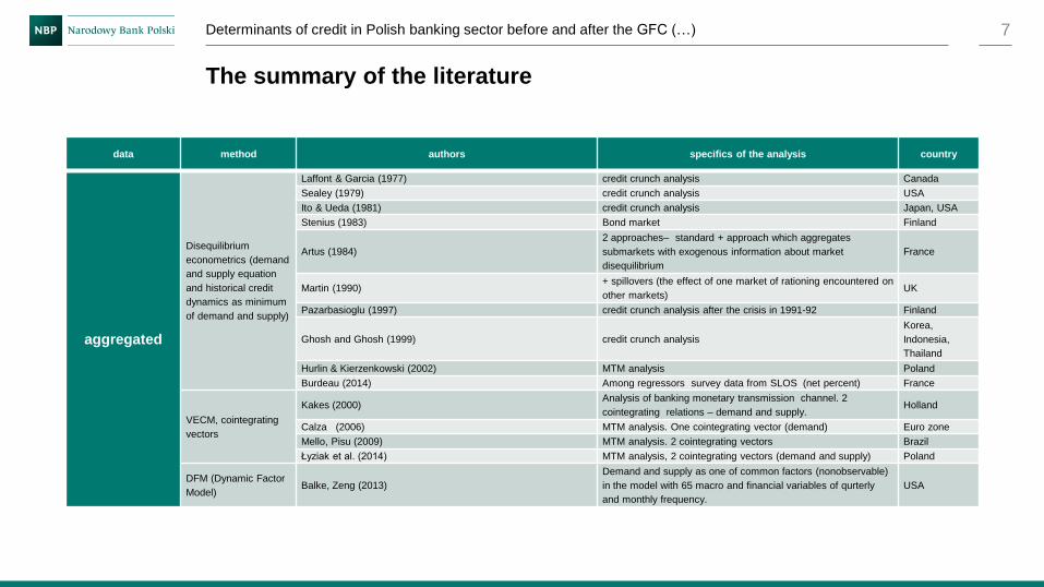
aggregated
Disequilibrium
econometrics (demand
and supply equation
and historical credit
dynamics as minimum
of demand and supply)
Laffont & Garcia (1977) credit crunch analysis Canada
Sealey (1979) credit crunch analysis USA
Ito & Ueda (1981) credit crunch analysis Japan, USA
Stenius (1983) Bond market Finland
Artus (1984)
2 approaches– standard + approach which aggregates
submarkets with exogenous information about market
disequilibrium
France
Martin (1990) + spillovers (the effect of one market of rationing encountered on
other markets) UK
Pazarbasioglu (1997) credit crunch analysis after the crisis in 1991-92 Finland
Ghosh and Ghosh (1999) credit crunch analysis
Korea,
Indonesia,
Thailand
Hurlin & Kierzenkowski (2002) MTM analysis Poland
Burdeau (2014) Among regressors survey data from SLOS (net percent) France
VECM, cointegrating
vectors
Kakes (2000) Analysis of banking monetary transmission channel. 2
cointegrating relations – demand and supply. Holland
Calza (2006) MTM analysis. One cointegrating vector (demand) Euro zone
Mello, Pisu (2009) MTM analysis. 2 cointegrating vectors Brazil
Łyziak et al. (2014) MTM analysis, 2 cointegrating vectors (demand and supply) Poland
DFM (Dynamic Factor
Model) Balke, Zeng (2013)
Demand and supply as one of common factors (nonobservable)
in the model with 65 macro and financial variables of qurterly
and monthly frequency.
USA
Determinants of credit in Polish banking sector before and after the GFC (…) 7
The summary of the literature
data method authors specifics of the analysis country
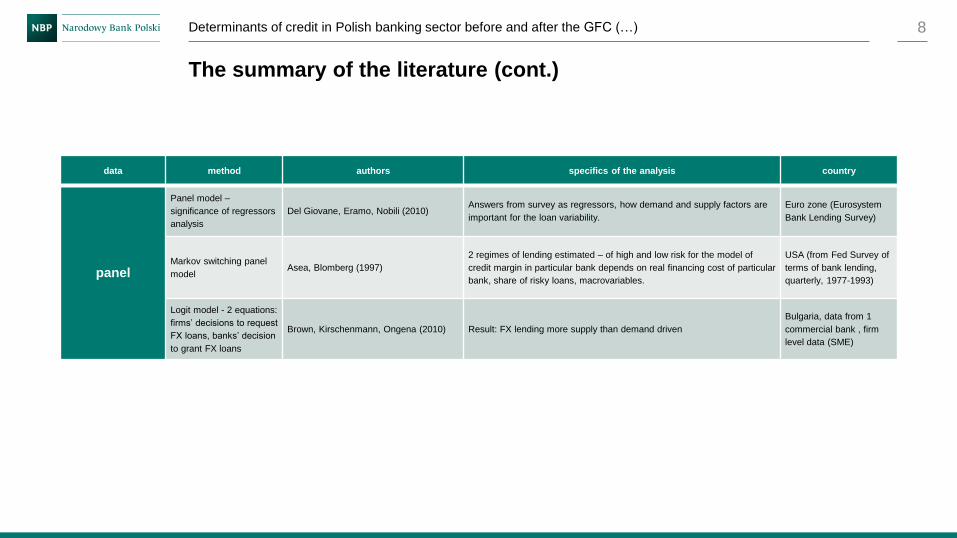
panel
Panel model –
significance of regressors
analysis
Del Giovane, Eramo, Nobili (2010) Answers from survey as regressors, how demand and supply factors are
important for the loan variability.
Euro zone (Eurosystem
Bank Lending Survey)
Markov switching panel
model Asea, Blomberg (1997)
2 regimes of lending estimated – of high and low risk for the model of
credit margin in particular bank depends on real financing cost of particular
bank, share of risky loans, macrovariables.
USA (from Fed Survey of
terms of bank lending,
quarterly, 1977-1993)
Logit model - 2 equations:
firms’ decisions to request
FX loans, banks’ decision
to grant FX loans
Brown, Kirschenmann, Ongena (2010) Result: FX lending more supply than demand driven
Bulgaria, data from 1
commercial bank , firm
level data (SME)
Determinants of credit in Polish banking sector before and after the GFC (…)
8
The summary of the literature (cont.)
Methodology
Determinants of credit in Polish banking sector before and after the GFC (…) 9
3.
2 approaches:
■ time series regression on aggregated data with the use of disequilibrium
econometric approach (regime-switching model)
■ panel regression on disaggregated (bank level) data.
Determinants of credit in Polish banking sector before and after the GFC (…)
Econometric methodology
10

System of separate demand and supply equations together with optimization function (observable volume of credit as minimum of demand and supply):
𝑌𝑡𝑠 = Xt
′α + ξst
𝑌𝑡𝑑 = Zt
′β + ξdt
Qt=Min(𝑌𝑡𝑠, 𝑌𝑡
𝑑)
Q - observable value of loans (dynamics of the stock of loans),
Y - nonobservable values of supply (s) and demand (d),
X - matrix of supply regressors (determinants)
Z - matrix of demand regressors (determinants).
It is also assumed, that vector ξt =(ξst, ξdt)’ is i.i.d. , N 0, Ω where:
Ω = E(ξstξdt′) =𝜎1
2 σ12
σ12 𝜎22
In the process of estimation using Maximum Likelihood method (ML), the vector of structural parameters is estimated: θ = (α β σ1 σ2 σ12)’.
Starting parameters - from one step OLS estimations of separate equations of demand and supply, substituting demand and supply values by historical values of loan dynamics
Disequilibrium econometrics (regime-switching regressions)
11 Determinants of credit in Polish banking sector before and after the GFC (…)
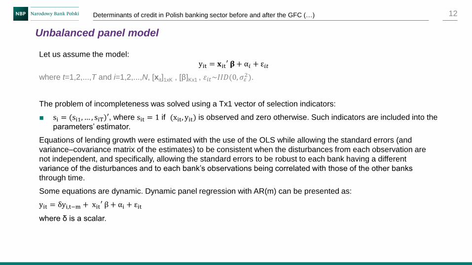
Let us assume the model:
yit = 𝐱it′ 𝛃 + α𝑖 + ε𝑖𝑡
where t=1,2,...,T and i=1,2,...,N, [xit]1xK , [β]Kx1 , 𝜀𝑖𝑡~𝐼𝐼𝐷(0, 𝜎𝜀2).
The problem of incompleteness was solved using a Tx1 vector of selection indicators:
■ si = (si1, … , siT)′, where sit = 1 if (xit, yit) is observed and zero otherwise. Such indicators are included into the
parameters’ estimator.
Equations of lending growth were estimated with the use of the OLS while allowing the standard errors (and
variance–covariance matrix of the estimates) to be consistent when the disturbances from each observation are
not independent, and specifically, allowing the standard errors to be robust to each bank having a different
variance of the disturbances and to each bank’s observations being correlated with those of the other banks
through time.
Some equations are dynamic. Dynamic panel regression with AR(m) can be presented as:
yit = δyi,t−m + xit′ β + αi + εit
where δ is a scalar.
Unbalanced panel model
12 Determinants of credit in Polish banking sector before and after the GFC (…)
Data
Determinants of credit in Polish banking sector before and after the GFC (…) 13
5.

Aggregated:
■ survey (net percent)
■ banking sector data
■ macro data
Disaggregated (bank-level):
■ survey (answers coded from 1 to 5)
■ banking sector data
■ macro data
Determinants of credit in Polish banking sector before and after the GFC (…) 14
Determinants of credit in Polish banking sector before and after the GFC (…)
Aggregated survey data
15
Figure 1
Banks’ lending policy (credit standards) – corporate loans. Aggregated data
from SLOS (net percent).
Figure 2
Banks’ lending policy (credit standards) – loans for households. Aggregated
data from SLOS (net percent).
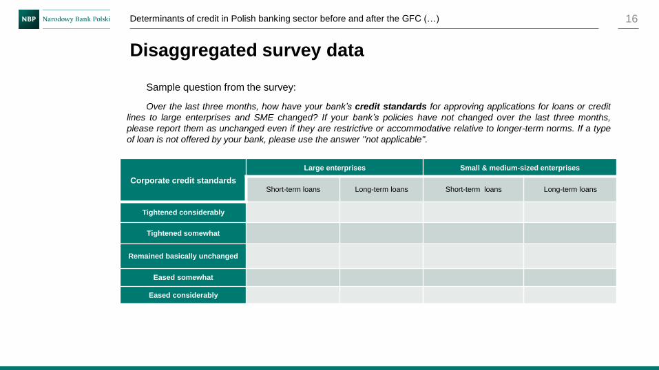
Corporate credit standards
Large enterprises Small & medium-sized enterprises
Short-term loans Long-term loans Short-term loans Long-term loans
Tightened considerably
Tightened somewhat
Remained basically unchanged
Eased somewhat
Eased considerably
Determinants of credit in Polish banking sector before and after the GFC (…)
Disaggregated survey data
16
Sample question from the survey:
Over the last three months, how have your bank’s credit standards for approving applications for loans or credit
lines to large enterprises and SME changed? If your bank’s policies have not changed over the last three months,
please report them as unchanged even if they are restrictive or accommodative relative to longer-term norms. If a type
of loan is not offered by your bank, please use the answer ''not applicable''.

Results
Determinants of credit in Polish banking sector before and after the GFC (…) 17
6.
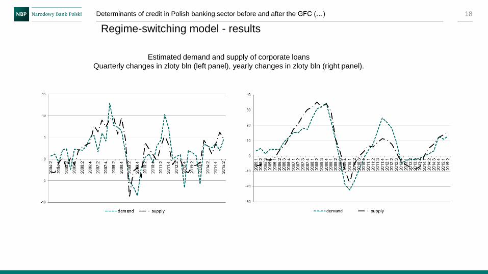
Determinants of credit in Polish banking sector before and after the GFC (…) 18
Estimated demand and supply of corporate loans
Quarterly changes in zloty bln (left panel), yearly changes in zloty bln (right panel).
Regime-switching model - results
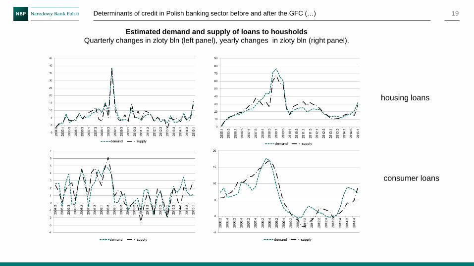
Determinants of credit in Polish banking sector before and after the GFC (…) 19
Estimated demand and supply of loans to housholds
Quarterly changes in zloty bln (left panel), yearly changes in zloty bln (right panel).
housing loans
consumer loans
Determinants of credit in Polish banking sector before and after the GFC (…) 20
Regime-switching model - results
Estimated probability of demand and supply regimes – corporate loans.
Estimated probability of demand and supply regimes – housing loans.
Estimated probability of demand and supply regimes – consumer loans.
Before the Crisis After the Crisis
Coef. Std. z P>z [95% Conf.
Interval] Coef. Std. z P>z [95% Conf. Interval]
STANDARDS_LCSHORT 1.238 1.914 0.650 0.518 -2.512 4.989 14.825 5.701 2.600 0.009 3.651 25.998
STANDARDS_LCLONG -0.298 1.756 -0.170 0.865 -3.739 3.143 7.489 4.743 1.580 0.114 -1.806 16.784
STANDARDS_SMESHORT 1.270 1.170 1.090 0.278 -1.023 3.563 -14.643 4.070 -3.600 0.000 -22.620 -6.665
STANDARDS_SMELONG -0.723 0.975 -0.740 0.459 -2.634 1.189 -13.754 4.391 -3.130 0.002 -22.360 -5.148
DEMAND_LCSHORT -1.165 1.330 -0.880 0.381 -3.772 1.442 -0.018 3.913 0.000 0.996 -7.688 7.652
DEMAND_LCLONG 2.011 1.402 1.430 0.151 -0.736 4.758 5.968 5.244 1.140 0.255 -4.309 16.246
DEMAND_SMESHORT 0.328 1.362 0.240 0.809 -2.342 2.998 -4.675 3.326 -1.410 0.160 -11.194 1.843
DEMAND_SMELONG -1.639 1.553 -1.060 0.291 -4.684 1.406 -8.569 3.941 -2.170 0.030 -16.293 -0.844
SUPPLYF_LCSHORT(-1) -1.422 2.158 -0.660 0.510 -5.651 2.807 -5.987 6.578 -0.910 0.363 -18.879 6.905
SUPPLYF_LCLONG(-1) -1.276 1.738 -0.730 0.463 -4.682 2.130 -1.459 4.950 -0.290 0.768 -11.161 8.244
SUPPLYF_SMELONG(-1) 0.459 1.861 0.250 0.805 -3.189 4.107 3.723 5.274 0.710 0.480 -6.613 14.060
SUPPLYF_SMESHORT(-1) 1.659 1.732 0.960 0.338 -1.736 5.055 8.075 5.281 1.530 0.126 -2.275 18.426
DEMANDF_LCSHORT 1.490 1.469 1.010 0.310 -1.389 4.370 -4.172 7.159 -0.580 0.560 -18.203 9.860
DEMANDF_LCLONG -1.325 1.609 -0.820 0.410 -4.479 1.829 -5.066 6.343 -0.800 0.424 -17.498 7.365
DEMANDF_SMESHORT -1.479 1.470 -1.010 0.314 -4.361 1.403 4.188 6.261 0.670 0.504 -8.083 16.459
DEMANDF_SMELONG -0.792 1.257 -0.630 0.529 -3.256 1.672 6.171 7.337 0.840 0.400 -8.209 20.550
dummies
cons 10.825 6.655 1.630 0.104 -2.218 23.868 22.392 9.864 2.270 0.023 3.059 41.726
Determinants of credit in Polish banking sector before and after the GFC (…) 21
Only survey data as regressors
Panel regressions - results
Results of estimation of the equation of corporate loans growth
Before the Crisis After the Crisis
Coef. Std.
Err. z P>z [95% Conf. Interval] Coef. Std. Err. z P>z
[95% Conf.
Interval]
GLOANSCR(-4) 0.082 0.072 1.140 0.254 -0.059 0.223 0.041 0.216 0.190 0.848 -0.381 0.464
SUPPLYF_
SMESHORT(-1) 1.482 1.102 1.340 0.179 -0.679 3.642 5.330 2.634 2.020 0.043 0.167 10.494
SUPPLYF_
SMESHORT(-3) -0.190 1.073 -0.180 0.860 -2.293 1.913 3.611 1.454 2.480 0.013 0.760 6.461
GRGDP(-2) 1.047 0.718 1.460 0.145 -0.359 2.454 -2.760 1.615 -1.710 0.088 -5.926 0.406
minimis (omitted) 2.234 4.657 0.480 0.631 -6.893 11.361
dummies
(mergers)
_cons -4.849 7.351 -0.660 0.509 -19.256 9.559 -13.169 8.325 -1.580 0.114 -29.486 3.148
Selected equation from equations with survey, banking and macro data as regressors
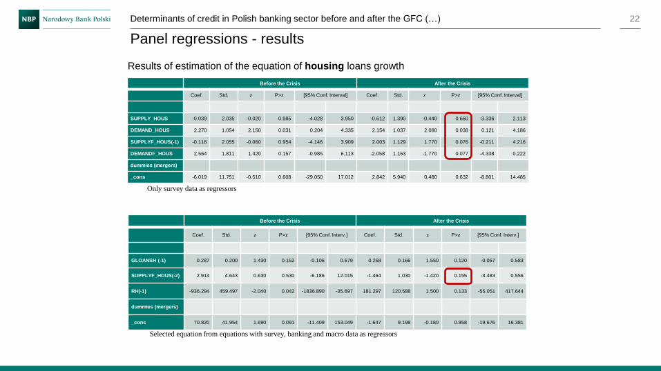
Determinants of credit in Polish banking sector before and after the GFC (…) 22
Only survey data as regressors
Panel regressions - results
Results of estimation of the equation of housing loans growth
Selected equation from equations with survey, banking and macro data as regressors
Before the Crisis After the Crisis
Coef. Std. z P>z [95% Conf. Interv.] Coef. Std. z P>z [95% Conf. Interv.]
GLOANSH (-1) 0.287 0.200 1.430 0.152 -0.106 0.679 0.258 0.166 1.550 0.120 -0.067 0.583
SUPPLYF_HOUS(-2) 2.914 4.643 0.630 0.530 -6.186 12.015 -1.464 1.030 -1.420 0.155 -3.483 0.556
RH(-1) -936.294 459.497 -2.040 0.042 -1836.890 -35.697 181.297 120.588 1.500 0.133 -55.051 417.644
dummies (mergers)
_cons 70.820 41.954 1.690 0.091 -11.409 153.049 -1.647 9.198 -0.180 0.858 -19.676 16.381
Before the Crisis After the Crisis
Coef. Std. z P>z [95% Conf. Interval] Coef. Std. z P>z [95% Conf. Interval]
SUPPLY_HOUS -0.039 2.035 -0.020 0.985 -4.028 3.950 -0.612 1.390 -0.440 0.660 -3.336 2.113
DEMAND_HOUS 2.270 1.054 2.150 0.031 0.204 4.335 2.154 1.037 2.080 0.038 0.121 4.186
SUPPLYF_HOUS(-1) -0.118 2.055 -0.060 0.954 -4.146 3.909 2.003 1.129 1.770 0.076 -0.211 4.216
DEMANDF_HOUS 2.564 1.811 1.420 0.157 -0.985 6.113 -2.058 1.163 -1.770 0.077 -4.338 0.222
dummies (mergers)
_cons -6.019 11.751 -0.510 0.608 -29.050 17.012 2.842 5.940 0.480 0.632 -8.801 14.485
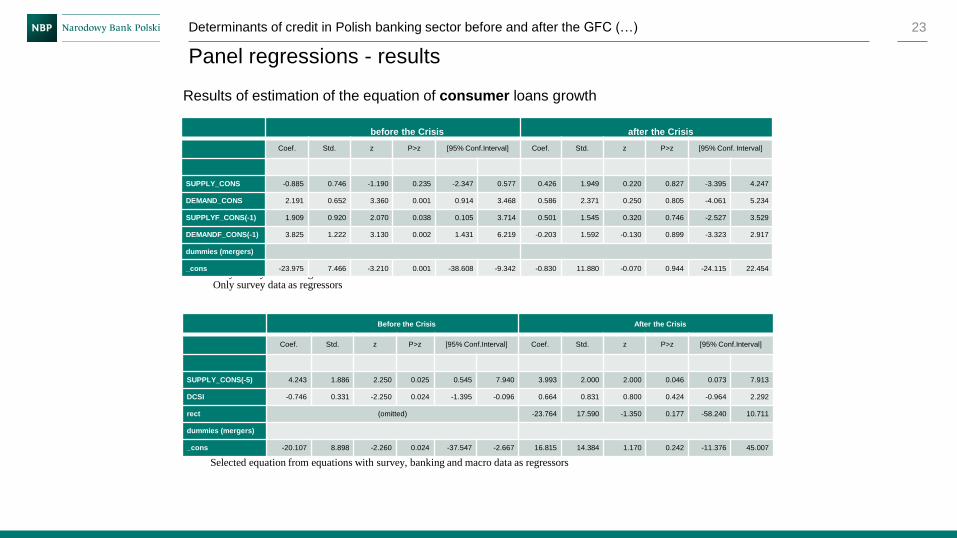
Determinants of credit in Polish banking sector before and after the GFC (…) 23
Only survey data as regressors
Panel regressions - results
Results of estimation of the equation of consumer loans growth
Selected equation from equations with survey, banking and macro data as regressors
Before the Crisis After the Crisis
Coef. Std. z P>z [95% Conf.Interval] Coef. Std. z P>z [95% Conf.Interval]
SUPPLY_CONS(-5) 4.243 1.886 2.250 0.025 0.545 7.940 3.993 2.000 2.000 0.046 0.073 7.913
DCSI -0.746 0.331 -2.250 0.024 -1.395 -0.096 0.664 0.831 0.800 0.424 -0.964 2.292
rect (omitted) -23.764 17.590 -1.350 0.177 -58.240 10.711
dummies (mergers)
_cons -20.107 8.898 -2.260 0.024 -37.547 -2.667 16.815 14.384 1.170 0.242 -11.376 45.007
before the Crisis after the Crisis
Coef. Std. z P>z [95% Conf.Interval] Coef. Std. z P>z [95% Conf. Interval]
SUPPLY_CONS -0.885 0.746 -1.190 0.235 -2.347 0.577 0.426 1.949 0.220 0.827 -3.395 4.247
DEMAND_CONS 2.191 0.652 3.360 0.001 0.914 3.468 0.586 2.371 0.250 0.805 -4.061 5.234
SUPPLYF_CONS(-1) 1.909 0.920 2.070 0.038 0.105 3.714 0.501 1.545 0.320 0.746 -2.527 3.529
DEMANDF_CONS(-1) 3.825 1.222 3.130 0.002 1.431 6.219 -0.203 1.592 -0.130 0.899 -3.323 2.917
dummies (mergers)
_cons -23.975 7.466 -3.210 0.001 -38.608 -9.342 -0.830 11.880 -0.070 0.944 -24.115 22.454
Only survey data as regressors
Determinants of credit in Polish banking sector before and after the GFC (…) 24
Panel regressions - results
consumer loans
Estimation of growth of consumer loans in two subsamples of both equations has shown decrease
of information value of both demand and supply factors in the second subsample (significance of
demand and supply factors decreased after the Crisis).
Estimations of both specifications in two subsamples suggest the strong rise of significance of
supply factors of credit in the period after the Crisis.
corporate loans
housing loans
In case of segment of housing loans, the conclusions are quite similar to corporate, however the
rise in significance of supply factors is smaller. But in fact, in the period after the Crisis, answers
on the questions concerning supply had higher values of the test of significance
Conclusions
Determinants of credit in Polish banking sector before and after the GFC(…) 25
7.
The results received on the bank-level data:
■ increasing significance of supply factors after the Crisis in case of corporate and
housing loans.
Results on aggregated data with the use of regime-switching model
■ higher importance of supply side in determining the credit growth in case of
corporate loans and consumer loan segment after the Crisis.
Determinants of credit in Polish banking sector before and after the GFC (…) 26