Embed Size (px)
Citation preview

Prof. Dr. Barbara Wohlmuth
Lehrstuhl fur Numerische Mathematik
Die Interpolationsformel von Lagrange
Zentrale Aussage: Zu beliebigen n + 1 Stutzpunkten (xi, fi), i = 0, . . . , n mitpaarweise verschiedenen Stutzstellen xi 6= xj, fur i 6= j, gibt es genau ein Polynomπn ∈ Pn mit
πn(xi) = fi, i = 0, . . . , n.
Es gilt
πn(x) =n∑
i=0
fiLi(x)
mit den Interpolationspolynomen
Li(x) :=∏
k 6=i
x− xk
xi − xk, i = 0, . . . , n.
Polynominterpolation (interpol02) 1

Prof. Dr. Barbara Wohlmuth
Lehrstuhl fur Numerische Mathematik
Die Interpolationsformel von Lagrange, Beispiel
Gegeben seien fur n = 2 :
i 0 1 2xi 0 1 3fi 1 3 2
Als Interpolationspolynome ergeben sich
L0(x) =(x− 1)(x− 3)
(0− 1)(0− 3), L1(x) =
(x− 0)(x− 3)
(1− 0)(1− 3), L2(x) =
(x− 0)(x− 1)
(3− 0)(3− 1),
und damit
π2(x) = 1 · L0(x) + 3 · L1(x) + 2 · L2(x)
=1
6(−5x2 + 17x+ 6)
-6
-5
-4
-3
-2
-1
0
1
2
3
4
-1 0 1 2 3 4
P(x)1L0(x)3L1(x)2L2(x)
Stuetzstellen
Polynominterpolation (interpol03) 2

Prof. Dr. Barbara Wohlmuth
Lehrstuhl fur Numerische Mathematik
Die Interpolationsformel von Lagrange
Beispiel: Exponentialfunktion
Gegeben seien fur n = 2 :
i 0 1 2xi −1 0 1fi e−1 e0 e1
Als Interpolationspolynome ergeben sich
L0(x) =(x − 0)(x − 1)
(−1 − 1)(−1 − 0), L1(x) =
(x + 1)(x − 1)
(0 + 1)(0 − 1), L2(x) =
(x + 1)(x − 0)
(1 + 1)(1 − 0),
und damit
π2(x) = e−1 · L0(x) + e0 · L1(x) + e1 · L2(x)
= e−1 ·1
2(x2 − x)− 1 · (x2 − 1) + e ·
1
2(x2 + x)
=
(
1
2e− 1 +
e
2
)
x2 +
(
e
2−
1
2e
)
x+ 1
= (cosh(1)− 1)x2 + sinh(1)x+ 1
Polynominterpolation (interpol03a) 3

Prof. Dr. Barbara Wohlmuth
Lehrstuhl fur Numerische Mathematik
Die Interpolationsformel von Lagrange
Beispiel: Exponentialfunktion
−2 −1 0 1 2−2
−1
0
1
2
3
4 L0(x)
L1(x)
L2(x)
Stützpunkte
−2 −1 0 1 2
0
2
4
6
8 Π2(x)
ex
e−1*L0(x)
e0*L1(x)
e1*L2(x)
Stützstellen
Polynominterpolation (interpol04a) 4

Prof. Dr. Barbara Wohlmuth
Lehrstuhl fur Numerische Mathematik
Interpolationsfehler
Die Stutzwerte fi stammen oft von einer stetigen Funktion f , d.h.
fi = f(xi), i = 0, . . . , n.
Gilt {xi : i = 0, . . . , n} ⊂ [a, b], so lasst sich der Fehler f − πn in derMaximumsnorm
‖f‖[a,b] := ‖f‖L∞([a,b]) := maxx∈[a,b]
|f(x)|
abschatzen als
‖f − πn‖[a,b] ≤‖ωn+1‖[a,b](n+ 1)!
‖f (n+1)‖[a,b].
Hierbei ist
ωn+1(x) :=
n∏
i=0
(x− xi).
Der Ausdruck ‖ωn+1‖[a,b] hangt alleine von der Wahl der Stutzstellen ab.
Polynominterpolation (interpol11) 5

Prof. Dr. Barbara Wohlmuth
Lehrstuhl fur Numerische Mathematik
Das Polynom ωn+1
Aquidistante Stutzstellen, n = 21
−1 −0.5 0 0.5 1−20
−15
−10
−5
0
5x 10⁻⁵
Frage: Gibt es eine Knotenverteilung, so dass ‖ωn+1‖[a,b] minimal wird?
Polynominterpolation (interpol12) 6
Prof. Dr. Barbara Wohlmuth
Lehrstuhl fur Numerische Mathematik
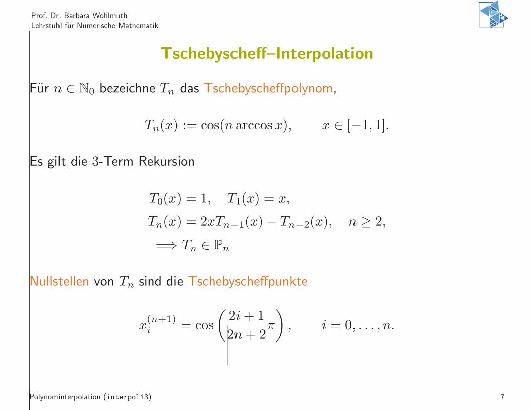
Tschebyscheff–Interpolation
Fur n ∈ N0 bezeichne Tn das Tschebyscheffpolynom,
Tn(x) := cos(n arccosx), x ∈ [−1, 1].
Es gilt die 3-Term Rekursion
T0(x) = 1, T1(x) = x,
Tn(x) = 2xTn−1(x)− Tn−2(x), n ≥ 2,
=⇒ Tn ∈ Pn
Nullstellen von Tn sind die Tschebyscheffpunkte
x(n+1)i = cos
(
2i+ 1
2n+ 2π
)
, i = 0, . . . , n.
Polynominterpolation (interpol13) 7

Prof. Dr. Barbara Wohlmuth
Lehrstuhl fur Numerische Mathematik
Tschebyscheffpunkte
n = 3
45
n = 5
30
20
n = 8 n=17
10
Polynominterpolation (interpol14) 8

Prof. Dr. Barbara Wohlmuth
Lehrstuhl fur Numerische Mathematik
Das Polynom ωn+1
Tschebyscheffknoten, n = 21
−1 −0.5 0 0.5 1−5
0
5x 10⁻⁷
‖ω22,aqui‖[−1,1]
‖ω22,cheb‖[−1,1]≈ 3.5 · 102
z.B. n = 40
‖ω41,aqui‖[−1,1]
‖ω41,cheb‖[−1,1]≈ 3.3 · 105
allgemein
‖ωn+1,cheb‖[−1,1] = 2−n
Polynominterpolation (interpol15) 9

Prof. Dr. Barbara Wohlmuth
Lehrstuhl fur Numerische Mathematik
Das Polynom ωn+1
‖ωn+1‖∞;[−1,1] fur verschiedene Stutzstellen
0 200 400 60010
−200
10−100
100
10100
10200
||ω||∞;[−1,1]
Anzahl Stützstellen
äquidistant
nur in [0,1]
nur in [−1,−0.5]∪ [0.5,1]
...+ einige in [−0,5,0.5]
Tschebyscheff
Polynominterpolation (interpol15a) 10

Prof. Dr. Barbara Wohlmuth
Lehrstuhl fur Numerische Mathematik
Aquidistante Punkte vs. Tschebyscheffpunkte
−1 −0.5 0 0.5 1−0.5
0
0.5
1
1.5
2
2.5
3n = 19, Lagrange Polynom L
9(x)
‖L9,aquidistant‖[−1,1] = 1.0 · 103, ‖L9,Tschebyscheff‖[−1,1] = 1.0
Polynominterpolation (interpol17) 11
Prof. Dr. Barbara Wohlmuth
Lehrstuhl fur Numerische Mathematik
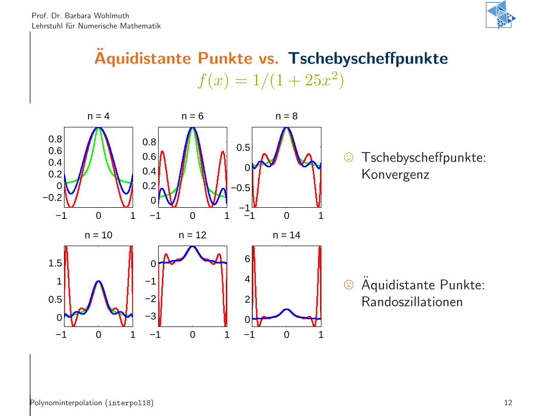
Aquidistante Punkte vs. Tschebyscheffpunkte
f(x) = 1/(1 + 25x2)
−1 0 1
−0.20
0.20.40.60.8
n = 4
−1 0 1
0
0.2
0.4
0.6
0.8
n = 6
−1 0 1−1
−0.5
0
0.5
n = 8
−1 0 1
0
0.5
1
1.5
n = 10
−1 0 1
−3
−2
−1
0
n = 12
−1 0 1
0
2
4
6
n = 14
, Tschebyscheffpunkte:Konvergenz
/ Aquidistante Punkte:Randoszillationen
Polynominterpolation (interpol18) 12
Prof. Dr. Barbara Wohlmuth
Lehrstuhl fur Numerische Mathematik
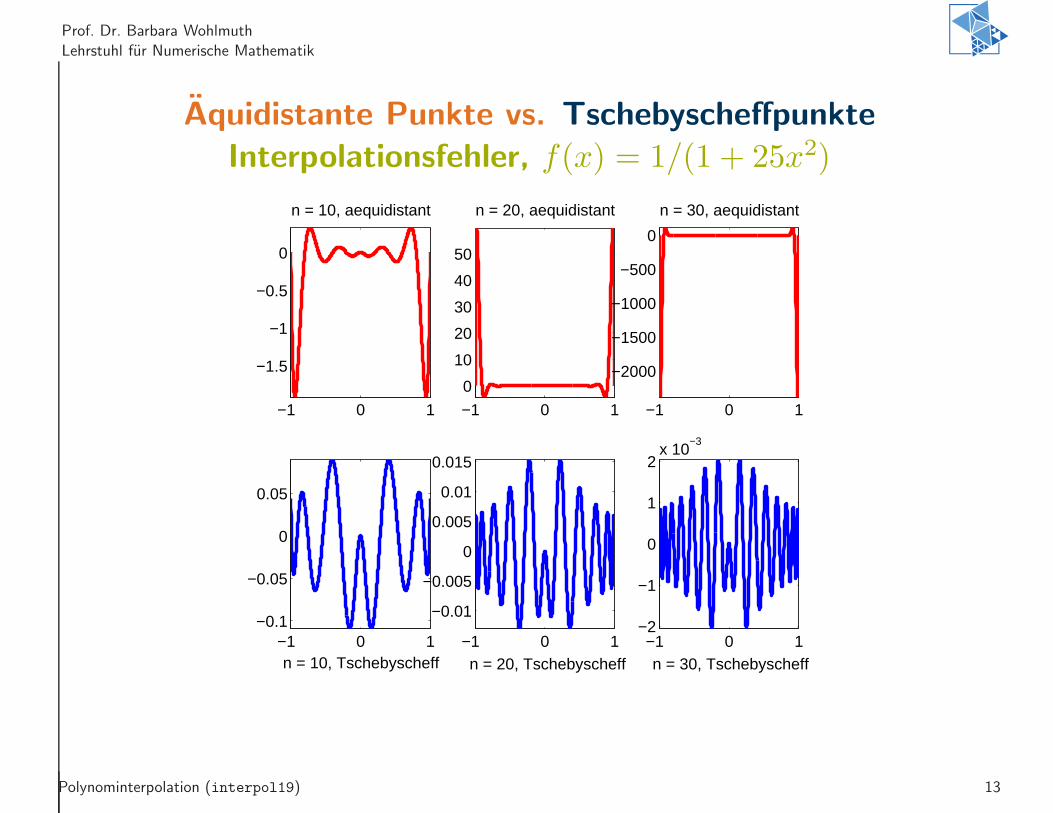
Aquidistante Punkte vs. Tschebyscheffpunkte
Interpolationsfehler, f(x) = 1/(1 + 25x2)
−1 0 1
−1.5
−1
−0.5
0
n = 10, aequidistant
−1 0 1−0.1
−0.05
0
0.05
n = 10, Tschebyscheff
−1 0 1
0
10
20
30
40
50
n = 20, aequidistant
−1 0 1
−0.01
−0.005
0
0.005
0.01
0.015
n = 20, Tschebyscheff
−1 0 1
−2000
−1500
−1000
−500
0
n = 30, aequidistant
−1 0 1−2
−1
0
1
2x 10
−3
n = 30, Tschebyscheff
Polynominterpolation (interpol19) 13

Prof. Dr. Barbara Wohlmuth
Lehrstuhl fur Numerische Mathematik
Aquidistante Punkte vs. Tschebyscheffpunkte f(x) = |x|3/2
−1 0 1
0.2
0.4
0.6
0.8
1n = 4
−1 0 1
0.2
0.4
0.6
0.8
1n = 6
−1 0 1
0.2
0.4
0.6
0.8
1n = 8
−1 0 1
0.2
0.4
0.6
0.8
1n = 10
−1 0 1
0.2
0.4
0.6
0.8
1
1.2
n = 12
−1 0 1
0.2
0.4
0.6
0.8
1n = 14
Polynominterpolation (interpol20) 14

Prof. Dr. Barbara Wohlmuth
Lehrstuhl fur Numerische Mathematik
Aquidistante Punkte vs. Tschebyscheffpunkte f(x) =√
|x|
−1 0 1
0.20.40.60.8
11.2
n = 4
−1 0 1
0.2
0.4
0.6
0.8
1
n = 6
−1 0 1
0.5
1
1.5
n = 8
−1 0 1−1
0
1
n = 10
−1 0 1
2
4
6
n = 12
−1 0 1
−10
−5
0
n = 14
Polynominterpolation (interpol20a) 15
Prof. Dr. Barbara Wohlmuth
Lehrstuhl fur Numerische Mathematik
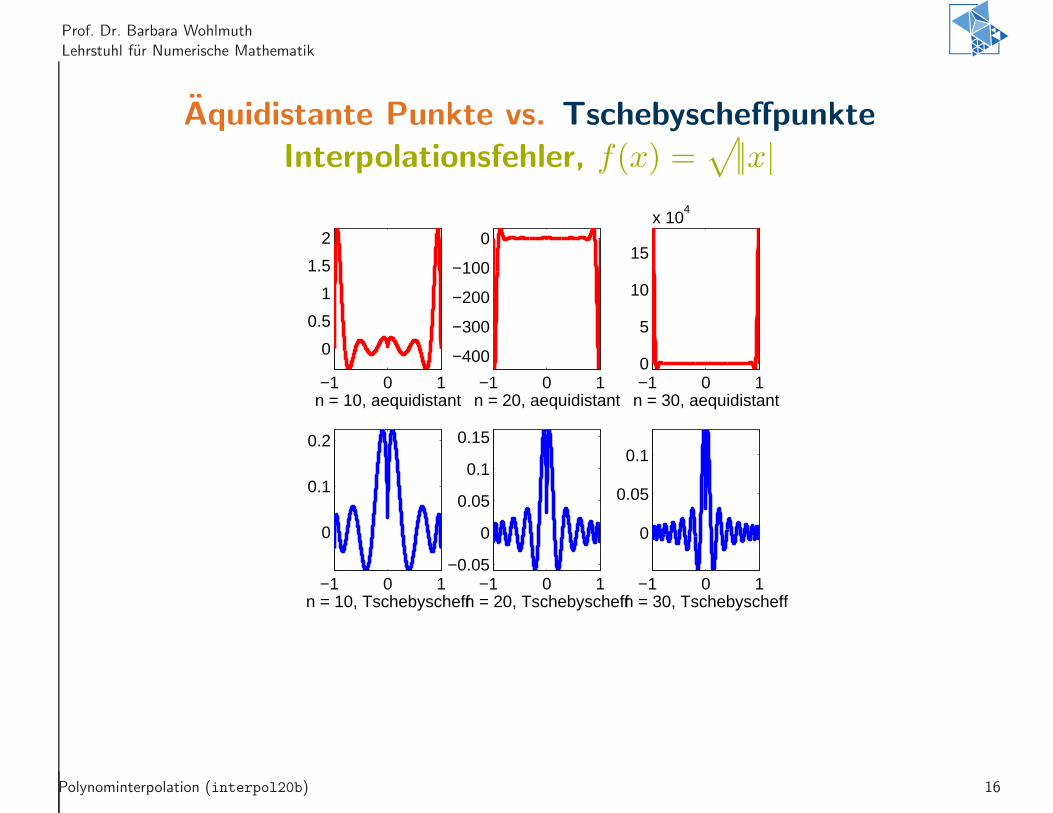
Aquidistante Punkte vs. Tschebyscheffpunkte
Interpolationsfehler, f(x) =√
|x|
−1 0 1
0
0.5
1
1.5
2
n = 10, aequidistant
−1 0 1
0
0.1
0.2
n = 10, Tschebyscheff
−1 0 1
−400
−300
−200
−100
0
n = 20, aequidistant
−1 0 1−0.05
0
0.05
0.1
0.15
n = 20, Tschebyscheff
−1 0 10
5
10
15
x 104
n = 30, aequidistant
−1 0 1
0
0.05
0.1
n = 30, Tschebyscheff
Polynominterpolation (interpol20b) 16

Prof. Dr. Barbara Wohlmuth
Lehrstuhl fur Numerische Mathematik
Interpolationsfehler und Lebesgue Konstanten Λn
Definiton Lebesgue Konstante Λn:
Λn := maxx∈[−1,1]
n∑
i=0
|Li(x)|
Interpolationsfehler:
‖f −Πnf‖[−1,1] ≤ CΛnω(f,1
n)
Hierbei bezeichnen Li die Lagrange-Interpolationspolynome, und ω(f, 1n) denStetigkeitsmodul von f . Dieser ist definiert als
ω(f, δ) := sup|x−y|<δ
|f(x)− f(y)|
mit ω(f, 1n) ≤Ln falls f Lipschitz-stetig hinsichtlich der Konstanten L ist.
Polynominterpolation (interpol20c) 17

Prof. Dr. Barbara Wohlmuth
Lehrstuhl fur Numerische Mathematik
Verhalten der Lebesgue-Konstanten fur steigende
Polynomordnung
Aquidistant vs. Tschebyscheff
0 10 20 3010
0
105
1010
Lebesgue−Konstante
Anzahl Stützstellen
äquidistantTschebyscheff
0 10 20 30
100.3
100.4
100.5
Lebesgue−Konstante
Anzahl Stützstellen
Tschebyscheff(2/π)*log(n+1)+1
, Λn wachst logarithmisch fur Tschebyscheffpunkte: Λn ≤ 2π ln(n+ 1) + 1,
/ Λn wachst exponentiell fur aquidistante Punkte: Λn ≥ Cen/2.
Polynominterpolation (interpol15b) 18

Prof. Dr. Barbara Wohlmuth
Lehrstuhl fur Numerische Mathematik
Konvergenzverhalten fur Tschebyscheffpunkte
Interpolationsfehler ‖f(x)−Πn(x)‖[−1,1]
0 500 100010
−15
10−10
10−5
100
Fehler (logarithmisch)
Anzahl Stützstellen
1/(1+25x2)
|x|3/2
|x|1/2
Interpolationsfehler hangt vom Stetigkeitsmodul ω(f, 1n) des Interpolanden ab.
Polynominterpolation (interpol20d) 19

Prof. Dr. Barbara Wohlmuth
Lehrstuhl fur Numerische Mathematik
Konvergenzverhalten fur Tschebyscheffpunkte
Interpolationspolynom fur f(x) = 1/| ln |x/2||
Gerade Anzahl Stutzstellen Ungerade Anzahl Stutzstellen
−1 −0.5 0 0.5 10
0.5
1
1.5|ln|x/2||−1
Π5(x)
−1 −0.5 0 0.5 10
0.5
1
1.5|ln|x/2||−1
Π6(x)
Polynominterpolation (interpol20g) 20

Prof. Dr. Barbara Wohlmuth
Lehrstuhl fur Numerische Mathematik
Aquidistante Punkte vs. Tschebyscheffpunkte
Interpolationsfehler, f(x) = |x|3/2
−1 0 1
0
0.05
0.1
n = 10, aequidistant
−1 0 1
−5
0
5
10x 10
−3
n = 10, Tschebyscheff
−1 0 1
−10
−5
0
n = 20, aequidistant
−1 0 1−2
−1
0
1
2
3
x 10−3
n = 20, Tschebyscheff
−1 0 10
1000
2000
3000
n = 30, aequidistant
−1 0 1
−1
0
1
2x 10
−3
n = 30, Tschebyscheff
Polynominterpolation (interpol21) 21

Prof. Dr. Barbara Wohlmuth
Lehrstuhl fur Numerische Mathematik
Weierstrassfunktion fur Tschebyscheffpunkte
w(x) =∑∞
k=0 ak cos(2πbkx) mit a = 1/2 und b = 3
−1 −0.5 0 0.5 1−2
−1
0
1
2Weierstrassfunktion
w(x)π
40(x)
0 500 100010
−2
10−1
100
101
Fehler (logarithmisch)
Anzahl Stützstellen
/ Weierstrassfunktion nirgends differenzierbar.
/ Interpolation fur pathologische Funktionen nicht konvergent.
Polynominterpolation (interpol20e) 22

Prof. Dr. Barbara Wohlmuth
Lehrstuhl fur Numerische Mathematik
Baryzentrische Lagrange Interpolation
Ziel: Weitere Methode vom Aufwand relativ gering, aber numerisch stabil.Berechne das Lagrangesche Interpolationspolynom πn(x) zu der Funktion f :[a, b] → R zu den Stutzstellen xj, j = 0, 1, ..., n.Definiere die baryzentrischen Gewichte durch
ωj :=1
∏nk=0;k 6=j(xj − xk)
, j = 0, 1, ..., n.
Dann kann das Lagrangesche Interpolationspolynom durch
πn(x) :=
∑nj=0
ωj
x−xjf(xj)
∑nj=0
ωj
x−xj
dargestellt werden.
Polynominterpolation (interpol83) 23
Prof. Dr. Barbara Wohlmuth
Lehrstuhl fur Numerische Mathematik
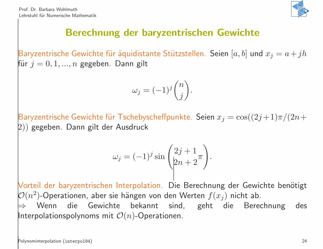
Berechnung der baryzentrischen Gewichte
Baryzentrische Gewichte fur aquidistante Stutzstellen. Seien [a, b] und xj = a+ jhfur j = 0, 1, ..., n gegeben. Dann gilt
ωj = (−1)j(
n
j
)
.
Baryzentrische Gewichte fur Tschebyscheffpunkte. Seien xj = cos((2j+1)π/(2n+2)) gegeben. Dann gilt der Ausdruck
ωj = (−1)j sin
(
2j + 1
2n+ 2π
)
.
Vorteil der baryzentrischen Interpolation. Die Berechnung der Gewichte benotigtO(n2)-Operationen, aber sie hangen von den Werten f(xj) nicht ab.⇒ Wenn die Gewichte bekannt sind, geht die Berechnung desInterpolationspolynoms mit O(n)-Operationen.
Polynominterpolation (interpol84) 24

Prof. Dr. Barbara Wohlmuth
Lehrstuhl fur Numerische Mathematik
Das Schema von Aitken und Neville
Das gesuchte Polynom πn soll an einem Punkt x ausgewertet werden. Fur k + 1paarweise verschiedene Indizes {i0, . . . , ik} ⊂ {0, . . . , n} bezeichne Pi0...ik ∈ Pk
das Interpolationspolynom durch (xi0, fi0), . . . , (xik, fik). Es gilt:
Pi(x) = fi, i = 0, . . . , n,
Pi0...ik(x) =(x− xi0)Pi1...ik(x)− (x− xik)Pi0...ik−1
(x)
xik − xi0
.
Neville–Schema fur n = 2:
k = 0 1 2
x0 f0 = P0(x)
P01(x)
x1 f1 = P1(x) P012(x)
P12(x)
x2 f2 = P2(x)
Polynominterpolation (interpol05) 25

Prof. Dr. Barbara Wohlmuth
Lehrstuhl fur Numerische Mathematik
Das Schema von Aitken und Neville, Beispiel
Gegeben seien fur n = 2 :
i 0 1 2xi 0 1 3fi 1 3 2
Neville–Schema fur die Berechnung von π2(2) = P012(2):
k = 0 1 2
x0 = 0 P0(2) = 1
P01(2) = (2−0)·3−(2−1)·11−0 = 5
x1 = 1 P1(2) = 3 P012(2) = (2−0)·5/2−(2−3)·53−0 = 10/3
P12(2) = (2−1)·2−(2−3)·33−1 = 5/2
x2 = 3 P2(2) = 2
Polynominterpolation (interpol06) 26

Prof. Dr. Barbara Wohlmuth
Lehrstuhl fur Numerische Mathematik
Das Schema von Aitken und Neville
Einfache Erweiterung um zusatzliche Punkte
zusatzliches Wertepaar (x3, f3) := (4, 3), berechne π3(2) = P0123(2):
k = 0 1 2 3
x0 = 0 P0(2) = 1
P01(2) = 5
x1 = 1 P1(2) = 3 P012(2) = 10/3
P12(2) = 5/2 P0123(2) = 8/3
x2 = 3 P2(2) = 2 P123(2) = 2
P23(2) = 1
x3 = 4 P3(2) = 3
Polynominterpolation (interpol07) 27

Prof. Dr. Barbara Wohlmuth
Lehrstuhl fur Numerische Mathematik
Die Newtonsche Interpolationsformel
Idee: Darstellung des gesuchten Polynoms πn als
πn(x) = c0 + c1(x− x0) + c2(x− x0)(x− x1) + . . .+ cn(x− x0) · · · (x− xn−1)
=
n∑
i=0
ci
i−1∏
k=0
(x− xk).
Bestimmung der Koeffizienten ci, i = 0, . . . , n durch
f0 = πn(x0) = c0
f1 = πn(x1) = c0 + c1(x1 − x0)
...
fn = πn(xn) = c0 + c1(xn − x0) + . . .+ cn
n−1∏
k=0
(xn − xk)
Polynominterpolation (interpol08) 28
Prof. Dr. Barbara Wohlmuth
Lehrstuhl fur Numerische Mathematik
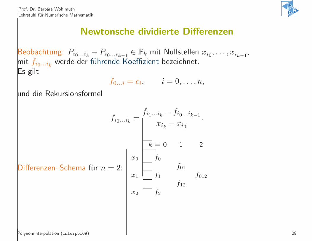
Newtonsche dividierte Differenzen
Beobachtung: Pi0...ik − Pi0...ik−1∈ Pk mit Nullstellen xi0, . . . , xik−1
,mit fi0...ik werde der fuhrende Koeffizient bezeichnet.Es gilt
f0...i = ci, i = 0, . . . , n,
und die Rekursionsformel
fi0...ik =fi1...ik − fi0...ik−1
xik − xi0
.
Differenzen–Schema fur n = 2:
k = 0 1 2
x0 f0f01
x1 f1 f012f12
x2 f2
Polynominterpolation (interpol09) 29
Prof. Dr. Barbara Wohlmuth
Lehrstuhl fur Numerische Mathematik
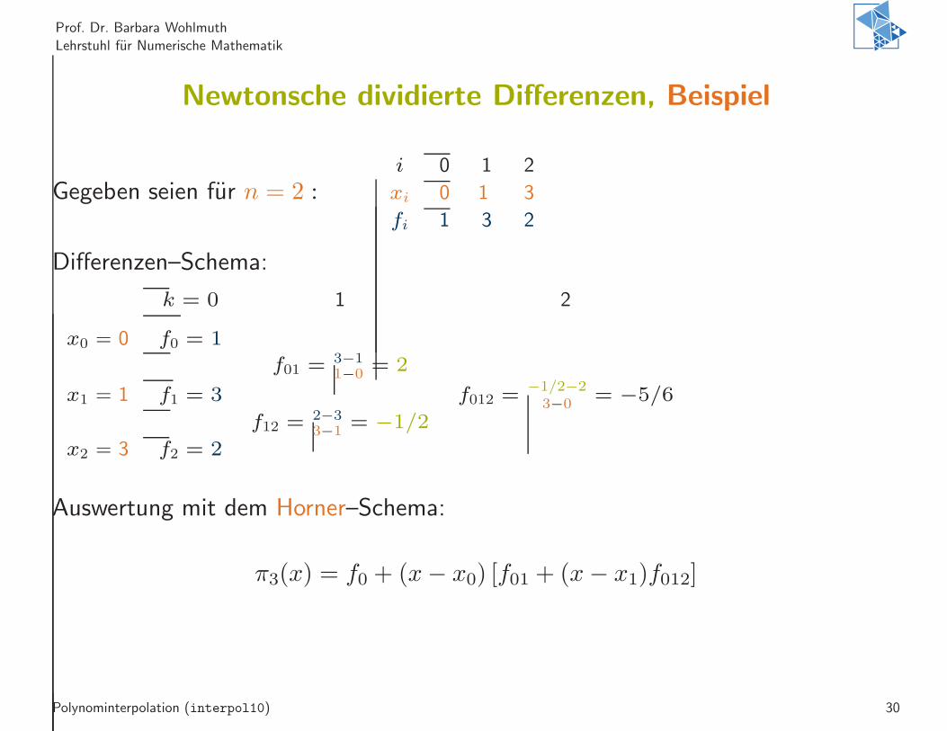
Newtonsche dividierte Differenzen, Beispiel
Gegeben seien fur n = 2 :i 0 1 2
xi 0 1 3
fi 1 3 2
Differenzen–Schema:
k = 0 1 2
x0 = 0 f0 = 1
f01 = 3−11−0 = 2
x1 = 1 f1 = 3 f012 = −1/2−23−0 = −5/6
f12 = 2−33−1 = −1/2
x2 = 3 f2 = 2
Auswertung mit dem Horner–Schema:
π3(x) = f0 + (x− x0) [f01 + (x− x1)f012]
Polynominterpolation (interpol10) 30

Prof. Dr. Barbara Wohlmuth
Lehrstuhl fur Numerische Mathematik
Vergleich Interpolationsfehler, f(x) = 1/(1 + 25x2)
−1 −0.5 0 0.5 10
0.2
0.4
0.6
0.8
1Aitken−Neville
π40
(x)
f(x)
−1 −0.5 0 0.5 10
0.2
0.4
0.6
0.8
1Div. Diff. und Horner
π40
(x)
f(x)
−1 −0.5 0 0.5 10
0.2
0.4
0.6
0.8
1Baryzentrische Darstellung
π40
(x)
f(x)
−1 −0.5 0 0.5 10
0.2
0.4
0.6
0.8
1Aitken−Neville
π100
(x)
f(x)
−1 −0.5 0 0.5 1−8
−6
−4
−2
0
2
4
6
8x 10
14 Div. Diff. und Horner
π100
(x)
f(x)
−1 −0.5 0 0.5 10
0.2
0.4
0.6
0.8
1Baryzentrische Darstellung
π100
(x)
f(x)
Polynominterpolation (interpol72) 31

Prof. Dr. Barbara Wohlmuth
Lehrstuhl fur Numerische Mathematik
MinMax-Polynom vs. Tschebyscheff vs. aquidistant
f(x) = |x|, x ∈ [−1, 2], n = 1
−1 0 1 20
1
2
3
Interpolationspolynom π1(x)
|x|MinMax−PolynomTschebyscheffäquidistant
−1 0 1 2
0
1
2
Fehler π1(x)−|x|
MinMax−PolynomTschebyscheffäquidistant
Polynominterpolation (interpol46) 32

Prof. Dr. Barbara Wohlmuth
Lehrstuhl fur Numerische Mathematik
MinMax-Polynom vs. Tschebyscheff vs. aquidistant
f(x) = cos(x2), x ∈ [−1, 1], n = 2
−1 −0.5 0 0.5 1
0.6
0.8
1
Interpolationspolynom π2(x)
cos(x2)MinMax−PolynomTschebyscheffäquidistant
−1 −0.5 0 0.5 1
−0.1
0
0.1
0.2
Fehler π2(x)−cos(x2)
MinMax−PolynomTschebyscheffäquidistant
Polynominterpolation (interpol47) 33

Prof. Dr. Barbara Wohlmuth
Lehrstuhl fur Numerische Mathematik
MinMax-Polynom vs. Tschebyscheff vs. aquidistant
f(x) = cos(x2), x ∈ [−1, 1], n = 3
−1 −0.5 0 0.5 1
0.6
0.8
1
Interpolationspolynom π3(x)
cos(x2)MinMax−PolynomTschebyscheffäquidistant
−1 −0.5 0 0.5 1
−0.1
0
0.1
0.2
Fehler π3(x)−cos(x2)
MinMax−PolynomTschebyscheffäquidistant
Polynominterpolation (interpol48) 34


![Interpolación lagrange[1]](https://img.pdfslide.tips/doc/110x75/55ab8a811a28aba1568b47d4/interpolacion-lagrange1.jpg)