Embed Size (px)
Citation preview

J. Math. Anal. Appl. 413 (2014) 291–310
Contents lists available at ScienceDirect
Journal of Mathematical Analysis andApplications
www.elsevier.com/locate/jmaa
Differentiation of sets – The general case
E.V. Khmaladze a, W. Weil b,∗a Victoria University of Wellington, School of Mathematics, Statistics and Computer Science, P.O. Box 600, Wellington, New Zealandb Department of Mathematics, Karlsruhe Institute of Technology, 76128 Karlsruhe, Germany
a r t i c l e i n f o a b s t r a c t
Article history:Received 17 July 2013Available online 28 November 2013Submitted by B. Bongiorno
Keywords:Local Steiner formulaLocal point processSet-valued mappingDerivative setNormal cylinderBifurcation
In recent work by Khmaladze and Weil (2008) and by Einmahl and Khmaladze (2011), limittheorems were established for local empirical processes near the boundary of compactconvex sets K in R
d . The limit processes were shown to live on the normal cylinder Σ
of K , respectively on a class of set-valued derivatives in Σ . The latter result was based onthe concept of differentiation of sets at the boundary ∂ K of K , which was developed inKhmaladze (2007). Here, we extend the theory of set-valued derivatives to boundaries ∂ Fof rather general closed sets F ⊂ R
d , making use of a local Steiner formula for closed sets,established in Hug, Last and Weil (2004).
© 2013 Elsevier Inc. All rights reserved.
1. Introduction
The general aim of this work is to describe infinitesimal changes in the shape of a set in Rd through an appropriatenotion of a derivative set. Namely, if bounded sets F (ε) ⊂ Rd shrink, as ε → 0, to a given set F , then we want to saywhat is the derivative of F (ε), at ε = 0. We hereby extend the approach, which was developed in [9] under convexityassumptions.
This line of research is motivated by a class of problems in spatial statistics. To be more precise, consider a set A ⊂ Rd
marking the boundary between two regions in Rd which carry two different probability distributions. Given n random pointsξ1, . . . , ξn chosen independently from the compound distribution in Rd , the statistical challenge is to draw information aboutthe geometry of A from the empirical process given by the ξi . This change set problem is a natural generalization of thechange point problem on the real line (where A consists of one point only), a classical problem in statistics (see, e.g., [5,4]).The change set problem is of a more recent nature (cf. [10,11,8,13]). For the case where A = ∂ K is the boundary of a convexbody K (a compact convex set in Rd), the local empirical process in the neighborhood of ∂ K was studied in Khmaladzeand Weil [12] and a Poisson limit result was established, as the neighborhood shrinks. The approach made use of a Steinerformula for support measures (curvature measures), which sit on the normal bundle of K , and the limit process was shownto live on the corresponding normal cylinder. More recently, Einmahl and Khmaladze [6] proved a central limit theoremfor such local empirical processes. The Gaussian limit process which they established sits on certain derivative sets in thenormal cylinder. This approach required the notion of derivative of sets in measure, a concept which was developed inKhmaladze [9].
Indeed, if a particular choice of a region K is considered as a hypothesis, then the challenging problem is to distinguish,by statistical methods, between this K and a class of possible small deformations K of K . It is natural to describe suchdeformations K = K (ε) by a set-valued function, approaching K as ε → 0. As a stable trace of the deviation K (ε)�K of
* Corresponding author.E-mail addresses: [email protected] (E.V. Khmaladze), [email protected] (W. Weil).
0022-247X/$ – see front matter © 2013 Elsevier Inc. All rights reserved.http://dx.doi.org/10.1016/j.jmaa.2013.11.061
292 E.V. Khmaladze, W. Weil / J. Math. Anal. Appl. 413 (2014) 291–310
K (ε) from K , it is consequent to establish a derivative of K (ε) at K as a set in a properly chosen domain. The local pointprocesses in the neighborhood of the boundary A = ∂ K will live asymptotically on the class of such derivative sets, as wasshown in [6,12]. Derivative sets of this type are of interest in infinitesimal image analysis in general.
It should be mentioned that the differentiation of set-valued functions is a well-established field of research and promi-nent concepts, much older than that of [9], exist. In particular, the tangent cone approach is described in Aubin andFrankowska [2] and Borwein and Zhu [3] and provides a classical tool in this field. A much advanced form of affinemappings, the multi-affine mappings of Artstein [1] along with the quasiaffine mappings of Lemaréchal and Zowe [14]demonstrate another approach to the differentiability of sets.
So far, in the papers [9,6,12] mentioned above, the basic set K was assumed to be compact and convex. This provideda convenient geometric situation. The set had a well defined outer and inner part, each boundary point had at least oneouter normal, the boundary and the normal bundle had finite (d − 1)-dimensional Hausdorff measure Hd−1, the normalcylinder had an unbounded upper part and a bounded lower part, and the support measures were finite and nonnegative.For applications, of course, more general set classes would be interesting. Some generalizations, for example to polyconvexsets (finite unions of convex bodies) or to sets of positive reach, are possible with minor modifications. In the following, weaim for a rather general framework allowing closed sets with only few topological regularity properties and we discuss thedifferentiation of such sets in the spirit of [9]. In the background is a general Steiner formula for closed sets, establishedin [7], which we will use intensively.
General closed sets F ⊂ Rd can have quite a complicated structure. They need not have a defined inner and outer part.Even in the compact case, their boundary can have infinite Hausdorff measure Hd−1(∂ F ) or even positive Lebesgue measureμd(∂ F ) > 0. Boundary points x ∈ ∂ F need not have any normal, but also can have one, two or infinitely many normals.Consequently, the normal bundle Nor(F ) of F (or Nor(∂ F ) of ∂ F ), as it was defined in [7], can also have a rather complicatedstructure. Moreover, the support measures of F , which were introduced in [7] as ingredients of the general Steiner formula,are signed Radon-type measures. They are finite only on sets in the normal bundle with local reach bounded from below(see Section 2, for detailed explanations). In our attempt to define the derivative of a family F (ε) at a set F , we thereforeconcentrate on two important situations, which simplify the presentation but are still quite general. First, in Section 3, weconsider compact sets F which are the closure of their interior and satisfy μd(∂ F ) = 0. We call these solid sets. Second, inSection 4, we discuss boundary sets F . These are compact sets without interior points and with μd(F ) = μd(∂ F ) = 0. Basedon these two set classes, we then study, in Section 5, a differentiation were bifurcation in a set-valued function may occur.The next section, Section 6, investigates some important examples of set functions which are differentiable in our sense,namely families F (ε) which arise as local or global (outer) parallel sets. In the final section, we discuss some variants of thedifferentiability concept. We start in Section 2 with collecting the necessary notations and preliminary results.
2. Preliminaries
In the following, F is a nonempty closed set in Rd and ∂ F denotes its boundary. For z ∈ Rd , let p(z) = pF (z) be themetric projection of z onto F , that is, the point in F nearest to z, if this point is uniquely determined,∥∥z − p(z)
∥∥ = minx∈F
‖z − x‖,and let d(z) = dF (z) = ‖z − p(z)‖ be the distance from z to F . For ε > 0, the ε-neighborhood Fε of F is defined as
Fε = {z ∈Rd: d(z) � ε
}.
The skeleton of F is the set
S F = {z ∈Rd: a point in F nearest to z is not unique
}.
It is known that μd(S F ) = 0, where μd is the Lebesgue measure in Rd (see [7]). If z /∈ S F ∪ F , then p(z) ∈ ∂ F and we letu(z) = uF (z) be the corresponding direction, namely the vector in the unit sphere Sd−1 given by
u(z) = z − p(z)
d(z).
We call u = u(z) an (outer) normal of F in x = p(z). Note that a point x ∈ ∂ F can have more than one normal (we denote byN(x) the set of all normals in x) and that also some points x ∈ ∂ F may not have any normal. In that case, we put N(x) = ∅.
The (generalized) normal bundle Nor(F ) of F is the subset of ∂ F × Sd−1 defined as
Nor(F ) = {(x, u): x ∈ ∂ F , u ∈ N(x)
}.
Thus, Nor(F ) consists of all pairs (x, u) for which there is a point z /∈ S F ∪ F with x = p(z) and u = u(z). Such a point isthen of the form z = x + tu with t = d(z) > 0. Since the ball B(x + tu, t) touches F only in the point x, this implies that thewhole segment [x, x + tu] projects (uniquely) onto x. This fact gives rise to the reach function r = rF of F , which is definedon Nor(F ),
r(x, u) = sup{
s > 0: p(x + su) = x}.
E.V. Khmaladze, W. Weil / J. Math. Anal. Appl. 413 (2014) 291–310 293
Note that in [7], a reach function δ on Nor(F ) was defined in a slightly different way (by δ(x, u) = inf{s > 0: x + su ∈ S F }).It is easy to see that r � δ and J. Kampf (unpublished) gave an example of a set F and a pair (x, u) ∈ Nor(F ) such thatr(x, u) < δ(x, u). In the following main result from [7], the local Steiner formula, δ appeared in the statement in [7], but thecorrect reach function r was used in the proof.
Before we can formulate the result, we need to recall from [7] the notion of a reach measure Θ(F , ·) of F . For (x, u) ∈Nor(F ), let h(x, u) ∈ [0,∞] be defined by
h(x, u) = max{‖x‖, r(x, u)−1}.
A subset A ⊂ Nor(F ) is h-bounded if A ⊂ {h � c}, for some 0 � c < ∞. A signed h-measure Θ is then a set function withvalues in [−∞,∞], defined on the system of h-bounded Borel sets in Nor(F ) and such that the restriction of Θ to eachset {h � c}, 0 � c < ∞, is a signed measure of finite variation. For a signed h-measure, the Hahn-decomposition on each set{h � c} leads to a unique representation Θ = Θ+ −Θ− with mutual singular σ -finite measures Θ+,Θ− � 0 which are finiteon each sublevel set {h � c}, 0 � c < ∞. Θ+,Θ− and the total variation measure |Θ| = Θ+ + Θ− can then be extended(in a unique way) to all Borel sets in Nor(F ), but this is not possible, in general, for Θ . Instead of a signed h-measure Θ
we speak of an r-measure (reach measure) Θ(F , ·) in the following and we call Borel sets A ⊂ Nor(F ) r-bounded if they areh-bounded, for the specific function h defined above. We also write |Θ|(F , ·) for the variation measure.
We denote the minimum of a,b ∈R by a ∧ b.
Theorem 1. (See [7].) For any nonempty closed set F ⊂ Rd, there exist uniquely determined r-measures Θ0(F , ·), . . . ,Θd−1(F , ·) of Fsatisfying∫
Nor(F )
1B(x)(r(x, u) ∧ c
)d−i |Θi |(
F ,d(x, u))< ∞, (1)
for i = 0, . . . ,d − 1, all compact sets B ⊂Rd and all c > 0, such that, for any measurable bounded function f :Rd →R with compactsupport, we have
∫Rd\F
f (z)μd(dz) =d∑
j=1
(d − 1
j − 1
) ∫Nor(F )
r(x,u)∫0
f (x + tu)t j−1 dt Θd− j(
F ,d(x, u)). (2)
The measures Θ0(F , ·), . . . ,Θd−1(F , ·) will be called the support measures of F . This notation is justified by the case ofconvex bodies (compact convex sets) F , where the result is well-known and involves the classical support measures of F(see [15]). For convex bodies F the reach function r is infinite, r(x, u) = ∞. The local Steiner formula includes the classicalSteiner formula (for convex bodies F ),
μd((
F + rBd) \ F) = 1
d
d∑j=1
(d
j
)t j Θd− j
(F ,Nor(F )
), (3)
where the total measures Θi(F ,Nor(F )), i = 0, . . . ,d − 1, are proportional to the intrinsic volumes of F .Whereas, for a convex body F , the Θi(F , ·), i = 0, . . . ,d − 1, are finite (nonnegative) Borel measures on Nor(F ), the
situation is more complicated for closed sets F . As we have explained above, the r-measures Θi(F , ·), i = 0, . . . ,d − 1,can attain negative values and are only defined on r-bounded sets, in general. Hence the notion of r-measures is similarto the one of signed Radon measures, as they appear in functional analysis. Since the total variation measure |Θi |(F , ·) =Θ+
i (F , ·)+Θ−i (F , ·) exists on all Borel sets in Nor(F ), the integrability relation (1) guarantees that the integrals on the right
side of (2) exist (without any restriction) and are finite. For more details, see [7].We call a boundary point x ∈ ∂ F regular, if N(x) consists either of one vector u or of two antipodal vectors u,−u. Let
reg(F ) be the set of regular points of ∂ F .In the following, we are first interested in closed sets F , which are solid in the sense that F is nonempty and the closure
of its interior and that μd(∂ F ) = 0 holds. For such sets, we will also develop an expansion into the interior. This can bedone simply by replacing F by F ∗ , the closure of the complement of F . We have
Nor(∂ F ) = Nor(F ) ∪ Nor(
F ∗), Nor(F ) ∩ Nor(
F ∗) = ∅.
This gives rise to the extended normal bundle Nore(F ) of F which is the union Nor(F )∪ R(Nor(F ∗)), were R is the reflection(x, u) → (x,−u). We extend the reach function r of F to the outer reach function r+ on Nore(F ) by putting r+(x, u) = r(x, u),for (x, u) ∈ Nor(F ), and r+(x, u) = 0, for (x, u) ∈ R(Nor(F ∗))\Nor(F ). Correspondingly, we define an inner reach function r− ofF by r−(x, u) = r(F ∗, x,−u), for (x, u) ∈ R(Nor(F ∗)) and r−(x, u) = 0, for (x, u) ∈ Nor(F ) \ R(Nor(F ∗)). The support measuresΘi(F , ·), i = 0, . . . ,d − 1, of F can be extended to Nore(F ) by putting
294 E.V. Khmaladze, W. Weil / J. Math. Anal. Appl. 413 (2014) 291–310
Θi(F , ·) = (−1)d−1−iΘi(
F ∗, ·) ◦ R−1
on R(Nor(F ∗)). This definition is consistent since, on the intersection
Nor(F ) ∩ R(Nor
(F ∗)),
we have
Θi(F , ·) = (−1)d−1−iΘi(
F ∗, ·) ◦ R−1
(see [7, Proposition 5.1]).Now the following variant of the local Steiner formula (2) holds,
∫Rd\∂ F
f (z)μd(dz) =d∑
j=1
(d − 1
j − 1
) ∫Nore(F )
r+(x,u)∫−r−(x,u)
f (x + tu)t j−1 dt Θd− j(
F ,d(x, u))
(4)
(see [7, Theorem 5.2]). Since we have assumed μd(∂ F ) = 0, the integration on the left can be performed over the whole Rd .Note that μd(∂ F ) = 0 need not even hold, if F is the closure of its interior. An example is given by a Cantor-type set in[0,1]. As in the classical Cantor set, open intervals are deleted in each step, but such that the total length of all deletedintervals is a constant c < 1. Let A be the union of all open intervals which are deleted in even-numbered steps and B thecorresponding union of the intervals deleted in odd-numbered steps. A and B are disjoint open sets and their (common)boundary is C = [0,1] \ (A ∪ B) with μ1(C) = 1 − c > 0. Moreover, the sets A ∪ C and B ∪ C are both the closure of theirinterior.
The summand in (4) for j = 1 involves the support measure Θd−1(F , ·). As it follows from [7, Proposition 4.1], Θd−1(F , ·)is a nonnegative σ -finite measure on Nore(K ) which, for a solid set F , is concentrated on the pairs (x, u) with x ∈ rege(F ) =reg(F ) ∪ reg(F ∗) and is given by the Hausdorff measure,
Θd−1(F , ·) =∫
rege(F )
1{(
x, ν(F , x)) ∈ ·}Hd−1(dx). (5)
Here, ν(F , x) is the normal vector u ∈ N(x), for which (x, u) ∈ Nore(F ) (for x ∈ rege(F ), this vector u is uniquely determined).Note that Hd−1(∂ F \ rege(F )) > 0 is possible, even for solid sets F .
For (full dimensional) convex bodies F , formula (4) reduces to Theorem 1 in [12] (here, the outer reach function r+ isinfinite). F is then solid, all support measures are finite and nonnegative and Hd−1-almost all boundary points x ∈ ∂ F areregular.
3. Definition of differentiability: the case of solid sets
Throughout this section, we assume that F ⊂ Rd is compact and solid (hence nonempty with μd(∂ F ) = 0). Since thefollowing notions and results are of a local nature, they can be generalized appropriately to unbounded solid sets F usingintersections with a family of growing balls.
The differentiation procedure, as it was introduced in [9], lives on the normal cylinder Σ = Σ(F ) which, in the case ofsolid F , is defined as Σ = R× Nore(F ).
For ε > 0, we define the local magnification map τε as a mapping from Rd \ (S∂ F ∪ ∂ F ) to Σ by
τε(z) =(
d(z)
ε, p(z), u(z)
),
for z ∈ Rd \ (S F ∪ F ), and
τε(z) =(
−d(z)
ε, p(z),−u(z)
),
for z ∈ Rd \ (S F ∗ ∪ F ∗).
Lemma 2. τε is a bicontinuous one-to-one mapping from Rd \ (S∂ F ∪ ∂ F ) to{(t, x, u): (x, u) ∈ Nore(F ), t ∈
(− r−(x, u)
ε,0
)∪
(0,
r+(x, u)
ε
)}⊂ Σ.
E.V. Khmaladze, W. Weil / J. Math. Anal. Appl. 413 (2014) 291–310 295
In the following, we apply τε to arbitrary Borel sets A ⊂ Rd ,
τε(A) = {τε(x): x ∈ A \ (S∂ F ∪ ∂ F )
}.
By Lemma 2, τε(A) is then a Borel set.Now, consider a set-valued mapping F (ε), 0 � ε � 1, such that F (0) = F (we imagine all the sets F (ε) to be nonempty
compact, but actually, for ε > 0, bounded Borel sets F (ε) would also work). It is natural to expect that a notion of differen-tiability of F (ε) at F should be equivalent to the differentiability of F (ε)�F at ∂ F .
Therefore, we start with an arbitrary family A(ε), 0 � ε � 1, of Borel sets such that A(0) ⊂ ∂ F . We call the family A(ε),0 � ε � 1, essentially bounded (with bound T ), if there is some T > 0 such that
1
εμd
(A(ε) ∩ (
Rd \ (∂ F )εT)) → 0 as ε → 0. (6)
We also need the measure M = M F = μ1 ⊗ Θd−1(F , ·) on Σ .
Definition 1. The set-valued mapping A(ε), 0 � ε � 1, is differentiable at ∂ F for ε = 0, if it is essentially bounded and ifthere exists a Borel set B ⊂ Σ such that M(τε(A(ε))�B) → 0, as ε → 0. The set B is then called the derivative of A(ε) at ∂ F(for ε = 0).
Definition 2. The set-valued mapping F (ε), 0 � ε � 1, is differentiable at F for ε = 0, if A(ε) = F (ε)�F is differentiableat ∂ F . The derivative of F (ε) at F is then defined to be the same as the derivative of A(ε) at ∂ F .
In notations
d
dεF (ε)
∣∣∣∣ε=0
= d
dεA(ε)
∣∣∣∣ε=0
= B.
Note that the set B is not unique, but can be changed on a set of M-measure 0. If A(ε) is differentiable at ∂ F , thenA(ε) = A(ε) ∩ (∂ F )εT is differentiable at ∂ F . We therefore can assume, without loss of generality, that A(ε) ⊂ (∂ F )εT .Moreover, if T is the bound in (6), we can assume
B ⊂ ΣT = {(t, x, u) ∈ Σ: −T � t � T
}.
By construction, the differentiability of A(ε) only depends on the behavior outside ∂ F . Hence, we may also assume A(ε) ∩∂ F = ∅, 0 � ε � 1, if this is helpful. In particular, we then have A(0) = ∅. For the differentiability of F (ε) at F , this meansthat we can replace F (ε)�F by (F (ε) \ F ) ∪ (int F \ F (ε)).
As a simple example, we mention the constant mapping F (ε) = F , 0 � ε � 1. Since A(ε) = F�F = ∅ is differentiable at∂ F with derivative B = ∅, F (ε) is differentiable at F with derivative ∅.
The next lemma shows some algebraic properties of the differentiation. In its formulation, for a set C ⊂ Σ , we put
C+ = {(t, x, u) ∈ C : t � 0
}and
C− = {(t, x, u) ∈ C : t < 0
}.
Lemma 3.
(i) If A1(ε) and A2(ε) are differentiable at ∂ F and B1 and B2 are corresponding derivatives, then A1(ε)∪ A2(ε), A1(ε) \ A2(ε) andA1(ε) ∩ A2(ε) are also differentiable at ∂ F and the derivatives are B1 ∪ B2 , B1 \ B2 and B1 ∩ B2 respectively.
(ii) If F1(ε) is differentiable at F and A2(ε) is differentiable at ∂ F and B1 and B2 are corresponding derivatives, then F1(ε) ∪ A2(ε)
is differentiable at F and the derivative is B with B+ = B+1 ∪ B+
2 and B− = B−1 \ B−
2 . At the same time F1(ε) \ A2(ε) is alsodifferentiable at F and the derivative is B with B+ = B+
1 \ B+2 and B− = B−
1 ∪ B−2 .
(iii) For a ∈ R and B ⊂ Σ define aB = {(as, x, u): (s, x, u) ∈ B}. Let ε → f (ε) be a nonnegative function differentiable at 0 andf (0) = 0. If F (ε) is differentiable at F with derivative B, then F ( f (ε)) is also differentiable at F and the derivative is f ′(0)B.
Proof. See [9, Lemma 2]. �Suppose P is an absolutely continuous measure on Rd with density f � 0. We would like to require that f (z) can be
approximated in the neighborhood of ∂ F by a function depending on p∂ F (z) only. However, it is possible that the approxi-mating functions are different for z tending to p∂ F (z) from outside F and from inside F . Hence our formal requirement isthat there are two bounded measurable functions f+ � 0 and f− � 0 on ∂ F , such that
296 E.V. Khmaladze, W. Weil / J. Math. Anal. Appl. 413 (2014) 291–310
1
ε
∫Rd
1{
0 < d(F , z) � ε}∣∣ f (z) − f+
(pF (z)
)∣∣μd(dz) → 0,
1
ε
∫Rd
1{
0 < d(
F ∗, z)� ε
}∣∣ f (z) − f−(
pF ∗(z))∣∣μd(dz) → 0, (7)
as ε → 0. Now define a measure Q on Σ as follows:
Q(d(s, x, u)
) = ds × f+(x)Θd−1(
F ,d(x, u))
on Σ+,
Q(d(s, x, u)
) = ds × f−(x)Θd−1(
F ,d(x, u))
on Σ−.
Here,
Σ+ = {(s, x, u) ∈ Σ: s � 0
}, Σ− = {
(s, x, u) ∈ Σ: s < 0}.
Theorem 4. Suppose that the measure P satisfies condition (7) and suppose that the functions f−, f+ are integrable with respect to|Θi |(F , ·), for i = 0, . . . ,d − 1. Let also A(ε) ⊂ (∂ F )εT (for some T > 0) be a set-valued mapping which is differentiable at ∂ F (withderivative B ⊂ ΣT ). Then
d
dεP(
A(ε))∣∣∣∣
ε=0= Q
(d
dεA(ε)
∣∣∣∣ε=0
)=Q(B). (8)
Corollary 5. Suppose that the conditions of the theorem hold for A(ε) = F (ε)�F . Then
d
dεP(
F (ε))∣∣∣∣
ε=0= Q
(d
dεA+(ε)
∣∣∣∣ε=0
)−Q
(d
dεA−(ε)
∣∣∣∣ε=0
),
where A+(ε) = F (ε) \ F and A−(ε) = F \ F (ε).
Proof of Theorem 4. We may assume that T = 1.Since P(A(0)) = 0 (due to our assumption μd(∂ F ) = 0), we have to establish the asymptotic behavior of ε−1P(A(ε)).We consider an auxiliary measure P on (∂ F )ε with density f+(p∂ F (z)), respectively f−(p∂ F (z)), according to z ∈ Fε \ F
or z ∈ F ∗ε \ F ∗ . Condition (7) implies that ε−1[P(A(ε)) − P(A(ε))] → 0, hence we can concentrate on ε−1P(A(ε)) =
ε−1P(A+(ε)) + ε−1P(A−(ε)), where A+(ε) = A(ε) \ F , A−(ε) = A(ε) ∩ F .Since
P(
A+(ε)) =
∫Rd\∂ F
f+(
p∂ F (z))1A+(ε)(z)μd(dz)
and z → f+(p∂ F (z))1A+(ε)(z) is bounded with compact support, we can apply the local Steiner formula (4). It follows that
P(
A+(ε)) =
∫Nore(F )
r+(x,u)∧ε∫0
f+(x)1A+(ε)(x + tu)dt Θd−1(
F ,d(x, u))
+d∑
j=2
(d − 1
j − 1
) ∫Nore(F )
r+(x,u)∧ε∫0
f+(x)1A+(ε)(x + tu)t j−1 dt Θd− j(
F ,d(x, u)). (9)
The sum of the higher order terms is o(ε). Indeed, for each integral we have∣∣∣∣∣∫
Nore(F )
r+(x,u)∧ε∫0
f+(x)1A+(ε)(x + tu)t j−1 dt Θd− j(
F ,d(x, u))∣∣∣∣∣
�∫
Nore(F )
f+(x)
( r+(x,u)∧ε∫0
1A+(ε)(x + tu)t j−1 dt
)|Θd− j |
(F ,d(x, u)
)
� ε j
j
∫Nore(F )
f+(x) |Θd− j |(
F ,d(x, u))
with j � 2, and the latter integral is finite, by our assumptions.
E.V. Khmaladze, W. Weil / J. Math. Anal. Appl. 413 (2014) 291–310 297
As to the asymptotic behavior of the first summand in (9), we have
1
ε
∫Nore(F )
r+(x,u)∧ε∫0
f+(x)1A+(ε)(x + tu)dt Θd−1(
F ,d(x, u))
=∫Σ
1{
0 � t � r+(x, u)
ε∧ 1
}f+(x)1B+(ε)(t, x, u) M
(d(t, x, u)
)
with B+(ε) = τε(A+(ε)). However, the differentiability of A(ε) implies that of A+(ε) (with limit B+) by Lemma 3. Therefore,the function |1B+(ε)(t, x, u) − 1B+ (t, x, u)| tends to 0 M-a.e. on Σ and the Dominated Convergence Theorem implies that∫
Σ
1{
0 � t � r+(x, u)
ε∧ 1
}f+(x)
∣∣1B+(ε)(t, x, u) − 1B+(t, x, u)∣∣ M
(d(t, x, u)
)
tends to 0, as ε → 0. This shows that
1
εP(
A+(ε)) →
∫Σ
1{0 � t � 1} f+(x)1B+(t, x, u) M(d(t, x, u)
).
With respect to A−(ε), we can proceed similarly, since
P(
A−(ε)) =
∫A(ε)∩F
1A−(ε)(z) P(dz)
=∫
Rd\∂ F
f−(
p∂ F (z))1A−(ε)(z)μd(dz),
again due to the assumption that μd(∂ F ) = 0. Hence the Steiner formula (4) can be used again and gives us, as above,
1
εP(
A−(ε)) →
∫Σ
1{−1 � t � 0} f−(x)1B−(t, x, u) M(d(t, x, u)
),
hence
1
εP(
A(ε)) →
∫Σ
1B(t, x, u)Q(d(t, x, u)
) = Q(B),
since B ⊂ Σ1. �Remark. In the theorem, we have assumed that the functions f−, f+ are integrable with respect to |Θi |(F , ·), for i =0, . . . ,d − 1. For i = 0, . . . ,d − 2, a weaker condition, which is sufficient for (8), is that these functions are integrable withrespect to the measures (r−(·) ∧ 1)d−i−1|Θi |(F , ·) and (r+(·) ∧ 1)d−i−1|Θi |(F , ·), respectively. This can be easily seen fromthe proof.
4. Boundary sets
As a second class of sets F ⊂ Rd , we now study boundary sets. These are nonempty compact sets F without interiorpoints, hence F = ∂ F , and with μd(F ) = 0. Again, notations and results can be generalized appropriately to unboundedclosed sets F .
Since F ∗ = Rd , we need no extension of the normal bundle Nor(F ) or the reach function r and will use the Steinerformula (2). The regular points x ∈ ∂ F can have one normal ν(F , x) (then (x,−ν(F , x)) /∈ Nor(F )) or two antipodal normalsν(F , x),−ν(F , x) (here, we define ν(F , x) in some measurable way). The support measure Θd−1(F , ·) satisfies
Θd−1(F , ·) =∫
reg(F )
[1{(
x, ν(F , x)) ∈ ·} + 1
{(x,−ν(F , x)
) ∈ ·}]Hd−1(dx) (10)
(see [7, Proposition 4.1]). The normal cylinder Σ = Σ(F ) is then given by Σ = R × Nor(F ). Note that the considerationsin this section make sense for boundary sets F with Hd−1(F ) = 0 (e.g. for line segments in R3). Then reg(F ) = ∅ andΘd−1(F , ·) = 0, which implies that the following results are not very interesting for such sets.
298 E.V. Khmaladze, W. Weil / J. Math. Anal. Appl. 413 (2014) 291–310
The local magnification map τε ,
τε(z) =(
d(z)
ε, p(z), u(z)
),
is now defined for z ∈Rd \ (S F ∪ F ), and is bicontinuous and one-to-one with image{(t, x, u): (x, u) ∈ Nor(F ), t ∈
(0,
r(x)
ε
)}⊂ Σ.
The further notations, definitions and results from Section 3 (up to and including Lemma 3) now carry over to our newsituation either word-by-word or with the obvious changes. Since F = ∂ F , we now have only one notion of differentiability.Namely, the set-valued mapping F (ε), 0 � ε � 1 (with F (0) ⊂ F ) is called differentiable at F for ε = 0, if it is essentiallybounded, in the sense that
1
εμd
(F (ε) ∩ (
Rd \ (F )εT)) → 0 as ε → 0,
for some T > 0, and if there exists a Borel set B ⊂ Σ (the derivative) such that M(τε(F (ε))�B) → 0, as ε → 0. Here, we canreplace F (ε) by F (ε) = F (ε) \ F (thus F (0) = ∅) without changing the derivative. Since the set F has no interior normals,the derivative B is automatically contained in the upper part Σ+ of Σ .
It is important, for the understanding, to see the connection between the notion of differentiability considered in thissection with the one of the previous section, in the case where F = ∂ F is the boundary F = ∂G of a solid set G . It is easilyseen, that a family F (ε) which is differentiable at F is then differentiable at G and vice versa. The derivatives B at F and Cat G are formally different, since C sits in the cylinder Σ(G) and may consist of two parts C+ and C− , whereas B sits in thecylinder Σ(F ) and satisfies B = B+ . They can, however, be easily transformed into each other. Each point (x, u) ∈ Nore(G) isrepresented in Nor(F ) by two points (x, u) and (x,−u). The half cylinder Σ+(G) is mapped to Σ(F ) by the identity map,(s, x, u) → (s, x, u), (x, u) ∈ Nore(G), s � 0. The half cylinder Σ−(G) is mapped to (a different part of) Σ(F ) by the reflection(s, x, u) → (−s, x,−u), (x, u) ∈ Nore(G), s < 0. In this way, B1 = C+ is already a subset of Σ(F ) whereas C− is mapped to aset B2 ⊂ Σ(F ). Then, we have B = B1 ∪ B2, and this is a disjoint union!
We now continue with a result corresponding to Theorem 4.Let P be an absolutely continuous measure on Rd with density f � 0. We assume that there is a bounded measurable
function f � 0 on F , such that
1
ε
∫Rd
1{
d(F , z) � ε}∣∣ f (z) − f
(pF (z)
)∣∣μd(dz) → 0, (11)
as ε → 0, and define the measure Q on Σ by
Q(d(s, x, u)
) = ds × f (x)Θd−1(
F ,d(x, u)).
Theorem 6. Suppose that the measure P satisfies condition (11) and suppose that the function f is integrable with respect to |Θi |(F , ·),i = 0, . . . ,d−1. Let also F (ε) ⊂ (F )εT (for some T > 0) be a set-valued mapping which is differentiable at F (with derivative B ⊂ ΣT ).Then
d
dεP(
F (ε))∣∣∣∣
ε=0= Q
(d
dεF (ε)
∣∣∣∣ε=0
)=Q(B).
Proof. We may assume that T = 1.Since P(F (0)) = 0 (due to our assumption μd(F ) = 0), we have to establish the asymptotic behavior of ε−1P(F (ε)).Again, we consider the auxiliary measure P on Fε with density z → f (pF (z)). Condition (11) implies that ε−1[P(F (ε))−
P(F (ε))] → 0, hence we can concentrate on ε−1P(F (ε)).Since
P(
F (ε)) =
∫Rd
f(
pF (z))1F (ε)(z)μd(dz)
and z → f (pF (z))1F (ε)(z) is bounded with compact support, we can apply the local Steiner formula (2). It follows that
1
εP(
F (ε)) = 1
ε
∫Nor(F )
r(x,u)∧ε∫0
f (x)1F (ε)(x + tu)dt Θd−1(d(x, u)
)
+d∑
j=2
1
ε
(d − 1
j − 1
) ∫ r(x,u)∧ε∫f (x)1F (ε)(x + tu)t j−1 dt Θd− j
(d(x, u)
). (12)
Nor(F ) 0
E.V. Khmaladze, W. Weil / J. Math. Anal. Appl. 413 (2014) 291–310 299
Again, the sum of the higher order terms vanishes asymptotically, since
∣∣∣∣∣∫
Nor(F )
r(x,u)∧ε∫0
f (x)1F (ε)(x + tu)t j−1 dt Θd− j(d(x, u)
)∣∣∣∣∣ �∫
Nor(F )
f (x)
( r(x,u)∧ε∫0
1F (ε)(x + tu)t j−1 dt
)|Θd− j |
(d(x, u)
)
� ε j
j
∫Nor(F )
f (x) |Θd− j |(d(x, u)
)
with j � 2, and the latter integral is finite, by our assumptions.For the first summand in (12), we have
1
ε
∫Nor(F )
r(x,u)∧ε∫0
f (x)1F (ε)(x + tu)dt Θd−1(d(x, u)
) =∫Σ
1{
0 � t � r(x, u)
ε∧ 1
}f (x)1B(ε)(t, x, u) M
(d(t, x, u)
)
with B(ε) = τε(F (ε) \ F ).Since the function |1B(ε)(t, x, u) − 1B(t, x, u)| tends to 0 M-a.e. on Σ , the Dominated Convergence Theorem implies
that ∫Σ
1{
0 � t � r(x, u)
ε∧ 1
}f (x)
∣∣1B(ε)(t, x, u) − 1B(t, x, u)∣∣ M
(d(t, x, u)
)
tends to 0, as ε → 0. This shows that
1
εP(
F (ε)) →
∫Σ
1{0 � t � 1} f (x)1B(t, x, u) M(d(t, x, u)
),
hence
1
εP(
F (ε)) →
∫Σ
1B(t, x, u)Q(d(t, x, u)
) = Q(B),
since B ⊂ Σ1. �Remark. Similarly as in the last section (see the remark after Theorem 4), the integrability conditions on f can be relaxed.
5. Set functions with bifurcation
Motivated by possible applications, we now consider a special situation of a family F (ε), 0 � ε � 1, which is a finiteunion
F (ε) =N⋃
i=1
Fi(ε)
of families Fi(ε), 0 � ε � 1, of compact sets which, for ε > 0, are pairwise disjoint, that is Fi(ε)∩ F j(ε) = ∅, if i �= j. Assumethat the sets Fi = Fi(0) are solid and that their interiors are pairwise disjoint. It is then easy to see, that
F = F (0) =N⋃
i=1
Fi
is a solid set. If the sets Fi themselves are pairwise disjoint, then we can consider the families Fi(ε) individually and areback in the situation of Section 3. The more interesting situation occurs, if there are nonempty boundary parts Ci = ∂ Fi \ ∂ Fof Fi in F = F (0) = ⋃N
i=1 Fi . These sets Ci may then be interpreted as bifurcation surfaces (or cracks) which arise in F as aresult of the evolution in ε. Notice that each point x ∈ Ci also lies in C j , for some j �= i (or even in more than two sets Ci ).We put Cij = Ci ∩ C j , for i �= j. Our boundary set of interest is then
C =N⋃
∂ Fi = ∂ F ∪⋃
Cij.
i=1 1�i< j�N
300 E.V. Khmaladze, W. Weil / J. Math. Anal. Appl. 413 (2014) 291–310
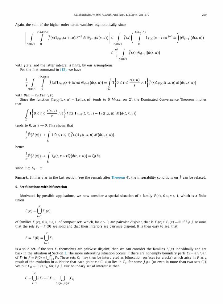
Fig. 1. The set F1 along with A(ε) = (0, ε] × [0,1] (dotted line).
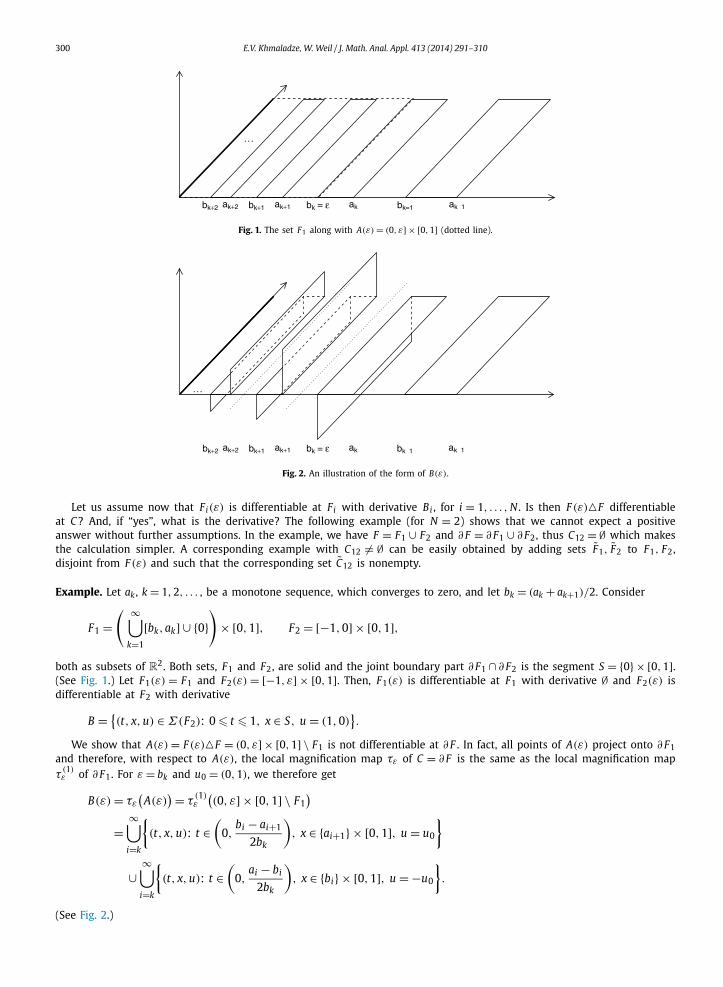
Fig. 2. An illustration of the form of B(ε).
Let us assume now that Fi(ε) is differentiable at Fi with derivative Bi , for i = 1, . . . , N . Is then F (ε)�F differentiableat C? And, if “yes”, what is the derivative? The following example (for N = 2) shows that we cannot expect a positiveanswer without further assumptions. In the example, we have F = F1 ∪ F2 and ∂ F = ∂ F1 ∪ ∂ F2, thus C12 = ∅ which makesthe calculation simpler. A corresponding example with C12 �= ∅ can be easily obtained by adding sets F1, F2 to F1, F2,disjoint from F (ε) and such that the corresponding set C12 is nonempty.
Example. Let ak , k = 1,2, . . . , be a monotone sequence, which converges to zero, and let bk = (ak + ak+1)/2. Consider
F1 =( ∞⋃
k=1
[bk,ak] ∪ {0})
× [0,1], F2 = [−1,0] × [0,1],
both as subsets of R2. Both sets, F1 and F2, are solid and the joint boundary part ∂ F1 ∩ ∂ F2 is the segment S = {0} × [0,1].(See Fig. 1.) Let F1(ε) = F1 and F2(ε) = [−1, ε] × [0,1]. Then, F1(ε) is differentiable at F1 with derivative ∅ and F2(ε) isdifferentiable at F2 with derivative
B = {(t, x, u) ∈ Σ(F2): 0 � t � 1, x ∈ S, u = (1,0)
}.
We show that A(ε) = F (ε)�F = (0, ε] × [0,1] \ F1 is not differentiable at ∂ F . In fact, all points of A(ε) project onto ∂ F1and therefore, with respect to A(ε), the local magnification map τε of C = ∂ F is the same as the local magnification mapτ
(1)ε of ∂ F1. For ε = bk and u0 = (0,1), we therefore get
B(ε) = τε
(A(ε)
) = τ(1)ε
((0, ε] × [0,1] \ F1
)=
∞⋃i=k
{(t, x, u): t ∈
(0,
bi − ai+1
2bk
), x ∈ {ai+1} × [0,1], u = u0
}
∪∞⋃
i=k
{(t, x, u): t ∈
(0,
ai − bi
2bk
), x ∈ {bi} × [0,1], u = −u0
}.
(See Fig. 2.)
E.V. Khmaladze, W. Weil / J. Math. Anal. Appl. 413 (2014) 291–310 301
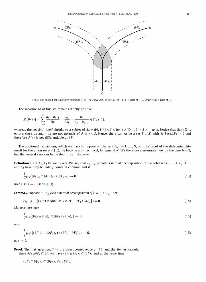
Fig. 3. The shaded set illustrates condition (13). The curve ADC is part of ∂ F1, BDC is part of ∂ F2, while ADB is part of ∂ F .
The measure M of this set remains strictly positive,
M(
B(ε)) =
∞∑i=k
ai − ai+1
2bk= ak
2bk= ak
ak + ak+1∈ [1/2,1],
whereas the set B(ε) itself shrinks to a subset of B0 = ([0,1/4] × S × {u0}) ∪ ([0,1/4] × S × {−u0}). Notice that B0 ∩ Σ isempty, since u0 and −u0 are not normals of F at x ∈ S . Hence, there cannot be a set B ⊂ Σ with M(B(ε)�B) → 0 andtherefore A(ε) is not differentiable at ∂ F .
The additional restrictions, which we have to impose on the sets Fi , i = 1, . . . , N , and the proof of the differentiabilityresult for the union set F = ⋃N
i=1 Fi become a bit technical, for general N . We therefore concentrate now on the case N = 2,but the general case can be treated in a similar way.
Definition 3. Let F1, F2 be solids sets. We say that F1, F2 provide a normal decomposition of the solid set F = F1 ∪ F2, if F1and F2 have only boundary points in common and if
1
εμd
((∂ F )ε ∩ (∂ F1)ε ∩ (∂ F2)ε
) → 0 (13)
holds, as ε → 0 (see Fig. 3).
Lemma 7. Suppose F1, F2 yield a normal decomposition of F = F1 ∪ F2 . Then
Θd−1(C,
{(x, u) ∈ Nor(C): x ∈ ∂ F ∩ ∂ F1 ∩ ∂ F2
}) = 0. (14)
Moreover, we have
1
εμd
((∂ F1�∂ F2)ε ∩ (∂ F1 ∩ ∂ F2)ε
) → 0 (15)
and
1
εμd
(((∂ F1)ε ∩ (∂ F2)ε
) \ (∂ F1 ∩ ∂ F2)ε) → 0, (16)
as ε → 0.
Proof. The first assertion, (14), is a direct consequence of (13) and the Steiner formula.Since ∂ F1�∂ F2 ⊆ ∂ F , we have (∂ F1�∂ F2)ε ⊆ (∂ F )ε and at the same time
(∂ F1 ∩ ∂ F2)ε ⊆ (∂ F1)ε ∩ (∂ F2)ε.
302 E.V. Khmaladze, W. Weil / J. Math. Anal. Appl. 413 (2014) 291–310
Therefore,
(∂ F1�∂ F2)ε ∩ (∂ F1 ∩ ∂ F2)ε ⊆ (∂ F )ε ∩ (∂ F1)ε ∩ (∂ F2)ε,
and (15) follows from condition (13).With respect to (16),
z ∈ ((∂ F1)ε ∩ (∂ F2)ε
) \ (∂ F1 ∩ ∂ F2)ε
implies that the distances d∂ F1 (z),d∂ F2 (z) do not exceed ε, but d∂ F1∩∂ F2 (z) > ε. Therefore z is on a distance smaller than orequal to ε not from ∂ F1 ∩ ∂ F2, but from ∂ F1�∂ F2, that is, from ∂ F . Hence(
(∂ F1)ε ∩ (∂ F2)ε) \ (∂ F1 ∩ ∂ F2)ε ⊆ (∂ F )ε ∩ (∂ F1)ε ∩ (∂ F2)ε
and (16) follows, again from (13). �We now discuss the normal cylinders of the sets involved. Apparently, this reduces to a discussion of the corresponding
normal bundles. The normal bundle Nor(C) of C can be embedded as a subset into the union of the normal bundlesNor(∂ Fi), i = 1,2. In fact, any (x, u) ∈ Nor(C) comes from a point z /∈ C which (uniquely) projects onto x ∈ C . If x ∈ ∂ F1,then x is also the projection of z onto ∂ F1 and hence (x, u) ∈ Nor(F1). We similarly argue if x ∈ ∂ F2.
In order to embed also Nor(∂ F1) into Nor(C), we have to neglect pairs (x1, u) from Nor(∂ F1) for which u is not a normalat x in C . For such a pair (x1, u) ∈ Nor(∂ F1), there exists small enough ε, such that all z = x1 + tu, t � ε, project onto x1.Since ∂ F1 ⊆ C , there is a point x2 ∈ C with
‖z − x2‖ = infx∈C
‖z − x‖ � infx∈∂ F1
‖z − x‖ = ‖z − x1‖,and therefore all points z = x1 + tu, t � ε, are in Cε . However, x2 has to be different from x1. Otherwise, we would have(z − x2)/‖z − x2‖ = u and (x1, u) ∈ Nor(C), a contradiction. Therefore, we obtain z ∈ (∂ F1)ε ∩ (∂ F2)ε \ Cε . Applying the localmagnification map τ
(1)ε to this set and using (16) and the Steiner formula, we deduce that
Θd−1(∂ F1,Nor(∂ F1) \ Nor(C)
) = 0,
which shows that we can embed Σ(∂ F1) into Σ(C), up to a set of measure 0. In the same way, we can embed Nor(∂ F2)
into Nor(C).Therefore, we identify now the normal cylinders Σ(C) and Σ(F1) ∪ Σ(F2). If Bi denotes the derivative of Fi(ε) at Fi ,
i = 1,2, the positive part B+i and the reflection R(B−
i ) of its negative part B−i can be seen as subsets of Σ(∂ Fi), as we
have explained before Theorem 6 and therefore also as subsets of Σ(C), for i = 1,2. Since we can also embed the normalcylinders Σ(F ) of F and Σ(Fi) of Fi , i = 1,2, into Σ = Σ(C) by the mapping (t, x, u) → (t, x, u), for t � 0, and by thereflection R : (t, x, u) → (−t, x,−u), for t < 0, we can extend the measures M F and M Fi , i = 1,2, to Σ(C), in the obviousway. We denote by M+
F , M−F the restrictions of M F to Σ+(F ) respectively Σ−(F ) and we use similar notations for the
measures M Fi , i = 1,2.
Lemma 8. Suppose F1, F2 yield a normal decomposition of F = F1 ∪ F2 . Then
MC = M+F + M−
F1◦ R + M−
F2◦ R. (17)
Proof. The assertion follows from a corresponding decomposition of the support measures,
Θd−1(C, ·) = Θd−1(F , ·) + Θd−1(
F ∗1 , ·) + Θd−1
(F ∗
2 , ·)which is a consequence of (5) and (10), together with (14). �
We now formulate our main result in this section.
Theorem 9. Let F1(ε), F2(ε), 0 � ε � 1, be two families of nonempty compact sets such that, for each fixed ε > 0, the sets F1(ε) andF2(ε) are pairwise disjoint, and let F (ε) = F1(ε) ∪ F2(ε). Assume that F1 = F1(0) and F2 = F2(0) provide a normal decompositionof F = F (0) = F1 ∪ F2 .
If the families Fi(ε) are differentiable at Fi with derivative Bi , i = 1,2, then
C(ε) = F (ε)�F
is differentiable at
C = ∂ F1 ∪ ∂ F2
E.V. Khmaladze, W. Weil / J. Math. Anal. Appl. 413 (2014) 291–310 303
with derivative B = B1 ∪ B2 where
Bi ={
R(B−i ) \ B+
j on Σ(Cij) for j �= i,
B+i ∪ R(B−
i ) otherwise.
Proof. We start with the essential boundedness condition. Since the families Fi(ε)�Fi are essentially bounded, we mayassume that there is a T such that
Fi(ε)�Fi ⊂ (∂ Fi)Tε, i = 1,2.
We may also put T = 1. It is then easy to see that
F (ε)�F ⊂ Cε,
hence C(ε) is essentially bounded.In order to show that F (ε)�F is differentiable at C with derivative B , it remains to show that
MC(τε
(F (ε)�F
)�B) → 0,
as ε → 0. Observe that here τε is the magnification map belonging to C . Later, we will also use the magnification map τ(i)ε
belonging to ∂ Fi , i = 1,2. For z /∈ C ∪ SC ∪ S∂ F1 ∪ S∂ F2 , we then have τε(z) = τ(i)ε (z), for some i (possibly for both). We now
use (17) and discuss the effects of the different summands of MC to the set τε(F (ε)�F )�B separately.Since M+
F is concentrated on [0,∞) × Nor(F ) (notice that we can use Nor(F ) instead of Nore(F ) here), we can decom-pose M+
F into a sum
M+F = M(1) + M(2),
where
M(i) = μ+1 ⊗ [
Θd−1(Fi, ·)(Nor(Fi) ∩ Nor(F )
)], i = 1,2.
Here, μ+1 is the Lebesgue measure on [0,∞) and ρ A denotes the restriction of the measure ρ to the set A. Using this
decomposition and the facts that
τε
(F (ε)�F
)�B ⊂ [τε
(F (ε) \ F
)�B] ∪ τε(F )
and M+F (τε(F )) = 0, we first obtain
M+F
(τε
(F (ε)�F
)�B)� M+
F
(τε
(F (ε) \ F
)�B)
=2∑
i=1
M(i)(τε
(F (ε) \ F
)�B).
On [0,∞) × (Nor(F1) ∩ Nor(F )), we have
τε
(F (ε) \ F
) = τ(1)ε
((F (ε) \ F
) ∩ (∂ F1)ε)
= τ(1)ε
(F1(ε) \ F1
) ∪ τ(1)ε
((F2(ε) \ F1
) ∩ (∂ F1)ε),
hence
M(1)(τε
(F (ε) \ F
)�B)� M(1)
(τ
(1)ε
(F1(ε) \ F1
)�B) + M(1)
(τ
(1)ε
((F2(ε) \ F1
) ∩ (∂ F1)ε))
. (18)
Moreover,
M(1)(
B+2
) = M(1)(
R(
B−2
)) = M(1)(
B−1
) = M(1)(
R(
B−1
)) = 0
(the latter fact arises, since Nor(F1) and R(B−1 ) are disjoint subsets of Nor(C)). Therefore,
M(1)(τ
(1)ε
(F1(ε) \ F1
)�B) = M(1)
(τ
(1)ε
(F1(ε) \ F1
)�B+1
)= M(1)
(τ
(1)ε
(F1(ε)�F1
)�B+1
)= M(1)
(τ
(1)ε
(F1(ε)�F1
)�B1).
Since M(1) � M F1 , we get
304 E.V. Khmaladze, W. Weil / J. Math. Anal. Appl. 413 (2014) 291–310
M(1)(τ
(1)ε
(F1(ε) \ F1
)�B)� M F1
(τ
(1)ε
(F1(ε)�F1
)�B1) → 0, (19)
as ε → 0, due to the differentiability of F1(ε).Furthermore, we notice that points z in (F2(ε) \ F1) ∩ (∂ F1)ε which project onto ∂ F1 must lie in (∂ F1 \ ∂ F2)ε ∩ (∂ F1 ∩
∂ F2)ε , and so
M(1)(τ
(1)ε
((F2(ε) \ F1
) ∩ (∂ F1)ε))
� M(1)(τ
(1)ε
((∂ F1 \ ∂ F2)ε ∩ (∂ F1 ∩ ∂ F2)ε
)).
The local Steiner formula (2) shows that
1
εμd
((∂ F1 \ ∂ F2)ε ∩ (∂ F1 ∩ ∂ F2)ε
) = M(1)(τ
(1)ε
((∂ F1 \ ∂ F2)ε ∩ (∂ F1 ∩ ∂ F2)ε
)) + o(ε).
Therefore, (15) implies
M(1)(τ
(1)ε
((∂ F1 \ ∂ F2)ε ∩ (∂ F1 ∩ ∂ F2)ε
)) → 0, (20)
as ε → 0. Combining (18), (19) and (20) gives
M(1)(τε
(F (ε) \ F
)�B) → 0.
In the same way, we get
M(2)(τε
(F (ε) \ F
)�B) → 0,
hence
M+F
(τε
(F (ε)�F
)�B) → 0. (21)
Now, we consider(M−
F1◦ R
)(τε
(F (ε)�F
)�B).
Observe that M F1 = M−F1
◦ R is a measure on R(Σ−(F1)). On this set, we have
τε
(F (ε)�F
) = τ(1)ε
(F1 \ F (ε)
)= [
τ(1)ε
(F1 \ F (ε)
) ∩ Σ(F )] ∪ [
τ(1)ε
(F1 \ F (ε)
) ∩ Σ12],
here Σ12 = [0,∞) × (Nor(∂ F1) \ Nor(F )) is the normal cylinder of C12 in relative interior points of C12 and with normals upointing into the interior of F1. Notice that the sets τ
(1)ε ((F1 \ F (ε)) ∩ Σ(F )) and τ
(1)ε ((F1 \ F (ε)) ∩ Σ12) live on different
parts of the cylinder Σ(C). Therefore,
M F1
(τε
(F (ε)�F
)�B) = M F1
((τ
(1)ε
(F1 \ F (ε)
) ∩ Σ(F ))�(
R(
B−1
) ∩ Σ(F )))
+ M F1
((τ
(1)ε
(F1 \ F (ε)
) ∩ Σ12)�((
B+2 ∪ R
(B−
1
)) ∩ Σ12))
= M(1)(τ
(1)ε
(F1 \ F (ε)
)�R(
B−1
)) + M(2)(τ
(1)ε
(F1 \ F (ε)
)�(B+
2 ∪ R(
B−1
))). (22)
Here, M(1) denotes the restriction of M F1 to Σ(F ) and M(2) is the restriction to Σ12.For the first summand, we use
τ(1)ε
(F1 \ F (ε)
) = τ(1)ε
(F1 \ F1(ε)
) \ τ(1)ε
(F1 ∩ F2(ε)
)and
M(1)(τ
(1)ε
(F1 \ F1(ε)
)�R(
B−1
)) → 0,
since F1(ε) is differentiable at F1. Also
M(1)(τ
(1)ε
(F1 ∩ F2(ε)
)) → 0. (23)
In fact, the Steiner formula (2) shows that
M(1)(τ
(1)ε
(F1 ∩ F2(ε)
)) = 1
εμd
((∂ F1)ε ∩ (
F1 ∩ F2(ε))) + o(ε).
Points z ∈ (∂ F1)ε ∩ (F1 ∩ F2(ε)) which project onto ∂ F lie in (∂ F1)ε ∩ (∂ F2)ε ∩ (∂ F )ε . Hence, the assertion follows from (13).

E.V. Khmaladze, W. Weil / J. Math. Anal. Appl. 413 (2014) 291–310 305
Together we get
M(1)(τ
(1)ε
(F1 \ F (ε)
)�R(
B−1
)) → 0. (24)
For the second summand in (22), we similarly have
τ(1)ε
(F1 \ F (ε)
) = τ(1)ε
(F1 \ F1(ε)
) \ τ(1)ε
(F1 ∩ F2(ε)
)with
M(2)(τ
(1)ε
(F1 \ F1(ε)
)�R(
B−1
)) → 0,
again by the differentiability of F1(ε). On the other hand,
M(2)(τ
(1)ε
(F1 ∩ F2(ε)
)) = M F1
(τ
(1)ε
((F1 ∩ F2(ε)
) ∩ Σ12))
= M+F2
(τ
(2)ε
(F1 ∩ F2(ε)
) ∩ Σ12) − M F1
(τ
(1)ε
(F1 ∩ F2(ε)
) ∩ Σ(F )),
taking into account the points in F1 ∩ F2(ε) which project onto ∂ F and not onto C12. Here,
M+F2
((τ
(2)ε
(F1 ∩ F2(ε)
) ∩ Σ12)�(
B+2 ∩ Σ12
)) → 0,
by the differentiability of F2(ε) and the term
M F1
(τ
(1)ε
(F1 ∩ F2(ε)
) ∩ Σ(F ))
converges to 0 by our condition (13), as we have seen in (23). Hence,
M(2)(τ
(1)ε
(F1 ∩ F2(ε)
)�B+2
) → 0.
Together we obtain
M(2)(τ
(1)ε
(F1 \ F (ε)
)�(R(
B−1
) \ B+2
))= M(2)
(τ
(1)ε
(F1 \ F1(ε)
)�τ(1)ε
(F1 ∩ F2(ε)
)�(R(
B−1
)�B+2
))� M(2)
(τ
(1)ε
(F1 \ F1(ε)
)�R(
B−1
)) + M(2)(τ
(1)ε
(F1 ∩ F2(ε)
)�B+2
) → 0. (25)
From (24) and (25), we arrive at
(M−
F1◦ R
)(τε
(F�F (ε)
)�B) → 0. (26)
In the same manner, we get
(M−
F2◦ R
)(τε
(F�F (ε)
)�B) → 0. (27)
Combining (21), (26) and (27), we obtain the asserted differentiability. �6. Parallel sets
We now discuss some particular classes of set-valued mappings which are differentiable, the subgraphs and the local orglobal parallel sets.
Let F = F (0) be a solid set and hε , 0 � ε � 1, a family of nonnegative measurable functions on Nor(F ) (with h0 = 0). Asin [9], we call
hε,sub = {z = x + tu: (x, u) ∈ Nor(F ), 0 < t � hε(x, u) ∧ r(x, u)
}the subgraph of hε . We assume that the following two conditions hold:
(a) For each (x, u) ∈ Nor(F ), ε → hε(x, u) is differentiable at ε = 0 with derivative g(x, u). Thus
hε(x, u)
ε→ g(x, u), ε → 0.
306 E.V. Khmaladze, W. Weil / J. Math. Anal. Appl. 413 (2014) 291–310
(b) There is a δ > 0, such that the function max0<ε�δhεε is bounded and integrable with respect to Θd−1(F , ·). Hence,
max0<ε�δ
hε(x, u)
ε� T , (28)
for some T > 0 and∫Nor(F )
max0<ε�δ
hε(x, u)
εΘd−1
(F ,d(x, u)
)< ∞.
Theorem 10. Let F be solid and let hε , 0 � ε � 1, be a family of nonnegative measurable functions on Nor(F ) satisfying conditions (a)and (b). Then, A(ε) = hε,sub is differentiable at ∂ F and the derivative is
B = {(t, x, u): 0 < t � g(x, u), (x, u) ∈ Nor(F )
}.
Proof. We first show that A(ε) is essentially bounded. Let δ be given as in (b) and let T be the bound from (28). Supposeε � δ. Then,
1
εμd
(A(ε) ∩ (
Rd \ (∂ F )εT)) = 1
εμd
({z = x + tu: (x, u) ∈ Nor(F ), εT < t � hε(x, u) ∧ r(x, u)
})equals 0, because condition (b) implies that the set here is empty. Hence, A(ε) is essentially bounded.
With respect to the differentiability, we observe that
M(τε
(A(ε)
)�B) =
∫Nor(F )
∞∫0
1({
0 < t � hε(x, u) ∧ r(x, u)
ε
}�{
0 < t � g(x, u)})
dt Θd−1(
F ,d(x, u))
=∫
Nor(F )
∣∣∣∣hε(x, u) ∧ r(x, u)
ε− g(x, u)
∣∣∣∣Θd−1(
F ,d(x, u)).
Since r(x, u) > 0, for (x, u) ∈ Nor(F ), the integrand converges to 0 pointwise. Also,∣∣∣∣hε(x, u) ∧ r(x, u)
ε− g(x, u)
∣∣∣∣ � hε(x, u) ∧ r(x, u)
ε+ g(x, u)
� 2 max0<ε�δ
hε(x, u)
ε,
and the latter function is integrable with respect to Θd−1(F , ·), by (b). The Dominated Convergence Theorem thus implies
M(
F (ε)�B) → 0, ε → 0.
This completes the proof of the theorem. �We remark that we could also start with a family hε , 0 < ε � 1, of functions on ∂ F and put hε(x, u) = hε(x), (x, u) ∈
Nor(F ), or with a family hε , 0 < ε � 1, of functions on Sd−1 and put hε(x, u) = hε(u), (x, u) ∈ Nor(F ).As a particular case, hε = εg and the function g could be given by the support function hK of a convex body K with
0 ∈ K ,
g(x, u) = hK (u), (x, u) ∈ Nor(F ).
The subgraph hε,sub, obtained in this case, is different in general from the outer parallel strip F + εK \ F . A differentiabilityresult for outer parallel sets F + εK , ε → 0, under different conditions, is discussed in Theorem 12 below. However, if K isthe unit ball Bd and
hε(x, u) = εhBd (u) = ε,
then hε,sub = F + εBd \ F , as can be easily seen.A case of particular interest arises, if we choose, in the previous discussion, h(x, u) = r(x, u) ∧ 1, (x, u) ∈ Nor(F ). If we
define, for ε > 0, the local parallel set Fε,loc of F as
Fε,loc = F ∪ {z = x + tu: (x, u) ∈ Nor F , 0 < t � εr(x, u) ∧ ε
},
E.V. Khmaladze, W. Weil / J. Math. Anal. Appl. 413 (2014) 291–310 307
then Fε,loc is the subgraph of εh. The derivative of εh is r ∧ 1, hence in the above proof we have
M(τε
(A(ε)
)�B) =
∫Nor(F )
∣∣∣∣hε(x, u) ∧ r(x, u)
ε− g(x, u)
∣∣∣∣Θd−1(
F ,d(x, u))
=∫
Nor(F )
∣∣∣∣ε(r(x, u) ∧ 1) ∧ r(x, u)
ε− (
r(x, u) ∧ 1)∣∣∣∣Θd−1
(F ,d(x, u)
)
= 0,
for ε � 1. Condition (b) is satisfied automatically since r ∧ 1 is bounded and integrable with respect to Θd−1(F , ·) by (1).Hence, we obtain the following result.
Corollary 11. Let F be a solid set. Then the local parallel set Fε,loc , 0 < ε � 1, is differentiable at F with derivative
B = {(t, x, u): (x, u) ∈ Nor(F ), 0 � t � r(x, u) ∧ 1
}.
As a consequence, the parallel set F + εBd of a convex body F is differentiable, as we already mentioned above. This isa special case of a result in [9] which shows differentiability of F + εK , for general convex bodies F , K . Our next goal is toextend the latter result to solid sets F .
For this purpose, we consider the support function hK of K ; it can be seen as a continuous function on Sd−1. We definea function hK ,F on Nor(F ) by
hK ,F (x, u) = hK (u), (x, u) ∈ Nor(F ),
and put
(hK ,F )sub = {(t, x, u) ∈ Σ: 0 < t � hK (u)
} ∪ {(t, x, u) ∈ Σ: hK (u) � t < 0
}.
Notice, that we do not require 0 ∈ K here. This is another difference to the discussion of subgraphs above.In the following theorem, we assume, in addition, that the support measure Θd−1(F , ·) is finite (this follows, for ex-
ample, if ∂ F has finite (d − 1)-st Hausdorff measure) and that the set of boundary points of F which are not normal hasHd−1-measure 0. Here, a point x ∈ ∂ F is called normal, if there is some ball B ⊂ F with x ∈ B .
Theorem 12. Let F be a solid set with Θd−1(F ,Nor(F )) < ∞ and such that
Hd−1({x ∈ ∂ F : x not normal}) = 0.
Let K be a convex body. Then F (ε) = F + εK , 0 � ε � 1, is differentiable at F , and we have
d
dεF (ε) = (hK ,F )sub.
Proof. For k = 1,2, . . . , let ∂ F(k) be the set of all regular boundary points x of F for which there is a ball of radius � 1/kinside F with x ∈ B . Let u = u(x) be the corresponding (outer) normal. Let Σ(k) ⊂ Σ be the part of the normal cylinderwhich belongs to points (x, u(x)), x ∈ ∂ F(k) . We fix k and choose ε small enough such that εK ⊂ 1
k Bd . Then, we consider
M([
τε
(F (ε)�F
)�(hK ,F )sub] ∩ Σ(k)
).
For x ∈ ∂ F(k) (with normal u), we have B(1/k) ⊂ F ⊂ H(x, u), where B(1/k) is the ball of radius 1/k touching F at x frominside. H(x, u) is the closure of the complement Rd \ C , where C is the ball of radius r(x, u) touching F in x from outside.If the reach r(x, u) is ∞, then H(x, u) is the closed halfspace with outer normal u and containing x in the boundary. Wedivide Σ(k) further into the sets Σ+
(k)and Σ−
(k)according to the case where hK ,F (x, u) � 0, respectively hK ,F (x, u) < 0.
Since εK ⊂ 1k Bd , we have[
τε
(F (ε)�F
)�(hK ,F )sub] ∩ Σ+
(k)= [
τε
(F (ε) \ F
)�(hK ,F )sub] ∩ Σ+
(k)
and
τε
(F (ε) \ F
) ∩ Σ+(k)
={(
t, x, u
): 0 < t � gεK (x, u)
},
ε
308 E.V. Khmaladze, W. Weil / J. Math. Anal. Appl. 413 (2014) 291–310
where gεK (x, u) is the distance from x to ∂ F (ε) in direction u. For F = H(x, u) this distance would be εhK (u), for F = B(1/k)
the distance is � εhK (u) +√
(1/k)2 − ε2(a(u)2 − h2K (u)) − 1/k, where a(u) is the maximal length of a point y ∈ K with
〈y, u〉 = hK (u). Hence
εhK (u) +√
1
k2− ε2
(a(u)2 − h2
K (u)) − 1
k� gεK (x, u) � εhK (u).
We obtain that
[τε
(F (ε) \ F
)�(hK ,F )sub] ∩ Σ(k) ⊂
{(t, x, u): hK (u) + 1
ε
(√1
k2− ε2
(a(u)2 − h2
K (u)) − 1
k
)� t � hK (u)
}.
Since
limε→0
1
ε
(√1
k2− ε2
(a(u)2 − h2
K (u)) − 1
k
)= 0,
we see that
M([
τε
(F (ε) \ F
)�(hK ,F )sub] ∩ Σ+
(k)
) → 0.
In a totally analogous way, we obtain that[τε
(F (ε)�F
)�(hK ,F )sub] ∩ Σ−
(k)= [
τε
(F \ F (ε)
)�(hK ,F )sub] ∩ Σ−
(k)
and
M([
τε
(F \ F (ε)
)�(hK ,F )sub] ∩ Σ−
(k)
) → 0.
Hence,
M([
τε
(F�F (ε)
)�(hK ,F )sub] ∩ Σ(k)
) → 0,
for each k, and therefore also
M(τε
(F (ε) \ F
)�(hK ,F )sub) → 0,
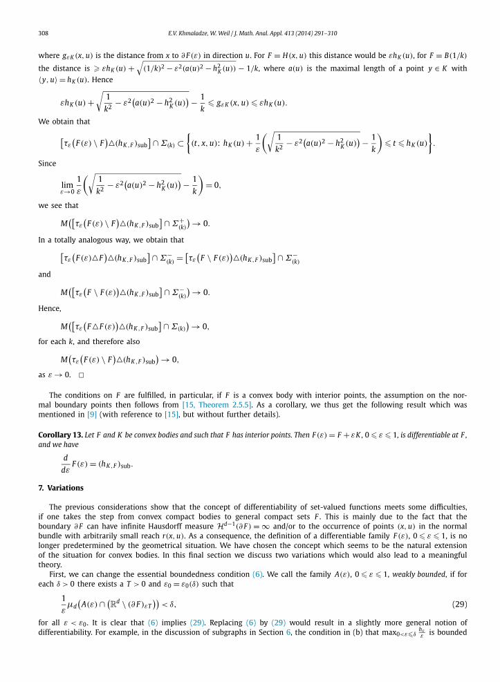
as ε → 0. �The conditions on F are fulfilled, in particular, if F is a convex body with interior points, the assumption on the nor-
mal boundary points then follows from [15, Theorem 2.5.5]. As a corollary, we thus get the following result which wasmentioned in [9] (with reference to [15], but without further details).
Corollary 13. Let F and K be convex bodies and such that F has interior points. Then F (ε) = F + εK , 0 � ε � 1, is differentiable at F ,and we have
d
dεF (ε) = (hK ,F )sub.
7. Variations
The previous considerations show that the concept of differentiability of set-valued functions meets some difficulties,if one takes the step from convex compact bodies to general compact sets F . This is mainly due to the fact that theboundary ∂ F can have infinite Hausdorff measure Hd−1(∂ F ) = ∞ and/or to the occurrence of points (x, u) in the normalbundle with arbitrarily small reach r(x, u). As a consequence, the definition of a differentiable family F (ε), 0 � ε � 1, is nolonger predetermined by the geometrical situation. We have chosen the concept which seems to be the natural extensionof the situation for convex bodies. In this final section we discuss two variations which would also lead to a meaningfultheory.
First, we can change the essential boundedness condition (6). We call the family A(ε), 0 � ε � 1, weakly bounded, if foreach δ > 0 there exists a T > 0 and ε0 = ε0(δ) such that
1
εμd
(A(ε) ∩ (
Rd \ (∂ F )εT))
< δ, (29)
for all ε < ε0. It is clear that (6) implies (29). Replacing (6) by (29) would result in a slightly more general notion ofdifferentiability. For example, in the discussion of subgraphs in Section 6, the condition in (b) that max0<ε�δ
hε is bounded
ε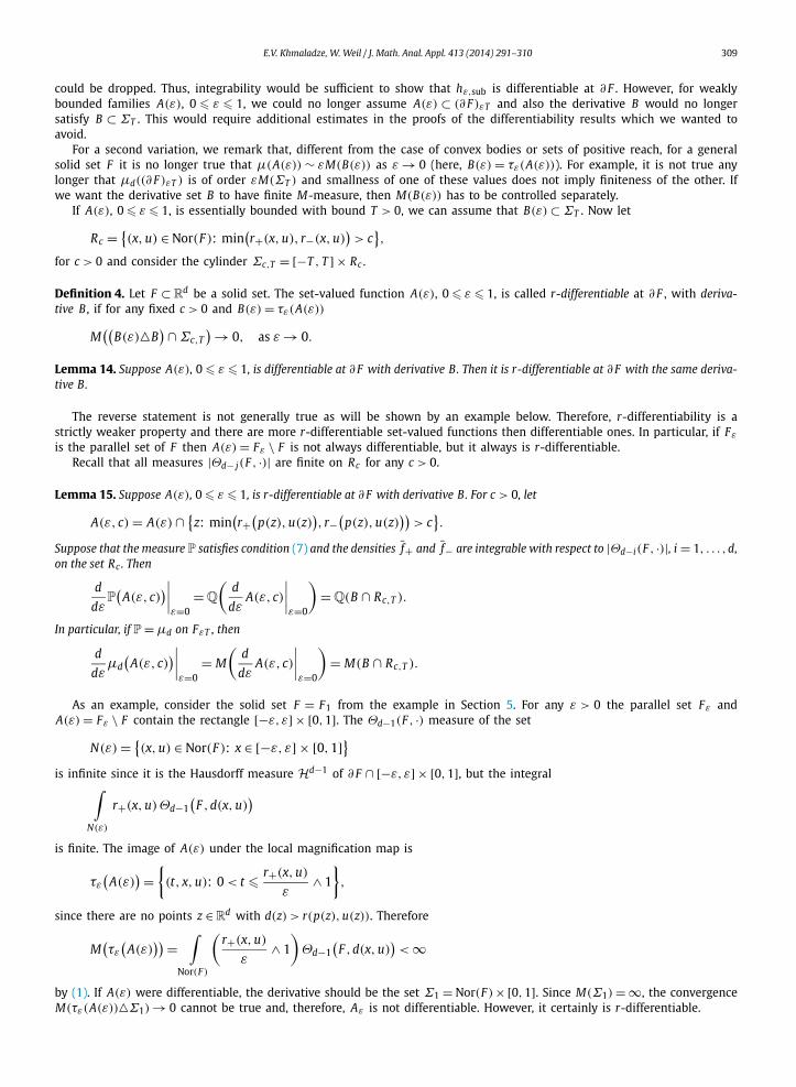
E.V. Khmaladze, W. Weil / J. Math. Anal. Appl. 413 (2014) 291–310 309
could be dropped. Thus, integrability would be sufficient to show that hε,sub is differentiable at ∂ F . However, for weaklybounded families A(ε), 0 � ε � 1, we could no longer assume A(ε) ⊂ (∂ F )εT and also the derivative B would no longersatisfy B ⊂ ΣT . This would require additional estimates in the proofs of the differentiability results which we wanted toavoid.
For a second variation, we remark that, different from the case of convex bodies or sets of positive reach, for a generalsolid set F it is no longer true that μ(A(ε)) ∼ εM(B(ε)) as ε → 0 (here, B(ε) = τε(A(ε))). For example, it is not true anylonger that μd((∂ F )εT ) is of order εM(ΣT ) and smallness of one of these values does not imply finiteness of the other. Ifwe want the derivative set B to have finite M-measure, then M(B(ε)) has to be controlled separately.
If A(ε), 0 � ε � 1, is essentially bounded with bound T > 0, we can assume that B(ε) ⊂ ΣT . Now let
Rc = {(x, u) ∈ Nor(F ): min
(r+(x, u), r−(x, u)
)> c
},
for c > 0 and consider the cylinder Σc,T = [−T , T ] × Rc .
Definition 4. Let F ⊂ Rd be a solid set. The set-valued function A(ε), 0 � ε � 1, is called r-differentiable at ∂ F , with deriva-tive B , if for any fixed c > 0 and B(ε) = τε(A(ε))
M((
B(ε)�B) ∩ Σc,T
) → 0, as ε → 0.
Lemma 14. Suppose A(ε), 0 � ε � 1, is differentiable at ∂ F with derivative B. Then it is r-differentiable at ∂ F with the same deriva-tive B.
The reverse statement is not generally true as will be shown by an example below. Therefore, r-differentiability is astrictly weaker property and there are more r-differentiable set-valued functions then differentiable ones. In particular, if Fε
is the parallel set of F then A(ε) = Fε \ F is not always differentiable, but it always is r-differentiable.Recall that all measures |Θd− j(F , ·)| are finite on Rc for any c > 0.
Lemma 15. Suppose A(ε), 0 � ε � 1, is r-differentiable at ∂ F with derivative B. For c > 0, let
A(ε, c) = A(ε) ∩ {z: min
(r+
(p(z), u(z)
), r−
(p(z), u(z)
))> c
}.
Suppose that the measure P satisfies condition (7) and the densities f+ and f− are integrable with respect to |Θd−i(F , ·)|, i = 1, . . . ,d,on the set Rc . Then
d
dεP(
A(ε, c))∣∣∣∣
ε=0= Q
(d
dεA(ε, c)
∣∣∣∣ε=0
)= Q(B ∩ Rc,T ).
In particular, if P = μd on FεT , then
d
dεμd
(A(ε, c)
)∣∣∣∣ε=0
= M
(d
dεA(ε, c)
∣∣∣∣ε=0
)= M(B ∩ Rc,T ).
As an example, consider the solid set F = F1 from the example in Section 5. For any ε > 0 the parallel set Fε andA(ε) = Fε \ F contain the rectangle [−ε, ε] × [0,1]. The Θd−1(F , ·) measure of the set
N(ε) = {(x, u) ∈ Nor(F ): x ∈ [−ε, ε] × [0,1]}
is infinite since it is the Hausdorff measure Hd−1 of ∂ F ∩ [−ε, ε] × [0,1], but the integral∫N(ε)
r+(x, u)Θd−1(
F ,d(x, u))
is finite. The image of A(ε) under the local magnification map is
τε
(A(ε)
) ={(t, x, u): 0 < t � r+(x, u)
ε∧ 1
},
since there are no points z ∈Rd with d(z) > r(p(z), u(z)). Therefore
M(τε
(A(ε)
)) =∫
Nor(F )
(r+(x, u)
ε∧ 1
)Θd−1
(F ,d(x, u)
)< ∞
by (1). If A(ε) were differentiable, the derivative should be the set Σ1 = Nor(F )×[0,1]. Since M(Σ1) = ∞, the convergenceM(τε(A(ε))�Σ1) → 0 cannot be true and, therefore, Aε is not differentiable. However, it certainly is r-differentiable.

310 E.V. Khmaladze, W. Weil / J. Math. Anal. Appl. 413 (2014) 291–310
References
[1] Z. Artstein, A calculus of set-valued maps and set-valued evolution equations, Set-Valued Anal. 3 (1995) 213–261.[2] J.-P. Aubin, H. Frankowska, Set-Valued Analysis, Birkhäuser, Basel, 1990.[3] J.M. Borwein, Q.J. Zhu, A survey of sub-differential calculus with applications, Nonlinear Anal. 38 (1999) 687–773.[4] B.E. Brodsky, B.S. Darkhovsky, Nonparametric Methods in Change-Point Problems, Kluwer Acad. Publishers, Dordrecht, 1993.[5] E. Carlstein, H.-G. Müller, D. Siegmund (Eds.), Change-Point Problems, IMS Lecture Notes Monogr. Ser., vol. 23, Inst. Math. Statist., Hayward, 1994.[6] J.H.J. Einmahl, E. Khmaladze, Central limit theorems for local empirical processes near boundaries of sets, Bernoulli 17 (2011) 545–561.[7] D. Hug, G. Last, W. Weil, A local Steiner-type formula for general closed sets and applications, Math. Z. 246 (2004) 237–272.[8] B.G. Ivanoff, E. Merzbach, Optimal detection of a change-set in a spatial Poisson process, Ann. Appl. Probab. 20 (2010) 640–659.[9] E. Khmaladze, Differentiation of sets in measure, J. Math. Anal. Appl. 334 (2007) 1055–1072.
[10] E. Khmaladze, R. Mnatsakanov, N. Toronjadze, The change-set problem for Vapnik–Cervonenkis classes, Math. Methods Statist. 15 (2006) 224–231.[11] E. Khmaladze, R. Mnatsakanov, N. Toronjadze, The change-set problem and local covering numbers, Math. Methods Statist. 15 (2006) 289–308.[12] E. Khmaladze, W. Weil, Local empirical processes near boundaries of convex bodies, Ann. Inst. Statist. Math. 60 (2008) 813–842.[13] A.P. Korostelev, A.B. Tsybakov, Minimax Theory of Image Reconstructions, Lecture Notes in Statist., vol. 82, Springer, New York, 1993.[14] C. Lemaréchal, J. Zowe, The eclipsing concept to approximate a multi-valued mapping, Optimization 22 (1991) 3–37.[15] R. Schneider, Convex Bodies: The Brunn–Minkowski Theory, Encyclopedia Math. Appl., vol. 44, Cambridge University Press, Cambridge, 1993.