저 시-비 리- 경 지 2.0 한민

는 아래 조건 르는 경 에 한하여 게

l 저 물 복제, 포, 전송, 전시, 공연 송할 수 습니다.

다 과 같 조건 라야 합니다:

l 하는, 저 물 나 포 경 , 저 물에 적 된 허락조건 명확하게 나타내어야 합니다.

l 저 터 허가를 면 러한 조건들 적 되지 않습니다.

저 에 른 리는 내 에 하여 향 지 않습니다.

것 허락규약(Legal Code) 해하 쉽게 약한 것 니다.

Disclaimer

저 시. 하는 원저 를 시하여야 합니다.

비 리. 하는 저 물 리 목적 할 수 없습니다.

경 지. 하는 저 물 개 , 형 또는 가공할 수 없습니다.

i

공학박사학위논문

비선형 계획법 및 모터 토크 분배를 사용한

직렬형 하이브리드 버스의 에너지 관리 전략

Energy Management Strategy of Series Hybrid Electric Bus Using

Nonlinear Programming and Motor Torque Distribution

2014 년 8 월

서울대학교 대학원

기계항공공학부

김 민 재

ii

비선형 계획법 및 모터 토크 분배를 사용한

직렬형 하이브리드 버스의 에너지 관리 전략

Energy Management Strategy of Series Hybrid Electric Bus Using

Nonlinear Programming and Motor Torque Distribution

지도교수 민 경 덕

이 논문을 공학박사 학위논문으로 제출함

2014 년 7 월

서울대학교 대학원

기계항공공학부

김 민 재

김민재의 공학박사 학위논문을 인준함

2014 년 7 월

위 원 장 : ______차__석__원______

부위원장 : ______민__경__덕______

위 원 : ______송__한__호______

위 원 : ______이__동__준______

위 원 : ______박__영__일______

iii

Abstract

Energy Management Strategy of Series Hybrid

Electric Bus Using Nonlinear Programming and

Motor Torque Distribution

Minjae Kim

Department of Mechanical and Aerospace Engineering

The Graduate School

Seoul National University

One of the most widespread issues with the hybrid electric vehicle is the

energy management strategy from the engine to the motor for fuel economy

improvement. There are lots of approaches to achieve it, but many of them are

hard to apply and/or the mathematical background is so complicated.

Furthermore, the sophisticated and complicated strategy usually required an

ideal model and environment that the practical application was not available.

Therefore, simple rule based strategies are often in use for the real-time

applications. Such a tendency was evident in SHEV (Series Hybrid Electric

Vehicle) because the structure of SHEV is so simple that those rule based

strategies such as thermostat and power follower strategies are considered to be

enough for covering the energy flow management from the engine to the battery

[1-3].

iv

This research proposes an advanced strategy which overcomes those

weaknesses. The strategy proposed in this research fully optimizes the SHEV

energy applicable to SHEV that the efficiency of the total system increase by

finding the most efficient operating points in each component in the vehicle. The

proposed strategy, which uses a semi MPC framework, has its foundation on

NLP (Nonlinear Programming) for finding minimum fuel consumption and the

speed prediction with intra-city bus was evaluated with the real bus data for the

future path plan. Furthermore, the manipulation of command signal (signal

synchronization, signal bundling, signal removing & filling up, and zero speed

synchronization) and the traction torque distribution in TMU (Traction Motor

Unit) were also considered, where the torque distribution made it possible avoid

large currents from the battery to the motor during the periods of high loading

required in the traction. The performance of the proposed strategy was compared

to that of other strategies such as DP (Dynamic Programming), thermostatic

strategy, and power follower strategy where DP gives the reference global

optimal operating points and thermostat & power follower strategies are the

well-known real-time energy distribution strategy. So, the contribution of the

proposed techniques could be evaluated.

As a result, the proposed strategy in this paper shows much better fuel

economy with the practical, fast, and exact methodology uniquely adapted to

series type hybrid electric intra-city bus. All simulation was achieved based on

AMEsim and Simulink co-simulation for the non-analytic forward bus model

and NLP solver of ‘NPSOL’ was used for the simulation.

Keywords: Diesel driven generators, Energy management, Optimal control,

Power generation control, Real time systems, Series Hybrid Electric Vehicle.

v

Student Number: 2010-30182

vi

Chapter 1. Introduction ........................................................1

1.1 Motivation ....................................................................................... 1

1.2 Literature Review ........................................................................... 7

1.3 Objectives ...................................................................................... 12

1.4 Contributions ................................................................................ 13

Chapter 2. Hybrid Electric Vehicle Modeling .................... 15

2.1 Hybrid Electric Vehicle Structure ................................................ 15

2.1.1 Series Type Structure .......................................................................... 17

2.1.2 Parallel Type Structure ........................................................................ 17

2.1.3 Series-Parallel Type Structure ............................................................. 18

2.2 Powertrain Modeling .................................................................... 23

Chapter 3. Existing Strategies ............................................ 31

3.1 Thermostat Strategy ..................................................................... 31

3.2 Power Follower Strategy............................................................... 34

3.3 Merits and Demerits of Existing Strategies ................................. 37

Chapter 4. Proposed Strategy ............................................. 39

4.1 Overall Concept ............................................................................ 39

4.2 Semi Model Predictive Control .................................................... 42

vii

4.2.1 Variables and Objective ...................................................................... 42

4.2.2 Dynamic Programming ....................................................................... 45

4.2.3 Semi Model Predictive Control ........................................................... 47

4.3 Nonlinear Programming ............................................................... 52

4.3.1 Unconstrained Optimization ............................................................... 52

4.3.2 Equality Constraints............................................................................ 53

4.3.3 Inequality Constrains .......................................................................... 54

4.3.4 SQP (Sequential Quadratic Programming) .......................................... 54

4.3.5 Problem Reconstruction ...................................................................... 54

4.3.6 NLP Starting Point Selections ............................................................. 56

4.4 Future Path Plan ........................................................................... 59

4.4.1 Bus Route ........................................................................................... 59

4.4.2 Speed Prediction Algorithm ................................................................ 62

4.4.3 Wrong Speed Prediction Handling ...................................................... 63

4.5 Signal Manipulation ..................................................................... 66

4.5.1 Signal Synchronization ....................................................................... 66

4.5.2 Signal Bundling .................................................................................. 68

4.5.3 Signal Removing and Filling Up ......................................................... 70

4.5.4 Zero Speed Synchronization ............................................................... 73

4.6 Motor Torque Distribution in MCU ............................................. 74

4.6.1 Existing Strategy ................................................................................ 74

4.6.2 Strategy Concept ................................................................................ 74

4.6.3 Procedure ........................................................................................... 76

Chapter 5. Simulation Results ............................................ 82

viii

5.1 Engine Generating Power ............................................................. 82

5.2 Battery SoC (State of Charge) ...................................................... 88

5.3 Signal Manipulations .................................................................... 90

5.4 Optimal Torque Distribution ........................................................ 93

5.5 Mode Comparisons ..................................................................... 101

5.6 Fuel Economy Comparison ........................................................ 104

Chapter 6. Conclusions ..................................................... 106

Bibliography ...................................................................... 108

초 록 .......................................................................... 117

ix

List of Tables

Table 1.1 Research Groups Currently Active in HEV Energy Control .............. 11

Table 2.1 Bus Specification ............................................................................. 27

x

List of Figures

Figure 1.1 Global Mean Land-ocean Temperature Change................................. 1

Figure 1.2 1997 Fuel Economy Statistics for Various US Models ...................... 5

Figure 1.3 ExxonMobil's Report about the Share of HEV - Main Increase of

HEVs Due to Government Policies ................................................... 6

Figure 1.4 Number of Papers in the IEEE Database of the Key Words, Hybrid

Vehicle .......................................................................................... 10

Figure 1.5 Optimization Flow (a) Engine to Battery (b) Battery to Motor (c)

Totality ......................................................................................... 15

Figure 2.1 HEV Powertrain Connection of Two Energy Sources...................... 19

Figure 2.2 Series Type Hybrid Electric Vehicle................................................ 20

Figure 2.3 Parallel Type Hybrid Electric Vehicle ............................................. 21

Figure 2.4 Series Parallel Type Hybrid Electric Vehicle ................................... 22

Figure 2.5 Simulation Model ........................................................................... 28

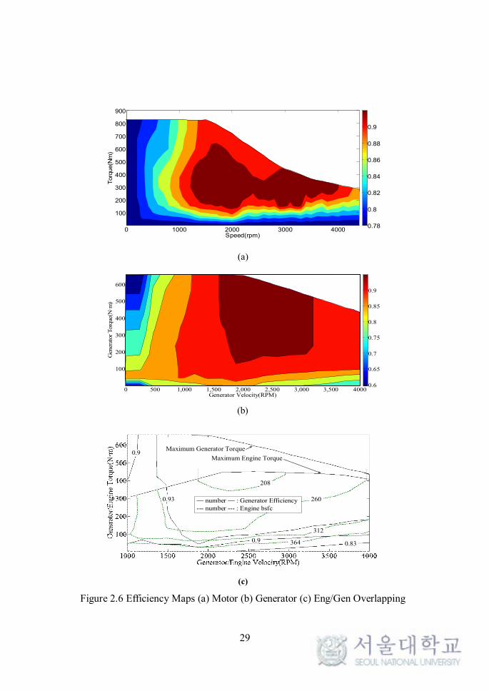
Figure 2.6 Efficiency Maps (a) Motor (b) Generator (c) Eng/Gen Overlapping 29

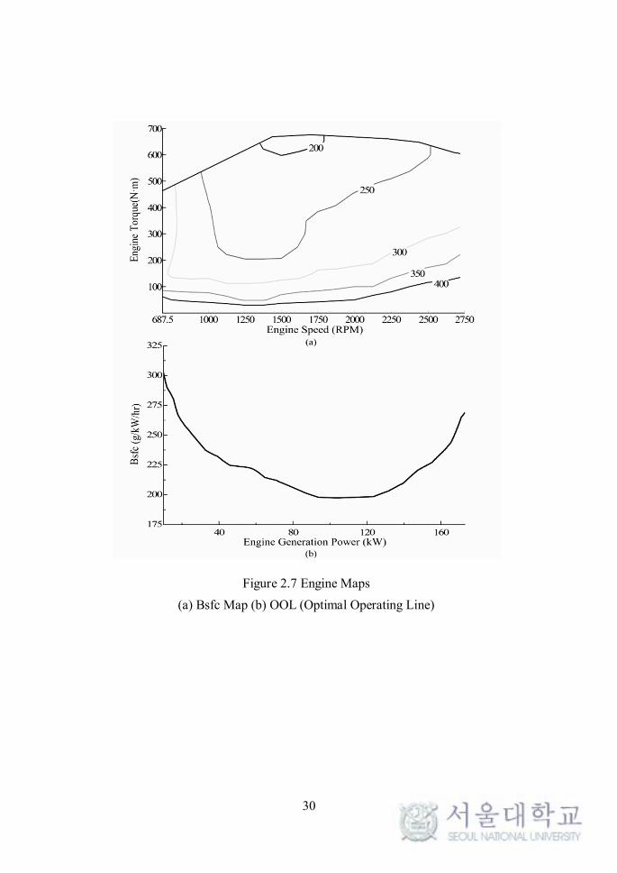
Figure 2.7 Engine Maps .................................................................................. 30

Figure 3.1 Typical Thermostat Strategy SOC Trajectory .................................. 33

xi

Figure 3.2 Power Follower Strategy Character ................................................ 36

Figure 3.3 Battery Thevenin’s equivalent circuit .............................................. 38

Figure 4.1 Algorithm Relationship .................................................................. 40

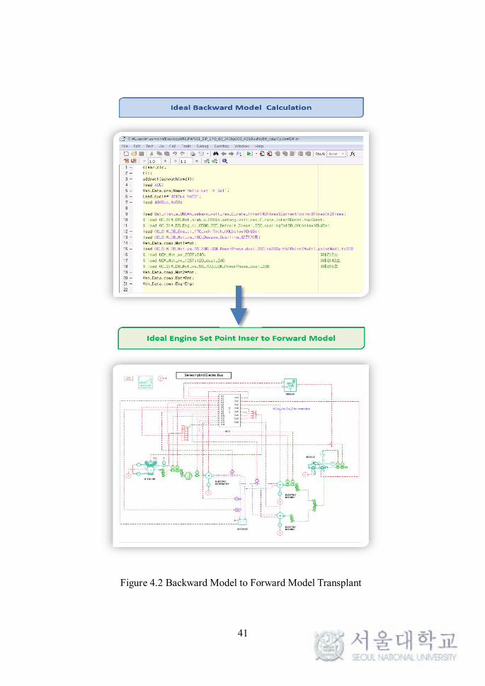
Figure 4.2 Backward Model to Forward Model Transplant .............................. 41

Figure 4.3 Power Flow Relations .................................................................... 44

Figure 4.4 R Matrix in DP ............................................................................... 47

Figure 4.5 MPC Framework Concept .............................................................. 50

Figure 4.6 Receding Horizon in MPC ............................................................. 51

Figure 4.7 Initial Point Selections by Battery Efficiency (a) Battery Efficiency

with the Required Power (b) Required Power at the Battery ........... 58

Figure 4.8 Intra-city Bus Route for Speed Prediction ....................................... 59

Figure 4.9 Bus Speed vs. Time ........................................................................ 61

Figure 4.10 Bus Speed vs. Distance................................................................. 61

Figure 4.11 Speed Prediction Algorithm .......................................................... 64

Figure 4.12 Speed Prediction Result ................................................................ 64

Figure 4.13 Wrong Speed Prediction Handling ................................................ 65

Figure 4.14 Speed Gap between Real Case and Prediction ............................... 67

Figure 4.15 Signal Pulling for the Synchronization .......................................... 67

xii

Figure 4.16 Signal Bundling ........................................................................... 69

Figure 4.17 Signal Removing (a) Useless Signal (b) Removed Useless Signal

....................................................................................................................... 71

Figure 4.18 Signal Filling Up (a) Command Signal Before Filling Up (b)

Command Signal After Filling Up............................................... 72

Figure 4.19 Conventional Traction Force Distribution ..................................... 77

Figure 4.20 Traction Force Summation ........................................................... 78

Figure 4.21 Motor Torque Distribution Process ............................................... 79

Figure 4.22 Torque Discretization ................................................................... 80

Figure 4.23 Torque Distribution Procedure ...................................................... 81

Figure 5.1 DP Control Input ............................................................................ 84

Figure 5.2 MPC Control Input ......................................................................... 84

Figure 5.3 DP and MPC Overlapping .............................................................. 85

Figure 5.4 Zoomed Comparisons of DP and MPC ........................................... 86

Figure 5.5 Wrong Prediction by Interference ................................................... 86

Figure 5.6 Thermostat Strategy and Power Follower Strategy Command Signal

....................................................................................................................... 89

Figure 5.7 Battery SOC Comparisons.............................................................. 89

Figure 5.8 DP Result of Control Input and Vehicle Speed ................................ 91

xiii

Figure 5.9 MPC Result of Control Input and Vehicle Speed ............................. 91

Figure 5.10 MPC Result of Control Input and Vehicle Speed after Signal

Manipulation ............................................................................. 92

Figure 5.11 SoC Comparison Including MPC after Signal Manipulation.......... 92

Figure 5.12 Best Distribution Map .................................................................. 94

Figure 5.13 Existing Total Traction Motor Efficiency Map .............................. 95

Figure 5.14 Proposed Total Traction Motor Efficiency Map............................. 96

Figure 5.15 Torque Distribution before/after Motor Power Difference ............. 98

Figure 5.16 Required Power before the Batter before/after Torque Distribution 99

Figure 5.17 Zooming the Required Power before the Batter before/after Torque

Distribution ............................................................................... 100

Figure 5.18 Traction Motor Torque................................................................ 102

Figure 5.19 Zoomed Traction Motor Torque .................................................. 102

Figure 5.20 Engine Mechanical Power of TH & PF ....................................... 103

Figure 5.21 Engine Mechanical Power of PF & MPC .................................... 103

Figure 5.22 Fuel Economy Comparison ........................................................ 105

xiv

Acronym

IPCC Intergovernmental Panel on Climate Change

US United States of America

ICE Internal Combustion Engine

HEV Hybrid Electric Vehicle

IEEE Institute of Electrical and Electronics Engineers

LP Linear Programming

DP Dynamic Programming

GA Genetic Algorithm

SDP Stochastic Dynamic Programming

NDP Neuro Dynamic Programming

PMP Pontryagin Minimum Principal

ECMS Equivalent Consumption Minimization

SHEV Series Hybrid Electric Vehicle

QP Quadratic Programming

MPC Model Predictive Control

xv

OOP Optimal Operating Point

OOL Optimal Operating Line

BSFC Brake Specific Fuel Consumption

BLDC Brushless DC

NiMH Nickel Metal Hydride

RPM Revolution Per Minute

Eng Engine

Gen Generator

SoC State of Charge

KKT Karush Kuhn Tucker

SQP Sequential Quadratic Programming

GPS Global Positioning System

NLP Nonlinear Programming

MCU Motor Control Unit

T-N Torque Rpm

TH Thermostat Strategy

PF Power Follower Strategy

xvi

DP1 Dynamic Programming

DP2 DP1 with Signal Manipulation and Optimal Torque Distribution

MPC1 Basic MPC

MPC2 MPC with Signal Manipulating

MPC3 MPC with Signal Manipulation and Optimal Torque Distribution

1

Chapter 1. Introduction

1.1 Motivation

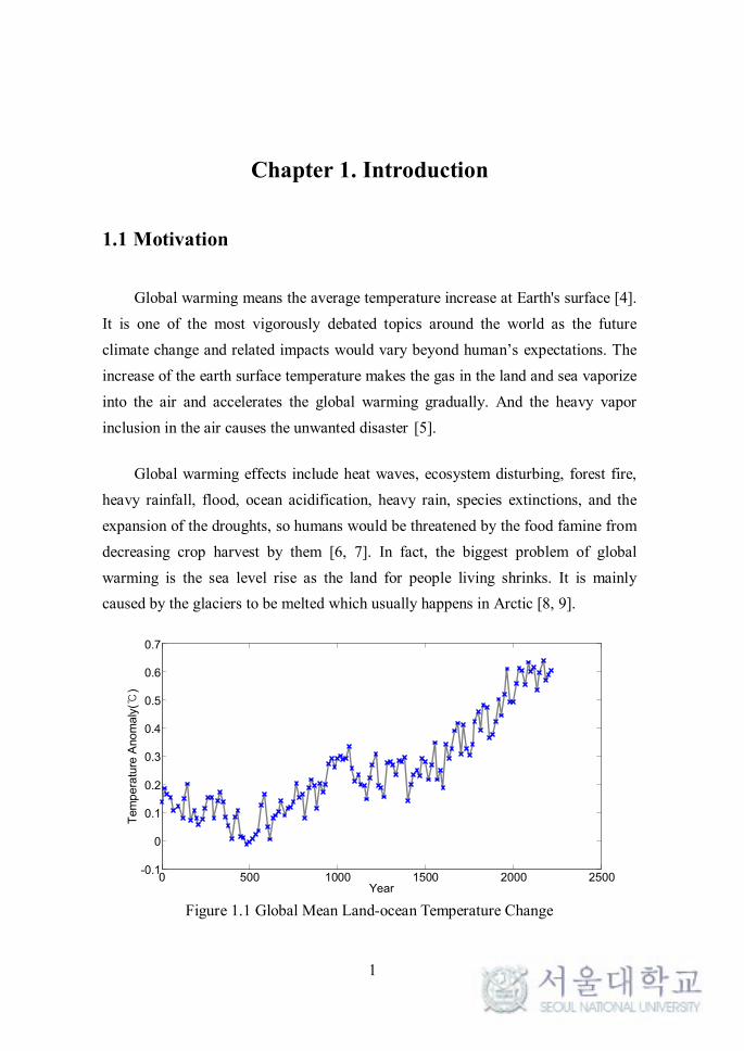
Global warming means the average temperature increase at Earth's surface [4].

It is one of the most vigorously debated topics around the world as the future

climate change and related impacts would vary beyond human’s expectations. The

increase of the earth surface temperature makes the gas in the land and sea vaporize

into the air and accelerates the global warming gradually. And the heavy vapor

inclusion in the air causes the unwanted disaster [5].

Global warming effects include heat waves, ecosystem disturbing, forest fire,

heavy rainfall, flood, ocean acidification, heavy rain, species extinctions, and the

expansion of the droughts, so humans would be threatened by the food famine from

decreasing crop harvest by them [6, 7]. In fact, the biggest problem of global

warming is the sea level rise as the land for people living shrinks. It is mainly

caused by the glaciers to be melted which usually happens in Arctic [8, 9].

Figure 1.1 Global Mean Land-ocean Temperature Change

0 500 1000 1500 2000 2500-0.1

0

0.1

0.2

0.3

0.4

0.5

0.6

0.7

Year

Tem

pe

ratu

re A

no

ma

ly(

)℃

2

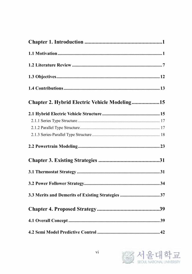
Figure 1.1 presents the global mean land-ocean temperature change. The

increase is mainly caused by the temperature increase in the oceans and the increase

tendency becomes heavier as it gets recent [10]. Therefore, finding the reason for

the global warming and setting up the solution is very urgent and important

assignment for the present generations.

Recently, IPPC (Intergovernmental Panel on Climate Change) announced that

the scientists were certain that the cause of the global warming is greenhouse gases

such as vapor, carbon dioxide, methane produced by human activities and was

recognized by the national science academies in 2010. Assuring these findings in

2013, IPCC stated that one of the largest inducer of the global warming is carbon

dioxide emissions from fossil fuel combustion [11]. The report in 2013 states:

“Human influence has been detected in warming of the atmosphere and the ocean,

in changes in the global water cycle, in reductions in snow and ice, in global mean sea

level rise, and in changes in some climate extremes. This evidence for human influence

has grown since AR4. It is extremely likely (95-100%) that human influence has been

the dominant cause of the observed warming since the mid-20th century.”

in IPCC report [12]. Therefore, the endeavors to overcome the disasters caused by

global warming are essentially required and the effort for an automobile industry

took the form of vehicle fuel economy improvement.

A fuel economy refers to the fuel efficiency relationship between the distance

traveled and the amount of fuel consumed by the vehicle. Fuel consumption can be

expressed in terms of volume of fuel to travel a distance, or the distance travelled

per unit volume of fuel consumed. Since the fuel consumption of vehicles is a

significant factor in the air pollution, and since importation of vehicle fuel can be a

large part of a nation's foreign trade, many countries impose some constraints for

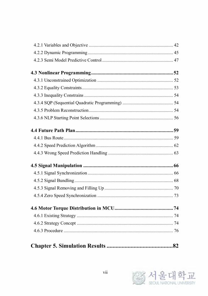
the fuel economy. As a result, the fuel economy in the automobile industry has

3

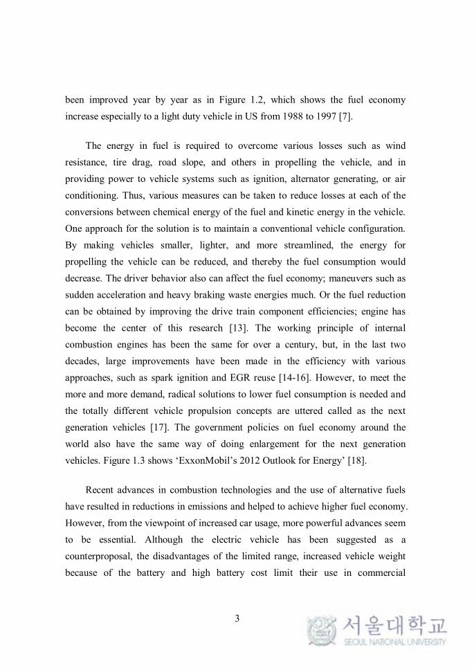
been improved year by year as in Figure 1.2, which shows the fuel economy

increase especially to a light duty vehicle in US from 1988 to 1997 [7].

The energy in fuel is required to overcome various losses such as wind

resistance, tire drag, road slope, and others in propelling the vehicle, and in

providing power to vehicle systems such as ignition, alternator generating, or air

conditioning. Thus, various measures can be taken to reduce losses at each of the

conversions between chemical energy of the fuel and kinetic energy in the vehicle.

One approach for the solution is to maintain a conventional vehicle configuration.

By making vehicles smaller, lighter, and more streamlined, the energy for

propelling the vehicle can be reduced, and thereby the fuel consumption would

decrease. The driver behavior also can affect the fuel economy; maneuvers such as

sudden acceleration and heavy braking waste energies much. Or the fuel reduction

can be obtained by improving the drive train component efficiencies; engine has

become the center of this research [13]. The working principle of internal

combustion engines has been the same for over a century, but, in the last two

decades, large improvements have been made in the efficiency with various

approaches, such as spark ignition and EGR reuse [14-16]. However, to meet the

more and more demand, radical solutions to lower fuel consumption is needed and

the totally different vehicle propulsion concepts are uttered called as the next

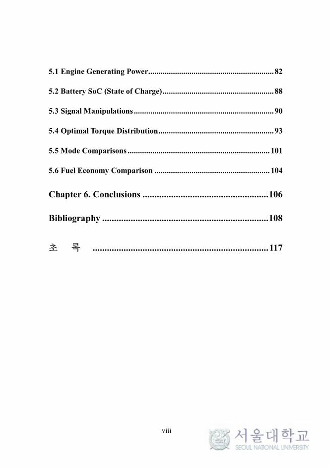
generation vehicles [17]. The government policies on fuel economy around the

world also have the same way of doing enlargement for the next generation

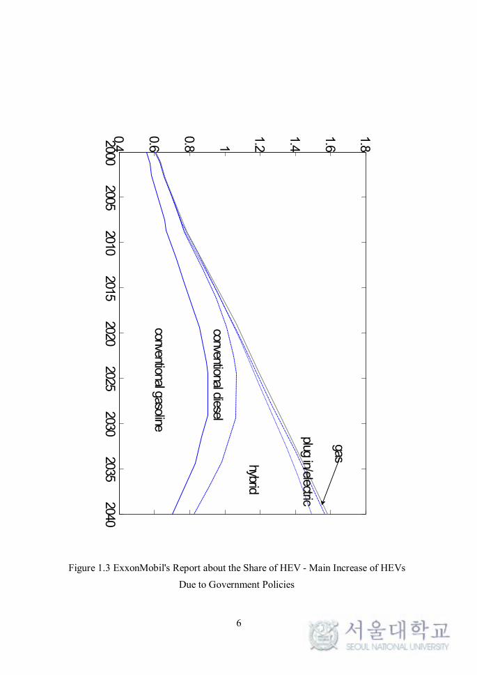
vehicles. Figure 1.3 shows ‘ExxonMobil’s 2012 Outlook for Energy’ [18].

Recent advances in combustion technologies and the use of alternative fuels

have resulted in reductions in emissions and helped to achieve higher fuel economy.

However, from the viewpoint of increased car usage, more powerful advances seem

to be essential. Although the electric vehicle has been suggested as a

counterproposal, the disadvantages of the limited range, increased vehicle weight

because of the battery and high battery cost limit their use in commercial

4

applications. Therefore, the hybrid electric vehicle which shows a short-term

approach improving fuel efficiency and reducing pollutant emissions of

automobiles has emerged as an alternative solution [19, 20].

There are many methodologies to achieve fuel economy increases or emission

reductions in hybrid vehicles. Among those methodologies, control strategy

research is one of the most important issues, as a hybrid vehicle strongly depends

on the supervisory control strategy, which influences each component of the

vehicle. Though the engine, generator, battery, motor and other components are

very powerful and effective, the resultant output performance without an

appropriate control strategy may be no more, or even less, than that of the internal

combustion engine [21].

5

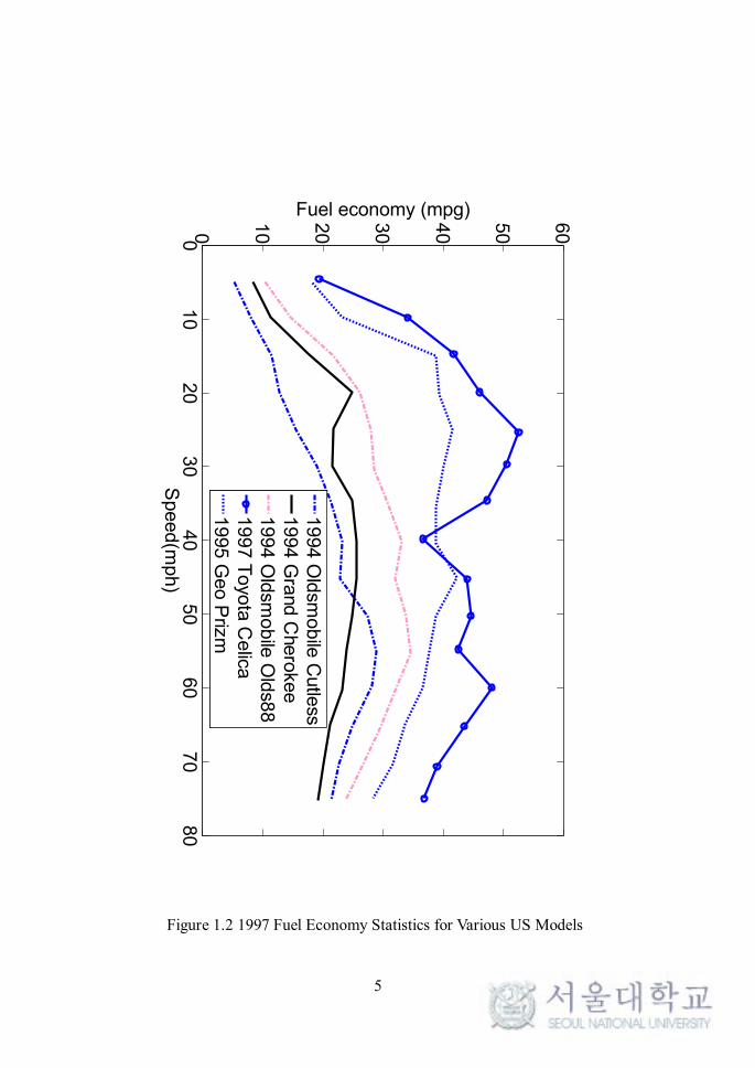
Figure 1.2 1997 Fuel Economy Statistics for Various US Models

010

20

30

40

50

60

70

80

0

10

20

30

40

50

60

Speed(m

ph)

Fuel economy (mpg)

1994 O

ldsm

obile

Cutle

ss1994 G

rand C

hero

kee

1994 O

ldsm

obile

Old

s88

1997 T

oyo

ta C

elica

1995 G

eo P

rizm

6

Figure 1.3 ExxonMobil's Report about the Share of HEV - Main Increase of HEVs

Due to Government Policies

20002005

20102015

20202025

20302035

20400.4

0.6

0.8 1

1.2

1.4

1.6

1.8

hybrid

gas

plug in/electric

conventional diesel

conventional gasoline

7

1.2 Literature Review

Basically, HEV reduces the fuel consumption by the following principles. First,

HEV recovers the vehicle’s kinetic energy by the regeneration of motors. The

regeneration of motor usually happens when the vehicle tries to stop and it works as

an electric generator. While braking the motor regenerative brakes, the motor

regenerative kinetic energy is convert into the electric energy, and is usually saved

in the battery. Thus, the traction motor with an inverter becomes an energy

converter while the mechanical brakes in ICE vehicles convert the kinetic energy

into the thermal energy, which cannot be used again [22]. Second, an HEV can shut

down the engine when it is needed. That is usually called ‘Idle Stop and Go’. As the

engine efficiency usually is bad when the load (torque) of the engine is little that

during idling and low load operations, using the motor only and turning off the

engine becomes much efficient that HEV can avoid the low efficiency operating

points of the engine. Third, the load leveling is possible with HEV. Since the

electric motor can provide a part of the torque, the best distribution of the load at

each time in the engine and motor unit is available and the motor can reduce the

burden of the engine. As a result, HEV can be designed with a smaller displacement

that ‘Downsizing of the engine’ can be achievable and the operating efficiency

improvements of the engine are realized [20, 23].

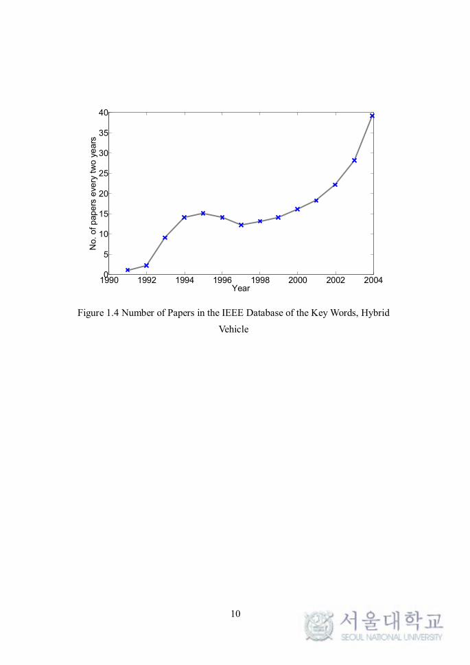
The fuel economy of HEV deeply depends on the vehicle; vehicle structure,

driving cycle, hybridization degree, component performance, component sizing,

and parameter tuning that the output performance of HEV ranges much according

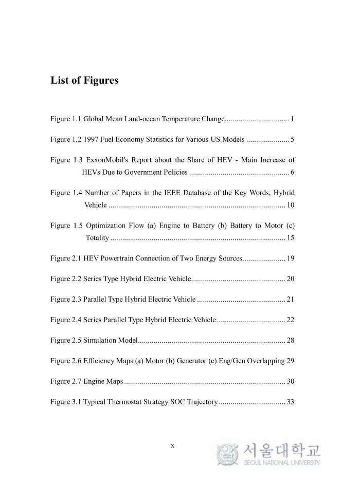
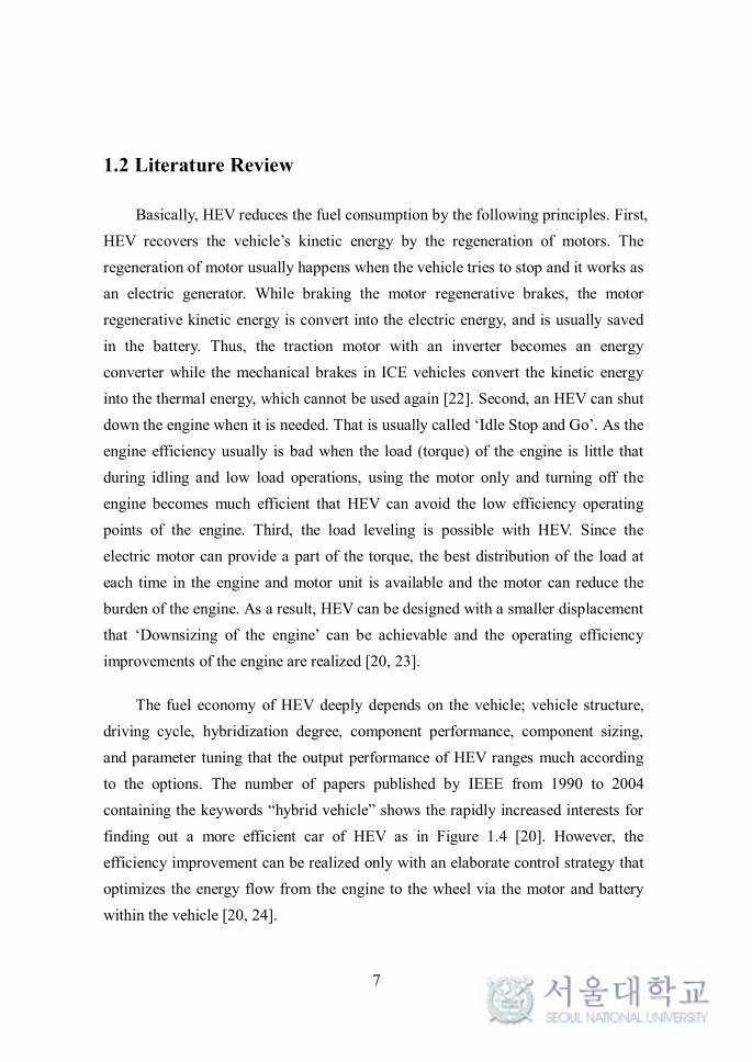
to the options. The number of papers published by IEEE from 1990 to 2004

containing the keywords “hybrid vehicle” shows the rapidly increased interests for

finding out a more efficient car of HEV as in Figure 1.4 [20]. However, the

efficiency improvement can be realized only with an elaborate control strategy that

optimizes the energy flow from the engine to the wheel via the motor and battery

within the vehicle [20, 24].

8

Among the HEV control strategies, two general trends are rule-based

strategies and optimization-based strategies. The rule based strategies are based on

heuristics, intuition, human expertise and even mathematical models without a

priori knowledge of a predefined driver cycle [25, 26]. Thermostat strategy, power

follower strategy and fuzzy rule-based strategy are the examples and their purpose

is load-leveling [27-30]. The limitation of heuristic control concepts is that the

various parameters depend strongly on the particular HEV system as well as on the

driving conditions. On the other hand, optimization-based strategies try to find a

global optimum using LP (Linear Programming), DP (Dynamic Programming), GA

(Genetic Algorithm), or etc. However, these strategies show the limit of non-

availability in the real-time environment [25, 26, 31, 32]. For example, DP is good

for the bench marks for the desirable references, however the strategy calculation

complexness and time deeply depend on the variable dimensions. If another energy

sources are included such as an ultra-capacitor, the calculation is almost impossible

as the calculation burden increases enormously. So, using SDP (Stochastic

Dynamic Programming), NDP (Neuro-Dynamic Programming), PMP (Pontryagin

Minimum Principal), or ECMS (Equivalent Consumption Minimization) was

suggested as a real-time solution [33-39]. However, even though the strategies

using the equivalent coefficient methodologies show the powerful performance,

handling the inequality constraint in the methodology and solving the problem

which cannot be analyzed analytically are so picky; or the equivalent coefficient

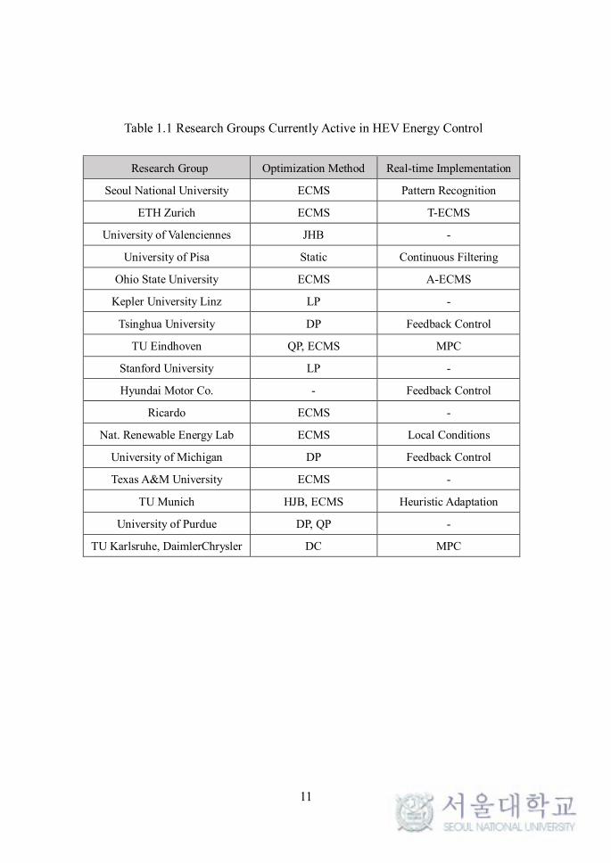
becomes so sensitive to the problem itself. Table 1 classifies publications in terms

of those optimal control techniques used around the world [20].

That is, these strategies still have some difficulties in their use, as it is not easy

to apply their mathematical backgrounds due to the complexity and size associated

with the controller required for the vehicle and still heavy calculation, which may

cause disability in the calculation or the harsh calculation time. Or, uncertainty

about future driving conditions is transferred to uncertainty on the optimal value of

the constant adjoint state approximation. So, in a real-time application, in spite of

9

fairly good, more complex, and sophisticated other strategies, the rule based

strategies, such as thermostat strategy or power follower strategy, have been still

realistic and powerful in series type hybrid electric vehicle [25, 40-43]. Or,

combinations of them are also considered for the better performance [1-3].

Nowadays, MPC (Model Predictive Control) which is applicable to real-time

model is introduced in the hybrid energy distribution. Usually, it requires an object

function of linear or nonlinear model and solver, where QP (Quadratic

Programming) or DP (Dynamic Programming) can be used. The hybrid model in

MPC can be applied for not only the linearized simple one but also the complex

nonlinear model. And, as of the real-time capability, both of the backward and the

forward hybrid vehicle models can be used. However, there are some demerits that

the initial points (using QP) dominates the result quality and the calculation burden

(using DP) is so heavy. Furthermore, as it requires the boundary conditions, the

speed information was surely required. Thus, in most cases, the speed was given

ideally and receding horizons for the every joint expectation was used, but it was

not true online energy distribution strategy [44, 45].

Therefore, if it is possible to overcome these weakness with more clear

standards of the energy distribution, better energy management strategy applicable

to the HEV system can be achievable: the real-time availability, calculation

exactness, and speedy calculation.

10

Figure 1.4 Number of Papers in the IEEE Database of the Key Words, Hybrid

Vehicle

1990 1992 1994 1996 1998 2000 2002 20040

5

10

15

20

25

30

35

40

Year

No.

of p

ap

ers

eve

ry t

wo

ye

ars

11

Table 1.1 Research Groups Currently Active in HEV Energy Control

Research Group Optimization Method Real-time Implementation

Seoul National University ECMS Pattern Recognition

ETH Zurich ECMS T-ECMS

University of Valenciennes JHB -

University of Pisa Static Continuous Filtering

Ohio State University ECMS A-ECMS

Kepler University Linz LP -

Tsinghua University DP Feedback Control

TU Eindhoven QP, ECMS MPC

Stanford University LP -

Hyundai Motor Co. - Feedback Control

Ricardo ECMS -

Nat. Renewable Energy Lab ECMS Local Conditions

University of Michigan DP Feedback Control

Texas A&M University ECMS -

TU Munich HJB, ECMS Heuristic Adaptation

University of Purdue DP, QP -

TU Karlsruhe, DaimlerChrysler DC MPC

12

1.3 Objectives

In this study, the optimal energy distribution strategy of series hybrid electric

bus was suggested. The strategy is unique, and especially suited for the series type

hybrid electric bus. The detailed objectives of this study are:

1. Developing the torque distribution strategy at the traction motor unit

2. Developing the energy distribution strategy from the engine to the battery

that the entire optimization of SHEV would be realized.

A number of strategies for power management of HEV were proposed in the

literature before to achieve optimality while keeping the realistic and practical

concept and this research shows a novel strategy for that. First, the control

technique which has semi-MPC structure is described from mathematical

viewpoints, which shows that the instantaneous optimal control with speedy

convergence that the battery and engine usages can be close to an optimal solution

of DP. In the strategy, NLP is used for the objective function optimization. And the

speed prediction of future path plan was used for the load and boundary condition

decision with a real bus data. Furthermore, additional techniques such as signal

removing, flattening, fill up, and synchronizing with zero vehicle speed was also

used for the performance improvement. Second, the traction motor unit torque

distribution which is uniquely needed for the dual traction motors were considered

for the fuel economy improvement. The performance of the hybrid vehicle using

the proposed control algorithm is evaluated by comparison the proposed strategy to

global optimal control algorithm based on DP and other baseline rule based

strategies such as thermostat strategy and power follower strategy.

13

1.4 Contributions

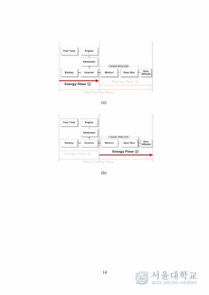
The contribution of this research is, first, the full optimization of SHEV was

achieved from the engine to the motor as in Figure 1.5(c). In the previous SHEV

optimal energy distribution researches, the energy flow optimization was achieved

just in ‘Energy Flow ①’ such that even though there is another chance which can

be added to improve the performance of SHEV, the optimization was just a half.

Because the performance achieved in other competitive hybrid types were with the

total powertrain components that the performance comparison with the half

optimization SHEV was unfair. So, this research shows the best availability of

series type hybrid electric vehicle, especially for dual traction motor mount. The

second contribution of this research is the proposed strategy is uniquely applicable

powerful strategy for the series type hybrid electric intra-buses. This character

comes from the independent operation between engine/generator unit and motor

unit. Thus, the signal manipulation and torque distribution also become possible.

The third contribution is this research gives the far precise answer of ‘How much to

generate?’ and “When to generate?” at once which were recognized as the

weaknesses of the existing rule based strategies. And final contribution is this

strategy uses NLP for the realistic forward model first and find a global sub-

optimum.

To conclude, this strategy suggest a fuel usage reduction methodology for the

intra-city bus. It is very worthy as its character is unique, clear, efficient, and

practical that solves the nonlinear SHEV energy management problem.

14

(a)

(b)

15

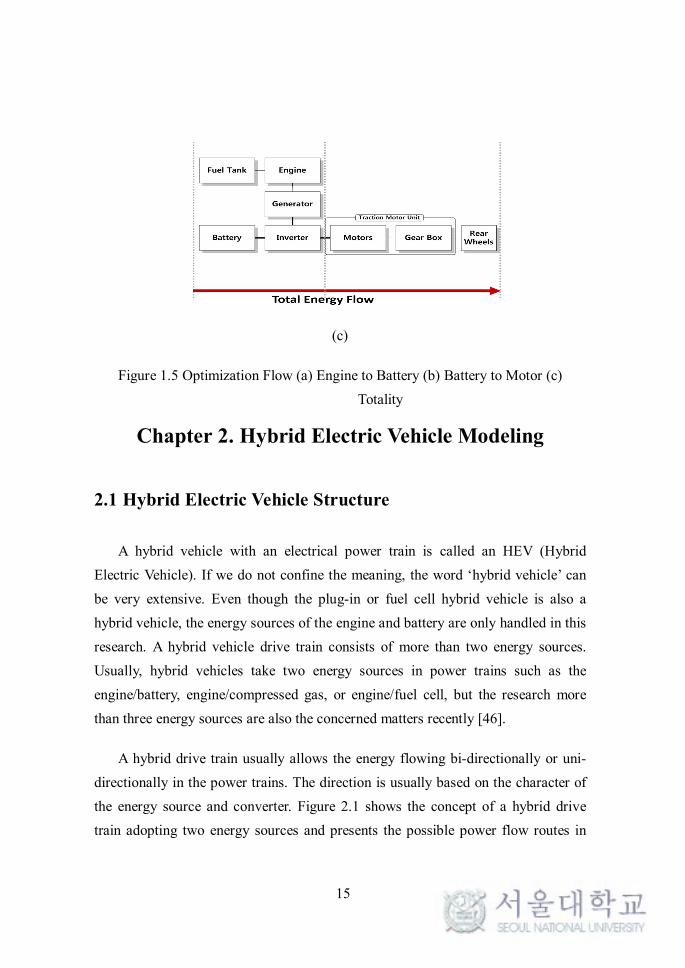
(c)

Figure 1.5 Optimization Flow (a) Engine to Battery (b) Battery to Motor (c)

Totality

Chapter 2. Hybrid Electric Vehicle Modeling

2.1 Hybrid Electric Vehicle Structure

A hybrid vehicle with an electrical power train is called an HEV (Hybrid

Electric Vehicle). If we do not confine the meaning, the word ‘hybrid vehicle’ can

be very extensive. Even though the plug-in or fuel cell hybrid vehicle is also a

hybrid vehicle, the energy sources of the engine and battery are only handled in this

research. A hybrid vehicle drive train consists of more than two energy sources.

Usually, hybrid vehicles take two energy sources in power trains such as the

engine/battery, engine/compressed gas, or engine/fuel cell, but the research more

than three energy sources are also the concerned matters recently [46].

A hybrid drive train usually allows the energy flowing bi-directionally or uni-

directionally in the power trains. The direction is usually based on the character of

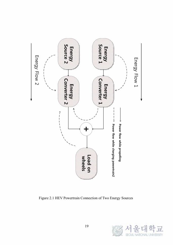
the energy source and converter. Figure 2.1 shows the concept of a hybrid drive

train adopting two energy sources and presents the possible power flow routes in

16

the power train [22]. The drive train can choose the energy flow in the vehicle by

command signal made by HCU (Hybrid Control Unit) and the common pattern in

energy flow are as follows;

First, power train 1 alone delivers its power to the load. Usually this might be

the engine and shoulders all road load burden which starts from the tire. Second,

power train 2 delivers its power to the load alone. If we imagine power train 2 to be

the motor/battery, it also can burden the road load from the tire. And the answer to

the question ‘How much to share the burden?’ is the third one. The power train 1

and 2 deliver their power to the load simultaneously. This is usually made

according to the efficiency leveling of the system that all the energy flow share

ratio is made differently to achieve the best fuel economy of the system. Fourth,

power train 2 obtains energy from the load by regenerative braking when the

vehicle decelerate. Fifth, power train 2 obtains power from power train 1 when the

battery (energy converter2) is deficient. This means the battery is deficient in SoC

(State of Charge). The energy flow 6 is the power flow from power train 1 to power

train 2 and the load simultaneously, and the power flow 7 is from power train 2 to

power train 1 and the load simultaneously, vice versa. Those two cases makes the

power more than load and the surplus power can be provided to the other part.

Eighth, power train 1 can delivers its power to power train 2, and power train 2

delivers its power to the load. Finally, power train 1 delivers its power to the load,

and the load delivers the power to power train 2 [22]. These two are somewhat

unusual cases as the energy saving to the other part would experience the losses at

each component again when it propelling the vehicle and shares the load in the

future. Therefore, the freedom of the energy flow route is very extensive in the

hybrid power train [22].

HEVs are basically classified into three kinds, series hybrid, parallel hybrid,

series-parallel hybrid, which are shown in Figure 2.2 to 2.4, but the classifications

are not clear as there are lots of the derivation of hybrid types and it may cause

some confusions (sometimes series-parallel type is divided to two categories). But

17

the clear one is there are two kinds of energy flows in the drive train, mechanical

and electrical power flows [22].

Among those hybrid types, SHEV (Series Hybrid Electric Vehicle) was chosen

as a research target in this research as the outstanding performance of SHEV intra-

city bus was proven in other researches but has still has some possibility of

performance improvements [47, 48]. However, the structures of other types are also

introduced in this Chapter for a better understanding. Each configuration would be

introduced with simple schematics, and the characteristic of each configuration will

be discussed briefly [49].

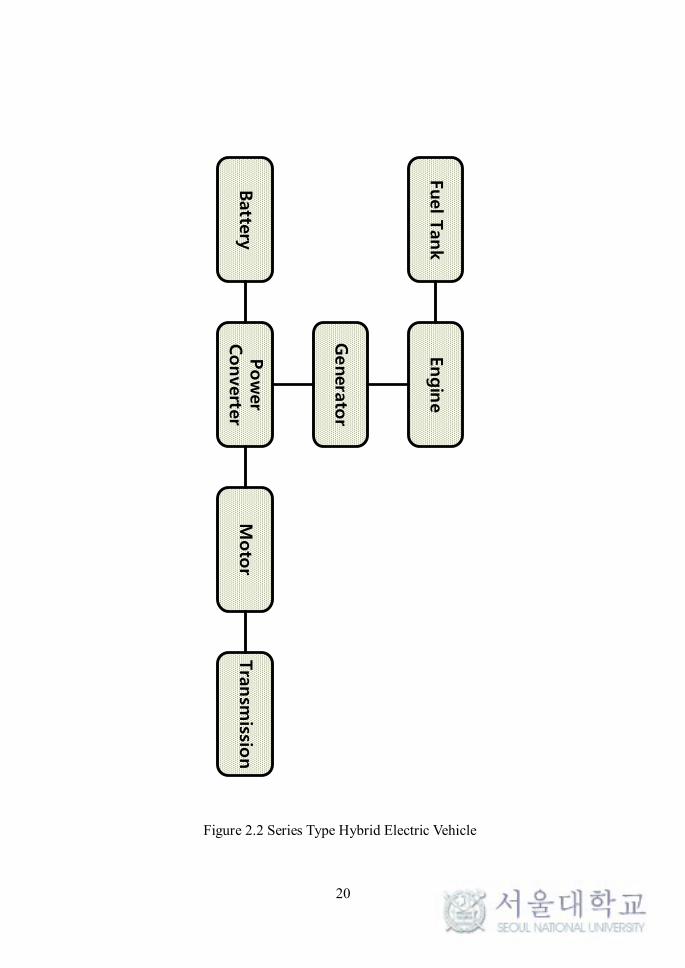
2.1.1 Series Type Structure

This type hybrid vehicle has two different electrical power trains. The first one

is the generator coupled with the engine and used for the power generation to the

battery, of single power direction. And the other is traction motor used for the

vehicle traction. The simultaneous vehicle traction is not considered in this

structure and the regeneration of the energy is very large as the capacity of the

traction motor is the biggest among the hybrid types. So, it is similar to the electric

vehicle. The engine, and the generator constitute the primary energy sources that

the battery functions as an energy bumper. The configuration of the series hybrid

system is unique as the engine operation is independently connected to the

operation of the traction motor, so electric motor produces all propulsion force

without any interferences of the engine/generator unit. Thus, optimal operation

engine is very easy compared to the other type hybrid vehicle. But, each component

capacity becomes very large and, as the energy conversion might happens in the

power train often, managing the energy flow is very important [22, 34, 43].

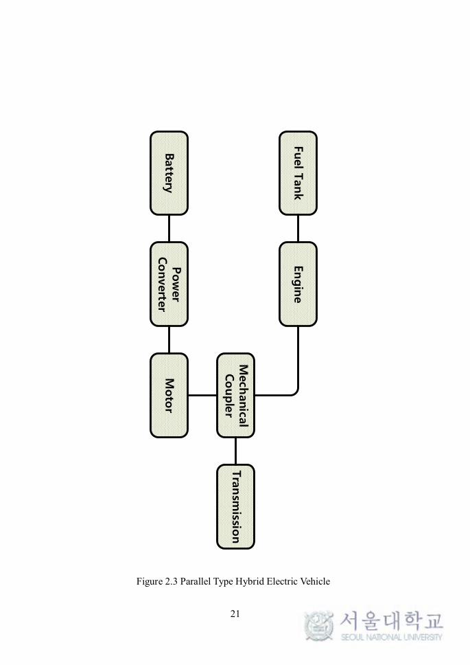
2.1.2 Parallel Type Structure

18

The main character causing all features is the engine and motor coupling by the

mechanical coupler. The engine is the primary energy source for the traction, and

the battery and electric motor are the bumper and auxiliary energy source. The big

difference compared to the series type hybrid structure is the traction torque can be

provided simultaneously by the engine and motor, as the engine, the electric motor

and the gear box are coupled by automatically controlled clutches. The motor size

is much smaller than that of series type hybrid vehicle and the speed ratio between

the motor and engine holds constant that how to distribute the torque is main

concern of this type hybrid vehicle. The development of this type vehicle is made

based on existing ICE vehicle that potential of the improvement might not be

significant. The first mass production parallel hybrid sold outside Japan was Honda

Insight and many productions in Hyundai motors nowadays adopt this type hybrid

vehicle [22, 35].

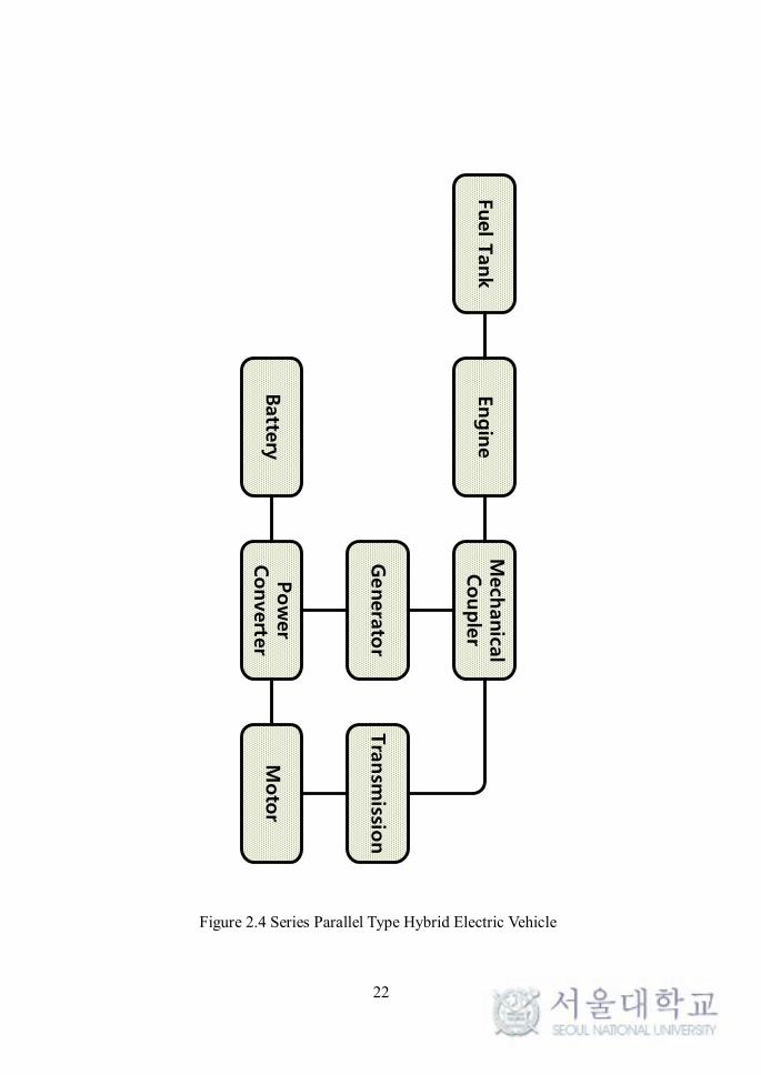
2.1.3 Series-Parallel Type Structure

The series-parallel hybrid system is usually called power-split type and uses an

electric motor to drive at low loads and speeds while uses the engine to at middle or

high loads/speeds. They work together or individually depending on the required

power from the road load. Each component operate most effectively and usual

hybrid drive trains in series-parallel hybrid type adopts a planetary gear to achieve

it. The engine gives its power to the sun gear by transmission, which modifies the

required speed–torque profile of the engine. And the electric motor supplies its

power to the ring gear. The Toyota Hybrid System is very famous for this type

hybrid vehicle and the control of this type system is very complex and sophisticated

[22, 31].

19

Energ

y

Source

1Energ

y

Converte

r 1

Energ

y

Source

2Energ

y

Converte

r 2

+ Pow

er flo

w w

hile

pro

pellin

g

Pow

er flo

w w

hile

charg

ing p

ow

ertra

in2

Load o

n

wheels

Energ

y F

low

1

Energ

y F

low

2

Figure 2.1 HEV Powertrain Connection of Two Energy Sources

20

Fuel T

ank

Engin

e

Genera

tor

Pow

er

Converte

rBatte

ryM

oto

rTra

nsm

ission

Figure 2.2 Series Type Hybrid Electric Vehicle

21

Fuel T

ank

Engin

e

Tra

nsm

ission

Pow

er

Converte

rBatte

ryM

oto

r

Mechanic

al

Couple

r

Figure 2.3 Parallel Type Hybrid Electric Vehicle

22

Fuel T

ank

Engin

e

Tra

nsm

ission

Pow

er

Converte

rBatte

ryM

oto

r

Mech

anica

l Couple

r

Genera

tor

Figure 2.4 Series Parallel Type Hybrid Electric Vehicle

23

2.2 Powertrain Modeling

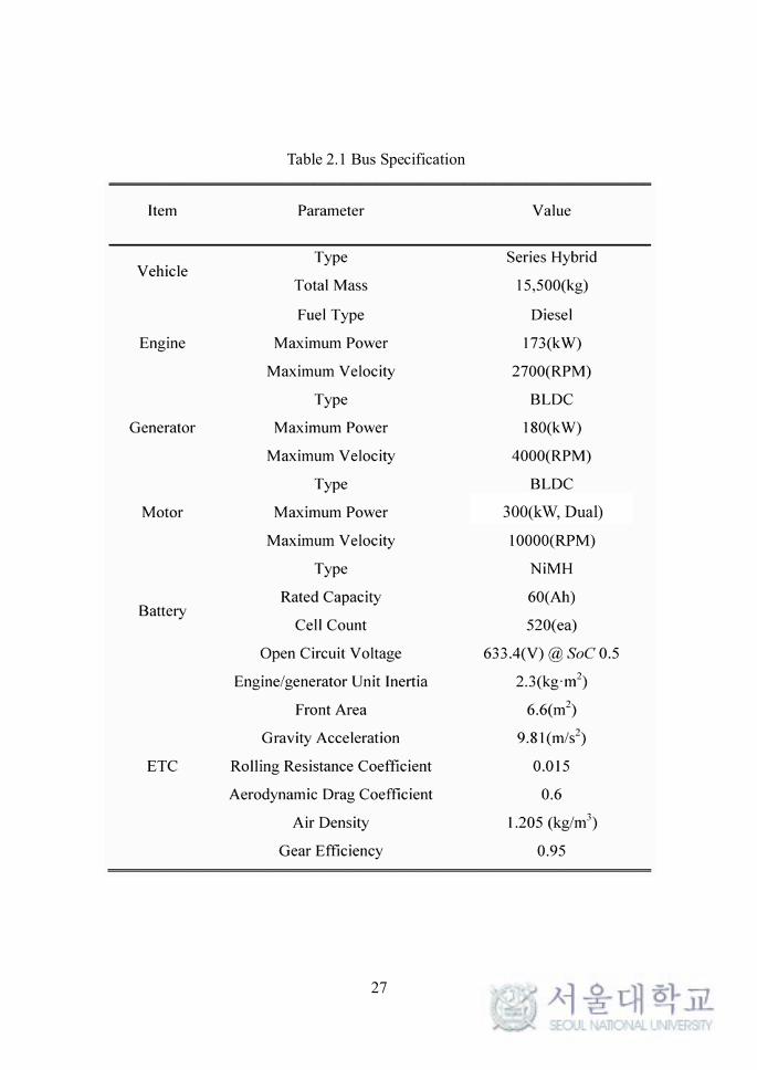
Table 2.1 shows the specifications for a series type hybrid bus. The bus is an

intra-city bus for the Seoul city transit system and uses dual motors as a traction

motor. The powers of the engine, generator and motor are 173 kW, 180 kW and 300

kW (Dual), respectively. The slop of the road, the wind velocity and the moment of

inertia for the traction motor was ignored, as the rotational inertia of the motor is

negligible in comparison to the inertia of the vehicle [50].

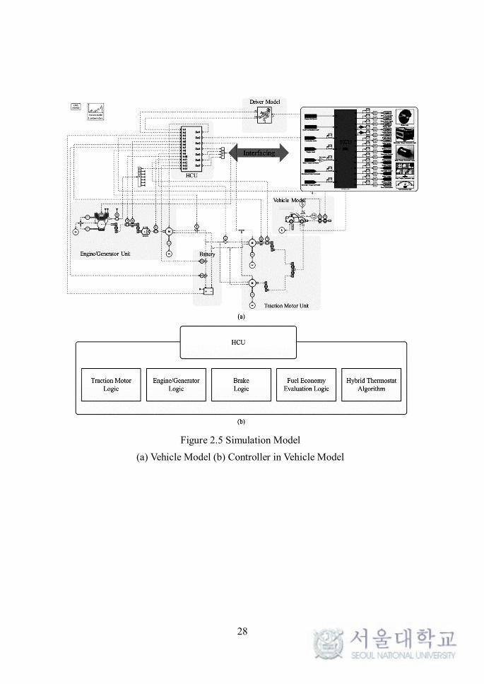
In this research, the hybrid electric bus was developed with a forward

simulation model. The bus model was developed in AMESim which considers the

inertia of the system with control logic in Simulink. Figure 2.5 shows the

simulation model for this research. It consists of the engine/generator unit, the

battery, the vehicle model, the driver model, HCU (Hybrid Control Unit), the gears

between the components, and dual traction motors where inverter effect is included

in the motor efficiency map. Basically, the battery model receives electrical energy

from the engine/generator unit and transfers it to the dual traction motors. And dual

traction motor torque is enlarged with reduction gears, so the summation gear

gathers both torques at once and transfers it to the wheels. In the end, the traction

motor torque is transferred to the vehicle model where the road load is calculated

and the acceleration overcoming it is made with the control of the driver model.

HCU interfaces with Simulink and includes the traction motor logic, the

engine/generator torque logic, the brake logic, the fuel economy evaluation, and the

hybrid control algorithm.

The basic equations in the modeling are defined below [47, 48, 51-58]. The

output engine power eP is expressed by:

( , )

e e e e

e e e f

P Load w

w P

t

h t

= ´ ´

= ´ (2.1)

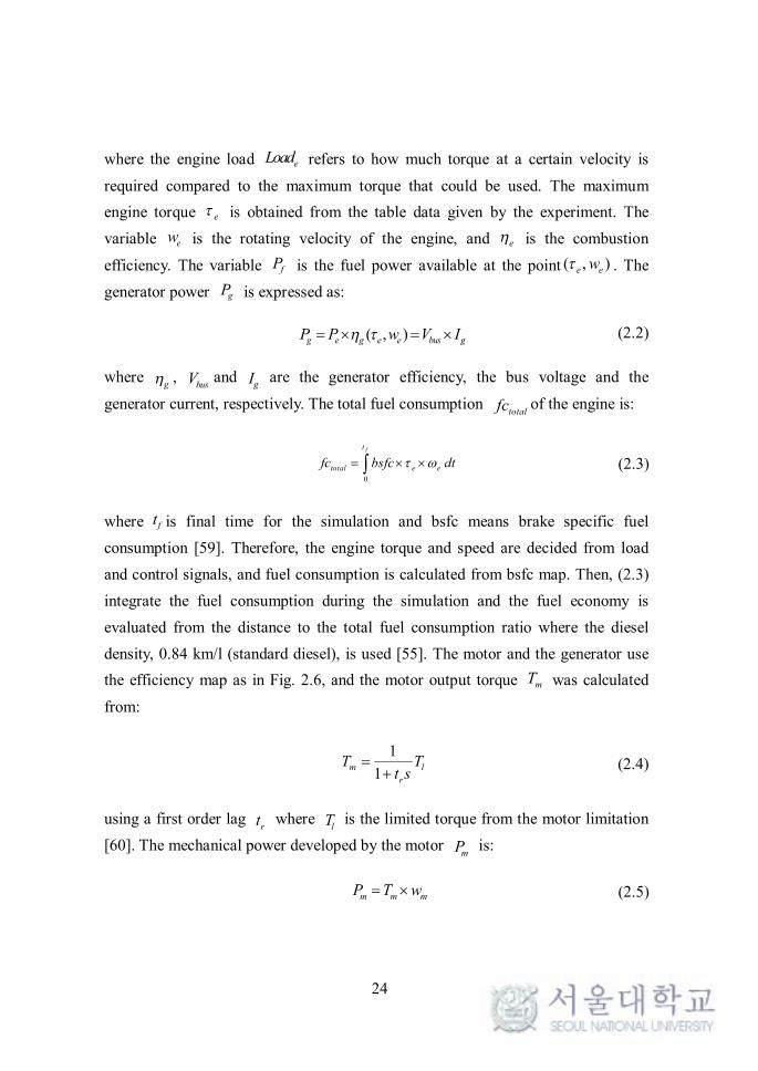
24

where the engine load eLoad refers to how much torque at a certain velocity is

required compared to the maximum torque that could be used. The maximum

engine torque et is obtained from the table data given by the experiment. The

variable ew is the rotating velocity of the engine, and eh is the combustion

efficiency. The variable fP is the fuel power available at the point ( , )e ewt . The

generator power gP is expressed as:

( , )g e g e e bus gP P w V Ih t= ´ = ´ (2.2)

where gh ,

busV and gI are the generator efficiency, the bus voltage and the

generator current, respectively. The total fuel consumption totalfc of the engine is:

0

ft

total e efc bsfc dtt w= ´ ´ò (2.3)

where ft is final time for the simulation and bsfc means brake specific fuel

consumption [59]. Therefore, the engine torque and speed are decided from load

and control signals, and fuel consumption is calculated from bsfc map. Then, (2.3)

integrate the fuel consumption during the simulation and the fuel economy is

evaluated from the distance to the total fuel consumption ratio where the diesel

density, 0.84 km/l (standard diesel), is used [55]. The motor and the generator use

the efficiency map as in Fig. 2.6, and the motor output torque mT was calculated

from:

1

1m l

r

T Tt s

=+

(2.4)

using a first order lag rt where

lT is the limited torque from the motor limitation

[60]. The mechanical power developed by the motor mP is:

m m mP T w= ´ (2.5)

25

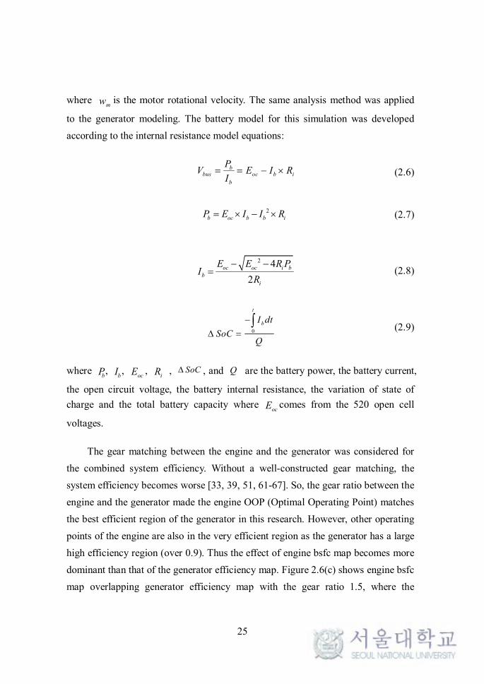
where mw is the motor rotational velocity. The same analysis method was applied

to the generator modeling. The battery model for this simulation was developed

according to the internal resistance model equations:

bbus oc b i

b

PV E I R

I= = - ´ (2.6)

2b oc b b iP E I I R= ´ - ´ (2.7)

2 4

2

oc oc i bb

i

E E R PI

R

- -= (2.8)

0

t

bI dt

SoCQ

-

D =ò (2.9)

where bP,

bI , ocE ,

iR , SoCD , and Q are the battery power, the battery current,

the open circuit voltage, the battery internal resistance, the variation of state of

charge and the total battery capacity where ocE comes from the 520 open cell

voltages.

The gear matching between the engine and the generator was considered for

the combined system efficiency. Without a well-constructed gear matching, the

system efficiency becomes worse [33, 39, 51, 61-67]. So, the gear ratio between the

engine and the generator made the engine OOP (Optimal Operating Point) matches

the best efficient region of the generator in this research. However, other operating

points of the engine are also in the very efficient region as the generator has a large

high efficiency region (over 0.9). Thus the effect of engine bsfc map becomes more

dominant than that of the generator efficiency map. Figure 2.6(c) shows engine bsfc

map overlapping generator efficiency map with the gear ratio 1.5, where the

26

numbers between the lines show engine bsfc and the numbers between the dot-lines

show the generator efficiency. The circle points are sample power follower

operating points and the cross points are sample hybrid thermostat operating points

which would be explained in the next Chapter. As mentioned above, almost all

points are in the high efficiency region of the generator, so the efficiency of the

system is directly influenced by the engine efficiency, bsfc map.

27

Table 2.1 Bus Specification

300(kW, Dual)

28

Figure 2.5 Simulation Model

(a) Vehicle Model (b) Controller in Vehicle Model

29

(a)

(b)

Maximum Generator Torque

Maximum Engine Torque

260

208

312

364

0.93

0.9

0.9 0.83

― number ― : Generator Efficiency --- number --- : Engine bsfc

(c)

Figure 2.6 Efficiency Maps (a) Motor (b) Generator (c) Eng/Gen Overlapping

Speed(rpm)

Torq

ue(N

m)

0 1000 2000 3000 4000

100

200

300

400

500

600

700

800

900

0.78

0.8

0.82

0.84

0.86

0.88

0.9

0 500 1,000 1,500 2,000 2,500 3,000 3,500 4000

100

200

300

400

500

600

Generator Velocity(RPM)

Gen

erat

or

Torq

ue(N

·m)

0.6

0.65

0.7

0.75

0.8

0.85

0.9

30

Figure 2.7 Engine Maps

(a) Bsfc Map (b) OOL (Optimal Operating Line)

31

Chapter 3. Existing Strategies

This Chapter shows the conventional strategies which were often used to

evaluate series type hybrid electric vehicle system fuel economy. As of the simple

structure, even though lots of other strategies were suggested at the case of parallel

hybrid or parallel-series hybrid, in the case of series type hybrid vehicle, theses rule

based strategies are often used as a baseline strategies. Furthermore, the recent

studies still upbuild these strategies for a better performance.

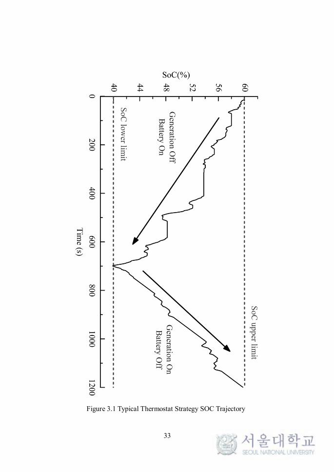
3.1 Thermostat Strategy

Thermostat strategy is a rule based on/off strategy that considers the SoC (state

of charge) limitation of the battery. Fig. 3.1 shows the typical trend observed when

using this strategy. The strategy turns on the engine/generator unit when the battery

SoC approaches the lower limit, and turns off the engine when the battery SoC

approaches the upper limit, where the upper and lower boundaries are selected

based on the internal resistance of the battery. Because this strategy uses an

engine/generator unit at the OOP, the operating efficiency of the engine is very high

[34, 47, 68].

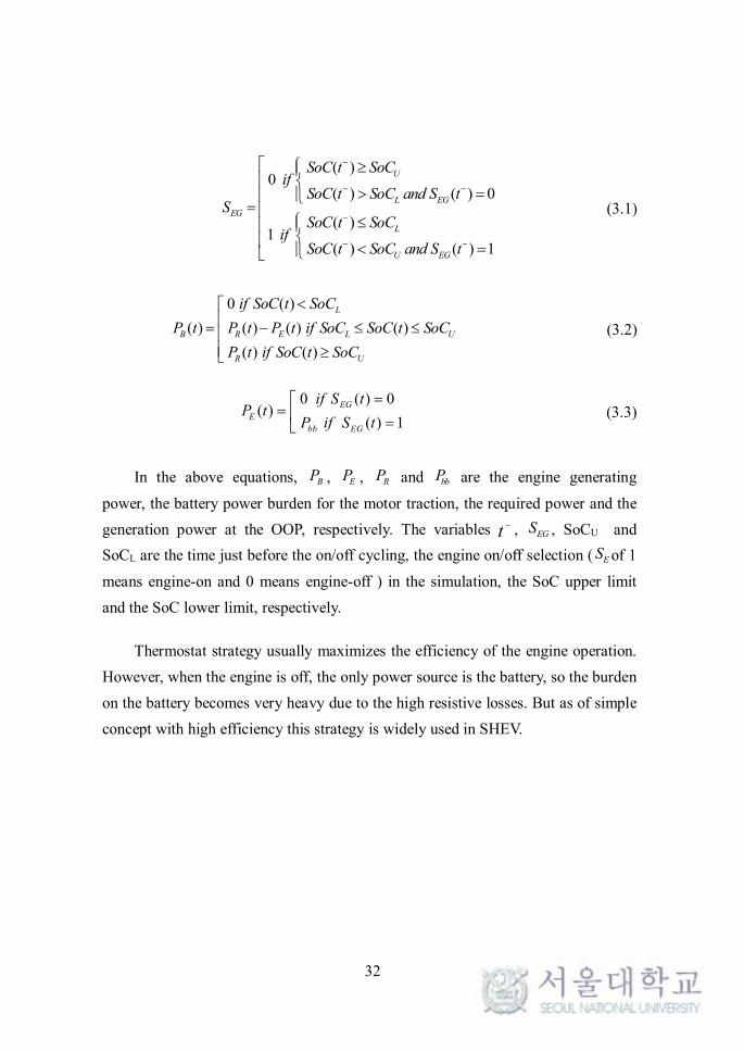
Equation (3.1) shows the turn on/off criteria for the thermostat strategy. The

engine/generator unit power command is computed in (3.2) and (3.3) [25, 26, 64,

69, 70]:

32

( )0

( ) ( ) 0

( )1

( ) ( ) 1

U

L EG

EG

L

U EG

SoC t SoCif

SoC t SoC and S tS

SoC t SoCif

SoC t SoC and S t

-

- -

-

- -

é ì ³ïê í

> =ïê î= ê

ì £ïêíê < =ïîë

(3.1)

0 ( )

( ) ( ) ( ) ( )

( ) ( )

L

B R E L U

R U

if SoC t SoC

P t P t P t if SoC SoC t SoC

P t if SoC t SoC

<éê

= - £ £êê ³ë

(3.2)

0 ( ) 0( )

( ) 1

EG

E

bb EG

if S tP t

P if S t

=é= ê =ë

(3.3)

In the above equations, BP , EP , RP and bbP are the engine generating

power, the battery power burden for the motor traction, the required power and the

generation power at the OOP, respectively. The variables t- , EGS , SoCU and

SoCL are the time just before the on/off cycling, the engine on/off selection ( ES of 1

means engine-on and 0 means engine-off ) in the simulation, the SoC upper limit

and the SoC lower limit, respectively.

Thermostat strategy usually maximizes the efficiency of the engine operation.

However, when the engine is off, the only power source is the battery, so the burden

on the battery becomes very heavy due to the high resistive losses. But as of simple

concept with high efficiency this strategy is widely used in SHEV.

33

Figure 3.1 Typical Thermostat Strategy SOC Trajectory

34

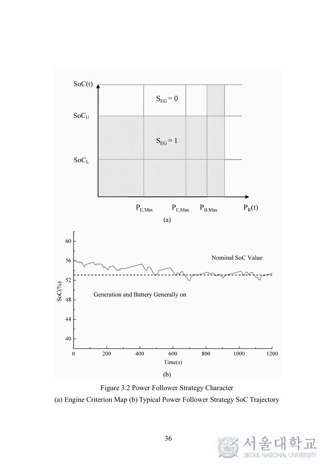
3.2 Power Follower Strategy

Power follower strategy appoints the engine/generator unit as the main power

source, and the controller adjusts the output power to follow the power requirement

of the vehicle. The control logic of power follower strategy is based on the map in

Figure 3.2(a) with the corresponding power output determined by (3.4) to (3.6).

EP a , ,E MinP , ,E MaxP and ,B MaxP are the base of the engine power, which considers the

battery SoC (a is the design variable for the control optimization); the minimum

available engine power; the maximum available engine power; and the maximum

available battery supply power, respectively. In Figure 3.2(a), there are four

operation modes for the engine/generator set by EP . If the current SoC is greater

than the target SoC, the power generated is smaller than the required power and the

battery is discharged. When the current SoC is lower than the target SoC, more

power is generated than required and the battery can recharge. The gray area in Fig.

3.2(a) prevents frequent on/off cycling of the engine and the engine operates around

the OOL (Optimal Operating Line) [34-36]:

, ,

, ,

, ,

0 ( ) 0

( ) 1 ( )( )

( ) ( ) 1 ( )

( ) 1 ( )

EG

E Min EG E E Min

E

E EG E Min E E Max

E Max EG E E Max

if S t

P if S t and P t PP t

P t if S t and P P t P

P if S t and P t P

a

a a

a

=éê = <ê=ê = £ <ê

= ³êë

(3.4)

( ) [ ( )]2

U LE R

SoC SoCP t P SoC ta a

+= + ´ - (3.5)

( ) ( ) ( ) 1( )

( ) ( ) 0

R E EG

B

R EG

P t P t if S tP t

P t if S t

- =é= ê =ë

(3.6)

35

Power follower strategy SoC tendency, for example, is shown in Figure 3.2(b).

The SoC change is not as much as that of the thermostat strategy, but the

engine/generator unit is active under almost all driving conditions, except for those

when a very low driving power is required and the SoC is greater than SoCU. This

algorithm is important in that the battery efficiency can be increased as the engine

shares the burden of the battery. Thus, a reduction in the current flow from the

battery can be achieved, and the resistive losses due to the large current can be

avoided. The optimization of this strategy can be carried out according to the

variance of a as in (3.5).

36

Figure 3.2 Power Follower Strategy Character

(a) Engine Criterion Map (b) Typical Power Follower Strategy SoC Trajectory

37

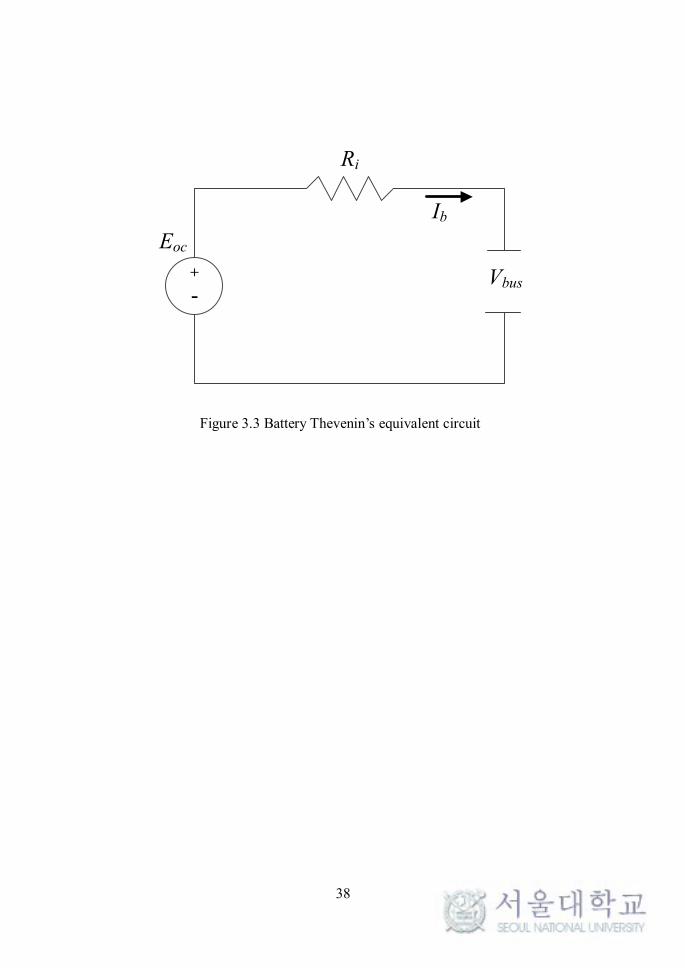
3.3 Merits and Demerits of Existing Strategies

Thermostat strategy generally uses a single optimal operating point as a

command signal. Therefore, when the controller turns on the engine, the engine

operating point soon arrives at the OOP. Running at this operating point allows for

high system efficiency. However, some disadvantages occur when the discharge

starts and the battery is only in use for the traction motor. If the required power is

low, the current from the battery in Figure 3.3 is small, and the battery internal

resistance loss is negligible. However, when high power is required, a large current

will flow from the battery to the traction motors, and the internal resistive losses in

the battery increase enormously. As the variation effect of Ib is more dominant than

that of internal resistance Ri or the open circuit voltage Eoc , a large value for Ib

when using the thermostat strategy makes the system efficiency very poor [12].

Furthermore, the hard use of the battery makes the battery life becomes less and

less.

On the other hand, the disadvantage of power follower strategy is that this

strategy usually uses less efficient operating point than the OOP as an engine

command operating signal. Even though the power follower strategy works using

OOL in Figure 2.7(b), OOL itself shows deep bsfc variation according to the power

generated by the engine. Thus, the engine operating point efficiencies usually much

less than OOP might be used. That is because the generation power of the power

follower strategy is constrained by SoC condition in (3.5) that the command signal

might goes to less efficient operating point inadvertently. Furthermore the operating

point commands require transient time to make the engine operating points arriving

at the designated commands but as the command changes so rapidly, the engine

operating points swing in the bsfc map before arriving at the target operating points

with less efficiency.These are the limitations of the rule based strategies, as the rule

are usually made by heuristic perceptions.

38

+

-

Eoc

Ri

Vbus

Ib

Figure 3.3 Battery Thevenin’s equivalent circuit

39

Chapter 4. Proposed Strategy

4.1 Overall Concept

This chapter presents the energy management strategy that is derived from the

optimal control theory. First, a formal problem definition is given, by expressing

the total fuel consumption minimization along the driving cycle as a function of the

control variables. Then, semi MPC (Model Predictive Control) is used to explicitly

use the dynamic model to predict the system evolution in the future where the

optimal control sequence, NLP (Nonlinear Programming), has been applied to

minimize the object function, under the assumption that the next section of the

driving cycle is predictable in advance. Then, the speed prediction algorithm by the

least square method was carried out, as NLP requires the boundary condition and

road load for the next Chapter in advance. As a result, the method could calculate

the engine operating set-points of the next section in the model from the engine to

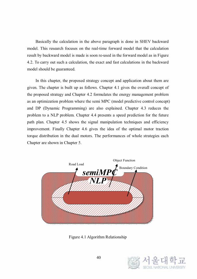
the battery very efficiently. Figure 4.1 shows the relation concept of this algorithm.

DP gives a very good reference as it is well known for the global optimal

solution. However, even though the calculation performance is guaranteed, the

computation time for the real-time implementation is so important, whereas the

computation time of DP is too long. Therefore, DP can be only the performance

comparison reference. In this research, to achieve further calculation efficiency

improvements, the additional real-time strategy techniques such as signal

synchronizing, signal bundling, signal removing, signal filling up, and zero speed

synchronizing are also suggested, which are uniquely adoptable for SHEV.

Finally, MTU (Motor Traction Unit) torque distribution was proposed which is

unique to dual traction motors and not considered in other researches. As the

efficiency increase by those methods are achieved without changing the structure or

alternating the component of SHEV, the value of this research increases.

40

Basically the calculation in the above paragraph is done in SHEV backward

model. This research focuses on the real-time forward model that the calculation

result by backward model is made is soon re-used in the forward model as in Figure

4.2. To carry out such a calculation, the exact and fast calculations in the backward

model should be guaranteed.

In this chapter, the proposed strategy concept and application about them are

given. The chapter is built up as follows. Chapter 4.1 gives the overall concept of

the proposed strategy and Chapter 4.2 formulates the energy management problem

as an optimization problem where the semi MPC (model predictive control concept)

and DP (Dynamic Programming) are also explained. Chapter 4.3 reduces the

problem to a NLP problem. Chapter 4.4 presents a speed prediction for the future

path plan. Chapter 4.5 shows the signal manipulation techniques and efficiency

improvement. Finally Chapter 4.6 gives the idea of the optimal motor traction

torque distribution in the dual motors. The performances of whole strategies each

Chapter are shown in Chapter 5.

Speed Prediction

NLPsemiMPC

Object Function

Boundary ConditionRoad Load

Figure 4.1 Algorithm Relationship

41

Figure 4.2 Backward Model to Forward Model Transplant

42

4.2 Semi Model Predictive Control

The basic idea of controlling the engine power is initiated by finding the most

efficient operating points which would result in achieving the best fuel economy in

the vehicle. It can be possible by considering the correlation of each component. In

this Chapter, the energy flow from engine/generator unit to the battery is usually

handled when the road load from the traction motor is given.

4.2.1 Variables and Objective

The problem is for the backward model and this control problem can be

formulated as a discrete state space problem. Using discrete time, the system

dynamics can be described as follows [13, 71]:

( 1) ( ( ), ( ), )x k f x k u k k+ = (4.1)

and the object function is:

0

( ( ), ( ), )n

k

J x k u k k t=

Då (4.2)

where the constraints are:

( ( ), ( ), ) 0x k u k kx = (4.3)

( ( ), ( ), ) 0x k u k kz £ (4.4)

Usually, x(k) are the state variables, such as vehicle speed, engine speed, and

energy storage levels and u(k) are the control variables like the engine generating

power and x is equality constraints with z of inequality constraints. In this

application, the relevant state is the energy level in the battery Es which also can be

altered by SoC. By using a discrete time version the system becomes:

43

( 1) ( ) ( ( ) ( ))s s s lE k E k P k P k t+ - = - D (4.5)

( )s eE P k tD = Då (4.6)

where Ps represents the power entering or leaving the battery terminals and Pl is the

battery loss by internal resistance that depend on the storage power, the energy

level in the battery Es. Assuming the signals of vehicle speed and time, w(k) and

t(k), are known, the characteristics of the main components are given by:

( ) ( ) ( )m r gP k L k L k= + (4.7)

( ) ( ) / ( ( ), ( )) ( )s m m m gP k P k k w k P kh t= + (4.8)

( ) ( ) ( )s b lP k P k P k= + (4.9)

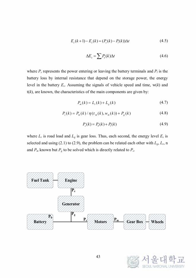
where Lr is road load and Lg is gear loss. Thus, each second, the energy level Es is

selected and using (2.1) to (2.9), the problem can be related each other with Lg, Lr, n

and Pm known but Pg to be solved which is directly related to Pe.

Battery

Fuel Tank Engine

Motors Gear Box Wheels

Pg

Pm

Pe

PsPb

Generator

44

Figure 4.3 Power Flow Relations

The fuel consumption rate can be expressed as a function of the engine

instantaneous generating power where w(k), t(k) is in OOL (Optimal Operating

Line):

m¢ = J(Pe(k)) (4.10)

by bsfc map each duration tD . And the current time t is tD ·k by discretization

parameter k. Thus, the cost function now becomes the fuel usage over the driving

cycle in the time interval using (4.2) and (4.10) as follows:

0

n

k

m t=

¢Då (4.11)

And all the optimization is achieved by single variable problem Pe in (4.10).

Therefore, by choosing appropriate Pe as a control variable, the characteristics of all

components included model would head for the optimal direction. This calculation

is from backward model and calculations worked out on the time interval of tD = 1

s, with Euler method [37].

The operating range of the components is limited, so more bounds have to be

set. This can be done by the following max, min constraints:

Pm,min ≤ Pm ≤ Pm,max (4.12)

Pe,min ≤ Pe ≤ Pe,max (4.13)

Pg,min ≤ Pg ≤ Pg,max (4.14)

Pb,min ≤ Pb ≤ Pb,max (4.15)

Es,min ≤ Es ≤ Es,max (4.16)

45

where motor power, engine power, generator power, battery power limitation and

the bounds on the battery energy level Es which is between 0 to 1 in SoC are

displayed and subscript min (max) means minimum (maximum). Finally, as the

endpoint constraint also is required. The energy level at the end of the cycle tf

would be the same as at the beginning as below:

( ) (0)s f sE t E= (4.17)

The optimization problem can be carried out using the variables and object

function relations above. However, nonlinear solvers are now necessary as the

optimization or minimization methodologies are not suggested above. The problem

minimization or optimization technique can be easily incorporated into an

optimization technique, such as DP. However, as the computation time is limited to

an online application, another nonlinear optimization solver QP (Quadratic Problem)

might be better. In fact, only a limited prediction of the future driving cycle would

be available and NLP with semi MPC structure was used as in the next Chapter

[72].

4.2.2 Dynamic Programming

Dynamic Programming is well known for global optimization technique and

basically solves an optimization problem with assumption of knowing all speed

information in advance [13, 73]. The time division and possible energy levels in DP

become as follows:

/fn t t= D (4.18)

,max ,min( ) /s s sl E E E= - D (4.19)

46

where n is the length of the driving cycle. Equations (4.10) define the instantaneous

fuel consumption of a dynamic system with the control input Pe, however in DP all

the calculation were worked out base on the battery power Pb, which has direct

relation with Es or SoC. The relation between sED and

bPD is:

s bE P tD = D ´D (4.20)

and Pcur matrix which contains the current information of each energy level in (4.19)

at that time is calculated and the possible the engine generating points considering

road load energy consumption and engine generating are found. The feasible input

at each instant k can be defined by Pb:

Pb,min ≤ u(k)D Pb≤ Pb,max (4.21)

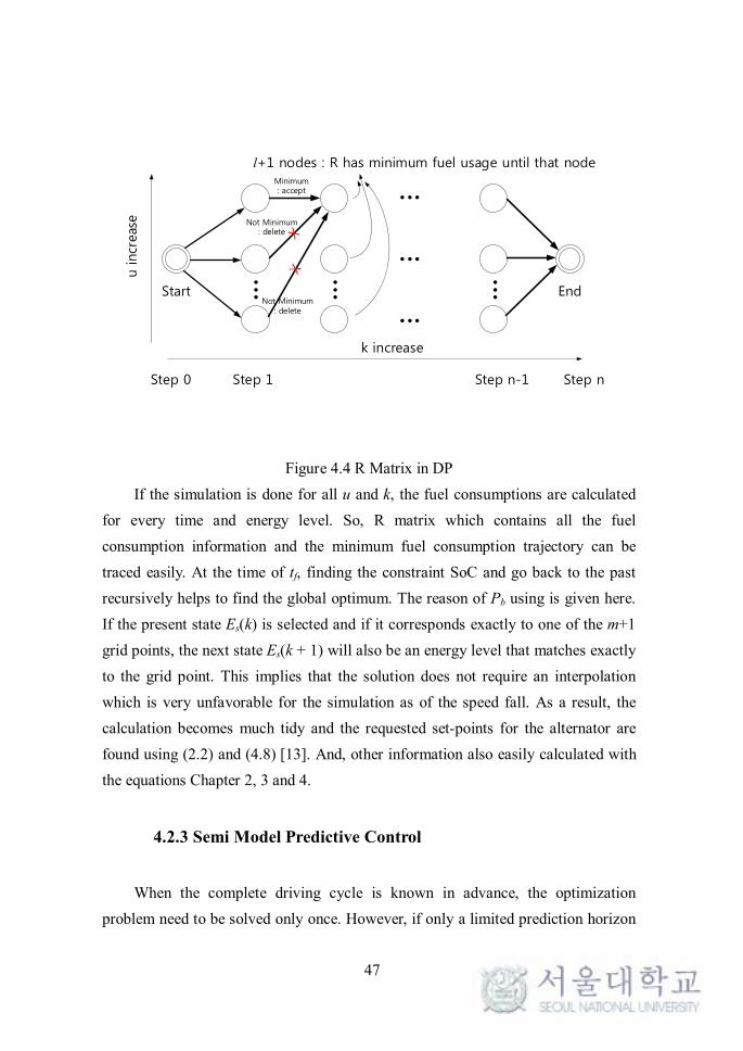
Therefore, it is possible to define a matrix R that possess the fuel consumption

information at all feasible combinations (u, k) for the given driving cycle. R

becomes (l+1) × n matrix and the minimum consumption at that time and that

battery energy level is saved as in Figure 4.4. That is, the fuel consumption is

evaluated and saved at every R(u,k), where u0 is the starting energy level constraint

of the battery [13, 74]:

R(0,u0)=0 (4.22)

47

Step 0 Step 1

k increase

Step n-1 Step n

...

...

...Start End

l+1 nodes : R has minimum fuel usage until that node

u incr

eas

e

Minimum: accept

Not Minimum: delete

Not Minimum: delete

... ......

Figure 4.4 R Matrix in DP

If the simulation is done for all u and k, the fuel consumptions are calculated

for every time and energy level. So, R matrix which contains all the fuel

consumption information and the minimum fuel consumption trajectory can be

traced easily. At the time of tf, finding the constraint SoC and go back to the past

recursively helps to find the global optimum. The reason of Pb using is given here.

If the present state Es(k) is selected and if it corresponds exactly to one of the m+1

grid points, the next state Es(k + 1) will also be an energy level that matches exactly

to the grid point. This implies that the solution does not require an interpolation

which is very unfavorable for the simulation as of the speed fall. As a result, the

calculation becomes much tidy and the requested set-points for the alternator are

found using (2.2) and (4.8) [13]. And, other information also easily calculated with

the equations Chapter 2, 3 and 4.

4.2.3 Semi Model Predictive Control

When the complete driving cycle is known in advance, the optimization

problem need to be solved only once. However, if only a limited prediction horizon

48

is available, the problem can solved by Model Predictive Control (MPC). This

methodology minimizes the object function at each time step over a limited

prediction horizon and extracts some control sequence. At the next time step, a new

optimization is then again carried out using an updated data [72, 75-77].

Basically, MPC is described by the formula as bellows:

2 2( )i i i i iJ w r x y u= - + Då å (4.23)

where xi is ith controlled variable and ri is ith reference variable. And wi and yi are

weighting factors which do the role of adjusting x importance and u variances. The

optimization cost function J in (4.23) is usually given by QP (quadratic problem) as

QP has a clear minimum point. So each sampling instant k, if we assume the time is

t, x(t+k/t) is computed for a certain horizon N, as functions of the control action

u(t+k/t).

MPC usually takes the first element of the optimal predicted input sequence:

u(k) = u*(t+k|t) (4.24)

The process of computing u(k) by minimizing the predicted cost and implementing

the first element of u* is then repeated at each sampling instant k with same:

k= [0 … N] (4.25)

Nt0 = Nt1 … = Np (4.26)

where Np is the final receding horizon for MPC. Therefore, the strategy becomes an

online optimization strategy and the prediction horizon remains same length as

Figure 4.5. By continually shifting the horizon, this horizon can be continued

infinitely.

49

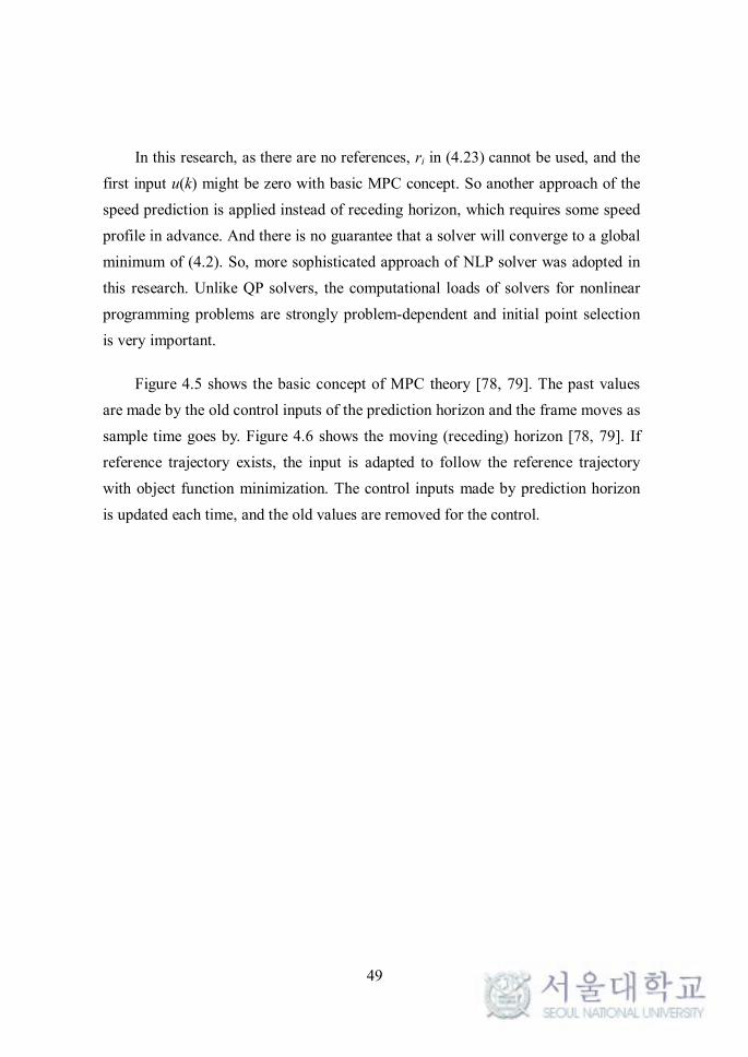
In this research, as there are no references, ri in (4.23) cannot be used, and the

first input u(k) might be zero with basic MPC concept. So another approach of the

speed prediction is applied instead of receding horizon, which requires some speed

profile in advance. And there is no guarantee that a solver will converge to a global

minimum of (4.2). So, more sophisticated approach of NLP solver was adopted in

this research. Unlike QP solvers, the computational loads of solvers for nonlinear

programming problems are strongly problem-dependent and initial point selection

is very important.

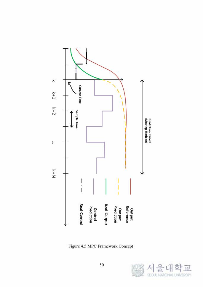
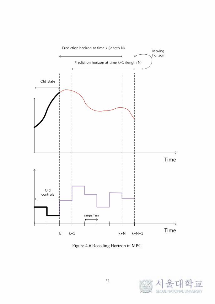
Figure 4.5 shows the basic concept of MPC theory [78, 79]. The past values

are made by the old control inputs of the prediction horizon and the frame moves as

sample time goes by. Figure 4.6 shows the moving (receding) horizon [78, 79]. If

reference trajectory exists, the input is adapted to follow the reference trajectory

with object function minimization. The control inputs made by prediction horizon

is updated each time, and the old values are removed for the control.

50

kk+1

k+

2k+N

...

Outp

ut

Refe

rence

Outp

ut

Pre

dictio

n

Real O

utp

ut

Contro

l Pre

dictio

n

Sam

ple

Tim

e

Real C

ontro

l

Pre

dictio

n P

erio

d

(Movin

g H

oriz

on)

Curre

nt T

ime

Figure 4.5 MPC Framework Concept

51

k k+1 k+N+1

Sample Time

Time

Time

k+N

Prediction horizon at time k (length N)

Prediction horizon at time k+1 (length N)

Old controls

Old state

Moving horizon

Figure 4.6 Receding Horizon in MPC

52

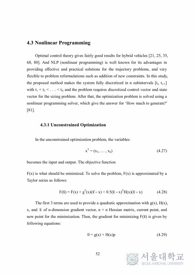
4.3 Nonlinear Programming

Optimal control theory gives fairly good results for hybrid vehicles [21, 25, 35,

68, 80]. And NLP (nonlinear programming) is well known for its advantages in

providing effective and practical solutions for the trajectory problems, and very

flexible to problem reformulations such as addition of new constraints. In this study,

the proposed method makes the system fully discretized in n subintervals [ti, ti+1]

with t1 < t2 < . . . < tf, and the problem requires discretized control vector and state

vector for the sizing problem. After that, the optimization problem is solved using a

nonlinear programming solver, which give the answer for ‘How much to generate?’

[81].

4.3.1 Unconstrained Optimization

In the unconstrained optimization problem, the variables:

xT = (x1, … , xn) (4.27)

becomes the input and output. The objective function

F(x) is what should be minimized. To solve the problem, F(x) is approximated by a

Taylor series as follows:

F(x ) = F(x) + gT(x)(x –x) + 0.5(x –x)TH(x)(x –x) (4.28)

The first 3 terms are used to provide a quadratic approximation with g(x), H(x),

x, and x of n-dimension gradient vector, n × n Hessian matrix, current point, and

new point for the minimization. Then, the gradient for minimizing F(x ) is given by

following equations:

0 = g(x) + H(x)p (4.29)

53

P = x – x (4.30)

P = -H-1(x)g(x) (4.31)

4.3.2 Equality Constraints

If m-constraints of c(x) = 0 subject to m < n are used in the problem, Lagrange

multipliers are required and the problem becomes:

L(x, λ) = F(x) – λTc(x) (4.32)

And at the optimal values of (x*, λ*), the constraints satisfy following conditions

[81]:

▽x L(x*, λ*) = 0 (4.33)

▽λ L(x*, λ*) = 0 (4.44)

And the gradient of L with respect to x or λ become as follows:

▽x L = g – GTλ (G = ∂c/∂x, Jacobian) (4.45)

▽λ L = -c(x) (4.46)

In fact, the real x and λ update to accomplish (4.45), (4.46) is achieved by 3-term

Taylor series expansion of (4.47), (4.48) about (x, λ) and are obtained by:

0 = g – GTλ + HL(x – x) – GT(λ – λ) (4.47)

0 = -c – G(x –x) (4.48)

where HL is the Hessian of the Lagrangian and λ is the vector of Lagrange

multipliers at the new point. Now the system can be simplified as bellows and

called KKT (Karush-Kuhn-Tucker) condition:

54

TL

-p gH G=

λ cG 0

é ù é ù é ùê ú ê ú ê ú

ë û ë ûë û (4.49)

As (4.49) gives the direction to the minimization, the appropriate variable direction

for the convergence can be calculated.

4.3.3 Inequality Constrains

If the inequality constraints of λi(x) ≥ 0 is used, the system distinguishes

whether ith λi(x) is active or not. If λi(x) is active that λi(x*) = 0 then, the

problem considers the inequality constraint just as it considers the equality

condition. But if λi(x*) > 0, it is called inactive and removed from the calculation

[81].

4.3.4 SQP (Sequential Quadratic Programming)

Equation (4.27) to (4.49) shows the process how to solve the complex problem

by quadratic approximation and recursive updates [82]. In NLP theory, F(x) solving

problem becomes quadratic programming problem and the minimum is found with

the selective choices of inequality conditions not to violate any inactive inequalities.

With such recursive updates, the problem converges and stops optimization. Then,

it starts the same process at the minimum point again. In other words, perform (4.27)

to (4.49) and finds the minimum again and again until the value is assumed to the

sub-global minimum by NLP theory where lots of globalization strategies can be

used. In the problem, the workstation CPU of 3.3 gHz and nonlinear programming

solver ‘NPSOL’ was used each 1 s time interval to achieve that [81].

4.3.5 Problem Reconstruction

55

With the NLP theory, the problem object is to minimize the total fuel

consumption during the cycle and can be summarized as follows:

k = 1 , … , 776 (total 776 seconds)

P = [p1, p2, p3,…, p776] (kW, control variables) (4.50)

SOC = [SoC1, SoC2, SoC3,…, SoC776] (%, state variables) (4.51)

where [P, SOC] becomes NLP inputs. And the constraints are:

SOC(t0) = SoCinit (4.52)

SOC(tf) = SoCfin (4.53)

SoC − SoC = ( , ,

(4.54)

tD =1 (4.55)

Minimum Motor Power ≤ Motor Power ≤ Maximum Motor Power (4.56)

Minimum Generator Power ≤ Generator Power ≤ 0 (4.57)

0 (kW) ≤ Engine Power ≤ Maximum Engine Power (4.58)

Minimum Battery Current ≤ Battery Current Limit ≤ Maximum Battery Current (4.59)

Minimum Motor Torque ≤ Motor Torque ≤ Maximum Motor Torque (4.60)

Minimum Generator Torque ≤ Generator Torque ≤ Maximum Generator Torque (4.61)

Minimum Engine Torque ≤ Engine Torque ≤ Maximum Engine Torque (4.62)

56

where SoCinit and SoCfin are initial and final SoC and the initial SoC and final SoC

are same to evaluate the exact fuel effects as hybrid vehicle can operate by the

battery only. And equation (4.54) should be satisfied each time [83, 84]:

1( ) ( )( ) ( )

tk kx t x td

x t x tdt

+ -= »

D& (4.63)

NLP requires a boundary condition of SoC such that the monthly average SoC

of the same driver’s bus was used. And as the velocity prediction of the bus running

route is required, in the next Chapter, the velocity prediction method is suggested.

4.3.6 NLP Starting Point Selections

Usually, solution by NLP makes sinks to local minimum, so finding the

appropriate starting points is very important. In this problem, the control parameter

input is:

Parameter = [par1, par2, par3 … parn] (4.64)

and the problem is ‘When to generate?’. It is mostly affected by the efficiency of

the battery. The required power in front of the battery, Ps, is determined by the road

load and Figure 4.7(a) shows the key to that issue as it shows the standard of ‘when

to generate’. The battery efficiency varies according Ps as the output of the battery

is total energy vs. loss subtracted total energy. (Battery Efficiency, Required Power

ahead the Battery) becomes (0.95, 48.5kW), (0.93, 66.45kW), (0.9, 91.87kW),

(0.87, (115.4kW), and (0.85, 130 kW), and it would be more favorable of engine

generating when the battery efficiency is low. In Figure 2.8, the best bsfc generating

becomes much more efficient than other OOL points and it would be easily known

that usually this bus cycle does not requires much over 130 kW as in Figure 4.7(b),

and the forced generation over battery 0.95 is useless as the battery efficiency is too

high. Therefore, 3 points of (0.95, 0.9, 0.85) and (48.5 kW, 91.9 kW, 130.1 kW)

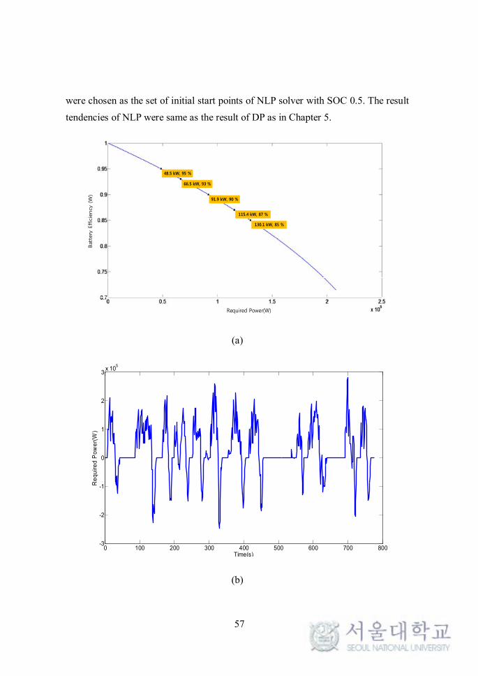
57

were chosen as the set of initial start points of NLP solver with SOC 0.5. The result

tendencies of NLP were same as the result of DP as in Chapter 5.

66.5 kW, 93 %

48.5 kW, 95 %

91.9 kW, 90 %

115.4 kW, 87 %

130.1 kW, 85 %

Required Power(W)

Batt

ery

Effic

iency

(W

)

(a)

(b)

0 100 200 300 400 500 600 700 800-3

-2

-1

0

1

2

3x 10

5

Time(s)

Re

qu

ire

d P

ow

er(

W)

58

Figure 4.7 Initial Point Selections by Battery Efficiency (a) Battery Efficiency with

the Required Power (b) Required Power at the Battery

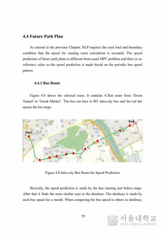
59

4.4 Future Path Plan

As uttered in the previous Chapter, NLP requires the road load and boundary

condition that the speed for running route calculation is essential. The speed

prediction of future path plane is different from usual MPC problem and there is no

reference value so the speed prediction is made based on the periodic bus speed

pattern.

4.4.1 Bus Route

Figure 4.8 shows the selected route. It contains 4.3km route from ‘Ilwon

Tunnel’ to ‘Garak Market’. The bus run here is 401 intra-city bus and the red dot

means the bus stops.

Start

End

Figure 4.8 Intra-city Bus Route for Speed Prediction

Basically, the speed prediction is made by the bus running just before stops.

After that it finds the most similar case in the database. The database is made by

each bus speed for a month. When comparing the bus speed to others in database,

60

the speed comparison comparing ‘Speed vs. Time’ is not possible as of the

deviation of time at the same spot. Figure 4.9 shows the speed according to time.

Thus another approach is required and ‘Speed vs. Distance’ is a solution in Figure

4.10, because every bus are suggested to stop at a bus stop.

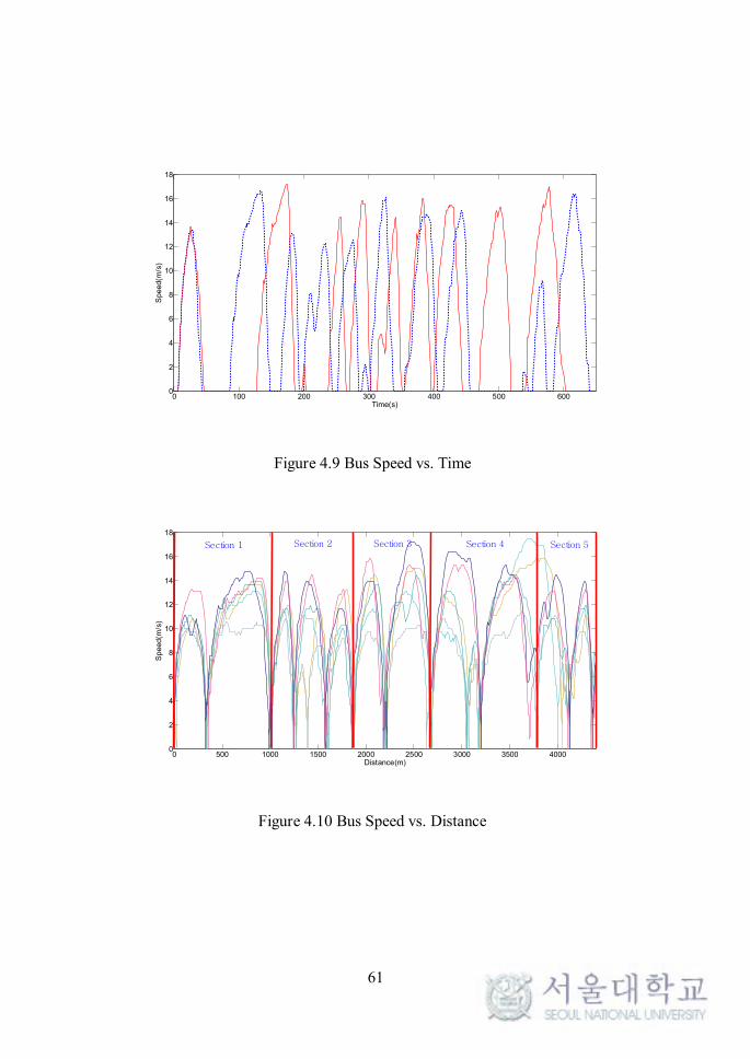
61

Figure 4.9 Bus Speed vs. Time

Figure 4.10 Bus Speed vs. Distance

0 100 200 300 400 500 6000

2

4

6

8

10

12

14

16

18

Time(s)

Speed(m

/s)

0 500 1000 1500 2000 2500 3000 3500 40000

2

4

6

8

10

12

14

16

18

Distance(m)

Speed(m

/s)

Section 1 Section 2 Section 3 Section 4 Section 5

62

4.4.2 Speed Prediction Algorithm

The basic algorithm of speed prediction is in Figure 4.11. To expect the speed

of section 2, run section 1 and find the most similar speed cases based on ‘Speed vs.

Distance’ comparison. As the similar speed means similar traffic conditions. If the

run speed is same at the same distance, the traffic or traffic signals would be similar.

The similar cases are found by:

2[ ( ) ( )]m

refv i v i-å (4.65)

where v(i) and vref(i) is the velocity in each distance. To achieve that the database

for the vehicle speed should be made by speed vs distance.

Now, the similar 5 cases are found. Then, as the bus has run section 1 so the

duration time for the section 1 can be known. And the next section duration time

will be given by Seoul Transport Operation & Information Service. So the time can

be assumed to be used (next time duration is usually given nowadays by a smart

phone). Thus the finding timing becomes:

T1 = Time to next section start by information service (4.66)

T2 = Time to next section start by data base (4.67)

T1 » T2 (4.68)

The reason of finding (4.68) is that if the speed and time similar, the traffic

condition seems to be similar. As a result, the next session is made by this way as

MPC does this with receding horizon. And the expected speed can be synched by

speed zero to positive case. The result is in Figure 4.12. The most important thing

about the speed expectation is that the traffic jam should not be so harsh. And the

database should be made one driver as the driving style is totally different

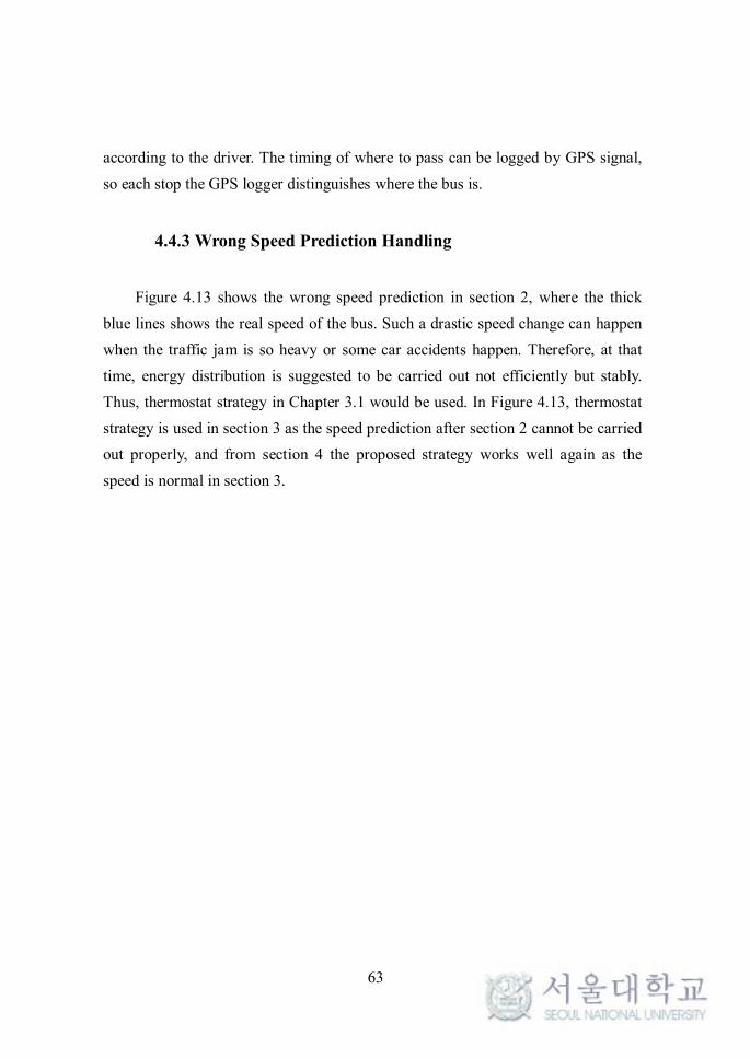
63

according to the driver. The timing of where to pass can be logged by GPS signal,

so each stop the GPS logger distinguishes where the bus is.

4.4.3 Wrong Speed Prediction Handling

Figure 4.13 shows the wrong speed prediction in section 2, where the thick

blue lines shows the real speed of the bus. Such a drastic speed change can happen

when the traffic jam is so heavy or some car accidents happen. Therefore, at that

time, energy distribution is suggested to be carried out not efficiently but stably.

Thus, thermostat strategy in Chapter 3.1 would be used. In Figure 4.13, thermostat

strategy is used in section 3 as the speed prediction after section 2 cannot be carried

out properly, and from section 4 the proposed strategy works well again as the

speed is normal in section 3.

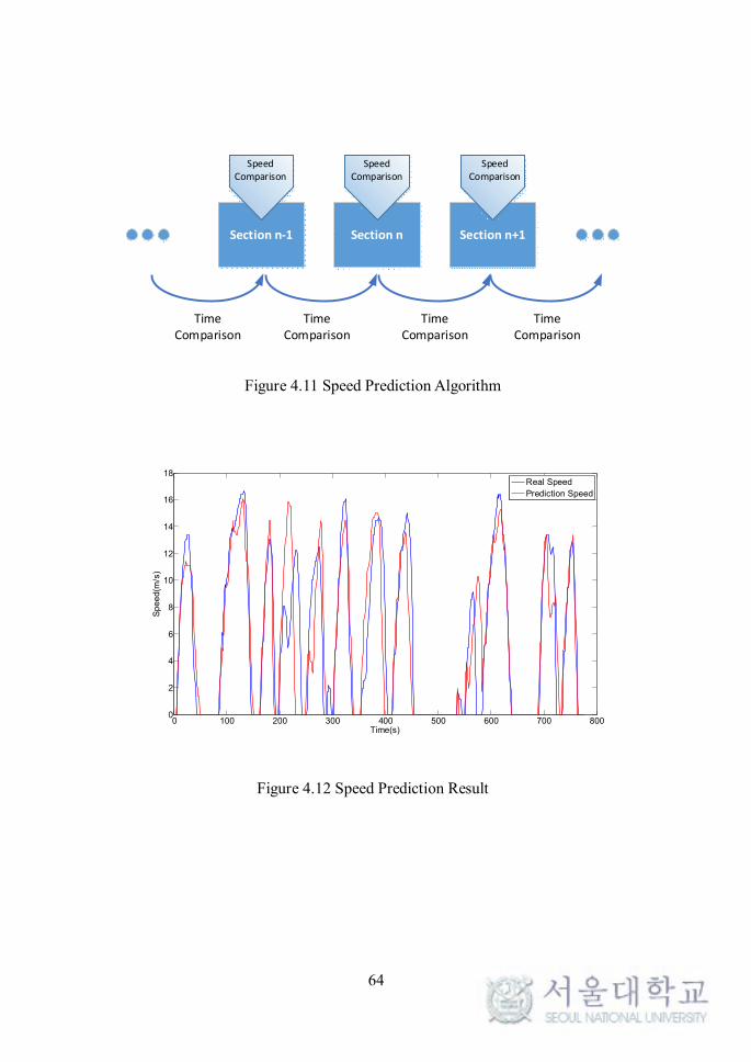
64

Section n-1 Section n Section n+1

Speed Comparison

Speed Comparison

Speed Comparison

Time Comparison

Time Comparison

Time Comparison

Time Comparison

Figure 4.11 Speed Prediction Algorithm

Figure 4.12 Speed Prediction Result

0 100 200 300 400 500 600 700 8000

2

4

6

8

10

12

14

16

18

Time(s)

Sp

ee

d(m

/s)

Real Speed

Prediction Speed

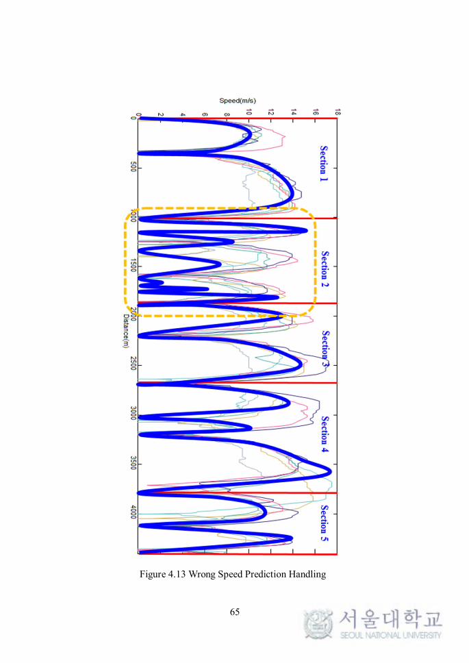
65

Figure 4.13 Wrong Speed Prediction Handling

66

4.5 Signal Manipulation

This Chapter introduces some techniques which improve the fuel economy.

The additional techniques contain the signal synchronization, signal bundle

transmitting, signal removing and filling, and zero speed synchronization.

4.5.1 Signal Synchronization

Basically the speed prediction finds the most similar speed at the next session.

However, Figure 4.14 shows the speed prediction result comparison, and even

though the speed prediction is very good, the synchronization is another problem.

In Figure 4.15, the bar-type signal is engine command signal after NLP calculation.

Even though the magnitude difference is same (well predicted), if it does not

happen at the appropriate time, the speed prediction would be useless as in SHEV,

‘When to generate?’ is the problem of the synchronization. Therefore, after NLP

finding the command signal in each semi MPC frame, the command signal was

transmitted only when the speed 0 to positive value transition happens. That’s

because at the transition, the compulsory generation starts caused by the battery

efficiency. This will be happen at every velocity transition 0 to positive transition,

so even though the velocity prediction was right but not synchronized, the wrong

synchronized signal problem would be far diminished. This is uniquely adaptable to

series type hybrid electric vehicle, as the engine/generator unit works independently

from the traction motor.

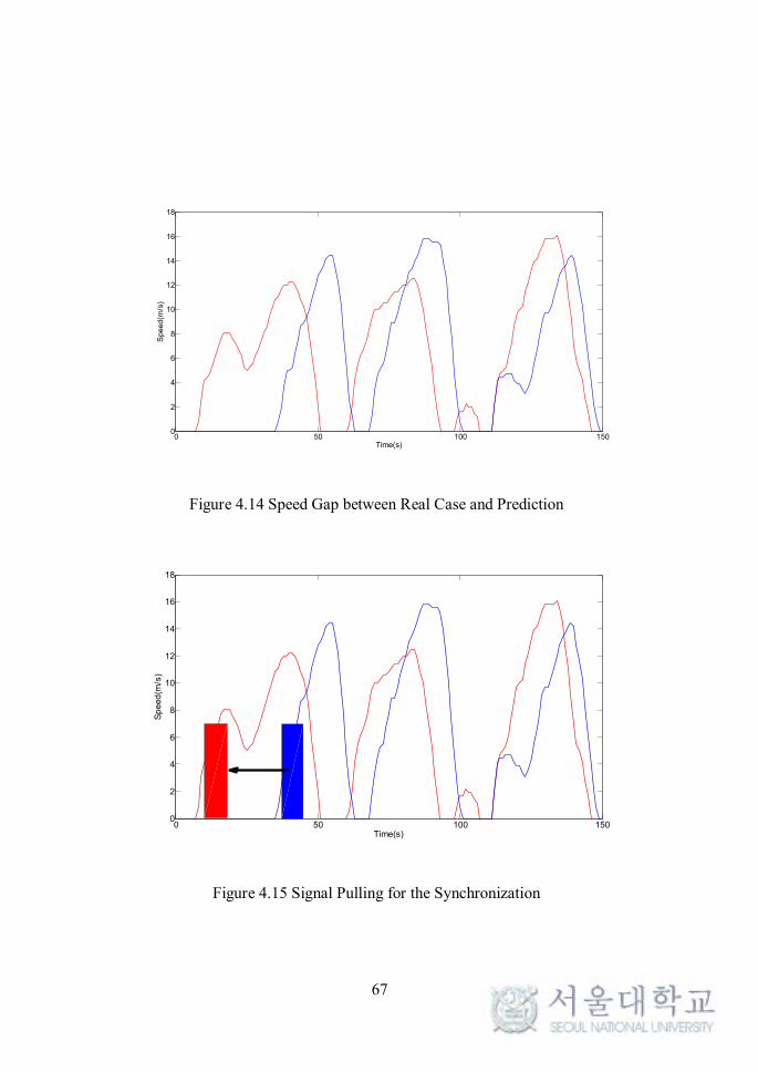
67

Figure 4.14 Speed Gap between Real Case and Prediction

Figure 4.15 Signal Pulling for the Synchronization

0 50 100 1500

2

4

6

8

10

12

14

16

18

Time(s)

Speed(m

/s)

0 50 100 1500

2

4

6

8

10

12

14

16

18

Time(s)

Sp

ee

d(m

/s)

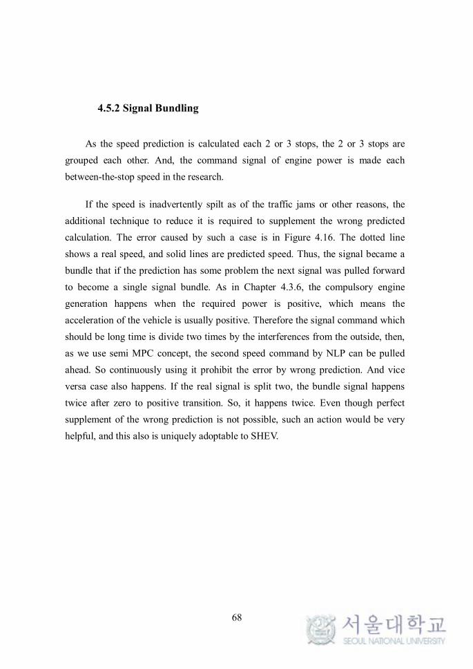
68

4.5.2 Signal Bundling

As the speed prediction is calculated each 2 or 3 stops, the 2 or 3 stops are

grouped each other. And, the command signal of engine power is made each

between-the-stop speed in the research.

If the speed is inadvertently spilt as of the traffic jams or other reasons, the

additional technique to reduce it is required to supplement the wrong predicted

calculation. The error caused by such a case is in Figure 4.16. The dotted line

shows a real speed, and solid lines are predicted speed. Thus, the signal became a

bundle that if the prediction has some problem the next signal was pulled forward

to become a single signal bundle. As in Chapter 4.3.6, the compulsory engine

generation happens when the required power is positive, which means the

acceleration of the vehicle is usually positive. Therefore the signal command which

should be long time is divide two times by the interferences from the outside, then,

as we use semi MPC concept, the second speed command by NLP can be pulled

ahead. So continuously using it prohibit the error by wrong prediction. And vice

versa case also happens. If the real signal is split two, the bundle signal happens

twice after zero to positive transition. So, it happens twice. Even though perfect

supplement of the wrong prediction is not possible, such an action would be very

helpful, and this also is uniquely adoptable to SHEV.

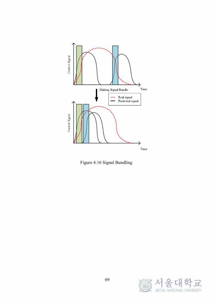
69

Figure 4.16 Signal Bundling

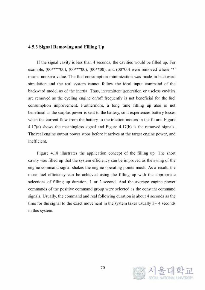
70

4.5.3 Signal Removing and Filling Up

If the signal cavity is less than 4 seconds, the cavities would be filled up. For

example, (00****00), (00***00), (00**00), and (00*00) were removed where ‘*’

means nonzero value. The fuel consumption minimization was made in backward

simulation and the real system cannot follow the ideal input command of the

backward model as of the inertia. Thus, intermittent generation or useless cavities

are removed as the cycling engine on/off frequently is not beneficial for the fuel

consumption improvement. Furthermore, a long time filling up also is not

beneficial as the surplus power is sent to the battery, so it experiences battery losses

when the current flow from the battery to the traction motors in the future. Figure

4.17(a) shows the meaningless signal and Figure 4.17(b) is the removed signals.

The real engine output power stops before it arrives at the target engine power, and

inefficient.

Figure 4.18 illustrates the application concept of the filling up. The short

cavity was filled up that the system efficiency can be improved as the swing of the

engine command signal shakes the engine operating points much. As a result, the

more fuel efficiency can be achieved using the filling up with the appropriate

selections of filling up duration, 1 or 2 second. And the average engine power

commands of the positive command group were selected as the constant command

signals. Usually, the command and real following duration is about 4 seconds as the

time for the signal to the exact movement in the system takes usually 3~ 4 seconds

in this system.

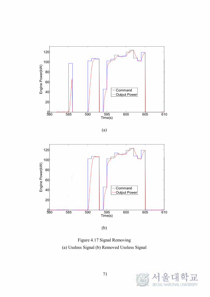
71

(a)

(b)

Figure 4.17 Signal Removing

(a) Useless Signal (b) Removed Useless Signal

580 585 590 595 600 605 6100

20

40

60

80

100

120

Time(s)

En

gin

e P

ow

er(

kW

)

CommandOutput Power

580 585 590 595 600 605 6100

20

40

60

80

100

120

Time(s)

En

gin

e P

ow

er(

kW

)

CommandOutput Power

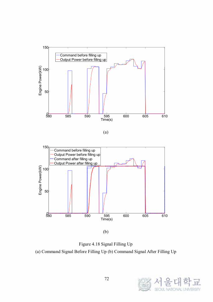
72

(a)

(b)

Figure 4.18 Signal Filling Up

(a) Command Signal Before Filling Up (b) Command Signal After Filling Up

580 585 590 595 600 605 6100

50

100

150

Time(s)

Eng

ine

Po

wer(

kW

)

Command before filling upOutput Power before filling up

580 585 590 595 600 605 6100

50

100

150

Time(s)

Eng

ine

Po

wer(

kW

)

Command before filling upOutput Power before filling upCommand after filling upOutput Power after filling up

73

4.5.4 Zero Speed Synchronization

As the explanation in Chapter 4.3.6, to use battery only is less efficient if the

required power is large, as of the battery efficiency, Vbus/Eoc. This also is applied to

the zero speed. When the required power is zero, it is better to generate the

engine/generator during the load happening as in Figure 4.7. Therefore, if the

required power is zero, engine power also engaged to be zero, which is shown in

the Chapter 5.1.3.

74

4.6 Motor Torque Distribution in MCU

In the past, when the MCU (Motor Control Unit) sent a total traction torque

command to the motors, the command was divided into two equal loads that were

sent to each traction motor. However, such a torque (power) distribution did not

consider the operating efficiency, unlike the proposed strategy, which includes

considerations for the efficiency using an optimal torque distribution map. The

MCU selects the best distribution at each operating point, and the torque is

distributed according to that map information.

4.6.1 Existing Strategy

The strategy for the basic power distribution in the traction motors was to split

the command torque from the MCU, as shown in Figure 4.19. For example, when

the torque command is 100 Nm, then a command of 50 Nm goes to traction motor 1

and to traction motor 2. This concept is very straightforward and universal in many

series hybrid vehicles [69, 85]. However, even though the power flow that starts

from the battery or the generator is optimal, it cannot be transferred to the wheels

via both traction motors in the most efficient manner.

4.6.2 Strategy Concept

The proposed strategy identifies the optimal distribution at each operating

point. When the torque signal is sent from the MCU, the distribution is carried out

with the pre-calculated optimal torque distribution map. To find the optimal point

of the power distribution, the total T-N curve (the sum of the two maximum motor

torques) for the torque distribution, as shown in Figure 4.20, is essential. In this

research, because the two motors are the same, the RPM limit is the same, and the

maximum torque is doubled. The approach for achieving the best efficiency is

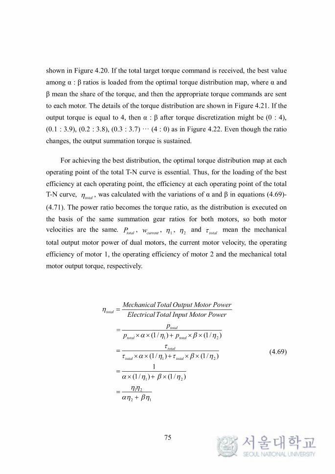
75

shown in Figure 4.20. If the total target torque command is received, the best value

among α : β ratios is loaded from the optimal torque distribution map, where α and

β mean the share of the torque, and then the appropriate torque commands are sent

to each motor. The details of the torque distribution are shown in Figure 4.21. If the

output torque is equal to 4, then α : β after torque discretization might be (0 : 4),

(0.1 : 3.9), (0.2 : 3.8), (0.3 : 3.7) ··· (4 : 0) as in Figure 4.22. Even though the ratio

changes, the output summation torque is sustained.

For achieving the best distribution, the optimal torque distribution map at each

operating point of the total T-N curve is essential. Thus, for the loading of the best

efficiency at each operating point, the efficiency at each operating point of the total

T-N curve, totalh , was calculated with the variations of α and β in equations (4.69)-

(4.71). The power ratio becomes the torque ratio, as the distribution is executed on

the basis of the same summation gear ratios for both motors, so both motor

velocities are the same. totalP ,

currentw , 1h ,

2h and totalt mean the mechanical

total output motor power of dual motors, the current motor velocity, the operating

efficiency of motor 1, the operating efficiency of motor 2 and the mechanical total

motor output torque, respectively.

1 2

1 2

1 2

1 2

2 1

(1/ ) (1/ )

(1/ ) (1/ )

1

(1/ ) (1/ )

total

total

total total

total

total total

Mechanical Total Output Motor Power

ElectricalTotal Input Motor Power

p

p p

h

a h b h

t

t a h t b h

a h b h

hh

ah bh

=

=´ ´ + ´ ´

=´ ´ + ´ ´

=´ + ´

=+

(4.69)

76

total total currentp wt= ´ (4.70)

1a b+ = (4.71)

The efficiency in equation (4.69) is compared with each variation of the

operating point (α and β), and as in equation (4.72), the maximum value is saved to

the optimal torque distribution map,_total besth , at each operating point with the

information of α and β.

_ max( )total best totalh h= (4.72)

Thus, at each operating point, the best ratio can be found, and the results can

be saved in the total T-N curve operating region.

4.6.3 Procedure

The procedure for making the optimal torque distribution map is outlined in

Figure 4.23. Because the ratio α : β was optimized after discretization, it is

advantageous as the subdivision is delicate. The optimal torque distribution map

becomes symmetric about the x-axis (generating mode).

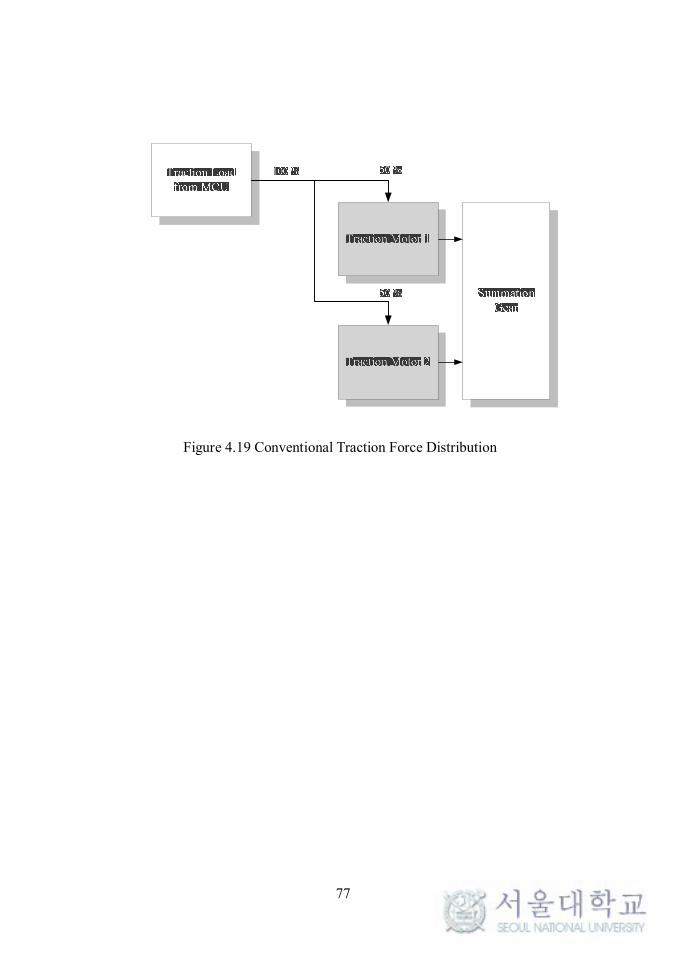
77

Figure 4.19 Conventional Traction Force Distribution

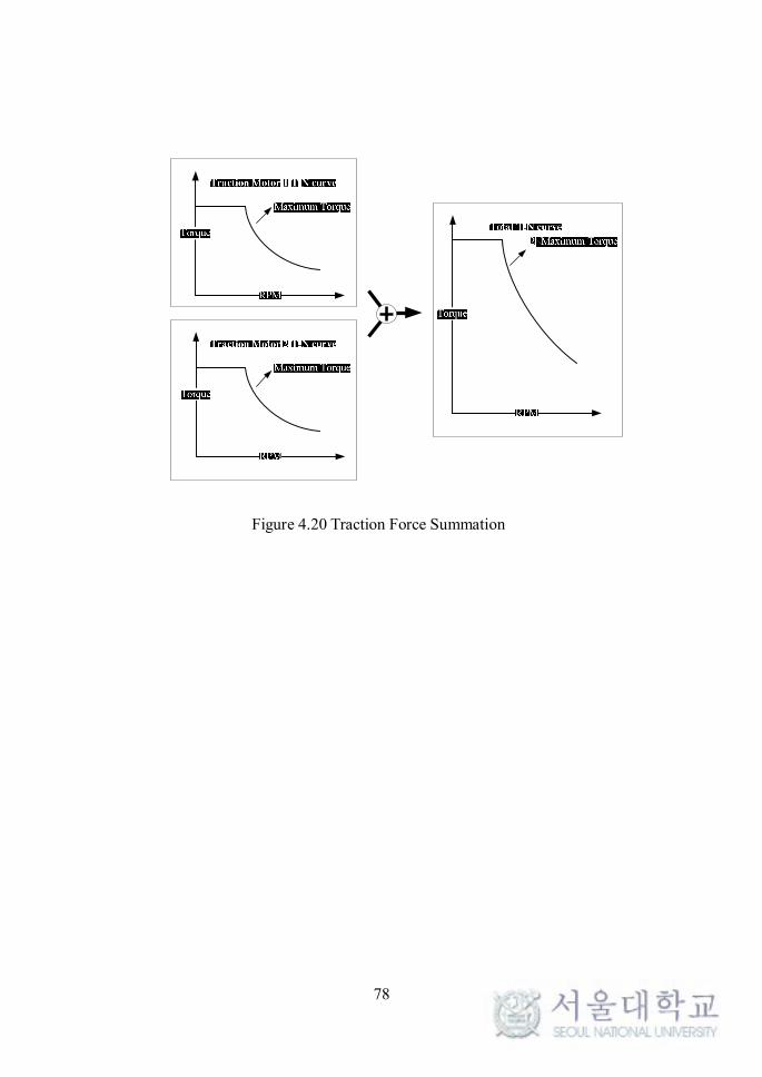
78

Figure 4.20 Traction Force Summation

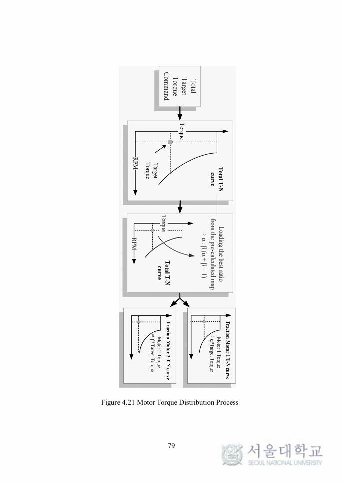
79

Figure 4.21 Motor Torque Distribution Process

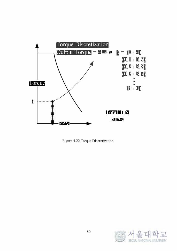
80

…

Figure 4.22 Torque Discretization

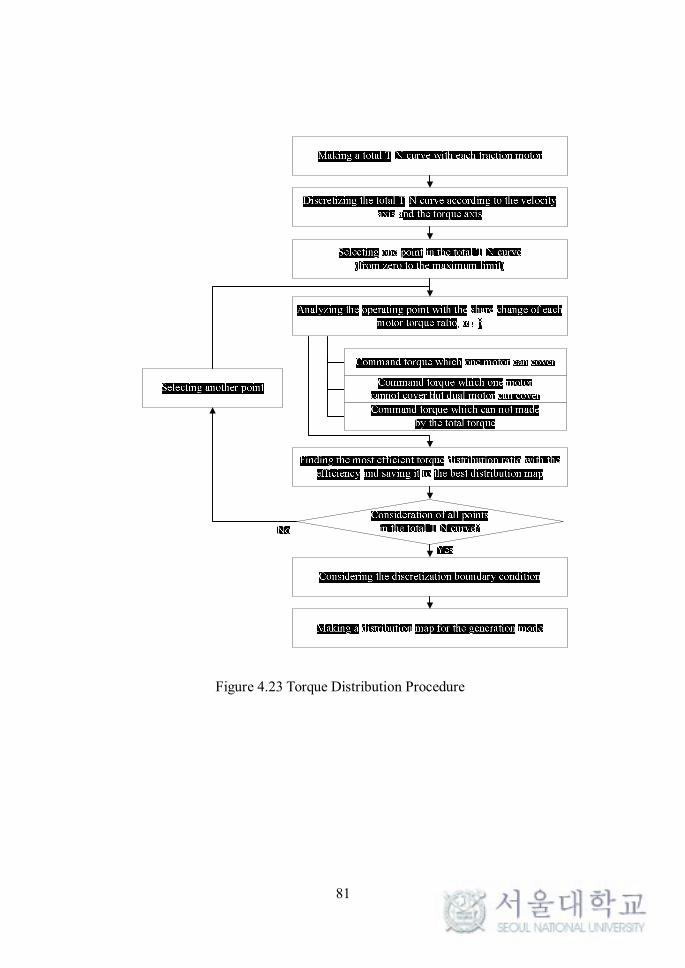
81

Figure 4.23 Torque Distribution Procedure

82

Chapter 5. Simulation Results

The basic questions of the result is ‘Does the NLP result follows DP result

well?’, ‘Can it be improved?’ and ‘Torque distribution is really effective?’. First, if

the result by the proposed strategy follows that of DP, the calculation accuracy is

reliable. Second and third, the improvement can be proved by signal manipulation

and torque distribution and they can be verified by the fuel consumption

improvement. In this chapter, the control input is engine generating power, and the

state variable is the battery state of charge, and object function is total fuel

consumption. All evaluations are carried out and compared to DP result which is

the reference for all evaluations.

5.1 Engine Generating Power

Figure 5.1 and 5.2 shows the control input by two cases. The important

considerations are timing and engine generation power. As in the Figure 5.3, two

cases overlap much that the prediction by NLP is reliable. Furthermore, the

generation power is also very similar. As in Figure 2.7(b), the best bsfc is found

near 103 kW and it affects the generation directly. The efficiency in the generator is

high in almost all area so the engine bsfc map becomes a critical key to the

generation efficiency. Figure 5.4 shows the zoomed area of Figure 5.3. In the figure,

the case fits well but, in the real vehicle propulsion, the speed was not usual case of

parabola type (usual speed trajectory would be parabola in one stop at the bus

route). Such a case happens when the sudden brake happens in the bus as in Figure

5.5. If the bus speed is normal with periodicity and the road traffic is not heavy, the

cases would not occur and NLP result would be well matched with DP result all the

time. These outputs are from backward model and reused as an input command to

the forward model immediately. Hereafter, the word MPC in the figure means the

83

result by proposed strategy where the word ‘semi’ in front of MPC was omitted as a

matter of convenience.

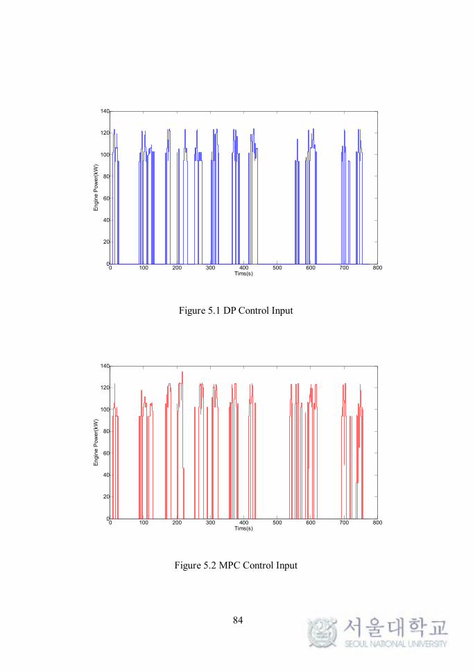
84

Figure 5.1 DP Control Input

Figure 5.2 MPC Control Input

0 100 200 300 400 500 600 700 8000

20

40

60

80

100

120

140

Tims(s)

En

gin

e P

ow

er(

kW

)

0 100 200 300 400 500 600 700 8000

20

40

60

80

100

120

140

Tims(s)

En

gin

e P

ow

er(

kW

)

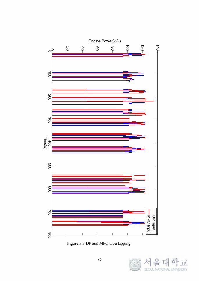
85

Figure 5.3 DP and MPC Overlapping

010

02

00

30

040

05

00

60

07

00

80

00

20

40

60

80

10

0

12

0

14

0

Tim

s(s

)

Engine Power(kW)

DP

Inp

ut

MP

C In

pu

t

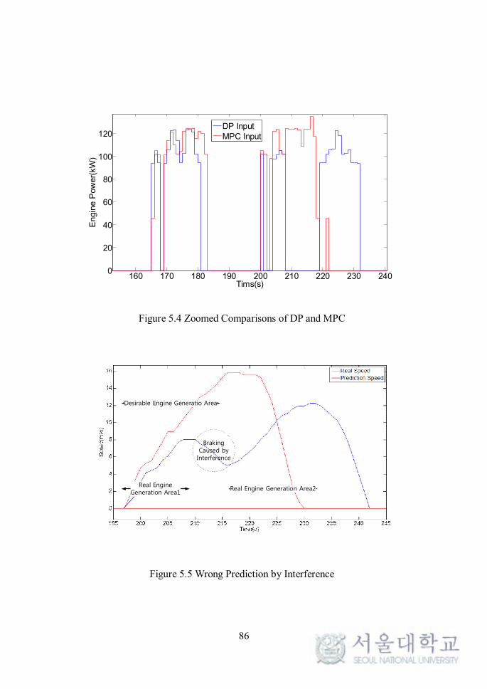
86

Figure 5.4 Zoomed Comparisons of DP and MPC

Desirable Engine Generatio Area

Real Engine Generation Area1

Real Engine Generation Area2

Braking Caused by Interference

Figure 5.5 Wrong Prediction by Interference

160 170 180 190 200 210 220 230 2400

20

40

60

80

100

120

Tims(s)

Engin

e P

ow

er(

kW

)

DP InputMPC Input

87

88

5.2 Battery SoC (State of Charge)

Figure 5.6 shows the power generation by thermostat strategy and power

follower strategy and the result SoC is in Figure 5.7. Thermostat strategy turn on

the engine when SoC becomes lower than the lower boundary value and stop

generating when it meets the upper boundary value. On the contrary, power

follower strategy tries to keep SoC, so it generate according to the load and the

drastic SoC change does not happen.

Figure 5.7 shows the SoC changes. The biggest gap is given among them by

thermostatic strategy. That’s because the generation standards is totally different

from that of DP or MPC. The result by DP and MPC is very similar each other, so

the proposed strategy reliability could be confirmed.

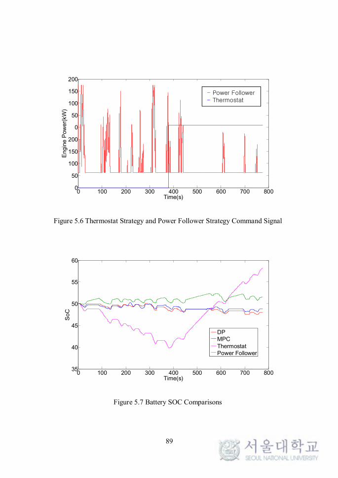
89

Figure 5.6 Thermostat Strategy and Power Follower Strategy Command Signal

Figure 5.7 Battery SOC Comparisons

0 100 200 300 400 500 600 700 8000

50

100

150

200

0

50

100

150

200

Time(s)

Engin

e P

ow

er(

kW

)

0 100 200 300 400 500 600 700 80035

40

45

50

55

60

Time(s)

So

C

DPMPCThermostatPower Follower

- Power Follower - Thermostat

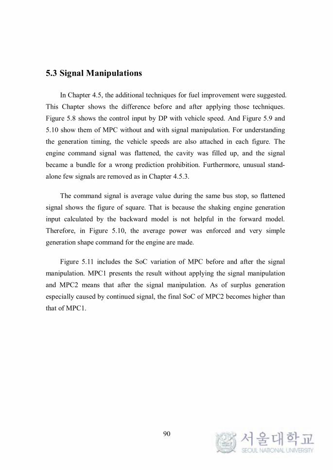
90

5.3 Signal Manipulations

In Chapter 4.5, the additional techniques for fuel improvement were suggested.

This Chapter shows the difference before and after applying those techniques.

Figure 5.8 shows the control input by DP with vehicle speed. And Figure 5.9 and

5.10 show them of MPC without and with signal manipulation. For understanding

the generation timing, the vehicle speeds are also attached in each figure. The

engine command signal was flattened, the cavity was filled up, and the signal

became a bundle for a wrong prediction prohibition. Furthermore, unusual stand-

alone few signals are removed as in Chapter 4.5.3.

The command signal is average value during the same bus stop, so flattened

signal shows the figure of square. That is because the shaking engine generation

input calculated by the backward model is not helpful in the forward model.

Therefore, in Figure 5.10, the average power was enforced and very simple

generation shape command for the engine are made.

Figure 5.11 includes the SoC variation of MPC before and after the signal

manipulation. MPC1 presents the result without applying the signal manipulation

and MPC2 means that after the signal manipulation. As of surplus generation

especially caused by continued signal, the final SoC of MPC2 becomes higher than

that of MPC1.

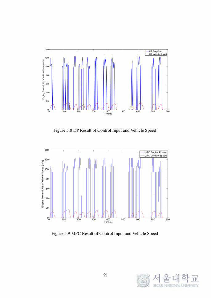
91

Figure 5.8 DP Result of Control Input and Vehicle Speed

Figure 5.9 MPC Result of Control Input and Vehicle Speed

0 100 200 300 400 500 600 700 8000

20

40

60

80

100

120

140

X: 540Y: 1.389

Time(s)

Engin

g P

ow

er(

kW

) or

Ve

hic

le S

peed(m

/s)

DP Eng Pow

DP Vehicle Speed

0 100 200 300 400 500 600 700 8000

20

40

60

80

100

120

140

Time(s)

En

gin

e P

ow

er

(kW

) o

r V

eh

icle

Sp

ee

d (

m/s

)

MPC Engine Power

MPC Vehicle Speed

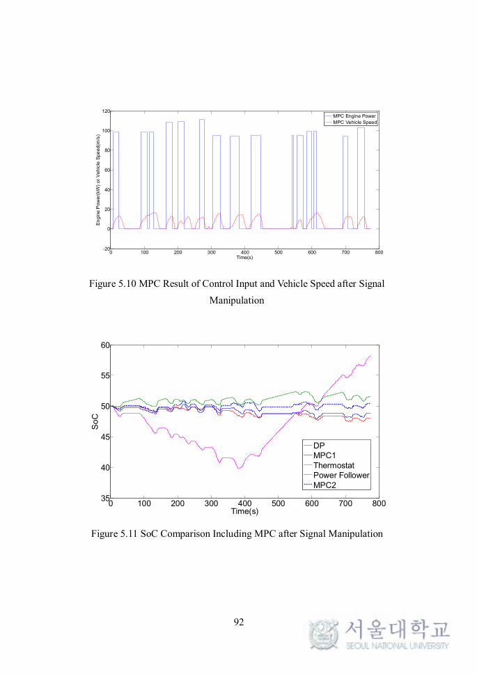
92

Figure 5.10 MPC Result of Control Input and Vehicle Speed after Signal

Manipulation

Figure 5.11 SoC Comparison Including MPC after Signal Manipulation

0 100 200 300 400 500 600 700 800-20

0

20

40

60

80

100

120

Time(s)

En

gin

e P

ow

er(

kW

) or

Vehic

le S

pe

ed(m

/s)

MPC Engine Power

MPC Vehicle Speed

0 100 200 300 400 500 600 700 80035

40

45

50

55

60

Time(s)

So

C

DPMPC1ThermostatPower FollowerMPC2

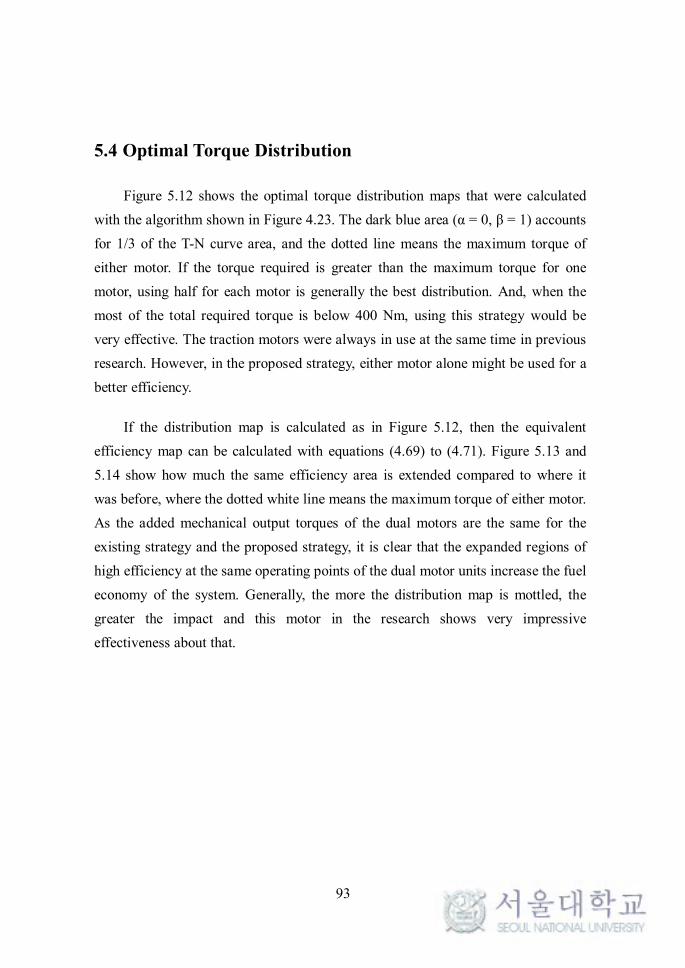
93

5.4 Optimal Torque Distribution

Figure 5.12 shows the optimal torque distribution maps that were calculated

with the algorithm shown in Figure 4.23. The dark blue area (α = 0, β = 1) accounts

for 1/3 of the T-N curve area, and the dotted line means the maximum torque of

either motor. If the torque required is greater than the maximum torque for one

motor, using half for each motor is generally the best distribution. And, when the

most of the total required torque is below 400 Nm, using this strategy would be

very effective. The traction motors were always in use at the same time in previous

research. However, in the proposed strategy, either motor alone might be used for a

better efficiency.

If the distribution map is calculated as in Figure 5.12, then the equivalent

efficiency map can be calculated with equations (4.69) to (4.71). Figure 5.13 and

5.14 show how much the same efficiency area is extended compared to where it

was before, where the dotted white line means the maximum torque of either motor.

As the added mechanical output torques of the dual motors are the same for the

existing strategy and the proposed strategy, it is clear that the expanded regions of

high efficiency at the same operating points of the dual motor units increase the fuel

economy of the system. Generally, the more the distribution map is mottled, the

greater the impact and this motor in the research shows very impressive

effectiveness about that.

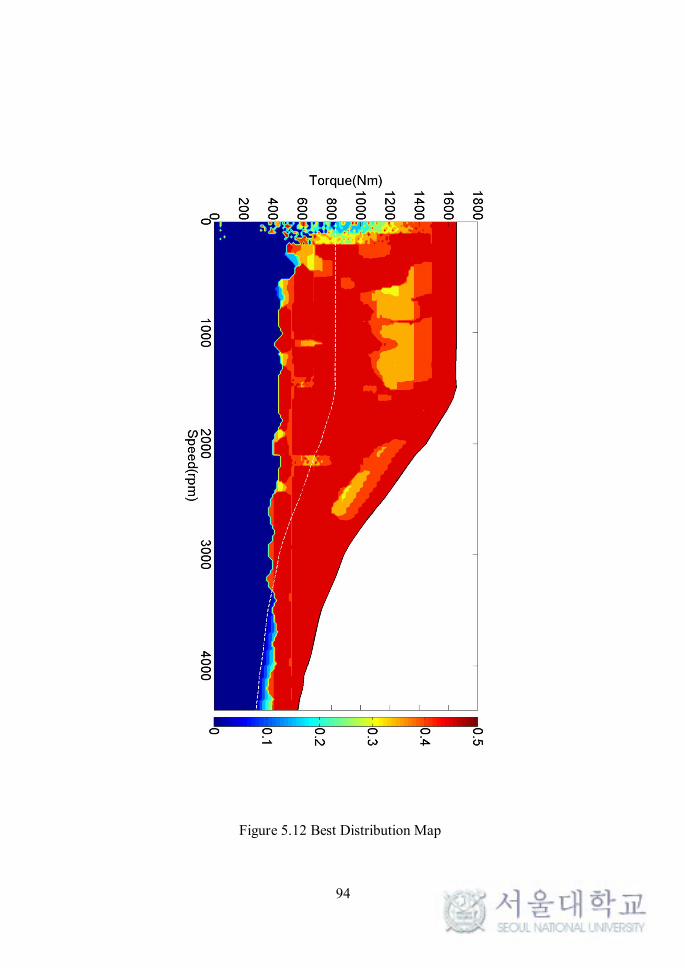
94

Figure 5.12 Best Distribution Map

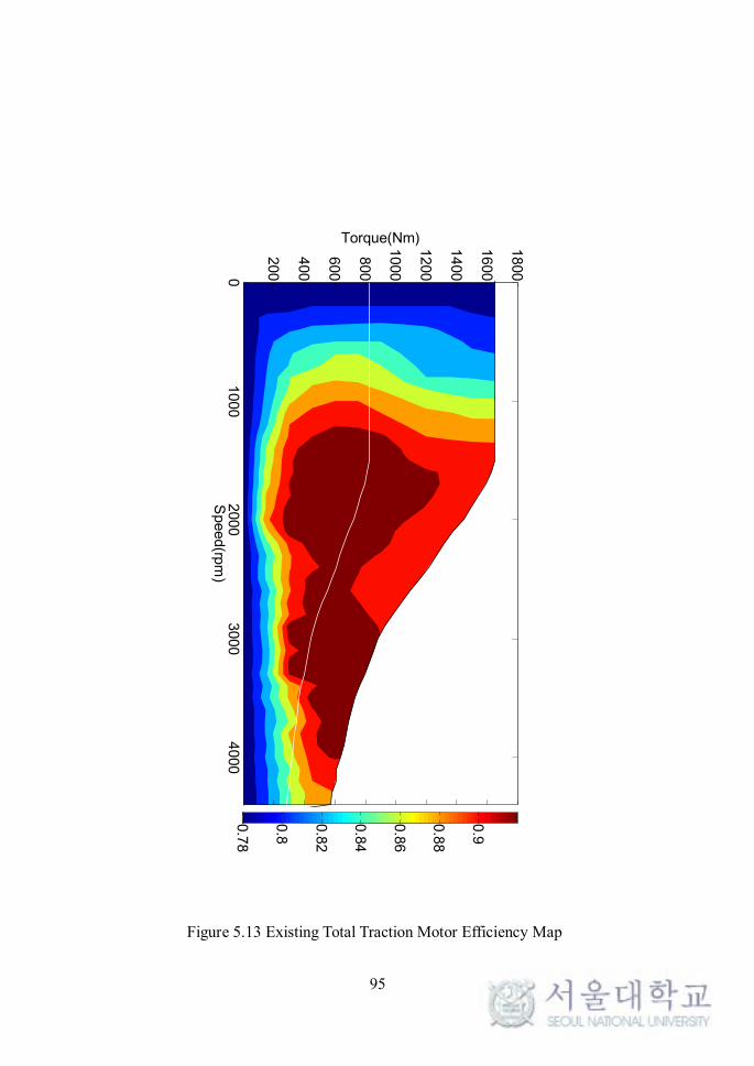
95

Figure 5.13 Existing Total Traction Motor Efficiency Map

Speed(rp

m)

Torque(Nm)

01000

2000

3000

4000

200

400

600

800

1000

1200

1400

1600

1800

0.7

8

0.8

0.8

2

0.8

4

0.8

6

0.8

8

0.9

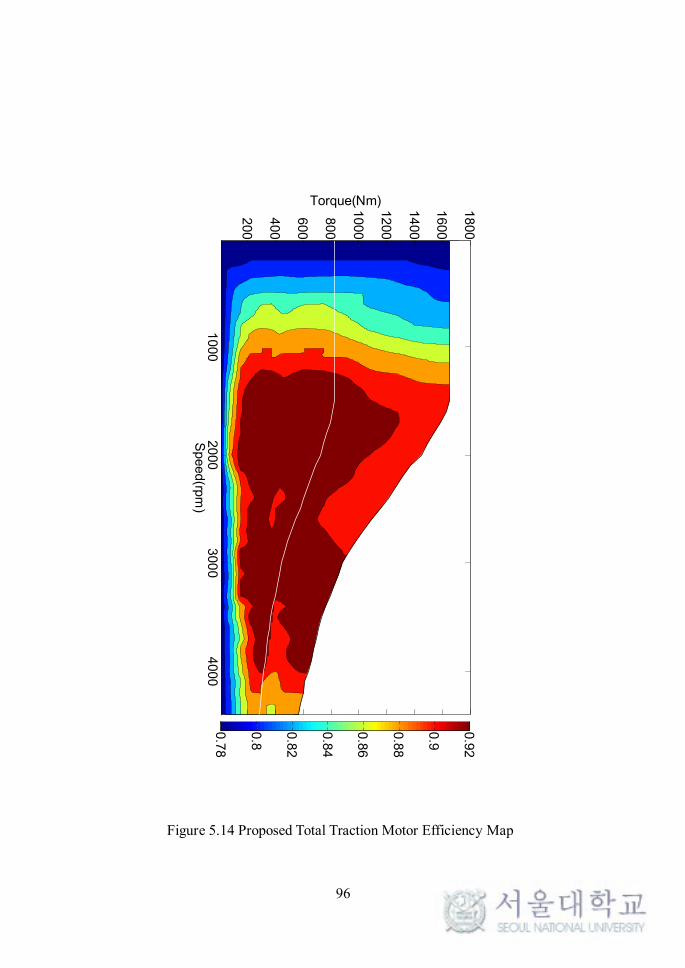
96

Figure 5.14 Proposed Total Traction Motor Efficiency Map

Speed(rp

m)

Torque(Nm)

1000

2000

300

04000

200

400

600

800

1000

1200

1400

1600

1800

0.7

8

0.8

0.8

2

0.8

4

0.8

6

0.8

8

0.9

0.9

2

97

Figure 5.15 shows a histogram comparison of the power difference according

to the total simulation time. The electrical motor power spent (or the re-generated

electrical motor power) considering the operating efficiency was calculated for

every time step for the cases of the half-and-half torque distribution and the

proposed distribution, and the more spent power (or the less re-generated power)

was calculated as in equations (5.1), (5.2) and (5.3):

1 1 2 22 / ( / / )half half opt opt opt optP P Ph h h´ - + : motoring (5.1)

1 1 2 22 ( )half half opt opt opt optP P Ph h h´ ´ - ´ + ´ : generating (5.2)

1 22 half opt optP P P´ = + , (5.3)

where halfP and halfh are the mechanical single-motor output power and the

single-motor efficiency with the half-and-half torque distribution, respectively, and

1optP , 1opth , 2optP and 2opth are the output power and the operating efficiency of

motor 1 and the output power and the operating efficiency of motor 2 with the

proposed distribution, respectively. Thus, the x-axis in Figure 5.15 is the more spent

electrical power at every time step (motoring), or the less re-generated electrical

power at every time step (re-generating), and the y-axis in Figure 5.15 gives the

number of occurrences throughout the simulation. For example, the condition

where 500 W (between 250 W and 750 W) more is spent (or less is re-generated)

occurs in approximately 12000 samples in the case shown in Figure 5.15

throughout the simulation run.

In Figure 5.15, the histogram bars exist mostly at the center or on the right side,

which proves that the proposed torque distribution is effective, as the half-and-half

torque distribution mostly spends the same or more power (or re-generates less

power). The number of occurrences below 100 was omitted, as the effects are minor.

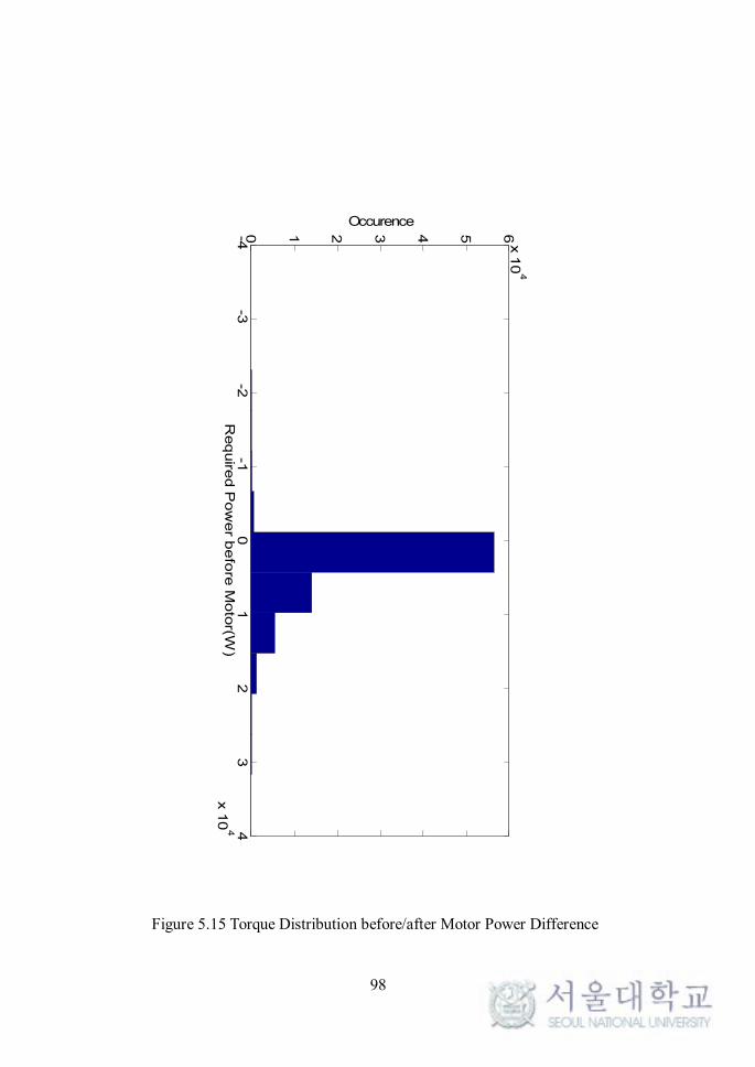
98

Figure 5.15 Torque Distribution before/after Motor Power Difference

-4-3

-2-1

01

23

4

x 1

04

0 1 2 3 4 5 6x 1

04

Require

d P

ow

er b

efo

re M

oto

r(W)

Occurence

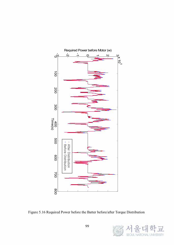
99

Figure 5.16 Required Power before the Batter before/after Torque Distribution

010

02

00

300

40

05

00

600

70

08

00

-3 -2 -1 0 1 2 3x 1

05

Tim

e(s

)

Required Power before Motor (w)

- A

fter D

istributio

n

- B

efo

re D

istrib

utio

n

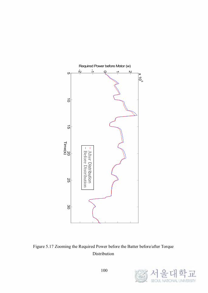
100

Figure 5.17 Zooming the Required Power before the Batter before/after Torque

Distribution

510

15

20

25

30

-2 -1 0 1 2

x 1

05

Tim

e(s

)

Required Power before Motor (w)

- A

fter D

istrib

utio

n

- B

efo

re D

istrib

utio

n

101

5.5 Mode Comparisons

Figure 5.18 to19 show the torque differences among the strategies. Map Motor

T1 is either motor using torque distribution and Map Motor T2 is the other of using

torque distribution. But, Half & Half 1 and 2 mean the motor with same torque.

These concepts are applied for all strategy from the engine to the battery energy

flow. Figure 5.18 shows the traction motor torque differences before/after torque

distribution. The light blue shadow means the regenerative mode which happen

when the torque in the traction motor negative and in Figure 5.19, the clear torque

difference can be seen.

Figure 5.20 and 21 show mode comparison of thermostat strategy, power

follower strategy, and the proposed strategy of semi MPC. The orange shadows

mean electric mode which is usually happen in the thermostat strategy but in the

case of power follower strategy and the proposed strategy, the important power

generation occur when the vehicle requires some power to overcome the road load.

Thus the vehicle becomes hybrid mode and is shadowed with light green color (it

can have some error when the prediction is not exact in MPC).

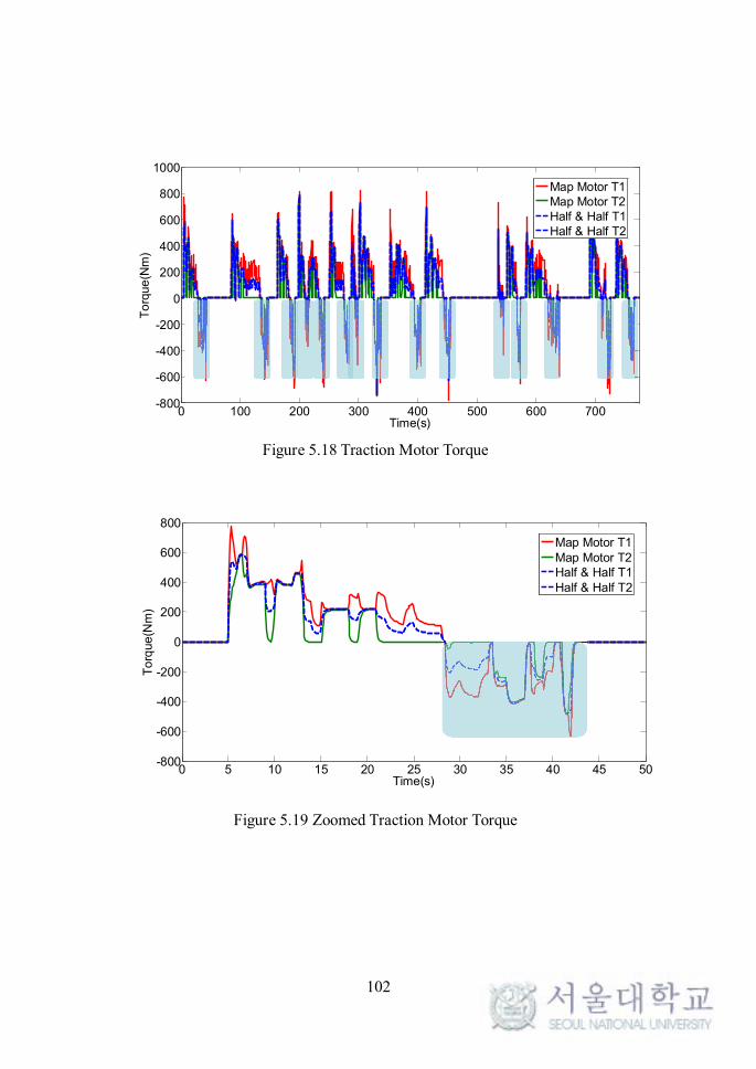
102

Figure 5.18 Traction Motor Torque

Figure 5.19 Zoomed Traction Motor Torque

0 100 200 300 400 500 600 700-800

-600

-400

-200

0

200

400

600

800

1000

Time(s)

To

rque

(Nm

)

Map Motor T1Map Motor T2Half & Half T1Half & Half T2

0 5 10 15 20 25 30 35 40 45 50-800

-600

-400

-200

0

200

400

600

800

Time(s)

To

rque

(Nm

)

Map Motor T1Map Motor T2Half & Half T1Half & Half T2

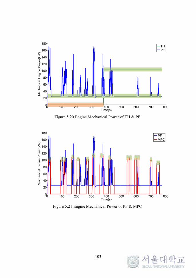
103

Figure 5.20 Engine Mechanical Power of TH & PF

Figure 5.21 Engine Mechanical Power of PF & MPC

0 100 200 300 400 500 600 700 8000

20

40

60

80

100

120

140

160

180

Time(s)

Mech

anic

al E

ngin

e P

ow

er(

kW

)

THPF

0 100 200 300 400 500 600 700 8000

20

40

60

80

100

120

140

160

180

Time(s)

Mech

anic

al E

ngin

e P

ow

er(

kW

)

PFMPC

104

5.6 Fuel Economy Comparison

Figure 5.22 shows the result of this research. All fuel economy improvement

was evaluated compared to DP1 result, where DP1 is the basic simulation result by

Dynamic Programming without signal manipulation. TH (thermostat strategy) or

PF (power follower strategy) results are less effective than DP1. And MPC1

(strategy which does not include signal manipulation technique and motor traction

torque distribution) also gives lower fuel economy than DP1. However, when the

signal manipulating techniques is applied, the fuel economy increase as much as

2.34 % better than DP1 and, when the torque distribution is added (MPC3), the

performance becomes 2.88 % better than that of DP1. However, the most efficiency

case is DP2 where the signal manipulation and torque distributions are used.

Basically, DP gives the ideal optimal calculation result in the backward

model. However, as the real-time simulation model requires a forward model, DP

result at the backward model cannot gives the best answer. Therefore, based on

semi MPC, signal manipulating and motor traction torque optimal distribution was

added and the results show very impressive fuel economy improvement.

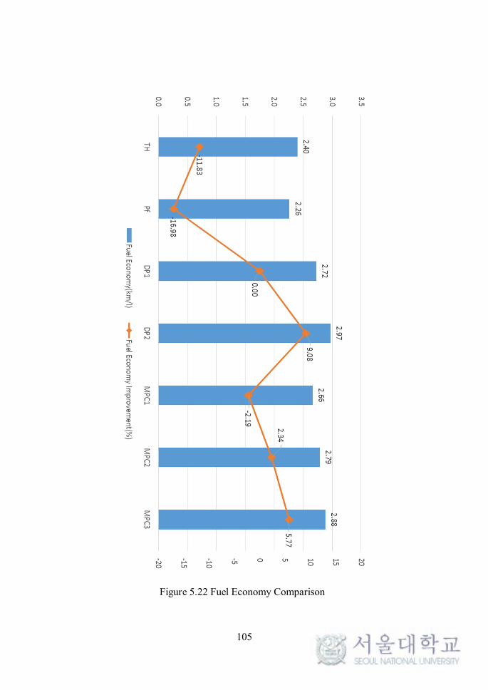
105

Figure 5.22 Fuel Economy Comparison

106

Chapter 6. Conclusions

In this study, a new strategy reducing the fuel consumption for series hybrid

electric intra-city bus is proposed. Intra-city bus is extremely well suited to hybrid

propulsion system because is capable of carrying the large payload required for the

battery and propulsion system. However, without an efficient energy management

strategy, the performance can be even worse than that of ICE vehicles. Thus, the

proposed strategy using NLP with speed prediction, signal manipulation and

traction motor torque distribution is developed, which is based on backward model

to the forward model transplanting.

The proposed strategy achieves the fuel economy of 2.88 km/l whereas DP

without motor torque distribution shows 2.72 km/l and DP with motor torque

distribution shows 2.97 km/l, where the DP calculation is reference given by the

pre-knowledge of all cycle information while the proposed strategy expects the

speed each section and does not know all speed information. Furthermore, the fuel

economy of the proposed strategy is much better than that of the conventional rule

based strategies, thermostat strategy of 2.40 km/l or power follower strategy of 2.26

km/l.

The advantages of the proposed strategy is that it solves the uncertain

standards of ‘When to generate or How much to generate?’ and shows the fast

calculation speed with exactness. It gives the full optimization solution from the

engine to the battery in SHEV which was not achieved before and all these are

demonstrated for the real bus test cycle with the online model. Thus, the fuel

economy is much improved with the real-time applicability and without a heavy

traffic jam or extraordinary accidents, this strategy would be very practical and

powerful.

107

All calculations are based on AMEsim and Simulink co-simulation and more

simplification of this strategy and using art-of-state NLP solver would be very

helpful for applying this strategy for the real SHEV intra-city buses.

108

Bibliography

[1] N. N. P. Wältermann, J. Weimer, and A. Bachmann, "A Testbed for the

Analysis of Performance and Efficiency of a Series Hybrid Drive Train,"

presented at the FISITA, 1998.

[2] J.-W. Xu and L. Zheng, "Simulation and Analysis of Series Hybrid Electric

Vehicle (SHEV) Based on ADVISOR," in Measuring Technology and

Mechatronics Automation (ICMTMA), 2010 International Conference on,

2010, pp. 354-357.

[3] E. R. C. Villante, "On energy performance of an electrically-driven city-car,"

presented at the EVS 26, L.A., 2012.

[4] H. Riebeek. (2010). Global Warming: Feature Articles. Available:

http://earthobservatory.nasa.gov/Features/GlobalWarming/page2.php

[5] D. Yihui, W. Zunya, S. Yafang, and Z. Jin, "The unprecedented freezing

disaster in January 2008 in southern China and its possible association with

the global warming," 象气 学报, vol. 22, 2008.

[6] D. S. Battisti and R. L. Naylor, "Historical warnings of future food insecurity

with unprecedented seasonal heat," Science, vol. 323, pp. 240-4, Jan 9 2009.

[7] Wikipedia, "Global warming."

[8] Doopedia, "global warming," in doopedia, ed. Korea: Doosan Corporation.

[9] J. Lu, G. A. Vecchi, and T. Reichler, "Expansion of the Hadley cell under

global warming," Geophysical Research Letters, vol. 34, 2007.

[10] A. Carnesale and W. Chameides, "America’s Climate Choices," NRC/NAS

USA Committee on America’s Climate Choices http://download. nap.

edu/cart/deliver. cgi, 2011.

[11] S. Solomon, Climate change 2007-the physical science basis: Working group I

contribution to the fourth assessment report of the IPCC vol. 4: Cambridge

University Press, 2007.

109

[12] I. P. O. C. Change, "Climate change 2007: the physical science basis," Agenda,

vol. 6, 2007.

[13] M. Koot, "Energy management for vehicular electric power systems," Ph.D.,

echnische Universiteit Eindhoven, 2007.

[14] A. Shen. (2011). Exxon Is Incredibly Bullish On The Future Of Hybrid

Vehicles. Available: http://www.businessinsider.com/exxon-is-incredibly-

bullish-on-the-future-of-hybrid-vehicles-2011-12

[15] R. Maly, "Spark ignition: its physics and effect on the internal combustion

engine," in Fuel Economy, ed: Springer, 1984, pp. 91-148.

[16] G. Abd-Alla, "Using exhaust gas recirculation in internal combustion engines:

a review," Energy Conversion and Management, vol. 43, pp. 1027-1042, 2002.

[17] M. Koot, "Energy management for vehicular electric power systems," PH.D.,

Technical University of Einthoven, 2006.

[18] L. N. Link. (2011). Exxon Is Incredibly Bullish On The Future Of Hybrid

Vehicles. Available: http://latestnewslink.com/2011/12/exxon-is-incredibly-

bullish-on-the-future-of-hybrid-vehicles/

[19] G. Q. Ao, J. A. Qiang, H. Zhong, L. Yang, and B. Zhuo, "Exploring the fuel

economy potential of ISG hybrid electric vehicles through dynamic

programming," International Journal of Automotive Technology, vol. 8, pp.

781-790, Dec 2007.

[20] A. Sciarretta and L. Guzzella, "Control of hybrid electric vehicles," Ieee

Control Systems Magazine, vol. 27, pp. 60-70, Apr 2007.

[21] P. Pisu and G. Rizzoni, "A comparative study of supervisory control strategies

for hybrid electric vehicles," Ieee Transactions on Control Systems Technology,

vol. 15, pp. 506-518, May 2007.

[22] M. Ehsani, Y. Gao, and A. Emadi, Modern electric, hybrid electric, and fuel

cell vehicles: fundamentals, theory, and design: CRC press, 2009.

[23] B. Bates, "Getting a Ford HEV on the road," Spectrum, IEEE, vol. 32, pp. 22-

25, 1995.

110

[24] W. Xiong, Y. Zhang, and C. Yin, "Optimal energy management for a series–

parallel hybrid electric bus," Energy Conversion and Management, vol. 50, pp.

1730-1738, 2009.

[25] F. R. Salmasi, "Control strategies for hybrid electric vehicles: Evolution,

classification, comparison, and future trends," Ieee Transactions on Vehicular

Technology, vol. 56, pp. 2393-2404, Sep 2007.

[26] K. Çağatay Bayindir, M. A. Gözüküçük, and A. Teke, "A comprehensive

overview of hybrid electric vehicle: Powertrain configurations, powertrain

control techniques and electronic control units," Energy Conversion and

Management, vol. 52, pp. 1305-1313, 2011.

[27] N. Jalil, N. A. Kheir, and M. Salman, "A rule-based energy management

strategy for a series hybrid vehicle," in American Control Conference, 1997.

Proceedings of the 1997, 1997, pp. 689-693.

[28] S. Farrall and R. Jones, "Energy management in an automotive electric/heat

engine hybrid powertrain using fuzzy decision making," in Intelligent Control,

1993., Proceedings of the 1993 IEEE International Symposium on, 1993, pp.

463-468.

[29] B. M. Baumann, G. Washington, B. C. Glenn, and G. Rizzoni, "Mechatronic

design and control of hybrid electric vehicles," Ieee-Asme Transactions on

Mechatronics, vol. 5, pp. 58-72, Mar 2000.

[30] J. Wu, C. H. Zhang, and N. X. Cui, "Fuzzy Energy Management Strategy for a

Hybrid Electric Vehicle Based on Driving Cycle Recognition," International

Journal of Automotive Technology, vol. 13, pp. 1159-1167, Dec 1 2012.

[31] J. M. Liu and H. E. Peng, "Modeling and Control of a Power-Split Hybrid

Vehicle," Ieee Transactions on Control Systems Technology, vol. 16, pp. 1242-

1251, Nov 2008.

[32] S. Yang, M. Li, H. Cui, Y. Cao, G. Wang, and Q. Lei, "Offline Optimization of

Plug-In Hybrid Electric Vehicle Energy Management Strategy Based on the

Dynamic Programming," in Intelligent Computing and Information Science,

ed: Springer, 2011, pp. 668-674.

111

[33] R. Johri and Z. Filipi, "Self-Learning Neural controller for Hybrid Power

Management using Neuro-Dynamic Programming," 2011.

[34] J. P. Gao, G. M. G. Zhu, E. G. Strangas, and F. C. Sun, "Equivalent fuel

consumption optimal control of a series hybrid electric vehicle," Proceedings

of the Institution of Mechanical Engineers Part D-Journal of Automobile

Engineering, vol. 223, pp. 1003-1018, Aug 2009.

[35] N. Kim, S. Cha, and H. Peng, "Optimal Control of Hybrid Electric Vehicles

Based on Pontryagin's Minimum Principle," Ieee Transactions on Control

Systems Technology, vol. 19, pp. 1279-1287, Sep 2011.

[36] G. Paganelli, S. Delprat, T.-M. Guerra, J. Rimaux, and J.-J. Santin,

"Equivalent consumption minimization strategy for parallel hybrid

powertrains," in Vehicular Technology Conference, 2002. VTC Spring 2002.

IEEE 55th, 2002, pp. 2076-2081.

[37] L. V. Pérez and E. A. Pilotta, "Optimal power split in a hybrid electric vehicle

using direct transcription of an optimal control problem," Mathematics and

Computers in Simulation, vol. 79, pp. 1959-1970, 2009.

[38] R. Johri, A. Salvi, and Z. Filipi, "Optimal energy management for a hybrid

vehicle using neuro-dynamic programming to consider transient engine

operation," in ASME 2011 Dynamic Systems and Control Conference and

Bath/ASME Symposium on Fluid Power and Motion Control, 2011, pp. 279-

286.

[39] R. Johri and Z. Filipi, "Low-cost pathway to ultra efficient city car: Series

hydraulic hybrid system with optimized supervisory control," 2010.

[40] Z. Filipi and Y. J. Kim, "Hydraulic Hybrid Propulsion for Heavy Vehicles:

Combining the Simulation and Engine-In-the-Loop Techniques to Maximize

the Fuel Economy and Emission Benefits," Oil & Gas Science and

Technology-Revue D Ifp Energies Nouvelles, vol. 65, pp. 155-178, Jan-Feb

2010.

[41] Y. J. Kim and Z. Filipi, "Simulation study of a series hydraulic hybrid

propulsion system for a light truck," Training, vol. 2008, pp. 12-10, 2007.

112

[42] S. Nabi, M. Balike, J. Allen, and K. Rzemien, "An overview of hardware-in-

the-loop testing systems at Visteon," SAE paper, vol. 5, 2004.

[43] M. Kim, D. Jeong, H. Kang, and K. Min, "Series-Type Hybrid Electric Bus

Fuel Economy Increase with Optimal Component Sizing and Real-Time

Control Strategy," Trans. Korean Soc. Mech. Eng. B, vol. 37, pp. 307-312,

2013.

[44] G. Ripaccioli, A. Bemporad, F. Assadian, C. Dextreit, S. Di Cairano, and I. V.

Kolmanovsky, "Hybrid modeling, identification, and predictive control: An

application to hybrid electric vehicle energy management," in Hybrid Systems:

Computation and Control, ed: Springer, 2009, pp. 321-335.

[45] J. T. Kessels, M. Koot, B. de Jager, P. P. van den Bosch, N. Aneke, and D. B.

Kok, "Energy management for the electric powernet in vehicles with a

conventional drivetrain," Control Systems Technology, IEEE Transactions on,

vol. 15, pp. 494-505, 2007.

[46] S. M. Lukic, S. G. Wirasingha, F. Rodriguez, J. Cao, and A. Emadi, "Power

management of an ultracapacitor/battery hybrid energy storage system in an

HEV," in Vehicle Power and Propulsion Conference, 2006. VPPC'06. IEEE,

2006, pp. 1-6.

[47] D. J. M. Kim, and K. Min, "Series Type Hybrid Bus Research of SILS

System," presented at the KSAE, 2010.

[48] D. J. M. Kim, and K. MIn, "Distribution Control Research on Series Hybrid

Electric Vehicle Bus," presented at the KSAE, 2011.

[49] J. Jeong, D. Lee, C. Shin, D. Jeong, K. Min, S. Cha, and Y.-i. Park,

"Comparison of the Fuel Economy of Series and Parallel Hybrid Bus System

Using Dynamic Programming," Transactions of KSAE, vol. 21, pp. 92-98,

2013.

[50] L. R. A. Chapman, "Adaptive Semi-Global Energy Management for a Series

Hybrid Performance Vehicle," presented at the EVS 26, L.A., 2012.

113

[51] M. D. Petersheim and S. N. Brennan, "Scaling of hybrid-electric vehicle

powertrain components for Hardware-in-the-loop simulation," Mechatronics,

vol. 19, pp. 1078-1090, 2009.

[52] D. J. Xuan, J. W. Kim, and Y. B. Kim, "Optimal operation strategy

development for fuel cell hybrid vehicle," Journal of Mechanical Science and

Technology, vol. 25, pp. 183-192, Jan 2011.

[53] W. W. Pulkrabek, Engineering fundamentals of the internal combustion engine

vol. 2: Pearson Prentice Hall New Jersey, 2004.

[54] P. K. Devan and N. V. Mahalakshmi, "Performance, emission and combustion

characteristics of poon oil and its diesel blends in a DI diesel engine," Fuel,

vol. 88, pp. 861-867, May 2009.

[55] C.-C. Lin, Z. Filipi, Y. Wang, L. Louca, H. Peng, D. Assanis, and J. Stein,

Integrated, feed-forward hybrid electric vehicle simulation in SIMULINK and

its use for power management studies: SAE, 2001.

[56] W. Wang, X. Zeng, and Q. Wang, "Develop hybrid transit buses for chinese

cities," Training, vol. 2013, pp. 11-04, 2003.

[57] K. M. D. Jung, Y. Cho, and Y. Lim, "Study on the optimization of generation

system in a Series HEV Bus," presented at the KSME, 2010.

[58] J. H. Mathews and K. D. Fink, Numerical methods using MATLAB vol. 31:

Prentice hall Upper Saddle River, NJ, 1999.

[59] M. E. Al-Mualla, C. N. Canagarajah, and D. R. Bull, "Simplex minimization

for single- and multiple-reference motion estimation," Ieee Transactions on

Circuits and Systems for Video Technology, vol. 11, pp. 1209-1220, Dec 2001.

[60] W. G. Yim, K. O. An, J. H. Seo, M. J. Kim, and H. K. Jung, "Shape

Optimization for Interior Permanent Magnet Motor based on Hybrid

Algorithm," Journal of Electrical Engineering & Technology, vol. 7, pp. 64-68,

Jan 2012.

[61] J. Farnsworth, T. Bono, H. Mizuno, and Y. Tano, "Development of a Vehicle

Model for FCHV Control and Functional Specification Development within a

Software-in-the-Loop Simulation Environment," Safety, vol. 2013, pp. 04-08.

114

[62] K. O. An, C. H. Im, and H. K. Jung, "Magnetoencephalography source

localization using improved simplex method," Inverse Problems in Science

and Engineering, vol. 16, pp. 499-510, 2008.

[63] W.-G. Yim, K.-O. An, J.-H. Seo, D.-K. Woo, and H.-K. Jung, "A study of the

notch shape optimization for a BLAC motor by using the Response Surface

Method and Improved Simplex Method," in 2010 International Conference on

Electrical Machines and Systems, 2010, pp. 1268-1272.

[64] Z. Filipi and Y. Kim, "Hydraulic hybrid propulsion for heavy vehicles:

Combining the simulation and engine-in-the-loop techniques to maximize the

fuel economy and emission benefits," Oil & Gas Science and Technology–

Revue de l’Institut Français du Pétrole, vol. 65, pp. 155-178, 2009.

[65] Y. J. Kim and Z. Filipi, "Simulation study of a series hydraulic hybrid

propulsion system for a light truck," SAE paper, pp. 01-4151, 2007.

[66] Y. J. Kim and Z. Filipi, "Series hydraulic hybrid propulsion for a light truck–

optimizing the thermostatic power management," SAE Transactions, Journal

of Engines, vol. 116, pp. 24-0080, 2007.

[67] G. Fontaras, P. Pistikopoulos, and Z. Samaras, "Experimental evaluation of

hybrid vehicle fuel economy and pollutant emissions over real-world

simulation driving cycles," Atmospheric Environment, vol. 42, pp. 4023-4035,

Jun 2008.

[68] J. Gao, F. Sun, H. He, G. G. Zhu, and E. G. Strangas, "A comparative study of

supervisory control strategies for a series hybrid electric vehicle," in Power

and Energy Engineering Conference, 2009. APPEEC 2009. Asia-Pacific, 2009,

pp. 1-7.

[69] J. Gao, G. M. G. Zhu, E. Strangas, and F. Sun, "Equivalent fuel consumption

optimal control of a series hybrid electric vehicle," Proceedings of the

Institution of Mechanical Engineers, Part D: Journal of Automobile

Engineering, vol. 223, pp. 1003-1018, 2009.

115

[70] R. Johri, A. Salvi, and Z. Filipi, "Optimal Energy Management for a Hybrid

Vehicle Using Neuro-Dynamic Programming to Consider Transient Engine

Operation," 2011.

[71] D. E. Kirk, Optimal control theory: an introduction: Courier Dover

Publications, 2012.

[72] J. M. Maciejowski, Predictive control: with constraints: Pearson education,

2002.

[73] D. P. Bertsekas, D. P. Bertsekas, D. P. Bertsekas, and D. P. Bertsekas, Dynamic

programming and optimal control vol. 1: Athena Scientific Belmont, MA,

1995.

[74] N. Kim, "Energy management strategy for hybrid electric vehicles based on

pontryagin’s minimum principle," Seoul National University, 2009.

[75] M. Koot, J. T. Kessels, B. de Jager, W. Heemels, P. Van den Bosch, and M.

Steinbuch, "Energy management strategies for vehicular electric power

systems," Vehicular Technology, IEEE Transactions on, vol. 54, pp. 771-782,

2005.

[76] M. Back, M. Simons, F. Kirschaum, and V. Krebs, "Predictive control of

drivetrains," in World Congress, 2002, pp. 1506-1506.

[77] F. Yan, J. Wang, and K. Huang, "Hybrid electric vehicle model predictive

control torque-split strategy incorporating engine transient characteristics,"

Vehicular Technology, IEEE Transactions on, vol. 61, pp. 2458-2467, 2012.

[78] Wikipedia. Model Predictive Control. Available:

http://en.wikipedia.org/wiki/Model_predictive_control

[79] M. Cannon. Model Predictive Control. Available:

http://www.eng.ox.ac.uk/~conmrc/mpc/index.html

[80] G. Ao, J. Qiang, H. Zhong, L. Yang, and B. Zhuo, "Exploring the fuel

economy potential of ISG hybrid electric vehicles through dynamic

programming," Int. J. Automotive Technology, vol. 8, pp. 781-790, 2007.

[81] J. T. Betts, Practical methods for optimal control and estimation using

nonlinear programming vol. 19: Siam, 2010.

116

[82] D. Xuan, J. Kim, and Y. Kim, "Optimal operation strategy development for

fuel cell hybrid vehicle," Journal of Mechanical Science and Technology, vol.

25, pp. 183-192, 2011.

[83] E. D. Tate and S. P. Boyd, "Finding ultimate limits of performance for hybrid

electric vehicles," SAE transactions, vol. 109, pp. 2437-2448, 2000.

[84] L. Pérez and G. García, "State constrained optimal control applied to

supervisory control in HEVs," Oil & Gas Science and Technology–Revue de

l’Institut Français du Pétrole, vol. 65, pp. 191-201, 2010.

[85] M. Kim, D. Jeong, and K. Min, "Serie Type Hybrid Bus Research of SILS

System," 2010, pp. 2929-2934.

117

초 록

시리즈 이 리드차 연구에 가장 큰 이슈 나는 ‘엔진

이 닛 부 모 지 어떻게 에 지를 달 것인가?’

이다. 이를 달 해 많 이 들이 시 었지만, 존 연구들

그 용 이 모 거나, 용 자체가 어 거나, 는 용

배경이 요구 었다. 게다가 고 어 운 략일

이상 인 모델 반 여 모든 보를 아는 것 가 고 를

풀어 에, 그 실 이 떨어 다. 라 간단 략들이 실

어 리 이 에 사용 어 다. 본 연구에 는 이러 략들

약 극복 는 연 향상 에 지분배 략이 시 었다.

가능 속도에 해 계획법 높 과 른

계산속도는 실 인 안 고 다. 해당 략 계획법 및

속도 개 반 백워드 모델에 계획법 사용 여

소 연료량 발 지 값 추출 여 에 지 분배를 는

것 골자 다. 여 에 신 처리 및 견인모 닛에 토크분배도

부가함 써 이 리드 차량 연 를 이룰 있었다. 결국

구조 간단함 에 다소 도외시 직 이 리드 차량 특히

버스에 해 고 효 이루는 독특 방법 시 여, 병 이나

직별 이 리드 차량이 보 지 못 효 인 방법

연 를 이룩 있었다. 안 방법 직 이 리드

차량 배 질 감에도 여 것 다.

키워드: 구동 발 , 에 지 리, 어, 워 발 컨트 ,

실시간 시스 , 시리즈 이 리드 버스

번: 2010-30182