Embed Size (px)
Citation preview

저 시-비 리- 경 지 2.0 한민
는 아래 조건 르는 경 에 한하여 게
l 저 물 복제, 포, 전송, 전시, 공연 송할 수 습니다.
다 과 같 조건 라야 합니다:
l 하는, 저 물 나 포 경 , 저 물에 적 된 허락조건 명확하게 나타내어야 합니다.
l 저 터 허가를 면 러한 조건들 적 되지 않습니다.
저 에 른 리는 내 에 하여 향 지 않습니다.
것 허락규약(Legal Code) 해하 쉽게 약한 것 니다.
Disclaimer
저 시. 하는 원저 를 시하여야 합니다.
비 리. 하는 저 물 리 목적 할 수 없습니다.
경 지. 하는 저 물 개 , 형 또는 가공할 수 없습니다.
Ph.D. Dissertation
Spatial Sound Reproduction byWave Field Synthesis with Frontal
Linear Loudspeaker Arrays
전방선형라우드스피커배열을이용한
음장합성재생기법
August 2012
Graduate School of Seoul National University
School of Electrical Engineering and Computer Science
Hyunjoo Chung

Spatial Sound Reproduction byWave Field Synthesis with Frontal Linear
Loudspeaker Arrays
전방선형라우드스피커배열을이용한
음장합성재생기법
지도교수남상욱
이논문을공학박사학위논문으로제출함
2012년 4월
서울대학교대학원
전기·컴퓨터공학부정현주
정현주의박사학위논문을인준함
2012년 6월
위 원 장 (인)
부위원장 (인)
위 원 (인)
위 원 (인)
위 원 (인)


Abstract
This dissertation describes a sound reproduction method that uses linear
front loudspeaker arrays. In the horizontal plane of the listening area, sound
images are reproduced separately by two processes on the basis of wave
field synthesis (WFS). First, the front sound images are synthesized as plane
waves. Second, the lateral or rear sound images are rendered as focused
sources and reflected by sidewalls. To widen the listening area, a linear
loudspeaker array system with steered directivity is proposed, providing the
convenience of installation with a display device. To reproduce 3-D acous-
tic images, the horizontal plane of the loudspeakers should be extended in
the vertical direction using additional loudspeakers. Double-layered loud-
speaker arrays are proposed for the reproduction of sound images on the
vertical plane in front of a listener. Rendering based on WFS is used to lo-
calize virtual sources in both azimuth and elevation. First, a 2-D wave field
is synthesized by a virtual loudspeaker array, and then each column, consist-
ing of an upper and lower loudspeaker pair, generates virtual loudspeakers
by vertical amplitude panning using calculated elevation vectors. Compu-
tational simulations were conducted to evaluate the proposed method. Sub-
jective listening tests comparing the proposed method to 3-D vector base
amplitude panning were conducted to evaluate the frontal localization qual-
i

ity of this system.
Keywords : Sound reproduction, loudspeaker array, steered loudspeaker
array, wave field synthesis, focused source, WFS vertical panning
Student Number : 2007-30245
ii
Table of Contents
I. Introduction . . . . . . . . . . . . . . . . . . . . . . . . . . . 1
1.1 Motivation for This Study . . . . . . . . . . . . . . . . . . . 1
1.2 Contributions and Outline of the Dissertation . . . . . . . . 4
II. Basic Principles of Wave Field Synthesis . . . . . . . . . . . . 5
2.1 Wave Field Synthesis . . . . . . . . . . . . . . . . . . . . . 5
2.1.1 Huygens’ Principle . . . . . . . . . . . . . . . . . . 5
2.1.2 The Kirchhoff–Helmholtz Integral . . . . . . . . . . 6
2.1.3 Rayleigh’s Representation Theorem . . . . . . . . . 13
2.1.4 Adaptation for Practical Application . . . . . . . . . 15
2.2 Adaptation of Loudspeaker Directivity Model . . . . . . . . 21
2.2.1 Modeling of Loudspeaker as a Circular Piston Ra-
diator . . . . . . . . . . . . . . . . . . . . . . . . . 22
2.2.2 Calculation of the Driving Function . . . . . . . . . 26
2.3 Optimization of Loudspeaker Arrays . . . . . . . . . . . . . 31
2.3.1 Loudspeaker Arrays with Steered Directivity . . . . 31
2.3.2 Additional Sound Field Processing . . . . . . . . . . 35
III. Spatial Sound Reproduction by WFS . . . . . . . . . . . . . 37
3.1 Sound Reproduction on a Horizontal Plane . . . . . . . . . . 38
3.1.1 Front Channels Rendered by Plane Waves . . . . . . 41
iii

3.1.2 Virtual Surround Channels by Focused Sources . . . 44
3.2 Sound Reproduction on a Vertical Plane . . . . . . . . . . . 47
3.2.1 3-D Vector Base Amplitude Panning . . . . . . . . . 48
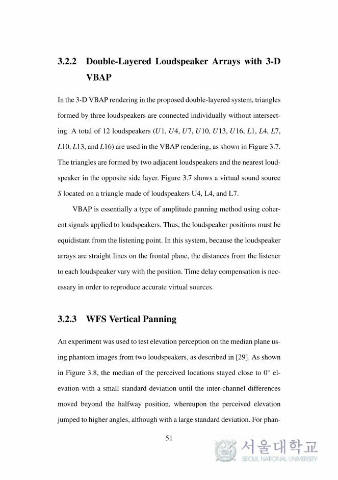
3.2.2 Double-Layered Loudspeaker Arrays with 3-D VBAP 51
3.2.3 WFS Vertical Panning . . . . . . . . . . . . . . . . 51
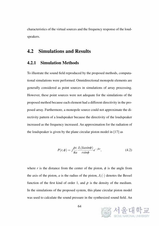
IV. Implementation and Simulations . . . . . . . . . . . . . . . . 61
4.1 Specifications of Implemented System . . . . . . . . . . . . 61
4.1.1 Pre-Equalization Filter . . . . . . . . . . . . . . . . 63
4.2 Simulations and Results . . . . . . . . . . . . . . . . . . . . 64
4.2.1 Simulation Methods . . . . . . . . . . . . . . . . . 64
4.2.2 Simulations of Steered Array . . . . . . . . . . . . . 65
4.2.3 Simulations of Focused Source Reflections . . . . . 66
4.2.4 Simulations of Double-Layered Arrays . . . . . . . 76
4.3 Subjective Assessment . . . . . . . . . . . . . . . . . . . . 93
4.3.1 Horizontal Localization . . . . . . . . . . . . . . . 93
4.3.2 Vertical Localization . . . . . . . . . . . . . . . . . 102
V. Conclusion . . . . . . . . . . . . . . . . . . . . . . . . . . . . 117
Bibliography . . . . . . . . . . . . . . . . . . . . . . . . . . . . . . 119
iv
List of Figures
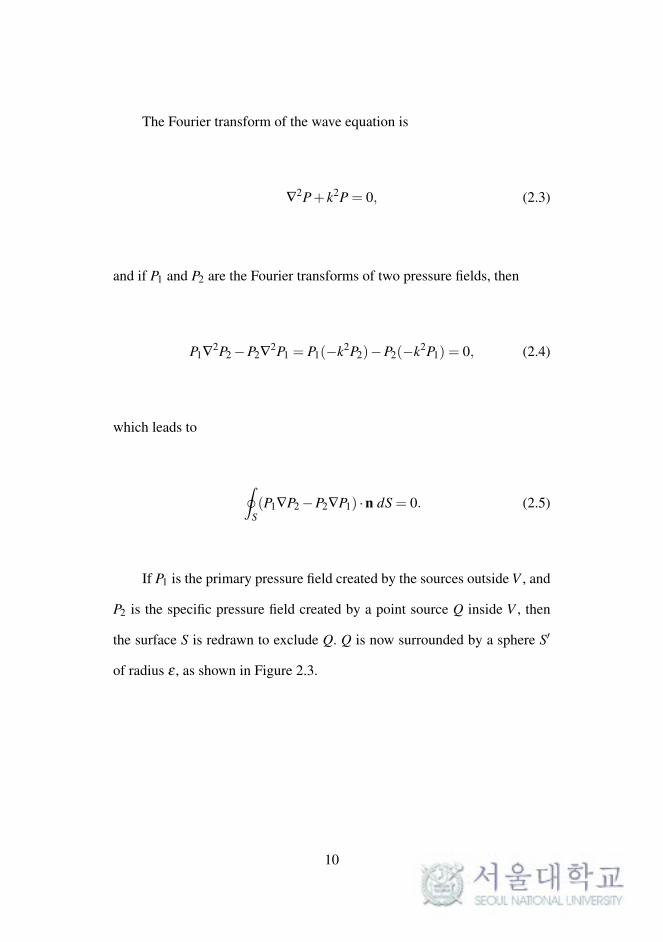
Fig. 2.1. Huygens’ principle and the role of loudspeakers as sec-
ondary sources . . . . . . . . . . . . . . . . . . . . . . 7
Fig. 2.2. Definition of the parameters used for the Kirchhoff–
Helmholtz integral. . . . . . . . . . . . . . . . . . . . . 9
Fig. 2.3. Modified region of integration. . . . . . . . . . . . . . . 11
Fig. 2.4. Geometry for Rayleigh’s representation theorem. . . . . 14
Fig. 2.5. Vertical and horizontal views of simulated sound field. . 16
Fig. 2.6. Geometry for the calculation of the driving functions. . . 20
Fig. 2.7. Directivity of a circular piston radiator. . . . . . . . . . 23
Fig. 2.8. Geometry of a baffled circular piston . . . . . . . . . . 24
Fig. 2.9. Loudspeaker arrays for WFS to widen the listening area. 33
Fig. 2.10. Uniformly spaced linear array with directive loudspeak-
ers steered according to the arc-shaped array. . . . . . . 34
Fig. 3.1. Layout and coordinates of sound reproduction on a hor-
izontal plane. . . . . . . . . . . . . . . . . . . . . . . . 39
Fig. 3.2. Example of signal flow diagrams in the proposed method. 40
Fig. 3.3. Geometry for calculating driving functions for N-loudspeaker
array. . . . . . . . . . . . . . . . . . . . . . . . . . . . 42
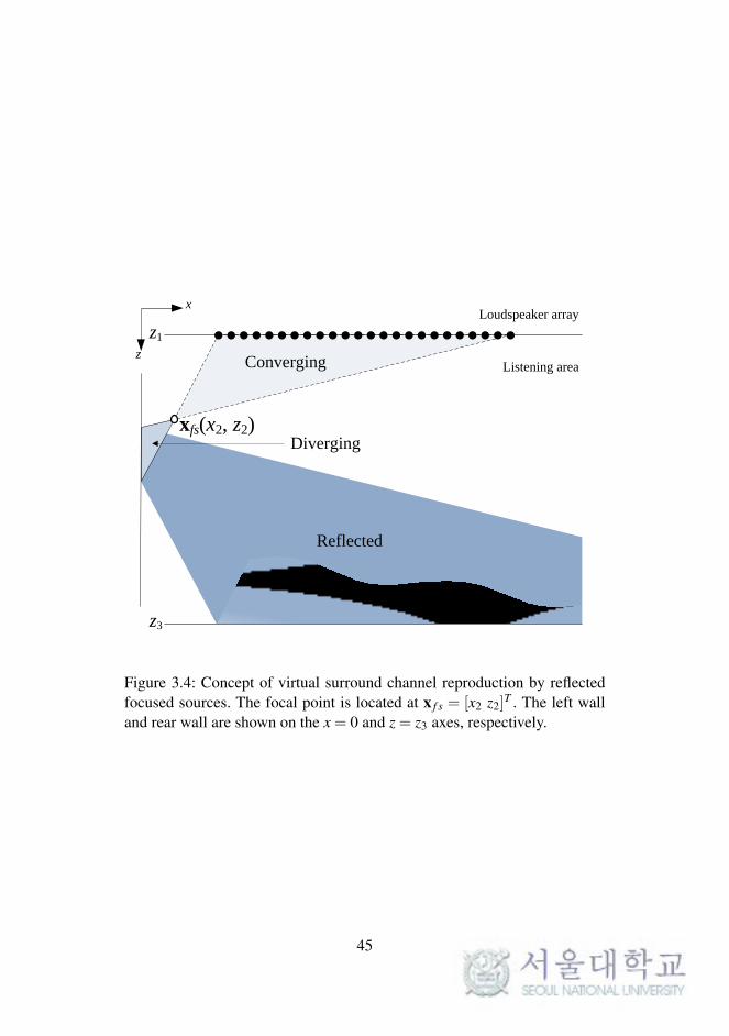
Fig. 3.4. Concept of virtual surround channel reproduction by re-
flected focused sources. . . . . . . . . . . . . . . . . . 45
v
Fig. 3.5. Layout and coordinates of sound reproduction on a ver-
tical plane. . . . . . . . . . . . . . . . . . . . . . . . . 49
Fig. 3.6. Example of 3-D VBAP . . . . . . . . . . . . . . . . . . 49
Fig. 3.7. Implementation of 3-D VBAP rendering . . . . . . . . . 52
Fig. 3.8. Localization test of elevation perception in median plane
between 0 and 45. . . . . . . . . . . . . . . . . . . . 54
Fig. 3.9. Localization test of elevation perception in median plane
between 0 and 60. . . . . . . . . . . . . . . . . . . . 55
Fig. 3.10. Localization test of elevation perception in median plane
between 0 and 90. . . . . . . . . . . . . . . . . . . . 56
Fig. 3.11. Example of 2-D WFS expanded to three dimensions by
VBAP. . . . . . . . . . . . . . . . . . . . . . . . . . . 57
Fig. 3.12. Proposed 3-D expansion model of WFS system. . . . . 59
Fig. 4.1. Average frequency response (on-axis) of loudspeaker
units used in the proposed array. . . . . . . . . . . . . . 62
Fig. 4.2. Difference in SIL between steered directivity array and
normal array. θp = 30, f = 250 Hz or 500 Hz . . . . . 67
Fig. 4.3. Difference in SIL between steered directivity array and
normal array. θp = 30, f = 1 kHz or 2 kHz . . . . . . . 68
Fig. 4.4. Difference in SIL between steered directivity array and
normal array. θp = 0, f = 250 Hz or 500 Hz . . . . . . 69
Fig. 4.5. Difference in SIL between steered directivity array and
normal array. θp = 0, f = 1 kHz or 2 kHz . . . . . . . 70
vi
Fig. 4.6. Sound pressure and SIL distributions of focused source.
f = 250 Hz . . . . . . . . . . . . . . . . . . . . . . . . 72
Fig. 4.7. Sound pressure and SIL distributions of focused source.
f = 500 Hz . . . . . . . . . . . . . . . . . . . . . . . . 73
Fig. 4.8. Sound pressure and SIL distributions of focused source.
f = 1 kHz . . . . . . . . . . . . . . . . . . . . . . . . . 74
Fig. 4.9. Sound pressure and SIL distributions of focused source.
f = 2 kHz . . . . . . . . . . . . . . . . . . . . . . . . . 75
Fig. 4.10. Comparison of 3-D sound pressure field. f = 500 Hz,
ys = 0. . . . . . . . . . . . . . . . . . . . . . . . . . . 78
Fig. 4.11. Comparison of 3-D sound pressure field. f = 1 kHz,
ys = 0. . . . . . . . . . . . . . . . . . . . . . . . . . . 79
Fig. 4.12. Comparison of 3-D sound pressure field. f = 2 kHz,
ys = 0. . . . . . . . . . . . . . . . . . . . . . . . . . . 80
Fig. 4.13. Comparison of 3-D sound pressure field. f = 500 Hz,
ys = 0.5. . . . . . . . . . . . . . . . . . . . . . . . . . 81
Fig. 4.14. Comparison of 3-D sound pressure field. f = 1 kHz,
ys = 0.5. . . . . . . . . . . . . . . . . . . . . . . . . . 82
Fig. 4.15. Comparison of 3-D sound pressure field. f = 2 kHz,
ys = 0.5. . . . . . . . . . . . . . . . . . . . . . . . . . 83
Fig. 4.16. Comparison of 3-D sound pressure field. f = 500 Hz,
ys = 1.0. . . . . . . . . . . . . . . . . . . . . . . . . . 84
vii
Fig. 4.17. Comparison of 3-D sound pressure field. f = 1 kHz,
ys = 1.0. . . . . . . . . . . . . . . . . . . . . . . . . . 85
Fig. 4.18. Comparison of 3-D sound pressure field. f = 2 kHz,
ys = 1.0. . . . . . . . . . . . . . . . . . . . . . . . . . 86
Fig. 4.19. Comparison of 3-D sound pressure field. f = 500 Hz,
ys = 1.5. . . . . . . . . . . . . . . . . . . . . . . . . . 87
Fig. 4.20. Comparison of 3-D sound pressure field. f = 1 kHz,
ys = 1.5. . . . . . . . . . . . . . . . . . . . . . . . . . 88
Fig. 4.21. Comparison of 3-D sound pressure field. f = 2 kHz,
ys = 1.5. . . . . . . . . . . . . . . . . . . . . . . . . . 89
Fig. 4.22. Comparison of 3-D sound pressure field. f = 500 Hz,
ys = 2.0. . . . . . . . . . . . . . . . . . . . . . . . . . 90
Fig. 4.23. Comparison of 3-D sound pressure field. f = 1 kHz,
ys = 2.0. . . . . . . . . . . . . . . . . . . . . . . . . . 91
Fig. 4.24. Comparison of 3-D sound pressure field. f = 2 kHz,
ys = 2.0. . . . . . . . . . . . . . . . . . . . . . . . . . 92
Fig. 4.25. Layout of localization test on horizontal plane. . . . . . 94
Fig. 4.26. Localization test results for distance. (pink noise) . . . . 97
Fig. 4.27. Localization test results for azimuth. (pink noise) . . . . 98
Fig. 4.28. Localization test results for distance. (musical signal) . . 99
Fig. 4.29. Localization test results for azimuth. (musical signal) . . 100
Fig. 4.30. Side view of loudspeaker arrays and listener. . . . . . . 101
viii
Fig. 4.31. Screen capture of the GUI program used for the vertical
localization test. . . . . . . . . . . . . . . . . . . . . . 104
Fig. 4.32. Results of loudspeaker perception tests. . . . . . . . . . 106
Fig. 4.33. Total results of mean values in Test 1. . . . . . . . . . . 108
Fig. 4.34. Total results of mean values in Test 2. . . . . . . . . . . 108
Fig. 4.35. Result (1) of vertical localization test using pink noise. . 110
Fig. 4.36. Result (2) of vertical localization test using pink noise. . 111
Fig. 4.37. Result (3) of vertical localization test using pink noise. . 111
Fig. 4.38. Result (4) of vertical localization test using pink noise. . 112
Fig. 4.39. Result (5) of vertical localization test using pink noise. . 112
Fig. 4.40. Result (1) of vertical localization test using mixed signal. 113
Fig. 4.41. Result (2) of vertical localization test using mixed signal. 113
Fig. 4.42. Result (3) of vertical localization test using mixed signal. 114
Fig. 4.43. Result (4) of vertical localization test using mixed signal. 114
Fig. 4.44. Result (5) of vertical localization test using mixed signal. 115
ix

x
Chapter 1
Introduction
1.1 Motivation for This Study
Although diverse sound reproduction techniques have been introduced over
the years to enrich the sound quality, surround sound systems for home the-
ater applications have not changed considerably and still use discrete loud-
speaker channels from devices ranging from a simple two-channel stereo
to a 10.2-channel surround system. Because the content in such systems is
generally created using panning methods [1], the standard layout configu-
ration defined in the ITU-R Recommendation BS. 775-1 [2] is widely used
for reproduction systems such as the DVD and Blu-ray disc.
On the basis of research on spatial audio, some audio reproduction sys-
tems beyond the 5.1-channel system have been commercially introduced
and discussed for cinema applications, home theater applications, and broad-
casting formats. In particular, after the success of 3-D movie content and
during the standardization of ultrahigh-definition television (UHDTV), ef-
forts dedicated to spatial audio have become more active, e.g., IOSONO [3]
1
as a cinema application and a 22.2-channel layout by NHK [4].
Although the content rendered for the 22.2-channel layout realizes out-
standing localization and plays realistic sounds, this method requires accu-
rate installation of 24 loudspeakers around the entire listening area in order
to provide the desired reproduction because the sound images are rendered
by panning. Considering that the broadcasting format should be designed
for home applications, the accurate installation of 24 loudspeakers becomes
economically and practically questionable.
In addition to panning techniques, wave field synthesis (WFS) is an-
other possible candidate for home applications. This technique is based on
acoustic holography [5] and physically reconstructs wave propagation from
the primary source by using a multiple-loudspeaker array [6]. Spatial sound
reproduction by WFS has major advantages over a discrete surround sound
system. In a WFS system, the range of the optimal listening area, in which
accurate localization of notional sound sources is ensured, is considerably
wider than the sweet spot of conventional surround systems [7, 8]. More-
over, notional sources in the listening area in front of the loudspeaker arrays,
which are called focused sources [9], can be synthesized.
Nonetheless, WFS has the same economical and practical problems be-
cause it requires the installation of dozens to even hundreds of loudspeak-
ers [10]. Because WFS is based on the Kirchhoff–Helmholtz integral for
a closed surface, ideal WFS requires many loudspeakers surrounding the
entire listening area.
2

A virtual surround technology, also known as a digital sound projec-
tor, based on beam forming by a loudspeaker array has been introduced
for convenient installation [11]. This technology reproduces a rear-channel
sound image by reflecting a strong sound beam, created by a sound bar,
from walls; hence, this technology offers easier installation than a conven-
tional 5.1-channel system. However, the digital sound projector still has a
narrow sweet spot resulting from the discrete surround sound.
In many sound reproduction systems with a display device, such as cin-
ema, UHDTV, or conventional home theater systems, most sound images are
generally localized in front of listeners along with the visual objects. Fur-
thermore, lateral sound localization by the human auditory system is less
accurate than front and rear localization; this is known as “localization blur”
[12]. Accordingly, frontal sound localization becomes more important than
that in the rear channels in terms of the localization probability and human
auditory characteristics. A WFS-based sound reproduction system that as-
signs a relatively high priority to frontal localization is introduced in this
dissertation. The proposed system uses a linear array that can be mounted
on a display device. The system synthesizes frontal sound images as both
plane waves and spherical waves by using WFS, whereas the side and rear
sound images are obtained by using focused sources and are reflected by the
sidewalls [13]. Further, a sound rendering method using a double-layered
loudspeaker array is proposed for the reproduction of 3-D acoustic images
in front of the listening area. To provide a relatively wide listening area lim-
3
ited by the length of the array, steering methods for loudspeaker directivity
are also introduced.
1.2 Contributions and Outline of the Disserta-
tion
This dissertation is organized as follows. Chapter 2 describes the basic prin-
ciples of WFS. The traditional WFS operator using simple monopole point
sources is improved by including the directivity characteristics of each loud-
speaker. Monopole sources were replaced by a circular piston radiator model.
Using this proposed model, an arc-directional linear loudspeaker array is
introduced to optimize the reproduced listening area. Chapter 3 presents
the proposed reproduction methods based on WFS rendering to reproduce
virtual sound sources by using plane waves and focused sources in a hori-
zontal or vertical plane. When a front-only loudspeaker array is used, a vir-
tual surround channel method using focused sound sources is proposed to
compensate for the absence of a lateral or rear channel in the loudspeakers.
Furthermore, a WFS vertical panning method is proposed to expand sound
images on the horizontal plane to three dimensions. Chapter 4 explains the
implementation of the proposed system. Furthermore, results obtained by
computational simulations and subjective localization assessments of the
proposed system are also discussed. Finally, concluding remarks are sum-
marized in Chapter 5.
4
Chapter 2
Basic Principles of Wave Field
Synthesis
This chapter explains WFS as a spatial sound field reproduction technique.
Basic principles such as the Kirchhoff–Helmholtz integral and Rayleigh’s
representation theorem are used to reproduce the sound field by a loud-
speaker array. Consequently, the driving function of each loudspeaker in
the array is also calculated. Moreover, a circular piston radiator model is
adapted to the elements of the loudspeaker array. The proposed circular pis-
ton radiator model can exhibit the directivity pattern of actual loudspeaker
units.
2.1 Wave Field Synthesis
2.1.1 Huygens’ Principle
Because an array of point sources is used, the acoustic field may be treated
by taking the superposition of the spherical waves emanating from each
5
source. As a result, we can accept the plausibility of a useful and historically
important development known as Huygens’ principle, which may be stated
as follows:
Each point on a wavefront (called the primary) may be regarded
as a source of secondary hemispherical waves that propagate in
the forward direction and whose envelope at any time consti-
tutes a new primary wavefront.
Huygens formulated this principle in 1690 on the basis of physical intu-
ition. Subsequently, he and others used it to provide a framework to explain
a wide variety of propagation phenomena [14]
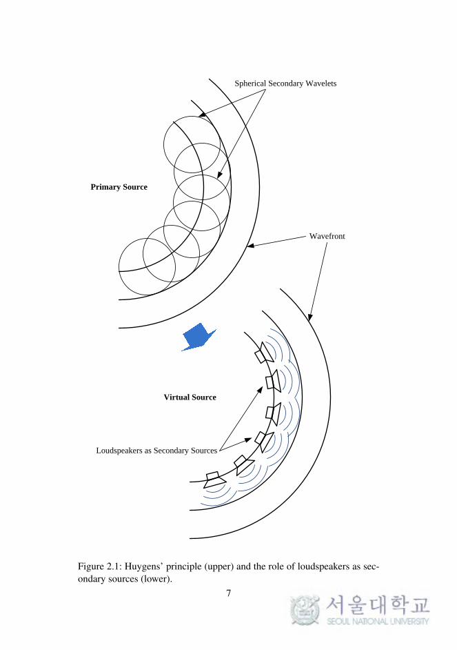
For a wave emitted by a point source Ps with a frequency f , all the
points on the wavefront at any time t can be taken as point sources for the
production of spherical secondary wavelets of the same frequency. Then, at
the next instant, this wavefront is the envelope of the secondary wavelets, as
shown in Figure 2.1. All the secondary wavelets are coherent, which means,
in this context, that they all have the same frequency and phase [15].
2.1.2 The Kirchhoff–Helmholtz Integral
WFS is based on Huygens’ principle, which was quantified by Kirchhoff.
His theorem states that at any listening point L within a source-free vol-
ume V , the sound pressure can be calculated if both the sound pressure and
the component of the particle velocity can be known on a surface S en-
closing V by considering a distribution of monopole and dipole sources on
6
Primary Source
Spherical Secondary Wavelets
Wavefront
Virtual Source
Loudspeakers as Secondary Sources
Figure 2.1: Huygens’ principle (upper) and the role of loudspeakers as sec-ondary sources (lower).
7
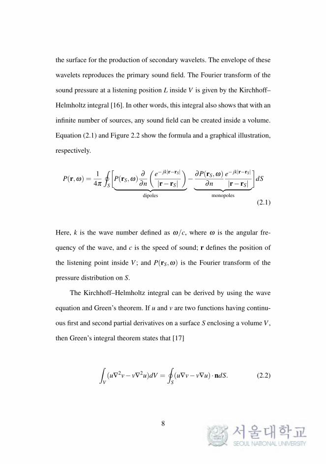
the surface for the production of secondary wavelets. The envelope of these
wavelets reproduces the primary sound field. The Fourier transform of the
sound pressure at a listening position L inside V is given by the Kirchhoff–
Helmholtz integral [16]. In other words, this integral also shows that with an
infinite number of sources, any sound field can be created inside a volume.
Equation (2.1) and Figure 2.2 show the formula and a graphical illustration,
respectively.
P(r,ω) =1
4π
∮S
[P(rS,ω)
∂
∂n
(e− jk|r−rS|
|r− rS|
)︸ ︷︷ ︸
dipoles
− ∂P(rS,ω)
∂ne− jk|r−rS|
|r− rS|︸ ︷︷ ︸monopoles
]dS
(2.1)
Here, k is the wave number defined as ω/c, where ω is the angular fre-
quency of the wave, and c is the speed of sound; r defines the position of
the listening point inside V ; and P(rS,ω) is the Fourier transform of the
pressure distribution on S.
The Kirchhoff–Helmholtz integral can be derived by using the wave
equation and Green’s theorem. If u and v are two functions having continu-
ous first and second partial derivatives on a surface S enclosing a volume V ,
then Green’s integral theorem states that [17]
∫V(u∇
2v− v∇2u)dV =
∮S(u∇v− v∇u) ·ndS. (2.2)
8
Primary Source
V S
L
Sr rn
Figure 2.2: Definition of the parameters used for the Kirchhoff–Helmholtzintegral.
9
The Fourier transform of the wave equation is
∇2P+ k2P = 0, (2.3)
and if P1 and P2 are the Fourier transforms of two pressure fields, then
P1∇2P2 −P2∇
2P1 = P1(−k2P2)−P2(−k2P1) = 0, (2.4)
which leads to
∮S(P1∇P2 −P2∇P1) ·n dS = 0. (2.5)
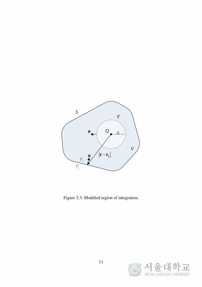
If P1 is the primary pressure field created by the sources outside V , and
P2 is the specific pressure field created by a point source Q inside V , then
the surface S is redrawn to exclude Q. Q is now surrounded by a sphere S′
of radius ε , as shown in Figure 2.3.
10
V
S
Sr rn
n Q
S
2P
1P
Figure 2.3: Modified region of integration.
11
Note that P2 = A e− jkd
d with d = |r− rS|; then
∮S+S′
[e− jkd
d∂P1
∂n−P1
∂
∂n
(e− jkd
d
)]dS = 0
∮S′
[e− jkd
d∂P1
∂n−P1
∂
∂n
(e− jkd
d
)]dS′
=−∮
S
[e− jkd
d∂P1
∂n−P1
∂
∂n
(e− jkd
d
)]dS.
(2.6)
On S′, d = ε and dS′ = ε2dΩ, where Ω is the solid angle, and ∂
∂n = ∂
∂d .
Equation (2.6) becomes
∫ 4π
0
[e− jkε
ε
∂P1
∂d+P1
e− jkε
ε
(jk+
1ε
)]ε
2dΩ
=−∮
S
[e− jkd
d∂P1
∂n−P1
∂
∂n
(e− jkd
d
)]dS.
(2.7)
Taking ε → 0,
∫ 4π
0P1(Q)dΩ = 4πP1(Q) =−
∮S
[e− jkd
d∂P1
∂n−P1
∂
∂n
(e− jkd
d
)]dS.
(2.8)
Then, the Kirchhoff–Helmholtz integral (2.1) is obtained. It can also be writ-
12
ten as
P(r,ω) =1
4π
∮S
(jωρ0Vn(rS,ω)
e− jkd
d+P(rS,ω)
1+ jkdd
cosϕe− jkd
d
)dS,
(2.9)
where ρ0 is the air density, and Vn is the particle velocity in the direction of
n.
2.1.3 Rayleigh’s Representation Theorem
The Kirchhoff–Helmholtz integral shows that by setting the correct pressure
distribution P(rS,ω) and its gradient on a surface S, a sound field in the
volume enclosed within this surface can be created.
To implement a realizable system, the surface S must be reduced to a
plane z = z1 separating the source area from the listening area, as shown in
Figure 2.4. The Kirchhoff–Helmholtz integral (2.1) can be simplified into
the Rayleigh I integral for monopoles (2.10) and the Rayleigh II integral for
dipoles (2.11).
P(r,ω) = ρ0cjk
2π
∫ ∫S
(Vn(rS,ω)
e− jk|r−rS|
|r− rS|
)dS (2.10)
P(r,ω) =jk
2π
∫ ∫S
(P(rS,ω)
1+ jk|r− rS|jk|r− rS|
cosϕe− jk|r−rS|
|r− rS|
)dS (2.11)
13
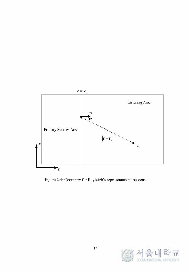
L
Sr r
n
z
x
1z z
Primary Sources Area
Listening Area
Figure 2.4: Geometry for Rayleigh’s representation theorem.
14

Here ρ0 denotes the air density; c is the speed of sound in air; k is the wave
number; and Vn is the particle velocity in the direction of n.
2.1.4 Adaptation for Practical Application
2.1.4.1 Discretization
So far, we have considered a continuous distribution of sources on the sur-
face. In reality, the sources in the plane are loudspeakers, so the distribution
is discrete.
This leads to the discrete forms of Rayleigh’s integrals [18].
For Rayleigh I,
P(r,ω) =jωρ0
2π
∞∑n=1
Vn(rn,ω)e− jk|r−rn|
|r− rn|∆x∆y, (2.12)
and for Rayleigh II,
P(r,ω) =1
2π
∞∑n=1
Pn(rn,ω)1+ jk|r− rn|
|r− rn|cosϕ
e− jk|r−rn|
|r− rn|∆x∆y. (2.13)
The calculations below are based on the Rayleigh I integral.
15
Simulated wavfronts
Notional source far
away
Simulated wavfronts
Notional source far
away
length
wid
thh
eig
ht
z
x
z
y
Figure 2.5: Vertical and horizontal views of simulated sound field.
16
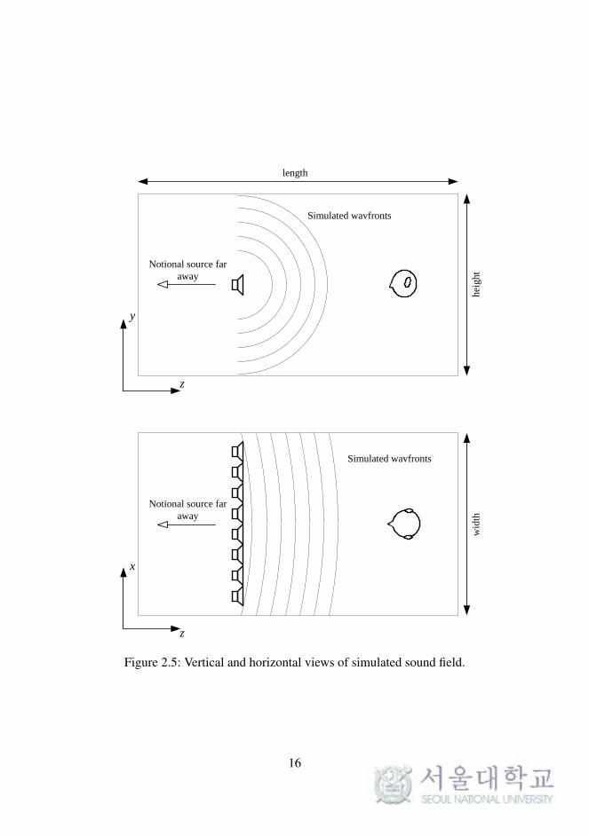
2.1.4.2 Reduction to a line
For practical reasons, the surface is reduced to a line. The listener is assumed
to be in the plane y = y1. Reducing the planar array to a line does not affect
the shape of the wavefronts in the xz-plane, as shown in Figure 2.5. Only
the shape of the wavefront in the horizontal ear plane actually affects the
perception of sound.
The discrete form of the Rayleigh I integral (2.12) can be transformed
into
P(r,ω) =jωρ0
2π
∞∑n=1
(Vn(rn,ω)
e− jk|r−rn|
|r− rn|
)∆x. (2.14)
2.1.4.3 Calculation of the driving functions
The sound pressure P(rn,ω) is linked to the particle velocity Vn(rn,ω) through
the specific acoustic impedance Z [17] as follows:
Z(r,ω) =P(r,ω)
V (r,ω). (2.15)
For a spherical wave, the specific acoustic impedance is given by
Z(r,ω) =ρc
1+ 1jkr
(r = 0), (2.16)
17
where r is the distance to the point source.
For a pulsating sphere of average radius a and angular frequency ω , the
radial component of the velocity of the fluid in contact with the sphere is cal-
culated using the specific acoustic impedance for a spherical wave evaluated
at r = a.
Vn(rn,ω) =P(rn,ω)
ρ0c
(1+
1jka
)(2.17)
For a discrete distribution of pulsating spheres of average radius a, (2.14)
becomes
P(r,ω) =
(jk
2π+
12πa
) ∞∑n=1
[P(rn,ω)
e− jk|r−rn|
|r− rn|
]∆x. (2.18)
In a practical application, the sources are loudspeakers with a cer-
tain directivity instead of ideal pulsating spheres. The pressure has to be
weighted by a factor that depends on the directivity G(ϕn,ω). The pressure
at each loudspeaker must be weighted by a factor An(rn,ω) to account for
the fact that the sound source is no longer omnidirectional.
Hence, the discrete form of the one-dimensional Rayleigh I integral
18
(2.14) can be written as follows.
P(r,ω) =∞∑
n=1
[An(rn,ω)P(rn,ω)G(ϕn,ω)
e− jk|r−rn|
|r− rn|
]∆x (2.19)
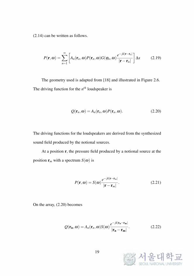
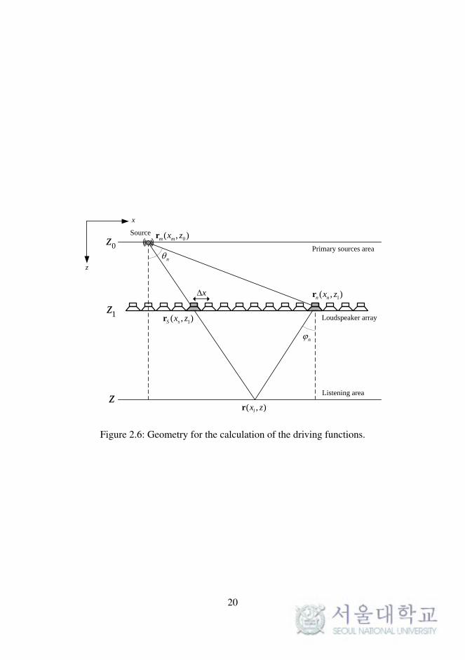
The geometry used is adapted from [18] and illustrated in Figure 2.6.
The driving function for the nth loudspeaker is
Q(rn,ω) = An(rn,ω)P(rn,ω). (2.20)
The driving functions for the loudspeakers are derived from the synthesized
sound field produced by the notional sources.
At a position r, the pressure field produced by a notional source at the
position rm with a spectrum S(ω) is
P(r,ω) = S(ω)e− jk|r−rm|
|r− rm|. (2.21)
On the array, (2.20) becomes
Q(rn,ω) = An(rn,ω)S(ω)e− jk|rn−rm|
|rn − rm|. (2.22)
19
z
x
Primary sources area
Source
1z
0z
Loudspeaker array
Listening area
0( , )mm x zr
n
1( , )sS x zr
x1( , )nn x zr
n
z( , )lx zr
Figure 2.6: Geometry for the calculation of the driving functions.
20
Given the pressure field of the notional source at a listening position r, (2.19)
becomes
S(ω)e− jk|r−rm|
|r− rm|=
N∑n=1
[Q(rn,ω)G(ϕn,ω)
e− jk|r−rn|
|r− rn|
]∆x, (2.23)
or, replacing Q with (2.19) and canceling out S(ω),
e− jk|r−rm|
|r− rm|=
N∑n=1
[An(rn,ω)
e− jk|rn−rm|
|rn − rm|G(ϕn,ω)
e− jk|r−rn|
|r− rn|
]∆x. (2.24)
The driving function can be calculated using a mathematical method called
the stationary-phase approximation [6]. After substantial mathematical ma-
nipulations, we find that the driving function can be described by
Q(rn,ω) = S(ω)cos(θn)
Gn(θn,ω)
√jk
2π
√|z− z1||z− z0|
e− jk|rn−rm|√|rn − rm|
. (2.25)
2.2 Adaptation of Loudspeaker Directivity Model
In the previous section, the driving functions for WFS were calculated on the
basis of Rayleigh’s representation theorem. During the calculation, the dis-
cretized Rayleigh integrals prescribe the use of planar arrays of monopoles
as loudspeakers. However, radiated sound pressure from the actual loud-
speaker unit is distinguished from that of the monopole source. Most loud-
21
speakers radiate the sound preferably in a certain direction except at very
low frequencies [19]. As described in (2.25), a linear array of loudspeak-
ers with arbitrary directivity characteristics can be operated to synthesize
the desired wave field by correcting the weighting functions of the WFS
operators, as described in [18]. However, the elements of the array were
still assumed to be monopole sources during integration. In this section, the
loudspeaker radiation pattern is modeled as a circular piston radiator in an
infinite baffle. Then the sound pressure from the loudspeaker array is calcu-
lated by a linear array of the modeled circular piston radiators.
2.2.1 Modeling of Loudspeaker as a Circular Piston
Radiator
A monopole source cannot approximate the directivity pattern of a loud-
speaker ideally. The loudspeaker’s radiation pattern is omnidirectional only
at low frequencies, whereas it becomes more directional as the reproduced
frequency increases. The directivity also depends on the loudspeaker’s di-
ameter. A circular piston can be a good approximation of a loudspeaker
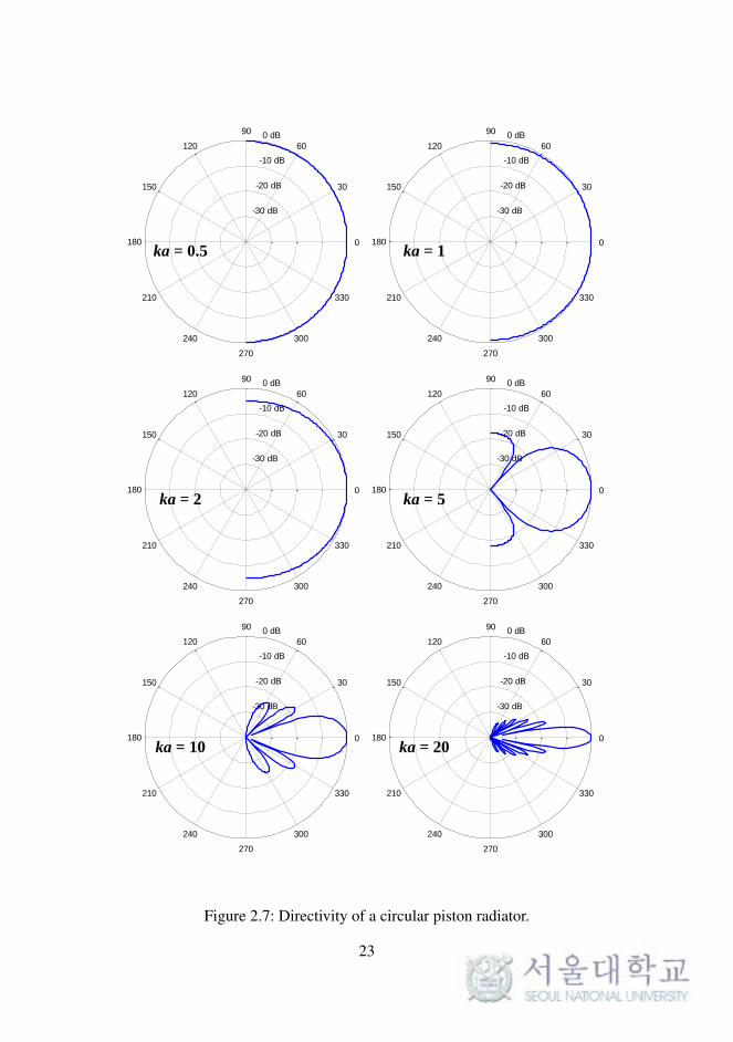
[20]. Figure 2.7 shows the directional radiation pattern of the circular piston
radiator in an infinite baffle. The graphs in the figure are labeled according
to the value of ka, which is the product of the piston radius a and the given
wave number k.
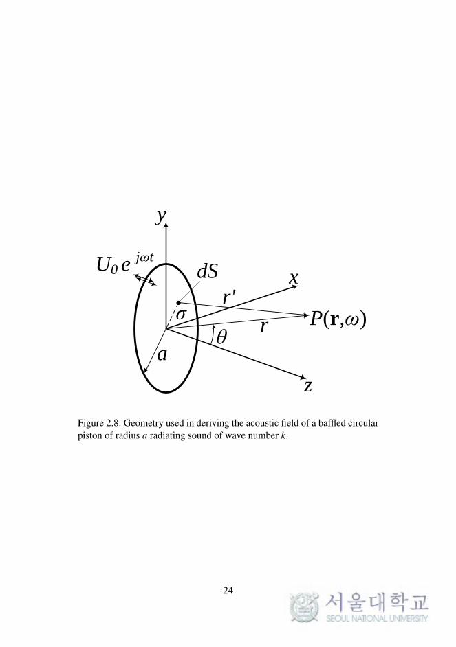
The pressure at any field point can be obtained by dividing the surface
of the piston into infinitesimal elements as shown in Figure 2.8, each of
22
-30 dB
-20 dB
-10 dB
0 dB
30
210
60
240
90
270
120
300
150
330
180 0
-30 dB
-20 dB
-10 dB
0 dB
30
210
60
240
90
270
120
300
150
330
180 0
-30 dB
-20 dB
-10 dB
0 dB
30
210
60
240
90
270
120
300
150
330
180 0
-30 dB
-20 dB
-10 dB
0 dB
30
210
60
240
90
270
120
300
150
330
180 0
-30 dB
-20 dB
-10 dB
0 dB
30
210
60
240
90
270
120
300
150
330
180 0
-30 dB
-20 dB
-10 dB
0 dB
30
210
60
240
90
270
120
300
150
330
180 0
ka = 0.5
ka = 2
ka = 10
ka = 1
ka = 5
ka = 20
Figure 2.7: Directivity of a circular piston radiator.
23
x
z
y
θr P(r,ω)
a
U0 e jωt
σ
dS
r'
Figure 2.8: Geometry used in deriving the acoustic field of a baffled circularpiston of radius a radiating sound of wave number k.
24

which acts as a baffled simple source of strength dQ = U0dS. Because the
pressure generated by one of these sources is given by
P = ρ0cQ/λ r, (2.26)
the total pressure is
P(r,ω) = jρ0cU0
λ
∫S
e− jkr′
r′dS, (2.27)
where the surface integral is taken over the region σ 5 a. By taking the
approximation of the far field such that the field point r is sufficiently distant
compared with the piston radius a, (2.27) can be derived as
P(r,ω) =j2
ρ0cU0ar
ka[
2J1(kasinθ)
kasinθ
]e− jkr. (2.28)
The entire angular dependence term in the brackets is simplified as
H(θ) =
∣∣∣∣2J1(v)v
∣∣∣∣ v = kasinθ . (2.29)
25
If N circular piston radiator elements are arranged linearly at intervals of ∆x,
the sound pressure produced by the nth piston radiator is given by
Pn(r,ω) =j2
ρ0cUna
|r− rn|ka[
2J1(kasinθn)
kasinθn
]e− jk|r−rn|
=j2
ρ0a2ω ·UnH(θn,ω)
e− jk|r−rn|
|r− rn|.
(2.30)
Similar to the case of the Rayleigh I integral (2.14), by using (2.21) and
(2.30), the sound pressure of circular piston radiator array can be derived as
P(r,ω) =j2
ρ0a2ω
N∑n=1
[Un
e− jk|rn−rm|
|rn − rm|H(θn,ω)
e− jk|r−rn|
|r− rn|
]. (2.31)
2.2.2 Calculation of the Driving Function
With the geometry shown in Figure 2.6, the driving function is defined as
Q(r,ω) =UnS(ω)e− jk|rm−rn|
|rm − rn|. (2.32)
26
To find the weighting factor Un, (2.31) and (2.32) should be the same; thus,
e− jk|r−rm|
|r− rm|=
N∑n=1
[UnH(ϕn,ω)
|rn − rm||r− rn|e− jk(|rn−rm|+|r−rn|)
](2.33)
by the stationary-phase approximation [21], assuming
I =e− jk|r−rm|
|r− rm|
α(xn) =k(|rn − rm|+ |r− rn|)
f (xn) =UnH(ϕn,ω)
|rn − rm||r− rn|.
(2.34)
Then, (2.33) becomes
I =1
∆x
N∑n=1
f (xn)e− jα(xn)∆x (2.35)
by the stationary-phase approximation because α(xn) is a rapidly varying
function that has a minimum at xsp, such that α ′(xs) = 0. Therefore, it is
27
assumed that f (xn) = f (xs). Hence,
I =f (xs)
∆x
√2π
jα ′′s
e− jα(xs). (2.36)
In the stationary-phase approximation, most of the energy radiated by the
array to a specific listening position is produced by the loudspeaker that is
on a direct path from the source to the receiver. Mathematical manipulations
yield the value of the stationary point as follows:
xsp = xm +|xl − xm||z1 − z0|
|z− z0|. (2.37)
Then,
α′′(xs) = k
[(|xl + xm||z− z0|
)2
+1
]−3/2|z− z0|
|z− z1||z1 − z0|, (2.38)
|r− rs|= |z− z1|
√(xl − xm
z− z0
)2
+1
|rs − rm|= |z1 − z0|
√(xl − xm
z− z0
)2
+1.
(2.39)
28
Thus, f (xs) can be calculated as follows:
f (xs) =UsH(ϕs,ω)
|rs − rm||r− rs|=
UsH(ϕs,ω)
|z− z1||z1 − z0|[(
|xl−xm||z−z0|
)2+1] . (2.40)
At the point of the stationary phase, ϕs is equivalent to θs, and
|rs − rm|+ |r− rs|= |r− rm|.
Using these results, I becomes
I =UsH(θs,ω)
|z− z1||z1 − z0|[(
|xl−xm||z−z0|
)2+1]√2π
j
×
[(xl + xm
z− z0
)2
+1
] 34√
|z− z1||z1 − z0|k|z− z0|
1∆x
(2.41)
Using the definition of I in (2.35),
1|r− rm|
=UsH(θs,ω)√
|z− z1||z1 − z0||z− z0|
√2π
jk
[(|xl + xm||z− z0|
)2
+1
]− 14 1
∆x.
(2.42)
29
After some manipulations, the weighting function is obtained:
Us =
√jk
2π
1H(θs,ω)
√|z− z1||z− z0|
z1 − z0√|rs − rm|
1∆x
. (2.43)
Because every loudspeaker can become a stationary point by varying the lis-
tening position, the last equation can be generalized for the nth loudspeaker:
Un =
√jk
2π
1H(θn,ω)
√|z− z1||z− z0|
z1 − z0√|rn − rm|
1∆x
. (2.44)
Therefore, the driving function is obtained as
Q(rn,ω) = S(ω)cosθn
H(θn,ω)
√jk
2π
√|z− z1||z− z0|
e− jk|rn−rm|√|rn − rm|
1∆x
. (2.45)
By comparison with the previous driving function (2.25), this can be re-
garded as a specialized form of the driving function for secondary monopole
sources,
Gn(θn,ω) = H(θn,ω) ·∆x. (2.46)
30
2.3 Optimization of Loudspeaker Arrays
Propagating wavefronts are closely related to the perceptual directions of
sound sources in the listening area. By using loudspeaker arrays, the WFS
method can synthesize wavefronts by using plane waves that have the same
propagation direction at any point in the listening area. Because of this fea-
ture of WFS, the optimum listening area obtained by using WFS becomes
wider than the sweet spot obtained by discrete surround sounds. However,
the area of the propagating wavefronts synthesized by WFS is restricted by
the arrangement of the arrays and the virtual sound source. Therefore, the
total length of the loudspeaker array becomes a decisive factor in the width
of the optimal listening area when a front array is used.
2.3.1 Loudspeaker Arrays with Steered Directivity
In a practical array with limited length, it is impossible to increase the de-
fined optimal listening area physically. Nonetheless, an effectively wider lis-
tening area can be obtained by decreasing the localization error over the side
edges of the listening area. Curved or arc-shaped sources are well known to
reproduce wider polar responses than straight-line sources [22]. By arrang-
ing loudspeakers in an arc-shaped array, the acoustic energy can be dis-
tributed to a relatively wide listening area. Figure 2.9 shows an example of
the arc-shaped array for WFS reproduction; the array has radius R and a cen-
tral angle θT , with N elements represented by solid circles. All the elements
have the same spacing ∆l and directional angle θT/N from O. However, the
31
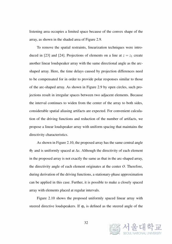
listening area occupies a limited space because of the convex shape of the
array, as shown in the shaded area of Figure 2.9.
To remove the spatial restraints, linearization techniques were intro-
duced in [23] and [24]. Projections of elements on a line at z = z1 create
another linear loudspeaker array with the same directional angle as the arc-
shaped array. Here, the time delays caused by projection differences need
to be compensated for in order to provide polar responses similar to those
of the arc-shaped array. As shown in Figure 2.9 by open circles, such pro-
jections result in irregular spaces between two adjacent elements. Because
the interval continues to widen from the center of the array to both sides,
considerable spatial aliasing artifacts are expected. For convenient calcula-
tion of the driving functions and reduction of the number of artifacts, we
propose a linear loudspeaker array with uniform spacing that maintains the
directivity characteristics.
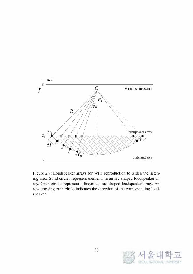
As shown in Figure 2.10, the proposed array has the same central angle
θT and is uniformly spaced at ∆x. Although the directivity of each element
in the proposed array is not exactly the same as that in the arc-shaped array,
the directivity angle of each element originates at the center O. Therefore,
during derivation of the driving functions, a stationary-phase approximation
can be applied in this case. Further, it is possible to make a closely spaced
array with elements placed at regular intervals.
Figure 2.10 shows the proposed uniformly spaced linear array with
steered directive loudspeakers. If ϕn is defined as the steered angle of the
32
x
z
z0
z1
z
Virtual sources area
Listening area
R
O
Δl
φn
θT
r1
rn
rN
Loudspeaker array
Figure 2.9: Loudspeaker arrays for WFS reproduction to widen the listen-ing area. Solid circles represent elements in an arc-shaped loudspeaker ar-ray. Open circles represent a linearized arc-shaped loudspeaker array. Ar-row crossing each circle indicates the direction of the corresponding loud-speaker.
33
z0
z1
z
R
O
φn
θT
r1
rn rN
Δx
Virtual sources area
Listening area
Loudspeaker array
x
z
Figure 2.10: Uniformly spaced linear array with directive loudspeakerssteered according to the arc-shaped array.
34
nth loudspeaker in the array, the synthesized sound field defined in (3.2)
(section 3.1.1) can be modified as
P(r,ω) =N∑
n=1
[Q(rn,ω)G(φn −ϕn,ω)
e− jk|r−rn|
|r− rn|
]∆x. (2.47)
Each directivity characteristic G in the driving functions for plane waves,
given by (3.3) in section 3.1.1, and focused sources, given by (3.6) in sec-
tion 3.1.2, should also be modified as
G(θ ′p,ω) = G(θp −ϕn,ω) (2.48)
and
G(θ ′n,ω) = G(θn −ϕn,ω), (2.49)
respectively.
2.3.2 Additional Sound Field Processing
To improve listeners’ spatial impressions, sound field processing may be
applied to the sound reproduction system. The proposed system adopts the
grouped reflection algorithm (GRA) [25, 26] for the additional processing.
As reported in [7], groups of reflections can be expanded to multiple groups
35

of loudspeaker channels in a WFS system. Therefore, the loudspeaker chan-
nels of the front array act as reflection groups that reproduce the early re-
flections in each direction in the system’s sound field processing stage.
36
Chapter 3
Spatial Sound Reproduction by
WFS
In this chapter, the sound reproduction method is discussed in terms of
its horizontal and vertical features. For sound reproduction on a horizon-
tal plane, a WFS-based sound reproduction technique that uses a front-only
loudspeaker array is proposed. To overcome the disadvantages of the ab-
sence of physical sound sources from the lateral and rear directions of the
listening area, a virtual surround algorithm based on focused source ren-
dering is proposed. The front array is shaped like a sound bar consisting of
equally spaced linear loudspeaker units for rendering virtual sound sources
by WFS. Each unit is steered divergently toward both ends of the array,
inspired by the process in arc-shaped loudspeaker arrays, to expand the lis-
tening area [13]. Moreover, double-layered loudspeaker arrays based on this
sound reproduction method are discussed for sound reproduction on a verti-
cal plane.
37
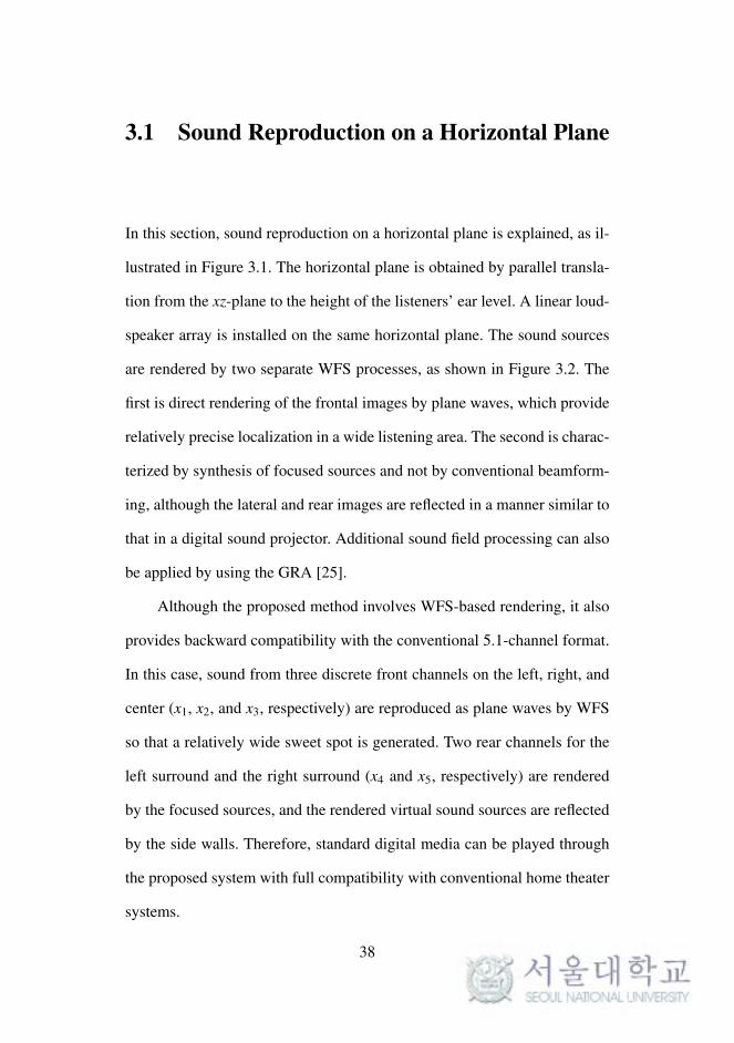
3.1 Sound Reproduction on a Horizontal Plane
In this section, sound reproduction on a horizontal plane is explained, as il-
lustrated in Figure 3.1. The horizontal plane is obtained by parallel transla-
tion from the xz-plane to the height of the listeners’ ear level. A linear loud-
speaker array is installed on the same horizontal plane. The sound sources
are rendered by two separate WFS processes, as shown in Figure 3.2. The
first is direct rendering of the frontal images by plane waves, which provide
relatively precise localization in a wide listening area. The second is charac-
terized by synthesis of focused sources and not by conventional beamform-
ing, although the lateral and rear images are reflected in a manner similar to
that in a digital sound projector. Additional sound field processing can also
be applied by using the GRA [25].
Although the proposed method involves WFS-based rendering, it also
provides backward compatibility with the conventional 5.1-channel format.
In this case, sound from three discrete front channels on the left, right, and
center (x1, x2, and x3, respectively) are reproduced as plane waves by WFS
so that a relatively wide sweet spot is generated. Two rear channels for the
left surround and the right surround (x4 and x5, respectively) are rendered
by the focused sources, and the rendered virtual sound sources are reflected
by the side walls. Therefore, standard digital media can be played through
the proposed system with full compatibility with conventional home theater
systems.
38
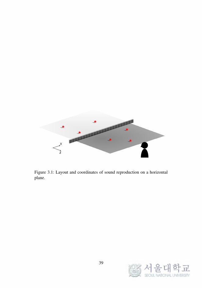
x
z
Figure 3.1: Layout and coordinates of sound reproduction on a horizontalplane.
39
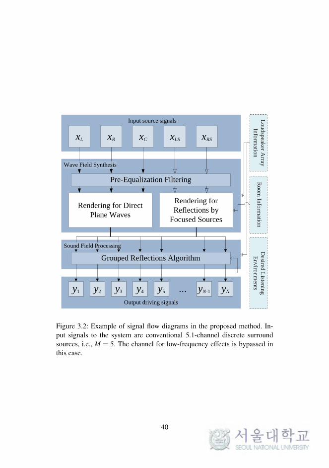
Input source signals
Output driving signals
Rendering for Direct
Plane Waves
Rendering for
Reflections by
Focused Sources
Pre-Equalization Filtering
xRSxLSxCxRxL
yN
Lou
dsp
eaker A
rray
Info
rmatio
n
Grouped Reflections Algorithm
Desired
Listen
ing
En
viro
nm
ents
Roo
m In
form
ation
yN-1…y1 y2 y3 y4 y5
Wave Field Synthesis
Sound Field Processing
Figure 3.2: Example of signal flow diagrams in the proposed method. In-put signals to the system are conventional 5.1-channel discrete surroundsources, i.e., M = 5. The channel for low-frequency effects is bypassed inthis case.
40
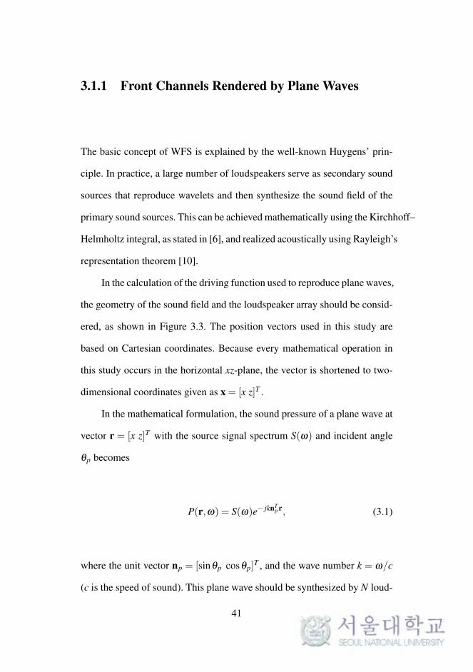
3.1.1 Front Channels Rendered by Plane Waves
The basic concept of WFS is explained by the well-known Huygens’ prin-
ciple. In practice, a large number of loudspeakers serve as secondary sound
sources that reproduce wavelets and then synthesize the sound field of the
primary sound sources. This can be achieved mathematically using the Kirchhoff–
Helmholtz integral, as stated in [6], and realized acoustically using Rayleigh’s
representation theorem [10].
In the calculation of the driving function used to reproduce plane waves,
the geometry of the sound field and the loudspeaker array should be consid-
ered, as shown in Figure 3.3. The position vectors used in this study are
based on Cartesian coordinates. Because every mathematical operation in
this study occurs in the horizontal xz-plane, the vector is shortened to two-
dimensional coordinates given as x = [x z]T .
In the mathematical formulation, the sound pressure of a plane wave at
vector r = [x z]T with the source signal spectrum S(ω) and incident angle
θp becomes
P(r,ω) = S(ω)e− jknTp r, (3.1)
where the unit vector np = [sinθp cosθp]T , and the wave number k = ω/c
(c is the speed of sound). This plane wave should be synthesized by N loud-
41
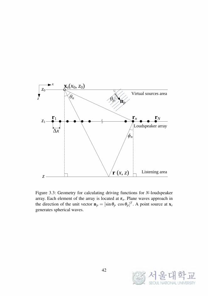
Loudspeaker array
z0
z1
z
ϕn
r1 rn rN
Δx
Virtual sources area
Listening area
x
z
xs(x0, z0)
r (x, z)
θn θp np
Figure 3.3: Geometry for calculating driving functions for N-loudspeakerarray. Each element of the array is located at rn. Plane waves approach inthe direction of the unit vector np = [sinθp cosθp]
T . A point source at xs
generates spherical waves.
42
speakers located on the z1-axis at a uniform interval ∆x according to
P(r,ω) =N∑
n=1
[Q(rn,ω)G(φn,ω)
e− jk|r−rn|
|r− rn|
]∆x, (3.2)
where Q(rn,ω) denotes the driving function of the nth loudspeaker to be
derived, and G(φn,ω) is the directivity characteristic. Further, rn denotes
the position vector of the nth loudspeaker element.
By means of the stationary-phase approximation as stated in [6], the
driving function can be derived without complex calculations as follows:
Q(rn,ω) = S(ω)
√cosθp
G(θp,ω)
√jk
2π
√|z− z1|e− jknT
p r. (3.3)
After the inverse Fourier transform of (3.3), a driving signal is obtained
in the time domain. This implies that the signal is realized computationally
by filtering, weighting, and delaying an input sound source signal in the
time domain. Because the term√
jk is a function only of the frequency,
it is simply applied to source signals as a pre-equalization filter before the
convolution in the rendering processes, as shown in Figure 3.2.
43
3.1.2 Virtual Surround Channels Obtained by Focused
Sources
Although rear loudspeakers need to be installed in order to reproduce the de-
sired spatial impression, it is practically difficult to install rear loudspeakers
at the positions defined in [2] in a domestic environment. For more conve-
nient installation, the proposed virtual surround method uses a front loud-
speaker array for the reproduction of rear-channel sound.
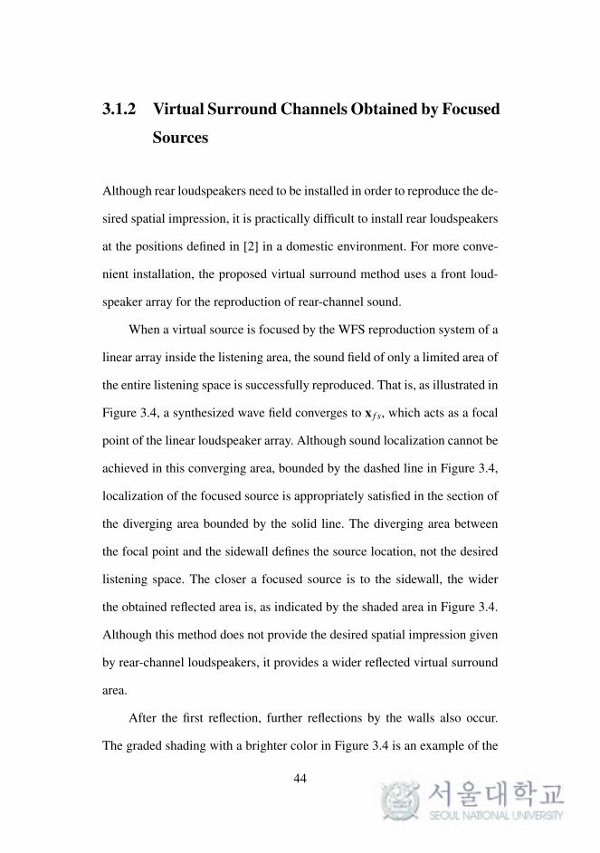
When a virtual source is focused by the WFS reproduction system of a
linear array inside the listening area, the sound field of only a limited area of
the entire listening space is successfully reproduced. That is, as illustrated in
Figure 3.4, a synthesized wave field converges to x f s, which acts as a focal
point of the linear loudspeaker array. Although sound localization cannot be
achieved in this converging area, bounded by the dashed line in Figure 3.4,
localization of the focused source is appropriately satisfied in the section of
the diverging area bounded by the solid line. The diverging area between
the focal point and the sidewall defines the source location, not the desired
listening space. The closer a focused source is to the sidewall, the wider
the obtained reflected area is, as indicated by the shaded area in Figure 3.4.
Although this method does not provide the desired spatial impression given
by rear-channel loudspeakers, it provides a wider reflected virtual surround
area.
After the first reflection, further reflections by the walls also occur.
The graded shading with a brighter color in Figure 3.4 is an example of the
44
z3
z1
Listening area
Loudspeaker arrayx
z
xfs(x2, z2)
Converging
Diverging
Reflected
Figure 3.4: Concept of virtual surround channel reproduction by reflectedfocused sources. The focal point is located at x f s = [x2 z2]
T . The left walland rear wall are shown on the x = 0 and z = z3 axes, respectively.
45

secondary reflections. Although it is impossible to eliminate such reflections
physically, it is worth noting that they do not influence the localization of
the perceived sound source in accordance with the precedence effect; the
delayed sounds are localized from the first arriving wavefront if successive
wavefronts arrive less than 50 ms after the first [12]. The time delay between
the first and second reflections is about 10 ms in a typical listening room.
Because the driving function for a focused source can be derived by
reversing the time in the driving function of a point source [9], the driv-
ing function of a point source at xs is calculated first. Similar to the plane
wave calculation for the reproduction of frontal images, the spherical wave
calculation for the focused source P(r,ω) is expressed as
P(r,ω) = S(ω)e− jk|r−xs|
|r−xs|, (3.4)
and the wave is synthesized according to (3.2). By a stationary-phase ap-
proximation, we obtain the driving function as
Q(rn,ω) = S(ω)cosθn
G(θn,ω)
√jk
2π
√|z− z1||z− z0|
e− jk|r−xs|
|r−xs|, (3.5)
where θn denotes the angle between the vertical line crossing xs and its
connection to the nth loudspeaker. If the focused source x f s and the point
46
source xs are symmetrical with the respect to the z1-axis, i.e.,
x f s(x0, z2) = [x0 2z1 − z0]T ,
the driving function of the focused source can be written as
Q(rn,ω) = S(ω)cosθn
G(θn,ω)
√− jk2π
√|z− z1||z− z2|
e jk|r−x f s|
|r−x f s|. (3.6)
During the implementation of this driving signal, an appropriate pre-delay
should be added not only to this reversed time delay but also to other driving
signals rendered by the plane waves to meet the causality condition and
obtain time synchronization.
3.2 Sound Reproduction on a Vertical Plane
In spatial audio reproduction, loudspeakers are usually arranged in the hori-
zontal plane. This restricts acoustic images to presentation on the projected
plane. To reproduce 3-D acoustic images, the horizontal plane of the loud-
speakers should be extended in the vertical direction using additional loud-
speakers. For example, 10.2- or 22.2-channel surround formats have an up-
per layer of loudspeakers to represent elevated images of sound sources
[4]. Although a binaural technique involving head-related transfer functions
47
could be used, the sound is reproduced only by headphones or earphones
for one person.
Similar to the conventional 5.1-channel surround system, the listening
area of interest is only the horizontal plane at the listener’s ear level in many
WFS systems. Thus, the planar array of loudspeakers could be reduced to
linear arrays because this does not affect the shape of the wavefronts in the
listener’s horizontal plane, as discussed in 2.1.4.
However, these loudspeaker arrangements could reproduce only sound
sources projected on the horizontal plane, as mentioned earlier. In this sec-
tion, double-layered loudspeaker arrays were used to reproduce virtual sources
expanded to a vertical plane in front of a listener. As shown in Figure 3.5, the
vertical plane is parallel to the xy-plane in front of the listener. A WFS-based
spatial sound rendering technique is proposed to localize virtual sources in
both azimuth and elevation. The typical WFS loudspeaker array is replaced
by a vertical panning image array of two loudspeaker layers above and be-
low the listener’s ear level.
3.2.1 3-D Vector Base Amplitude Panning
In 3-D sound impressions, the most important cue is the elevation of the
sound source. In addition to the proposed technique mentioned above, vec-
tor base amplitude panning (VBAP) is also used to compare the localization
quality of the two techniques. Three-dimensional VBAP is a generalization
of VBAP to three dimensions using three loudspeakers [27]. The virtual
48

xy
Figure 3.5: Layout and coordinates of sound reproduction on a verticalplane.
Figure 3.6: Example of 3-D VBAP
49
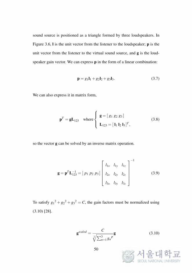
sound source is positioned as a triangle formed by three loudspeakers. In
Figure 3.6, l is the unit vector from the listener to the loudspeaker; p is the
unit vector from the listener to the virtual sound source, and g is the loud-
speaker gain vector. We can express p in the form of a linear combination:
p = g1l1 +g2l2 +g3l3. (3.7)
We can also express it in matrix form,
pT = gL123 where
g = [ g1 g2 g3 ]
L123 = [ l1 l2 l3 ]T ,(3.8)
so the vector g can be solved by an inverse matrix operation.
g = pT L−1123 = [ p1 p2 p3 ]
l1x l1y l1z
l2x l2y l2z
l3x l3y l3z
−1
(3.9)
To satisfy g12 + g2
2 + g32 = C, the gain factors must be normalized using
(3.10) [28].
gscaled =C
2√∑3
n=1 gnP
g (3.10)
50
3.2.2 Double-Layered Loudspeaker Arrays with 3-D
VBAP
In the 3-D VBAP rendering in the proposed double-layered system, triangles
formed by three loudspeakers are connected individually without intersect-
ing. A total of 12 loudspeakers (U1, U4, U7, U10, U13, U16, L1, L4, L7,
L10, L13, and L16) are used in the VBAP rendering, as shown in Figure 3.7.
The triangles are formed by two adjacent loudspeakers and the nearest loud-
speaker in the opposite side layer. Figure 3.7 shows a virtual sound source
S located on a triangle made of loudspeakers U4, L4, and L7.
VBAP is essentially a type of amplitude panning method using coher-
ent signals applied to loudspeakers. Thus, the loudspeaker positions must be
equidistant from the listening point. In this system, because the loudspeaker
arrays are straight lines on the frontal plane, the distances from the listener
to each loudspeaker vary with the position. Time delay compensation is nec-
essary in order to reproduce accurate virtual sources.
3.2.3 WFS Vertical Panning
An experiment was used to test elevation perception on the median plane us-
ing phantom images from two loudspeakers, as described in [29]. As shown
in Figure 3.8, the median of the perceived locations stayed close to 0 el-
evation with a small standard deviation until the inter-channel differences
moved beyond the halfway position, whereupon the perceived elevation
jumped to higher angles, although with a large standard deviation. For phan-
51
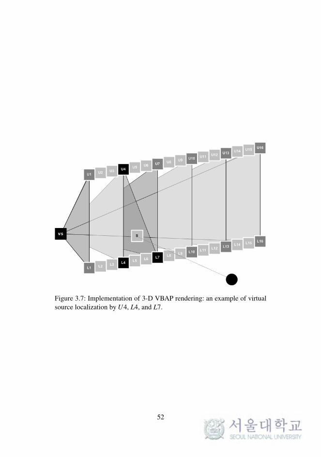
Figure 3.7: Implementation of 3-D VBAP rendering: an example of virtualsource localization by U4, L4, and L7.
52
tom images on the median plane with loudspeakers at 0 and 60, as shown
in Figure 3.9, the median of the perceived locations was again weighted to-
ward the 0 elevation loudspeaker until the inter-channel differences were
above the midpoint, with wider deviations in the central positions indicat-
ing a significant localization blur. There was also a consistent perception of
sources being toward the loudspeaker positions with a significant localiza-
tion blur for the central locations, as shown in Figure 3.10. Therefore, the
phantom images from two vertically separated loudspeakers are expected to
be adopted for vertical panning of two separate loudspeaker arrays, notwith-
standing some localization blur.
First, a 2-D wave field is synthesized by a virtual loudspeaker array
located between two real array layers. Each column, consisting of an upper
and lower loudspeaker pair, generates a virtual loudspeaker, and the eleva-
tion vectors of each loudspeaker are calculated from the layout of the virtual
source and the upper and lower loudspeaker pairs. Then each virtual loud-
speaker signal is extended to the real upper and lower loudspeaker pairs
by amplitude panning using the elevation vectors. Only vertical amplitude
panning was used because horizontal acoustic images are localized by 2-D
WFS.
The concept of 3-D expansion is illustrated in Figure 3.11. The ren-
dered secondary source S on the horizontal plane (2-D) is panned to the
upper layer of U and the lower layer of L. In practice, because the distance
from virtual source V S to each loudspeaker differs, the exact elevation of
53
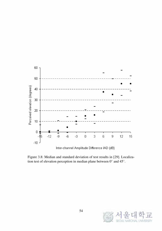
Figure 3.8: Median and standard deviation of test results in [29]. Localiza-tion test of elevation perception in median plane between 0 and 45.
54
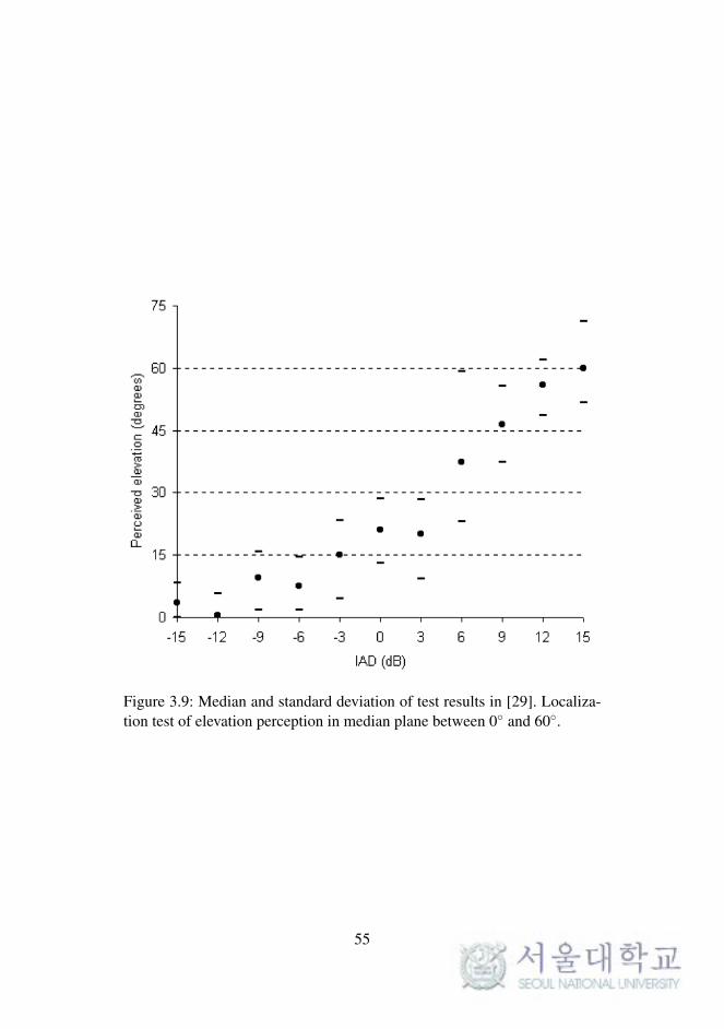
Figure 3.9: Median and standard deviation of test results in [29]. Localiza-tion test of elevation perception in median plane between 0 and 60.
55
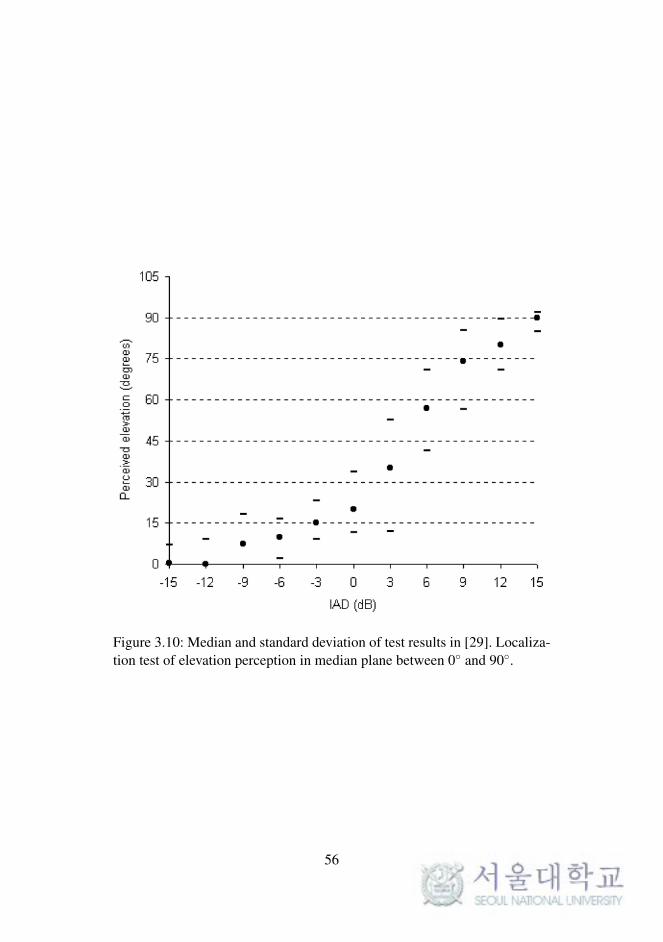
Figure 3.10: Median and standard deviation of test results in [29]. Localiza-tion test of elevation perception in median plane between 0 and 90.
56
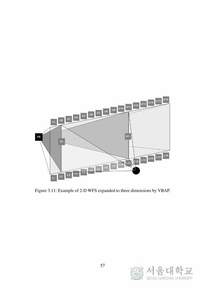
Figure 3.11: Example of 2-D WFS expanded to three dimensions by VBAP.
57
the secondary sources may differ like that for S2 and S11 in Figure 3.11.
Moreover, if VBAP is used for vertical panning, the location of the listen-
ing point should be the basis for calculating vectors from the listener to the
virtual sound source.
However, sound images were already localized on the horizontal plane;
only the vertical component from the locations of the sound source and the
listener was considered for the 3-D expansion model. Thus, the virtual sound
source was located using the vertical components in the amplitude panning
method based on the arrangement. Figure 3.12 represents the final concept
of WFS vertical panning (VP) for 3-D expansion.
58
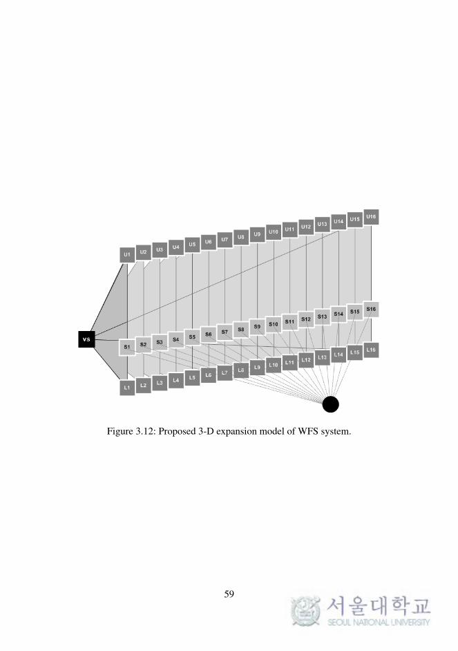
Figure 3.12: Proposed 3-D expansion model of WFS system.
59

60
Chapter 4
Implementation and Simulations
4.1 Specifications of Implemented System
Implementation of the proposed system for UHDTV was considered. Be-
cause the resolution of UHDTV is 16 times better than that of HDTV, the
diagonal screen size was assumed to be 100 in. for the accompanying linear
loudspeaker array. At an aspect ratio of 16:9, the horizontal length of the
screen is restricted to almost 2,200 mm (87 in.). Because the proposed ar-
ray consists of 24 loudspeaker units having a diameter of 69.9 mm (2¾ in.),
loudspeakers were arranged at intervals of 89 mm. For a double-layered
loudspeaker array setup for vertical reproduction, 32 loudspeaker units were
arranged at intervals of 170 mm. Each layer had 16 loudspeaker units, and
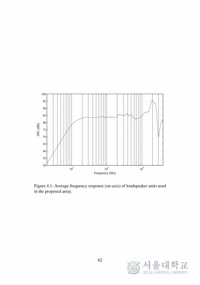
the layers were vertically separated by 1,650 mm in height. The average
measured frequency response of the loudspeaker units used in this system
is plotted in Figure 4.1. The measurement microphone was placed on the
axis 1.0 m from the center of the units. The loudspeaker arrays were driven
by six sets of ROTEL RMB-1066 power amps. Audio signals were gener-
61
102
103
104
50
55
60
65
70
75
80
85
90
95
100
SP
L (
dB)
Frequency (Hz)
Figure 4.1: Average frequency response (on-axis) of loudspeaker units usedin the proposed array.
62
ated and played using a MATLAB program through four units of the MOTU
896HD interface.
4.1.1 Pre-Equalization Filter
Because the diameter of the loudspeaker units was not sufficiently large, the
low-frequency response had a cutoff frequency of less than 200 Hz. This fre-
quency characteristic was considered in the pre-filter design. As discussed in
Chapter 3, a pre-equalization filter was required for the input source signals
before the rendering process. The term√
jk acted as a 3-dB/octave high-
pass filter in the frequency domain. Accordingly, the overall low-frequency
response below the cutoff frequency of the proposed method weakened.
Therefore, a flat response was applied to the pre-equalization filter below
the cutoff frequency.
In [30, 9], the pre-equalization filter was defined in the context of the
spherical wave source. If the virtual sound source location is not sufficiently
far (|(r)s − (r)n| ≫ 1) behind the loudspeaker array, the distance from the
virtual sound source to the loudspeaker should be considered when calcu-
lating the pre-equalization filter:
fSW (t) = F−1
(1√
j ω
c |rn − rm|+
√jω
c
). (4.1)
Consequently, the design of the pre-equalization filter should depend on the
63
characteristics of the virtual sources and the frequency response of the loud-
speakers.
4.2 Simulations and Results
4.2.1 Simulation Methods
To illustrate the sound field reproduced by the proposed methods, computa-
tional simulations were performed. Omnidirectional monopole elements are
generally considered as point sources in simulations of array processing.
However, these point sources were not adequate for the simulations of the
proposed method because each element had a different directivity in the pro-
posed array. Furthermore, a monopole source could not approximate the di-
rectivity pattern of a loudspeaker because the directivity of the loudspeaker
increased as the frequency increased. An approximation for the radiation of
the loudspeaker is given by the plane circular piston model in [17] as
P(r,φ) = jρcπa
J1(kasinφ)
rsinφe− jkr, (4.2)
where r is the distance from the center of the piston, φ is the angle from
the axis of the piston, a is the radius of the piston, J1(·) denotes the Bessel
function of the first kind of order 1, and ρ is the density of the medium.
In the simulations of the proposed system, this plane circular piston model
was used to calculate the sound pressure in the synthesized sound field. An
64
acoustic model built using the image method [31] was used to analyze the re-
flections by the sidewalls in the simulation of virtual surround channels. The
principal concern was the situation around a single sidewall during reflec-
tion by a synthesized focused source. Hence, the image method considered
the left wall during the simulations of the virtual left surround channel. The
reflections by the rear and right walls were also considered, and reflections
up to the second order were simulated. The sound absorbing characteris-
tics of the walls were also considered in the simulations. We considered the
Sabine absorptivity [17] when simulating the wall reflection.
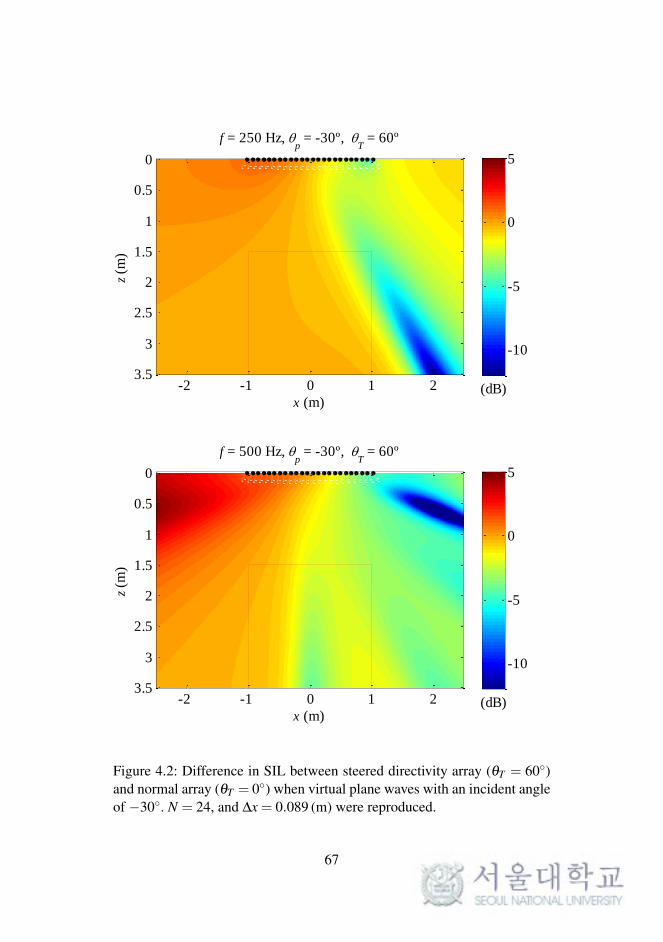
4.2.2 Simulations of Steered Array
In this section, the simulated sound fields are represented in order to com-
pare the steered directivity angles in the array. We consider the difference
in the sound intensity level (SIL) distribution between the steered directiv-
ity array with central angle θT and the normal array. The sound field was
simulated computationally for a typical listening room (dimensions: 5.0 m
× 3.5 m). For a clear comparison of the direct plane waves rendered by dif-
ferently steered arrays, the reflections from the walls were ignored in these
simulations. The implemented loudspeaker array was configured such that
it was located at the top center of each plot, i.e., on the line at z = 0 and
−1.02 5 x 5 1.02, with a uniform interval of 0.089 m. The listening area
was determined according to the viewing distances recommended in [2],
which are a minimum distance of 1.5 m from the display and a maximum
65
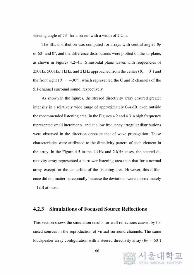
viewing angle of 73 for a screen with a width of 2.2 m.
The SIL distribution was computed for arrays with central angles θT
of 60 and 0, and the difference distributions were plotted on the xz-plane,
as shown in Figures 4.2–4.5. Sinusoidal plane waves with frequencies of
250 Hz, 500 Hz, 1 kHz, and 2 kHz approached from the center (θp = 0) and
the front right (θp =−30), which represented the C and R channels of the
5.1-channel surround sound, respectively.
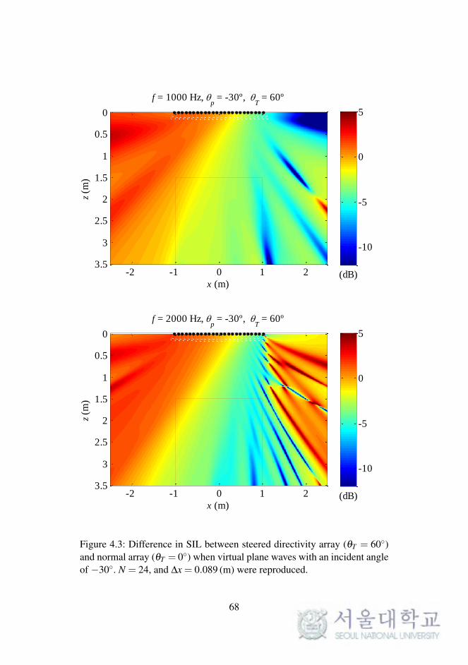
As shown in the figures, the steered directivity array ensured greater
intensity in a relatively wide range of approximately 0–4 dB, even outside
the recommended listening area. In the Figures 4.2 and 4.3, a high frequency
represented small increments, and at a low frequency, irregular distributions
were observed in the direction opposite that of wave propagation. These
characteristics were attributed to the directivity pattern of each element in
the array. In the Figure 4.5 in the 1-kHz and 2-kHz cases, the steered di-
rectivity array represented a narrower listening area than that for a normal
array, except for the centerline of the listening area. However, this differ-
ence did not matter perceptually because the deviations were approximately
−1 dB at most.
4.2.3 Simulations of Focused Source Reflections
This section shows the simulation results for wall reflections caused by fo-
cused sources in the reproduction of virtual surround channels. The same
loudspeaker array configuration with a steered directivity array (θT = 60)
66
f = 250 Hz, p = -30º,
T = 60º
x (m)
z (m
)
-2 -1 0 1 2
0
0.5
1
1.5
2
2.5
3
3.5 (dB)
-10
-5
0
5
f = 500 Hz, p = -30º,
T = 60º
x (m)
z (m
)
-2 -1 0 1 2
0
0.5
1
1.5
2
2.5
3
3.5 (dB)
-10
-5
0
5
Figure 4.2: Difference in SIL between steered directivity array (θT = 60)and normal array (θT = 0) when virtual plane waves with an incident angleof −30. N = 24, and ∆x = 0.089 (m) were reproduced.
67
f = 1000 Hz, p = -30º,
T = 60º
x (m)
z (m
)
-2 -1 0 1 2
0
0.5
1
1.5
2
2.5
3
3.5 (dB)
-10
-5
0
5
f = 2000 Hz, p = -30º,
T = 60º
x (m)
z (m
)
-2 -1 0 1 2
0
0.5
1
1.5
2
2.5
3
3.5 (dB)
-10
-5
0
5
Figure 4.3: Difference in SIL between steered directivity array (θT = 60)and normal array (θT = 0) when virtual plane waves with an incident angleof −30. N = 24, and ∆x = 0.089 (m) were reproduced.
68

f = 250 Hz, p = 0º,
T = 60º
x (m)
z (m
)
-2 -1 0 1 2
0
0.5
1
1.5
2
2.5
3
3.5 (dB)
-2
-1.5
-1
-0.5
0
0.5
1
f = 500 Hz, p = 0º,
T = 60º
x (m)
z (m
)
-2 -1 0 1 2
0
0.5
1
1.5
2
2.5
3
3.5 (dB)
-2
-1.5
-1
-0.5
0
0.5
1
Figure 4.4: Difference in SIL between steered directivity array (θT = 60)and normal array (θT = 0) when virtual plane waves with an incident angleof 0. N = 24, and ∆x = 0.089 (m) were reproduced.
69

f = 1000 Hz, p = 0º,
T = 60º
x (m)
z (m
)
-2 -1 0 1 2
0
0.5
1
1.5
2
2.5
3
3.5 (dB)
-2
-1.5
-1
-0.5
0
0.5
1
f = 2000 Hz, p = 0º,
T = 60º
x (m)
z (m
)
-2 -1 0 1 2
0
0.5
1
1.5
2
2.5
3
3.5 (dB)
-2
-1.5
-1
-0.5
0
0.5
1
Figure 4.5: Difference in SIL between steered directivity array (θT = 60)and normal array (θT = 0) when virtual plane waves with an incident angleof 0. N = 24, and ∆x = 0.089 (m) were reproduced.
70

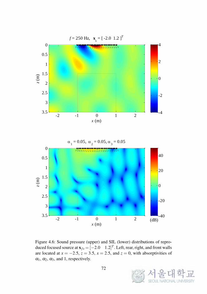
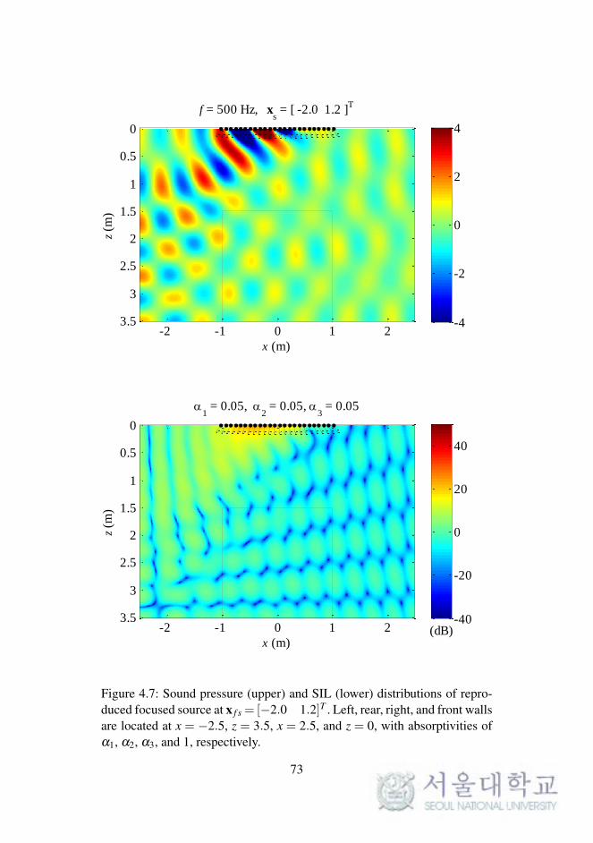
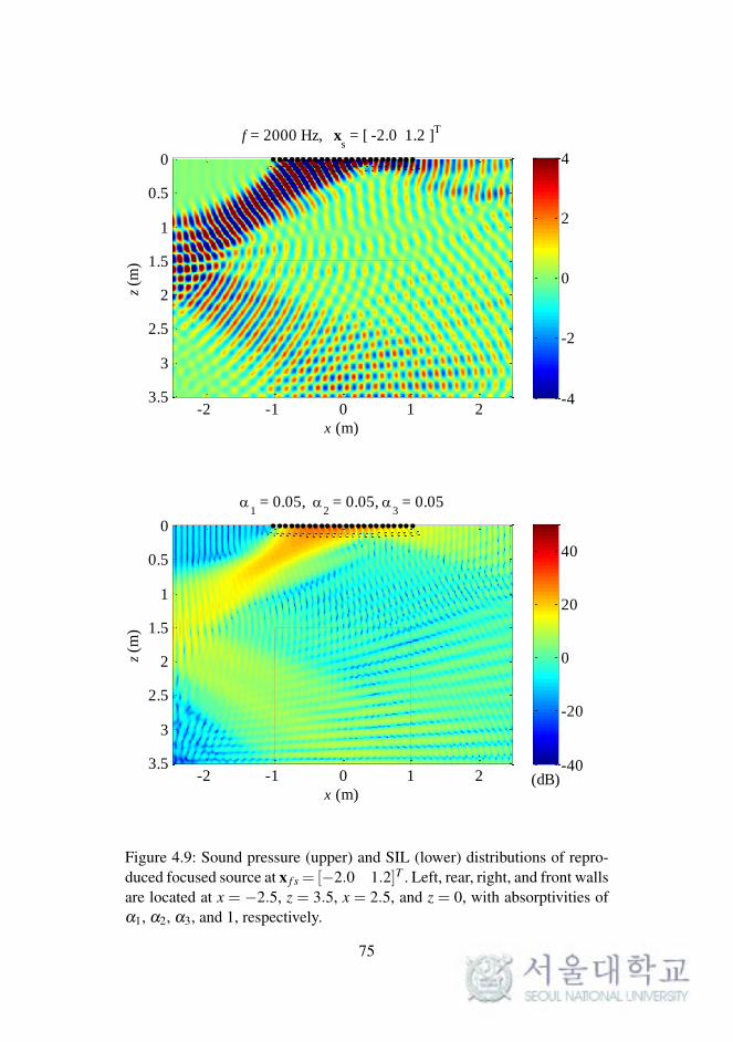
was used. The sound pressure distributions of the reproduced focused source
are presented in Figures 4.6–4.9. In each figure, the upper panel shows the
real values of the simulated sound pressure field, and the lower panel shows
the corresponding intensity level field. The sidewall for the main reflection
was on the left of the listening room, as shown on the axis at x = −2.5.
The rear and right walls were located on the axis at z = 3.5 and x = 2.5, re-
spectively. The absorptivity values of the left, rear, and right walls (α1, α2,
and α3, respectively) were determined to be 0.05, assuming normal wooden
walls. The front wall was considered to be absorptive with an absorptiv-
ity value of 1. Because the reproduction system is generally attached to the
front wall, each loudspeaker becomes a dipole; hence, the reflections from
the front wall become a problem of level normalization.
A focused source was located at x f s = [−2 1.2]T , close to the left wall;
hence, the incident angle was approximately 60. As shown in the bounded
listening area in the figures, the desired sound field was synthesized by the
left wall. Further, a high-frequency focused source (Figure 4.9) produced
a narrower beam than a low-frequency one in a similar beamforming pro-
cess. Because of interference by the second-order reflections from the rear
wall, several nodes were observed in the results. Although they may cause
sound coloration, the sound localization still matches, as discussed in Sec-
tion 3.1.2. A possible solution for this problem is to make the rear wall a
diffuse or absorptive surface.
71
f = 250 Hz, xs = [ -2.0 1.2 ]
T
x (m)
z (m
)
-2 -1 0 1 2
0
0.5
1
1.5
2
2.5
3
3.5
-4
-2
0
2
4
1 = 0.05,
2 = 0.05,
3 = 0.05
x (m)
z (m
)
-2 -1 0 1 2
0
0.5
1
1.5
2
2.5
3
3.5 (dB)
-40
-20
0
20
40
Figure 4.6: Sound pressure (upper) and SIL (lower) distributions of repro-duced focused source at x f s = [−2.0 1.2]T . Left, rear, right, and front wallsare located at x = −2.5, z = 3.5, x = 2.5, and z = 0, with absorptivities ofα1, α2, α3, and 1, respectively.
72
f = 500 Hz, xs = [ -2.0 1.2 ]
T
x (m)
z (m
)
-2 -1 0 1 2
0
0.5
1
1.5
2
2.5
3
3.5
-4
-2
0
2
4
1 = 0.05,
2 = 0.05,
3 = 0.05
x (m)
z (m
)
-2 -1 0 1 2
0
0.5
1
1.5
2
2.5
3
3.5 (dB)
-40
-20
0
20
40
Figure 4.7: Sound pressure (upper) and SIL (lower) distributions of repro-duced focused source at x f s = [−2.0 1.2]T . Left, rear, right, and front wallsare located at x = −2.5, z = 3.5, x = 2.5, and z = 0, with absorptivities ofα1, α2, α3, and 1, respectively.
73

f = 1000 Hz, xs = [ -2.0 1.2 ]
T
x (m)
z (m
)
-2 -1 0 1 2
0
0.5
1
1.5
2
2.5
3
3.5
-4
-2
0
2
4
1 = 0.05,
2 = 0.05,
3 = 0.05
x (m)
z (m
)
-2 -1 0 1 2
0
0.5
1
1.5
2
2.5
3
3.5 (dB)
-40
-20
0
20
40
Figure 4.8: Sound pressure (upper) and SIL (lower) distributions of repro-duced focused source at x f s = [−2.0 1.2]T . Left, rear, right, and front wallsare located at x = −2.5, z = 3.5, x = 2.5, and z = 0, with absorptivities ofα1, α2, α3, and 1, respectively.
74
f = 2000 Hz, xs = [ -2.0 1.2 ]
T
x (m)
z (m
)
-2 -1 0 1 2
0
0.5
1
1.5
2
2.5
3
3.5
-4
-2
0
2
4
1 = 0.05,
2 = 0.05,
3 = 0.05
x (m)
z (m
)
-2 -1 0 1 2
0
0.5
1
1.5
2
2.5
3
3.5 (dB)
-40
-20
0
20
40
Figure 4.9: Sound pressure (upper) and SIL (lower) distributions of repro-duced focused source at x f s = [−2.0 1.2]T . Left, rear, right, and front wallsare located at x = −2.5, z = 3.5, x = 2.5, and z = 0, with absorptivities ofα1, α2, α3, and 1, respectively.
75
4.2.4 Simulations of Double-Layered Arrays
In WFS, as described in Chapter 2, the synthesized sound field on a 2-D
plane was considered. The reproduced sound images on a horizontal or ver-
tical plane were expanded to 3-D space, as described in the previous chapter.
To synthesize the 3-D sound field directly, the loudspeaker arrays should be
implemented as planar arrays surrounding the listening area.
In this section, the sound field reproduced by double-layered loud-
speaker arrays in the computational simulations is presented. The simula-
tions compared the sound fields reproduced by loudspeaker arrays and the
desired point source. The method of simulating the 2-D sound field used in
the previous section is extended to three dimensions.
For ease of visualization, the 3-D sound field was plotted using com-
binations of sliced orthogonal planes according to the listener’s position. In
Figures 4.10–4.24, three planes are displayed: the xy-plane at z = 0, the xz-
plane at y = 1.1, and the yz-plane at x = 0. The xz-plane at a height of 1.1
was selected because ear level at the listening point was 1.1 m from the floor
of the listening room.
As expected, the horizontal resolution of the simulation results on the
xz-plane closely resembled that of the desired point source. As shown in
the vertical intersection crossing the median plane of the listener, the syn-
thesized sound field had small errors when the virtual source was close to
the height of each array. For virtual sources located between the two arrays,
several pressure nodes were observed under the influence of spatial aliasing
76
in the yz-plane. Because of these nodes, correct sound at listening positions
of varying heights would not be guaranteed because they might cause sound
coloration. However, it does not matter that the sound field was distorted on
the vertical plane because listeners are generally located at listening posi-
tions of constant height.
77
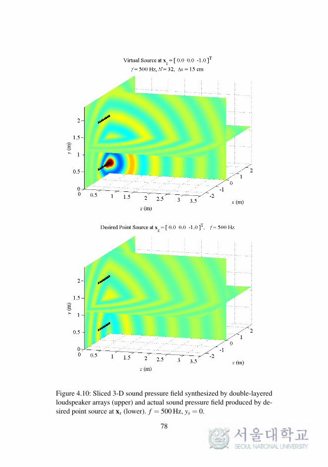
Figure 4.10: Sliced 3-D sound pressure field synthesized by double-layeredloudspeaker arrays (upper) and actual sound pressure field produced by de-sired point source at xs (lower). f = 500 Hz, ys = 0.
78
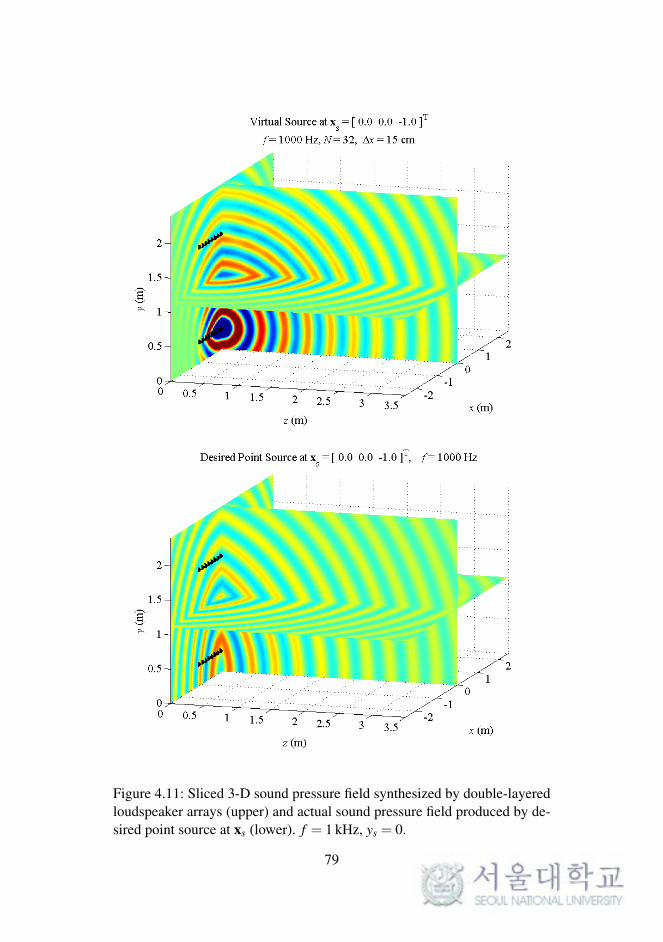
Figure 4.11: Sliced 3-D sound pressure field synthesized by double-layeredloudspeaker arrays (upper) and actual sound pressure field produced by de-sired point source at xs (lower). f = 1 kHz, ys = 0.
79
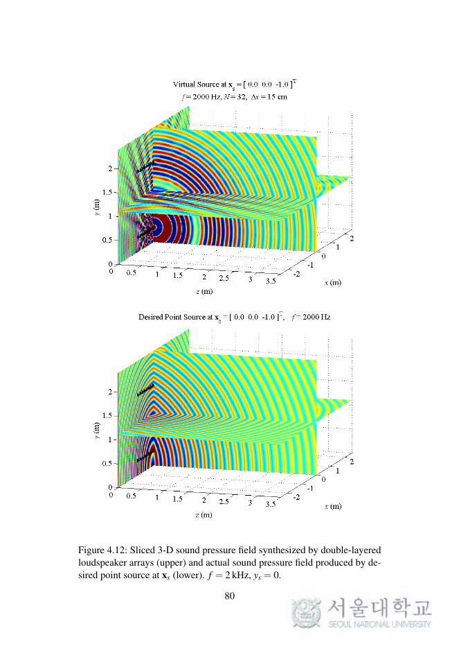
Figure 4.12: Sliced 3-D sound pressure field synthesized by double-layeredloudspeaker arrays (upper) and actual sound pressure field produced by de-sired point source at xs (lower). f = 2 kHz, ys = 0.
80
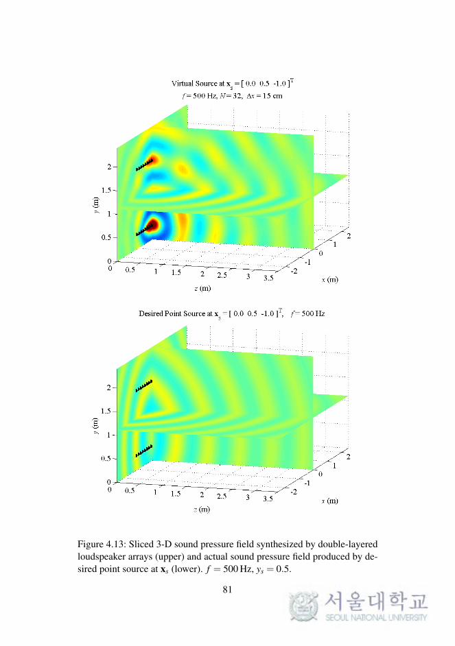
Figure 4.13: Sliced 3-D sound pressure field synthesized by double-layeredloudspeaker arrays (upper) and actual sound pressure field produced by de-sired point source at xs (lower). f = 500 Hz, ys = 0.5.
81
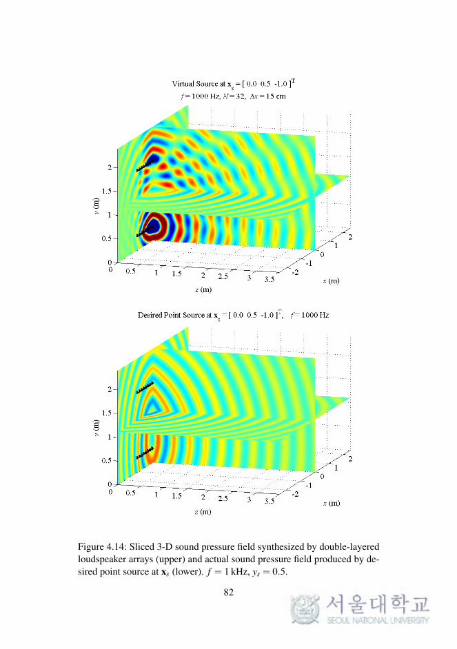
Figure 4.14: Sliced 3-D sound pressure field synthesized by double-layeredloudspeaker arrays (upper) and actual sound pressure field produced by de-sired point source at xs (lower). f = 1 kHz, ys = 0.5.
82
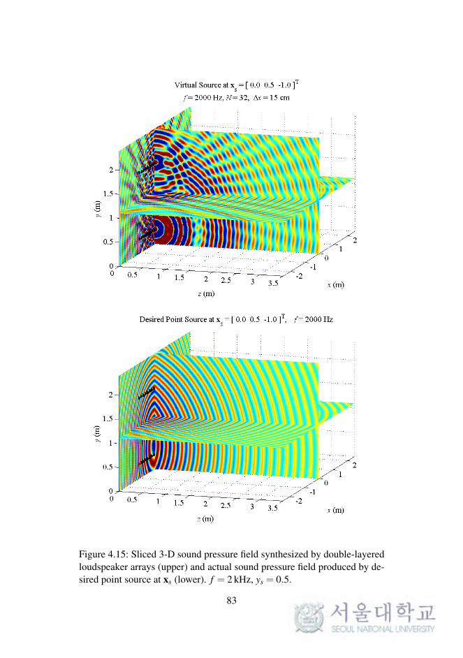
Figure 4.15: Sliced 3-D sound pressure field synthesized by double-layeredloudspeaker arrays (upper) and actual sound pressure field produced by de-sired point source at xs (lower). f = 2 kHz, ys = 0.5.
83

Figure 4.16: Sliced 3-D sound pressure field synthesized by double-layeredloudspeaker arrays (upper) and actual sound pressure field produced by de-sired point source at xs (lower). f = 500 Hz, ys = 1.0.
84
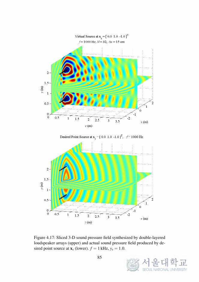
Figure 4.17: Sliced 3-D sound pressure field synthesized by double-layeredloudspeaker arrays (upper) and actual sound pressure field produced by de-sired point source at xs (lower). f = 1 kHz, ys = 1.0.
85
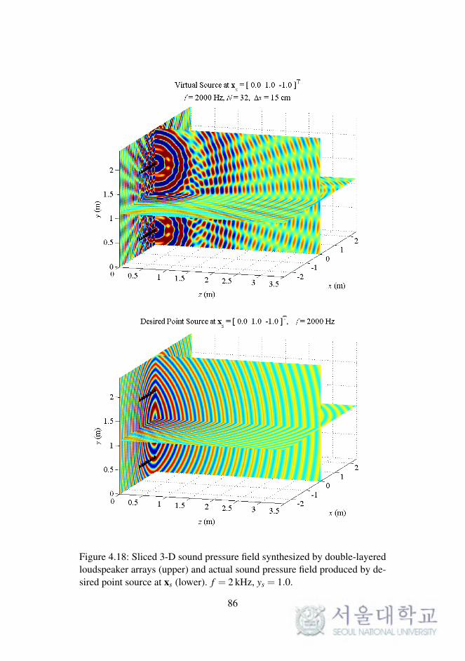
Figure 4.18: Sliced 3-D sound pressure field synthesized by double-layeredloudspeaker arrays (upper) and actual sound pressure field produced by de-sired point source at xs (lower). f = 2 kHz, ys = 1.0.
86
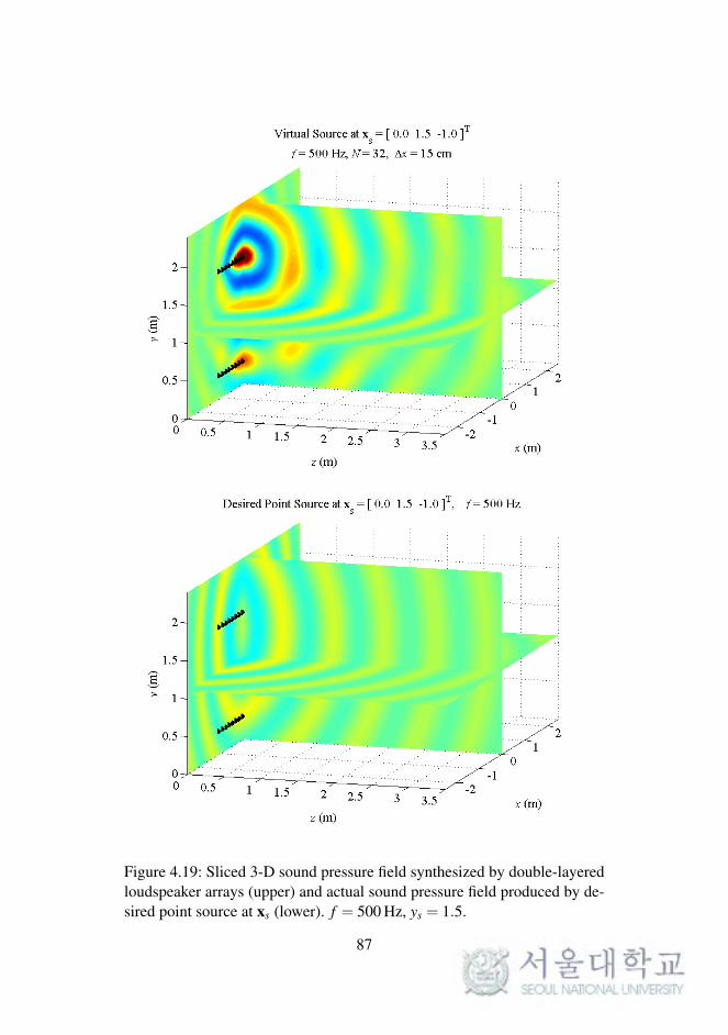
Figure 4.19: Sliced 3-D sound pressure field synthesized by double-layeredloudspeaker arrays (upper) and actual sound pressure field produced by de-sired point source at xs (lower). f = 500 Hz, ys = 1.5.
87
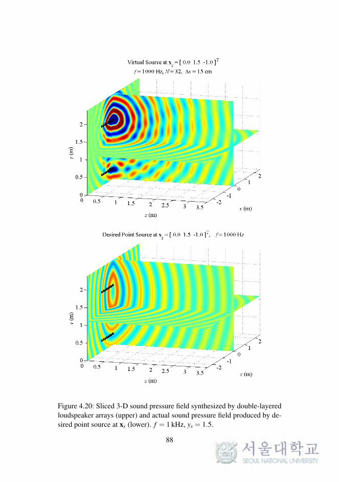
Figure 4.20: Sliced 3-D sound pressure field synthesized by double-layeredloudspeaker arrays (upper) and actual sound pressure field produced by de-sired point source at xs (lower). f = 1 kHz, ys = 1.5.
88
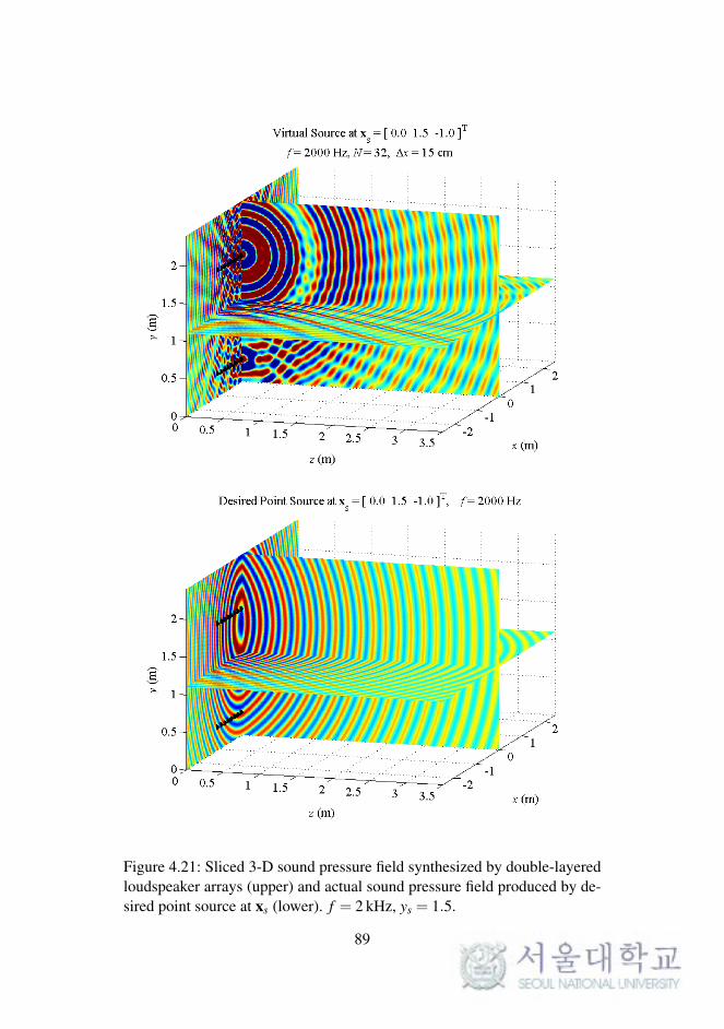
Figure 4.21: Sliced 3-D sound pressure field synthesized by double-layeredloudspeaker arrays (upper) and actual sound pressure field produced by de-sired point source at xs (lower). f = 2 kHz, ys = 1.5.
89

Figure 4.22: Sliced 3-D sound pressure field synthesized by double-layeredloudspeaker arrays (upper) and actual sound pressure field produced by de-sired point source at xs (lower). f = 500 Hz, ys = 2.0.
90

Figure 4.23: Sliced 3-D sound pressure field synthesized by double-layeredloudspeaker arrays (upper) and actual sound pressure field produced by de-sired point source at xs (lower). f = 1 kHz, ys = 2.0.
91
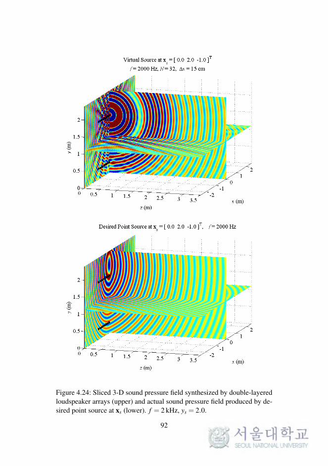
Figure 4.24: Sliced 3-D sound pressure field synthesized by double-layeredloudspeaker arrays (upper) and actual sound pressure field produced by de-sired point source at xs (lower). f = 2 kHz, ys = 2.0.
92
4.3 Subjective Assessment
Subjective listening tests [32] were conducted to evaluate the frontal lo-
calization in the proposed system. Although localization experiments using
various spatial reproduction systems were performed in [33, 34], the WFS
systems in these experiments remained in the horizontal plane. In this sec-
tion, both horizontal and vertical localization tests were performed [35, 36,
37].
For the horizontal localization test, a single layer of a linear loud-
speaker array in front of a listener was used. For the vertical test, a double-
layered loudspeaker array was used. In the first experiment in 4.3.1, the
accuracy of the listening test system was verified. In a second experiment
in 4.3.2, a frontal localization test using 3-D VBAP [28] was conducted for
comparison with the proposed rendering method, and the frontal localiza-
tion of the proposed WFS rendering method was evaluated.
4.3.1 Horizontal Localization
In this section, subjective tests of sound localization were executed to in-
spect the performance of the localization quality of the implemented linear
loudspeaker array system. Virtual sound images were rendered as spherical
point sources by the proposed WFS method. All the sound sources were lo-
cated virtually on a horizontal plane in front of a listener. The system was
implemented with a 24-channel linear loudspeaker array located in front of
the listening area. Loudspeaker units were spaced 0.15 m from each other.
93
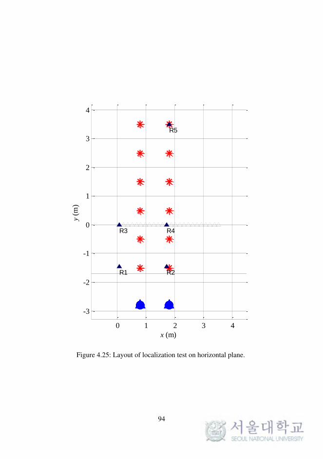
0 1 2 3 4
-3
-2
-1
0
1
2
3
4
x (m)
y (m
)
R1 R2
R3 R4
R5
Figure 4.25: Layout of localization test on horizontal plane.
94

4.3.1.1 Test environment
The localization tests were conducted in the listening room at the Institute
of New Media & Communication, Seoul National University. The room di-
mensions are 4.7 m × 5.3 m × 2.4 m. The reverberation time (RT60) is 0.32
s at 1 kHz. Figure 4.25 shows a floor view of the test layout. Two additional
physical loudspeakers were installed for use as reference sound sources.
Furthermore, an acoustically transparent blind curtain was drawn in front of
the listening area at y = −1.6. Therefore, subjects could be isolated from
possible sources of visual bias.
4.3.1.2 Subject test panel
Eleven male and female subjects ranging in age from 20 to 31 participated
in the experiment. All the subjects had previous localization test experience
and no hearing problems.
4.3.1.3 Stimuli
Two sound sources were used in the localization experiments. The first was
pink noise bursts 3 s in duration. The second was a piece of music played
by the cello and recorded in an anechoic chamber. Each sound source was
rendered at 12 different virtual locations, indicated in Figure 4.25 by red
asterisks.
95
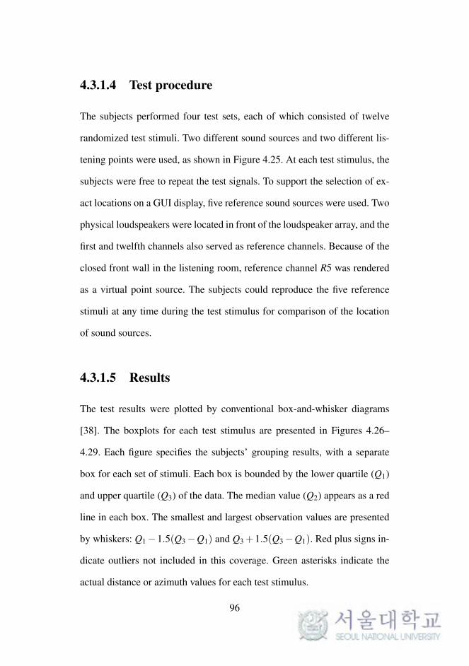
4.3.1.4 Test procedure
The subjects performed four test sets, each of which consisted of twelve
randomized test stimuli. Two different sound sources and two different lis-
tening points were used, as shown in Figure 4.25. At each test stimulus, the
subjects were free to repeat the test signals. To support the selection of ex-
act locations on a GUI display, five reference sound sources were used. Two
physical loudspeakers were located in front of the loudspeaker array, and the
first and twelfth channels also served as reference channels. Because of the
closed front wall in the listening room, reference channel R5 was rendered
as a virtual point source. The subjects could reproduce the five reference
stimuli at any time during the test stimulus for comparison of the location
of sound sources.
4.3.1.5 Results
The test results were plotted by conventional box-and-whisker diagrams
[38]. The boxplots for each test stimulus are presented in Figures 4.26–
4.29. Each figure specifies the subjects’ grouping results, with a separate
box for each set of stimuli. Each box is bounded by the lower quartile (Q1)
and upper quartile (Q3) of the data. The median value (Q2) appears as a red
line in each box. The smallest and largest observation values are presented
by whiskers: Q1 −1.5(Q3 −Q1) and Q3 +1.5(Q3 −Q1). Red plus signs in-
dicate outliers not included in this coverage. Green asterisks indicate the
actual distance or azimuth values for each test stimulus.
96
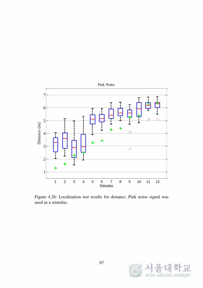
1
2
3
4
5
6
7
Pink Noise
1 2 3 4 5 6 7 8 9 10 11 12Stimulus
Dis
tan
ce (
m)
Figure 4.26: Localization test results for distance. Pink noise signal wasused as a stimulus.
97
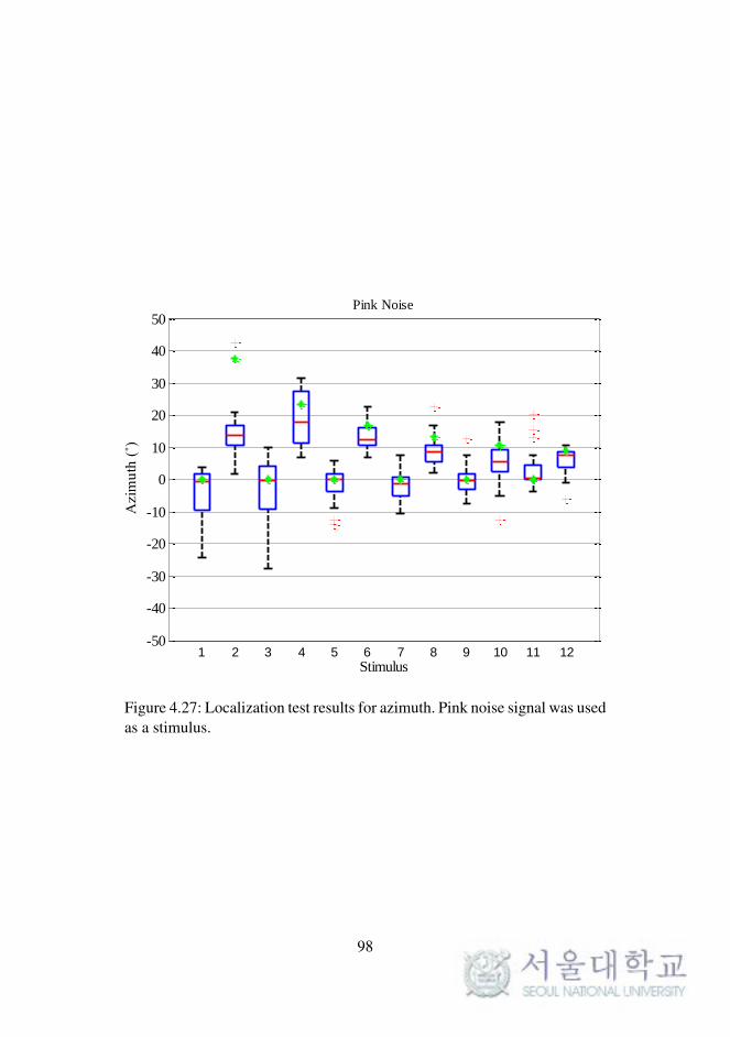
-50
-40
-30
-20
-10
0
10
20
30
40
50Pink Noise
1 2 3 4 5 6 7 8 9 10 11 12Stimulus
Azim
uth
(˚)
Figure 4.27: Localization test results for azimuth. Pink noise signal was usedas a stimulus.
98
1
2
3
4
5
6
7
Music
1 2 3 4 5 6 7 8 9 10 11 12Stimulus
Dis
tan
ce (
m)
Figure 4.28: Localization test results for distance. Musical signal was usedas a stimulus.
99
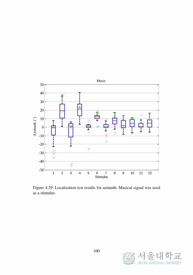
-50
-40
-30
-20
-10
0
10
20
30
40
50Music
1 2 3 4 5 6 7 8 9 10 11 12Stimulus
Azim
uth
(˚)
Figure 4.29: Localization test results for azimuth. Musical signal was usedas a stimulus.
100
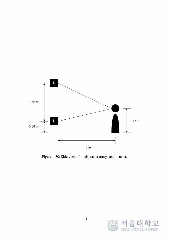
Figure 4.30: Side view of loudspeaker arrays and listener.
101

4.3.2 Vertical Localization
In this section, the proposed double-layered loudspeaker arrays were used
to reproduce virtual sources on the vertical plane in front of a listener. The
system was built up with 32-channel loudspeakers. Each array had 16 loud-
speakers spaced 0.17 m apart. The two layers were separated by 1.65 m
in height. The lower layer stood 0.34 m above the floor, as shown in Fig-
ure 4.30. To produce a convenient test procedure for subjects, a grid refer-
ence consisting of colored strings at intervals of about 30 cm was placed on
the vertical plane of the loudspeaker arrays.
4.3.2.1 Test environment
The localization tests were conducted in the listening room described in
4.3.1. The subjects sat on a chair 2 m away from the center of the loud-
speaker array (Figure 4.30). The subjects were free to move their heads dur-
ing the test.
4.3.2.2 Subject test panel
Five male subjects ranging in age from 24 to 33 participated in the experi-
ment. All the subjects had previous localization test experience and no hear-
ing problems.
102

4.3.2.3 Stimuli
Two sound sources were used for the localization experiments. The first was
pink noise bursts 3 s in duration. The second consisted of mixed sounds of
a bicycle bell and a ratchet. Each source was rendered by the WFS VP and
3-D VBAP methods.
4.3.2.4 Reference experiment for vertical localization
A reference experiment was done before the localization tests. It was de-
signed to investigate how accurately the subjects recognized the positions
of loudspeakers when the virtual sources were located exactly at the loud-
speaker positions. Subjects were asked to identify the position of virtual
sources located on the frontal area between two loudspeaker arrays, al-
though real sources existed only at the loudspeaker array positions. The
same pink noise stimulus as in the localization test was used. A random
set of 20 loudspeaker channels was used in each test. A new random set of
channels was generated for each subject. In each reference test set, over-
lapping of the loudspeaker channels was avoided. Subjects could repeat the
test signals until they reached a decision. During the listening tests, subjects
used a test program implemented in MATLAB. They entered the numbers
of the perceived loudspeaker until the test ended.
103
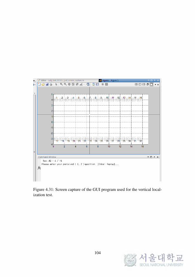
Figure 4.31: Screen capture of the GUI program used for the vertical local-ization test.
104
4.3.2.5 Test procedure
Fifteen virtual sound source positions were used during the localization
tests. All the test procedures used random test sets. In each set, the vir-
tual sound source positions were assigned randomly. A new random set of
virtual source positions was generated for each subject, as in the reference
experiment. The positions of the virtual sound sources had five different
elevations and three different azimuths in a 5× 3 matrix form. All virtual
sound sources were rendered as located 1 m behind the plane made by the
loudspeaker arrays. The horizontal positions were −1.2 m, 0 m, and +1.2 m
from the center. The vertical positions were −0.8 m, −0.4 m, 0 m, +0.4 m,
and +0.8 m from the center. The test results for the virtual source positions
on the right (+0.4 m and +0.8 m) were converted to the left side using the
symmetry with respect to the median plane. In each test, subjects listened to
the test stimulus and then identified the location of the sound source using
a GUI program implemented in MATLAB, as shown in Figure 4.31. Sub-
jects could repeat the same test stimulus until they reached a decision, as in
the reference experiment. The GUI program displayed the loudspeaker ar-
rangements on-screen, along with the same grid imposed on the loudspeaker
arrays. Subjects moved a cursor on the screen using a mouse and clicked
when they made a decision. After the first localization test, the same pro-
cedure was repeated with the other sound source (bicycle bell and ratchet
sounds).
105
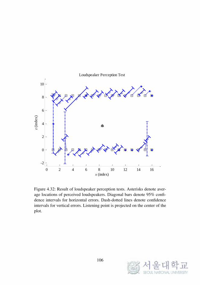
0 2 4 6 8 10 12 14 16
-2
0
2
4
6
8
10
x (index)
z (i
nd
ex
)
Loudspeaker Perception Test
Figure 4.32: Result of loudspeaker perception tests. Asterisks denote aver-age locations of perceived loudspeakers. Diagonal bars denote 95% confi-dence intervals for horizontal errors. Dash-dotted lines denote confidenceintervals for vertical errors. Listening point is projected on the center of theplot.
106
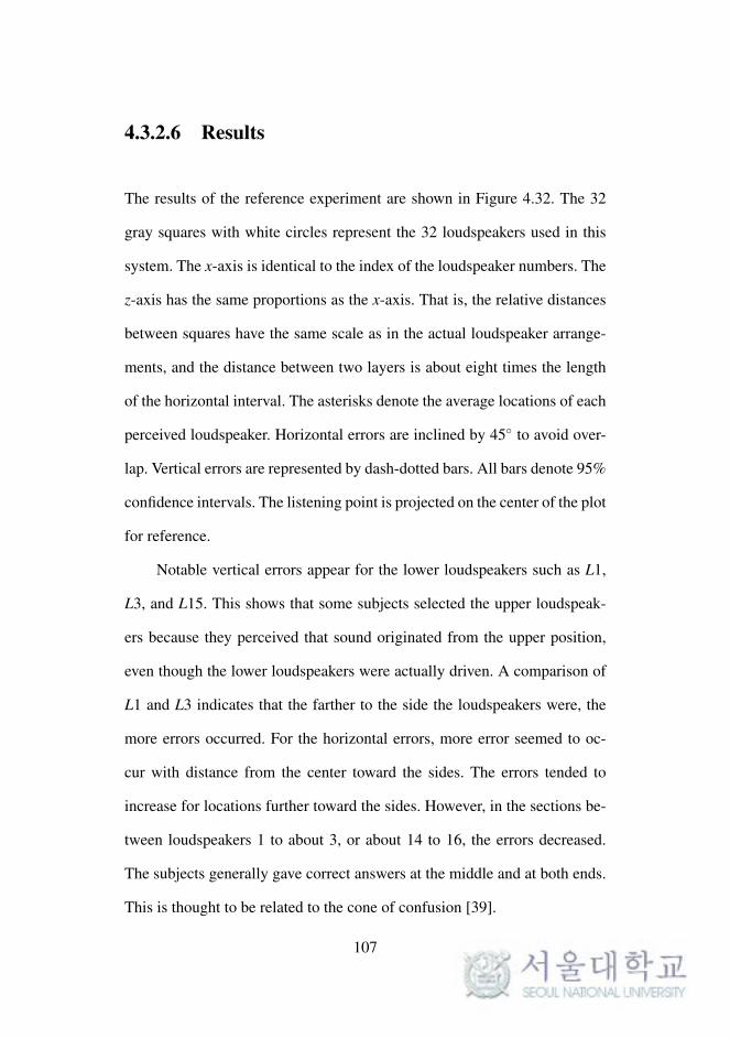
4.3.2.6 Results
The results of the reference experiment are shown in Figure 4.32. The 32
gray squares with white circles represent the 32 loudspeakers used in this
system. The x-axis is identical to the index of the loudspeaker numbers. The
z-axis has the same proportions as the x-axis. That is, the relative distances
between squares have the same scale as in the actual loudspeaker arrange-
ments, and the distance between two layers is about eight times the length
of the horizontal interval. The asterisks denote the average locations of each
perceived loudspeaker. Horizontal errors are inclined by 45 to avoid over-
lap. Vertical errors are represented by dash-dotted bars. All bars denote 95%
confidence intervals. The listening point is projected on the center of the plot
for reference.
Notable vertical errors appear for the lower loudspeakers such as L1,
L3, and L15. This shows that some subjects selected the upper loudspeak-
ers because they perceived that sound originated from the upper position,
even though the lower loudspeakers were actually driven. A comparison of
L1 and L3 indicates that the farther to the side the loudspeakers were, the
more errors occurred. For the horizontal errors, more error seemed to oc-
cur with distance from the center toward the sides. The errors tended to
increase for locations further toward the sides. However, in the sections be-
tween loudspeakers 1 to about 3, or about 14 to 16, the errors decreased.
The subjects generally gave correct answers at the middle and at both ends.
This is thought to be related to the cone of confusion [39].
107
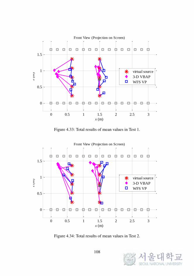
0 0.5 1 1.5 2 2.5 3
0
0.5
1
1.5
Front View (Projection on Screen)
x (m)
z (m
)
virtual source
3-D VBAP
WFS VP
Figure 4.33: Total results of mean values in Test 1.
0 0.5 1 1.5 2 2.5 3
0
0.5
1
1.5
Front View (Projection on Screen)
x (m)
z (m
)
virtual source
3-D VBAP
WFS VP
Figure 4.34: Total results of mean values in Test 2.
108
The results of the localization tests are presented in Figures 4.33 and
4.34. In test 1, a pink noise signal was used for the virtual sound sources, and
a bicycle bell and ratchet sounds were used for test 2, as described above.
In most results for the WFS VP method, the resolution in the horizontal
direction was quite accurate. However, in the test of 3-D VBAP, the side
results were slightly further from the intended sound source. This seems to
be related to the characteristics of VBAP. The secondary images made by
three loudspeakers are located only on the triangular plane made by the three
loudspeakers. Thus, the lateral virtual sources reproduced by our system
might be projected toward the screen in the normal direction, not along the
direction of the listening point. This can be recognized in the specific results
presented in Figures 4.35–4.44. In both methods, the results were clustered
toward the center of the vertical direction. Although the WFS VP results
could be classified by elevation, the VBAP results were somewhat poor.
In test 2, there was a notable tendency that most results were biased
close to the upper loudspeaker layer. This is more remarkable in the VBAP
results. Subjects were confused regarding the exact elevation because some
subjects felt that the sound was separated into upper and lower layers or
altered as they moved their eyes. This is believed to be related to the spec-
trum of the signal used in test 2. The tonal component of the signal might
act as a spectral cue for judging the elevation [40, 41]. Thus, test 2 was not
as successful as test 1, although it was intended to provide familiar sound
signals.
109
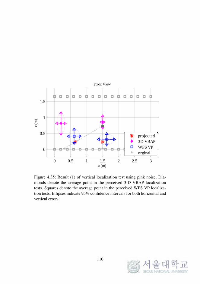
0 0.5 1 1.5 2 2.5 3
0
0.5
1
1.5
x (m)
z (
m)
Front View
projected
3D VBAP
WFS VP
orginal
Figure 4.35: Result (1) of vertical localization test using pink noise. Dia-monds denote the average point in the perceived 3-D VBAP localizationtests. Squares denote the average point in the perceived WFS VP localiza-tion tests. Ellipses indicate 95% confidence intervals for both horizontal andvertical errors.
110
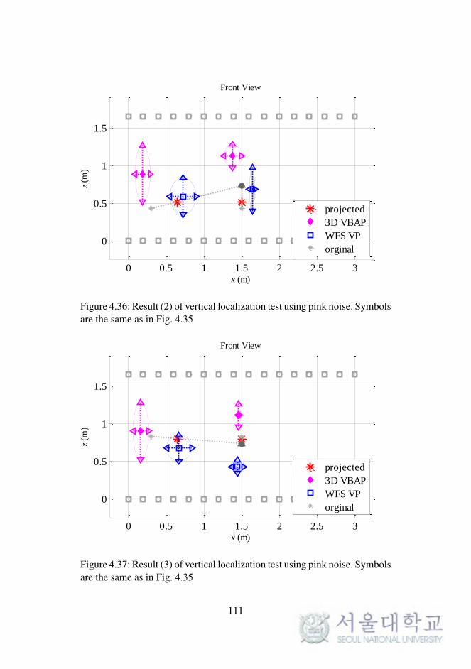
0 0.5 1 1.5 2 2.5 3
0
0.5
1
1.5
x (m)
z (
m)
Front View
projected
3D VBAP
WFS VP
orginal
Figure 4.36: Result (2) of vertical localization test using pink noise. Symbolsare the same as in Fig. 4.35
0 0.5 1 1.5 2 2.5 3
0
0.5
1
1.5
x (m)
z (
m)
Front View
projected
3D VBAP
WFS VP
orginal
Figure 4.37: Result (3) of vertical localization test using pink noise. Symbolsare the same as in Fig. 4.35
111
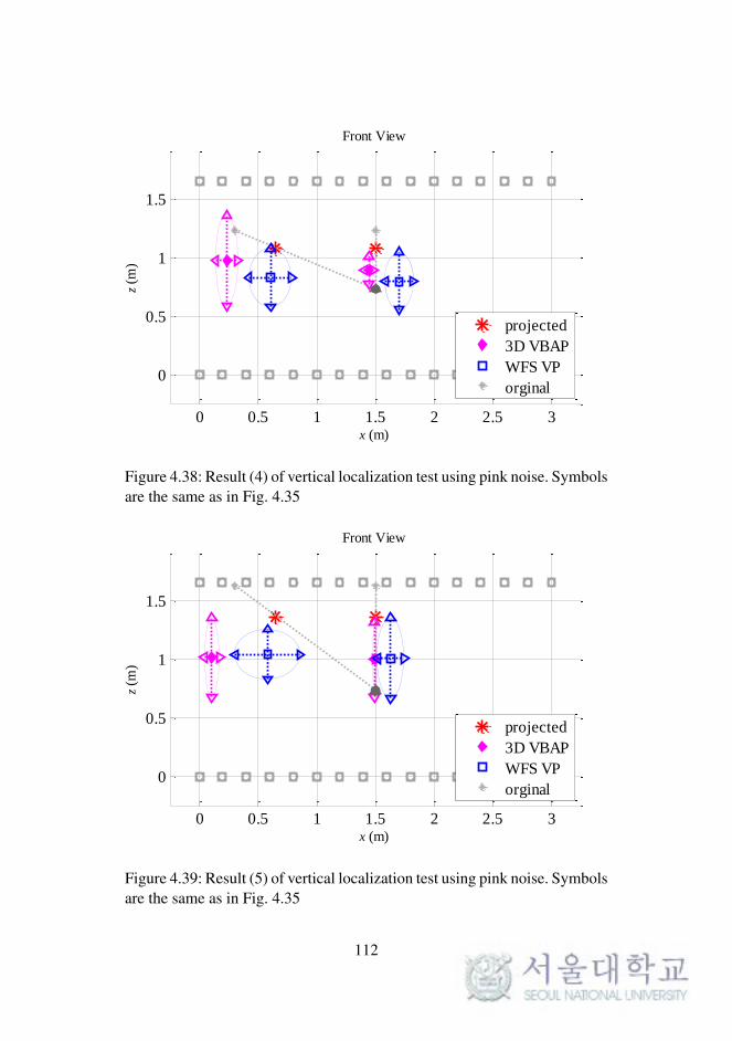
0 0.5 1 1.5 2 2.5 3
0
0.5
1
1.5
x (m)
z (
m)
Front View
projected
3D VBAP
WFS VP
orginal
Figure 4.38: Result (4) of vertical localization test using pink noise. Symbolsare the same as in Fig. 4.35
0 0.5 1 1.5 2 2.5 3
0
0.5
1
1.5
x (m)
z (
m)
Front View
projected
3D VBAP
WFS VP
orginal
Figure 4.39: Result (5) of vertical localization test using pink noise. Symbolsare the same as in Fig. 4.35
112
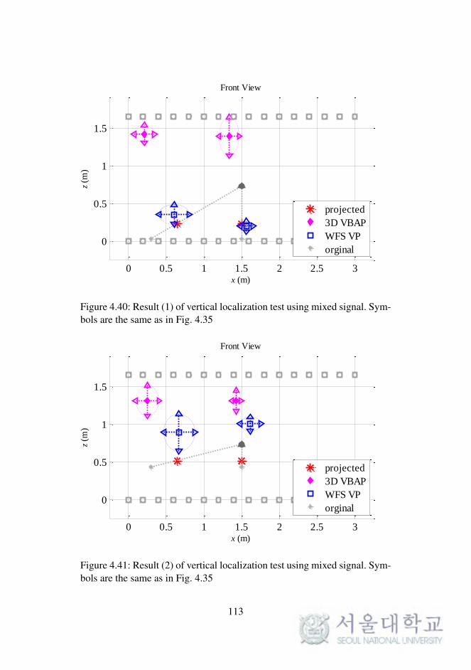
0 0.5 1 1.5 2 2.5 3
0
0.5
1
1.5
x (m)
z (
m)
Front View
projected
3D VBAP
WFS VP
orginal
Figure 4.40: Result (1) of vertical localization test using mixed signal. Sym-bols are the same as in Fig. 4.35
0 0.5 1 1.5 2 2.5 3
0
0.5
1
1.5
x (m)
z (
m)
Front View
projected
3D VBAP
WFS VP
orginal
Figure 4.41: Result (2) of vertical localization test using mixed signal. Sym-bols are the same as in Fig. 4.35
113
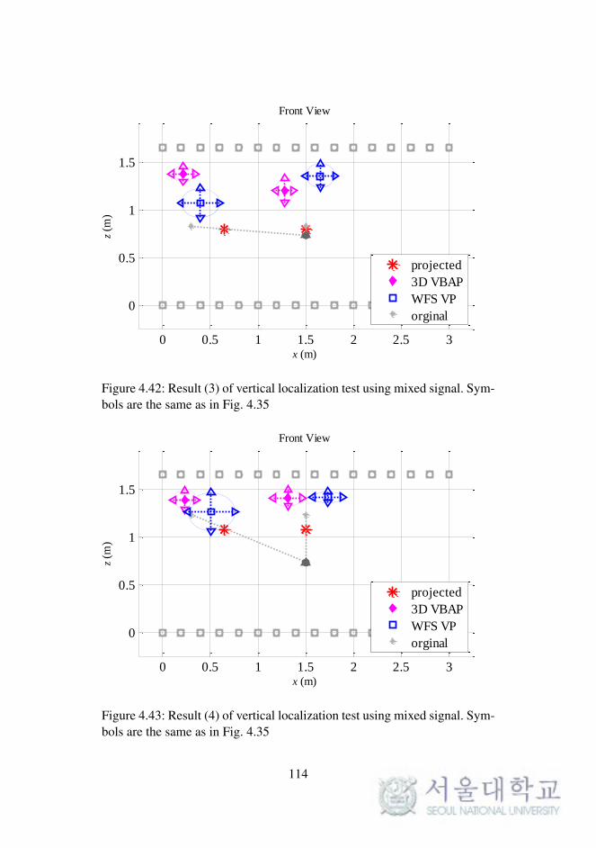
0 0.5 1 1.5 2 2.5 3
0
0.5
1
1.5
x (m)
z (
m)
Front View
projected
3D VBAP
WFS VP
orginal
Figure 4.42: Result (3) of vertical localization test using mixed signal. Sym-bols are the same as in Fig. 4.35
0 0.5 1 1.5 2 2.5 3
0
0.5
1
1.5
x (m)
z (
m)
Front View
projected
3D VBAP
WFS VP
orginal
Figure 4.43: Result (4) of vertical localization test using mixed signal. Sym-bols are the same as in Fig. 4.35
114
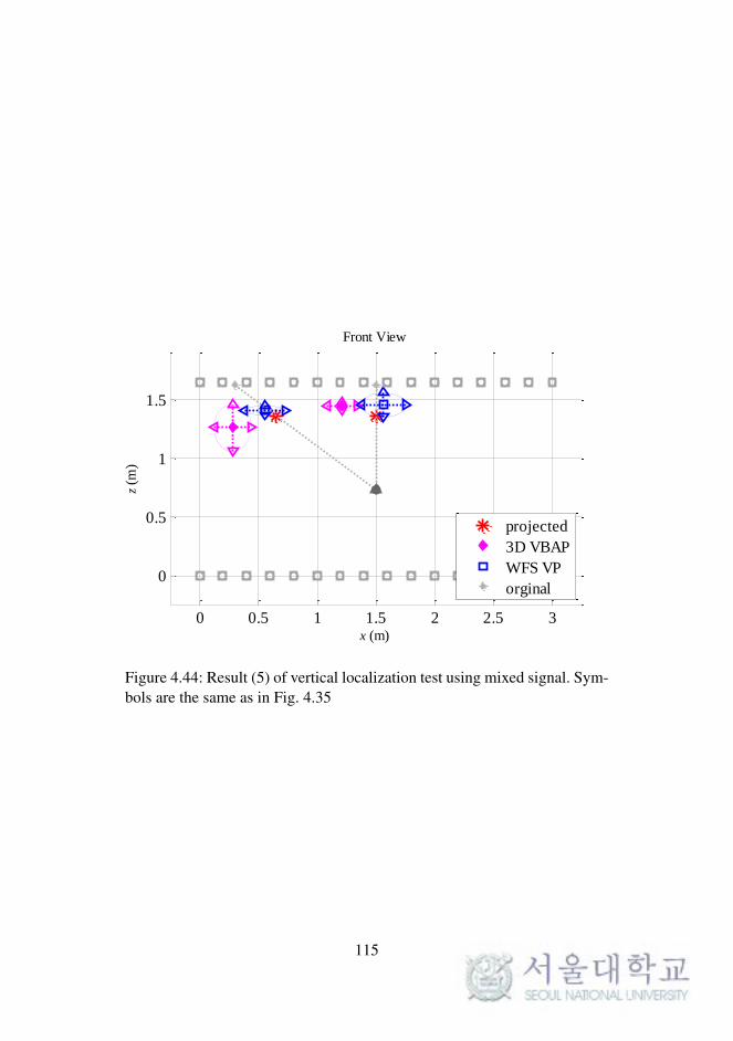
0 0.5 1 1.5 2 2.5 3
0
0.5
1
1.5
x (m)
z (
m)
Front View
projected
3D VBAP
WFS VP
orginal
Figure 4.44: Result (5) of vertical localization test using mixed signal. Sym-bols are the same as in Fig. 4.35
115
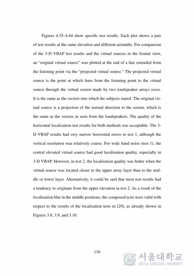
Figures 4.35–4.44 show specific test results. Each plot shows a pair
of test results at the same elevation and different azimuths. For comparison
of the 3-D VBAP test results and the virtual sources in the frontal view,
an “original virtual source” was plotted at the end of a line extended from
the listening point via the “projected virtual source.” The projected virtual
source is the point at which lines from the listening point to the virtual
source through the virtual screen made by two loudspeaker arrays cross.
It is the same as the vectors into which the subjects stared. The original vir-
tual source is a projection of the normal direction to the screen, which is
the same as the vectors as seen from the loudspeakers. The quality of the
horizontal localization test results for both methods was acceptable. The 3-
D VBAP results had very narrow horizontal errors in test 1, although the
vertical resolution was relatively coarse. For wide band noise (test 1), the
central elevated virtual source had good localization quality, especially in
3-D VBAP. However, in test 2, the localization quality was better when the
virtual source was located closer to the upper array layer than to the mid-
dle or lower layer. Alternatively, it could be said that most test results had
a tendency to originate from the upper elevation in test 2. As a result of the
localization blur in the middle positions, the composed tests were valid with
respect to the results of the localization tests in [29], as already shown in
Figures 3.8, 3.9, and 3.10.
116
Chapter 5
Conclusion
In this dissertation, an improved sound reproduction technique was pro-
posed that uses front linear loudspeaker arrays that can be installed with
a display device. The frontal sound images are rendered as plane waves us-
ing WFS. For virtual sound sources from lateral directions, focused sources
were rendered by WFS and reflected by sidewalls. An equally spaced lin-
ear loudspeaker array with steered directivity along the arc direction was
proposed to extend the optimum listening area. Furthermore, a WFS render-
ing method using a double-layered loudspeaker array was also studied. A
WFS VP method was proposed to expand the sound images on the horizon-
tal plane to three dimensions. On the basis of conventional WFS methods,
WFS VP generates a virtual loudspeaker array between two real loudspeaker
layers and reproduces them by vertical amplitude panning. A 3-D VBAP
method was also studied and implemented appropriately for this system’s
loudspeaker arrangement.
The results of computational simulations demonstrated that the SILs
117
of the sides of the listening area were widened by about 0–5 dB. The imple-
mented system showed potential for installation as consumer electronics.
Subject tests were conducted to evaluate the localization quality of this sys-
tem. A comparison of 3-D VBAP and WFS VP revealed good horizontal
localization resolution in both systems. The WFS VP system was some-
what better than the 3-D VBAP system. However, large errors in the ver-
tical localization quality occurred in both systems, although WFS VP had
relatively small variances. The results showed that it is feasible to expand
2-D sound images to 3-D images having both azimuth and elevation using
a double-layered WFS array system, although errors occurred in the per-
ception of clear virtual images in the 3-D field. To compare the algorithms
more accurately, it remains as future work to calibrate the 3-D VBAP ren-
dering algorithm in this system. Subjective listening test procedures using
psychoacoustical methods will also be studied to obtain more robust ex-
periments. The proposed system is expected to be a useful application for
next-generation home theater systems.
118
Bibliography
[1] Audio Engineering Society, An anthology of reprinted articles on
stereophonic techniques. New York: Audio Engineering Society, 1986.
[2] “Multichannel stereophonic sound system with and without accompa-
nying picture,” Recommendation ITU-R BS 775-1, 1994.
[3] “IOSONO,” Comput. Entertain., vol. 2, no. 3, 2004.
[4] K. Hamasaki, T. Nishiguchi, R. Okumura, Y. Nakayama, and A. Ando,
“A 22.2 multichannel sound system for Ultrahigh-Definition TV
(UHDTV),” SMPTE Motion Imaging Journal, vol. 117, no. 4, pp. 40–
49, 2008.
[5] A. J. Berkhout, “A holographic approach to acoustic control,” Journal
of the Audio Engineering Society, vol. 36, no. 12, pp. 977–995, 1988.
[6] A. J. Berkhout, D. de Vries, and P. Vogel, “Acoustic control by wave
field synthesis,” Journal of the Acoustical Society of America, vol. 93,
no. 5, pp. 2764–2778, 1993.
[7] H. Chung, J. Lim, H. Shim, K.-M. Sung, and J.-h. Yoo, “Hybrid sound
field processing for wave field synthesis system,” in Audio Engineer-
ing Society 122nd Convention, (Vienna), Audio Engineering Society,
2007.
[8] M. M. Boone, E. N. G. Verheijen, and P. F. van Tol, “Spatial sound-
field reproduction by wave-field synthesis,” J. Audio Eng. Soc, vol. 43,
no. 12, pp. 1003–1012, 1995.
[9] S. Spors, H. Wierstorf, M. Geier, and J. Ahrens, “Physical and percep-
tual properties of focused sources in wave field synthesis,” in Audio
Engineering Society 127th Convention, (New York), 2009.
119
[10] D. de Vries, Wave field synthesis. New York: Audio Engineering So-
ciety, 2009.
[11] T. Hooley, “Single box surround sound,” Acoustical Science and Tech-
nology, vol. 27, no. 6, pp. 354–360, 2006.
[12] J. Blauert, Spatial hearing : the psychophysics of human sound local-
ization. Cambridge, Mass.: MIT Press, rev. ed., 1997.
[13] H. Chung, H. Shim, N. Hahn, S. B. Chon, and K.-M. Sung, “Sound re-
production method by front loudspeaker array for home theater appli-
cations,” IEEE Transactions on Consumer Electronics, vol. 58, no. 2,
pp. 528 –534, 2012.
[14] R. D. Finch, Introduction to acoustics. Upper Saddle River, NJ: Pear-
son, 1st ed., 2005.
[15] S. Spors, H. Teutsch, and R. R., “High-quality acoustic rendering with
wave field synthesis,” in Vision, Modelling and Visualization (VMV),
pp. 101–108, 11 2002.
[16] E. G. Williams, Fourier acoustics : sound radiation and nearfield
acoustical holography. Academic Press, 1999.
[17] L. E. Kinsler, A. R. Frey, A. B. Coppens, and J. V. Sanders, Funda-
mentals of acoustics. New York: Wiley, 4th ed., 2000.
[18] D. de Vries, “Sound reinforcement by wavefield synthesis: Adaptation
of the synthesis operator to the loudspeaker directivity characteristics,”
J. Audio Eng. Soc, vol. 44, no. 12, pp. 1120–1131, 1996.
[19] H. Kuttruff, Acoustics : an introduction. London ; New York: Taylor
& Francis, english ed., 2007.
[20] J. P. Arenas, J. Ramis, and J. Alba, “Estimation of the sound pres-
sure field of a baffled uniform elliptically shaped transducer,” Applied
Acoustics, vol. 71, no. 2, pp. 128–133, 2010.
120
[21] N. Bleistein, Mathematical methods for wave phenomena. New York:
Academic Press, 1984.
[22] M. S. Ureda, “Analysis of loudspeaker line arrays,” Journal of the Au-
dio Engineering Society, vol. 52, no. 5, pp. 467–495, 2004.
[23] H. Shim, Sound field reproduction using wave field synthesis and dis-
crete surround. PhD thesis, Seoul, Korea, 2008.
[24] J.-h. Yoo, H. Shim, H. Chung, K.-M. Sung, and K. Kang, “On the prin-
ciples and applications of wave field synthesis,” Journal of the Acous-
tical Society of Korea, vol. 28, no. 8, pp. 688–696, 2009.
[25] H. Shim, S. L. Lee, S. B. Chon, and K. M. Sung, “Sound field pro-
cessing system using grouped reflections algorithm for home theater
systems,” IEEE Transactions on Consumer Electronics, vol. 52, no. 2,
pp. 501–506, 2006.
[26] H. Shim, H. Chung, S. Chon, and K.-M. Sung, “Sound field processing
system using grouped reflections algorithm for home theater systems,”
in Audio Engineering Society Conference: 28th International Confer-
ence: The Future of Audio Technology–Surround and Beyond, 6 2006.
[27] V. Pulkki, “Localization of amplitude-panned virtual sources II: Two-
and three-dimensional panning,” Journal of the Audio Engineering So-
ciety, pp. 753–767, 2001.
[28] V. Pulkki, “Virtual sound source positioning using vector base ampli-
tude panning,” J. Audio Eng. Soc., vol. 45, no. 6, pp. 456–466, 1997.
[29] J. L. Barbour, “Elevation Perception: Phantom Images in the Verti-
cal Hemi-sphere,” in Audio Engineering Society Conference: 24th In-
ternational Conference: Multichannel Audio, The New Reality, June
2003.
[30] S. Spors, R. Rabenstein, and J. Ahrens, “The theory of wave field
synthesis revisited,” in Audio Engineering Society 124th Convention,
(Amsterdam), 2008.
121
[31] J. B. Allen and D. A. Berkley, “Image method for efficiently simulating
small-room acoustics,” Journal of the Acoustical Society of America,
vol. 65, no. 4, pp. 943–950, 1979.
[32] S. Bech and N. Zacharov, Perceptual audio evaluation : theory, method
and application. Chichester, England ; Hoboken, NJ: John Wiley &
Sons, 2006.
[33] J. Liebetrau and et al., “Localization in spatial audio - from wave field
synthesis to 22.2,” in 123rd AES Convention, 2007.
[34] J. Sanson, E. Corteel, and O. Warusfel, “Objective and subjective anal-
ysis of localization accuracy in wave field synthesis,” in 124th AES
Convention, May 2008.
[35] J.-h. Yoo, J. Seo, H. Shim, H. Chung, K.-m. Sung, and K. Kang, “Sub-
jective Listening Experiments on a Front and Rear Array-Based WFS
System,” ETRI Journal, vol. 33, no. 6, pp. 977–980, 2011.
[36] H. Chung, S. B. Chon, J.-h. Yoo, and K.-M. Sung, “Analysis of Frontal
Localization in Double Layered Loudspeaker Array System,” in Pro-
ceedings of 20th International Congress on Acoustics, 2010.
[37] H. Chung, K. Choi, and K.-m. Sung, “Subjective assessment of local-
ization quality in a WFS reproduction system using front loudspeaker
array,” in Proceedings of Acoustical Society of Korea, vol. 1, pp. 622–
625, 2011.
[38] R. McGill, J. W. Tukey, and W. A. Larsen, “Variations of box plots,”
The American Statistician, vol. 32, no. 1, pp. pp. 12–16, 1978.
[39] B. C. J. Moore, An Introduction to the Psychology of Hearing. Aca-
demic Press, 5 ed., 2004.
[40] S. K. Roffler and R. A. Butler, “Localization of tonal stimuli in the ver-
tical plane,” The Journal of the Acoustical Society of America, vol. 43,
no. 6, p. 1260, 1968.
122

[41] S. K. Roffler and R. A. Butler, “Factors that influence the localization
of sound in the vertical plane,” The Journal of the Acoustical Society
of America, no. December, pp. 1255–1259, 1968.
123

124
국문초록
본 논문에서는 선형 라우드스피커 배열(linear loudspeaker array)을 이
용한 음장(音場) 재생 방법에 대하여 제안한다. 다수의 라우드스피커
를이용한음장합성기법(Wave Field Synthesis)은실제재현되는공간상
의음장을물리적인 2차음원(音原, secondary source)의배열을이용하
여합성하는방법으로,기존의멀티채널서라운드(discrete surround)방
식에 비하여 보다 넓은 청취영역과 정확한 음상정위(音像定位, sound
localization)를제공하는장점을갖고있다.음장합성을위해서는우선
적으로 2차음원으로작용하는각각의라우드스피커의구동신호(driv-
ing function)를계산하여야한다.기존의음장합성방식에서는 2차음
원을단순점음원(simple point source)로가정하여구동신호를계산하
였다.본논문에서는주파수와방향에따라각기다른지향특성(direc-
tivity pattern)을가지는실제라우드스피커의특성을반영하기위해라
우드스피커를 피스톤 방사 모델(circular piston radiator)로 모델링하고
이를적용하여구동신호를구하는방법에대하여제안하였다.이와같
은음장합성방법을기반으로청취자의전방에위치한라우드스피커
배열을활용하여평면상의음장을합성하는방안에대하여고찰한다.
또한이를응용하여청취자의전방에맺히는음상(音像, sound image)
을 3차원공간상으로확장하기위해높이를가지는두개의층으로배
열된다층선형라우드스피커배열(double-layered loudspeaker array)을
제안한다.평면음장합성의경우첫번째로청취자의전방에있는음
상은 평면파(plane wave)를 이용하여 합성된다. 두 번째로, 청취자의
125

측, 후면에 위치하는 음상은 가상의 집중음원(focused sound source)을
합성한 후, 이를 청취 공간의 측벽(側壁)을 통해 반사시켜 재생한다.
또한 라우드스피커 배열의 전체 길이로 제한되는 청취공간을 좌, 우
평면상으로확장하기위하여앞서구현된구동신호를적용하여조향
(調香)된라우드스피커의지향성을이용한선형배열을제안한다.
주요어 : 음장합성,라우드스피커배열,집중음원, WFS수직패닝기법
학번 : 2007-30245
126


![[Gastudy.net] GAIQ 취득하기 & 주요지표 이해하기](https://img.pdfslide.tips/doc/110x75/55a48fb71a28abb43e8b4684/gastudynet-gaiq-.jpg)


![[동그라미재단] 2014ㄱ찾기_서울중등진로와직업교과교육연구회_사회적 기업가정신 이해하기](https://img.pdfslide.tips/doc/110x75/55bfd233bb61ebc23d8b46dc/-2014--55c29b9a4965a.jpg)


![[HBR] A Chinese Approach to Management, 중국식 경영 이해하기](https://img.pdfslide.tips/doc/110x75/547b5970b479599a098b4c7e/hbr-a-chinese-approach-to-management-.jpg)


![[기본] 수익률 지표 이해하기](https://img.pdfslide.tips/doc/110x75/55c70ac5bb61eb2d498b45f2/-55c70ac5bb61eb2d498b45f2.jpg)
![[150714 박성국] 유니티 MonoBehaviour 이해하기](https://img.pdfslide.tips/doc/110x75/58ef77781a28ab94038b4615/150714-monobehaviour-.jpg)