Embed Size (px)
Citation preview
Does Tobin’s q Matter for Firm Choice of
Globalization Mode?∗
JINJI Naoto† ZHANG Xingyuan‡ HARUNA Shoji§
This version: August 8, 2012
∗The authors thank Masahisa Fujita, James Markusen, Masayuki Morikawa, Ayumu Tanaka, Yasuyuki Todo, Eiichi
Tomiura, Ryuhei Wakasugi, and conference and seminar participants at the Fall 2011 Meeting of the Midwest Inter-
national Economics Group, the Spring 2012 Meeting of the Japanese Economic Association, the Research Institute
of Economy, Trade and Industry (RIETI), and Aomori Public College for their valuable comments and suggestions
on earlier versions of the paper. The authors also thank RIETI for providing an opportunity to conduct part of this
research and the Research and Statistics Department of the Ministry of Economy, Trade and Industry (METI) for
granting permission to access firm-level data from METI’s surveys. Financial support from the Japan Society for the
Promotion of Science under the Grant-in-Aid for Scientific Research (B) No. 23330081 is gratefully acknowledged. The
authors are solely responsible for any remaining errors.†Corresponding author. Faculty of Economics, Kyoto University, Yoshida-honmachi, Sakyo-ku, Kyoto 606-8501,
Japan. Phone & fax: +81-75-753-3511. E-mail: [email protected].‡Faculty of Economics, Okayama University, 3-1-1 Tsushima-Naka, Kita-Ku, Okayama 700-8530, Japan. E-mail:
§Faculty of Economics, Okayama University, 3-1-1 Tsushima-Naka, Kita-Ku, Okayama 700-8530, Japan. E-mail:
Abstract
We draw from Japanese firm-level data to estimate whether and to what extent Tobin’s q and
total factor productivity (TFP) influence the choice of globalization mode. We employ quantile
regression to accommodate a strong negatively skewed distribution of our sample and deal with
endogeneity using the endogenous quantile regression technique. Our main findings are that firms
with a higher Tobin’s q tend to favor foreign direct investment (FDI) over foreign outsourcing and
that firms with a higher TFP tend to devote a greater proportion of FDI to exports, conditional
on a higher degree of engagement in exports relative to FDI.
Keywords: foreign direct investment; foreign outsourcing; exports; Tobin’s q; total factor
productivity; quantile regression.
JEL classification: F10; F23; D22; L22.
1 Introduction
The relationship between firm productivity and the manner in which firms access foreign markets has
been investigated theoretically and empirically.1 Melitz (2003) presents a model in which the most
productive firms export goods to foreign markets, whereas less productive firms supply goods only to
their domestic market. Helpman, Melitz, and Yeaple (2004, HMY hereafter) extend the framework
in Melitz (2003) to incorporate the possibility that firms serve foreign markets through foreign direct
investment (FDI). They predict that only the most productive firms find it profitable to serve foreign
markets via FDI and that medium-productivity firms serve foreign markets through exports.
The superior performance of exporters relative to domestic producers and the productivity advan-
tage of multinationals have been well documented in numerous empirical studies (e.g., Bernard and
Jensen, 1995, 1999; HMY; Mayer and Ottaviano, 2007). In addition, multinationals that also engage
in exports are more productive than those that do not (Head and Ries, 2003; Kimura and Kiyota,
2006; Tomiura, 2007).
When a firm has at least a part of its production offshore, it effectively makes a choice between FDI
and foreign outsourcing. In such a situation, Antras and Helpman (2004) demonstrate that relatively
higher-productivity firms conduct FDI, whereas relatively lower-productivity firms choose foreign
outsourcing. With regard to the empirical investigation on this issue, only a few studies have reported
firm-level evidence on FDI and foreign outsourcing, primarily because of data limitations (Tomiura,
2007; Defever and Toubal, 2007; Federico, 2010; Kohler and Smolka, 2012). For example, using
Japanese firm-level data, Tomiura (2007) observes that firms engaging only in foreign outsourcing
tend to be less productive than those engaging in FDI. Federico (2010) and Kohler and Smolka
(2012) also find empirical support for the predictions of Antras and Helpman (2004) for Italian and
Spanish firms, respectively. In contrast, Defever and Toubal (2007) report a reverse ordering of firm
productivity due to the higher fixed costs for foreign outsourcing in the case of French firms.
Antras and Helpman’s (2004) model is based on a property rights approach (Grossman and Hart,
1986; Hart and Moore, 1990), which emphasizes the ownership of physical assets. In this setting, the
1Helpman (2006), Greenaway and Kneller (2007), and Wagner (2007, 2012) provide useful surveys of the literature.
3
owners of residual rights in the asset retain full control of the asset in the event of a failed relationship or
negotiation. An alternative approach focuses on knowledge-based assets (e.g., Markusen, 1984, 2002;
Horstmann and Markusen, 1987). This approach emphasizes the jointness property of knowledge-
based assets. In turn, the jointness property leads to the problem of non-excludability if relationships
or negotiations fail. That is, the local manager or licensee easily absorbs the knowledge capital.
Chen, Horstmann, and Markusen (2012, CHM hereafter) have proposed a model that combines
both approaches to explain how the relative importance of knowledge capital over physical capital
affects the firm’s choice between FDI and foreign outsourcing. They show that firms with a higher
physical capital intensity tend to choose foreign outsourcing, whereas firms with a higher knowledge
capital intensity tend to conduct FDI. Based on the theoretical analysis, CHM provide an interesting
testable hypothesis that firms with a higher Tobin’s q (i.e., the ratio of firm’s market value to the
replacement value of book equity) are more likely to establish foreign subsidiaries. Because the firm’s
market value reflects both knowledge-based and physical assets, and given that the book value of
capital reflects only physical assets, a firm with a higher knowledge capital intensity will have a higher
Tobin’s q. Consequently, their hypothesis implies that firms with a high Tobin’s q tend to conduct
FDI, whereas those with a low Tobin’s q tend to choose foreign outsourcing.
Despite its potential importance, existing empirical studies have not paid enough attention to the
relationship between Tobin’s q and firm choice of globalization mode. Thus, this paper empirically
investigates whether and to what extent Tobin’s q and firm productivity influence a firm’s choice of
globalization modes. We employ detailed Japanese firm-level data covering the period 1994–99. Our
dataset includes information on sales, employment, capital, R&D expenditure, direct exports, the
costs of domestic and foreign outsourcing of the companies headquartered in Japan, and the sales of
their foreign affiliates. Corporate balance sheet data are also included. The advantage of our dataset
over previous studies is that it allows us to recognize not only whether a firm engages in a particular
globalization activity (i.e., exports, FDI, and foreign outsourcing) but also the extent to which it
is involved in that activity. Thus, we can employ estimation techniques that are more informative
than categorizing globalization activities by binary variables that equal one if a firm engages in a
4
particular activity and zero if otherwise.2 Utilizing this feature of our dataset, we construct indexes
to measure the relative choice of globalization mode by calculating the ratio of the volume of direct
exports by the headquarters company to horizontal FDI (i.e., sales of foreign affiliates, excluding
exports to Japan) and the ratio of the costs of foreign outsourcing to the total FDI (i.e., total sales of
foreign affiliates). To estimate Tobin’s q, we employ the simple approximation proposed by DaDalt,
Donaldson, and Garner (2003). Finally, using the method developed in Olley and Pakes (1996), we
compute the total factor productivity (TFP) to measure the firm’s productivity. We then regress
the indexes of globalization activity on these explanatory variables. Our analysis mainly focuses
on firms that engage in multiple globalization modes and attempts to reveal whether a difference
in Tobin’s q or TFP motivates those firms to select more or less FDI relative to exports or foreign
outsourcing.3 No previous study has investigated this issue, although some studies (e.g., Tomiura,
2007) have documented superior performance of firms that engage in multiple modes relative to those
with a single mode.
In our estimation, we must seriously consider and address the distributional characteristics of
our globalization indexes, which exhibit strong negative skewness and include outliers. Traditional
estimation techniques, such as the linear regression model, may not be appropriate because they
provide information only about the effects of the regressors at the conditional mean of the dependent
variable. Given the nature of our sample, it is important to estimate the effects of the regressors at
different points in the conditional distribution of the dependent variable. To address this issue, we
employ quantile regression (QR), which provides estimates of the parameters at different quantiles of
the dependent variable.4 Moreover, given the need to handle possible endogeneity in our explanatory
2In the empirical literature, it is a popular approach to categorize globalization activities by binary variables. Studies
on outsourcing, such as Defever and Toubal (2007), Federico (2010), and Kohler and Smolka (2012), also take this
approach.3We also estimate the effects of Tobin’s q and TFP on each globalization activity by constructing indexes to measure
the degree of engagement in each globalization mode.4Koenker and Bassett (1978) first introduced QR. Koenker and Hallock (2001) give a non-technical introduction to
QR. For technical details, see Koenker (2005). Wagner (2006) applies QR to the analysis of the export behavior of
German manufacturing plants and shows that the effects of plant characteristics, such as size, branch status, and R&D
intensity, on export activity vary with the conditional size distribution of the export/sales ratio. Trofimenko (2008)
5
variables, we employ endogenous quantile regression (QRIV) using two sets of instrumental variables
(IVs) to check the robustness of our estimation results.
The main findings of the paper are as follows. The QRIV results indicate that Tobin’s q has a
significantly negative effect on the ratio of foreign outsourcing to the total FDI at all quantiles but
no definite effect on the ratio of exports to horizontal FDI. Thus, firms with a higher Tobin’s q tend
to choose a greater FDI and less foreign outsourcing, whereas the difference in Tobin’s q has few
implications for the choice between FDI and exports. The former supports the prediction of CHM. In
contrast, a higher TFP favors horizontal FDI over exports, with statistical significance occurring at
higher quantiles. However, TFP does not have a significant effect on the ratio of foreign outsourcing
to the total FDI. These results suggest that an increase in TFP motivates a firm to increase its
engagement in horizontal FDI relative to exports and that the difference in TFP does not significantly
affect the choice between FDI and outsourcing. The former supports the prediction of HMY and
concurs with existing empirical findings (e.g., HMY). On the other hand, the latter is different from
findings in a limited number of existing studies (Tomiura, 2007; Federico, 2010; Kohler and Smolka,
2012).
To our knowledge, this is the first paper that reports evidence for the relationship between Tobin’s
q and the firm’s choice of globalization mode. Another important contribution of this paper is to
provide new evidence that multinationals with a higher TFP tend to devote a greater proportion of
horizontal FDI to exports, whereas they do not necessarily devote a greater proportion of FDI to
foreign outsourcing. Moreover, we contribute to the literature by proposing a new estimation strategy
for investigating the effects of firm performance on the choice of globalization mode.
The remainder of the paper proceeds as follows. Section 2 describes the data and variables em-
ployed in the analysis. Section 3 explains our estimation strategy. Estimation results are reported in
section 4. Section 5 concludes the paper.
applies QR to a related issue.
6
2 Data and Variables
2.1 Data
We collect data primarily from three datasets for Japanese companies: The Basic Survey of Japanese
Business Structure and Activities (Kigyo Katsudo Kihon Chosa, hereafter KKKC), the Survey on
Overseas Business Activities (Kaigai Jigyo Katsudo Kihon Chosa, hereafter KJKKC), and the Nikkei
Economic Electronic Database Systems (NEEDS) Company Financial Reports.
KKKC and KJKKC are annual surveys by the Ministry of Economy, Trade, and Industry (METI).5
The KKKC is a mandatory survey for all firms with 50 or more employees and paid-up capital or
investment funds exceeding 30 million yen. It covers the mining, manufacturing, wholesale/retail
trade, and service industries, and approximately 26,000 firms responded to the survey in 1999. On
the other hand, the KJKKC is an approved-type survey for Japanese corporations which, as of the end
of March, own or previously have owned overseas affiliates. The KJKKC lists two types of overseas
affiliates: (i) those with at least 10% of their capital held by a Japanese parent company and (ii)
those with at least 50% of their capital held by a foreign subsidiary that in turn has at least 50%
of its capital held by a Japanese parent company. The KJKKC excludes foreign affiliates in the
financial, insurance, and real estate industries. Approximately 2,200 Japanese parent companies and
14,000 overseas affiliates responded to the survey in 1999. Data from KKKC and KJKKC include sales,
employment, capital, R&D expenditures, and direct exports of the headquarters, and the sales of their
foreign affiliates. The KKKC for the period 1994–99 also includes information on outsourcing, i.e., the
number of domestic and foreign firms to which a headquarters company has contracted manufacturing
and/or processing tasks and the costs of contracting out business activities. Unfortunately, detailed
data for outsourcing are not available after 2000. Because of this data limitation, our sample period
is restricted to 1994–99.
Corporate balance sheet data, which we use to calculate Tobin’s q and TFP, are from NEEDS,
5See the websites of METI for details of these surveys (KKKC: http: //www.meti.go.jp
/english/statistics/tyo/kikatu/index.html; and KJKKC: http://www.meti.go.jp/english/statistics/tyo
/kaigaizi/index.html).
7
which covers approximately 4,000 publicly traded firms on the Japanese stock market. NEEDS data
cover the period from 1975 to the present. All Japanese publicly traded firms are identifiable using two
codes—a Nikkei company code defined by Nikkei, Inc., and a security code defined by the Japanese
Securities Identification Code Committee. Given that firm codes in the KKKC and KJKKC surveys
differ from those in NEEDS, we use the Nikkei company code to link the three datasets. By matching
full names and addresses of companies in the three datasets, we identify approximately 1,000 to 1,300
headquarters companies for each year during the period 1994–99.6 In our sample, each headquarters
company engages in at least one globalization activity (exports, FDI, or foreign outsourcing).7
2.2 Indexes of Globalization Activity
Table 1 shows the globalization activity of our sampled firms by providing the number of firms engaging
in each globalization mode. It is clear that many firms engage in multiple globalization modes rather
than a single mode. For example, more than 550 firms engaged in both exports and FDI in 1999. This
is more than double the number of firms engaged only in exports in 1999. This evidence is important
when selecting our preferred empirical framework.
(Insert Table 1 around here.)
Moreover, our dataset contains unique information about other dimensions of firms’ globalization
activities, including sales of foreign affiliates, the value of exports from the headquarters in Japan,
and costs of foreign outsourcing. By exploiting information available in our dataset, we are able
to measure the extent of engagement in each globalization mode by taking the ratio of the size of
a particular activity (exports, FDI, or foreign outsourcing) to the domestic sales of headquarters
companies. We can also measure the firm’s relative choice of globalization mode by calculating the
ratio of two variables representing its globalization activity. To start with, we denote domestic sales
by headquarters companies in Japan as D, the total sales of foreign affiliates as I, the value of exports
6Note that, even among those identified companies, many do not answer every item in the surveys each year during
the sample period.7In the sample of headquarters companies in the KJKKC and KKKC surveys, approximately two-thirds report
implementing at least one globalization activity during 1994–99.
8
from the headquarters companies as X, and the costs of foreign outsourcing as O. I measures the
size of the total FDI. We then construct an additional measure of FDI (denoted as Ih, where the
superscript h refers to the horizontal type) by excluding exports to Japan from the sales of foreign
affiliates, which measures the size of horizontal FDI. Using these variables, we calculate the ratio of
each globalization activity (i.e., X, I, Ih, and O) to D, denoted as RXD, RID, RIhD, and ROD.
Moreover, we also calculate the ratio of X to Ih, denoted as RXIh, to capture the relative choice
between exports and horizontal FDI, and the ratio of O to I, denoted as ROI, to capture the relative
choice between foreign outsourcing and FDI.
In the index for the relative choice of exports over FDI, we use Ih as the measure of FDI. This is
because, as HMY show, in the choice between export and FDI, what matters to firms is horizontal
FDI. Conversely, ROI measures the relative choice of foreign outsourcing over FDI. In this index,
we consider that the total sales of foreign affiliates, including exports to the source country, are an
appropriate measure of FDI. The reason is that in the choice between FDI and foreign outsourcing,
foreign partners may sell outputs on the local market, ship them to third-party countries, or return
them to the source country. Note that by specifying the total sales of foreign affiliates as a measure
of FDI, our analysis is consistent with that of CHM, who consider only the case where production
occurs in the foreign country and a domestic firm chooses either FDI or outsourcing. In their model,
FDI can be horizontal or vertical.
Table 2 provides descriptive statistics for these indexes. As shown, the percentiles and means
suggest that the distributions of these indexes are extremely negatively skewed.
(Insert Table 2 around here.)
9
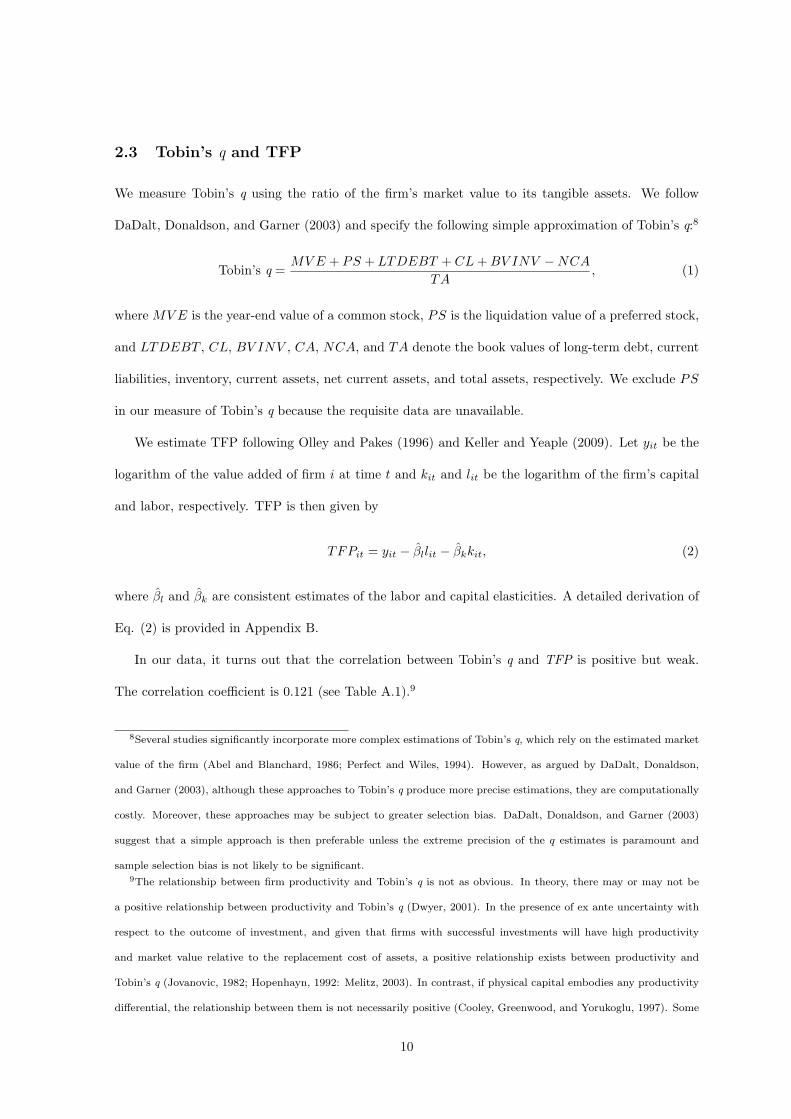
2.3 Tobin’s q and TFP
We measure Tobin’s q using the ratio of the firm’s market value to its tangible assets. We follow
DaDalt, Donaldson, and Garner (2003) and specify the following simple approximation of Tobin’s q:8
Tobin’s q =MVE + PS + LTDEBT + CL+BV INV −NCA
TA, (1)
where MVE is the year-end value of a common stock, PS is the liquidation value of a preferred stock,
and LTDEBT , CL, BV INV , CA, NCA, and TA denote the book values of long-term debt, current
liabilities, inventory, current assets, net current assets, and total assets, respectively. We exclude PS
in our measure of Tobin’s q because the requisite data are unavailable.
We estimate TFP following Olley and Pakes (1996) and Keller and Yeaple (2009). Let yit be the
logarithm of the value added of firm i at time t and kit and lit be the logarithm of the firm’s capital
and labor, respectively. TFP is then given by
TFPit = yit − βllit − βkkit, (2)
where βl and βk are consistent estimates of the labor and capital elasticities. A detailed derivation of
Eq. (2) is provided in Appendix B.
In our data, it turns out that the correlation between Tobin’s q and TFP is positive but weak.
The correlation coefficient is 0.121 (see Table A.1).9
8Several studies significantly incorporate more complex estimations of Tobin’s q, which rely on the estimated market
value of the firm (Abel and Blanchard, 1986; Perfect and Wiles, 1994). However, as argued by DaDalt, Donaldson,
and Garner (2003), although these approaches to Tobin’s q produce more precise estimations, they are computationally
costly. Moreover, these approaches may be subject to greater selection bias. DaDalt, Donaldson, and Garner (2003)
suggest that a simple approach is then preferable unless the extreme precision of the q estimates is paramount and
sample selection bias is not likely to be significant.9The relationship between firm productivity and Tobin’s q is not as obvious. In theory, there may or may not be
a positive relationship between productivity and Tobin’s q (Dwyer, 2001). In the presence of ex ante uncertainty with
respect to the outcome of investment, and given that firms with successful investments will have high productivity
and market value relative to the replacement cost of assets, a positive relationship exists between productivity and
Tobin’s q (Jovanovic, 1982; Hopenhayn, 1992: Melitz, 2003). In contrast, if physical capital embodies any productivity
differential, the relationship between them is not necessarily positive (Cooley, Greenwood, and Yorukoglu, 1997). Some
10
3 Estimation Strategy
Our primary estimation strategy is to employ quantile regression (QR). As discussed in the previous
section, the globalization indexes in our sample have a strong negatively skewed distribution, indicat-
ing that heterogeneity across firms may be substantial. Thus, relationships between the globalization
indexes and firm characteristics also may differ across firms. The major advantage of quantile regres-
sion is that it can provide information about the relationship at different points in the conditional
distribution of the globalization indexes. In contrast, traditional regression techniques, such as or-
dinary least squares (OLS), can only summarize the average relationship between the globalization
indexes and the set of regressors. A key underlying assumption of such traditional techniques is that
the effects of the regressors on the dependent variable are best represented at the conditional mean of
the dependent variable. This is not the case in the presence of a skewed distribution.
In our analysis, we first use an algorithm known as least absolute deviations (LAD) to provide
quantile estimates, where the estimation is implemented by solving linear programming problems.10
We then address endogeneity. Endogeneity potentially arises because factors that simultaneously
influence the choice of globalization mode and Tobin’s q or TFP may exist. The problems of omitted
variables or sample selection also may involve endogeneity. To control for possible endogeneity, we
employ the endogenous quantile regression (QRIV) technique proposed by Lee (2007). The estimation
procedure consists of two steps. The first step is to estimate the residuals of the reduced-form equation
for the endogenous explanatory variables, i.e., Tobin’s q or TFP. The second step is to estimate the
primary equation, which describes the relation between the choice of globalization mode and Tobin’s
q or TFP, using the reduced-form residual as an additional explanatory variable.
In general, it is not easy to find appropriate instrumental variables (IVs). We employ IVs that are
assumed to be correlated with factors that determine the firm performance, suggested by Griliches
(1981) and others. We use two sets of IVs to check the robustness of our estimation results. The
first set includes the logarithm of sales LnS, the ratio of profits to the equipment capital PK, and
studies in the corporate finance literature find a positive relationship between firm productivity and Tobin’s q even after
controlling other factors that affect the firm’s market value (Palia and Lichtenberg, 1999; Dwyer, 2001).10See Cameron and Trivedi (2009) for the detailed Stata command for the QR.
11
the logarithm of the years in business of the headquarters company LnTB . LnS and LnTB are used
as proxy variables for firm size and business experience, respectively. We denote the QRIV with the
first set of IVs as QRIV(1). The second set of IVs consists of LnKL and LnRL, which respectively
denote the ratio of the equipment capital to labor input and the ratio of R&D stock to labor input (in
logs) for the headquarters company, such that LnKL = ln(K/L) and LnRL = ln(RD/L). LnKL and
LnRL measure the physical capital intensity and the R&D intensity of the headquarters company,
respectively. Appendix A provides details on the calculation of the equipment capital (K) and the
R&D stock (RD). We measure labor input (L) using the number of full-time employees. We denote
the QRIV with the second set of IVs as QRIV(2). We assume that if changes in these IVs are not
controlled, they will be part of the error, accounting for inconsistent estimates as long as they are
correlated with the performance of the headquarters companies, such as Tobin’s q and TFP.11
4 Empirical Results
In this section, we report our estimation results. We first analyze the effects of Tobin’s q and TFP
on the degree of firm engagement in a particular globalization mode by regressing each of RXD,
RID, RIhD, and ROD on Tobin’s q and TFP. As reported in the supplementary appendix, our
estimation results indicate that the coefficients are generally significantly positive at high quantiles
for both Tobin’s q and TFP, which suggests that Tobin’s q and TFP are both positively related to
engagement in globalization activity. Thus, our results concur with existing theoretical and empirical
findings. See the supplement for details of these results.
We next regress the indexes of the relative choice of globalization mode on Tobin’s q and TFP. As
we calculate the ratios of the two globalization modes (i.e., exports to horizontal FDI for RXIh and
foreign outsourcing to the total FDI for ROI), we exclude the observations that have zero values for
at least one of the two modes. We report our regression results for Tobin’s q and TFP separately in
the following subsections.
11Table A.1 reports the correlations of the variables. As shown in this table, our IVs are fairly correlated with either
or both of Tobin’s q and TFP , while they have no evident correlation with the indexes of globalization activity.
12
4.1 The effects of Tobin’s q
We first report our estimation results regarding the effects of Tobin’s q on the relative choice of
globalization modes. The upper panel of Table 3 summarizes the results from the OLS, robust OLS
(ROLS), and QR estimations of RXIh and ROI on the logarithm of Tobin’s q, denoted LnQ.12 The
OLS estimates shown in the first column yield an insignificant coefficient of LnQ for both RXIh
and ROI, and the magnitude of the estimated coefficients is relatively large, suggesting that the
presence of outliers seriously affects the regression coefficients. ROLS is an estimation technique that
can address the issue of outliers. We employ ROLS with two types of weights—Huber weighting and
biweighting.13 As reported in the second column, the magnitude of the estimated coefficients becomes
modest by employing ROLS. Although negatively significant estimates are obtained for both RXIh
and ROI, they are highly sensitive to the choice of the biweight tuning constant.
Columns 3–7 report the results from the QR estimations. As shown in the table, we apply QR at
five quantiles: 0.10, 0.25, 0.50, 0.75, and 0.90. The results indicate that the point estimates and the
statistical significance of the estimated coefficients from QR differ substantially across the quantiles
and from the OLS or ROLS estimates. The estimated coefficient of LnQ in the regression of RXIh
is statistically insignificant, except for the point estimate at the 0.90 quantile, which is significantly
positive. In the regression of ROI, in contrast, the coefficient of LnQ is significantly negative at the
0.10, 0.50, 0.75, and 0.90 quantiles, and its significance level reaches 10.5% at the 0.25 quantile. Thus,
an increase in Tobin’s q tends to motivate a firm toward more FDI and away from foreign outsourcing.
(Insert Table 3 around here.)
To check the robustness of the QR findings, and to account for the possible endogeneity of both
TFP and Tobin’s q, we employ a QRIV technique using two sets of IVs, as explained in the previous
section. Table 4 reports the estimated coefficients of LnQ from QRIV.14 Similar to the estimations in
12The estimations of QR are implemented using Stata’s command sqreg with 500 bootstrapping replications.13The ROLS estimations are implemented using Stata’s command rreg. It first runs the OLS and obtains the Cook’s
distance for each observation. Then, after dropping observations with Cook’s distance greater than one, the iteration
process begins with calculating weights based on absolute residuals. See Huber (1981) for details on robust regressions.14The estimation is implemented using Stata’s command cqiv. The Stata code for cqiv is released and introduced
13
Table 3, we apply QRIV at 0.10, 0.25, 0.50, 0.75, and 0.90 quantiles. In this table, the values in square
brackets indicate the lower and upper bounds of a 95% confidence interval. QRIV(1) and QRIV(2)
indicate the estimated results from QRIV with the first and the second sets of IVs, respectively. The
upper panel of Table 4 summarizes the regression of RXIh on LnQ. The coefficients of LnQ are
positively significant at the 0.10 and 0.25 quantiles in QRIV(1) and at the 0.10 quantile in QRIV(2),
and they are insignificant at all other quantiles. The lower panel of Table 4 shows the results of QRIV
estimations for ROI. The estimated coefficients of LnQ are significantly negative at all quantiles
in QRIV(1). In QRIV(2), the coefficients of LnQ are significantly negative at the 0.50 and 0.75
quantiles. Although the significance level at the 0.25 quantile is greater than 12%, the pointwise
confidence interval at the 0.25 quantile does not include zero. These results indicate that the findings
from QR estimation are robust even after controlling for endogeneity and that the two sets of IVs
yield consistent estimates for the most part. That is, LnQ has a significantly negative effect on ROI,
whereas it has no definite effect on RXIh. The former strongly supports the hypothesis of CHM
that firms producing goods with a higher knowledge capital intensity tend to choose FDI over foreign
outsourcing.
(Insert Table 4 around here.)
4.2 The effects of TFP
We turn to the analysis of the effects of TFP. The lower panel of Table 3 summarizes the results from
the OLS, ROLS, and QR estimations of RXIh and ROI on TFP .15 First, the OLS estimate of TFP
shown in the first column is subject to the same problem as that of LnQ. It seems to be seriously
affected by the presence of outliers. Second, as shown in the second column, the ROLS estimates
of TFP indicate the modest magnitude but still insignificant. As in the analysis of Tobin’s q, the
by Chernozhukov, Fernandez-Val, and Kowalski (2011). We employ an endogenous quantile estimation involved in cqiv
without censoring, which is developed on the basis of Lee (2007). The information required to build pointwise confidence
intervals is obtained by 500 bootstrap replications. The value of t-statistics is measured using the bootstrap mean and
the lower and upper bounds of a 95% confidence interval.15See footnotes 12 and 13 for an explanation of QR and ROLS estimations.
14
estimated results from ROLS are highly sensitive to the choice of the biweight tuning constant. Third,
the QR estimates are shown in columns 3–7. The estimated coefficients of TFP in the regression of
RXIh are insignificant at the 0.10 and 0.25 quantiles, and it turns significantly negative with the
11% significance level at the 0.50 quantile. The estimates become significantly negative at the 0.75
and 0.90 quantiles. This result implies that a higher TFP favors horizontal FDI over exports at high
quantiles. In the regression of ROI, on the other hand, the estimated coefficient is insignificant at all
quantiles.
Table 5 reports the estimated coefficients from QRIV.16 As in the analysis of Tobin’s q, we es-
timate QRIV with two sets of IVs. These results are indicated as QRIV(1) and QRIV(2) in Table
5. The upper panel of Table 5 summarizes the regression of RXIh on TFP . In both QRIV(1) and
QRIV(2), the estimated coefficients of TFP are now significantly negative at the 0.50, 0.75, and 0.90
quantiles. These results indicates that controlling for endogeneity strengthens the estimated results.
TFP has a significantly negative effect on RXIh at higher quantiles. It implies that an increase in firm
productivity tends to motivate a firm to choose a greater horizontal FDI and less export, conditional
on the firm engaging in a higher rate of exports relative to horizontal FDI. This result supports the
hypothesis of HMY. The lower panel reports the results from QRIV for ROI. In QRIV(1), we obtain
negative but insignificant estimates for the coefficient of TFP at all quantiles other than the 0.10
quantile. On the other hand, in QRIV(2), TFP yields positive but again insignificant estimates at all
quantiles. Thus, we cannot find any significant effect of TFP on the choice between FDI and foreign
outsourcing.
(Insert Table 5 around here.)
4.3 Graphical presentation of the estimated results
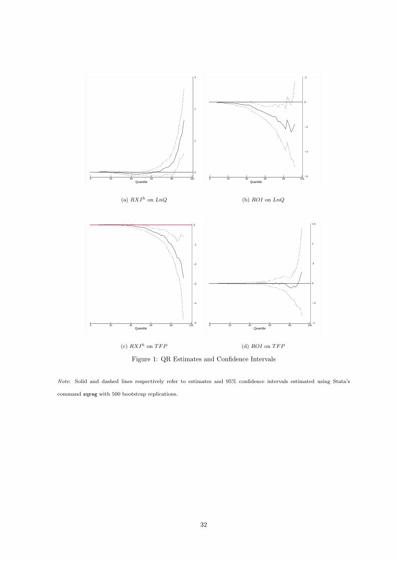
Finally, we plot point and interval estimates from QR in Figure 1 and those from QRIV with two
different sets of IVs in Figures 2 and 3. In each panel in these figures, the horizontal axis measures
the quantile, and the vertical axis measures the value of estimates. Moreover, the thick black lines
16See footnote 14 for an explanation of QRIV estimation.
15
depict the point estimates at various quantiles and dashed lines indicate the lower and upper bounds
of a 95% confidence interval. These figures report the estimated results for all quantiles rather than at
particularly selected quantiles. Figure 1 depicts the estimates for LnQ in panels (a) and (b) and those
for TFP in panels (c) and (d). Panel (a) shows that the 95% confidence interval for the estimate of
RXIh on LnQ crosses zero at most quantiles and lies above zero at the quantiles higher than 0.80.
In the regression of ROI on LnQ (panel (b)), the confidence interval does not include zero at most
quantiles, while there are some disturbances at the quantiles higher than 0.90, which may be due to
the endogeneity problem. In the estimations of RXIh on TFP (panel (c)), the confidence interval
for the estimate crosses zero at lower quantiles and is below zero at higher quantiles. Panel (d) shows
that the confidence interval for the estimate of ROI on TFP includes zero throughout the quantiles.
(Insert Figure 1 around here.)
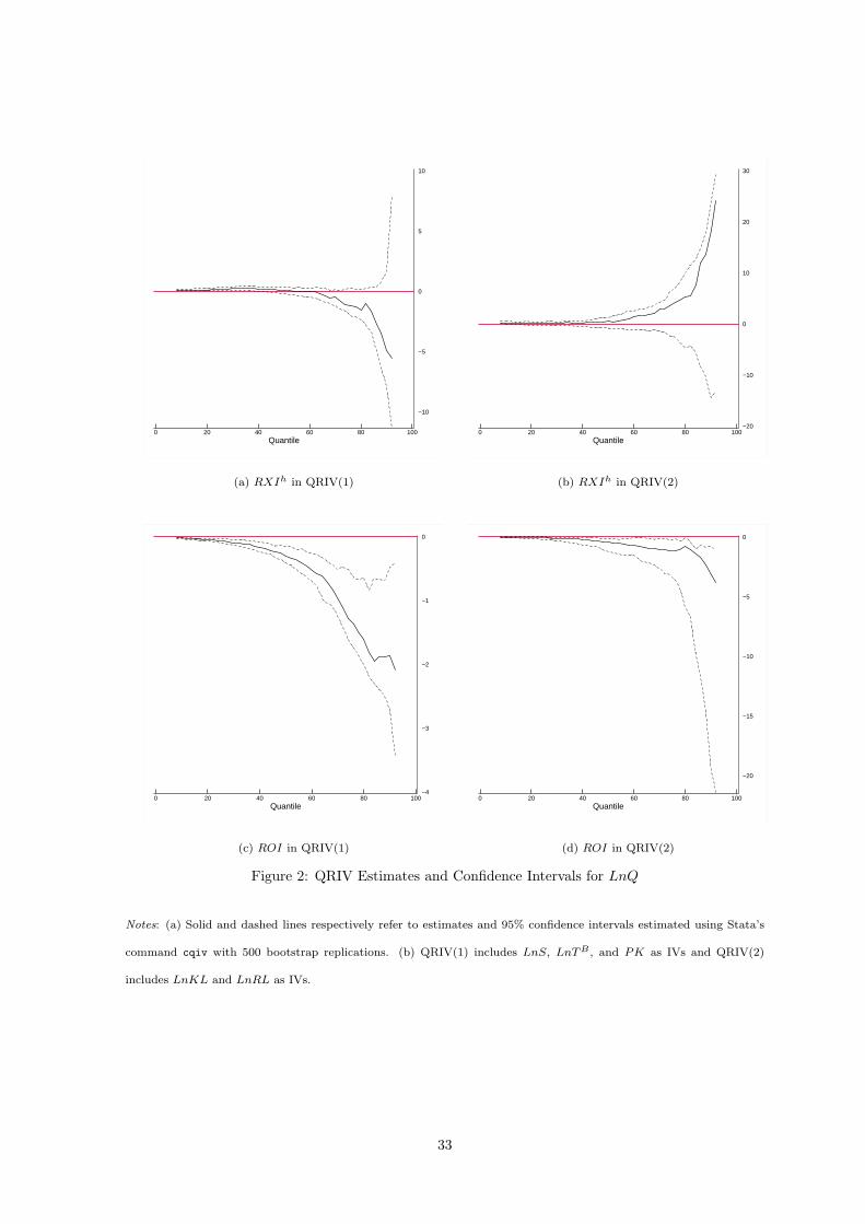
Figures 2 and 3 indicate that the importance of controlling for the endogeneity is apparent and
that the two sets of IVs yield consistent results for the QRIV regressions. Figure 2 reports point
and interval estimates from QRIV for LnQ. Panels (a) and (b) in it show that the 95% confidence
interval in the regression of RXIh on LnQ includes zero at quantiles higher than 0.40 in QRIV(1) and
higher than 0.20 in QRIV(2). In contrast, panels (c) and (d) show that the confidence interval for the
estimated coefficient of LnQ in the regression of ROI lies below zero at all quantiles in QRIV(1) and at
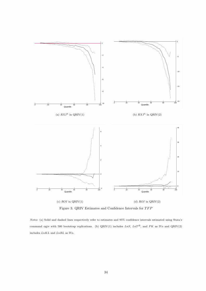
quantiles higher than 0.20 in QRIV(2). Figure 3 reports the QRIV estimates for TFP . Panels (a) and
(b) in it show that the confidence interval in the regression of RXIh is below zero at quantiles higher
than 0.50 in both QRIV(1) and QRIV(2). In panels (c) and (d), on the other hand, the estimates of
ROI on TFP are insignificant at most quantiles.
(Insert Figures 2 and 3 around here.)
5 Conclusion
Using Japanese firm-level data, we empirically investigated how the firm choice of globalization mode
differs according to Tobin’s q and TFP. We found that firms with a higher Tobin’s q tend to choose a
16
greater FDI and less foreign outsourcing, which supports the prediction of CHM. However, we could
not find any definite effect of Tobin’s q on the choice between FDI and exports. On the other hand,
firms with a higher TFP tend to choose a greater FDI and less exports, which supports the prediction
by HMY. However, the choice between FDI and foreign outsourcing is not affected by any difference
in TFP. Controlling for endogeneity with IVs in QR strengthened our estimation results for the most
part. This is the first empirical study that analyzes the relationship between Tobin’s q and the choice
of globalization mode. Moreover, although many previous empirical studies have investigated the
relationship between firm productivity and the choice of exports versus FDI, this paper provided new
evidence that multinationals with a higher TFP favor FDI over exports.
According to our empirical analysis of the links between Tobin’s q and the choice of globalization
mode, the knowledge capital intensity does affect the choice between FDI and foreign outsourcing, as
CHM demonstrate. However, the knowledge capital intensity is not so important when a firm makes a
choice between exports and FDI. This may be because domestic production for exports and the offshore
production under FDI are both undertaken within the boundary of the firm. On the other hand, our
analysis also demonstrates that the ordering of firm productivity may not be monotonically related to
the choice between FDI and foreign outsourcing. This finding may appear to be inconsistent with the
prediction of Antras and Helpman (2004). However, as Grossman, Helpman, and Szeidel (2005) and
Defever and Toubal (2007) show, the productivity ordering in the Antras and Helpman’s (2004) model
depends crucially on the relative size of fixed costs associated to FDI and foreign outsourcing. Thus,
their prediction concerning the productivity ordering is not robust. Our estimates reveal that there
is actually no robust relationship between TFP and the choice of FDI versus foreign outsourcing.
Finally, our results suggest that QR is an appropriate estimation technique when analyzing the
relationship between the globalization mode and firm characteristics because the distributions of the
indexes of globalization activities have strong negative skewness and include outliers. Results obtained
from employing traditional estimation techniques that yield information only at the conditional mean
of the dependent variable may be unsatisfactory. QR provides more valuable information on the effects
of the regressors than such traditional techniques. Actually, our QR estimations revealed that the
17

effects of Tobin’s q or TFP on the choice of the globalization mode could vary among quantiles.
18
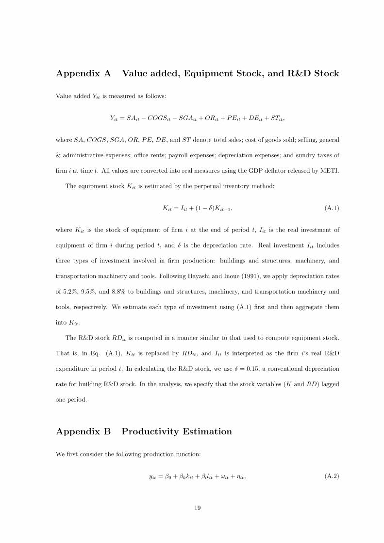
Appendix A Value added, Equipment Stock, and R&D Stock
Value added Yit is measured as follows:
Yit = SAit − COGSit − SGAit +ORit + PEit +DEit + STit,
where SA, COGS, SGA, OR, PE, DE, and ST denote total sales; cost of goods sold; selling, general
& administrative expenses; office rents; payroll expenses; depreciation expenses; and sundry taxes of
firm i at time t. All values are converted into real measures using the GDP deflator released by METI.
The equipment stock Kit is estimated by the perpetual inventory method:
Kit = Iit + (1− δ)Kit−1, (A.1)
where Kit is the stock of equipment of firm i at the end of period t, Iit is the real investment of
equipment of firm i during period t, and δ is the depreciation rate. Real investment Iit includes
three types of investment involved in firm production: buildings and structures, machinery, and
transportation machinery and tools. Following Hayashi and Inoue (1991), we apply depreciation rates
of 5.2%, 9.5%, and 8.8% to buildings and structures, machinery, and transportation machinery and
tools, respectively. We estimate each type of investment using (A.1) first and then aggregate them
into Kit.
The R&D stock RDit is computed in a manner similar to that used to compute equipment stock.
That is, in Eq. (A.1), Kit is replaced by RDit, and Iit is interpreted as the firm i’s real R&D
expenditure in period t. In calculating the R&D stock, we use δ = 0.15, a conventional depreciation
rate for building R&D stock. In the analysis, we specify that the stock variables (K and RD) lagged
one period.
Appendix B Productivity Estimation
We first consider the following production function:
yit = β0 + βkkit + βllit + ωit + ηit, (A.2)
19
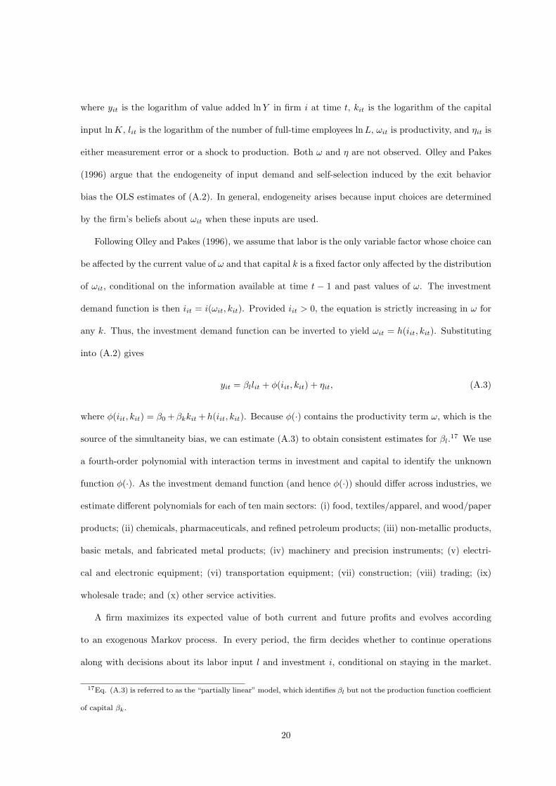
where yit is the logarithm of value added lnY in firm i at time t, kit is the logarithm of the capital
input lnK, lit is the logarithm of the number of full-time employees lnL, ωit is productivity, and ηit is
either measurement error or a shock to production. Both ω and η are not observed. Olley and Pakes
(1996) argue that the endogeneity of input demand and self-selection induced by the exit behavior
bias the OLS estimates of (A.2). In general, endogeneity arises because input choices are determined
by the firm’s beliefs about ωit when these inputs are used.
Following Olley and Pakes (1996), we assume that labor is the only variable factor whose choice can
be affected by the current value of ω and that capital k is a fixed factor only affected by the distribution
of ωit, conditional on the information available at time t − 1 and past values of ω. The investment
demand function is then iit = i(ωit, kit). Provided iit > 0, the equation is strictly increasing in ω for
any k. Thus, the investment demand function can be inverted to yield ωit = h(iit, kit). Substituting
into (A.2) gives
yit = βllit + ϕ(iit, kit) + ηit, (A.3)
where ϕ(iit, kit) = β0 +βkkit +h(iit, kit). Because ϕ(·) contains the productivity term ω, which is the
source of the simultaneity bias, we can estimate (A.3) to obtain consistent estimates for βl.17 We use
a fourth-order polynomial with interaction terms in investment and capital to identify the unknown
function ϕ(·). As the investment demand function (and hence ϕ(·)) should differ across industries, we
estimate different polynomials for each of ten main sectors: (i) food, textiles/apparel, and wood/paper
products; (ii) chemicals, pharmaceuticals, and refined petroleum products; (iii) non-metallic products,
basic metals, and fabricated metal products; (iv) machinery and precision instruments; (v) electri-
cal and electronic equipment; (vi) transportation equipment; (vii) construction; (viii) trading; (ix)
wholesale trade; and (x) other service activities.
A firm maximizes its expected value of both current and future profits and evolves according
to an exogenous Markov process. In every period, the firm decides whether to continue operations
along with decisions about its labor input l and investment i, conditional on staying in the market.
17Eq. (A.3) is referred to as the “partially linear” model, which identifies βl but not the production function coefficient
of capital βk.
20
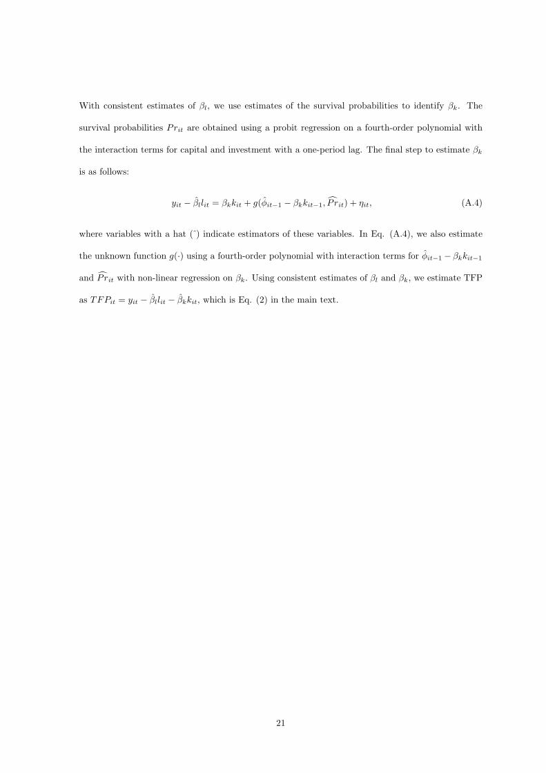
With consistent estimates of βl, we use estimates of the survival probabilities to identify βk. The
survival probabilities Prit are obtained using a probit regression on a fourth-order polynomial with
the interaction terms for capital and investment with a one-period lag. The final step to estimate βk
is as follows:
yit − βllit = βkkit + g(ϕit−1 − βkkit−1, P rit) + ηit, (A.4)
where variables with a hat ( ) indicate estimators of these variables. In Eq. (A.4), we also estimate
the unknown function g(·) using a fourth-order polynomial with interaction terms for ϕit−1 − βkkit−1
and P rit with non-linear regression on βk. Using consistent estimates of βl and βk, we estimate TFP
as TFPit = yit − βllit − βkkit, which is Eq. (2) in the main text.
21
REFERENCES
Abel, Andrew B. and Oliver J. Blanchard, “The present value of profits and cyclical movements in
investment,” Econometrica 54:2 (1986), 249–73.
Antras, Pol and Elhanan Helpman, “Global sourcing,” Journal of Political Economy 112:3 (2004),
552–80.
Bernard, Andrew B. and J. Bradford Jensen, “Exporters, jobs, and wages in U.S. manufacturing:
1976–87,” Brookings Papers on Economic Activity, Microeconomics 1995 (1995), 67–112.
Bernard, Andrew B. and J. Bradford Jensen, “Exceptional exporter performance: Cause, effect, or
both?” Journal of International Economics 47:1 (1999), 1–25.
Cameron, A. Colin and Pravin K. Trivedi, Microeconometrics: Using Stata. (College Station, TX:
STATA Press, 2009).
Chen, Yongmin, Ignatius J. Horstmann, and James R. Markusen, “Physical capital, knowledge
capital, and the choice between FDI and outsourcing,” Canadian Journal of Economics 45:1
(2012), 1–15.
Chernozhukov, Victor, Ivan Fernandez-Val, and Amanda Kowalski, “Quantile regression with cen-
soring and endogeneity,” NBER working paper no. 16997 (2011).
Cooley, Thomas F., Jeremy Greenwood, and Mehmet Yorukoglu, “The replacement problem,” Jour-
nal of Monetary Economics 40:3 (1997), 457–99.
DaDalt, Peter J., Jeffrey R. Donaldson, and Jacqueline L. Garner, “Will any q do?” Journal of
Financial Research 26:4 (2003), 535–51.
Defever, Fabrice and Farid Toubal, “Productivity and the sourcing modes of multinational firms:
Evidence from French firm-level data,” CEP discussion paper no. 842 (2007).
Dwyer, Douglas W., “Plant-level productivity and the market value of a firm,” Center for Economic
Research, U.S. Census Bureau working paper 01–03 (2001).
22
Federico, Stefano, “Outsourcing versus integration at home or abroad and firm heterogeneity,” Em-
pirica 37:1 (2010), 47–63.
Greenaway, David and Richard Kneller, “Firm heterogeneity, exporting and foreign direct invest-
ment,” Economic Journal 117:517 (2007), F134–61.
Griliches, Zvi, “Market value, R&D, and patents,” Economic Letters 7:2 (1981), 183–7.
Grossman, Gene M., Elhanan Helpman, and Adam Szeidl, “Complementarities between outsourcing
and foreign sourcing,” American Economic Review 95:2 (2005), 19–24.
Grossman, Sanford J. and Oliver D. Hart, “The costs and benefits of ownership: A theory of vertical
and lateral integration,” Journal of Political Economy 94:4 (1986), 691–719.
Hart, Oliver and John Moore, “Property rights and the nature of the firm,” Journal of Political
Economy 98:6 (1990), 1119–58.
Hayashi, Fumio and Tohru Inoue, “The relation between firm growth and Q with multiple capital
goods: Theory and evidence from panel data on Japanese firms,” Econometrica 59:3 (1991),
731–53.
Head, Keith and John Ries, “Heterogeneity and the FDI versus export decision of Japanese manu-
facturers,” Journal of the Japanese and International Economies 17:4 (2003), 448–67.
Helpman, Elhanan, “Trade, FDI, and the organization of firms,” Journal of Economic Literature
44:3 (2006), 589–630.
Helpman, Elhanan, Marc J. Melitz, and Stephen R. Yeaple, “Export versus FDI with heterogeneous
firms,” American Economic Review 94:1 (2004), 300–16.
Hopenhayn, Hugo A., “Entry, exit, and firm dynamics in long run equilibrium,” Econometrica 60:5
(1992), 1127–50.
Horstmann, Ignatius J. and James R. Markusen, “Licensing versus direct investment: A model of
internalization by the multinational enterprise,” Canadian Journal of Economics 20:3 (1987),
464–81.
23
Huber, Peter J., Robust Statistics (New York: John Wiley and Sons, 1981).
Jovanovic, Boyan, “Selection and the evolution of industry,” Econometrica 50:3 (1982), 649–70.
Keller, Wolfgang and Stephen R. Yeaple, “Multinational enterprises, international trade, and produc-
tivity growth: Firm-level evidence from the United States.” this REVIEW 91:4 (2009), 821–31.
Kimura, Fukunari and Kozo Kiyota, “Exports, FDI, and productivity: Dynamic evidence from
Japanese firms,” Review of World Economics 142:2 (2006), 695–719.
Koenker, Roger, Quantile Regression (Cambridge: Cambridge University Press, 2005).
Koenker, Roger and Gilbert Bassett, “Regression quantiles,” Econometrica 46:1 (1978), 33–50.
Koenker, Roger and Kevin F. Hallock, “Quantile regression,” Journal of Economic Perspectives 15:4
(2001), 143–56.
Kohler, Wilhelm K. and Marcel Smolka, “Global sourcing decisions and firm productivity: Evi-
dence from Spain,” In R.M. Stern (Ed.), Quantitative Analysis of Newly Evolving Patterns of
International Trade: Fragmentation, Offshoring of Activities, and Vertical Intra-Industry Trade.
(Hackensack: World Scientific, 2012).
Lee, Sokbae, “Endogeneity in quantile regression models: A control function approach,” Journal of
Econometrics 141:2 (2007), 1131–58.
Markusen, James R., “Multinationals, multi-plant economies, and the gains from trade,” Journal of
International Economics 16:3–4 (1984), 205–26.
Markusen, James R., Multinational Firms and the Theory of International Trade (Cambridge: MIT
Press, 2002).
Mayer, Thierry and Gianmarco I.P. Ottaviano, The Happy Few: The Internationalisation of Euro-
pean Firms. Bruegel Blueprint Series (2007).
Melitz, Marc J., “The impact of trade on intra-industry reallocations and aggregate industry pro-
ductivity,” Econometrica 71:6 (2003), 1695–725.
24
Olley, G. Steven and Ariel Pakes, “The dynamics of productivity in the telecommunications equip-
ment industry,” Econometrica 64:6 (1996), 1263–97.
Palia, Darius and Frank Lichtenberg, “Managerial ownership and firm performance: A re-
examination using productivity measurement,” Journal of Corporate Finance 5:4 (1999), 323–
339.
Perfect, Steven B. and Kenneth W. Wiles, “Alternative construction of Tobin’s q: An empirical
comparison,” Journal of Empirical Finance 1:3–4 (1994), 313–41.
Tomiura, Eiichi, “Foreign outsourcing, exporting, and FDI: A productivity comparison at the firm
level,” Journal of International Economics 72:1 (2007), 113–127.
Trofimenko, Natalia, “Learning by exporting: Does it matter where one learns? Evidence from
Colombian manufacturing firms,” Economic Development and Cultural Change 56:4 (2008), 871–
94.
Wagner, Joachim, “Export intensity and plant characteristics: What can we learn from quantile
regression?” Review of World Economics 142:1 (2006), 195–203.
—— “Exports and productivity: A survey of the evidence from firm-level data.” World Economy
30:1 (2007), 60–82.
—— “International trade and firm performance: A survey of empirical studies since 2006,” Review
of World Economics, 148:2 (2012), 235–67.
25
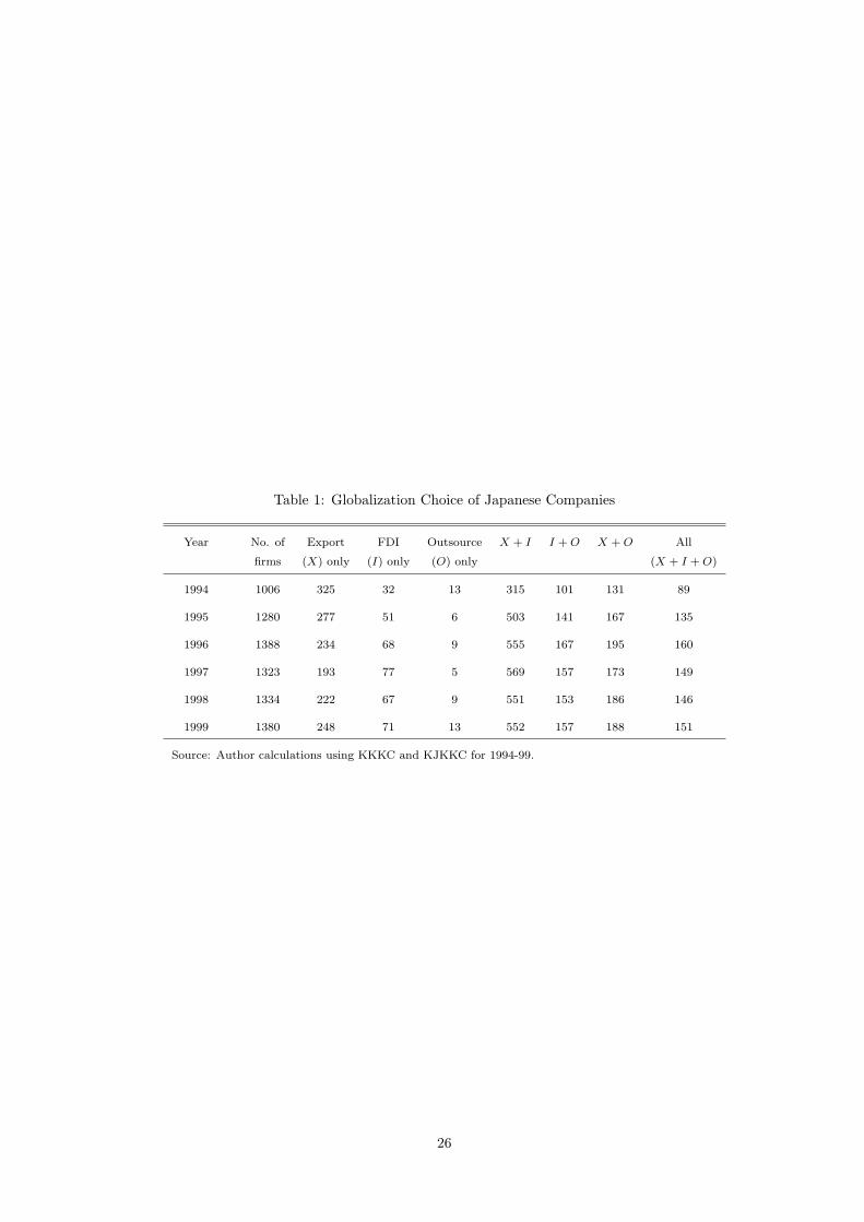
Table 1: Globalization Choice of Japanese Companies
Year No. of Export FDI Outsource X + I I +O X +O All
firms (X) only (I) only (O) only (X + I +O)
1994 1006 325 32 13 315 101 131 89
1995 1280 277 51 6 503 141 167 135
1996 1388 234 68 9 555 167 195 160
1997 1323 193 77 5 569 157 173 149
1998 1334 222 67 9 551 153 186 146
1999 1380 248 71 13 552 157 188 151
Source: Author calculations using KKKC and KJKKC for 1994-99.
26
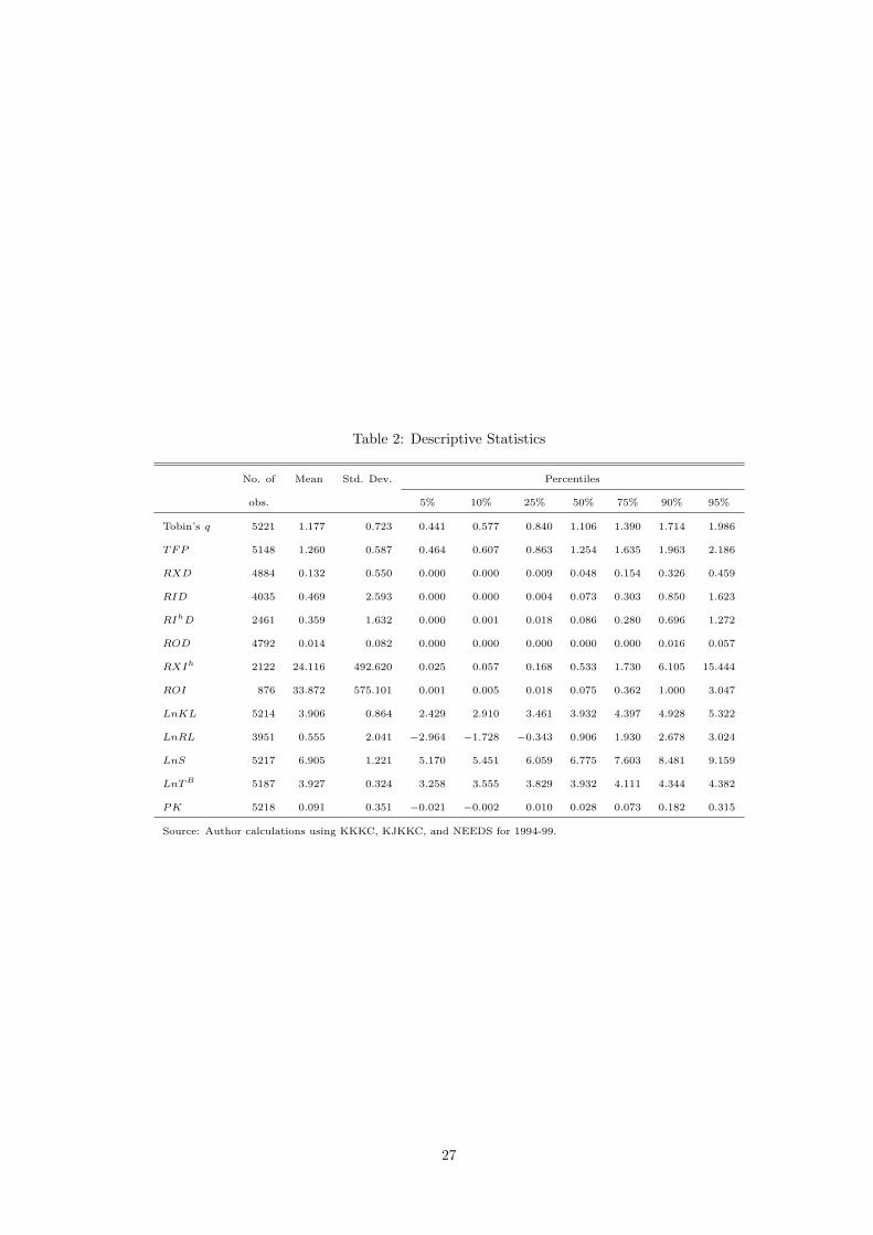
Table 2: Descriptive Statistics
No. of Mean Std. Dev. Percentiles
obs. 5% 10% 25% 50% 75% 90% 95%
Tobin’s q 5221 1.177 0.723 0.441 0.577 0.840 1.106 1.390 1.714 1.986
TFP 5148 1.260 0.587 0.464 0.607 0.863 1.254 1.635 1.963 2.186
RXD 4884 0.132 0.550 0.000 0.000 0.009 0.048 0.154 0.326 0.459
RID 4035 0.469 2.593 0.000 0.000 0.004 0.073 0.303 0.850 1.623
RIhD 2461 0.359 1.632 0.000 0.001 0.018 0.086 0.280 0.696 1.272
ROD 4792 0.014 0.082 0.000 0.000 0.000 0.000 0.000 0.016 0.057
RXIh 2122 24.116 492.620 0.025 0.057 0.168 0.533 1.730 6.105 15.444
ROI 876 33.872 575.101 0.001 0.005 0.018 0.075 0.362 1.000 3.047
LnKL 5214 3.906 0.864 2.429 2.910 3.461 3.932 4.397 4.928 5.322
LnRL 3951 0.555 2.041 −2.964 −1.728 −0.343 0.906 1.930 2.678 3.024
LnS 5217 6.905 1.221 5.170 5.451 6.059 6.775 7.603 8.481 9.159
LnTB 5187 3.927 0.324 3.258 3.555 3.829 3.932 4.111 4.344 4.382
PK 5218 0.091 0.351 −0.021 −0.002 0.010 0.028 0.073 0.182 0.315
Source: Author calculations using KKKC, KJKKC, and NEEDS for 1994-99.
27
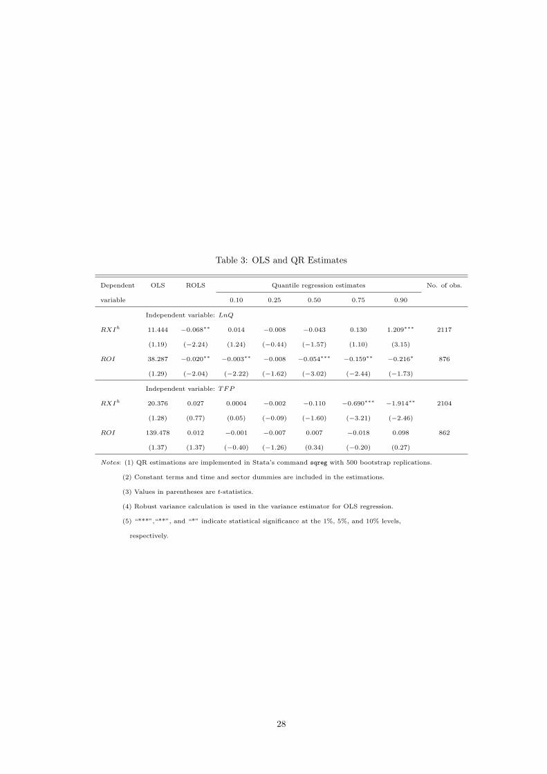
Table 3: OLS and QR Estimates
Dependent OLS ROLS Quantile regression estimates No. of obs.
variable 0.10 0.25 0.50 0.75 0.90
Independent variable: LnQ
RXIh 11.444 −0.068∗∗ 0.014 −0.008 −0.043 0.130 1.209∗∗∗ 2117
(1.19) (−2.24) (1.24) (−0.44) (−1.57) (1.10) (3.15)
ROI 38.287 −0.020∗∗ −0.003∗∗ −0.008 −0.054∗∗∗ −0.159∗∗ −0.216∗ 876
(1.29) (−2.04) (−2.22) (−1.62) (−3.02) (−2.44) (−1.73)
Independent variable: TFP
RXIh 20.376 0.027 0.0004 −0.002 −0.110 −0.690∗∗∗ −1.914∗∗ 2104
(1.28) (0.77) (0.05) (−0.09) (−1.60) (−3.21) (−2.46)
ROI 139.478 0.012 −0.001 −0.007 0.007 −0.018 0.098 862
(1.37) (1.37) (−0.40) (−1.26) (0.34) (−0.20) (0.27)
Notes: (1) QR estimations are implemented in Stata’s command sqreg with 500 bootstrap replications.
(2) Constant terms and time and sector dummies are included in the estimations.
(3) Values in parentheses are t-statistics.
(4) Robust variance calculation is used in the variance estimator for OLS regression.
(5) “***”,“**”, and “*” indicate statistical significance at the 1%, 5%, and 10% levels,
respectively.
28
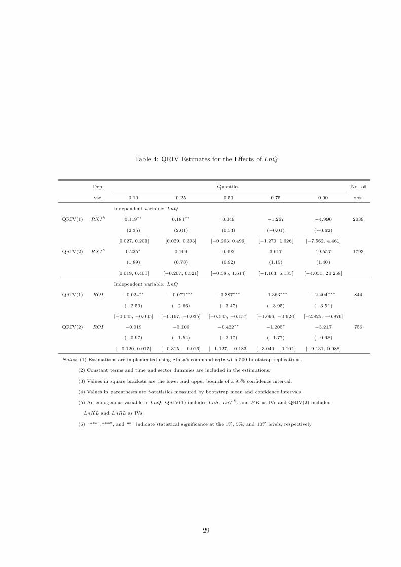
Table 4: QRIV Estimates for the Effects of LnQ
Dep. Quantiles No. of
var. 0.10 0.25 0.50 0.75 0.90 obs.
Independent variable: LnQ
QRIV(1) RXIh 0.119∗∗ 0.181∗∗ 0.049 −1.267 −4.990 2039
(2.35) (2.01) (0.53) (−0.01) (−0.62)
[0.027, 0.201] [0.029, 0.393] [−0.263, 0.496] [−1.270, 1.626] [−7.562, 4.461]
QRIV(2) RXIh 0.225∗ 0.109 0.492 3.617 19.557 1793
(1.89) (0.78) (0.92) (1.15) (1.40)
[0.019, 0.403] [−0.207, 0.521] [−0.385, 1.614] [−1.163, 5.135] [−4.051, 20.258]
Independent variable: LnQ
QRIV(1) ROI −0.024∗∗ −0.071∗∗∗ −0.387∗∗∗ −1.363∗∗∗ −2.404∗∗∗ 844
(−2.50) (−2.66) (−3.47) (−3.95) (−3.51)
[−0.045, −0.005] [−0.167, −0.035] [−0.545, −0.157] [−1.696, −0.624] [−2.825, −0.876]
QRIV(2) ROI −0.019 −0.106 −0.422∗∗ −1.205∗ −3.217 756
(−0.97) (−1.54) (−2.17) (−1.77) (−0.98)
[−0.120, 0.015] [−0.315, −0.016] [−1.127, −0.183] [−3.040, −0.101] [−9.131, 0.988]
Notes: (1) Estimations are implemented using Stata’s command cqiv with 500 bootstrap replications.
(2) Constant terms and time and sector dummies are included in the estimations.
(3) Values in square brackets are the lower and upper bounds of a 95% confidence interval.
(4) Values in parentheses are t-statistics measured by bootstrap mean and confidence intervals.
(5) An endogenous variable is LnQ. QRIV(1) includes LnS, LnTB , and PK as IVs and QRIV(2) includes
LnKL and LnRL as IVs.
(6) “***”,“**”, and “*” indicate statistical significance at the 1%, 5%, and 10% levels, respectively.
29

Table 5: QRIV Estimates for the Effects of TFP
Dep. Quantiles No. of
var. 0.10 0.25 0.50 0.75 0.90 obs.
Independent variable: TFP
QRIV(1) RXIh 0.020 −0.043 −0.298∗∗ −1.215∗∗ −3.891∗∗ 2029
(0.75) (−0.33) (−2.34) (−2.31) (−2.21)
[−0.033, 0.086] [−0.172, 0.102] [−0.778, −0.066] [−2.927, −0.379] [−7.687, −0.349]
QRIV(2) RXIh 0.004 −0.033 −0.464∗ −2.736∗∗∗ −11.341∗∗∗ 1785
(−0.24) (−0.41) (−1.65) (−3.10) (−2.68)
[−0.101, 0.083] [−0.207, 0.153] [−1.282, 0.028] [−5.927, −1.506] [−16.832, −2.740]
Independent variable: TFP
QRIV(1) ROI −0.014∗∗ −0.048 −0.262 −0.296 −0.466 832
(−2.00) (−1.04) (−1.03) (−0.91) (−0.41)
[−0.043, −0.004] [−0.129, 0.015] [−0.344, 0.056] [−0.460, 0.160] [−0.859, 0.927]
QRIV(2) ROI 0.013 0.051 0.238 0.675 1.371 744
(1.00) (1.29) (0.96) (0.29) (−0.06)
[−0.009, 0.041] [−0.025, 0.125] [−0.155, 0.479] [−1.059, 1.163] [−5.823, 3.105]
Notes: (1) Estimations are implemented using Stata’s command cqiv with 500 bootstrap replications.
(2) Constant terms and time and sector dummies are included in the estimations.
(3) Values in square brackets are the lower and upper bounds of a 95% confidence interval.
(4) Values in parentheses are t-statistics measured by bootstrap mean and confidence intervals.
(5) An endogenous variable is TFP . QRIV(1) includes LnS, LnTB , and PK as IVs and QRIV(2) includes
LnKL and LnRL as IVs.
(6) “***”,“**”, and “*” indicate statistical significance at the 1%, 5%, and 10% levels, respectively.
30
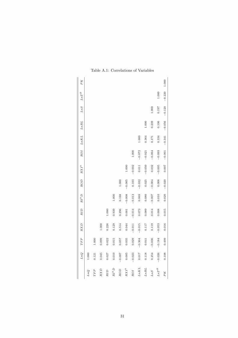
Table A.1: Correlations of Variables
LnQ
TFP
RX
DRID
RIhD
ROD
RX
Ih
ROI
LnK
LLnRL
LnS
LnT
BPK
LnQ
1.000
TFP
0.121
1.000
RX
D0.045
0.099
1.000
RID
0.027
0.022
0.226
1.000
RIhD
0.010
0.015
0.129
0.939
1.000
ROD
−0.007
0.057
0.514
0.296
0.188
1.000
RX
Ih
0.005
0.035
0.044
0.001
−0.008
−0.005
1.000
ROI
−0.023
0.029
−0.011
−0.014
−0.013
0.103
−0.002
1.000
LnK
L0.017
−0.304
−0.015
0.073
0.069
−0.032
0.011
−0.072
1.000
LnRL
0.118
0.041
0.117
0.089
0.080
0.025
−0.050
−0.021
0.364
1.000
LnS
0.254
−0.036
0.119
0.014
−0.007
−0.004
0.032
−0.064
0.171
0.239
1.000
LnT
B−0.026
−0.184
−0.053
0.008
0.010
0.008
−0.005
−0.093
0.334
0.106
0.197
1.000
PK
0.108
0.499
0.016
0.015
0.020
−0.020
0.007
−0.001
−0.341
−0.056
−0.120
−0.220
1.000
31
0
1
2
3
0 20 40 60 80 100Quantile
(a) RXIh on LnQ
−.6
−.4
−.2
0
.2
0 20 40 60 80 100Quantile
(b) ROI on LnQ
−5
−4
−3
−2
−1
0
0 20 40 60 80 100Quantile
(c) RXIh on TFP
−1
−.5
0
.5
1
1.5
0 20 40 60 80 100Quantile
(d) ROI on TFP
Figure 1: QR Estimates and Confidence Intervals
Note: Solid and dashed lines respectively refer to estimates and 95% confidence intervals estimated using Stata’s
command sqreg with 500 bootstrap replications.
32
−10
−5
0
5
10
0 20 40 60 80 100Quantile
(a) RXIh in QRIV(1)
−20
−10
0
10
20
30
0 20 40 60 80 100Quantile
(b) RXIh in QRIV(2)
−4
−3
−2
−1
0
0 20 40 60 80 100Quantile
(c) ROI in QRIV(1)
−20
−15
−10
−5
0
0 20 40 60 80 100Quantile
(d) ROI in QRIV(2)
Figure 2: QRIV Estimates and Confidence Intervals for LnQ
Notes: (a) Solid and dashed lines respectively refer to estimates and 95% confidence intervals estimated using Stata’s
command cqiv with 500 bootstrap replications. (b) QRIV(1) includes LnS, LnTB , and PK as IVs and QRIV(2)
includes LnKL and LnRL as IVs.
33
−10
−8
−6
−4
−2
0
0 20 40 60 80 100Quantile
(a) RXIh in QRIV(1)
−20
−15
−10
−5
0
0 20 40 60 80 100Quantile
(b) RXIh in QRIV(2)
−2
0
2
4
6
0 20 40 60 80 100Quantile
(c) ROI in QRIV(1)
0
10
20
30
40
0 20 40 60 80 100Quantile
(d) ROI in QRIV(2)
Figure 3: QRIV Estimates and Confidence Intervals for TFP
Notes: (a) Solid and dashed lines respectively refer to estimates and 95% confidence intervals estimated using Stata’s
command cqiv with 500 bootstrap replications. (b) QRIV(1) includes LnS, LnTB , and PK as IVs and QRIV(2)
includes LnKL and LnRL as IVs.
34