ELD ANN MLP

7/21/2019 ELD ANN MLP

http://slidepdf.com/reader/full/eld-ann-mlp 1/5

MLP’s Predictive Models to Forecast

Electricity Consumption

James Foot* Valeriu Mihai**

*Faculty of Science and Technology, University of the Algarve (e-mail: [email protected]).

** Faculty of Science and Technology, University of the Algarve (e-mail: [email protected]).

Abstract: In this paper, we present a different approach for a short-term prediction of the electricity load

demand (ELD) for the Portuguese power grid. Mainly, we apply a Multilayer perceptron (MLP) artificial

neural network (ANN) to forecast the ELD in a one-step-ahead fashion or every 15 minutes based on

historical (altered) data from the Portuguese power grid company Redes Electricas Nacionais (REN). Indesigning an ANN-MLP for time series forecasting, the variables that are depended to develop the model

process include the number of input, hidden and output neurons are important. There are no specific ways

to determine these parameters, but through the iteration process. To obtain the best performance in

prediction, ANN models require an experimental approach to analyse the ANN design space and

application of different training strategies. The NN models are trained by the Levenberg-Marquardt

algorithm. Different experiments were carried out to show which parameters are crucial to have good

prediction accuracy using non-linear autoregressive predictive model (NAR).

Keywords: Electricity load demand; Power grid; Multilayer perceptron; Artificial Neural Network;

Prediction; Forecast; Modeling; Non-linear autoregressive predictive model.

1. INTRODUCTION

The electricity load demand forecasting is an important

aspect for any modern energy company, with respect to theirsystem management. Load forecasting can be used for

scheduling maintenance, reducing spinning reserve capacity,

scheduling individual plant production, which will improve

the reliability of the grid and reduce cost for the company and

the end consumer. There are several different kinds of

forecast lengths depending on the objectives:

1. Long-term - typically a long-term is a forecast from 1 to

10 years. This is used for major planning and investment,

i.e., if the ELD increases significantly the planning

construction of a new power plant could take up to

several years.

2.

Medium-term - typically a medium-term forecast is froma couple of months to a year. This is used to ensure that

capacity constraints are met in the medium term.

3.

Short-term - typically a short-term forecast is from a few

minutes up to a day. This is used to assist planning and

to manage electricity production.

In this paper we’ll focus on the short-term prediction in order

to better manage the electricity production for the grid. This

project is based on a paper (Ferreira et al., 2010) were the

authors, using Radial Basis Functions ANN, worked on

creating a model to forecast, within a period of 24 to 48

hours, the ELD for the REN .

We were provided with a file eld180dias.txt containing the

values for the ELD that were measured every 15 minutes

during a period of 180 days.

1.1

Characteristics of ELD

There are several variables like time and random effects that

can affect the normal variation of the ELD, a so make it

harder to do a short-term prediction. As you can imagine the

electricity load demand differs from the day to the night, the

demand from the weekend is different from the demand

during the weekdays, but all theses differences have a cyclic

nature, i.e., the ELD at 12 pm on Tuesday should be similar

to the ELD from the previous Tuesday at 12 pm and so on,

although the occurrence of a public holiday or the shift to and

from daylight saving time and even the start of a school year

can cause changes to these cycles. Random effects are

another source of disturbance to the regular ELD; anything

like heavy machinery in a factory being used, widespread

strikes, and special events can affect the load. Since we’ve

only been give data for the ELD values, we can’t consider

any of these variables mentioned above.

The paper is organized as follows: in section 2 we have a

slight overview of the Multilayer perceptron’s (MLP’s) and

the Levenberg-Marquardt algorithm, after that in section 3 we

describe the Data set, in section 4 we talk about the

experiments and the procedure to create and train the

network, in section 5 we show the result and analyse them in

section 6. In section 6 we also talk about future work.



2. MODEL IDENTIFICATION PROCEDURE

As previously mentioned, the data available for this project is

a series of historical measurements; limiting us on the type of

model structure available. A Non-linear Auto-Regressive

(NAR) structure is when the inputs are a series of delay from

the output, i.e., if y is the output of the ANN then:

!

! ! !! ! !! ! ! !! ! ! !!! ! ! ! !!

where, n is the number of delay. The ANN model is trained

by the Levenberg-Marquardt (LM) algorithm.

2.1 Multilayer Perceptron

MLP is a subset of ANN, defined as a system of massively

distributed parallel processors (consisting of simple

processing units called neurons) that have natural tendency

for storing and utilizing experiential knowledge (Yassin,

2009). Generally, the MLP learns the relationship between a

set of inputs and outputs by updating internalinterconnections called weights using the back-propagation

algorithm.

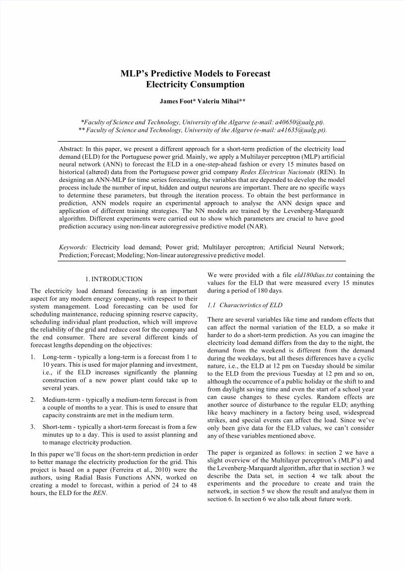
In MLP, the units are arranged in interconnected layers: one

input layer, one (or more) hidden layers, and one output

layer; this can be seen in the figure below. The numbers of

input and output units are typically fixed, since they depend

on the input and desired output(s). However, the training

algorithm and the number of hidden units are adjustable, and

can be set so that it maximizes the performance of the MLP.

Fig. 1. Configuration of a multilayer perceptron. The hidden

component can have more than one layer.

A common problem in MLP training is over-generalization,referring to a condition where the MLP has been trained until

it has memorized the data it’s given, rendering it unable to

adapt and generalize to new cases.

In order to obtain the optimum MLP generalization, the Early

Stopping (ES) method divides the dataset into three sets – the

training set, and independent validation and testing sets. The

training set is used to update the MLP weights during the

training phase, and the error in the independent validation set

is monitored. Since the validation set does not participate in

the training process, it can be used as a performance gauge to

measure the generalization capabilities of the ANN when it

encounters previously untrained cases. If the training errorcontinues to decrease, but the validation set error has started

to increase, this indicates that over-generalization has

occurred, thus training is stopped. ES is widely used because

it is simple to implement and understand, and has been

reported to be superior to regularization methods in many

cases.

2.2

Levenberg-Marquardt

Levenberg-Marquardt algorithm, which was independently

developed by Kenneth Levenberg and Donald Marquardt,

provides a numerical solution to the problem of minimizing a

nonlinear function (Yu et al, 1993; Hagan et al, 1994). It is

fast and has stable convergence. In the artificial neural

network field this algorithm is suitable for small- and

medium-sized problems. The Levenberg-Marquardt

algorithm can be presented as:

!!!! ! !! ! !!! !!! ! !"!!!!!!!

where, ! is always positive, called combination coefficient

and ! is the identity matrix.

3. DATA SET

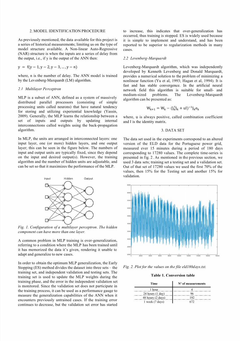
The data set used in the experiments correspond to an altered

version of the ELD data for the Portuguese power grid,

measured ever 15 minutes during a period of 180 days

corresponding to 17280 values. The complete time-series is

presented in fig. 2. As mentioned in the previous section, we

used 3 data sets; training set a testing set and a validation set.

Out of that set of 17280 values we used the first 70% of the

values, then 15% for the Testing set and another 15% for

validation.

Fig. 2. Plot for the values on the file eld180days.txt.

Table 1. Conversion table

Time Nº of measurements

1 hour 4

24 hours (1 day) 96

48 hours (2 days) 1921 week (7 days) 672



Table 2. Data set used in experiments

Data set Training Validation Testing

Percentage (%) 70 15 15

Number of points 12096 2592 2592

Number of days 126 27 27

4. EXPERIMENT

As express in the previous sections there are three parameters

that can be changed in order to improve the: number of

hidden layers, number of neurons in each layer and the

number of delay. With these parameters we conducted three

groups of experiments, in which in each group we altered

only one of the parameters. But before we start the

experiments we need to import the data from a .txt file to a

Matlab column vector in order to be able to pre-process, i.e.,

normalizing them in-between 1 and -1. Next phase was to

decide what would be the values for the different parameters.Our control experiment, experiment A, will have 1 hidden

layer with 4 neurons and ! ! ! delays.

Table 3. Parameters for each experiment

Experiment Parameter Variations

B, C Nº hidden layers 2, 3

D, E, F, G Nº of neurons/layer 8, 16, 32, 64

H ,I, J Nº of delays 6, 9, 96

3.1 Training

After that we want to start training our ANN. To do this weused some functions from the Matlab NN toolbox. First we

create the network using the function narnet (Beale

et.al.,2014) that has inputs for the number of delays, and

hidden layer topology (number of hidden layers and number

of neurons in each layer). Then we use the preparets (Beale

et.al.,2014) function to prepare the values for the training and

simulation. After that we divide the data into the 3 sets

mention earlier, 70% for the training set, 15% for the

validation and 15% for the testing, using the function

divideblock ((Beale et.al.,2014). Next we used the train

(Beale et.al.,2014) function to commence the training of the

ANN. This training function is using the LM algorithm.

3.2 Outputs

The outputs of the training function are a series of plots that

display performance of the ANN that is the MSE per

iteration. The root-mean-square error, that is used measure

the difference between the value predicted by a model and

the values actually observed .The Time-Series Response that

shows the error between the target and the output for each

one of the 3 value sets. The weight values for each of the

connects between the neurons.

At the end all the data is restored to their original values, so

that it makes it easier to understand the results.

5. RESULTS

We ran each experiment 3 times and calculated the average,

in order to improve the reliability of the results.

Table 4. Results for experiment A

Test MSE RMSE Iterations

1 0.00081489 55.078 11

2 0.00077090 53.571 61

3 0.00080887 54.875 5

Average 0.00079822 54.508 26

Table 5. Results for experiment B


1 0.00077030 53.784 34

2 0.00079379 54.361 65

3 0.00080769 54.835 12

Average 0.00079059 54.327 37

Table 6. Results for experiment C


1 0.00078439 54.038 88

2 0.00075733 53.098 430

3 0.00078205 53.957 14

Average 0.00077459 53.698 177

Table 7. Results for experiment D


1 0.00077628 53.758 22

2 0.00077807 53.820 29

3 0.00077769 53.807 62

Average 0.00077735 53.795 38

Table 8. Results for experiment E


1 0.00078601 54.094 28

2 0.00079043 54.246 18

3 0.00079298 54.333 5

Average 0.00078907 54.224 17

Table 9. Results for experiment F


1 0.00073054 52.150 431

2 0.00073731 52.391 114

3 0.00073797 52.415 57

Average 0.00073527 52.319 201

Table 10. Results for experiment G


1 0.00073008 52.134 130

2 0.00073290 52.234 56

3 0.00073913 52.456 51

Average 0.00073404 52.275 79



Table 11. Results for experiment H


1 0.00072018 51.779 106

2 0.00073590 52.341 135

3 0.00072338 51.894 83

Average 0.00072649 52.005 108

Table 12. Results for experiment I


1 0.00073024 52.139 49

2 0.00073409 52.277 64

3 0.00075043 52.855 49

Average 0.00073825 52.424 54

Table 13. Results for experiment J


1 0.00038865 38.037 73

2 0.00039017 38.112 723 0.00041169 39.149 40

Average 0.00039687 38.433 62

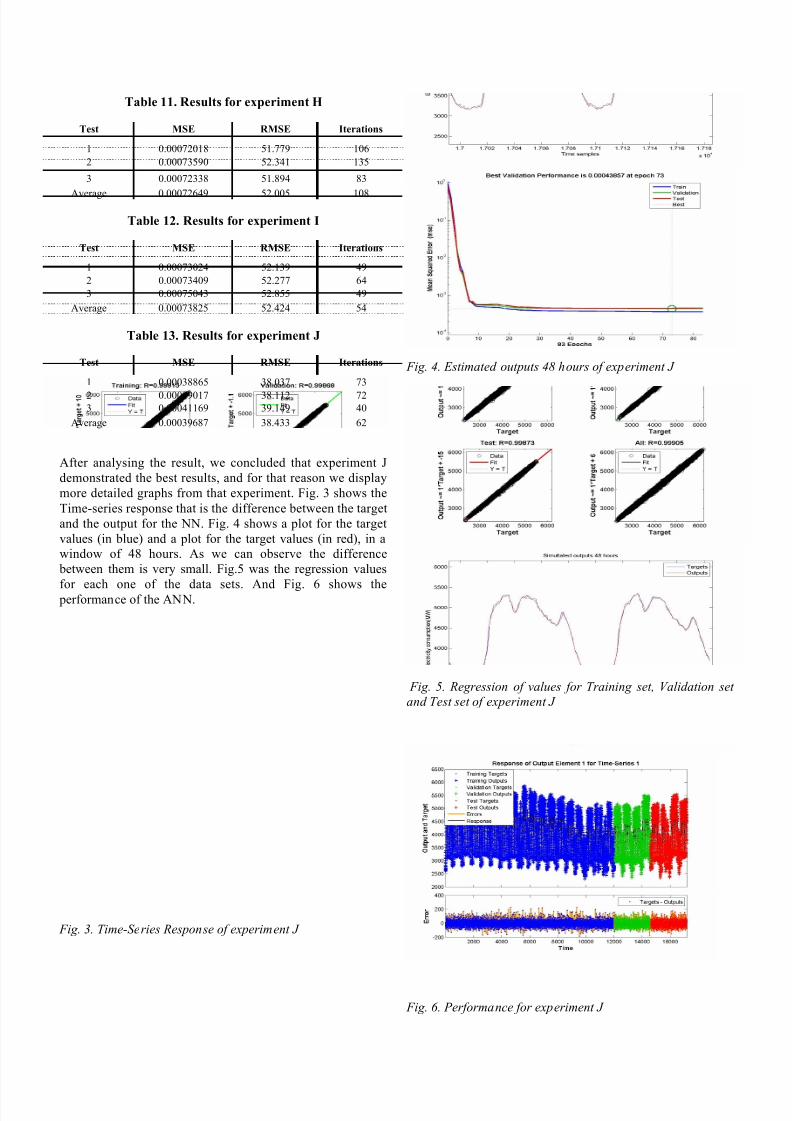
After analysing the result, we concluded that experiment J

demonstrated the best results, and for that reason we display

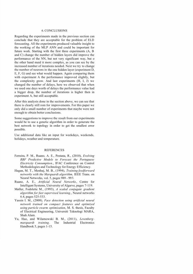
more detailed graphs from that experiment. Fig. 3 shows the

Time-series response that is the difference between the target

and the output for the NN. Fig. 4 shows a plot for the target

values (in blue) and a plot for the target values (in red), in a

window of 48 hours. As we can observe the difference

between them is very small. Fig.5 was the regression values

for each one of the data sets. And Fig. 6 shows the performance of the ANN.

Fig. 3. Time-Series Response of experiment J

Fig. 4. Estimated outputs 48 hours of experiment J

Fig. 5. Regression of values for Training set, Validation set

and Test set of experiment J

Fig. 6. Performance for experiment J



6. CONCLUSIONS

Regarding the experiments made in the previous section can

conclude that they are acceptable for the problem of ELD

forecasting. All the experiments produced valuable insight to

the working of the MLP ANN and could be important forfuture work. Starting with the first three experiments (A, B

and C) change the number of hidden layers did improve the

performance of the NN, but not very significant way, but o

the other hand maid it more complex, as you can see by the

increased number of iterations needed. Next we try to change

the number of neurons in the one hidden layer (experiment D,

E, F, G) and see what would happen. Again comparing them

with experiment A the performance improved slightly, but

the complexity grow. And last experiments (H, I, J) we

changed the number of delays, here we observed that when

we used one days worth of delays the performance value had

a bigger drop, the number of iterations is higher then in

experiment A, but still acceptable.

After this analysis done in the section above, we can see that

there is clearly still rom for improvements. For this paper we

only did a small number of experiments that maybe were not

enough to obtain better conclusions.

Some suggestions to improve the result from our experiments

would be to use a genetic algorithm in order to generate the

best network to topology in order to get the smallest error

possible.

Use additional data like an input for weekdays, weekends,

holidays, weather and temperature.

REFERENCES

Ferreira, P. M., Ruano, A. E., Pestana, R., (2010), Evolving

RBF Predictive Models to Forecast the Portuguese

Electricity Consumption., IFAC Conference on Control

Methodologies and Technology for Energy Efficiency.

Hagan, M. T., Menhaj, M. B., (1994), Training feedforward

networks with the Marquardt algorithm, IEEE Trans. on

Neural Networks, vol. 5, pages 989 - 993. Ruano, A. E., Artificial Neural Networks, Centre for

Intelligent Systems, University of Algarve, pages 7-119. Møller, Fodslette M., (1993), A scaled conjugate gradient

algorithm for fast supervised learning ., Neural networks6.4, pages 525-533.

Yassin I. M., (2008), Face detection using artificial neural

network trained on compact features and optimized

using particle swarm optimization, M. S. thesis, Faculty

of Electrical Engineering, Universiti Teknologi MARA,

Shah Alam.

Yu, Hao, and Wilamowski B. M., (2011), Levenberg-

marquardt training. The Industrial Electronics

Handbook 5, pages 1-15.

Documents

ELD ANN MLP