emt - Bhattadev University

Dr.

UpakulMahanta,DepartmentofPhysics,Bhattadev

University

ELECTROMAGNETIC THEORY

BY

DR. UPAKUL MAHANTA,

Asst.Prof., Department of Physics,Bhattadev University

BSc. 6th Sem./ MSc. 2nd Sem. Class notes

Dr. Upakul Mahanta, Department of Physics, Bhattadev University

Dr.


University

Contents

1 EM Waves & Maxwell’s Field Equations 51.1 Introduction . . . . . . . . . . . . . . . . . . . . . . . . . . . . . . . . . . . . . . . . . . . . . . . . . . . 51.2 Basics & Terminologies . . . . . . . . . . . . . . . . . . . . . . . . . . . . . . . . . . . . . . . . . . . . 51.3 Basic vector opearation . . . . . . . . . . . . . . . . . . . . . . . . . . . . . . . . . . . . . . . . . . . . 6

1.3.1 E -M Waves . . . . . . . . . . . . . . . . . . . . . . . . . . . . . . . . . . . . . . . . . . . . . . . 61.3.2 Properties of E -M Waves . . . . . . . . . . . . . . . . . . . . . . . . . . . . . . . . . . . . . . . 6

1.4 Maxwell’s Field Equations . . . . . . . . . . . . . . . . . . . . . . . . . . . . . . . . . . . . . . . . . . . 71.4.1 Maxwell’s equation, Gauss Law for electrostatics . . . . . . . . . . . . . . . . . . . . . . . . . . 71.4.2 Maxwell’s second equation . . . . . . . . . . . . . . . . . . . . . . . . . . . . . . . . . . . . . . . 71.4.3 Maxwell’s third equation, Faraday’s law of EM induction . . . . . . . . . . . . . . . . . . . . . 81.4.4 Maxwell’s fourth equation, Modification of Ampere’s law . . . . . . . . . . . . . . . . . . . . . 9

1.5 Maxwell’s four equations: . . . . . . . . . . . . . . . . . . . . . . . . . . . . . . . . . . . . . . . . . . . 101.6 Explicit solutions of Maxwell’s equations . . . . . . . . . . . . . . . . . . . . . . . . . . . . . . . . . . . 10

2 Propagation of Electro-Magnetic Waves 112.1 Medium Characteristics . . . . . . . . . . . . . . . . . . . . . . . . . . . . . . . . . . . . . . . . . . . . 112.2 Propagation of EM waves in Free Space ie σ = 0, & ρ = 0 . . . . . . . . . . . . . . . . . . . . . . . . 112.3 Impedance of free space . . . . . . . . . . . . . . . . . . . . . . . . . . . . . . . . . . . . . . . . . . . . 122.4 Propagation of EM waves in Conducting Medium ie, σ 6= 0 . . . . . . . . . . . . . . . . . . . . . . . . 13

2.4.1 Attenuation . . . . . . . . . . . . . . . . . . . . . . . . . . . . . . . . . . . . . . . . . . . . . . . 152.4.2 Skin Depth . . . . . . . . . . . . . . . . . . . . . . . . . . . . . . . . . . . . . . . . . . . . . . . 15

2.5 Propagation of EM waves in a Dielectric Medium ie σ = 0 . . . . . . . . . . . . . . . . . . . . . . . . 162.6 Poynting Theoram . . . . . . . . . . . . . . . . . . . . . . . . . . . . . . . . . . . . . . . . . . . . . . . 16

2.6.1 Derivation of Poynting Theoram . . . . . . . . . . . . . . . . . . . . . . . . . . . . . . . . . . . 172.7 Relationship between ~E and ~B magnitudes . . . . . . . . . . . . . . . . . . . . . . . . . . . . . . . . . 182.8 Time averaged value of the Poynting Vector, 1

µ0

( ~E × ~B) . . . . . . . . . . . . . . . . . . . . . . . . . . 19

2.8.1 Energy contribution from the ~E and ~B fields . . . . . . . . . . . . . . . . . . . . . . . . . . . . 19

3 Reflection, Refraction (Transmission) and Polarization of Electro-Magnetic Waves 213.1 Introduction . . . . . . . . . . . . . . . . . . . . . . . . . . . . . . . . . . . . . . . . . . . . . . . . . . . 213.2 Reflection, and Transmission of EM Waves at a boundary (interface) of two media in normal incidence 21

3.2.1 Value of the Reflection (R) and Transmission (T) coefficient in terms of Poynting vector . . . . 233.3 Reflection and Transmission of EM Waves for oblique incidence : Laws of Reflection and Refraction . 233.4 Fresnel Equations . . . . . . . . . . . . . . . . . . . . . . . . . . . . . . . . . . . . . . . . . . . . . . . . 25

3.4.1 When the ~E is perpendicular to the plane of incidence: Transverse Electric . . . . . . . . . . . 253.4.2 When the ~E is parallel to the plane of incidence: Transverse Magnetic . . . . . . . . . . . . . . 27

3.5 Brewster’s law . . . . . . . . . . . . . . . . . . . . . . . . . . . . . . . . . . . . . . . . . . . . . . . . . 293.5.1 Derivation of Brewster’s law . . . . . . . . . . . . . . . . . . . . . . . . . . . . . . . . . . . . . . 30

3.6 Polarization of EM wave . . . . . . . . . . . . . . . . . . . . . . . . . . . . . . . . . . . . . . . . . . . . 313.6.1 Linnear Polarization: . . . . . . . . . . . . . . . . . . . . . . . . . . . . . . . . . . . . . . . . . . 313.6.2 Circular Polarization: . . . . . . . . . . . . . . . . . . . . . . . . . . . . . . . . . . . . . . . . . 313.6.3 Elliptical Polarization: . . . . . . . . . . . . . . . . . . . . . . . . . . . . . . . . . . . . . . . . . 32

3

Dr. Upakul Mahanta, Department of Physics, Bhattadev University

Dr.


University

Chapter 1

EM Waves & Maxwell’s Field Equations

1.1 Introduction

Perhaps the greatest theoretical achievement of physics in the 19th century was the discovery of electromagnetic waves.The history of electromagnetic theory begins with ancient measures to understand atmospheric electricity, in particularlightning, but were unable to explain the phenomena. People then had little understanding of electricity except thesefacts. Electric forces in nature come in two kinds. First, there is the electric attraction between unlike (+) and (−)charges or repulsion between like (+) and (+) or (−) and (−) electric charges. It is possible to use this to define aunit of electric charge, as the charge which repels a similar charge at a distance of, say, 1 meter, with a force of unitstrength.Then Faraday showed that a magnetic field which varied in time like the one produced by an alternating current(AC) could drive electric currents, if (say) copper wires were placed in it in the appropriate way. That was “magneticinduction,” the phenomenon on which electric transformers are based. So, magnetic fields could produce electriccurrents, and we already know that electric currents produce magnetic fields. In the 19th century it had become clearthat electricity and magnetism were related, and their theories were unified: wherever charges are in motion electriccurrent results, and magnetism is due to electric current. The source for electric field is electric charge, whereas thatfor magnetic field is electric current (charges in motion).In 1864 Maxwell theoritically proposed that electromagnetic disturbance travels in free space with the speed of light.Although the idea was remain hidden in his set of equations but virtually never said anything about the waves nor hesaid anything about the generation of such waves. Later on• Hertz in 1888 succeeded in producing and observing electromagnetic waves of wavelength of the order of 6m in thelaboratory.• J. C. Bose in 1895 succeeded in producing and observing electromagnetic waves of much shorter wavelength 25 mm- 5 mm.• G. Marconi in the same year succeeded in transmitting electromagnetic waves over distances of many kilometers.

1.2 Basics & Terminologies

Whereas the Lorentz force law characterizes the observable effects of electric and magnetic fields on charges, Maxwellsequations characterize the origins of those fields and their relationships to each other. The simplest representation ofMaxwells equations is in differential form, which leads directly to waves. But before going to the Maxwell’s equationslet us refresh ourself with few terminologies which will have regular appearances in the equations. The four Maxwell

Field variables Names Unit~E Electric Field volts/meter; Vm−1

~H Magnetic Intensity amperes/meter; Am−1

~B Magnetic Flux Density Tesla, T~D Electric Displacment coulombs/m2; Cm−2

~J Electric current density amperes/m2; Am−2

ρ Electric charge density coulombs/m3; Cm−3

equations which will be derived in the next section invoke one scalar and five vector quantities comprising 16 variables.Some variables only characterize how matter alters field behavior. In vacuum we can eliminate three vectors (9

variables) by noting ~D = ǫ0 ~E, ~B = µ0~H and ~J = ρ~v = σ ~E. where ǫ0 = 8.8542× 10−12 [farads m−1] is the absolute

permittivity of vacuum, µ0 = 4π × 10−7 [henries m−1] is the absolute permeability of vacuum, ~v is the driftvelocity of the local net charge density ρ, and σ is the conductivity of a medium [Siemens m−1]. If we regard the

5

Dr.


University

electrical sources ρ and ~J as given, then the equations can be solved for all remaining unknowns. Specifically, we canthen find ~E and ~B, and thus compute the forces on all charges present.

1.3 Basic vector opearation

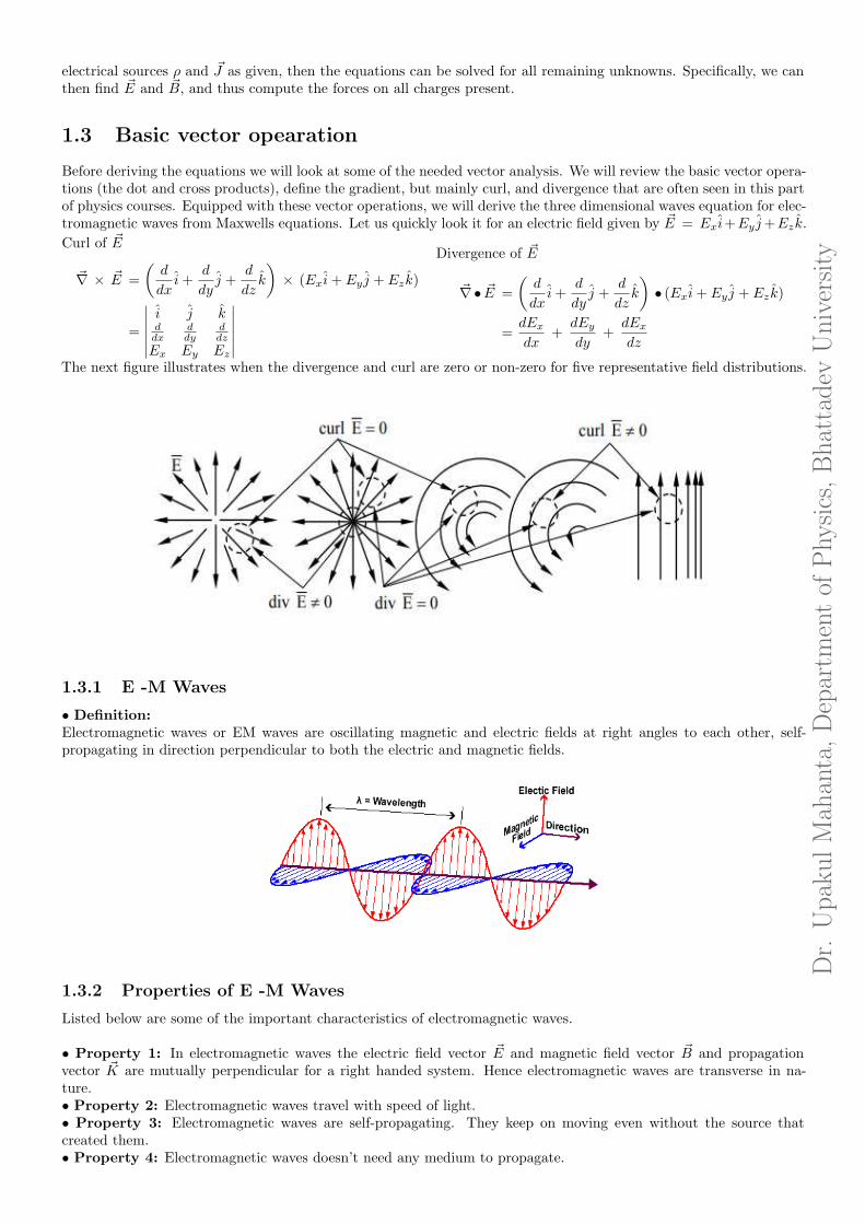
Before deriving the equations we will look at some of the needed vector analysis. We will review the basic vector opera-tions (the dot and cross products), define the gradient, but mainly curl, and divergence that are often seen in this partof physics courses. Equipped with these vector operations, we will derive the three dimensional waves equation for elec-tromagnetic waves from Maxwells equations. Let us quickly look it for an electric field given by ~E = Exi+Ey j+Ez k.

Curl of ~E

~∇ × ~E =

(

d

dxi+

d

dyj +

d

dzk

)

× (Exi+ Ey j + Ez k)

=

∣

∣

∣

∣

∣

∣

i j kddx

ddy

ddz

Ex Ey Ez

∣

∣

∣

∣

∣

∣

Divergence of ~E

~∇• ~E =

(

d

dxi+

d

dyj +

d

dzk

)

• (Exi+ Ey j + Ez k)

=dEx

dx+

dEy

dy+

dEx

dz

The next figure illustrates when the divergence and curl are zero or non-zero for five representative field distributions.

1.3.1 E -M Waves

• Definition:Electromagnetic waves or EM waves are oscillating magnetic and electric fields at right angles to each other, self-propagating in direction perpendicular to both the electric and magnetic fields.

1.3.2 Properties of E -M Waves

Listed below are some of the important characteristics of electromagnetic waves.

• Property 1: In electromagnetic waves the electric field vector ~E and magnetic field vector ~B and propagationvector ~K are mutually perpendicular for a right handed system. Hence electromagnetic waves are transverse in na-ture.• Property 2: Electromagnetic waves travel with speed of light.• Property 3: Electromagnetic waves are self-propagating. They keep on moving even without the source thatcreated them.• Property 4: Electromagnetic waves doesn’t need any medium to propagate.

Dr.


University

• Property 5: Electromagnetic waves are not deflected by electric or magnetic field.• Property 6: Electromagnetic waves can show interference or diffraction and can be polarized.• Property 7: Electromagnetic waves carry energy with them and exerts pressure on the medium they incident upon.

1.4 Maxwell’s Field Equations

From a long view of the history of mankind seen from, say, ten thousand years from now, there can be little doubt that the most significant

event of the 19th century will be judged as Maxwell’s discovery of the laws of electrodynamics.

. The Feynman Lectures on Physics (1964), Richard Feynman

Maxwell’s equations are a set of four differential equations that, together with the Lorentz force law, form the foun-dation of classical electromagnetism, classical optics, and electric circuits. These equations describe how electric andmagnetic fields propagate, interact, and how they are influenced by objects. He was an Einstein/Newton-level geniuswho took a set of known experimental laws (Faraday’s Law, Ampere’s Law) and unified them into a symmetric coherentset of Equations known as Maxwell’s Equations. Maxwell was one of the first to determine the speed of propagationof electromagnetic (EM) waves was the same as the speed of light - and hence to conclude that EM waves and visiblelight were really the same thing.The four Maxwell’s equations can be divided into two major subsets. The first two, Gauss’s law for electrostatics andone people used to say as Gauss’s law for magnetism, however it is not exactly so, describe how fields emanate fromcharges and magnets respectively. The other two, Faradays law and Ampere’s law with Maxwell’s correction, describehow induced electric and magnetic fields circulate around their respective sources.Each of Maxwell’s equations can be looked at from the “microscopic” perspective, which deals with total charge andtotal current, and the “macroscopic” set, which defines two new auxiliary fields that allow one to perform calculationswithout knowing microscopic data like charges at the atomic level.

Let us now discuss them one by one.

1.4.1 Maxwell’s equation, Gauss Law for electrostatics

The integral of the outgoing electric field ~E over an area enclosing a volume V equals the total charge Q enclosed bythe volume divided by ǫ0 in vacuum. Mathematically Gauss’ law is

{

S

~E • ~dS =Qenc

ǫ0

But this can be written as an equality between three dimensional volume integrals, by writing the total charge enclosedQ as the integral of the charge density over the volume, using the Gauss’ divergence theorem (in fact it is due to him)

{

S

~E • ~dS =1

ǫ0

y

V

ρ dV

y

V

(~∇• ~E) dV =1

ǫ0

y

V

ρ dV

~∇• ~E =ρ

ǫ0

Where ρ is the volume charge density.It represents completely covering the surface with a large number of tiny patches having areas ~dS. We represent thesesmall areas as vectors pointing outwards, because we can then take the dot product with the electric field to selectthe component of that field pointing perpendicularly outwards (it would count negatively if the field were pointinginwards) - this is the only component of the field that contributes to actual flow across the surface. (Just as a riverflowing parallel to its banks has no flow across the banks).

• Physical Significance:The net quantity of the electric flux leaving a volume is proportional to the charge inside the volume.

1.4.2 Maxwell’s second equation

The second law states that there are no “magnetic charges (or monopoles)” analogous to electric charges, and thatmagnetic fields are instead generated by magnetic dipoles. Such dipoles can be represented as loops of current, but inmany ways are similar in appearance to positive and negative “magnetic charges” that are inseparable and thus haveno formal net “magnetic charge.” This can be derived from Biot-Savart Law

Dr.


University

If B(r) is the magnetic flux at the point r and J(r) is the current density at the point r′ then Biot-Savart Law is givenby

B (r) =µ0

4π

ˆ

V

~J(r) dv × r∣

∣r − r′∣

∣

2

~∇•B (r) =µ0

4π

ˆ

V

~∇•~J(r) dv × r∣

∣r − r′∣

∣

2

To carry through the divergence of the integrand in the above equation, we will use the vector identity given by~∇• (A × B) = ~B • (∇ × B) − ~A • (∇ × B)

~∇•B (r) =µ0

4π

ˆ

V

[

~J(r) •(

∇ × r∣

∣r − r′∣

∣

2

)]

dv −ˆ

V

[

r∣

∣r − r′∣

∣

2 •(

∇ × ~J(r))

]

dv

The first part of RHS of the above equation is zero as the curl ofr

∣

∣r − r′∣

∣

2 is zero. Also the second part of RHS of

the above equation becomes zero because J(r) depends on r′ and ∇ depends only on r. Plugging this back into, theright-hand side of the expression becomes zero. Thus, we see that

~∇• ~B = 0

Another way of doing the same thing is the following{

S

~B • ~dS = 0

Now applying the Gauss’ divergence theorem to the above equation we gety

V

(~∇• ~B) dV = 0

~∇• ~B = 0

Magnetic field lines form loops such that all field lines that go into an object leave it at some point. Thus, the totalmagnetic flux through a surface surrounding a magnetic dipole is always zero.

• Physical Significance:Magnetic monopole doesnot exsist.

1.4.3 Maxwell’s third equation, Faraday’s law of EM induction

Faraday demonstrated the fact that whenever the magnetic flux associated with any closed loop changes an inducedemf developes in the circuit and that sends current through the circuit which last so long as the change of flux lasts.He also showed that the induced emf produced is directly proporsonal to magnetic flux linked with the coil. Inmathematical language Faradays law states that the closed integral of the induced electric field is minus the time rateof change of the magnetic flux through the loop. Or simply saying a time-varying magnetic field (or flux) induces anelectric field. In fact the straight forward outcome of this equation says that work is needed to take a charge arounda closed curve in an electric field.Thus the mathematical form is

E = − dΦB

dt˛

C

~E • ~dl = − ∂ΦB

∂ t˛

C

~E • ~dl = −x

S

∂ ~B

∂ t• ~dS

where E is the induced emf. It may seem that the integral on the right hand side is not very clearly defined, becauseif the path or circuit lies in a plane, the natural choice of spanning surface is flat, but how do you decide what surfaceto choose to do the integral over for a wire bent into a circuit that doesn’t lie in a plane? The answer is that it doesn’tmatter what surface you choose, as long as the wire forms its boundary. Now applying Stokes’ theoram in the aboveequation we get

{

S

(~∇ × ~E) • ~dS = −{

S

∂ ~B

∂ t• ~dS

~∇ × ~E = −∂ ~B

∂ t

Dr.


University

The divergence of the left hand side of Faraday’s law, ~∇•(~∇ × ~E), vanishes identically so if Faradays law is consistent

it must be true that ~∇•∂ B∂ t

also vanishes. Since the time and space partial derivatives commute, this is the same asddt

~∇•B, which vanishes thanks to the second law. So the absense of magnetic charges is required for Faraday’s lawto be self-consistent.

• Physical Significance:A time varying magnetic field linked with a loop produces an induced emf in the loop which in turn produces a spacevarying electric field.

1.4.4 Maxwell’s fourth equation, Modification of Ampere’s law

Amperes law states that the line integral of the magnetic field ~B around any closed path or circuit is equal to thecurrent enclosed by the path. In a simple note magnetic field could be created by electrical current. ie

˛

C

~B • ~dl = µ0 I

The I in Ampere’s law is called the conduction current, iedQ

dt. But this Ampere’s law is in its incomplete form. Why?

Because from here we can show that ~∇ × ~B = µ0~J . Now taking divergence in this equation the left hand side vanishes.

ie ~∇•~∇ × ~B = 0. But the at the same time the right hand side doesn’t go off since according to equation of continuity∂ ρ∂ t

+ ~∇• ~J = 0 which gives ~∇• ~J = −dρdt. In a steady state situation, where all time derivatives vanish, Ampre’s law is

self-consistent. However in the presence of time dependent charge densities it cannot be correct. Because here electricfield which grows continuously since there has been an accumulation of charge in the capacitor plates. Thus there isa time varying electric field present between the plates. That implies there must also a magnetic field present insidethe capacitor plate. And then if you place a compass needle between the capacitor plates the needle gets displaced iethere is some deflection. So the point here is that between the plates no conductor is there ie no conduction currentshould be there but still the needle is showing deflection and the circuit shows a current reading. Maxwell resolvedthis contradiction by creating something called a displacement current. This was an analogy with a dielectric material.If a dielectric material is placed in an electric field, the molecules are distorted, their positive charges moving slightlyto the right, say, the negative charges slightly to the left. Now consider what happens to a dielectric in an increasingelectric field. The positive charges will be displaced to the right by a continuously increasing distance, so, as long asthe electric field is increasing in strength, these charges are moving: there is actually a displacement current. Thiselectric field that produces the current and makes the circuit continuous. Maxwell added this displacement term inAmpere’s law and he showed that it is equal to the permittivity of free space times the rate of change of electric fluxwith respect to time. Let us now see how this was achieved.

C =Q

Vǫ0 A

d=

Q

V

Q = ǫ0 AV

d

dQ

dt= ǫ0 A

d~E

dt

ID = ǫ0 Ad~E

dt

where ID is the displacement current and other symbols have their usual meaning. Thus Maxwell modified theAmperes law to

˛

C

~B • ~dl = µ0 (I + ID)

Now the above equation can be rewritten as˛

C

~B • ~dl = µ0

[{

S

~J• ~dS +{

S

ǫ0d ~E

dt• ~dS

]

x

S

(~∇ × ~B) • ~dS = µ0

[x

S

~J• ~dS +x

S

ǫ0d ~E

dt• ~dS

]

~∇ × ~B = µ0

[

~J + ǫ0d ~E

dt

]

Dr.


University

Therefore, this is the way to generalize Ampere’s law from the magnetostatic situation to the case where charge den-sities are varying with time.

• Physical Significance:Magnetic field B around any closed path or circuit is equal to the conductions current plus the time derivative ofelectric displacement through any surface bounded by the path.

1.5 Maxwell’s four equations:

Equation No. Equation Remark

1 ~∇• ~E = ρǫ0

Gauss law for electrostatics

2 ~∇• ~B = 0 No name

3 ~∇ × ~E = −∂ ~B∂ t

Faraday’s law of Electro-magnetic induction

4 ~∇ × ~B = µ0

[

~J + ǫ0∂ ~E∂ t

]

Maxwell’s modification of Ampere’s law

1.6 Explicit solutions of Maxwell’s equations

As we have come to know that these celebrated Maxwell’s equations are responsible for any of electro-magneticphenomenon in fact for every electro-magnetic phenomenon. So it is much desired to have the solutions for ~E and ~B

fields. Using the principles of vector algebra we find that

~∇• ~B = 0

~B = ~∇ × ~A

Here ~A is the magnetic vector potential which is not directly associated with work the way that scalar potential is.One rationale for the vector potential is that it may be easier to calculate the vector potential than to calculate themagnetic field directly from a given source current geometry. (you don’t need to think about it very much! Just

remember it). Now putting this value of ~B in Maxwell’s 3rd equation we get

~∇ × ~E = −∂ ~B

∂ t

~∇ × ~E = − ∂

∂ t(~∇ × ~A)

~∇ ×[

~E +∂ ~A

∂ t

]

= 0

~E +∂ ~A

∂ t= −∇Φ

~E = −∇Φ − ∂ ~A

∂ t

Where Φ is the scalar potential. Thus because of a changing magnetic field the curl of the electric field becomes non-zero and we donot need to abandon ~E is not a conservative field. The last equation tells us that the scalar potential Φonly describes the conservative electric field generated by electric charges. The electric field induced by time-varyingmagnetic fields is non-conservative, and is described by the magnetic vector potential ~A.

Dr.


University

Chapter 2

Propagation of Electro-Magnetic Waves

2.1 Medium Characteristics

When we consider a medium which is “simple”, we define it by the following characteristics• Linear Medium: Here µ and ǫ are constants. In general these two are tensorial terms.

• Isotropic Medium: Here the EM wave travels at same speed in all directions. ie there is no special directionis preferred which further implies that rotational symetry is present.

• Homogeneous Medium: By this we mean that the material is uniform. ie to speak that the only one singlematerial is present in the medium which implies that the density is fixed at every point in space. Thus translationsymetry is present.

• Source-free Medium: By this we mean that charge density ie ρ = 0.

• Non-conducting Medium: Here the conductivity σ = 0. Hence current density ~J = σ ~E = 0.

2.2 Propagation of EM waves in Free Space ie σ = 0, & ρ = 0

An electromagnetic wave transports its energy through a vacuum at a speed of 3× 108 m/sec. However, Mechanicalwaves, unlike electromagnetic waves, require the presence of a material medium in order to transport their energyfrom one location to another. Following is the way by which we can show that EM wave indeed travels at the speedof light.Let us do it for the ~E. Starting with Maxwell’s third equation

~∇ × ~E = −d ~B

dt

Now taking curl on both sides we get

~∇ × (~∇ × ~E) = −~∇ × ∂ ~B

∂ t

~∇(~∇• ~E) − ∇2 ~E = − ∂

∂ t(~∇ × ~B)

Now replacing ~∇ × ~B by Maxwell’s 4th equation and ~∇• ~E by Maxwell’s 1st equation we get

~∇ ρ

ǫ0− ∇2 ~E = −µ0

d

dt

[

~J + ǫ0d ~E

dt

]

~∇ ρ

ǫ0− ∇2 ~E = −µ0

d

dt

[

~σ ~E + ǫ0

d ~E

dt

]

~∇ ρ

ǫ0− ∇2 ~E = −µ0 σ

∂ ~E

∂ t− µ0 ǫ0

d2 ~E

dt2

∇2 ~E − µ0 σ∂ ~E

∂ t− µ0 ǫ0

∂ 2 ~E

∂ t2= ~∇ ρ

ǫ0

11

Dr.


University

In free space no charge accumulation, nothing is there hence ρ = 0 and also free space conducts nothing means σ = 0.Under these two situation the above expression boils down to

∇2 ~E − µ0 ǫ0∂ 2 ~E

∂ t2= 0

∇2 ~E = µ0 ǫ0∂ 2 ~E

∂ t2

Thus we have a 2nd order differential equation where the 2nd order space derivative of function is proporsonal to the2nd order time derivative of the same function. So that’s your wave equation. And the reciprocal of the proporsonalityconstant gives the square of velocity of propagation of the function.

v2 =1

µ0 ǫ0

Now plugging in the value for µ0 = 4π × 10−7H/m and ǫ0 = 8.85 × 10−12 F/m in the above equation and simplifyingwe get

v = 3× 108 m/sec = speed of light, c

Since the value of the speed of EM-wave is similar to that the speed of light therefore a corelation can be drawn thatlight is a form of EM-wave. OR

There is another way to get to the same result. The equations are now decoupled (E has its own private equations),which certainly simplifies things, but in the process we’ve changed them from first to second order (notice all thesquares). I know that lower order implies easier to work with, but these second order equations aren’t as difficult asthey look. Raising the order has not made things more complicated, it’s made things more interesting. What we willassume is the following, a plane wave solution for the ~E. ie

~E = ~E0 ei (ωt−κz)

Therefore ∇2 ~E = −κ2 ~E and d2 ~Edt2

= −ω2 ~E. And substituting these values in the last differentail equation we get

−κ2 ~E = −µ0 ǫ0 ω2 ~E

κ2 = µ0 ǫ0 ω2

ω2

κ2=

1

µ0 ǫ0

v2 =1

µ0 ǫ0


v = 3× 108 m/sec = speed of light, c

So similar type of results can also be obtained via this method. Similarly we can also show that this is true also for~B. All you have to do is to start with Maxwell’s 4th equation and similar type of vectorial algebra.

2.3 Impedance of free space

The characteristic impedance of free space, also called the Z0 of free space, is an expression of the relationship betweenthe electric-field and magnetic-field intensities in an electromagnetic field ( EM field ) propagating through a vacuum,the analogous quantity for a plane wave travelling through a dielectric medium is called the intrinsic impedance ofthe medium. The Z0 of free space, like characteristic impedance in general, is expressed in ohms, and is theoreticallyindependent of wavelength. It is considered a physical constant. However, with the redefinition of the SI base unitswhich has been already gone into force on May 20, 1919, this value is subject to experimental measurement. Let usnow derive the of this impedance.Let us suppose that an EM wave which is propagating along z direction has ~E along x direction and ~B along y direction.From the last section we now know that electric and magnetic field vector satisfy the wave equation ie second order

space derivative is proporsonal to the second order time derivative ie ∇2 ~E = ∂ 2 ~E∂ t2

and likewise for ~B field also. And

this has a plane wave solution as ~E = ~E0 ei (ωt−κz).

Dr.


University

Now using Maxwell’s 4th equation we get

~∇ × ~B = µ0

[

~J + ǫ0d ~E

dt

]

= µ0

[

σ ~E + ǫ0d ~E

dt

]

~∇ × ~B = µ0 ǫ0d ~E

dt(for free space σ = 0)

i j k∂∂x

∂∂y

∂∂z

~Bx~By

~Bz

= µ0 ǫ0

[

∂ ~Ex

∂t+

∂ ~Ey

∂t+

∂ ~Ez

∂t

]

i j k∂∂x

∂∂y

∂∂z

0 ~By 0

= µ0 ǫ0

[

∂ ~Ex

dt

]

( ~E is along x, ~B is along y)

− ∂By

∂z= µ0 ǫ0

∂ ~Ex

∂t

i κB = µ0 ǫ0 i ω E

i κH = ǫ0 i ω E

E

H=

κ

ǫ0 ω=

1

ǫ0 c=

√

µ0

ǫ0


E

H= 376.6 ohms

Mathematically, the Z0 of free space is equal to the square root of the ratio of the permeability of free space in henrysper meter to the permittivity of free space in farads per meter. The Z0 of dry air is similar to that of free space,because dry air has little effect on permeability or permittivity. However, in environments where the air containsseawater spray, excessive humidity, heavy precipitation, or high concentrations of particulate matter, the Z0 is slightlyreduced.

2.4 Propagation of EM waves in Conducting Medium ie, σ 6= 0

The mechanism of propagation of EM waves in a medium along with the energy transport through a medium involvesthe absorption and reemission of the wave energy by the atoms of the material. When an electromagnetic waveimpinges upon the atoms of a material, the energy of that wave is absorbed. The absorption of energy causes theelectrons within the atoms to undergo vibrations. After a short period of vibrational motion, the vibrating electronscreate a new electromagnetic wave with the same frequency as the first electromagnetic wave. While these vibrationsoccur for only a very short time, they delay the motion of the wave through the medium. Once the energy of theelectromagnetic wave is reemitted by an atom, it travels through a small region of space between atoms. Once itreaches the next atom, the electromagnetic wave is absorbed, transformed into electron vibrations and then reemittedas an electromagnetic wave.The actual speed of an electromagnetic wave through a material medium is dependent upon the optical density ofthat medium. Different materials cause a different amount of delay due to the absorption and reemission process.Furthermore, different materials have their atoms more closely packed and thus the amount of distance between atomsis less. These two factors are dependent upon the nature of the material through which the electromagnetic waveis traveling. As a result, the speed of an electromagnetic wave is dependent upon the material through which it istraveling.Starting with Maxwell’s third equation

~∇ × ~E = −d ~B

dt

Now taking curl on both sides we get

~∇ × (~∇ × ~E) = −~∇ × ∂ ~B

∂ t

~∇(~∇• ~E) − ∇2 ~E = − ∂

∂ t(~∇ × ~B)

Dr.


University

Now replacing ~∇ × ~B by Maxwell’s 4th equation and ~∇• ~E by Maxwell’s 1st equation we get

~∇ρ

ǫ− ∇2 ~E = −µ

∂

∂ t

[

~J + ǫd ~E

dt

]

~∇ρ

ǫ− ∇2 ~E = −µ

∂

∂ t

[

~σ ~E + ǫ

∂ ~E

∂ t

]

~∇ρ

ǫ− ∇2 ~E = −µσ

∂ ~E

∂ t− µ ǫ0

∂ 2 ~E

∂ t2

∇2 ~E − µσ∂ ~E

∂ t− µ ǫ

∂ 2 ~E

∂ t2= ~∇ρ

ǫ

In no charge accumulation nothing is there then ρ = 0. In such cases the last expression will take the shape

∇2 ~E − µσ∂ ~E

∂ t− µ ǫ

∂ 2 ~E

∂ t2= 0

Assuming a plane wave solution for the ~E. ie

~E = ~E0 e−i (ωt−κz)

Therefore ∇2 ~E = −κ2 ~E, ∂ ~E∂ t

= −iω ~E and ∂ 2 ~E∂ t2

= −ω2 ~E. And substituting these values in the lastdifferentail equation we get

−κ2 ~E = −iσ µω ~E − µ ǫω2 ~E

−κ2 = −iσ µω − µ ǫω2

κ2 = µ ǫω2 + iσ µω

κ2 = µ ǫω2[

1 + iσ

ǫ ω

]

Thus it is clear that the square of the propagation constant is a complex quantity. Hence it is quiet legitimate toassume the propagation constant as an other complex quantity and then to equating it so that we have somethingmeaningful. So in this notion let us assume

κ = α + i β

κ2 = (α + i β)2

µ ǫω2[

1 + iσ

ǫ ω

]

= α2 − β2 + i 2αβ

Since we know the fact that for two complex numbers to be equal, then the real parts must be equal and the imaginaryparts must be equal. So one equation involving complex numbers can be written as two equations, one for the realparts, one for the imaginary parts.

α2 − β2 = µ ǫω2 and 2αβ = (µ ǫω2)σ

ǫ ω= µω σ

β =µω σ

2α

Now solving for α2 we get

α2 −[µω σ

2α

]2

= µ ǫω2

4α4 − 4α2µ ǫω2 − (µω σ)2 = 0

α2 =−(−4µ ǫω2) ±

√

(−4µ ǫω2)2 + 4× 4× µ2 ω2 σ2

2× 4

=4µ ǫω2 ±

√

16µ2 ǫ2 ω4 + 16µ2 ω2 σ2

8

=4µ ǫω2 ± 4µ ǫω2

√

1 + σ2

ǫ2 ω2

8

=µ ǫω2

2

[

1 ±√

1 +σ2

ǫ2 ω2

]

α =

√

µ ǫω2

2

[

1 ±√

1 +σ2

ǫ2 ω2

]1

2

Dr.


University

Now putting the value of α2 in α2 − β2 = µ ǫω2 and then solving for β2 we get

β2 = α2 − µ ǫω2

=µ ǫω2

2

[

1 ±√

1 +σ2

ǫ2 ω2

]

− µ ǫω2

=µ ǫω2

2

[

− 1 ±√

1 +σ2

ǫ2 ω2

]

β =

√

µ ǫω2

2

[

−1 ±√

1 +σ2

ǫ2 ω2

]1

2

But from both α and β we will drop the ”−” sign from the ± since presence of the ”−” sign doesn’t going to give usanything which is physically interpretable. This is why it is. Typical values conductivity of a metal ie the value of σis ≈ 107 mho/m and ǫ remains almost around 10−12 Farad/m. The value of frequency is generally is in the order of

Megahertz. So σ2

ǫ2 ω2 >> 1 which will then lead to a complex value for both α and β since analysis will yield√-ve nos..

Thus we have α and β given by

α =

√

µ ǫω2

2

[

1 +

√

1 +σ2

ǫ2 ω2

]1

2

and β =

√

µ ǫω2

2

[

−1 +

√

1 +σ2

ǫ2 ω2

]1

2

Thus the wave solution will be obtained by replacing the value of κ by α and β in the plane wave solution.

~E = ~E0 e−i (ωt−κz) = ~E0 e

−i [ωt− (α+i β) z]

= ~E0 e−i ωt+ i α z− i β z

= ~E0 e− β z e−i (ωt−α z)

Hence the final E field equation (a similar type of B field also) in any medium is given by

~E = ~E0 exp

−√

µ ǫω2

2

[

−1 +

√

1 +σ2

ǫ2 ω2

]1

2

z

exp

−i (ωt −√

µ ǫω2

2

[

1 +

√

1 +σ2

ǫ2 ω2

]1

2

z)

2.4.1 Attenuation

The presence of e− β z term in the equation tells that an EM wave experiences attenuation ie a rate of amplitude loss ispresent as it propagates through the medium. Attenuation defines the rate of amplitude loss an EM wave experiencesat it propagates which is defined by the parameter β. Thus

β =

√

µ ǫω2

2

[

−1 +

√

1 +σ2

ǫ2 ω2

]1

2

> 0

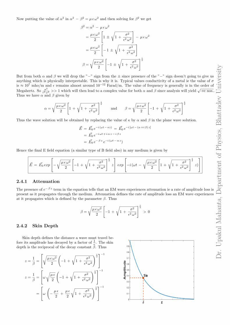
2.4.2 Skin Depth

Skin depth defines the distance a wave must travel be-fore its amplitude has decayed by a factor of 1

e. The skin

depth is the reciprocal of the decay constant β. Thus

z =1

β=

√

µ ǫω2

2

(

−1 +

√

1 +σ2

ǫ2 ω2

)1

2

−1

z =1

β=

ω

√

µ ǫ

2

(

−1 +

√

1 +σ2

ǫ2 ω2

)1

2

−1

=

ω

(

− µ ǫ

2+

µ ǫ

2

√

1 +σ2

ǫ2 ω2

)1

2

−1

Dr.


University

But in the quasi-static regime, ie for a good conductor σǫ ω

> 1. Thus the above expression will take the followingform

z =1

β=

[

ω(

− µ ǫ

2+

σ

ǫ ω

µ ǫ

2

)1

2

]−1

=

[

ω(

− µ ǫ

2+

µσ

2ω

)1

2

]−1

=

[

(

− µ ǫω2

2+

µσ ω

2

)

1

2

]−1

≈√

2

µσ ω

Thus from the last equations, we see that the skin depth decreases as the conductivity σ, magnetic permeability µ

and frequency ω increases. In most cases however, the magnetic properties are negligible as µ ≈ µ0.

2.5 Propagation of EM waves in a Dielectric Medium ie σ = 0

We now consider electromagnetic waves propagating in a dielectric medium. We suppose that the medium is notmagnetized, and we further assume that the waves are propagating in the absence of free charges and currents ie noconduction of charge. Under these assumptions you just have to do all the calculation just we did in case of conductingmedium until you find the α and β which are

α =

√

µ ǫω2

2

[

1 +

√

1 +σ2

ǫ2 ω2

]1

2

and β =

√

µ ǫω2

2

[

−1 +

√

1 +σ2

ǫ2 ω2

]1

2

since my conductivity is zero, σ = 0 the value of α and β will be after putting the value of σ we get

α =

√

µ ǫω2

2

[

1 +

√

1 +σ2

ǫ2 ω2

]1

2

=

√

µ ǫω2

2(1 + 1)

1

2

=√µ ǫω

β =

√

µ ǫω2

2

[

−1 +

√

1 +σ2

ǫ2 ω2

]1

2

=

√

µ ǫω2

2(− 1 + 1)

1

2

= 0Thus it can be realised that

κ = α + i β = α

=√µ ǫω

ω

κ=

1√µ ǫ

=1√

µr µ0 ǫr ǫ0

Vel. of the wave, v =c√µr ǫr

Thus it is seen that the there will be propagation of the EM wave even in the medium, but the velocity will be lessthan the speed of light since µr & ǫr > 1. How much slower? Here is your answer. Let us assume that the medium isnon-magnetic material, hence µr = 1 and this will result the following

v =c√ǫr

c

v=

√ǫr

Refractive index of the mediumn =√ǫr

Hence, we conclude that electromagnetic waves propagate through a dielectric medium slower than through a vacuumby a factor n. This conclusion (which was reached long before Maxwell’s equations were invented) is the basis of allgeometric optics involving refraction.

2.6 Poynting Theorem

Perhaps the heart of electro-magnetic theory. Let us consider a case where an electromagnetic field confined to a givenvolume. Now let me ask you a question. How does the energy contained in the field, change? And the answer isactually there are two processes by which it can happen. The first is by the mechanical work done by the electromag-netic field on the currents, which would appear as Joule heat and the second process is by radiative flow of energyacross the surface of the volume. Thus in electrodynamics, Poynting’s theorem is a statement of conservationof energy for the electromagnetic field. It is analogous to the work-energy theorem in classical mechanics, andmathematically similar to the continuity equation, because it relates the energy stored in the electromagnetic field tothe work done on a charge distribution (i.e. an electrically charged object), through energy flux.

Dr.


University

•The Statement: Version IThe rate of energy transfer (per unit volume) from a region of space equals to the rate of work done which will bestored on a charge distribution plus the energy flux leaving out of that region.•The Statement: Version IIThe decrease in the electromagnetic energy per unit time in a certain volume is equal to the sum of work done by thefield forces and the net outward flux per unit time.•The Statement: Version IIIThe time rate of change of electromagnetic energy within a volume V plus the net energy flowing out of that volumethrough a surface S per unit time is equal to the negative of the total work done on the charges within the volume V.You can write whichever you want in your exam. All are equivalent.

2.6.1 Derivation of Poynting Theoram

Consider first a single particle of charge Q traveling with a velocity vector ~v. Let ~E and ~B be electric and magneticfields external to the particle; i.e., ~E and ~B do not include the electric and magnetic fields generated by the movingcharged particle. The force on the particle is given by the Lorentz formula

F = Q[

~E + (~v × ~B)]

Now if this force displaces a the charge by an elementary amount d~l then the workdone on the particle is given by

dW = F • d~l = Q[

~E + (~v × ~B)]

• d~l

= Q[

~E + (~v × ~B)]

•~vdt

= Q[

~E •~vdt]

+ Q[

(~v × ~B)]

•~vdt

The second part of right hand side ie the work done by the magnetic field on the particle is zero because the force dueto the magnetic field is perpendicular to the velocity vector ~v. Thus we are only left with

dW = Q[

~E •~vdt]

dW

dt= Q ~E •~v

The last equation can be further solved with a little bit of dimensional analysis. See charge is coulomb, C and velocity

is distance over time ie LT. Hence coulomb per time is current I and current per area is current density ~J and in the

numerator the left alone L is getting multiplied by area ie L2 to give rise to L3 ie volume V. Thus

dW

dt= ~E • ~J V =

ˆ

V

~E • ~J dV

Now from of the Ampere-Maxwell’s Law

~∇ × ~B = µ0

[

~J + ǫ0d ~E

dt

]

1

µ0

(

~∇ × ~B)

= ~J + ǫ0d ~E

dt

~J =1

µ0

(

~∇ × ~B)

− ǫ0d ~E

dtˆ

V

~E • ~J dV =

ˆ

V

~E •[

1

µ0

(

~∇ × ~B)

− ǫ0d ~E

dt

]

dV

=1

µ0

ˆ

V

[

~E •(

~∇ × ~B)]

dV − ǫ0

ˆ

V

(

~E • d ~E

dt

)

dV

=1

µ0

ˆ

V

[

~B •(

~∇ × ~E)

− ~∇•(

~E × ~B)]

dV − ǫ0

ˆ

V

(

~E • d ~E

dt

)

dV (vector idenity, Sem I)

=1

µ0

ˆ

V

[

~B •(

−d ~B

dt

)

− ~∇•(

~E × ~B)

]

dV − ǫ0

ˆ

V

(

~E • d ~E

dt

)

dV (Maxwell’s 3rd equn)

Dr.


University

=1

2µ0

ˆ

V

[

−d(

B2)

dt− ~∇•

(

~E × ~B)

]

dV − ǫ0

2

ˆ

V

d(

E2)

dtdV

= − d

dt

ˆ

V

[

1

2

(

ǫ0 E2 +

1

µ0B2

)]

dV − 1

µ0

ˆ

V

[

~∇•(

~E × ~B)]

dV

ˆ

V

~E • ~J dV = − d

dt

ˆ

V

[

1

2

(

ǫ0 E2 +

1

µ0B2

)]

dV −ˆ

S

1

µ0

(

~E × ~B)

• dS

which is the work-energy theoram in elctrodynamics. Thus it says that work done by the electric and magnetic fieldson the charges within a volume must match the rate of decrease of the energy of the fields within that volume and thenet flow of energy into the volume. The big question is what does the net flow of energy into the volume correspondto physically? One possibility is that it might correspond to electromagnetic radiation. The above equation can alsobe stated as the negative of the work done on the charges within a volume must be equal to the increase in the energyof the electric and magnetic fields within the volume plus the net flow of energy out of the volume.Usually any difference between the change in energy and the work done is the energy of radiation. This is what isuniversally presumed in the case of the Poynting theorem, but the empirical evidence is that this cannot be so. If thePoynting vector corresponded to radiation then if a permanent magnet was placed in the vicinity of a body chargedwith static electricity the combination should glow and is that is not the case.

• Physical Significances of each term:

´

V~E • ~J dV : The term ~E • ~J is known as Joule heating; it expresses the rate of energy transfer to the charge

carriers from the fields. In other words it’s the total ohmic power dissipated within the volume. This is the (spatially)local version of an equation with which you are already familiar, P = V I . Notice that this term only contains theelectric field because the magnetic field can do no work on the charges.

ddt

´

V

[

12

(

ǫ0 E2 + 1

µ0

B2)]

dV : The rate at which electromagnetic energy is stored within the volume.

´

S1µ0

(

~E × ~B)

• dS : This term is called Poynting vector (it ’Poynts’ in the direction of energy transport).

The direction of Poynting vector is along the direction of propagation and the magnitude is the rate at which theelectromagnetic energy crosses a unit surface area perpendicular to the direction of the vector, ie it is the net flow ofenergy out of the volume V. But here there is an issue. The issue is what does the net flow of energy out of the volumecorrespond to physically. You might expect that since the dimensions of the Poynting vector term are energy per unitarea per unit time it is the electromagnetic radiation generated in the volume. But there is a major problem with thePoynting vector; it is independent of the charges involved. It is the same whether there is one charge or one hundredmillion charges, or for that matter, zero charges and at whatever velocities. It can change with time but only as aresult of the changes in the electric and magnetic fields. So the Poynting vector term apparently does not correspondto radiation. It is a puzzle as to what it does correspond to but there is no possibility that it corresponds to radiation.

2.7 Relationship between ~E and ~B magnitudes

In an electromagnetic wave, moving along one direction, ie say along z, the magnitudes of electric field and magneticfields can be expressed as function of plane wave ie

~E = ~E0 e−i (ω t−κ z) and ~B = ~B0 e

−i (ω t−κ z)

Now using Maxwell’s 3rd relationship ~∇ × ~E = −d ~Bdt

we get

~∇ × ~E =d

dz

[

~E0 e−i (ω t−κ z)

]

= i κ ~E

d ~B

dt=

d

dt

[

~B0 e−i (ω t−κ z)

]

= (−i ω ~B)Hence we get

i κ ~E = − (−i ω ~B)

~E0 e−i (ω t−κ z)

~B0 e−i (ω t−κ z)=

ω

κ

| ~E0|| ~B0|

= v velocity of the wave

If the wave is travelling in free space then the velocity will be c ie the speed of light.

Dr.


University

2.8 Time averaged value of the Poynting Vector, 1µ0( ~E × ~B)

Unfortunately we cannot blindly apply to power and energy our standard conversion protocol between frequency-domain and time-domain representations because we no longer have only a single frequency present. Time-harmonicpower and energy involve the products of sinusoids and therefore exhibit sum and difference frequencies. (Recall su-perposition of two waves, where you get bandwidth of frequencies as ± terms). That’s why we cannot simply represent

the Poynting vector ~S for a field at frequency f by Re(~S ei ω t) because power has components at both f = 0 and 2f,since ω = 2πf . Thus what we will do is we can use the convenience of the time-harmonic notation by restricting it tofields, voltages, and currents while representing their products, i.e. powers and energies.Now assuming the electric and magnetic fields is given by

~E = ~E0 ei ω t

= (ERe + i EIm) (cos ω t + i sinω t)

= ERe cos ω t − EIm sinω t

~B = ~B0 ei ω t

= (BRe + i BIm) (cos ω t + i sinω t)

= BRe cos ω t − BIm sinω t

Now the Poynting Vector ~S is given by

~S =1

µ0( ~E × ~B) =

1

µ0[(ERe cos ω t − EIm sinω t) × (BRe cos ω t − BIm sinω t)]

=1

µ0

[

(ERe × BRe) cos2 ω t − (ERe × BIm) cos ω t sinω t − (EIm × BRe) cos ω t sinω t + (EIm × BIm) sin2 ω t

]

Now taking the average of the above equation we get

µ0 < ~S > =< (ERe × BRe) >< cos2 ω t > − < (ERe × BIm) >< cosω t >< sinω t >

− < (EIm × BRe) >< cosω t >< sinω t > + < (EIm × BIm) >< sin2 ω t >

As you know that sine and cosine of angles have value lying between −1to 1 so the average value of them will be 0as like 0 lies exactly between [-1,1]. But then taking square of those shifts all the -ve values to the +ve ones so sinesquared and cosine squared values will lie then between [0,1]. So, the average value of them will be 1

2 . Hence we willget

< ~S > =1

µ0

[

1

2< (ERe × BRe) > − 0− 0 +

1

2< (EIm × BIm) >

]

=1

2µ0[< (ERe × BRe) > + < (EIm × BIm) >]

But to compute the Poynting vector the simplest way to use a real form for the both fields ~E and ~B rather than acomplex exponential representation.

2.8.1 Energy contribution from the ~E and ~B fields

Electromagnetic waves bring energy into a system by virtue of their electric and magnetic fields. These fields can exertforces and move charges in the system and, thus, do work on them. Clearly, the larger the strength of the electric andmagnetic fields, the more work they can do and the greater the energy the electromagnetic wave carries. The waveenergy is determined by the wave amplitude. But by how much amount does each field contribute to the wave energy?Let us look at that.We have Poynting vector which speaks about the flux of energy through any surface in a direction perpendicular toboth ~E and ~B fields as

ˆ

S

~S • d~S =1

µ0

ˆ

V

[

~∇•(

~E × ~B)]

dV

=1

µ0

ˆ

V

[

~B •(~∇ × ~E) − ~E •(~∇ × ~B)]

dV

=1

µ0

ˆ

V

[

~B •(

− d ~B

dt

)

− ~E •(

µ0 ǫ0d ~E

dt

)]

dV

This has been found by using Maxwell’s 3rd and 4th relationships along with putting σ = 0 (for free space). Onfurther simplifying we get

ˆ

S

~S • d~S = − d

dt

ˆ

V

[

ǫ0 E2

2+

B2

2µ0

]

dV

Thus the energy in any part of the electromagnetic wave is the sum of the energies of the electric and magnetic fields.Or equivalently saying the energy per unit volume, or energy density u, is the sum of the energy density from the

Dr.


University

electric field and the energy density from the magnetic field. Now the ratio of energy contribution from these twofields are

UE

UM

=ǫ0 E2

2B2

2µ0

=µ0 ǫ0 E

2

B2= µ0 ǫ0 c

2 = 1

UE = UM

This shows that the magnetic energy density UM and electric energy density UE are equal, despite the fact thatchanging electric fields generally produce only small magnetic fields.

Dr.


University

Chapter 3

Reflection, Refraction (Transmission) andPolarization of Electro-Magnetic Waves

3.1 Introduction

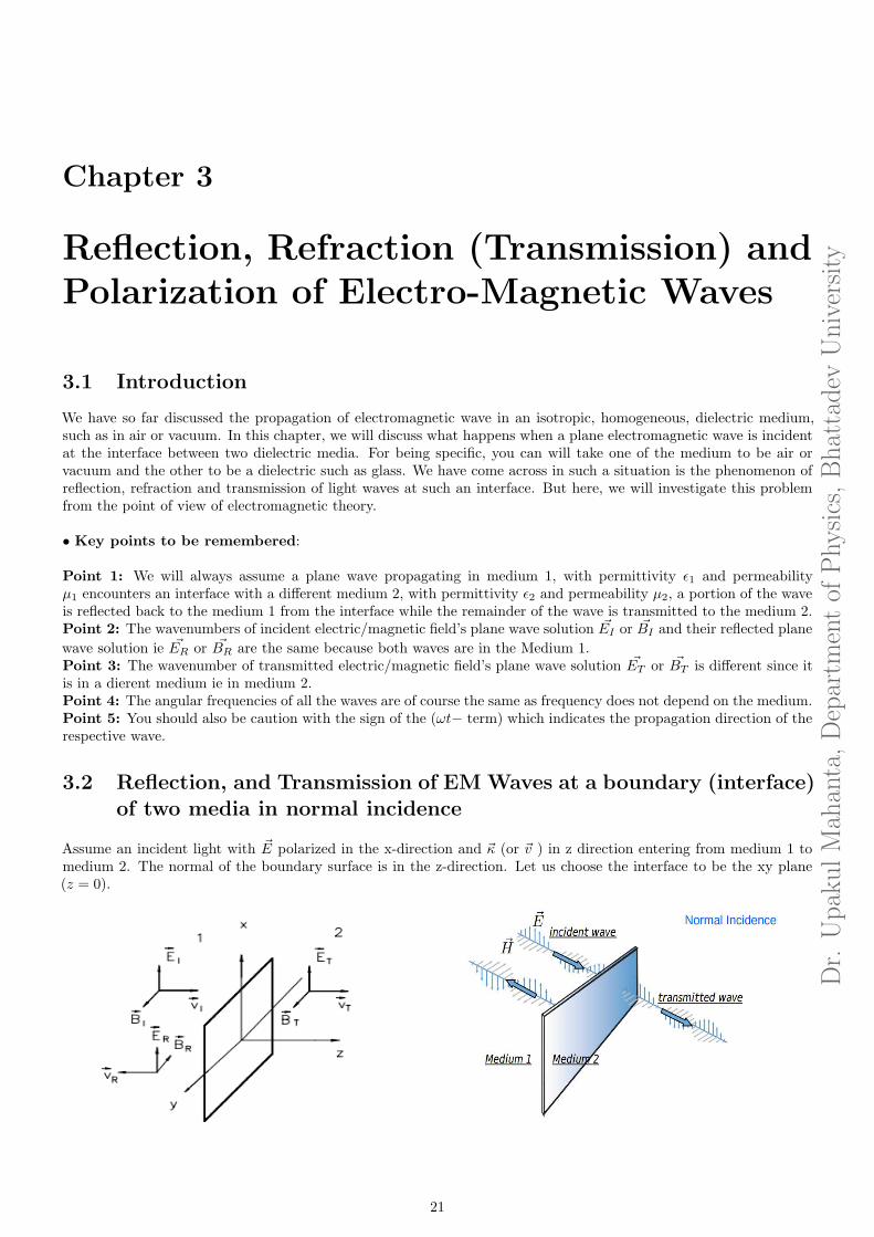
We have so far discussed the propagation of electromagnetic wave in an isotropic, homogeneous, dielectric medium,such as in air or vacuum. In this chapter, we will discuss what happens when a plane electromagnetic wave is incidentat the interface between two dielectric media. For being specific, you can will take one of the medium to be air orvacuum and the other to be a dielectric such as glass. We have come across in such a situation is the phenomenon ofreflection, refraction and transmission of light waves at such an interface. But here, we will investigate this problemfrom the point of view of electromagnetic theory.

• Key points to be remembered:

Point 1: We will always assume a plane wave propagating in medium 1, with permittivity ǫ1 and permeabilityµ1 encounters an interface with a different medium 2, with permittivity ǫ2 and permeability µ2, a portion of the waveis reflected back to the medium 1 from the interface while the remainder of the wave is transmitted to the medium 2.Point 2: The wavenumbers of incident electric/magnetic field’s plane wave solution ~EI or ~BI and their reflected plane

wave solution ie ~ER or ~BR are the same because both waves are in the Medium 1.Point 3: The wavenumber of transmitted electric/magnetic field’s plane wave solution ~ET or ~BT is different since itis in a dierent medium ie in medium 2.Point 4: The angular frequencies of all the waves are of course the same as frequency does not depend on the medium.Point 5: You should also be caution with the sign of the (ωt− term) which indicates the propagation direction of therespective wave.

3.2 Reflection, and Transmission of EM Waves at a boundary (interface)of two media in normal incidence

Assume an incident light with ~E polarized in the x-direction and ~κ (or ~v ) in z direction entering from medium 1 tomedium 2. The normal of the boundary surface is in the z-direction. Let us choose the interface to be the xy plane(z = 0).

21

Dr.


University

For the incident wave

The E field ~EI = ~E01 e−i(ω t−κ1z)x

The B field ~BI = ~B01 e−i(ω t−κ1z)y

=~E01

v1e−i(ω t−κ1 z)y

For the reflected wave

~ER = ~E01 e−i(ω t+κ1z)x

~BR = ~B01 e−i(ω t+κ1z)y

=− ~E01

v1e−i(ω t+κ1z)y

For the transmitted wave

~ET = ~E02 e−i(ω t−κ2z)x

~BT = ~B02 e−i(ω t−κ2z)y

=~E02

v2e−i(ω t−κ1z)y

Our job now is to use boundary conditions to find the complex amplitudes of the reflected and transmitted wavesin terms of that of incident wave. So, using the boundary condition that the tangential component of electric andmagnetic field is continous ie ~E|| 1= ~E|| 2 and ~B|| 1= ~B|| 2 at the interface of the two media ie at z= 0.

For the electric field at z= 0, ie on the boundary the time varying terms, e−iωt, are the same for all fields. this willimmediately give us

E0I + E0R = E0T (the orientation of the E field stays the same) .....(I)

Now for the magnetic field at z= 0, ie on the boundary

1

µ1B0I − 1

µ1B0R =

1

µ2B0T (the orientation of the B field reverses)

1

µ1 v1E0I − 1

µ1 v1E0R =

1

µ2 v2E0T

E0I − E0R =µ1 v1

µ2 v2E0T = γ E0T

[

γ =µ1 v1

µ2 v2

]

.....(II)

Now adding (I) & (II) we get

2E0I = (1 + γ)E0T .....(C)

And substracting (II) from (I) we get

2E0R = (1 − γ)E0T .....(D)Now dividing (D) by (C) we get

2E0R

2E0I=

1 − γ

1 + γ

E0R

E0I=

[

1 − µ1 v1

µ2 v2

]

[

1 + µ1 v1

µ2 v2

] =µ2 v2 − µ1 v1

µ2 v2 + µ1 v1=

√

µ2

ǫ2−√

µ1

ǫ1√

µ2

ǫ2+√

µ1

ǫ1

For free space µ1 = µ2 = µ0 (something similar to assume as non-magnetic media, µr1 = µr2 = 1) then solving outthe above equation will lead to

E0R

E0I=

√ǫ1 − √

ǫ2√ǫ1 +

√ǫ2

=n1 − n2

n1 + n2(where n s are the refractive indices)

The coefficient of reflection, R, is defined as the ratio of the intensities (nothing but the amplitude squared) of thereflected and incident waves

R =

(

E0R

E0I

)2

=

(

n1 − n2

n1 + n2

)2

Now replacing E0R from (D) and putting it in (I) we get

E0I +

(

1 − γ

2

)

E0T = E0T

E0I =1 + γ

2E0T

E0T

E0I=

2

1 + γ=

2

1 + µ1 v1

µ2 v2

=2µ2 v2

µ2 v2 + µ1 v1=

2√

µ2

ǫ2√

µ2

ǫ2+√

µ1

ǫ1

=2n2

n1 + n2(n = refractive indices)

The coefficient of transmission, T , is defined as the ratio of the intensities (nothing but the amplitude squared) ofthe transmitted and incident waves

T =

(

E0T

E0I

)2

=

(

2n2

n1 + n2

)2

Dr.


University

3.2.1 Value of the Reflection (R) and Transmission (T) coefficient in terms of Poyntingvector

Let us assume SI , SR and ST be the Ponynting vector associated with incident, reflected and transmitted wave respec-tively. Now


SI =1

µ1

(

~E0I × ~B0I

)

=E2

0I

µ1 v1


SR =1

µ1

(

~E0R × ~B0R

)

=E2

0R

µ1 v1


ST =1

µ2

(

~E0T × ~B0T

)

=E2

0T

µ2 v2

Now the coefficients are calculated as follows

The reflection coefficient

R =SR

SI

=

E2

0R

µ1 v1

E2

0I

µ1 v1

R =E2

0R

E20I

=

(

n1 − n2

n1 + n2

)2

The transmission coefficient

T =ST

SI

=

E2

0T

µ2 v2

E2

0I

µ1 v1

T =µ1 v1

µ2 v2

E20T

E20I

=n2

n1

(

2n1

n1 + n2

)2

=4n1 n2

(n1 + n2)2

Key Points to be taken away:• ~ET and ~EI are always in phase.• If n1 > n2 (glass to air), ~ER and ~EI are in phase.

• If n1 < n2 (air to glass), ~ER and ~EI are out of phase by 180o.• It is easy to show that R + T = 1, satisfying the energy conservation law. This is true even if we do not assumeµ1 ∼ µ2 ∼ µ0.

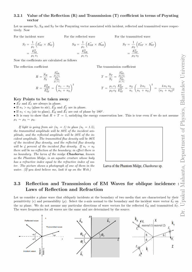
If light is going from air (n1 = 1) to glass (n1 = 1.5),the transmitted amplitude will be 80% of the incident am-plitude, and the reflected amplitude will be 20% of the in-cident amplitude. The transmitted flux density will be 96%of the incident flux density, and the reflected flux densitywill be 4 percent of the incident flux density. If n1 = n2there will be no reflection at the boundary; in effect there isno boundary. The larva of the midge Chaoborus, knownas the Phantom Midge, is an aquatic creature whose bodyhas a refractive index equal to the refractive index of wa-ter. The picture shows a photograph of one of them in thewater. (If you dont believe me, look it up on the Web.)

3.3 Reflection and Transmission of EM Waves for oblique incidence :Laws of Reflection and Refraction

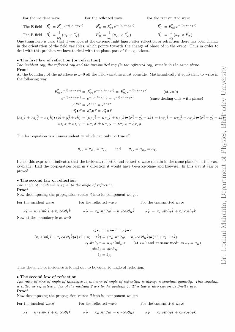
Let us consider a plane wave that obliquely incidents at the boundary of two media that are characterized by theirpermittivity (ǫ) and permeability (µ). Select the z-axis normal to the boundary and the incident wave vector ~kI on

the xz plane. We do not assume any particular directions of wave vectors for the reflected ~kR and transmitted ~kT .The wave frequencies for all waves are the same and are determined by the source.

Dr.


University


The E field ~EI = ~E01 e−i(ω t−κIr)

The B field ~BI =1

ω1(κI × ~EI)


~ER = ~E01 e−i(ω t−κRr)

~BR =1

ω1(κR × ~ER)


~ET = ~E0R e−i(ω t−κT r)

~BT =1

ω2(κT × ~ET )

One thing here is clear that if you look at the extreme right figure after reflection or refraction there has been changein the orientation of the field variables, which points towards the change of phase of in the event. Thus in order todeal with this problem we have to deal with the phase part of the equations.

• The first law of reflection (or refraction):The incident ray, the reflected ray and the transmitted ray (ie the refracted ray) remain in the same plane.ProofAt the boundary of the interface ie z=0 all the field variables must coincide. Mathematically it equivalent to write inthe following way

~E01 e−i(ω t−κIr) = ~E01 e

−i(ω t−κRr) = ~E02 e−i(ω t−κT r) (at z=0)

e−i(ω t−κIr) = e−i(ω t−κRr) = e−i(ω t−κT r) (since dealing only with phase)

ei κIr = ei κRr = ei κT r

~κI•~r = ~κR•~r = ~κT •~r(κIx i + κIy j + κIz k)• (xi+ yj + zk) = (κRx

i + κRyj + κRz

k)• (xi+ yj + zk) = (κTxi + κTy

j + κTzk)• (xi+ yj + zk)

κIx x + κIy y = κRxx + κRy

y = κTxx + κTy

y

The last equation is a linnear indentity which can only be true iff

κIx = κRx= κTx

and κIy = κRy= κTy

Hence this expression indicates that the incident, reflected and refracted wave remain in the same plane ie in this casexy-plane. Had the propagation been in y direction it would have been xz-plane and likewise. In this way it can beproved.

• The second law of reflection:The angle of incidence is equal to the angle of reflectionProofNow decomposing the propagation vector ~κ into its component we get


~κI = κI sinθI i + κI cosθI k


~κR = κR sinθR i − κR cosθRk


~κT = κT sinθT i + κT cosθT k

Now at the boundary ie at z=0

~κI•~r = ~κR•~r = ~κT •~r(κI sinθI i + κI cosθI k)• (xi+ yj + zk) = (κR sinθR i − κR cosθRk)• (xi+ yj + zk)

κI sinθI x = κR sinθR x (at z=0 and at same medium κI = κR)

sinθI = sinθR

θI = θR

Thus the angle of incidence is found out to be equal to angle of reflection.

• The second law of refraction:The ratio of sine of angle of incidence to the sine of angle of refraction is always a constant quantity. This constantis called as refractive index of the medium 2 w.r.to the medium 1. This law is also known as Snell’s law.ProofNow decomposing the propagation vector ~κ into its component we get


~κI = κI sinθI i + κI cosθI k


~κR = κR sinθR i − κR cosθRk


~κT = κT sinθT i + κT cosθT k

Dr.


University

Now at the boundary ie at z=0

~κI•~r = ~κR•~r = ~κT •~r(κI sinθI i + κI cosθI k)• (xi+ yj + zk) = (κT sinθT i + κT cosθT k)• (xi+ yj + zk)

κI sinθI x = κT sinθT x (at z=0)

sinθI

sinθT=

κT

κI

=ω√µ2 ǫ2

ω√µ1 ǫ1

=n2

n1(For non magnetic material µ = 1)

Thus the Snell’s law can be proved.

3.4 Fresnel Equations

The Fresnel equations relate the amplitudes, phases, and polarizations of the transmitted and reflected waves of elec-tric fields to the corresponding parameters of the incident waves of electric field (the waves’ magnetic fields can alsobe related using similar coefficients) which emerges when light enters an interface between two media with differentindices of refraction. When light strikes the interface between a medium with refractive index n1 and a second mediumwith refractive index n2, both reflection and refraction of the light may occur. In fact, the intensity of light reflectedfrom the surface of a dielectric, as a function of the angle of incidence was first obtained by Fresnel in 1823, as apart of his comprehensive wave theory of light. However, the Fresnel equations are fully consistent with the rigoroustreatment of light in the framework of Maxwell equations. But while deriving the equations few assumptions weremade. These are as follows

Assumptions:• The interface between the media is flat, homogeneous and isotropic.• The incident light is assumed to be a plane wave, since any incident light field can be decomposed into plane wavesand be made polarized.• Both the media are non-magnetic so that the permeability of both media are the same.• The two media differ by their dielectric constant, the incident medium may also be taken as air.• We further assume that there are no free charges or currents on the surface of interface between the two media.Electromagnetic waves follow the superposition principle. In order to simplify the math associate with our problemand derive the Fresnel equation, we split the incoming EM wave into two modesMode 1:the first case where the electric fields are perpendicular to the plane of incidence. This is case is also called asTransverse Electric and is represented by s - polarization, s standing for a German word ”senkrecht” meaningperpendicular.Mode 2:This case is known as p - polarization, p standing for ”parallel”, where the electric field is parallel to the incidentplane. A case known as Transverse Magnetic (since parallel E-field will guarantee perpendicular B-field to theplane of incidence).Let us now derive the Reflection (R) and Transmission (T) coefficient for both the two cases.

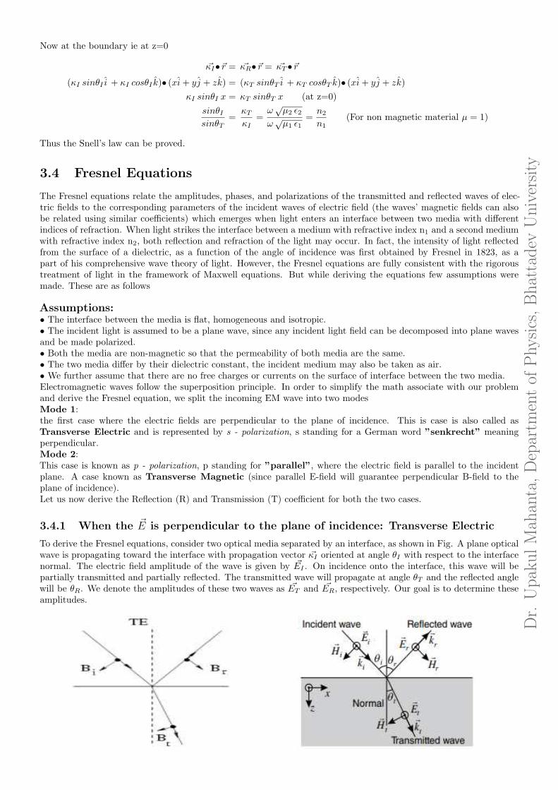
3.4.1 When the ~E is perpendicular to the plane of incidence: Transverse Electric

To derive the Fresnel equations, consider two optical media separated by an interface, as shown in Fig. A plane opticalwave is propagating toward the interface with propagation vector ~κI oriented at angle θI with respect to the interfacenormal. The electric field amplitude of the wave is given by ~EI . On incidence onto the interface, this wave will bepartially transmitted and partially reflected. The transmitted wave will propagate at angle θT and the reflected anglewill be θR. We denote the amplitudes of these two waves as ~ET and ~ER, respectively. Our goal is to determine theseamplitudes.

Dr.


University

To accomplish this, we apply the boundary conditions for the electric and magnetic fields at an interface betweentwo media with different electromagnetic properties.

1: The parallel component of ~E is continuous across the boundary between the two media.

2: The perpendicular component of ~B (but parallel component of~Bµ) is continuous across the boundary between the

two media.• The value of reflection coefficient, R

The boundary condition 1 will give

EI + ER = ET ..............(eqn. 1)

While for the magnetic field the second one will give

1

µ1BI cosθI − 1

µ1BR cosθR =

1

µ2BT cosθT

κI × EI

µ1 ω1cosθI − κR × ER

µ1 ω1cosθR =

κT × ET

µ2 ω2cosθT

√µ1 ǫ1 EI

µ1cosθI −

√µ1 ǫ1 ER

µ1cosθR =

√µ2 ǫ2 ET

µ2cosθT

√

ǫ1

µ1EI cosθI −

√

ǫ1

µ1ER cosθI =

√

ǫ2

µ2ET cosθT (since θI = θR)

√

ǫ1

µ1(EI − ER) cosθI =

√

ǫ2

µ2ET cosθT

√

ǫ1


√

ǫ2

µ2(EI + ER) cosθT (by virtue of eqn. 1)

(EI − ER)

(EI + ER)=

√

ǫ2µ2

cosθT√

ǫ1µ1

cosθI

(EI − ER) + (EI + ER)

(EI − ER) − (EI + ER)=

√

ǫ2µ2

cosθT +√

ǫ1µ1

cosθI√

ǫ2µ2

cosθT −√

ǫ1µ1

cosθI

−2EI

2ER

=

√

ǫ2µ2

cosθT +√

ǫ1µ1

cosθI√

ǫ2µ2

cosθT −√

ǫ1µ1

cosθI

EI

ER

=

√

ǫ2µ2

cosθT +√

ǫ1µ1

cosθI√

ǫ1µ1

cosθI −√

ǫ2µ2

cosθT

R =ER

EI

=

√

ǫ1µ1

cosθI −√

ǫ2µ2

cosθT√

ǫ2µ2

cosθT +√

ǫ1µ1

cosθIFresnel equation 1

Now if we assume µ1 = µ2 = µ0 ie the permeability for free space and taking ǫ1 common the above equation will takeshape of

R =cosθI −

√

ǫ2ǫ1

cosθT

cosθI +√

ǫ2ǫ1

cosθT=

cosθI − n2

n1

cosθT

cosθI + n2

n1

cosθT(refractive index, n =

√ǫr)

R =n1 cosθI − n2 cosθT

n1 cosθI + n2 cosθT(Another form of Fresnel equation 1a) ..............(A)

Dr.


University

• The value of transmission coefficient, T

Once this equation is derived you can start from anywhere from the continuity point of view. But I will start right from the scratch

since in your exam question may come asking to derive any one of them.


EI + ER = ET ..............(eqn..1(a))

While for the magnetic field the second one will give

1

µ1BI cosθI − 1

µ1BR cosθR =

1

µ2BT cosθT

κI × EI

µ1 ω1cosθI − κR × ER

µ1 ω1cosθR =

κT × ET

µ2 ω2cosθT

√µ1 ǫ1 EI

µ1cosθI −

√µ1 ǫ1 ER

µ1cosθR =

√µ2 ǫ2 ET

µ2cosθT

√

ǫ1

µ1EI cosθI −

√

ǫ1

µ1ER cosθI =

√

ǫ2

µ2ET cosθT (since θI = θR)

√

ǫ1


√

ǫ2

µ2ET cosθT

√

ǫ1

µ1[EI − (ET − EI)] cosθI =

√

ǫ2

µ2ET cosθT (by virtue of eqn..(1a))

√

ǫ1

µ1(2EI − ET ) cosθI =

√

ǫ2

µ2ET cosθT

2

√

ǫ1

µ1EI cosθI −

√

ǫ1

µ1ET cosθI =

√

ǫ2

µ2ET cosθT

2

√

ǫ1

µ1EI cosθI =

√

ǫ1

µ1ET cosθI +

√

ǫ2

µ2ET cosθT

T =ET

EI

=2√

ǫ1µ1

cosθI√

ǫ1µ1

cosθI +√

ǫ2µ2

cosθTFresnel equation 1b

Now if we assume µ1 = µ2 = µ0 ie the permeability for free space and taking ǫ1 common the above equation will takeshape of

T =2 cosθI

cosθI +√

ǫ2ǫ1

cosθT

=2 cosθI

cosθI +√

n2

n1

cosθT(refractive index, n =

√ǫr)

T =2n1 cosθI

n1 cosθI + n2 cosθT(Another form of Fresnel equation 1b) ..............(B)

Key points to be taken away:

1. Both the coefficients (R & T) are independant of the material properties ie permittivity and permeability (asper the second form of the equations), though still have the implication of the refractive indices.

2. Both the coefficients (R & T) are only dependant on the angle of incidence θI and angle of refraction (transmission)θR(as per the both form of the equations).

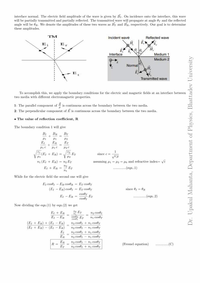
3.4.2 When the ~E is parallel to the plane of incidence: Transverse Magnetic

In order to derive this set of equation we will just use the principle of reversability of light. In such cases the angles will

straightway change from incident to refracted and vice versa. Also the boundary conditions for the electric field will now be the

boundary conditions for the magnetic and likewise for magnetic to electric.

To derive the Fresnel equations, consider two optical media separated by an interface, as shown in Fig. A planeoptical wave is propagating toward the interface with propagation vector ~κI oriented at angle θI with respect to the

Dr.


University

interface normal. The electric field amplitude of the wave is given by ~BI . On incidence onto the interface, this wavewill be partially transmitted and partially reflected. The transmitted wave will propagate at angle θT and the reflectedangle will be θR. We denote the amplitudes of these two waves as ~BT and ~BR, respectively. Our goal is to determinethese amplitudes.

To accomplish this, we apply the boundary conditions for the electric and magnetic fields at an interface betweentwo media with different electromagnetic properties.

1: The parallel component of~Bµ

is continuous across the boundary between the two media.

2: The perpendicular component of ~E is continuous across the boundary between the two media.

• The value of reflection coefficient, R


BI

µ1+

BR

µ1=

BT

µ2

EI

µ1 c+

ER

µ1 c=

ET

µ2 c√

ǫ1

µ1(EI + ER) =

√

ǫ2

µ2ET since c =

1√ǫ µ

n1 (EI + ER) = n2 ET assuming µ1 = µ2 = µ0 and refractive index=√ǫ

EI + ER =n2

n1ET ..............(eqn..1)

While for the electric field the second one will give

EI cosθI − ER cosθR = ET cosθT

(EI − ER) cosθI = ET cosθT since θI = θR

EI − ER =cosθT

cosθIET ..............(eqn..2)

Now dividing the eqn.(1) by eqn.(2) we get

EI + ER

EI − ER

=n2

n1

ET

cosθTcosθI

ET

=n2 cosθI

n1 cosθT

(EI + ER) + (EI − ER)

(EI + ER) − (EI − ER)=

n2 cosθI + n1 cosθT

n2 cosθI − n1 cosθT

EI

ER

=n2 cosθI + n1 cosθT

n2 cosθI − n1 cosθT

R =ER

ET

=n2 cosθI − n1 cosθT

n2 cosθI + n1 cosθT(Fresnel equation) ..............(C)

Dr.


University

• The value of transmission coefficient, T

Once this equation is derived you can start from anywhere from the continuity point of view. But I will start right from the scratch

since in your exam question may come asking to derive any one of them.

The boundary condition 1BI

µ1

+ BR

µ1

= BT

µ2

has lead us to the following simplification (see the last section)

BI

µ1+

BR

µ1=

BT

µ2

EI + ER =n2

n1ET

ER =n2

n1ET − EI ..............(eqn..1)

Now replacing the value of this ER in the eqn..(2) of the last section we will find

EI − ER =cosθT

cosθIET

EI − (n2

n1ET − EI) =

cosθT

cosθIET

2EI =

(

cosθT

cosθI+

n2

n1

)

ET

=

(

n1 cosθT + n2 cosθI

n1 cosθI

)

ET

T =ET

EI

=2n1 cosθI

n1 cosθT + n2 cosθI(Fresnel equation) ..............(D)

Key points to be taken away:

1. Both the coefficients (R & T) are independant of the material properties ie permittivity and permeability (asper the second form of the equations), though still have the implication of the refractive indices.

2. Both the coefficients (R & T) are only dependant on the angle of incidence θI and angle of refraction (transmission)θR(as per the both form of the equations).

Table 3.1: FRESNAL EQUATIONS

Co-efficients Transverse Electric Transverse Magnetic

R n1 cosθI −n2 cosθTn1 cosθI +n2 cosθT

n2 cosθI −n1 cosθTn2 cosθI +n1 cosθT

T 2n1 cosθIn1 cosθI +n2 cosθT

2n1 cosθIn1 cosθT +n2 cosθI

3.5 Brewster’s law

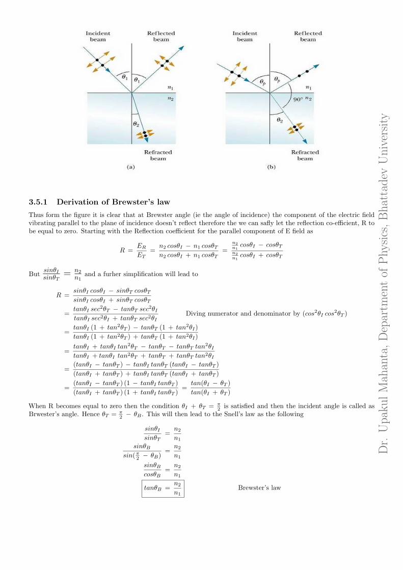
Brewsters law, relationship for light waves stating that the maximum polarization (vibration in one plane only) of a rayof light may be achieved by letting the ray fall on a surface of a transparent medium in such a way that the refractedray makes an angle of 90o with the reflected ray. The law is named after a Scottish physicist, Sir David Brewster, whofirst proposed it in 1811. To understand this let’s look at the following picture. A ray of ordinary (nonpolarized) lightof a given wavelength incident on a reflecting surface of a transparent medium (e.g., water or glass). Waves with theelectric field component vibrating in the plane of the surface are indicated by short lines crossing the ray, and thosevibrating at right angles to the surface, by dots. Most of the waves of the incident ray will be transmitted across theboundary (the surface of the water or glass) as a refracted ray making an angle r with the normal, the rest beingreflected (part (a) of the picture). But for a specific angle of incidence (p), called the polarizing angle or Brewstersangle, the electric field component vibrating at right angles to the surface vanishes completely (part (b) of the picture).

Dr.


University

3.5.1 Derivation of Brewster’s law

Thus form the figure it is clear that at Brewster angle (ie the angle of incidence) the component of the electric fieldvibrating parallel to the plane of incidence doesn’t reflect therefore the we can safly let the reflection co-efficient, R tobe equal to zero. Starting with the Reflection coefficient for the parallel component of E field as

R =ER

ET

=n2 cosθI − n1 cosθT

n2 cosθI + n1 cosθT=

n2

n1

cosθI − cosθTn2

n1

cosθI + cosθT

ButsinθIsinθT

= n2

n1and a furher simplification will lead to

R =sinθI cosθI − sinθT cosθT

sinθI cosθI + sinθT cosθT

=tanθI sec

2θT − tanθT sec2θI

tanθI sec2θI + tanθT sec2θIDiving numerator and denominator by (cos2θI cos

2θT )

=tanθI (1 + tan2θT ) − tanθT (1 + tan2θI)

tanθI (1 + tan2θT ) + tanθT (1 + tan2θI)

=tanθI + tanθI tan

2θT − tanθT − tanθT tan2θI

tanθI + tanθI tan2θT + tanθT + tanθT tan2θI

=(tanθI − tanθT ) − tanθI tanθT (tanθI − tanθT )

(tanθI + tanθT ) + tanθI tanθT (tanθI + tanθT )

=(tanθI − tanθT ) (1 − tanθI tanθT )

(tanθI + tanθT ) (1 + tanθI tanθT )=

tan(θI − θT )

tan(θI + θT )

When R becomes equal to zero then the condition θI + θT = π2 is satisfied and then the incident angle is called as

Brwester’s angle. Hence θT = π2 − θB . This will then lead to the Snell’s law as the following

sinθI

sinθT=

n2

n1

sinθB

sin(π2 − θB)=

n2

n1

sinθB

cosθB=

n2

n1

tanθB =n2

n1Brewster’s law

Dr.


University

3.6 Polarization of EM wave

Until now it seems that to describe light one must specify its frequency, its direction of propagation. But that’s onlytwo the third of complete description of the wave. In order to have the complete description one also must includeand its state of polarization. It’s must like a property of one-sidedness. The physical definition of wave polarizationis actually the time behaviour of the electric field of a Transverse EM wave at a given point in space. In other words,the state of polarization of a wave is described by the geometrical shape which the tip of the electric field vector drawsas a function of time at a given point in space. The plane in which the electric field oscillates is defined as the planeof polarization. Thus, polarization is a fundamental characteristic of a wave, and every wave has a definite state ofpolarization.So let us assume that we have monochromatic light propagating along the +z direction. Light is a transverse elec-tromagnetic wave, the electric field is always perpendicular to the direction of propagation. Because the direction ofpropagation is along the +z axis, the electric field vector, ~E must lie in the plane formed by the x and y axes. Thiscan be expressed mathematically as follows:

~E (x, y, z, t) = ~Ex(z, t)i + ~Ey(z, t)j

The components of the electric field Ex and Ey do not depend on x and y because we assume that the wave is a planewave propagating along the +z direction. Let us now consider two waves with their electric fields oriented in anddirections respectively.

For the x axis oriented wave

~Ex = ~E0x sin(ω t − κ z)

For the y axis oriented wave

~Ey = ~E0y sin(ω t − κ z + δ)

where δ is the phase constant between the two waves and the amplitudes E0x and E0y are real constants. .

3.6.1 Linnear Polarization:

Suppose both ~Ex and ~Ey components which are in phase ie δ = 0 having different magnitudes. The magnitudes of~Ex and ~Ey reach their maximum and minimum values simultaneously as ~Ex and ~Ey are in phase. Without losinggenerality let us take z = 0 which will give

~Ex = ~E0x sin(ω t − κ z) .....(1) ~Ey = ~E0y sin(ω t − κ z) .....(2)

Now (1) divided by (2) will give

~Ex

~Ey

=~E0x

~E0y

~Ex =~E0x

~E0y

~Ey

So at any point on the positive z axis, the ratio of magnitudes both the components is constant. This is the equation

of a straight line with slope~E0x

~E0y. The tip of electric field vector therefore draws a straight line if δ = 0, irrespective of

the amplitudes of the two field components. This polarization is hence called the Linear Polarization or the waveis said to be linearly polarized.

3.6.2 Circular Polarization:

If the two planes ~Ex and ~Ey (which are orthogonally polarized) are of equal in amplitude ( ~E0x = ~E0y = ~E0) but has90o phase difference between them, then the resulting wave is circularly polarized. In such case at any instant of time,if the amplitude of the any one component is maximum, then other component amplitude becomes zero due to thephase difference. Thus the magnitude of the resultant vector ~E is constant at any instant of time, but the directionis the function of angle between the relative amplitudes of ~Ex and ~Ey at any instant.


= ~E0 sin(ω t − κ z) .....(1)

~Ey = ~E0y sin(ω t − κ z +π

2)

= ~E0 cos(ω t − κ z) .....(2)

Now squaring and adding the last two equations we get

~E2x + ~E2

y = ~E20

Dr.


University

If the resultant electric field ~Ex is projected on a plane perpendicular to the direction of propagation, then the locusof all such points is a circle (since the last equation is the equation of a circle centered at origin with radius ~E0) withthe center on the z- axis. The circular polarization can be divided into Left-circular and Right-circular polarization.

• Right circularly polarized:If δ = −π

2 then vector ~E rotates clockwise ie to our right hand, then it is called the RIGHT HANDED ROTA-TION and light is called right circularly polarized.

• Left circularly polarized:If δ = π

2 then vector ~E rotates anticlockwise ie to our left hand, then it is called the LEFT HANDED ROTATIONand light is called left circularly polarized.

3.6.3 Elliptical Polarization:

In most of the cases, the components of the wave have different amplitudes and are at different phase angles otherthan 90 degrees. This results the elliptical polarization. Consider that electric field has both components ~Ex and~Ey which are not equal in amplitude and are not in phase. As the wave propagates, the maximum and minimum

amplitude values of ~Ex and ~Ey not simultaneous and are occurring at different instants of the time. Thus the directionof resultant field vector varies with time.


= ~E0x sinω t at z=0

~Ex

~E0x

= sinω t .....(1)

~Ey = ~E0y sin(ω t − κ z + δ)

= ~E0y sin(ω t + δ) at z=0

~Ey

~E0y

= sin (ω t + δ)

= sinω t cos δ + cos ω t sin δ .....(2)

Now eliminating ω t from equation (2) we get

~Ey

~E0y

=~Ex

~E0x

cos δ +

√

1 −~E2x

~E20x

sin δ

~Ey

~E0y

−~Ex

~E0x

cos δ =

√

1 −~E2x

~E20x

sin δ

~E2y

~E20y

− 2 ~Ex~Ey cos δ

~E0x~E0y

+~E2x

~E20x

cos2 δ =

(

1 −~E2x

~E20x

)

sin2 δ by squaring

~E2y

~E20y

− 2 ~Ex~Ey cos δ

~E0x~E0y

+~E2x

~E20x

cos2 δ = sin2 δ

If the locus of the end points of the field vector ~E traced then one can observe that the ~E moves elliptically on theplane. Hence such wave is called as elliptically polarized.

Documents

emt - Bhattadev University