Essays on Two-Sided Markets and Venture Capitalist ... · competition between platforms with di erent business models that connect consumers and application developers. In the rst

Essays on Two-Sided Markets and

Venture Capitalist Compensation

Ph.D. Thesis in Economics

Keke Sun

International Doctorate in Economic Analysis

Departament d’Economia i d’Historia Economica

Universitat Autonoma de Barcelona

Supervior: Prof. Jacobus Petrus Maria Hurkens

(Sjaak Hurkens)

Cerdanyola del Valles, October 2015

游游游子子子吟吟吟—唐·孟郊

慈母手中线，游子身上衣。临行密密缝，意恐迟迟归。谁言寸草心，报得三春晖。

Acknowledgements

First of all, I thank Sjaak Hurkens for his guidance, supervision and patience. Withouthim this thesis would not have been possible.

Throughout the course of my graduate studies, I have had the privilege of working withand learning from many amazing people at the Autonoma. I give my heartfelt thanks toDavid Perez-Castrillo, Roberto Burguet, Xavier Martinez-Giralt and Pau Olivella for theirconstant support and discussions. There are no words to match my gratitude. I owe animmense debt of gratitude to Susanna Esteban for reaching out to me when I needed itmost. I also would like to thank Luca Gambetti, Miguel Angel Ballester, Francesc Obiols,Tomas Rodrıguez-Barraquer and other faculty members for their presence in this journey. Afinal word to appreciate all the help from Angels Lopez and Merce Vicente, without whichmy Ph.D. life would have been a mess.

My sincere gratitude goes to my previous and current friends and colleagues at IDEA forsharing this journey with me, Fran, Arnau, Ezgi, too numerous to mention every single oneof them. I thank Nuno Alvim for his idea, his work in the third chapter of this thesis, andfor being so understanding towards my procrastination problem. I also thank Edgardo Larafor the all the discussions and the Spanish translation of the thesis abstract.

Financial support from Spanish Ministerio de Economia y Competitividad through re-search project ECO2009-07958 is gratefully acknowledged.

Special thanks go to my friends Jing Xu and Haishan Yu for their friendship and advice onPh.D. life. To Dan Wu, Yike Li, Haoyi Wang, thank you all, I have enjoyed your companyfor the past 15 years.

Finally, I thank my parents for their unconditional love and support all these years. Theyhave always been my source of strength. I know I don’t get to say this often, so... MAMAAND PAPA, I LOVE YOU!!! This thesis is dedicated to you.

I give my thanks for all those moments, both good and bad. Above all, I thank everyonefor making sure I never felt alone.

Introduction

The first two chapters of this thesis are about two-sided markets. Two-sided marketsare economic platforms that bring two interdependent groups of users together and enablecertain interactions between them. The main characteristic of two-sided markets is theindirect network externalities where one group’s benefits of joining the platform dependson the number of users from the other group on the same platform. These two chaptersare inspired by casual observations from the smartphone operating system (OS) industry.Major platform sponsors, i.e. Apple and Google, have brought their previously successfulfirm recipes to this new industry; and this has a significant bearing on their current platformstrategies. Apple bundles its OS platform with the high-end in-house handset while Googleadopts the ad-sponsored business model, introducing adverts on consumers side and collectrevenues from developers and advertisers. The first two chapters study the duopolisticcompetition between platforms with different business models that connect consumers andapplication developers.

In the first chapter, I study the impact of pure bundling and the level of consumer in-formation about developer subscription prices on duopolistic platform competition. I findthat, in the presence of asymmetric network externalities, pure bundling emerges as a profit-maximizing strategy when platforms subsidize the low-externality side (consumers) and makeprofits on the high-externality side (developers). Bundling can be used as a tool to enhancethe ”divide-and-conquer” nature of platform’s pricing strategies, and is more effective instimulating consumer demand the larger proportion of informed consumers. I also find thatconsumer information intensifies price competition. Consequently, bundling and more con-sumer information improve consumer welfare, but bundling is less likely to emerge as thefraction of informed consumers increases.

In the second chapter, I study the platform’s choice of business model between the puresubscription-based and the hybrid ad-sponsored business models when facing a subscription-based rival. Under the hybrid ad-sponsored business model, the platform adjusts its con-sumer subscription price to compensate consumers for the disutility induced by advertising,affecting consumer and developer demands, hence platform profits. I find that, when con-sumers have increasing marginal disutility towards advertising, the ad-sponsored businessmodel is more profitable when facing a subscription-based rival, no matter whether plat-forms set the subscription prices simultaneously on both sides or set the subscription priceson developer’s side before consumer’s side. Consumers are better off when the platformchooses the hybrid ad-sponsored business model, and are worse off when both platforms setthe subscription prices on developer’s side before consumer’s side.

The third chapter of the thesis contributes to the literature on the venture capital limitedpartnership agreements. The invisible component of the venture capitalist (VC) compen-sation is the value-of-distribution rules that determine when the VC receives his share of

i

profits and often generate an interest-free loan between the limited partners (LPs) and theVC. This chapter explores how the distribution rules affect the VC’s incentives on the timingof starting and exit decision of investments. We provide the first-best outcomes where theroles of capital provider and decision makers coincide as a benchmark, then compare theinvestment decisions under different distribution rules with the first-best outcomes. Thedistribution rules we look into are the Escrow contract, the Return First contract and thePayback contract (Litvak, 2009). Under the Escrow contract, the VC’s share of profits goesto an escrow account when each investment is realized. The VC only receives payments atthe fund liquidation date and the interest of this account goes to the LPs, which generatesan interest-free loan from the VC to the LPs. Under the Return First contract, the VCreceives no distributions until the invested capital has been fully paid back to the LPs foreach investment. After this threshold, the VC can receive his share of the profits at eachexit date. There should be no interest-free loan between the two parties once the investedcapital is returned. Under the Payback contract, the VC receives his share of the revenues atthe investment exit date and pays back the invested capital back to the LPs when the fundliquidates. This type of contract generates an interest-free loan from the LPs to the VC. Theresults we find are the following. If there is only one project under consideration, both thefirst-best investment duration (given a certain level of the carried interest) and the startingdate can be attained under the Return First contract because there is no interest-free loanbetween the two parties. If there are two investment projects under consideration, fixingthe project that starts first to be normal, only the Escrow contract can restore the first-bestinvestment durations given a certain level of the carried interest for the VC, but not thefirst-best starting dates. The first-best starting dates are possible to be attained only underthe Payback contract. Our results indicate that, regarding the investment durations, usinga certain level of the carry can overcome the distortions induced by the interest-free loanfrom the VC to the LPs, but not the distortion induced by the fact that the VC does notreturn the invested capital at the exit date.

ii

Contents

1 Bundling, information and platform competition 11.1 Introduction . . . . . . . . . . . . . . . . . . . . . . . . . . . . . . . . . . . . 11.2 Relationship to the Literature . . . . . . . . . . . . . . . . . . . . . . . . . . 31.3 The Model . . . . . . . . . . . . . . . . . . . . . . . . . . . . . . . . . . . . . 5

1.3.1 Platforms . . . . . . . . . . . . . . . . . . . . . . . . . . . . . . . . . 51.3.2 Consumers . . . . . . . . . . . . . . . . . . . . . . . . . . . . . . . . . 61.3.3 Developers . . . . . . . . . . . . . . . . . . . . . . . . . . . . . . . . . 7

1.4 Platform Competition . . . . . . . . . . . . . . . . . . . . . . . . . . . . . . 91.4.1 Symmetric Competition . . . . . . . . . . . . . . . . . . . . . . . . . 91.4.2 Bundling . . . . . . . . . . . . . . . . . . . . . . . . . . . . . . . . . . 121.4.3 Welfare Analysis . . . . . . . . . . . . . . . . . . . . . . . . . . . . . 201.4.4 Tying . . . . . . . . . . . . . . . . . . . . . . . . . . . . . . . . . . . 21

1.5 Extension: Heterogeneous Consumer Valuation of the Handset . . . . . . . . 221.5.1 Tying . . . . . . . . . . . . . . . . . . . . . . . . . . . . . . . . . . . 26

1.6 Concluding Remarks . . . . . . . . . . . . . . . . . . . . . . . . . . . . . . . 28

Appendix 30

2 Hybrid ad-sponsored platform 402.1 Introduction . . . . . . . . . . . . . . . . . . . . . . . . . . . . . . . . . . . . 402.2 Relationship to the Literature . . . . . . . . . . . . . . . . . . . . . . . . . . 422.3 The Model . . . . . . . . . . . . . . . . . . . . . . . . . . . . . . . . . . . . . 43

2.3.1 The timing of the game . . . . . . . . . . . . . . . . . . . . . . . . . 432.3.2 Platforms . . . . . . . . . . . . . . . . . . . . . . . . . . . . . . . . . 442.3.3 Developers . . . . . . . . . . . . . . . . . . . . . . . . . . . . . . . . . 452.3.4 Consumers . . . . . . . . . . . . . . . . . . . . . . . . . . . . . . . . . 45

2.4 Platform Competition . . . . . . . . . . . . . . . . . . . . . . . . . . . . . . 462.4.1 Subscription-Based Business Model . . . . . . . . . . . . . . . . . . . 502.4.2 Ad-sponsored Business Model . . . . . . . . . . . . . . . . . . . . . . 51

iii

2.5 Extension: Sequential Price Setting . . . . . . . . . . . . . . . . . . . . . . . 542.5.1 Subscription-based Business Model . . . . . . . . . . . . . . . . . . . 552.5.2 Ad-sponsored Business Model . . . . . . . . . . . . . . . . . . . . . . 57

2.6 Conclusion . . . . . . . . . . . . . . . . . . . . . . . . . . . . . . . . . . . . . 60

Appendix 62

3 How venture capitalist compensation affects investment decisionsjoint with Nuno Alvim 723.1 Introduction . . . . . . . . . . . . . . . . . . . . . . . . . . . . . . . . . . . . 723.2 The Model . . . . . . . . . . . . . . . . . . . . . . . . . . . . . . . . . . . . . 753.3 First-best outcomes . . . . . . . . . . . . . . . . . . . . . . . . . . . . . . . . 77

3.3.1 One Project . . . . . . . . . . . . . . . . . . . . . . . . . . . . . . . . 773.4 Contracts . . . . . . . . . . . . . . . . . . . . . . . . . . . . . . . . . . . . . 81

3.4.1 One Project . . . . . . . . . . . . . . . . . . . . . . . . . . . . . . . . 813.4.2 Two Projects . . . . . . . . . . . . . . . . . . . . . . . . . . . . . . . 87

3.5 Conclusion . . . . . . . . . . . . . . . . . . . . . . . . . . . . . . . . . . . . . 98

Appendix 100

References 107

iv

List of Figures

1.1 Best response curves on consumer side under bundling . . . . . . . . . . . . 111.2 Platform profits as functions of the level of consumer information . . . . . . 141.3 The impact of bundling on platform profits . . . . . . . . . . . . . . . . . . . 191.4 The impact of consumer information on bundling strategy . . . . . . . . . . 201.5 Consumers are heterogeneous with repsect to the valuation of the handset . 231.6 Bundling strategy when consumers are homogeneous and heterogeneous with

respect to the valuation handset . . . . . . . . . . . . . . . . . . . . . . . . . 251.7 Tying when consumers are heterogeneous w.r.t. the valuation of the handset 27

2.1 The differences on platform profits due to the order of the price setting asfunctions of θ (Scenario 2′−Scenario 2). . . . . . . . . . . . . . . . . . . . . 59

v

List of Tables

2.1 Subscription prices on two sides of Scenario 1 . . . . . . . . . . . . . . . . . 512.2 Changes in equilibrium outcomes due to advertising (Scenario 2−Scenario 1) 532.3 Subscription prices on two sides of Scenario 1′ . . . . . . . . . . . . . . . . . 562.4 Changes in equilibrium outcomes due to the order of price setting (Scenario

1′−Scenario 1) . . . . . . . . . . . . . . . . . . . . . . . . . . . . . . . . . . 572.5 Changes in equilibrium outcomes due to the order of price setting (Scenario

2′−Scenario 2) . . . . . . . . . . . . . . . . . . . . . . . . . . . . . . . . . . 58

3.1 Starting decision of project A . . . . . . . . . . . . . . . . . . . . . . . . . . 953.2 Starting decision of project A . . . . . . . . . . . . . . . . . . . . . . . . . . 97

vi

Chapter 1

Bundling, information and platformcompetition

1.1 Introduction

A smartphone operating system (OS) platform accommodates applications and makes theinteractions between consumers and application developers possible. This paper is motivatedby the phenomenal growth in the smartphone industry. As in other two-sided industries,an important decision for firms, with consequences for competition and welfare, is whetherto bundle the operating system with the hardware. Apple is currently a major competitorboth in the smartphone and the OS markets and its success in hardware has a significantbearing on its success in this industry (Kenney and Pon, 2011). Bundling with a best-sellinghandset certainly adds to the platform’s appeal for consumers1. Such bundling practice isalso common in industries like the video game industry, where major competitors like Sonyand Microsoft bundle the OS platforms with their in-house consoles.

In this paper, we emphasize yet another characteristic of these industries: asymmetryof information of the different players. Developers are industry-insiders; they are usuallyinformed about all subscription prices and have good predictions of participation decisionson both sides of the platform. In contrast, not every consumer knows the fixed fees orroyalties that the platforms charge to developers. Similarly, newspaper readers may not beaware of how much the newspaper charges advertisers for listing ads.

1The iPhone has been the top-selling mobile phone in the U.S. Source: http://www.bizjournals.com/

boston/blog/mass_roundup/2013/02/apple-top-selling-us-mobile-phone.html, accessed September,2014.

1

http://www.bizjournals.com/boston/blog/mass_roundup/2013/02/apple-top-selling-us-mobile-phone.html

http://www.bizjournals.com/boston/blog/mass_roundup/2013/02/apple-top-selling-us-mobile-phone.html

The goal of this work is to develop a theoretical model to analyze the bundling strategyfor platforms when information may be less than perfect for some users on different sidesof the platform. We address two main research questions. First, when does a platformpractice bundling as a profitable entry accommodation strategy? Second, how does the levelof consumer information affect platform competition and the bundling decision?

We consider a two-stage game in which one of the platforms makes a strategic decision,namely, whether to bundle with an in-house handset, in addition to competing through ad-justment of tactical variables which are subscription prices. In the first stage, this platformdecides whether to bundle with its in-house handset2, laying the groundwork for the compet-itive interactions down the line. In the second stage, the platforms decide subscription pricessimultaneously, and competition takes place. We do not consider bundling to be an act ofpredation, but rather a commitment to an aggressive pricing strategy. The platform sellsthe bundle at a discount, relative to separate selling, to stimulate consumer and developerdemand.

Within the framework of the Hotelling model, two platforms compete for single-homingconsumers and multi-homing developers. Departing from the standard setting of full in-formation and responsive expectations for all users in the two-sided markets literature, weassume that some consumers are uninformed about developer subscription prices and holdpassive expectations about developer participation, whereas the remaining consumers and alldevelopers are informed about all subscription prices and hold responsive expectations.

We find that, in the presence of asymmetric network externalities, price competition canlead to consumer prices being strategic substitutes when platform preferences are smallrelative to the benefits of attracting an additional consumer. Therefore, bundling, as a com-mitment to an aggressive pricing strategy, may be in the interest of the firm and detrimentalto the rival when platforms subsidize the low-externality side (consumers) and make profitson the high-externality side (developers). Bundling can be used as a tool to enhance the”divide-and-conquer” nature of the pricing strategies. When consumers are heterogeneouswith respect to the valuation of the handset, bundling can also emerge when consumer pricesare strategic complements, even though there is no subsidy for participation. Bundling ex-pands consumer demand for platform adoption as well as for the handset. Through bundling,the platform coordinates the misaligned consumer valuations of the platform and the hand-set, attracting consumers with a high valuation of the handset. Our results further showthat bundling improves consumer welfare by lowering the prices and offering more applicationvariety for the majority of consumers.

Our second set of findings concerns consumer information. We find that, when the frac-

2We consider pure bundling. Under pure bundling, the handset and the access to platform A can onlybe purchased as a bundle.

2

tion of informed consumers is larger, price competition is more intense. Informed consumersrespond to price changes by adjusting their demand and their expectations of developer de-mands accordingly. Therefore, bundling, deployed as an implicit discount on the consumersubscription price, is more effective to stimulate consumer demand when there are more ”re-sponsive” consumers. Consequently, the developer demand is also stimulated through thedemand shifting effect. Consumer surplus increases in the fraction of informed consumers,because a larger fraction of informed consumer leads to lower subscription prices and moreapplication variety. Consumer information also has a negative impact on the emergence ofbundling: the region in which bundling emerges shrinks as the fraction of informed consumersincreases. This is because bundling only emerges when the competing platform increases itsconsumer price in response to bundling, but more consumer information intensifies compe-tition and pushes the competing platform to be more aggressive.

The remainder of the paper is organized as follows. Section 1.2 briefly discusses the re-lated literature. In Section 1.3, we set up the duopoly model of platform competition. InSection 1.4, we investigate the bundling strategy of the platform when consumers are homo-geneous with respect to the valuation of the handset. We compare two scenarios, dependingon whether the platform practices or does not practice bundling. Section 1.5 studies thebundling strategy when consumers are heterogeneous with respect to the valuation of thehandset. Section 1.6 concludes.

1.2 Relationship to the Literature

This work contributes to the literature on two-sided platforms. A large share of this lit-erature studies pricing in the presence of network effects3. The literature shows that thestructure of equilibrium prices depends on the relative size of demand elasticities and indi-rect network externalities on each side, the marginal costs of serving each side, whether themarket structure has single-homing users on each side or takes the form of a competitivebottleneck, that is having single-homing users on one side and multi-homing users on theother side. This works studies the impact of bundling in the framework of two-sided plat-forms. Pure bundling is usually considered as an act of predation. Whinston (1990) showsthat pure bundling reduces equilibrium profits of all firms; hence, it is usually adopted todeter entry or drive the rival out of the market. However, in two-sided markets, this maynot be the case. Our paper fits this theme by considering bundling as a tool to stimu-late consumer demand. The present work is closely related to Farhi and Hagiu (2008) andAmelio and Jullien (2012). The former study shows that a subsidy on one side may lead

3See Caillaud and Jullien (2003), Rochet and Tirole (2003, 2006), Armstrong (2006), Armstrong andWright (2007), Hagiu (2006), Weyl (2010).

3

to fundamentally new strategic configurations in oligopoly. Farhi and Hagiu (2008) presentthe conditions upon which a cost-reducing investment by intermediaries may be a successfulentry accommodation strategy and may also benefit its rival. A possible interpretation isthat this reduction results from a tying strategy. Prices are not necessarily strategic com-plements in competition, the effects of cost-reducing investments on prices are ambiguousand platforms may earn negative margin on one side. Amelio and Jullien (2012) investi-gate the effects of tying of independent goods, with single-homing users on both sides ofthe platform. With a non-negativity constraint, tying works as an implicit subsidy. In themonopoly case, the platform prefers tying as it is a way to subsidize users that have lownetwork externality. Tying leads to higher participation, higher consumer surplus as well asprofits. In the duopoly case, tying on one side makes a platform more or less competitiveon the other side depending on externalities of the two sides. The impact of tying on plat-forms’ profits also depends on the relative levels of externalities. Total consumer surplusincreases in case of high asymmetry in the network externalities between two sides. Tyingis used to implement second-degree price discrimination to help a network to coordinate thecustomers’ participation. In Amelio and Jullien (2012), pure bundling arises if the value ofthe good is below its cost so that selling the good alone is not profitable. In this work, weshow that pure bundling works as a commitment device to allow the platform to be moreaggressive. The key features differentiating our work from this line of literature are: firstly,we study the effect of information asymmetry, namely, the level of consumer information, onplatform’s bundling strategy; secondly, we allow consumers to be heterogeneous with respectto the valuation of the handset. We believe that these features bring our analysis closer toreality. Using the one side single-homing and one side multi-homing, we show that bundlingalways hurt the rival, which differs from Farhi and Hagiu (2008) and Amelio and Jullien(2012). We also show that without the non-negativity constraint, tying makes no differencefrom untying when consumers have the homogeneous valuation of the handset tied and theconsumer market is fixed-sized.

Our work is also about information asymmetry across the two sides of the platform. Themain characteristic of two-sided platforms is the bilateral indirect network externalities whereone group’s benefit from joining the platform depends on the size of the other group thatjoins the same platform, which gives rise to a ”chicken-and-egg” problem (Armstrong, 2006;Hagiu, 2006). The majority of the existing literature on two-sided platform pricing assumesthat all users have full information about all prices and preferences, which implies that allusers can perfectly predict other’s participation decision. In reality, platform users, especiallyconsumers, may not be able to observe all prices or perfectly anticipate the impact of pricechanges on demands. Hurkens and Lopez (2014) suggest that passive expectation should be aplausible alternative for responsive expectation in a market with (direct or indirect) networkexternalities. Passive expectations, first introduced by Katz and Shapiro (1985), are fulfilledin equilibrium. Consumers with passive expectations use price information on consumer’s

4

side to fixate their expectation of developer demand and do not respond to any price changeson the other side of the platform. In the present work, we allow users on the two sides tohave different levels of information. We assume developers are always well-informed; theyare informed about all prices and hold responsive expectations about consumer participa-tion. Consumers are not necessarily as well-informed as developers, not every consumer isaware of how much the platforms charge developers for listing their applications. Therefore,we assume there is a fraction of consumers who are informed about developer prices andhold responsive expectations about developer participation while the remaining consumersare uninformed and hold passive expectations. In this spirit, the present paper is very closeto Hagiu and Ha laburda (2014). They study the effect of different levels of informationon two-sided platform profits, under both monopoly and competition. They assume thatdevelopers always hold responsive expectations while all users hold passive or responsive ex-pectations. They show that responsive expectation amplifies the effect of price reductions. Amonopoly platform can exploit the demand increases due to user’s responsive expectation, soit prefers facing more informed users. While more information intensifies price competition,competing platforms are affected negatively when users are well informed. Our symmetriccompetition subgame is a replica of Hagiu and Ha laburda (2014)’s hybrid scenario in whichsome consumers are informed while others are uninformed and hold passive expectations.We reach the same conclusion that more information intensifies price competition regardlessof the bundling decision. There is one key difference between Hagiu and Ha laburda (2014)and our analysis. They focus on the impact of different user expectations on equilibriumallocations in the context of monopoly and duopoly markets, whereas we are interested inthe impact of the level of consumer information on platform’s bundling decision in a duopolysetting, because our work models the competition between smartphone OS platforms wherebundling has a significant bearing.

1.3 The Model

1.3.1 Platforms

Consider two platforms competing for both consumers and developers, indexed by T=A,B. Let pCT and pDT denote the subscription prices platform T charges to consumers anddevelopers, respectively. We assume that the platforms have zero marginal cost of servingthese two groups of users, which is consistent with the literature of information goods andthe reality of digital media industry, where large fixed costs and very low marginal costs are

5

observed4. We allow for negative prices, as it is possible for platforms to subsidize one side ofthe market. The number of consumers and developers on platform T are denoted by nCT andnDT , respectively. We allow single-homing on one side and multi-homing on the other side.To be more specific, we assume that each consumer decides in favor of only one platformwhile developers can design applications for both platforms.

We extend the standard Hotelling model by allowing the duopoly to serve two groups ofusers on each side of the market. The unit transportation cost for consumers towards eachend is t, which is the platform differentiation parameter. Platform A and B are exogenouslylocated at x = 0 and x = 1, respectively. Platform T ’s profit maximization problem is

maxpCT ,p

DT

πT = pCT nCT + pDT n

DT ,

where T = A,B.

We assume one of the platforms (without loss of generality, platform A) has a in-housekiller handset with quality z and marginal cost C, for instance, the iPhone by Apple. Forcalculation simplicity, we normalize this marginal cost C = 0. Platform A is a monopolistin the high-end handset market, which vertically differentiated from the other handsets.Platform A can decide whether to bundle with this handset or not.

1.3.2 Consumers

There is mass 1 of consumers uniformly distributed along the unit interval, each of whomchooses at most one platform to join. The consumers have identical intrinsic values of twoplatforms, equivalent to v, which is assumed to be large enough so that the whole marketis covered. Consumers have a taste for application variety. Every consumer’s utility ofparticipating on a platform depends on the total number of developers on the same platform.Consumers have identical utility gain from application variety; parameter θ is used to capturethis direction of network externalities. More specifically, the availability of each additionaldeveloper positively generates additional utility θ for consumers, i.e. θ>0. We ignore thepotential positive direct externalities among consumers5. The consumer who locates at xdecides joining platform A or B by comparing utilities v+θnD

e

A −pCA−tx from platform A andv+θnD

e

B −pCB− t(1−x) from platform B. Following Hagiu and Ha laburda (2014), we assumethere are two types of consumers: a fraction λ of consumers is informed about developer

4This assumption is made for calculation simplicity. Assuming platforms have the marginal cost of cC

and cD of serving consumer’s side and developer’s side complicates the calculations but do not change thequalitative results of the model.

5The potential positive externalities indicate that consumers may derive positive utilities from the numberof other consumers on the same platform.

6

subscription prices and holds responsive expectations about developer participation whenchoosing between two platforms, 0≤λ≤1. The expectations of these consumers match therealized developer demand, i.e., nD

e

T = nDT . The remaining fraction 1−λ of consumers isuninformed about developer prices and holds passive expectations. They do not adjusttheir expectation of developer demand in response to price changes on developer’s side6.Therefore, the realized consumer demand of each platform is

nCT =1

2+pC−T − pCT

2t+λθnDT − λθnD−T

2t+

(1− λ)θnDe

T − (1− λ)θnDe

−T

2t, (1.1)

where T = A,B.

For now, we assume consumers are homogeneous with respect to the valuation of thehandset; they have identical marginal utility of the quality of platform A’s in-house handsetφ=1, and each buys at most one copy.

1.3.3 Developers

There is mass 1 of potential developers; each developer lists one application on one platform.Assume that developers form responsive expectations of consumer demand. Developersare industry insiders, they are aware of consumer’s preference, thus, can perfectly predictconsumer participation. Developers differ in the cost of listing applications, denoted by y, andare uniformly distributed along the segment [0, 1]. Each developer gains additional utilityof β from each consumer who has access to its application. The revenue for a developerwho lists on platform T is given by βnCT when the number of consumers who participatein platform T is nCT . We assume all applications are independent of one another, so thepotential negative direct network externalities are ignored. The utility of developer y fromjoining platform T is

uDT = βnCT − pDT − y,

where T = A,B. We assume that developers can multi-home7 and there are no economiesof scope in multihoming. Therefore, the decision of joining a platform is independent of thejoining decision of the other platform. That is, a y-type developer will join platform T ifuDT (y) = βnCT − pDT − y≥0. So, the developer demand of each platform is

nDT = βnCT − pDT .6Hurkens and Lopez (2014) offers a clear illustration of the difference between passive and responsive

expectations.7Some recent survey shows that on average mobile developers use 2.6 mobile platforms (VisionMobile,

2013).

7

Developers care more about the network benefits of reaching out to the widest population ofconsumers than they do about the cost of multi-homing since there is no standalone value fordevelopers to join the platforms. We study a case of ”competitive bottlenecks” (Armstrong,2006): there is a high level of competition on consumer’s side, and platforms make low profitson this side, but there is no competition for providing applications to consumers.

We assume that the following conditions hold throughout this paper:Assumption A1. β > 2θ.

We assume developers care more about consumers than consumers do about developers.This level of asymmetry between the two directions of network effect guarantees the existenceof the situation where platforms engage in divide-and-conquer strategies.Assumption A2. t > t = β2

6+ θβ

6+ θ2λ

6+ θβλ

2.

With these two assumptions, the conditions for unique and stable equilibrium (t > β2

6+

θ2λ2

6+ 2θβλ

3) and second order condition (t > θβλ) are satisfied, and both platforms make

positive profits in equilibrium, so that they remain active in the market8.

As we are interested in the impact of bundling on platform competition, we assume plat-form A’s bundling decision cannot drive its rival out of the market:Assumption A3. 0 < z < z = 3t− 3t.

When z≥z, platform A would always bundle the platform with the handset to push therival out of the market.

The next condition rules out the corner solution that the developer demand for eachplatform is 1:Assumption A4. θ + β < 2.

We propose a two-stage game. The timing of the game is as follows: In Stage 1, platform Amakes the strategic decision whether to bundle with its in-house handset or not. The decisionis publicly observable. In Stage 2, two platforms simultaneously decide on subscription pricesfor consumers and developers, and competition takes place.

8Notice that β2

6 + θβ6 + θ2λ

6 + θβλ2 −(β

2

6 + θ2λ2

6 + 2θβλ3 ) = ( θβ6 + θ2λ

6 )(1−λ)≥0 and β2

6 + θβ6 + θ2λ

6 + θβλ2 −θβλ =

β2

6 + θβ6 + θ2λ

6 −θβλ2 ≥

β2λ6 + θβλ

6 + θ2λ6 + θβλ

2 = λ6 (β − θ)2≥0. Therefore, once Assumption A2 is satisfied,

both t > β2

6 + θ2λ2

6 + 2θβλ3 and t > θβλ hold.

8

1.4 Platform Competition

We analyze the bundling strategy of the platform by comparing the no bundling and bundlingscenarios. We also compare bundling with tying. The difference between pure bundling andtying is that, the tied good is still available on a stand-alone basis under tying, which meansthat, under tying, consumers on platform B can still purchase the handset (see Tirole,2005).

1.4.1 Symmetric Competition

We first derive the competition outcomes when platform A doesn’t bundle with its in-househandset as the benchmark case. Platforms engage in symmetric competition as they bothmake profits through subscription. Platform T ’s profit function is given by

maxpCT ,p

DT


DT ,

where T = A,B. Platform A also has revenue z stemming from the in-house handset.

A fraction λ of consumers is informed about all subscription prices; they make the partici-pation decision upon subscription prices for both consumers and developers. The remainingconsumers are only informed about prices on consumer’s side; they make the participationdecision upon consumer subscription prices and their expectations about developer partici-pation for each platform. Thus, the realized consumer demand for each platform is

nCT =1

2+pC−T − pCT2t− 2θβλ

+θ(1− λ)nD

e

T − θ(1− λ)nDe

−T

2t− 2θβλ+θλpD−T − θλpDT

2t− 2θβλ, (1.2)

where T = A,B.

Proposition 1. When two platforms engage in symmetric competition, the competition equi-librium outcomes are as follows:

pC∗

T = t− β2

4− 3θβλ

4, nC

∗

T =1

2,

pD∗

T =β

4− θλ

4, nD

∗

T =β

4+θλ

4,

π∗A =t

2− θ2λ2

16− 3θβλ

8− β2

16+ z,

and

π∗B =t

2− θ2λ2

16− 3θβλ

8− β2

16,

where T = A,B.

9

Proof. See Appendix.

The equilibrium consumer subscription price is the standard Hotelling price with zeromarginal cost (t) adjusted downwards by β2

4+ 3θβλ

4. The adjustment term, which measures

the benefits to the platform from attracting an additional consumer, can be decomposedinto two factors β(β

4+ 3θλ

4). The first factor β means the platform attracts β additional

developers when it has an additional consumer. The second factor β4

+ 3θλ4

is the profitthat the platform can earn from an additional developer. The additional developer paysa subscription price β

4− θλ

4to the platform, also attracts θλ informed consumers because

only informed consumers would adjust their expectations of developer demand according toprice changes. The platforms decide their pricing strategies on consumer’s side by comparingplatform preferences with the benefits of attracting one extra consumer. The larger networkexternalities (β and θ) are, the lower price is charged on the consumer’s side.

The equilibrium developer subscription price is the monopoly pricing β4

9 adjusted down-wards by θλ

4, where θλ

4is the extra benefit that an extra developer brings to the platform from

attracting informed consumers. When β is large, developers attach a high value to consumerparticipation, and platforms have incentives to lower consumer prices or even subsidize con-sumers for participation. So that the platforms can charge higher prices on developer’s side.The equilibrium developer price increases with developer’s network externalities. When θ islarge, consumers attach a high value to developer participation, and platforms have incen-tives to lower developer prices to encourage participation, the equilibrium developer pricedecreases with consumer’s network externalities.

Corollary 1. The subscription prices on both sides of the platform are negatively affectedby the fraction of informed consumers while developer participation is positively affected byit. The platform profits decrease in the fraction of informed consumers.

When informed consumers are offered a lower price, they anticipate that consumer demandwould increase and developer demand would increase accordingly. This intensifies pricecompetition (Hagiu and Ha laburda, 2014). Indeed, the intensity of competition increases inthe fraction of informed consumers.

9If all consumers are uninformed about developer subscription prices and hold passive expectations aboutdeveloper demand, platforms exploit monopoly power on developer’s side and charge developer subscriptionprice β

2 pCT , the equilibrium developer subscription price is β

4 .

10

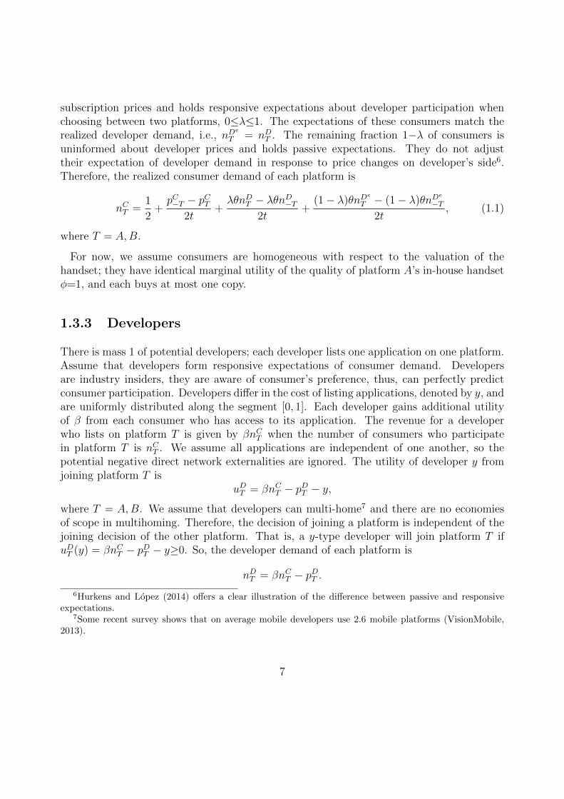
The best response function on consumer’s side is

pCT (pC−T ) =(4t− β2 − 3θβλ)(4t− θ2λ2 − 3θβλ)

γpC−T

+(4t− β2 − 3θβλ)(4t2 + θ2β2λ2 − 5tθβλ)

γ

+(4t− β2 − 3θβλ)θ(1− λ)(4t− 3θβλ)(nD

e

T − nDe

−T )

γ,

(1.3)

where γ = 32t2 − 4tθ2λ2 − 44tθβλ− 4tβ2 + 3θ3βλ3 + 14θ2β2λ2 + 3θβ3λ.

Depending on whether the platforms charge consumers positive prices or subsidize con-sumers for participation, we have two cases. When t > β2

4+ 3θβλ

4, the platforms charge

consumers positive prices for participation, this is the case where platform preferences arelarger than the benefits of attracting an extra consumer. The best response curves on con-sumer’s side are upward-sloping (see the dashed lines in Figure 1.1(a)), the consumer prices

of the two platforms are strategic complements (∂pCT (pC−T )

∂pC−T> 0). This is the case we often

see in one-sided market. When t < t < β2

4+ 3θβλ

4,platform preferences are small relative

to the benefits of attracting an extra consumer. This is the case where platforms subsidizeconsumers, which is the low-externality side, and earns a positive margin on developer’s side,which is the high-externality side. This is often seen in two-sided markets as the ”divide-and-conquer” strategy(Caillaud and Jullien, 2003). The best response curves on consumer’sside are downward-sloping (see the dashed lines in Figure 1.1(b)), and the consumer prices

are strategic substitutes (∂pCT (pC−T )

∂pC−T< 0) (Besanko et al., 2000).

0 pCA

pCB

RB

RA

(a) Strategic Complements

0pCA

pCB

RA

RB

(b) Strategic Substitutes

Figure 1.1: Best response curves on consumer side under bundling

11

1.4.2 Bundling

We assume platform A sets pA as the price for the bundled products, then pCA = pA − zis the implicit subscription price for consumers. Under pure bundling, neither the in-househandset nor the access to platform A would be available on a standalone basis. PlatformA would now charge a lower price for the bundled products, relative to separate selling.Under bundling, platform A has more incentives to lower the consumer price, a fall of pCA notonly encourages consumer participation, but also stimulates demand of the handset. Themarginal consumer locating at x derives utility v+ z− (pCA + z)− tx+ θnD

e

A from purchasingthe bundle and v − pCB − t(1 − x) + θnD

e

B from joining platform B. Again, a fraction λ ofconsumers is informed about developer subscription prices and holds responsive expectationsabout developer participation, i.e., nD

e

T = nDT ; while the remaining consumers are uninformedand hold passive expectations. Therefore, the consumer demand of each platform is the sameas Eq. (1.1). Platform A’s profit maximization problem evolves to

maxpCA,p

DA

πA = pAnCA + pDAn

DA = (pCA + z)nCA + pDAn

DA .

Platform B’s profit maximization problem is unchanged.

The following proposition characterizes the equilibrium prices and allocations in the bundlingscenario.

Proposition 2. When platform A bundles with its in-house handset and consumers arehomogeneous with respect to the valuation of the handset, the equilibrium outcomes are asfollows:

pC∗

A = t− β2

4− 3θβλ

4− z(8t− 2θβ − β2 − 2θ2λ− 3θβλ)

12(t− t),

pC∗

B = t− β2

4− 3θβλ

4− z(4t− β2 − 3θβλ)

12(t− t),

nC∗

A =1

2+

z

6(t− t), nC

∗

B =1

2− z

6(t− t),

pD∗

A = (β − θλ

2)(

1

2+

z

6(t− t)), nD

∗

A = (β + θλ

2)(

1

2+

z

6(t− t)),

pD∗

B = (β − θλ

2)(

1

2− z

6(t− t)), nD

∗

B = (β + θλ

2)(

1

2− z

6(t− t)),

π∗A =8t− β2 − θ2λ2 − 6θβλ

16

(6(t− t) + 2z)2

36(t− t)2

12

and

π∗B =8t− β2 − θ2λ2 − 6θβλ

16

(6(t− t)− 2z)2

36(t− t)2.


Under bundling, only consumers on platform A purchase the handset. Platform A hasto lower its consumer price to stimulate the demand for the bundled products. Thus, itmanages to steal some consumers from its rival. The higher value of the bundling handset,the more leverage platform A has on consumers. However, the cut on platform A’s consumerprice dominates the increment on its consumer demand. Hence, platform A suffers a loss onconsumer’s side. Yet, the direction of change on platform B’s consumer subscription priceis ambiguous, depending on the strategic relationship between consumer subscription prices.When consumer prices are strategic complements (resp. substitutes), platform B’s consumerprice goes down (resp. up). The directions of changes on profits from developer’s side forboth platforms are clear. As a fall on pCA shifts the consumer demand toward platformA, platform A (resp. B) becomes more (resp. less) attractive on developer’s side throughnetwork effects. This effect increases with β, which determines the sensitivity of developerdemand to the demand on consumer’s side.

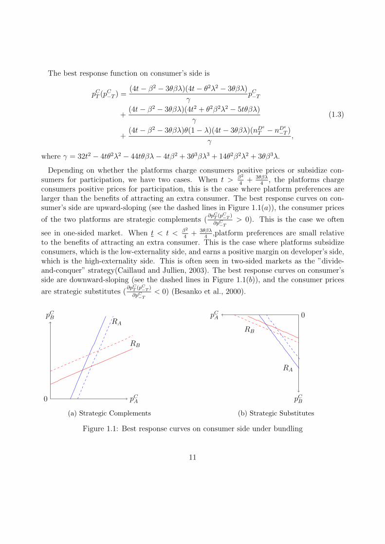
Corollary 2. When platform A bundles with its in-house handset, its implicit consumerprice decreases with the fraction of informed consumers while its demands on both sides ofthe platform increase with it. Platform B’s developer price, demands on both sides of theplatform and total profits are negatively affected by the fraction of informed consumers.

This corollary has significant empirical implications. It indicates that bundling is a moreeffective tool to stimulate consumer demand when there are more informed consumers. Theeffect of a discount on platform A’s consumer price is amplified. Platform A’s demands onboth sides of the market reach the highest levels when all consumers are informed. PlatformB suffers the largest loss when all consumers are informed. The effect of the fraction of theinformed consumers on platform A’s profits is ambiguous. Figure 1.2 illustrates how platformprofits under bundling change with the fraction of informed consumers λ, for certain valuesθ, β and z. All graphs have parameter t = 0.5. The solid line depicts πA and the dotted linedepicts πB.

13

(a) θ = 0.3, β = 0.7, z = 34(3t− 3t)

(b) θ = 0.2, β = 0.9, z = 34(3t− 3t)

(c) θ = 0.3, β = 0.7, z = 14(3t− 3t)

(d) θ = 0.2, β = 0.9, z = 14(3t− 3t)

Figure 1.2: Platform profits as functions of the level of consumer information

The system of best response functions on consumer’s side is as follows:

pCA(pCB) =(4t− β2 − 3θβλ)(4t− θ2λ2 − 3θβλ)

γpCB

+(4t− β2 − 3θβλ)(4t2 + θ2β2λ2 − 5tθβλ)

γ

+(4t− β2 − 3θβλ)θ(1− λ)(4t− 3θβλ)(nD

e

A − nDe

B )

γ

− 16t2 − 4tθ2λ2 − 20tθβλ+ 3θ3βλ3 + 5θ2β2λ2

γz,

(1.4)

14

and

pCB(pCA) =(4t− β2 − 3θβλ)(4t− θ2λ2 − 3θβλ)

γpCA

+(4t− β2 − 3θβλ)(4t2 + θ2β2λ2 − 5tθβλ)

γ

+(4t− β2 − 3θβλ)θ(1− λ)(4t− 3θβλ)(nD

e

B − nDe

A )

γ

− θ2λ2(4t− β2 − 3θβλ)

γz.

(1.5)

Compared to Eq. (1.3), there are two effects determining the movements of the best re-sponse curves. The terms proportional to z represent the impact of bundling on consumerprices. Bundling has a direct impact on consumer prices: all consumers observe the changeson consumer prices. It also has an indirect impact on consumer prices: informed consumersanticipate the impact of bundling on developer’s participation decisions. The terms propor-tional to nD

e

A − nDe

B represent the impact of bundling on perceived platform quality in termsof application variety for uninformed consumers. Following Amelio and Jullien (2012), weseparate the impact of pCA on the derivative of platform profits as follows:

∂

∂pCA(∂πA∂pDA

) =∂nCA∂pDA

+∂nDA∂pCA

= − θλ

2t− 2θβλ− β

2t− 2θβλ, (1.6)

and∂

∂pCA(∂πB∂pDB

) =∂nDB∂pCA

=β

2t− 2θβλ. (1.7)

The term − β2t−2θβλ

in Eq. (1.6) captures the fact that a fall of pCA shifts the consumerdemand towards platform A. As a result, platform A becomes more attractive for developers.The best response curve of platform A shifts upwards because its perceived quality hasimproved for consumers. Similarly, the term β

2t−2θβλin Eq. (1.7) indicates that a fall of pCA

makes platform B less attractive for developers.

The term− θλ2t−2θβλ

in Eq. (1.6) captures the other direction of the demand shifting effect. A

fall of pDA increases the developer demand for platform A, which improves platform quality interms of application variety. Therefore, the consumer demand shifts upwards. Note that thisdirection of effect is discounted because only informed consumers adjust their expectationsof developer demand according to the price change. The sensitivity of this direction ofdemand shifting effect depends on both consumer’s network externalities and the fraction ofinformed consumers. The higher fraction of informed consumers there is, the more sensitivethis direction of demand shifting effect is.

15

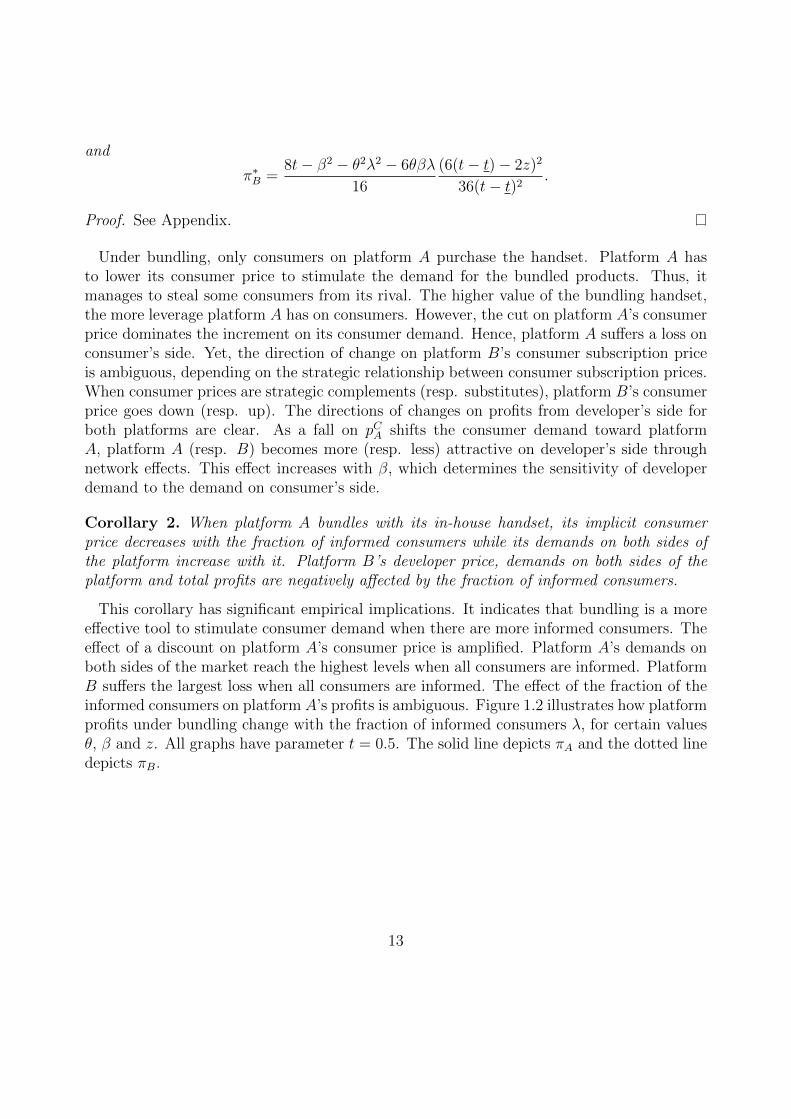
In the same fashion as before, we further discuss the impact of bundling decision depend-ing on whether the platforms charge consumers positive prices or subsidize consumers forparticipation.

1.4.2.1 Case I. Strategic Complements

When t > β2

4+ 3θβλ

4, the best response curves are again upward-sloping, indicating that the

consumer prices are strategic complements. The best response curves are shown in Figure1.1(a). Compare to the dashed lines in Figure 1.1(a), we see that, under bundling, theresponse curve of platform A moves to the left and the curve of platform B shifts downwards.Through bundling, platform A offers a discount on consumer subscription price, so theresponse curve of platform A moves downwards, but this effect is dampened by consumer’sexpectations of more application variety on platform A. Under bundling, platform A hasa higher consumer demand, the demand shifting effect indicates that it also has a higherdeveloper demand, the perceived quality of platform A increases and the perceived quality ofplatform B decreases. Platform A’s best response curve has the tendency to move upwards.Also, when consumer prices are strategic complements, platformB lowers its price in responseto bundling.

Pure bundling, works as a commitment device, has both a direct and a strategic effecton the platform’s profits (Besanko et al., 2000). The direct effect of the commitment isits impact on the platform profits if the rival’s behavior does not change, and the strategiceffect takes into account how the commitment changes the tactical decisions of rivals and,ultimately, the market equilibrium (Besanko et al., 2000). We decompose the effect of zon platform A’s own profits into a direct effect and strategic effects on both sides of theplatform.

dπAdz

=∂πA∂z

+∂πA∂pCB

dpC∗

B

dz+∂πA∂pDB

dpD∗

B

dz

Note that the direct effect is ∂πA∂z

= nCA. It indicates that platform A suffers a loss on the

handset sales under bundling compared to the no bundling case. The term ∂πA∂pCB

dpC∗

B

dzrepresents

the strategic effect of bundling on consumer’s side:

∂πA∂pCB

dpC∗

B

dz= (pCA + z + βpDA)

∂nCA∂pCB

(−4t− β2 − 3θβλ

12(t− t)) < 0.

The intuition is that bundling drives the rival to set the consumer price low when prices are

strategic complements, it intensifies competition on consumer’s side. The last term ∂πA∂pDB

dpD∗

B

dz

16

represents the strategic effect of bundling on developer’s side:

∂πA∂pDB

dpD∗

B

dz= (pCA + z + βpDA)

∂nCA∂pDB

(− β − θλ12(t− t)

) < 0.

Bundling has a strategic effect on developer’s side because informed consumers adjust theirexpectations about developer participation due to bundling. Bundling makes the competingplatform less attractive for developers through the demand shifting effect. Consequently,the competing platform has to lower its developer price. In this case, bundling intensifiescompetition on both sides of the platform. The speed of platform A’s profit increasing in thevalue of the handset drops from 1 (no bundling) to a speed slower than nCA (under bundling)(see Figure 1.3(a)). Bundling cannot be profitable for platform A in this case.

Bundling has strategic effects on platform B’s profits:

dπBdz

=∂πB∂pCA

dpC∗

A

dz+∂πB∂pDA

dpD∗

A

dz.

The first term of strategic effect also concerns the effect of bundling on consumer’s side:

∂πB∂pCA

dpC∗

A

dz= (pCB

∂nCB∂pCA

+ pDBβ∂nCB∂pCA

)(−8t− β2 − 2θβ − 2θ2λ− 3θβλ

12(t− t)) < 0.

Under bundling, platform A sets a low subscription price, platform B has to lower its pricein response. Platform A’s bundling decision leads to a more competitive environment onconsumer’s side. On developer’s side, the strategic effect of bundling is:

∂πB∂pDA

dpD∗

A

dz= (pCB

∂nCB∂pDA

+ pDBβ∂nCB∂pDA

)(β − θλ

12(t− t)) > 0.

Bundling makes platform A more attractive to developers, which increase its developer sub-scription price. Thus, there is room for platform B to increase its developer subscriptionprice as well. Bundling softens competition on this side of the platform. The over all effectof z on platform B’s profits are as follows:

dπBdz

= nCB(−8t− β2 − 2θβ − 2θ2λ− 3θβλ

12(t− t)) + θλnCB(

β − θλ12(t− t)

) < 0.

Bundling is detrimental to platform B’s profit in this case.

1.4.2.2 Case II. Divide-and-Conquer

When t < t < β2

4+ 3θβλ

4, the best response curves are downward-sloping and consumer

subscription prices are again strategic substitutes. Both platforms subsidize consumers for

17

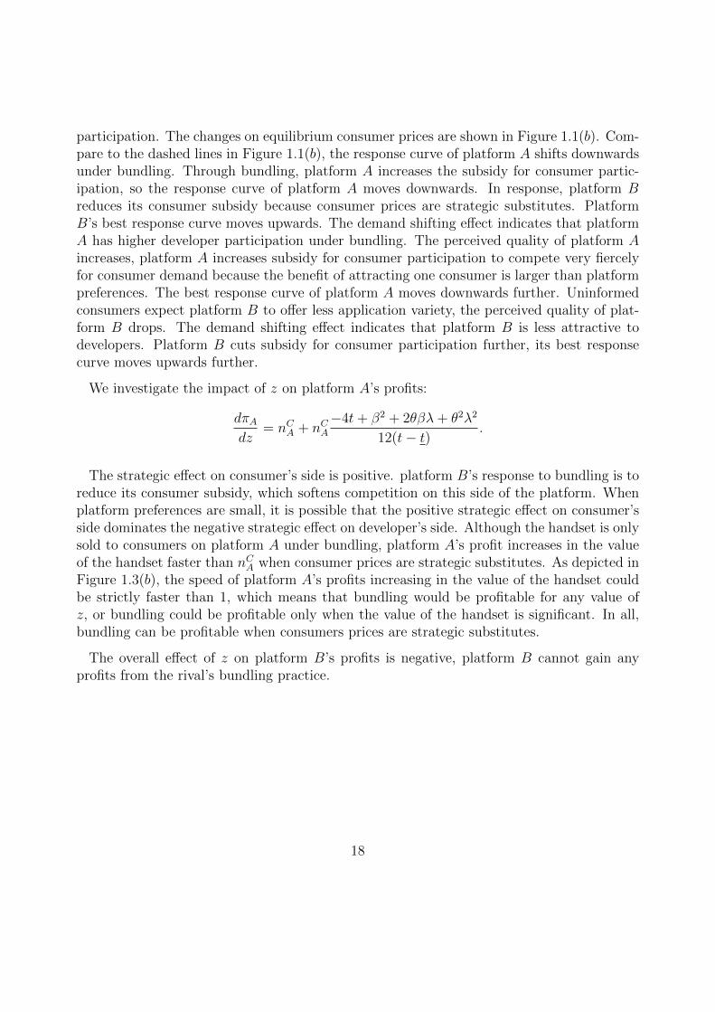
participation. The changes on equilibrium consumer prices are shown in Figure 1.1(b). Com-pare to the dashed lines in Figure 1.1(b), the response curve of platform A shifts downwardsunder bundling. Through bundling, platform A increases the subsidy for consumer partic-ipation, so the response curve of platform A moves downwards. In response, platform Breduces its consumer subsidy because consumer prices are strategic substitutes. PlatformB’s best response curve moves upwards. The demand shifting effect indicates that platformA has higher developer participation under bundling. The perceived quality of platform Aincreases, platform A increases subsidy for consumer participation to compete very fiercelyfor consumer demand because the benefit of attracting one consumer is larger than platformpreferences. The best response curve of platform A moves downwards further. Uninformedconsumers expect platform B to offer less application variety, the perceived quality of plat-form B drops. The demand shifting effect indicates that platform B is less attractive todevelopers. Platform B cuts subsidy for consumer participation further, its best responsecurve moves upwards further.

We investigate the impact of z on platform A’s profits:

dπAdz

= nCA + nCA−4t+ β2 + 2θβλ+ θ2λ2

12(t− t).

The strategic effect on consumer’s side is positive. platform B’s response to bundling is toreduce its consumer subsidy, which softens competition on this side of the platform. Whenplatform preferences are small, it is possible that the positive strategic effect on consumer’sside dominates the negative strategic effect on developer’s side. Although the handset is onlysold to consumers on platform A under bundling, platform A’s profit increases in the valueof the handset faster than nCA when consumer prices are strategic substitutes. As depicted inFigure 1.3(b), the speed of platform A’s profits increasing in the value of the handset couldbe strictly faster than 1, which means that bundling would be profitable for any value ofz, or bundling could be profitable only when the value of the handset is significant. In all,bundling can be profitable when consumers prices are strategic substitutes.

The overall effect of z on platform B’s profits is negative, platform B cannot gain anyprofits from the rival’s bundling practice.

18

0 z

π

Bundling

NB

(a) Strategic Complements

0 z

π

Bundling

NB

(b) Strategic Substitutes

Figure 1.3: The impact of bundling on platform profits

Platform A determines its bundling strategy by comparing the profits in two subgames. Let

t1 = 3β2+4θβ+6θβλ+4θ2λ−θ2λ216

, z1 = (6t−6t)(16t+θ2λ2−4θ2λ−6θβλ−4θβ−3β2)8t−θ2λ2−6θβλ−β2 and t2 = 5β2+8θβ+6θβλ+8θ2λ−3θ2λ2

24.

The following proposition states platform A’s bundling strategy.

Proposition 3. When consumers are homogeneous with respect to the valuation of platformA’s in-house handset,(i) platform A always chooses to bundle with the handset for all z < z when t < t≤t1;(ii) platform A bundles if the value of the handset is high, i.e., z1≤z < z, when t1 < t≤t2;(iii) platform A never practices bundling when t > t2,Bundling always hurts the rival.


It is worth commenting that when platform preferences are small relative to the networkexternalities, a small extra consumer demand can lead to significant profits on developer’sside, so platform A is willing to bundle with the handset even if it can only steal smallconsumer demand from the rival. When the platform preferences are medium, to recoup theloss on consumer’s side due to bundling, platform A needs to have a great consumer demand.Therefore, platformA would practice bundling only when bundling can steal a large consumerdemand from the rival, that is to say, the value of bundled handset needs to be significant.When platform preferences are large relative to the network externalities, platform A cannever recoup the loss on consumer’s side given a fixed-sized consumer market; bundlingnever occurs. Bundling works as a commitment to an aggressive pricing strategy and it onlyemergence when platforms subsidize consumers for participation, therefore, bundling can beused as tool to enhance the ”divide-and-conquer” nature of the pricing strategies.

19

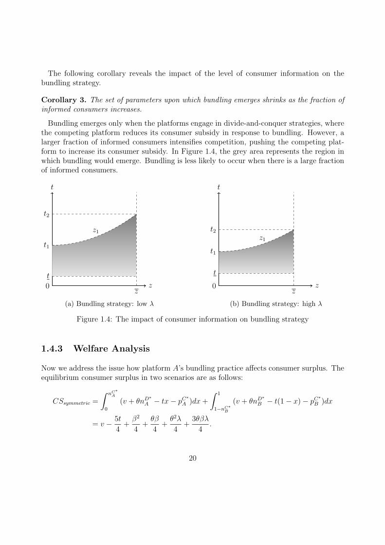
The following corollary reveals the impact of the level of consumer information on thebundling strategy.

Corollary 3. The set of parameters upon which bundling emerges shrinks as the fraction ofinformed consumers increases.

Bundling emerges only when the platforms engage in divide-and-conquer strategies, wherethe competing platform reduces its consumer subsidy in response to bundling. However, alarger fraction of informed consumers intensifies competition, pushing the competing plat-form to increase its consumer subsidy. In Figure 1.4, the grey area represents the region inwhich bundling would emerge. Bundling is less likely to occur when there is a large fractionof informed consumers.

t

0 zt

t1

t2

z1

z

(a) Bundling strategy: low λ

t

0 z

t1

t

t2z1

z

(b) Bundling strategy: high λ

Figure 1.4: The impact of consumer information on bundling strategy

1.4.3 Welfare Analysis

Now we address the issue how platform A’s bundling practice affects consumer surplus. Theequilibrium consumer surplus in two scenarios are as follows:

CSsymmetric =

∫ nC∗A

0

(v + θnD∗

A − tx− pC∗

A )dx+

∫ 1

1−nC∗B

(v + θnD∗

B − t(1− x)− pC∗B )dx

= v − 5t

4+β2

4+θβ

4+θ2λ

4+

3θβλ

4.

20

CSbundling =

∫ nC∗A

0

(v + θnD∗

A − tx+ z − z − pC∗A )dx+

∫ 1

1−nC∗B

(v + θnD∗

B − t(1− x)− pC∗B )dx

= v − 5t

4+β2

4+θβ

4+θ2λ

4+

3θβλ

4+z

2+

tz2

(6t− 6t)2

Corollary 4. Consumer surplus is positively affected by the fraction of informed consumers.Under bundling, consumer surplus is positively affected by the value of the handset.

A higher level of consumer information leads to lower subscription prices and higher devel-oper participation, resulting in greater consumer surplus. Also, both consumer and developerparticipation on platform A is positively affected by the value of the bundling handset whileplatform A’s consumer subscription price is negatively affected. The surplus of the major-ity of consumers increases with the value of the handset. Therefore, in general, consumersurplus increases with it.

Bundling has indeed one negative and two positive effects on consumer welfare. On theone hand, the unequal-split of consumer demand between two platforms increases totaltransportation cost, which reduces consumer welfare. The larger the difference in consumerdemand between the two platforms, the larger adverse welfare effect of bundling. On theother hand, there are two positive welfare effects of bundling coming from the fact thatthe majority of consumers enjoy a lower subscription price and more application variety,which dominates the negative effect on consumer surplus caused by lower subsidy and lessapplication variety for consumers on platform B. The change on consumer surplus due toplatform A’s bundling decision is

∆CS = CSbundling − CSsymmetric

=z

2+

tz2

(6t− 6t)2> 0

Proposition 4. When consumers are homogeneous with respect to the valuation of thebundling handset, platform A’s bundling decision unambiguously improves consumer wel-fare.

1.4.4 Tying

If platform A practices tying, it still sells the handset to consumers on platform B andextracts full surplus of the handset from them. Platform A’s maximization problem nowevolves to

maxpCA,p

DA

πA = (pCA + z)nCA + pDAnDA + nCBz = pCAn

CA + pDAn

DA + z.

21

Proposition 5. When consumers are homogeneous with respect to the valuation of platformA’s in-house handset and platform A extracts full surplus from the fixed-sized handset market,tying makes no difference from untying.

1.5 Extension: Heterogeneous Consumer Valuation of

the Handset

Now we modify our setting regarding consumer’s valuation of the handset. Let consumer’slocation on the unit interval be x and the marginal utility of the quality of platform A’s in-house handset be φ. The pair (x, φ) defines a consumer type. Both x and φ are distributedindependently and uniformly on [0, 1]. Type-φ consumer’s utility from the handset is

Uhs = φz − phs.

Without bundling, platform A sells the handset at monopoly price phs = z2, and the demand

for this handset is D(phs) = 12. Consumers with high marginal utility φ≥φ = 1

2purchase

(Figure 1.5(a)). Platform A earns revenue πhs = z4

from the unbundled handset.

Again, we assume platform A sets pA as the price for the bundled products, where pA =pCA + z

2. Consumers with the heterogeneous marginal utility of the handset quality derive

different levels of utility from purchasing the bundled products (Figure 1.5(b)). For instance,consumer (x, 0) derives utility v− pA + θnD

e

A − tx from purchasing the bundle and v− pCB +θnD

e

B − t(1− x) from joining platform B, the marginal consumer with 0 marginal utility forthe handset quality is

x0 =1

2+pCB − pCA

2t− z

4t+λθnD

e

A − λθnDe

B

2t+

(1− λ)θnDe

A − (1− λ)θnDe

B

2t.

Similarly, consumer (x, 1) derives utility v− pA + z + θnDe

A − tx from purchasing the bundleand v−pCB+θnD

e

B −t(1−x) from joining platform B, the marginal consumer with the highestmarginal utility of the handset quality is

x1 =1

2+pCB − pCA

2t+z

4t+λθnD

e

A − λθnDe

B

2t+

(1− λ)θnDe


B

2t.

The realized consumer demand of each platform is the same as Eq. (1.1).

22

0B

1

A+ hs

A B

B + hs

A

1

x

φ = 12

(a) No Bundling

0B

1

A

1

Bbundle

x0

x1

(b) Bundling

Figure 1.5: Consumers are heterogeneous with repsect to the valuation of the handset

Platform A’s profit maximization problem evolves to

maxpCA,p

DA

πA = pAnCA + pDAn

DA = (pCA +

z

2)nCA + pDAn

DA .

Proposition 6. When platform A bundles with its in-house handset and consumer’s marginalutility of the handset quality is uniformly distributed over [0, 1], the equilibrium outcomes areas follows:

pC∗

A = t− β2

4− 3θβλ

4− z(8t− 2θβ − β2 − 2θ2λ− 3θβλ)

24(t− t),

pC∗

B = t− β2

4− 3θβλ

4− z(4t− β2 − 3θβλ)

24(t− t),

nC∗

A =1

2+

z

12(t− t), nC

∗

B =1

2− z

12(t− t),

pD∗

A =β − θλ

2(1

2+

z

12(t− t)), nD

∗

A =β + θλ

2(1

2+

z

12(t− t)),

pD∗

B =β − θλ

2(1

2− z

12(t− t)), nD

∗

B =β + θλ

2(1

2− z

12(t− t)),

π∗A =8t− β2 − θ2λ2 − 6θβλ

16

(6t− 6t+ z)2

(6t− 6t)2,

and

π∗B =8t− β2 − θ2λ2 − 6θβλ

16

(6t− 6t− z)2

(6t− 6t)2.

23


Let t3 = 2θβ+β2+2θ2λ−θ2λ24

, z2 = (6t−6t)(8t−4θβ−2β2−4θ2λ+2θ2λ2)8t−β2−θ2λ2−6θβλ

and t4 = 8θβ+3β2+8θ2λ−5θ2λ2−6θβλ8

.We use the following proposition to identify the bundling strategy for platform A when con-sumer’s valuation of the handset is uniformly distributed along [0, 1].

Proposition 7. When consumer’s marginal utility of the quality of platform A’s in-househandset is uniformly distributed over [0, 1],(i) platform A chooses to bundle with the handset for all z < z when t < t≤t3;(ii) platform A practices bundling iff z2≤z < z when t3 < t≤t4;(iii) platform A never practices bundling when t > t4,Bundling always hurts the rival.


The set of parameters upon which bundling emerges is strictly larger than the case whereconsumers are homogeneous with respect to the valuation of the handset. Again, the setof parameters upon which bundling emerges shrinks as the fraction of informed consumersincreases. Notice that bundling can be profitable even when consumer subscription prices arestrategic complements. When all consumers are uninformed and hold passive expectations,bundling can be profitable even when consumer subscription prices are strategic complementsregardless of the value of the handset. We compare the regions in which bundling emergeswhen consumers are homogeneous or heterogeneous with respect to the valuation of thehandset (see Figure 1.6).

24

t

0 zt

β2

4+ 3θβλ

4

t1

t2

z1

z

(a) homogeneous valuation of the handset

t

0 z

t3

t

t4

β2

4+ 3θβλ

4

z2

z

(b) heterogeneous valuation of the handset

Figure 1.6: Bundling strategy when consumers are homogeneous and heterogeneous withrespect to the valuation handset

Indeed, the overall effect of z on platform A’s profit is:

dπAdz

= nCA + (pCA +z

2+ βpDA)

∂nCA∂pCB

(−4t− β2 − 3θβλ

12(t− t)) + (pCA +

z

2+ βpDA)

∂nCA∂pDB

(− β − θλ24(t− t)

).

When consumer prices are strategic substitutes, the strategic effects are positive, dπAdz

> nCA,platform A’s profit increases in value of the handset at a rate faster than nCA, also bundlingexpands consumer demand (nCA > 1

2), bundling is profitable. When consumer prices are

strategic complements, although platform A’s profit increases in value of the handset at arate slower than nCA, given the expanded consumer demand for the bundle, bundling still canbe profitable.

From Figure 1.5(b), we see a difference in consumer demand between consumers with ahigh valuation of the handset and the ones with a low valuation. In fact, under bundling,more consumers with a high valuation of the handset (φ≥φ = 1

2) join platform A than the

ones with a low valuation (∆nCA = nCA(φ≥φ)

− nCA(φ<φ)

= z8t

), and the differnce in demand

increases with the value of the handset. Through bundling, platform A coordinates themisaligned consumer valuations of the platform and the handset, targeting consumers witha high valuation of the handset for participation.

25

1.5.1 Tying

If platform A decides to practice tying instead of bundling, the handset is still available toconsumers on platform B. Among these consumers, only those with high marginal utilityof the handset quality would purchase, i.e., φ≥φ = 1

2. So, consumers with high marginal

utility of the handset quality make participation decision by comparing the utility of buyingthe bundle from platform A with buying the access to platform B plus the handset fromplatform A (see Figure 8). The marginal consumer with high marginal utility of the handsetquality locates at

xφ≥φ =1

2+pCB − pCA

2t+λθnDA − λθnDB

2t+

(1− λ)θnDe


B

2t.

The consumers with low marginal utility of the handset quality have a demand

nCA(φ<φ)

=1

2− z

4t+pCB − pCA


2t+

(1− λ)θnDe


B

2t

for the bundled products and

nCB(φ<φ)

=1

2+z

4t+pCB − pCA


2t+

(1− λ)θnDe


B

2t

for the access to platform B. Therefore, the realized consumer demands are

nCA =1

2+pCB − pCA

2t− z

16t+λθnD

e

A − λθnDe

B

2t+

(1− λ)θnDe


B

2t

and

nCB =1

2+pCA − pCB

2t+

z

16t+λθnD

e

B − λθnDe

B

2t+

(1− λ)θnDe

B − (1− λ)θnDe

A

2t.

Platform A’s profit maximization problem is

maxpCA,p

DA

πA = pAnCA + pDAn

DA +

z

2nhs = (pCA +

z

2)nCA + pDAn

DA +

z

2nhs,

where nhs = 12(1

2+

pCA−pCB

2t+

λθnDe

B −λθnDe

A

2t+

(1−λ)θnDe

B −(1−λ)θnDe

A

2t); it is the consumer demand of

handset from platform B.

26

0B

1

A+ hs

A B

B + hs

A

1

x

φ = 12

(a) No Tying

0B

1

A

1

x 12

x1

x0

B + hs

bundleφ = 12

B

(b) Tying

Figure 1.7: Tying when consumers are heterogeneous w.r.t. the valuation of the handset

Proposition 8. When platform A practices tying with its in-house handset and consumer’smarginal utility of the handset quality is uniformly distributed over [0, 1], the equilibriumoutcomes are as follows:

pC∗

A = t− β2

4− 3θβλ

4− z(20t− 4θβ − 3β2 − 4θ2λ− 9θβλ)

16(6t− 6t),

pC∗

B = t− β2

4− 3θβλ

4− z(4t− β2 − 3θβλ)

16(6t− 6t),

nC∗

A =1

2+

z

8(6t− 6t), nC

∗

B =1

2− z

8(6t− 6t),

pD∗

A =β − θλ

2(1

2+

z

8(6t− 6t)), nD

∗

A =β + θλ

2(1

2+

z

8(6t− 6t)),

pD∗

B =β − θλ

2(1

2− z

8(6t− 6t)), nD

∗

B =β + θλ

2(1

2− z

8(6t− 6t)),

nhs∗

=1

4− z(8t− 6t)

32t(6t− 6t),

π∗A = (pC∗

A +z

2)nC

∗

A + pD∗

A nD∗

A + nhs∗ z

2

and

π∗B =(8t− β2 − θ2λ2 − 6θβλ)

256

(24t− 24t− z)2

(6t− 6t)2.

27


Corollary 5. Under tying, the implicit consumer subscription price of platform A, hencethe price for the bundle, is higher relative to the bundling case, its consumer demand for thebundle and developer subscription price as well as developer participation are lower relativeto the bundling case. Platform A makes less profit through subscription under tying thanbundling. Tying also hurts the rival, but platform B is better off than under bundling.

Under tying, platform A has fewer incentives to offer a discount on consumer subscriptionprice relative to the bundling case. This is because the demand from consumers with highmarginal utility of the handset acts less sensitively to a fall of pCA. Under bundling, whenconsumers with a high valuation of the handset choose between the bundle and platformB, a discount on subscription price and the utility from consuming the handset make thebundle more attractive among these consumers. Bundling induces more consumers witha high valuation of the handset to purchase the bundle (∆nC

A(φ≥φ)= nC

A(φ≥φ)(bundling) −

nCA(φ≥φ)

(tying) = z(12t−6t)32t(6t−6t)

> 0). This suggests that, relative to tying scheme, bundling is

more effective not only to stimulate consumer demand but also to target certain consumersfor participation.

1.6 Concluding Remarks

This work studies how bundling practice and the level of consumer information about devel-oper subscription prices affect platform competition. In this paper, bundling is a commit-ment to an aggressive pricing strategy; it is deployed to stimulate consumer demand. Weshow that bundling can be beneficial to the bundling platform and detrimental to the rivalwhen platforms engage in divide-and-conquer strategies given consumers are homogeneouswith respect to the valuation of the bundling handset. Once we assume that consumersare heterogeneous with respect to the valuation of the handset, the set of parameters uponwhich bundling emerges is strictly larger than the previous case. Bundling is more effectiveto target consumers with a high valuation of the handset. A larger fraction of informedconsumers intensifies price competition. Informed consumers respond to price changes byadjusting their own demand as well as the expectation of developer demand. This amplifiesthe effect of a discount on consumer subscription prices. Therefore, bundling is more effectiveto stimulate consumer demand when there are more informed consumers. Bundling is lesslikely to emerge when there is a larger fraction of informed consumers. We further show thatbundling and more information increase consumer welfare by lowering subscription pricesand improving platform quality in terms of application variety.

28

Our results offer clear strategy and policy recommendations. From a strategy perspective,both platforms have incentives to affect consumer’s knowledge regarding developer subscrip-tion prices. Both platforms have incentives to withhold the information because a high levelof consumer information intensifies price competition on both sides. Also, bundling is lesslikely to occur when there is a higher level of consumer information. However, when bundlingdoes occur, the two platforms may have different attitudes towards consumer information.The bundling platform prefers a high level of consumer information because bundling ismore effective to stimulate consumer demand. The competing platform wishes to withholdthe information as it gets worse off as the level of consumer information increases. Becausebundling works as a commitment to an aggressive pricing strategy and it emerges when theplatforms subsidize consumers for participation, this work shows that bundling can be usedas a tool to enhance the ”divide-and-conquer” nature of pricing strategies.

From a public policy perspective, our results concern bundling and information disclosure.In conventional one-sided markets, bundling is usually considered to be anti-competitive bycompetition authorities as it’s adopted either for price discrimination or foreclosure reasons,but analyzing a two-sided market using one-sided market logic may lead to policy errors(Wright, 2004). Due to the existence of (positive) network externalities, consumer surplusincreases with the number of developers on the same platform. Bundling does not affectonly the consumer subscription prices but also the perceived quality of platforms as it af-fects developer participation. We have shown that pure bundling improves consumer welfaremainly because it offers a lower subscription price and more application variety to the ma-jority of consumers. For the same reason, even when bundling implements second-degreeprice discrimination, bundling still improves consumer welfare. Also, information disclosureunambiguously improves consumer surplus by lowering subscription prices on both sides ofthe platform and improving developer participation. Thus, information disclosure should beencouraged or mandated for consumer’s sake.

29

Appendix

Proof of Proposition 1A fraction λ of consumers is informed about developer subscription prices and holds re-sponsive expectations, while the remaining fraction 1− λ of consumers is uninformed aboutdeveloper prices and holds passive expectations, the consumer demand for platform T is

nCT =1

2+pC−T − pCT

2t+ λ

θnDT − θnD−T2t

+ (1− λ)θnD

e

T − θnDe

−T

2t, (1.8)

and the developer demand of each platform is

nDT = βnCT − pDT , (1.9)

where T = A,B. As the fraction λ of consumers is informed about the developer prices andthe structure of developer demand, we substitute Eq. (1.9) to Eq. (1.8) for nDT and nD−T ,and solve for consumer demand as a function of subscription prices on both sides of theplatform and uninformed consumers’ expectations on developer demand of each platform.The realized consumer demand of platform T is

nCT =1


+θ(1− λ)nD

e


−T


2t− 2θβλ,

and the developer demand is

nDT = β(1


+θ(1− λ)nD

e


−T


2t− 2θβλ)− pDT .

Platform T ’s profit maximization problem is

maxpCT ,p

DT


DT .

Taking the first order conditions of the profit function in pCT and pDT and solving for pCT andpDT as functions of uninformed consumers’ expectations on developer demands, we obtain:

pCT =(4t− β2 − 3θβλ)(6t− β2 − θ2λ2 + 2θ(1− λ)(nD

e

T − nDe

−T )− 4θβλ)

24t− 4β2 − 16θβλ− 4θ2λ2(1.10)

and

pDT =(β − θλ)(6t− β2 − θ2λ2 + 2θ(1− λ)(nD

e

T − nDe

−T )− 4θβλ)

24t− 4β2 − 16θβλ− 4θ2λ2. (1.11)

30

Substituting Eqs. (1.10) and (1.11) to demand functions, we obtain demand functions onboth sides of the platform as functions of uninformed consumers’ expectations on developerdemand:

nCT =6t− β2 − θ2λ2 + 2θ(1− λ)(nD

e

T − nDe

−T )− 4θβλ

12t− 2β2 − 8θβλ− 2θ2λ2

and

nDT =(β + θλ)(6t− β2 − θ2λ2 + 2θ(1− λ)(nD

e

T − nDe

−T )− 4θβλ)

24t− 4β2 − 16θβλ− 4θ2λ2.

In equilibrium, uninformed consumers’ expectations are fulfilled. Imposing nDT = nDe

T , weobtain equilibrium prices and allocations:

pC∗

T = t− β2

4− 3θβλ

4, nC

∗

T =1

2,

pD∗

T =β

4− θλ

4, and nD

∗

T =β

4+θλ

4.

Proof of Proposition 2Platform A sets the price for the bundle pA = pCA + phs, where phs = z. The marginalconsumer locates at

x =1

2+pCB − pCA

2t+ λ

θnDA − θnDB2t

+ (1− λ)θnD

e

A − θnDe

B

2t.

Therefore, the consumer demands are

nCA =1

2+pCB − pCA

2t+ λ

θnDA − θnDB2t

+ (1− λ)θnD

e

A − θnDe

B

2t, (1.12)

nCB =1

2+pCA − pCB

2t+ λ

θnDB − θnDA2t

+ (1− λ)θnD

e

B − θnDe

A

2t. (1.13)

The developer demand of each platform is

nDT = βnCT − pDT . (1.14)

As the fraction λ of consumers is informed about the developer prices and the structure ofdeveloper demand, we substitute Eq. (1.14) to Eqs. (1.12) and (1.13) for nDA and nDB , andsolve for consumer demand as a function of subscription prices on both sides of the platformand uninformed consumers’ expectations on developer demands:

nCA =1

2+

pCB − pCA2t− 2θβλ

+θ(1− λ)nD

e

A − θ(1− λ)nDe

B

2t− 2θβλ+θλpDB − θλpDA

2t− 2θβλ,

31

and

nCB =1

2+

pCA − pCB2t− 2θβλ

+θ(1− λ)nD

e

B − θ(1− λ)nDe

A

2t− 2θβλ+θλpDA − θλpDB

2t− 2θβλ.


maxpCA,p

DA

πA = (pCA + phs)nCA + pDAnDA = (pCA + z)nCA + pDAn

DA .

Platform B’s profit maximization problem remains the same.Taking the first order conditions of the profit function in pCT and pDT and solving for pCT andpDT as functions of uninformed consumers’ expectations, we obtain:

pCA =(4t− β2 − 3θβλ)(6t− β2 − θ2λ2 + 2θ(1− λ)(nD

e

A − nDe

B )− 4θβλ)

24t− 4β2 − 16θβλ− 4θ2λ2

− (8t− β2 − 2θ2λ2 − 5θβλ)z

12t− 2β2 − 8θβλ− 2θ2λ2,

(1.15)

pCB =(4t− β2 − 3θβλ)(6t− β2 − θ2λ2 + 2θ(1− λ)(nD

e

B − nDe

A )− 4θβλ− 2z)

24t− 4β2 − 16θβλ− 4θ2λ2, (1.16)

pDA =(β − θλ)(6t− β2 − θ2λ2 + 2θ(1− λ)(nD

e

A − nDe

B )− 4θβλ+ 2z)

24t− 4β2 − 16θβλ− 4θ2λ2, (1.17)

and

pDT =(β − θλ)(6t− β2 − θ2λ2 + 2θ(1− λ)(nD

e

B − nDe

A )− 4θβλ− 2z)

24t− 4β2 − 16θβλ− 4θ2λ2. (1.18)

Substituting Eqs. (1.15) to (1.18) four functions of subscription prices to demand func-tions, we obtain demand functions on both sides of the market as functions of uninformedconsumers’ expectations on developer demand:

nCA =6t− β2 − θ2λ2 + 2θ(1− λ)(nD

e

A − nDe

B )− 4θβλ+ 2z

12t− 2β2 − 8θβλ− 2θ2λ2,

nCB =6t− β2 − θ2λ2 + 2θ(1− λ)(nD

e

B − nDe

A )− 4θβλ− 2z

12t− 2β2 − 8θβλ− 2θ2λ2,

nDA =(β + θλ)(6t− β2 − θ2λ2 + 2θ(1− λ)(nD

e

A − nDe

B )− 4θβλ+ 2z)

24t− 4β2 − 16θβλ− 4θ2λ2,

32

and

nDB =(β + θλ)(6t− β2 − θ2λ2 + 2θ(1− λ)(nD

e

B − nDe

A )− 4θβλ− 2z)

24t− 4β2 − 16θβλ− 4θ2λ2.

In equilibrium, uninformed consumers’ expectations are fulfilled. Imposing nDA = nDe

A andnDB = nD

e

B , we obtain equilibrium prices and allocations:

pC∗

A = t− β2

4− 3θβλ

4− z

2

(8t− 2θβ − β2 − 2θ2λ− 3θβλ)

(6t− θβ − β2 − θ2λ− 3θβλ),

pC∗

B = t− β2

4− 3θβλ

4− z

2

(4t− β2 − 3θβλ)

(6t− θβ − β2 − θ2λ− 3θβλ),

nC∗

A =1

2+

z

6t− θβ − β2 − θ2λ− 3θβλ,

nC∗

B =1

2− z

6t− θβ − β2 − θ2λ− 3θβλ,

pD∗

A = (β − θλ

2)(

1

2+

z

6t− θβ − β2 − θ2λ− 3θβλ),

nD∗

A = (β + θλ

2)(

1

2+

z

6t− θβ − β2 − θ2λ− 3θβλ),

pD∗

B = (β − θλ

2)(

1

2− z

6t− θβ − β2 − θ2λ− 3θβλ),

nD∗

B = (β + θλ

2)(

1

2− z

6t− θβ − β2 − θ2λ− 3θβλ).

Proof of Proposition 3

Let z1 = (6t−β2−θβ−θ2λ−3θβλ)(16t+θ2λ2−4θ2λ−6θβλ−4θβ−3β2)8t−θ2λ2−6θβλ−β2 , t1 = 3β2+4θβ+6θβλ+4θ2λ−θ2λ2

16, and

t2 = 5β2+8θβ+6θβλ+8θ2λ−3θ2λ2

24.

When consumers are homogeneous with respect to the valuation of the handset, bundlingleads to change on platform A’s profit

∆πA = πBUNA − πNBA

= −z4

(16t+ θ2λ2 − 4θ2λ− 6θβλ− 4θβ − 3β2

6t− θβ − β2 − θ2λ− 3θβλ− (8t− θ2λ2 − 6θβλ− β2)z

(6t− θβ − β2 − θ2λ− 3θβλ)2).

Platform A would choose bundling iff ∆πA≥0⇒z≥z1.Either (i) z1 < 0 or(ii) 0 < z1 < z holds.

33

(i) When t < t≤t1, z1≤0, z > z1 holds as z > 0.Therefore, when t < t≤t1, ∆πA > 0.(ii) When t1 < t≤t2, 0 < z1 < z holds. ∆πA≥0 when z1≤z < z.When t > t2, ∆πA≥0 when z≥z1, which contradicts assumption A3.

Bundling leads to change on platformB’s profit ∆πB = − z(8t−θ2λ2−6θβλ−β2)4

(6t−β2−θβ−θ2λ−3θβλ−z)(6t−β2−θβ−θ2λ−3θβλ)2

.

As ∆pDB = − z(β−θλ)2(6t−θβ−β2−θ2λ−3θβλ)

< 0 and ∆nDB = − z(β+θλ)2(6t−θβ−β2−θ2λ−3θβλ)

< 0.

∆πDB = − z(β2−θ2λ2)4

(6t−β2−θβ−θ2λ−3θβλ−z)(6t−β2−θβ−θ2λ−3θβλ)2

< 0. Therefore, (6t−β2− θβ− θ2λ−3θβλ− z) > 0.

As π∗B = 8t−β2−θ2λ2−6θβλ16

(6t−θβ−β2−θ2λ+3θβλ−2z)2

(6t−θβ−β2−θ2λ−3θβλ)2, 8t− β2 − θ2λ2 − 6θβλ > 0 also holds.

Therefore, ∆πB < 0.

Proof of Proposition 6Platform A sets the price for the bundle pA = pCA + phs, where phs = z

2. The marginal

consumer of type (x, 0), whose marginal utility of the handset quality φ = 0, locates at

x0 =1

2− z

4t+pCB − pCA

2t+ λ

θnDA − θnDB2t

+ (1− λ)θnD

e

A − θnDe

B

2t.

The marginal consumer with the highest marginal utility of the handset quality φ = 1,locates at

x1 =1

2+z

4t+pCB − pCA

2t+ λ

θnDA − θnDB2t

+ (1− λ)θnD

e

A − θnDe

B

2t.

The consumer demands for platform A is nCA = x0+x12

. Therefore, the realized consumerdemands are:

nCA =1

2+pCB − pCA

2t+ λ

θnDA − θnDB2t

+ (1− λ)θnD

e

A − θnDe

B

2t, (1.19)

nCB =1

2+pCA − pCB

2t+ λ

θnDB − θnDA2t

+ (1− λ)θnD

e

B − θnDe

A

2t. (1.20)



where T = A,B. As the fraction λ of consumers is informed about the developer prices andthe structure of developer demand, we substitute Eq. (1.21) to Eqs. (1.19) and (1.20) for nDAand nDB , and solve for consumer demand as a function of subscription prices on both sidesof the platform and uninformed consumers’ expectations:

nCA =1

2+


+θ(1− λ)nD

e


B


2t− 2θβλ,

34

and

nCB =1

2+


+θ(1− λ)nD

e


A


2t− 2θβλ.


maxpCA,p

DA

πA = (pCA + phs)nCA + pDAnDA = (pCA +

z

2)nCA + pDAn

DA .

Platform B’s profit maximization problem remains the same.Taking the first order conditions of the profit function in pCT and pDT and solving for pCT andpDT as functions of uninformed consumers’ expectations on developer demands, we obtain:

pCA =(4t− β2 − 3θβλ)(6t− β2 − θ2λ2 + 2θ(1− λ)(nD

e

A − nDe

B )− 4θβλ)

24t− 4β2 − 16θβλ− 4θ2λ2

− (8t− β2 − 2θ2λ2 − 5θβλ)z

24t− 4β2 − 16θβλ− 4θ2λ2,

(1.22)

pCB =(4t− β2 − 3θβλ)(6t− β2 − θ2λ2 + 2θ(1− λ)(nD

e

B − nDe

A )− 4θβλ− z)

24t− 4β2 − 16θβλ− 4θ2λ2, (1.23)

pDA =(β − θλ)(6t− β2 − θ2λ2 + 2θ(1− λ)(nD

e

A − nDe

B )− 4θβλ+ z)

24t− 4β2 − 16θβλ− 4θ2λ2, (1.24)

and

pDB =(β − θλ)(6t− β2 − θ2λ2 + 2θ(1− λ)(nD

e

B − nDe

A )− 4θβλ− z)

24t− 4β2 − 16θβλ− 4θ2λ2. (1.25)

Substituting Eqs. (1.22) to (1.25) four price functions to demand functions, we obtaindemand functions on both sides of the platform as functions of uninformed consumers’ ex-pectations:

nCA =6t− β2 − θ2λ2 + 2θ(1− λ)(nD

e

A − nDe

B )− 4θβλ+ z

12t− 2β2 − 8θβλ− 2θ2λ2,

nCB =6t− β2 − θ2λ2 + 2θ(1− λ)(nD

e

B − nDe

A )− 4θβλ− z12t− 2β2 − 8θβλ− 2θ2λ2

,

nDA =(β + θλ)(6t− β2 − θ2λ2 + 2θ(1− λ)(nD

e

A − nDe

B )− 4θβλ+ z)

24t− 4β2 − 16θβλ− 4θ2λ2,

and

nDB =(β + θλ)(6t− β2 − θ2λ2 + 2θ(1− λ)(nD

e

B − nDe

A )− 4θβλ− z)

24t− 4β2 − 16θβλ− 4θ2λ2.

35


A andnDB = nD

e


pC∗

A = t− β2

4− 3θβλ

4− z(8t− 2θβ − β2 − 2θ2λ− 3θβλ)

4(6t− θβ − β2 − θ2λ− 3θβλ),

pC∗

B = t− β2

4− 3θβλ

4− z(4t− β2 − 3θβλ)

4(6t− θβ − β2 − θ2λ− 3θβλ),

nC∗

A =1

2+

z

2(6t− θβ − β2 − θ2λ− 3θβλ),

nC∗

B =1

2− z

2(6t− θβ − β2 − θ2λ− 3θβλ),

pD∗

A = (β − θλ

2)(

1

2+

z

2(6t− θβ − β2 − θ2λ− 3θβλ)),

nD∗

A = (β + θλ

2)(

1

2+

z

2(6t− θβ − β2 − θ2λ− 3θβλ)),

pD∗

B = (β − θλ

2)(

1

2− z

2(6t− θβ − β2 − θ2λ− 3θβλ)),

nD∗

B = (β + θλ

2)(

1

2− z

2(6t− θβ − β2 − θ2λ− 3θβλ)).

Proof of Proposition 7

Let z2 = (6t−β2−θβ−θ2λ−3θβλ)(8t+2θ2λ2−4θ2λ−4θβ−2β2)8t−θ2λ2−6θβλ−β2 , t3 = β2+2θβ+2θ2λ−θ2λ2

4, and

t4 = 3β2+8θβ−6θβλ+8θ2λ−5θ2λ2

8.

When consumer’s valuation of the handset is uniformly distributed along [0, 1], bundlingleads to change on platform A’s profit

∆πA = πBUNA − πNBA

= − z

16(8t+ 2θ2λ2 − 4θ2λ− 4θβ − 2β2

6t− θβ − β2 − θ2λ− 3θβλ− 8t− θ2λ2 − 6θβλ− β2)z

(6t− θβ − β2 − θ2λ− 3θβλ)2).

Platform A would choose bundling iff ∆πA≥0⇒z≥z2.Either (i) z2 < 0 or(ii) 0 < z2 < z holds.(i) When t < t≤t3, z2 < 0, z > z2 holds as z > 0. Therefore, when t < t≤t3, ∆πA > 0.(ii) When t3 < t≤t4, 0 < z2 < z holds. ∆πA≥0 when z2≤z < z.

36

Bundling leads to change on platform B’s profit

∆πB = − z(8t−θ2λ2−6θβλ−β2)16

(12t−2β2−2θβ−2θ2λ−6θβλ−z)(6t−β2−θβ−θ2λ−3θβλ)2

.

(8t − θ2λ2 − 6θβλ − β2) > 0 and (12t − 2β2 − 2θβ − 2θ2λ − 6θβλ − z) > 0,therefore,∆πB < 0.

Proof of Proposition 8Consumers with high marginal utility of the handset quality, i.e., φ≥φ = 1

2, have the demand

for the bundle from platform A

nCA(φ≥ 1

2)

=1

2(1

2+pCB − pCA

2t+ λ

θnDA − θnDB2t

+ (1− λ)θnD

e

A − θnDe

B

2t),

and the demand for access to platform B plus handset from platform A

nCB(φ≥ 1

2)

=1

2(1

2+pCA − pCB

2t+ λ

θnDB − θnDA2t

+ (1− λ)θnD

e

B − θnDe

A

2t).

Consumers with low marginal utility of the handset quality, i.e., φ < φ = 12, have the demand

for the bundle from platform A

nCA(φ< 1

2)

=1

2(1

2+pCB − pCA

2t− z

8t+ λ

θnDA − θnDB2t

+ (1− λ)θnD

e

A − θnDe

B

2t),

and the demand for access to platform B plus handset from platform A

nCB(φ< 1

2)

=1

2(1

2+pCA − pCB

2t+z

8t+ λ

θnDB − θnDA2t

+ (1− λ)θnD

e

B − θnDe

A

2t).

There, the aggregate consume demand for the bundle is

nCA =1

2+pCB − pCA

2t− z

16t+ λ

θnDA − θnDB2t

+ (1− λ)θnD

e

A − θnDe

B

2t, (1.26)

and for platform B is

nCB =1

2+pCA − pCB

2t+

z

16t+ λ

θnDB − θnDA2t

+ (1− λ)θnD

e

B − θnDe

A

2t. (1.27)



where T = A,B. As the fraction λ of consumers is informed about the developer prices andthe structure of developer demand, we substitute Eq. (1.28) to Eqs. (1.26) and (1.27) for nDA

37

and nDB , and solve for consumer demand as a function of subscription prices on both sidesof the platform and uninformed consumers’ expectations:

nCA =1

2+


− z

16t− 16θβλ+θ(1− λ)nD

e


B


2t− 2θβλ,

and

nCB =1

2+


+z

16t− 16θβλ+θ(1− λ)nD

e


A


2t− 2θβλ.

Also, the demand for the handset from consumers on platform B is

nhsB =1

4+


+z

32t2 − 32tθβλ+θ(1− λ)nD

e


A


4t− 4θβλ.


maxpCA,p

DA

πA = (pCA + phs)nCA + pDAnDA + phsnhsB = (pCA +

z

2)nCA + pDAn

DA +

z

2nhsB .

Platform B’s profit maximization problem remains the same.Taking the first order conditions of the profit function in pCT and pDT and solving for pCT andpDT as functions of uninformed consumers’ expectations on developer demands, we obtain:

pCA = t−β2

4−3θβλ

4+

(4t− β2 − 3θβλ)(8θ(1− λ)(nDe

A − nDe

B )

96t− 16β2 − 64θβλ− 16θ2λ2+

(20t− 3β2 − 4θ2λ2 − 13θβλ)z

96t− 16β2 − 64θβλ− 16θ2λ2,

(1.29)

pCB =(4t− β2 − 3θβλ)(24t− 4β2 − 4θ2λ2 − 16θβλ+ 8θ(1− λ)(nD

e

B − nDe

A )− z)

96t− 16β2 − 64θβλ− 16θ2λ2, (1.30)

pDA =(β − θλ)(24t− 4β2 − 4θ2λ2 + 8θ(1− λ)(nD

e

A − nDe

B )− 16θβλ+ z)

96t− 16β2 − 64θβλ− 16θ2λ2, (1.31)

and

pDB =(β − θλ)(24t− 4β2 − 4θ2λ2 + 8θ(1− λ)(nD

e

B − nDe

A )− 16θβλ− z)

96t− 16β2 − 64θβλ− 16θ2λ2. (1.32)

Substituting Eqs. (1.29) to (1.32) four price functions to demand functions, we obtain

38

demand functions on both sides of the platform as functions of uninformed consumers’ ex-pectations:

nCA =24t− 4β2 − 4θ2λ2 + 8θ(1− λ)(nD

e

A − nDe

B )− 16θβλ+ z

48t− 8β2 − 32θβλ− 8θ2λ2,

nCB =24t− 4β2 − 4θ2λ2 + 8θ(1− λ)(nD

e

B − nDe

A )− 16θβλ− z48t− 8β2 − 32θβλ− 8θ2λ2

,

nDA =(β + θλ)(24t− 4β2 − 4θ2λ2 + 8θ(1− λ)(nD

e

A − nDe

B )− 16θβλ+ z)

96t− 16β2 − 64θβλ− 16θ2λ2,

and

nDB =(β + θλ)(24t− 4β2 − 4θ2λ2 + 8θ(1− λ)(nD

e

A − nDe

B )− 16θβλ− z)

96t− 16β2 − 64θβλ− 16θ2λ2.


A andnDB = nD

e


pC∗

A = t− β2

4− 3θβλ

4− z(20t− 4θβ − 3β2 − 4θ2λ− 9θβλ)

16(6t− θβ − β2 − θ2λ− 3θβλ),

pC∗

B = t− β2

4− 3θβλ

4− z(4t− β2 − 3θβλ)

16(6t− θβ − β2 − θ2λ− 3θβλ),

nC∗

A =1

2+

z

8(6t− θβ − β2 − θ2λ− 3θβλ),

nC∗

B =1

2− z

8(6t− θβ − β2 − θ2λ− 3θβλ),

pD∗

A = (β − θλ

2)(

1

2+

z

8(6t− θβ − β2 − θ2λ− 3θβλ)),

nD∗

A = (β + θλ

2)(

1

2+

z

8(6t− θβ − β2 − θ2λ− 3θβλ)),

pD∗

B = (β − θλ

2)(

1

2− z

8(6t− θβ − β2 − θ2λ− 3θβλ)),

nD∗

B = (β + θλ

2)(

1

2− z

8(6t− θβ − β2 − θ2λ− 3θβλ))

and

nhs∗

=1

4− z(8t− 6t)

32t(6t− 6t).

39

Chapter 2

Hybrid ad-sponsored platform

2.1 Introduction

Ad-sponsored business models have been widely adopted by companies ranging from news-papers to application software. Companies offer free or discounted products or service toconsumers in exchange for listing adverts. For instance, some free newspapers have a signifi-cant amount of adverts, while some newspapers have fewer adverts and charge positive pricesto the readers. In the smartphone operating system (OS) industry, Google, as an advertis-ing company1, introduces adverts on consumers side and collect revenues from applicationdevelopers and advertisers2. These casual observations indicate that, when competing withrivals, platforms does not only make tactical decisions about subscription prices but alsomake strategic decisions about their business models.

How does a platform choose between the subscription-based and the ad-sponsored businessmodels? The goal of this work is to develop a theoretical model to analyze the platform’sstrategic decision between the subscription-based and the ad-sponsored business modelswhen competing with a subscription-based rival. We consider a four-stage game in whichone of the platforms (without loss of generality, platform B) makes the strategic decisionabout its business model. In the first stage, platform B chooses its business model, layingthe groundwork for the competitive interactions down the line. In the second stage, bothplatforms decide subscription prices simultaneously on both consumer’s and developer’s sides.In the third stage, developers make participation decisions, and in the last stage, consumers

1The total advertising revenues make up more than 90 percent of Google’s total revenues in 2013 and2014. See https://investor.google.com/financial/tables.html, accessed May 2015.

2Google shares the advertising revenues with Android application developers if they incorporate banneradverts in their applications.

40

https://investor.google.com/financial/tables.html

make participation decisions.

The ad-sponsored business model in this paper is ”hybrid” as platform B does not committo free consumer access when it adopts the ad-sponsored business model. Under this businessmodel, platform B adjusts its consumer subscription price to compensate consumers for theperceived platform quality drop due to advertising, which affects consumer and developerparticipation decisions, hence platform profits. In the setting of single-homing consumers andmulti-homing developers, our analysis shows that when consumers have increasing marginaldisutility towards advertising, it is profitable for platform B to adopt the hybrid ad-sponsoredbusiness model regardless of the degree of network externalities, and it is detrimental to therival. Our results may help to explain why ad-sponsored business models are widely usedeven consumers dislike adverts.

This paper also features another characteristic of this industry: most members of one side(developers) of the market arrive before most members of the other side (consumers). Thisis probably because it takes time and effort for developers to design compatible applicationsfor certain platforms, so platforms have to get developers on board to ensure the applicationavailability at launch (Hagiu, 2006). We ask the following question: will platforms set thesubscription prices on both sides simultaneously or set the subscription prices on developer’sside before consumer’s side?

We find that, if two sides have symmetric network externalities, setting the subscriptionprices simultaneously on both sides makes no difference from setting the subscription priceson developer’s side before consumer’s side, regardless of platform B’s choice of businessmodels. This is because the platforms charge the developer subscription prices based onthe difference between two directions of network externalities: if the developer’s side isthe high-externality side, platforms charge positive prices on this side; if the developer’sside is the low-externality side, platforms subsidize developers for participation. If twosides have symmetric network externalities, the developer subscription prices are fixated tomarginal costs. If two sides have asymmetric network externalities, platforms may have theincentives to set the subscription prices on two sides in a sequential fashion rather than settingthem simultaneously. When both platforms compete through the subscription-based businessmodel, platforms exploit more profits at the expense of consumers if the subscription priceson developer’s side are set before the prices on consumer’s side. When competing throughdifferent business models, the ad-sponsored business model is less effective in expandingconsumer demand when the developer subscription prices are set before consumer’s.

The remainder of the paper is organized as follows: Section 2.2 discusses the related liter-ature. Section 2.3 presents our model setup. Section 2.4 analyzes the duopolistic platformcompetition. Section 2.5 offers an extension where the developer subscription prices are setbefore the consumer subscription prices. Section 2.6 concludes.

41

2.2 Relationship to the Literature

The present paper is about ad-sponsored platforms where advertising is usually consideredto be a nuisance. The ad-sponsored platform is distinctive because it raises the issue ofboth positive and negative indirect network effects because Anderson and Coate (2005)study competition between TV stations that attract viewers and advertisers. The marketstructure takes a form of competitive bottleneck: viewers single-home and advertisers multi-home. Gabszewicz et al. (2005) examines an ad-sponsored monopolist’s pricing decisionswhen consumers can be either ad-avoiders or ad-lovers. When the majority of the consumersare ad-lovers, advertising implies a lower consumer subscription price only if the ad-attractionis weak; when the majority of the consumers are ad-avoiders, the consumer subscriptionprice is always lower relative to the price without advertising. Reisinger (2012) studies theduopolistic competition where platforms offer consumers free access and charge advertisers.Additional to competing for consumers, there is also Bertrand competition for advertisers.He shows that platforms charge the advertising price above marginal cost even there isBertrand competition. This is because advertisers generate negative effects on consumers,platforms are restricted from attracting all advertisers by lowering prices. Our work is close toCasadesus-Masanell and Zhu (2010). They study the competition between an ad-sponsoredentrant and an incumbent that offer vertically differentiated products. The incumbent canchange its business models after observing the rival’s entry decision. They show that theemergence of an ad-sponsored entrant does not necessarily intensify competition, becausethe ad-sponsored entrant can target non-adopters of the incumbent’s product. The entrantavoids competition by expanding the consumer’s market. For the most part, this literaturehas focused on platforms that connect consumers and advertisers. We contribute by includingdevelopers as the third groups of users in a duopoly setting. The consumers are attractedto a platform by the application variety it provides and are discouraged by the presence ofadvertising. Hence, the presence of advertising affects the platform’s pricing strategies onboth consumer’s and developer’s side.

This paper fits into the literature in strategy that studies competitive interactions betweenorganizations with different business models. While the competition between a proprietaryfirm and an open source firm has featured in a fairly large body of work, most of thesepapers use the prominent example of Windows VS. Linux. Economides and Katsamakas(2005) study the incentives to invest in OS, and compare proprietary OS with open-sourceOS, e.g., Windows Vs. Linux. Regarding investment incentives, the difference between pro-prietary OS and open-source OS is: investments are made by the platform sponsor if theOS is proprietary and investments are are made by the application developers and users ifthe OS is open-source. They show the level of investment in applications is larger for anopen source operating system. Economides and Katsamakas (2006) compare a proprietary

42

platform (Windows) with an open source platform (Linux). They show that, when a systembased on an open source platform with an independent proprietary application competeswith a proprietary system, the proprietary system is likely to dominate the open sourceplatform industry both in terms of market share and profitability. Their results may explainthe dominance of Microsoft in the PC OS market. Most of the literature focuses on firmswith exogenously given business models. More recently, Casadesus-Masanell and Llanes(2011) examine a profit-maximizing firm’s choice of business models competing with a freeopen-source rival. In our work, we also allow one of the platforms to choose its businessmodel. The strategic decision of introducing adverts works similarly to a commitment ofoffering a discount on consumer subscription price: the platform offers a discount on the con-sumer subscription price which expands consumer and developer demand, while advertisingreduces the perceived platform quality which discourages consumer and developer participa-tion. Therefore, introducing ads does not necessarily expand consumer demand or developerdemand.

This paper also touches upon the issue of platform pricing strategies where users on oneside (developers) arrive before the users on the other side (consumers). Unlike most literaturein two-sided platforms, which assumes that two sides of users arrive at the same time, Hagiu(2006) argues that there are some two-sided markets where most members of one side of themarket arrive before most members of the other side. Thus, a sequential-move game shouldbe a more realistic model for these categories of two-sided markets. High technology-basedOS platforms usually need to have developers on board before the launch on consumer’s sidebecause developers might need significant time to make applications specific for the platformsthey have decided to support (Hagiu, 2006). Taking the recently introduced Apple Pay forexample, Apple had partnered with some major credit card corporations long before thelaunch of Apple Pay3. This paper intends to offer some insights into platforms’ incentivesregarding the order of setting prices on each side when two sides’ users arrive in a sequentialfashion.

2.3 The Model

2.3.1 The timing of the game

In the main model, we use a four-stage game, which is a modification of Casadesus-Masanelland Llanes (2011)’s generic two-stage game as a general framework for the study of compe-tition through business models. To be more precise, the timing of the game is as follows: In

3See http://www.theverge.com/2014/9/10/6132153/apple-pay-was-this-weeks-most-revolutionary-product,accessed December, 2014.

43

http://www.theverge.com/2014/9/10/6132153/apple-pay-was-this-weeks-most-revolutionary-product

Stage 1, platform B chooses its advertising intensity. In Stage 2, two platforms simultane-ously set the subscription prices for both consumers and developers. In Stage 3, developersmake participation decisions. In Stage 4, consumers make participation decisions4. All thedecisions are publicly observable. The concept of the equilibrium is subgame-perfect Nashequilibrium; we solve this game by backward induction.

2.3.2 Platforms

Consider two platforms competing for both consumers and developers, indexed by T=A,B. Let pCT and pDT denote the subscription prices platform T charges to consumers anddevelopers, respectively. We assume that the platforms have zero marginal cost of servingthese two groups of users, which is consistent with the literature of information goods andthe reality of digital media industry, where large fixed costs and very low marginal costs areobserved. We allow for negative prices, as it is possible for platforms to subsidize one sideof the market. The mass of consumers and developers on platform T are denoted by nCT andnDT , respectively. We allow single-homing on one side and multi-homing on the other side:we assume that each consumer decides in favor of only one platform while developers candesign applications for both platforms.

We extend the standard Hotelling model by allowing the duopoly to serve two groups ofusers on each side of the market. The unit transportation cost for consumers towards eachend is t, which is the platform differentiation parameter. Platform A and B are exogenouslylocated at x = 0 and x = 1, respectively. Platform A is subscription-based, its profit functionis

πA = pCAnCA + pDAn

DA .

Platform B can choose between the subscription-based and the ad-sponsored business modelsby deciding its advertising intensity, which is d≥0. Its profit function is

πB = pCBnCB + pDBn

DB + rdnCB,

where r > 0 is the exogenous advertising rate per capita. Following Casadesus-Masanelland Zhu (2010), we assume that the advertising fee charged for each advert rnCB is a linearfunction of consumer demand of platform B. When platform B collects partial revenuefrom advertising, the larger the number of consumers, the more valuable the platform isfor the advertisers. Platform B’s choice of business models is simplified as the choice of itsadvertising intensity. If platform B sets the advertising intensity d = 0, it is subscription-based; and if platform B sets the advertising intensity d > 0, it is ad-sponsored.

4The equilibrium outcomes of this game are the same as those of a three-stage game where developersand consumers arrive simultaneously in Stage 3 as long as all consumers hold responsive expectations aboutdeveloper participation.

44

2.3.3 Developers

There is a unit mass of potential developers; each developer lists at most one applicationon each platform. Developers differ in the cost of listing applications, denoted by y, andare uniformly distributed along the segment [0, 1]. Each developer gains additional utilityof β from each consumer who has access to its application. Assume that developers formresponsive expectations about consumer participation, their expectations match the realizedconsumer demands, i.e., nC

e

T = nCT for any given subscription price pair (pCT , pDT ) (Hagiu and

Ha laburda, 2014). We do not consider the potential negative direct network externalitiesamong developers. The revenue for a developer who lists on platform T is given by βnCTwhen the mass of consumers who participate in platform T is nCT . The utility of developery from joining platform T is

uDT = βnCT − pDT − y,

where T = A,B. We assume that developers can multi-home and there are no economiesof scope in multi-homing. Therefore, the decision of joining one platform is independent ofthe decision to join the other. That is, a y-type developer will join platform T if uDT (y) =βnCT − pDT − y≥0. So, the developer demands are

nDT = βnCT − pDT .

Developers care more about the network benefits of reaching out to the widest population ofconsumers than they do about the cost of multi-homing since there is no standalone value fordevelopers to join the platforms. We study a case of ”competitive bottlenecks” (Armstrong,2006).

2.3.4 Consumers

There is a unit mass of consumers uniformly distributed along the unit interval, each ofwhom chooses at most one platform to join. The consumers have identical intrinsic valuesfor two platforms, equal to v, which is assumed to be large enough so that the whole mar-ket is covered. Consumers have a taste for application variety. Every consumer’s utility ofparticipating on a platform depends on the total number of developers on the same plat-form. Consumers have identical utility gain from application variety; parameter θ is usedto capture this direction of network externalities. More specifically, the availability of eachextra developer positively generates additional utility θ > 0 for consumers. The consumerwho locates at x chooses between platform A or B by comparing utilities v+θnDA − pCA − txfrom joining platform A and v+θnDB − pCB − t(1− x)− αd2 from joining platform B. Adver-tising is considered to be a nuisance for consumers. Following Casadesus-Masanell and Zhu(2010), we assume the disutility of the adverts is αd2, it implies that the marginal disutility

45

of adverts increases with the intensity. α > 0 is the disutility parameter, identical to allconsumers. Therefore, the realized consumer demand of each platform is

nCA =1

2+pCB + αd2 − pCA

2t+θnDA − θnDB

2t,

and

nCB =1

2+pCA − αd2 − pCB

2t+θnDB − θnDA

2t.

We assume that the following conditions hold throughout this paper:Assumption A5. t > t = θ2

6+ 2θβ

3+ β2

6.

This assumption ensures a unique and stable equilibrium. With this assumption, thesecond order condition (t > θβ) is satisfied, and both platforms make positive profits in

equilibrium (t > θ2

8+ 3θβ

4+ β2

8), so that they remain active in the market5.

We also want to guarantee that both platforms remain active in the market when platformB has positive advertising intensity by assuming that:Assumption A6. r2

2α< 6t− 6t.

The following condition ensures that we rule out the corner solution that the developerdemands are 1:Assumption A7. 0 < β < 1 and 0 < θ < 1.

2.4 Platform Competition

We analyze a model where one of the platforms (platformB) chooses between the subscription-based and the hybrid ad-sponsored business models when competing with the subscription-based rival (platform A).

Platform B’s profit maximization problem reads

maxpCB ,p

DB ,d

πB = pCBnCB + pDBn

DB + rdnCB,

where d≥0.

Developers have all the price information and form responsive expectations about consumerparticipation, their expectations perfectly match the realized consumer demand for any given

5If θ 6=β, t > θ2

8 + 3θβ4 + β2

8 > θβ. If θ = β, t = θ2

8 + 3θβ4 + β2

8 = θβ. Therefore, once Assumption A1 is

satisfied, both t > θβ and t > θ2

8 + 3θβ4 + β2

8 are satisfied.

46

prices, i.e., nCe

T = nCT . So, the realized developer demand is

nDT = βnCT − pDT ,

where T = A,B.

All consumers arrive after the developers, they can observe developers’ participation deci-sions. The consumer demands are:

nCA =1


2t+θnDA − θnDB

2t,

and

nCB =1


2t+θnDB − θnDA

2t.

Ultimately, consumers make the participation decision upon the subscription prices forboth consumers and developers. Thus, the realized consumer demands are

nCA =1


2t− 2θβ+θpDB − θpDA2t− 2θβ

,

and

nCB =1


2t− 2θβ+θpDA − θpDB2t− 2θβ

.

Platform B makes the strategic decision of its business model by setting the advertisingintensity d, which lays the groundwork for the competitive interactions down the line. Thefollowing proposition characterizes the competition outcomes of Stage 2 as functions of theadvertising intensity d.

Proposition 9. When two platforms simultaneously set the subscription prices on both sides,given platform B’s chooses the advertising intensity d in Stage 1, the competition outcomesof Stage 2 can be written as functions of d:

pCA(d) =(4t− 3θβ − β2)(6t− 6t− 2rd+ 2αd2)

4(6t− 6t),

pCB(d) =(4t− 3θβ − β2)(6t− 6t+ 2rd− 2αd2)

4(6t− 6t)− rd,

nCA(d) =1

2− rd− αd2

6t− 6t, nCB(d) =

1

2+rd− αd2

6t− 6t,

pDA(d) =β − θ

2(1

2− rd− αd2

6t− 6t), pDB(d) =

β − θ2

(1

2+rd− αd2

6t− 6t),

47

and nDA(d) =β + θ

2(1

2− rd− αd2

6t− 6t), nDB(d) =

β + θ

2(1

2+rd− αd2

6t− 6t),

resulting in platform profits

πA(d) =(8t− θ2 − 6θβ − β2)(6t− 6t− 2rd+ 2αd2)2

16(6t− 6t)2

and

πB(d) =(8t− θ2 − 6θβ − β2)(6t− 6t+ 2rd− 2αd2)2

16(6t− 6t)2.


Platforms optimally set the subscription prices on consumer’s side according to the follow-ing response function given the platform B’s advertising intensity d:

pCA(d, pCB, pDA , p

DB) =

t− θβ2

+1

2pCB +

αd2

2+θ(pDB − pDA)

2− β

2pDA

and

pCB(d, pCA, pDA , p

DB) =

t− θβ2

+1

2pCA −

rd+ αd2

2+θ(pDA − pDB)

2− β

2pDB .

The best response functions show that the platform A adjusts its consumer subscriptionprices by taking into account the advertising disutility for each consumer on platform B, andplatform B adjusts its consumer subscription price by comparing the disutility it imposeson each consumer due to advertising and the advertising revenue per capita.

We separate the impact of d on the derivative of platform A’s profit as follows:

∂

∂d(∂πA∂pCA

) =∂nCA∂d

=αd

t− θβ(2.1)

and∂

∂d(∂πA∂pDA

) =∂nDA∂d

= βαd

t− θβ. (2.2)

The term αdt−θβ in Eq. (2.1) captures the fact that increasing the advertising intensity on

platform B increases the consumer demand of platform A because adverts create disutility forconsumers, which decreases the consumer demand of platform B. This effect of advertisingon consumer demand of platform A increases in both the advertising intensity d and α, whichmeasure consumer’s disutility arising from advertising. The term β αd

t−θβ in Eq. (2.2) indicatesthat the effect of advertising on developer demand of platform A works through the demandshifting effect. Increasing the advertising intensity d on platform B increases the consumer

48

demand of platform A, which makes platform A more valuable to developers. Therefore,increasing the advertising intensity increases the developer demand of platform A. Thiseffect increases in β, which measures how much developers value consumer participation,along with the advertising intensity d and consumer’s disutility parameter α.

Similarly, the impact of d on the derivative of platform B’s profit can be separated asfollows:

∂

∂d(∂πB∂pCB

) = r∂nCB∂pCB

+∂nCB∂d

= − r

2t− 2θβ− αd

t− θβ. (2.3)

and∂

∂d(∂πB∂pDB

) = r∂nCB∂pDB

+∂nDB∂d

= − rθ

2t− 2θβ− β αd

t− θβ. (2.4)

The term − r2t−2θβ

in Eq. (2.3) shows that increasing the advertising intensity decreasesconsumer demand of platform B, which causes loses on advertising revenue, where r is theadvertising rate per capita. The term − rθ

2t−2θβin Eq. (2.4) shows that increasing d loses

developer demand through the demand shifting effect. A fall of application variety has animpact on platform B’s consumer demand, which induces a loss on advertising. The term− αdt−θβ in Eq. (2.3) captures the fact that increasing the advertising intensity d decreases the

consumer demand of platform B because adverts create disutility for consumers. This neg-ative effect grows with both the advertising intensity d and consumer’s disutility parameterα. The term −β αd

t−θβ in Eq. (2.4) captures the fact that increasing the advertising intensity ddecreases the consumer demand of platform B, which makes platform B less valuable to de-velopers. Therefore, through the demand shifting effect, increasing the advertising intensitydecreases the developer demand of platform B. This negative effect grows in β, which mea-sures how much developers value consumer participation, besides the advertising intensity dand consumer’s disutility parameter α.

Platform B determines its advertising intensity by weighing the aforementioned effects onboth consumer’s and developer’s side against the advertising rate rnCB. Adopting the hybridad-sponsored business model appears to be similar to committing to a discount on consumer’sside. Committing to a discount on consumer’s side expands the consumer demand; hence,it also expands demand on developer’s side. However, when having a positive advertisingintensity, there is a trade-off between the consumer subscription price, application variety andadvertising rate, because advertising generates negative externalities for consumers, hencedevelopers. Therefore, introducing adverts does not necessarily expand consumer demandor developer demand.

We identify 2 scenarios depending on platform B’s choice of the advertising intensity whentwo platforms simultaneously set the subscription prices on two sides:

49

Scenario 1. Platform B sets the advertising intensity to be 0 in Stage 1. This can be thecase where adverts are prohibited or platform B does not want to list adverts for reputationalconcerns.

Scenario 2. Platform B sets the advertising intensity to be d∗ in Stage 1, which maximizesits anticipated equilibrium profits.

2.4.1 Subscription-Based Business Model

In Scenario 1, we derive the equilibrium outcomes where platformB chooses the subscription-based business model by setting the advertising intensity d = 0 in Stage 1.

Proposition 10. When two platforms simultaneously set the subscription prices on bothsides, the equilibrium outcomes of Scenario 1 are as follows:

pC∗

T = t− β2

4− 3θβ

4, nC

∗

T =1

2,

pD∗

T =β

4− θ

4, nD

∗

T =β

4+θ

4,

π∗T =t

2− θ2

16− 3θβ

8− β2

16,

where T = A,B.


The equilibrium consumer subscription price is the standard Hotelling price with zeromarginal cost (t) adjusted downwards by β2

4+ 3θβ

4. The adjustment term, which measures

the benefits of attracting an extra consumer, can be decomposed into two parts β(β4

+ 3θ4

).The factor β means the platform attracts β extra developers when it has an extra consumer.The term β

4+ 3θ

4is the profit that the platform can earn from an extra developer. The

extra developer pays a subscription price β4− θ

4to the platform, also attracts θ consumers

because developer demand changes according to price changes. The equilibrium consumersubscription price decreases in both β and θ. The larger network externalities are, thelower the price charged on the consumer’s side. If the benefits of attracting one extraconsumer are large compared to platform preferences, the platforms subsidize consumers forparticipation.

The equilibrium developer subscription price is the monopoly price β4

adjusted downwardsby θ

4, where θ

4is the extra benefit that an extra developer brings to the platform from attract-

ing consumers. The equilibrium developer subscription price increases in β and decreases

50

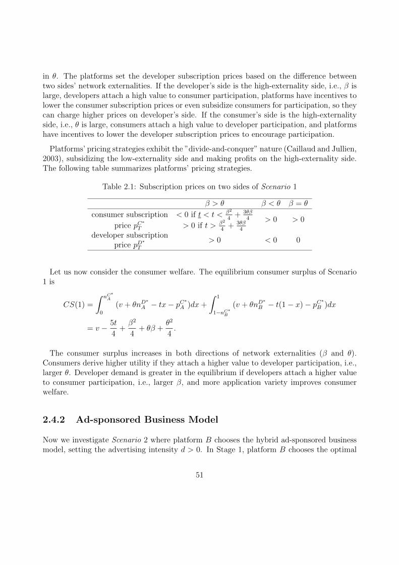
in θ. The platforms set the developer subscription prices based on the difference betweentwo sides’ network externalities. If the developer’s side is the high-externality side, i.e., β islarge, developers attach a high value to consumer participation, platforms have incentives tolower the consumer subscription prices or even subsidize consumers for participation, so theycan charge higher prices on developer’s side. If the consumer’s side is the high-externalityside, i.e., θ is large, consumers attach a high value to developer participation, and platformshave incentives to lower the developer subscription prices to encourage participation.

Platforms’ pricing strategies exhibit the ”divide-and-conquer” nature (Caillaud and Jullien,2003), subsidizing the low-externality side and making profits on the high-externality side.The following table summarizes platforms’ pricing strategies.

Table 2.1: Subscription prices on two sides of Scenario 1

β > θ β < θ β = θ

consumer subscription < 0 if t < t < β2

4+ 3θβ

4 > 0 > 0price pC

∗T > 0 if t > β2

4+ 3θβ

4

developer subscription> 0 < 0 0

price pD∗

T

Let us now consider the consumer welfare. The equilibrium consumer surplus of Scenario1 is

CS(1) =

∫ nC∗A

0

(v + θnD∗

A − tx− pC∗

A )dx+

∫ 1

1−nC∗B

(v + θnD∗

B − t(1− x)− pC∗B )dx

= v − 5t

4+β2

4+ θβ +

θ2

4.

The consumer surplus increases in both directions of network externalities (β and θ).Consumers derive higher utility if they attach a higher value to developer participation, i.e.,larger θ. Developer demand is greater in the equilibrium if developers attach a higher valueto consumer participation, i.e., larger β, and more application variety improves consumerwelfare.

2.4.2 Ad-sponsored Business Model

Now we investigate Scenario 2 where platform B chooses the hybrid ad-sponsored businessmodel, setting the advertising intensity d > 0. In Stage 1, platform B chooses the optimal

51

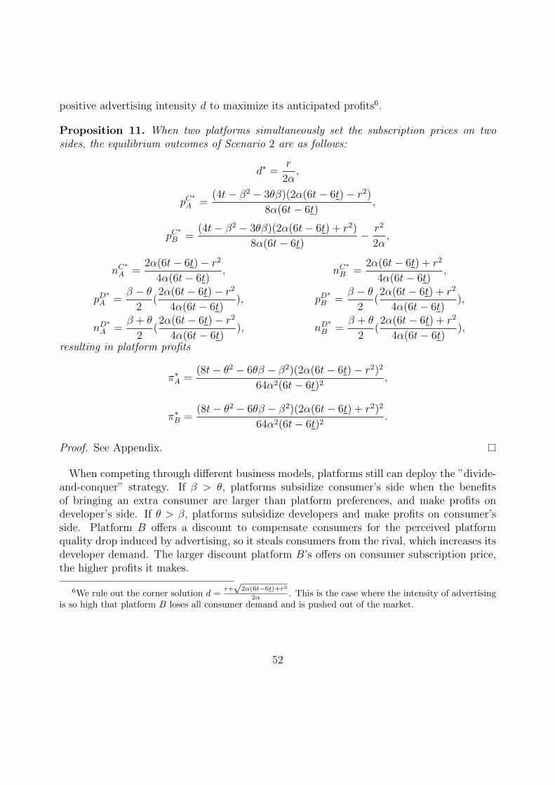
positive advertising intensity d to maximize its anticipated profits6.

Proposition 11. When two platforms simultaneously set the subscription prices on twosides, the equilibrium outcomes of Scenario 2 are as follows:

d∗ =r

2α,

pC∗

A =(4t− β2 − 3θβ)(2α(6t− 6t)− r2)

8α(6t− 6t),

pC∗

B =(4t− β2 − 3θβ)(2α(6t− 6t) + r2)

8α(6t− 6t)− r2

2α,

nC∗

A =2α(6t− 6t)− r2

4α(6t− 6t), nC

∗

B =2α(6t− 6t) + r2

4α(6t− 6t),

pD∗

A =β − θ

2(2α(6t− 6t)− r2

4α(6t− 6t)), pD

∗

B =β − θ

2(2α(6t− 6t) + r2

4α(6t− 6t)),

nD∗

A =β + θ

2(2α(6t− 6t)− r2

4α(6t− 6t)), nD

∗

B =β + θ

2(2α(6t− 6t) + r2

4α(6t− 6t)),


π∗A =(8t− θ2 − 6θβ − β2)(2α(6t− 6t)− r2)2

64α2(6t− 6t)2,

π∗B =(8t− θ2 − 6θβ − β2)(2α(6t− 6t) + r2)2

64α2(6t− 6t)2.


When competing through different business models, platforms still can deploy the ”divide-and-conquer” strategy. If β > θ, platforms subsidize consumer’s side when the benefitsof bringing an extra consumer are larger than platform preferences, and make profits ondeveloper’s side. If θ > β, platforms subsidize developers and make profits on consumer’sside. Platform B offers a discount to compensate consumers for the perceived platformquality drop induced by advertising, so it steals consumers from the rival, which increases itsdeveloper demand. The larger discount platform B’s offers on consumer subscription price,the higher profits it makes.

6We rule out the corner solution d =r+√

2α(6t−6t)+r2

2α . This is the case where the intensity of advertisingis so high that platform B loses all consumer demand and is pushed out of the market.

52

Table 2.2: Changes in equilibrium outcomes due to advertising (Scenario 2−Scenario 1)

β > θ β < θ β = θ

∆pC∗

A

> 0 if t < t < β2

4+ 3θβ

4 < 0 < 0< 0 if t > β2

4+ 3θβ

4

∆pC∗

B < 0> 0 if t < t < θ2

5+ 13θβ

20+ 3β2

20 < 0< 0 if t > θ2

5+ 13θβ

20+ 3β2

20

∆nC∗

A < 0 < 0 < 0∆nC

∗B > 0 > 0 > 0

∆pD∗

A < 0 > 0 0∆pD

∗B > 0 < 0 0

∆nD∗

A < 0 < 0 < 0∆nD

∗B > 0 > 0 > 0

∆π∗A < 0 < 0 < 0∆π∗B > 0 > 0 > 0

If the developer’s side is the high-externality side (β > θ), platform B lowers its consumersubscription price to compensate consumers for the disutility caused by advertising. PlatformA’s reaction on consumer’s side depends on whether the platforms are subsidizing consumersor not. If both platforms charge positive consumer subscription prices, platform A wouldfollow platform B’s price movement, lowering its consumer subscription prices as consumerprices are strategic complements (t > 3θβ

4+ β2

4); if both platforms subsidize consumers,

platform A would move against platform B’s pricing strategy, cutting its subsidy as consumerprices are strategic substitutes (t < t < 3θβ

4+ β2

4) (Besanko et al., 2000). Platform B expands

it consumers demand, so it can charge a higher developer subscription price and gains moredeveloper demand; while platform A has to lower its developer subscription price because itis now less valuable to developers, still loses some developer demand.

If the consumer’s side is the high-externality side (β < θ), consumers attach a high valueto developer participation. Platform B lowers its developer subscription price to expanddeveloper demand. Therefore, platform B becomes more valuable to consumers even in thepresence of adverts. When the network externalities are strong compared to platform pref-erences (t < t < θ2

5+ 13θβ

20+ 3β2

20), this is the case where a small extra developer demand can

lead to a large extra consumer demand, platform B can even increases its consumer sub-scription prices. When the network externalities are weak compared to platform preferences,platform B lowers its consumer subscription price to compensate for the disutility causedby advertising. Given a smaller consumer demand, platform A is better off to reduce itssubsidy on developer’s side.

If β = θ, platforms set the developer subscription price at the marginal cost, both platforms

53

charge lower the consumer subscription prices to compete for consumers. This is becauseboth platforms’ revenue rely on their consumer demands. Platform A only collects revenuefrom consumers subscription while platform B collects revenue from consumer subscriptionand its advertising revenue (which also depends on its consumer demand). Platform Bcan over-compensate consumers for disutility caused by advertising to expand its consumerdemand, hence, developer demand.

From a welfare standpoint, consumers are affected by platform B’s adverts through differ-ent channels. Firstly, consumers on platform B suffer utility loss because they view adverts asa nuisance. Secondly. both platforms adjust the consumer subscription prices, which affectsall consumers. Thirdly. consumers are affected by the changes in developer demands.

Proposition 12. When consumers have increasing marginal disutility towards advertising,consumers are better off when platform B adopts the hybrid ad-sponsored business model.


2.5 Extension: Sequential Price Setting

In this section, we are interested in a game where both platforms set the developer sub-scription prices before the consumer subscription prices. Thus, we propose the followingfour-stage game: In Stage 1, platform B chooses its advertising intensity. In Stage 2a, twoplatforms simultaneously set the developer subscription prices. In Stage 2b, two platformssimultaneously set the consumer subscription prices. In Stage 3, developers make participa-tion decisions. In Stage 4, consumers make participation decisions7. All the decisions arepublicly observable.

Let t1 = θ2

9+ 7θβ

9+ β2

9. The following proposition characterizes the competition outcomes

of Stage 2 as functions of advertising intensity d.

Proposition 13. When two platforms set the developer subscription prices before the con-sumer subscription prices, given platform B chooses the advertising intensity d in Stage 1,the competition outcomes of Stage 2 can be written as functions of d:

pCA(d) =6t− 5θβ + β2

3(3t− 3t1 + αd2 − rd

6t− 6t1),

pCB(d) =6t− 5θβ + β2

3(3t− 3t1 − αd2 + rd

6t− 6t1)− rd,

7The equilibrium outcomes of this game are the same as those of a three-stage game where developersand consumers arrive simultaneously in Stage 3 as long as all consumers hold responsive expectations

54

nCA(d) =3t− 3t1 + αd2 − rd

6t− 6t1,

nCB(d) =3t− 3t1 − αd2 + rd

6t− 6t1,

pDA(d) =β − θ

3(3t− 3t1 + αd2 − rd

6t− 6t1),

pDB(d) =β − θ

3(3t− 3t1 − αd2 + rd

6t− 6t1),

nDA(d) =2β + θ

3(3t− 3t1 + αd2 − rd

6t− 6t1),

nDB(d) =2β + θ

3(3t− 3t1 − αd2 + rd

6t− 6t1),


πA(d) =(18t− θ2 − 16θβ − β2)(t− t1 + αd2 − rd)2

(4(9t− 9t1))2,

πB(d) =(18t− θ2 − 16θβ − β2)(6t− 6t1 − αd2 + rd)2

(4(9t− 9t1))2.


We also identify 2 scenarios depending on platform B’s choice of advertising intensitywhen two platforms set the developer subscription prices before the consumer subscriptionprices:

Scenario 1’. Platform B sets the advertising intensity to be 0 in Stage 1.

Scenario 2’. Platform B sets the advertising intensity to be d∗ in Stage 1, which maximizesits anticipated equilibrium profits.

2.5.1 Subscription-based Business Model

We first derive the subgame equilibrium where platform B sets advertising intensity d = 0.The following proposition characterizes the equilibrium outcomes when platform B sets d = 0in Stage 1.

55

Proposition 14. When two platforms set the developer subscription prices before the con-sumer subscription prices, the equilibrium outcomes of Scenario 1′ are as follows:

pC∗

T = t− β2

6− 5θβ

6, nC

∗

T =1

2,

pD∗

T =β

6− θ

6, nD

∗

T =β

3+θ

6,

π∗T =t

2− θ2

36− 4θβ

9− β2

36,

where T = A,B.


In this scenario, the equilibrium consumer subscription price is also the standard Hotellingprice with zero marginal cost, which is t, adjusted downwards by the benefits of attractingan extra consumer. However, the benefits of attracting an extra consumer are different fromthose in Scenario 1. The platform attracts β extra developers when it has an extra consumer.Each extra developer pays a subscription price β

6− θ

6to the platform, also attracts θ extra

consumers. Platform subsidize consumers if the benefits of attracting one extra consumerare large compared to platform preferences.

Again, platforms set the developer subscription prices based on the difference between twodirections of network externalities. If two sides have symmetric network externalities (β = θ),platforms set the developer subscription prices at the marginal cost. If the developer’s sideis the high-externality side, platforms charge positive prices on this side; if the developer’sside is the low-externality side, platforms subsidize developers for participation.

Similarly, platforms deploy the ”divide-and-conquer” strategy to overcome the coordina-tion problem. The following table summarizes the platforms’ pricing strategies in Scenario1′.

Table 2.3: Subscription prices on two sides of Scenario 1′

β > θ β < θ β = θ

consumer subscription < 0 if t < t < β2

6+ 5θβ

6 > 0 > 0price pC

∗T > 0 if t > β2

6+ 5θβ

6

developer subscription> 0 < 0 0

price pD∗

T

We compare the equilibrium outcomes of Scenario 1′withthoseofScenario 1. The changesin equilibrium outcomes are summarized in the following table:

56

Table 2.4: Changes in equilibrium outcomes due to the order of price setting (Scenario1′−Scenario 1)

β > θ β < θ β = θ∆pC

∗T > 0 < 0 0

∆pD∗

T < 0 > 0 0∆nD

∗T > 0 < 0 0

∆π∗T > 0 > 0 0∆CS < 0 < 0 0

If two sides have symmetric network externalities (β = θ), the platforms fixate the devel-oper subscription prices at marginal cost, 0. Given that symmetric platforms compete formarket share on the fixed-sized consumer’s side, setting the developer subscription pricesbefore the consumer subscription prices results in the same equilibrium outcomes as settingthe subscription prices on both side simultaneously.

If two sides have asymmetric network externalities (β 6= θ) and competing platforms couldcoordinate the order of price setting, they could set the subscription prices on developer’sside before consumer’s side to increase platform profits. Price competition is intensified onthe high-externality side and is softened on the low-externality side. The intuition behindthis is as follows: when setting the prices on two sides simultaneously, the network exter-nalities are fully internalized; but setting the subscription prices on developer’s side beforeconsumer’s side dampens the two-sidedness, the network externalities are partially internal-ized, so platforms would compete more aggressively for users on the more profitable side (thehigh-externality side), and the low-externality side becomes less valuable.

2.5.2 Ad-sponsored Business Model

Now we investigate the subgame where platform B chooses the hybrid ad-sponsored businessmodel, i.e., d > 0. In Stage 1, platform B chooses the optimal positive advertising intensityd to maximize its anticipated profits.

Proposition 15. When two platforms set the developer subscription prices before the con-sumer subscription prices, the equilibrium outcomes of Scenario 2′ are as follows:

d∗ =r

2α,

pC∗

A =(6t− 5θβ − β2)(4α(3t− 3t1)− r2)

24α(3t− 3t1),

57

pC∗

B =(6t− 5θβ − β2)(4α(3t− 3t1) + r2)

24α(3t− 3t1)− r2

2α,

nC∗

A =4α(3t− 3t1)− r2

8α(3t− 3t1), nC

∗

B =4α(3t− 3t1) + r2

8α(3t− 3t1),

pD∗

A =β − θ

3(4α(3t− 3t1)− r2

8α(3t− 3t1)), pD

∗

B =β − θ

3(4α(3t− 3t1) + r2

8α(3t− 3t1)),

nD∗

A =θ + 2β

3(4α(3t− 3t1)− r2

8α(3t− 3t1)), nD

∗

B =θ + 2β

3(4α(3t− 3t1) + r2

8α(3t− 3t1)),


π∗A =(18t− θ2 − 16θβ − β2)(4α(3t− 3t1)− r2)2

576α2(3t− 3t1)2,

π∗B =(18t− θ2 − 16θβ − β2)(4α(3t− 3t1) + r2)2

576α2(3t− 3t1)2.


The next table presents the changes in prices and demands between Scenario 2′ andScenario 2 due to the change on the order of price setting.

Table 2.5: Changes in equilibrium outcomes due to the order of price setting (Scenario2′−Scenario 2)

β > θ β < θ β = θ∆pC

∗A 0

∆pC∗

B > 0 < 0 0∆nC

∗A > 0 0

∆nC∗

B < 0 0∆pD

∗A 0

∆pD∗

B < 0 > 0 0∆nD

∗A 0

∆nD∗

B < 0 0

The order of price setting does not change the equilibrium advertising intensity, but itdoes have an impact on consumer demand. The ad-sponsored business model is less effectivein expanding consumer demand when platforms set the subscription prices on developer’sside before consumer’s side. As explained before, this is because when platforms set pricesimultaneously on both sides, the externalities are fully internalized, which better coordinatesthe demands from both sides.

58

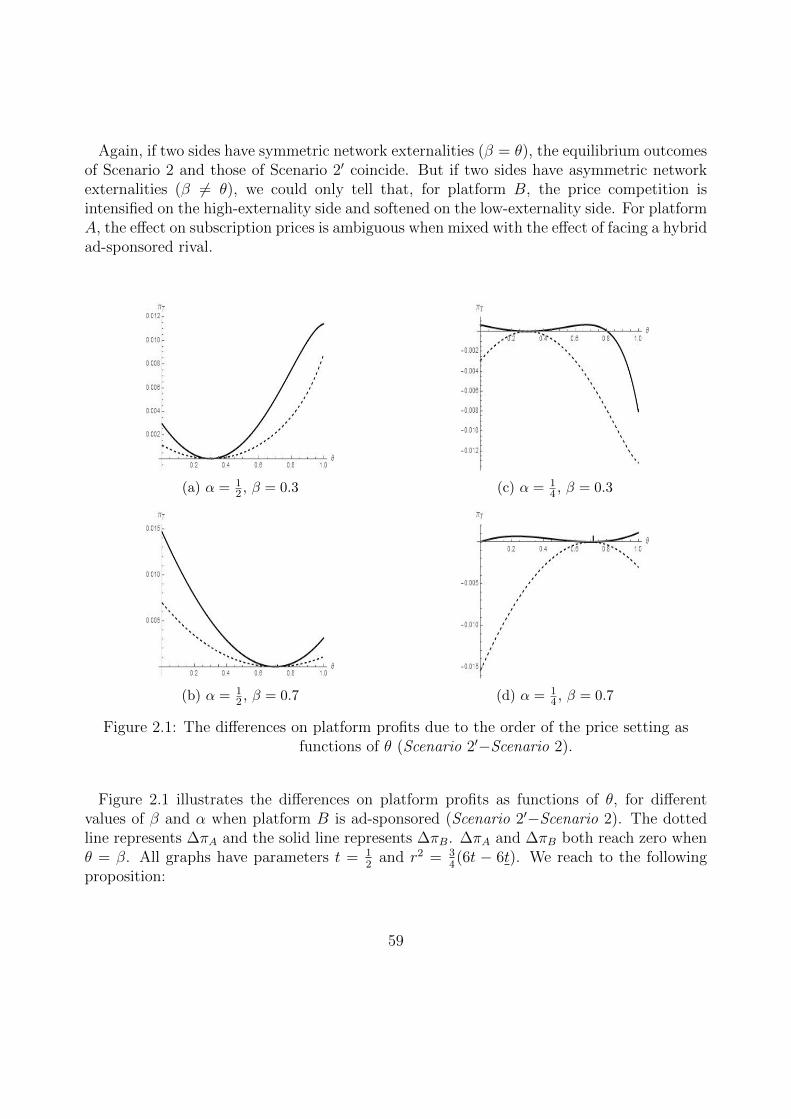
Again, if two sides have symmetric network externalities (β = θ), the equilibrium outcomesof Scenario 2 and those of Scenario 2′ coincide. But if two sides have asymmetric networkexternalities (β 6= θ), we could only tell that, for platform B, the price competition isintensified on the high-externality side and softened on the low-externality side. For platformA, the effect on subscription prices is ambiguous when mixed with the effect of facing a hybridad-sponsored rival.

(a) α = 12 , β = 0.3

(b) α = 12 , β = 0.7

(c) α = 14 , β = 0.3

(d) α = 14 , β = 0.7

Figure 2.1: The differences on platform profits due to the order of the price setting asfunctions of θ (Scenario 2′−Scenario 2).

Figure 2.1 illustrates the differences on platform profits as functions of θ, for differentvalues of β and α when platform B is ad-sponsored (Scenario 2′−Scenario 2). The dottedline represents ∆πA and the solid line represents ∆πB. ∆πA and ∆πB both reach zero whenθ = β. All graphs have parameters t = 1

2and r2 = 3

4(6t − 6t). We reach to the following

proposition:

59

Proposition 16. In the presence of symmetric network externalities (β = θ), if the con-sumer’s market size is fixed, platforms are indifferent between setting the developer subscrip-tion prices before the consumer subscription prices and setting the subscription prices on bothside simultaneously, regardless of platform B’s business model.


From the perspective of consumer welfare, under the hybrid ad-sponsored business model,the majority of consumers (consumers on platform B) are better off because of a lowersubscription price (which over-compensates the disutility caused by advertising) and moreapplication variety, while the minority of consumers (consumers on platform A) are worseoff, and the unequal split of consumer demand increase the aggregate transportation cost.Similarly, setting the subscription prices on developer’s side before consumer’s side createsboth positive and negative effects on consumer welfare. In general, the intensified pricecompetition on the high-externality side benefits consumers either by offering more appli-cation variety (if developer’s side is the high-externality side) or offering lower consumersubscription prices (if consumer’s side is the high-externality side); while the softened pricecompetition on the low-externality side harms consumers either by reducing application va-riety (if developer’s side is the low-externality side) or charging higher consumer subscriptionprices (if consumer’s side is the low-externality side). The following proposition characterizeshow consumer surplus is affected by platform B’s choice of business models and the order ofprice setting by both platforms.

Proposition 17. In a game where both platforms set the developer subscription prices be-fore the consumer subscription prices, consumers are better off when platform B adopts thehybrid ad-sponsored business model. They are worse off when platforms set the developerssubscription prices before the consumer subscription prices relative to the case where plat-forms set the subscription prices on both sides simultaneously, regardless of platform B’sbusiness model.


2.6 Conclusion

This paper analyzes the platform’s strategic choices of business models between the puresubscription-based and the hybrid ad-sponsored business models when competing with asubscription-based rival. The fact that high technology-based platforms usually have oneside of users (developers) arriving before the other side users (consumers) is also feature

60

in this paper. We show that, in the setting of single-homing consumers and multi-homingdevelopers, when consumers have increasing marginal disutility towards advertising, it isprofitable to adopt the hybrid ad-sponsored business model independent of the degree ofnetwork externalities, and it is detrimental to the rival. This result holds no matter whetherthe platforms set the subscription prices on both sides simultaneously or set the developersubscription prices before the consumer subscription prices.

We shed light on platforms’ incentives to set the subscription prices on each side in asequential fashion rather than simultaneously. We show that, when competing through thesubscription-based business model, setting the developer subscription prices before consumerprices intensifies price competition on the high-externality side and softens competition onthe low-externality side. Platforms exploit more profits at the expense of consumers. Whentwo platforms compete through different business models, price competition is also intensifiedon the high-externality side and softened on the low-externality side for platform B, but forplatform A, the effect on subscription prices is ambiguous when mixed with the effect offacing a hybrid ad-sponsored rival.

From a welfare standpoint, it improves consumer welfare when platform B adopts the hy-brid ad-sponsored business model no matter whether platforms set the subscription prices onboth sides simultaneously or set the developer subscription prices before the consumer sub-scription prices. We also show that consumers are better of if platforms set the subscriptionprices on both sides simultaneously.

We notice that a dual business model where the platform offers consumers both the puresubscription-based service and the pure ad-sponsored service is often used in reality. Forinstance, on most Chinese online video platforms, the viewers can either pay subscriptionfees to watch the video contents or watch some adverts in exchange for watching the videocontents for free. A pressing step for future research is to allow the platform to have thechoice of adopting the dual business model. When competing with a pure subscription-basedrival, the dual business model seems to have a competitive advantage. However, the analysisof the competition between the hybrid ad-sponsored model and the dual business modelcould provide new insights into platform’s business strategies. We leave this analysis forfuture research.

61

Appendix

Proof of Proposition 9In Stage 4, consumers make their participation decisions given pCT set in Stage 2 and nDTrealized in Stage 3, as well as the advertising intensity d chosen by platform B in Stage 1.The consumer demands are

nCA =1


2t+θnDA − θnDB

2t,

and

nCB =1


2t+θnDB − θnDA

2t.

In Stage 3, The developer demand is

nDT = βnCe

T − pDT ,

where nCe

T = nCT for any given price pair (pCT , pDT ), T = A,B. The implied consumer demands

for each platform are:

nCA =1



and

nCB =1



.

In Stage 2, given platform B’s advertising intensity d, the platforms choose the subscriptionprices on two sides simultaneously. Platform A’s profit maximization problem is

maxpCA,p

DA

πA = pCAnCA + pDAn

DA ,

and platform B’s profit maximization problem is

maxpCB ,p

DB

πB = pCBnCB + pDBn

DB + rdnCB.

Taking the first order conditions in pCT and pDT , given d, we obtain the following first ordercondition equations:

pCA(d, pCB, pDA , p

DB) =

t− θβ2

+1

2pCB −

θ + β

2pDA +

θ

2pDB +

αd2

2,

pDA(d, pCA, pCB, p

DB) =

β(t− θβ)− (θ + β)pCA + βpCB + θβpDB4t− 2θβ

+αd2β

4t− 2θβ,

62

pCB(d, pCA, pDA , p

DB) =

t− θβ2

+1

2pCA −

θ + β

2pDB +

θ

2pDA −

rd+ αd2

2and

pDB(d, pCA, pCB, p

DB) =

β(t− θβ)− (θ + β)pCB + βpCA + θβpDA4t− 2θβ

− αd2β + θrd

4t− 2θβ.

Solving the system of the first order equations, we obtain prices and demands as functionsof d:

pCA(d) =(4t− 3θβ − β2)(6t− 6t− 2rd+ 2αd2)

4(6t− 6t),

pCB(d) =(4t− 3θβ − β2)(6t− 6t+ 2rd− 2αd2)

4(6t− 6t)− rd,

nCA(d) =1

2− rd− αd2

6t− 6t, nCB(d) =

1

2+rd− αd2

6t− 6t,

pDA(d) =β − θ

2(1

2− rd− αd2

6t− 6t), pDB(d) =

β − θ2

(1

2+rd− αd2

6t− 6t),

and nDA(d) =β + θ

2(1

2− rd− αd2

6t− 6t), nDB(d) =

β + θ

2(1

2+rd− αd2

6t− 6t),


πA(d) =(8t− θ2 − 6θβ − β2)(6t− 6t− 2rd+ 2αd2)2

16(6t− 6t)2

and

πB(d) =(8t− θ2 − 6θβ − β2)(6t− 6t+ 2rd− 2αd2)2

16(6t− 6t)2.

Proof of Proposition 11In Proposition 1, we have obtain the prices and demands as functions of advertising intensityd:

pCA(d) =(4t− 3θβ − β2)(6t− 6t− 2rd+ 2αd2)

4(6t− 6t),

pCB(d) =(4t− 3θβ − β2)(6t− 6t+ 2rd− 2αd2)

4(6t− 6t)− rd,

nCA(d) =1

2− rd− αd2

6t− 6t, nCB(d) =

1

2+rd− αd2

6t− 6t,

pDA(d) =β − θ

2(1

2− rd− αd2

6t− 6t), pDB(d) =

β − θ2

(1

2+rd− αd2

6t− 6t),

63

and nDA(d) =β + θ

2(1

2− rd− αd2

6t− 6t), nDB(d) =

β + θ

2(1

2+rd− αd2

6t− 6t),


πA(d) =(8t− θ2 − 6θβ − β2)(6t− 6t− 2rd+ 2αd2)2

16(6t− 6t)2

and

πB(d) =(8t− θ2 − 6θβ − β2)(6t− 6t+ 2rd− 2αd2)2

16(6t− 6t)2.

In Satge 1, platform B chooses the advertising intensity d to maximize its anticipated profits,we obtain the market-sharing equilibrium advertising intensity d∗ = r

2α. Therefore the

equilibrium prices and allocations are as follows:

pC∗

A =(4t− β2 − 3θβ)(2α(6t− 6t)− r2)

8α(6t− 6t),

pC∗

B =(4t− β2 − 3θβ)(2α(6t− 6t) + r2)

8α(6t− 6t)− r2

2α,

nC∗

A =2α(6t− 6t)− r2

4α(6t− 6t), nC

∗

B =2α(6t− 6t) + r2

4α(6t− 6t),

pD∗

A =β − θ

2(2α(6t− 6t)− r2

4α(6t− 6t)), pD

∗

B =β − θ

2(2α(6t− 6t) + r2

4α(6t− 6t)),

nD∗

A =β + θ

2(2α(6t− 6t)− r2

4α(6t− 6t)), nD

∗

B =β + θ

2(2α(6t− 6t) + r2

4α(6t− 6t)),


π∗A =(8t− θ2 − 6θβ − β2)(2α(6t− 6t)− r2)2

64α2(6t− 6t)2,

π∗B =(8t− θ2 − 6θβ − β2)(2α(6t− 6t) + r2)2

64α2(6t− 6t)2.

Proof of Proposition 12In Scenario 2, the equilibrium consumer surplus is

CS(2) = v − 5

4t+

β2

4+ θβ +

θ2

4+r2(r2t+ 2α(6t− 6t)2)

16α2(6t− 6t)2,

Therefore, the difference in equilibrium consumer surplus due to platform B’s choice ofbusiness models is

∆CS = CS(2)− CS(1) =r2(r2t+ 2α(6t− 6t)2)

16α2(6t− 6t)2> 0.

64

Proof of Proposition 13In Stage 4, given that the advertising intensity and all subscription prices are set, developershave already made their participation decisions, the consumer demands are:

nCA =1


2t+θnDA − θnDB

2t,

nCB =1


2t+θnDB − θnDA

2t,

where the developer demandsnDA = βnC

e

A − pDAand

nDB = βnCe

B − pDBare realized in Stage 3. Developers have the information about the advertising intensity dand the subscription prices on both sides, their expectations about consumer demand matchthe realized consumer demand. Hence, the implied consumer demands are:

nCA =1



,

and

nCB =1



.

In Stage 2b, given the advertising intensity and the developer subscription prices are alreadyset, the platforms choose the consumer subscription prices to maximize profits. PlatformA’s profit maximization problem is

maxpCA

πA = pCAnCA + pDA(βnCA − pDA),

and platform B’s profit maximization problem is

maxpCB

πB = pCBnCB + pDB(βnCB − pDB) + rdnCB.

Taking the first-order condition in the consumer subscription prices, we obtain the followingfirst order condition equations:

pCA(d, pCB, pDA , p

DB) =

t− θβ2

+pCB2− θ + β

2pDA +

θ

2pDB +

αd2

2

and

pCB(d, pCA, pDA , p

DB) =

t− θβ2

+pCB2− θ + β

2pDA +

θ

2pDB −

αd2

2− rd

2.

65

Therefore, we obtain the consumer subscription prices and two sided demands as functionsof the advertising intensity and the developer subscription prices:

pCA(d, pDA , pDB) = t− θβ − θ + 2β

3pDA +

θ − β3

pDB +αd2 − rd

3,

pCB(d, pDA , pDB) = t− θβ − θ + 2β

3pDB +

θ − β3

pDA −αd2 + 2rd

3,

nCA(d, pDA , pDB) =

1

2− θ − β

6t− 6θβpDA +

θ − β6t− 6θβ

pDB +αd2 − rd6t− 6θβ

,

nCB(d, pDA , pDB) =

1

2− θ − β

6t− 6θβpDB +


pDA −αd2 − rd6t− 6θβ

,

nDA(d, pDA , pDB) = β(

1

2− θ − β

6t− 6θβpDA +


pDB +αd2 − rd6t− 6θβ

)− pDA ,

and

nDB(d, pDA , pDB) = β(

1

2− θ − β

6t− 6θβpDB +


pDA −αd2 − rd6t− 6θβ

)− pDB .

In Stage 2a, platforms set the developer subscription prices to maximize its profits. Takingthe first-order condition in the developer subscription prices, we obtain the system of bestresponse functions:

pDA(d, pDB) =3(t− θβ)(β − θ)

18t− θ2 − 16θβ − β2+

d(αd− r)(β − θ)18t− θ2 − 16θβ − β2

− (β − θ)2pDB18t− θ2 − 16θβ − β2

,

and

pDB(d, pDA) =3(t− θβ)(β − θ)

18t− θ2 − 16θβ − β2− d(αd− r)(β − θ)

18t− θ2 − 16θβ − β2− (β − θ)2pDA

18t− θ2 − 16θβ − β2.

Let t1 = θ2

9− 7θβ

9− β2

9. It’s straightforward to obtain the prices and demands as functions

of advertising intensity d:


3(3t− 3t1 + αd2 − rd

6t− 6t1),


3(3t− 3t1 − αd2 + rd

6t− 6t1)− rd,

nCA(d) =3t− 3t1 + αd2 − rd

6t− 6t1,

66

nCB(d) =3t− 3t1 − αd2 + rd

6t− 6t1,

pDA(d) =β − θ

3(3t− 3t1 + αd2 − rd

6t− 6t1),

pDB(d) =β − θ

3(3t− 3t1 − αd2 + rd

6t− 6t1),

nDA(d) =2β + θ

3(3t− 3t1 + αd2 − rd

6t− 6t1),

nDB(d) =2β + θ

3(3t− 3t1 − αd2 + rd

6t− 6t1),


πA(d) =(18t− θ2 − 16θβ − β2)(t− t1 + αd2 − rd)2

(4(9t− 9t1))2,

πB(d) =(18t− θ2 − 16θβ − β2)(6t− 6t1 − αd2 + rd)2

(4(9t− 9t1))2.

Proof of Proposition 15In Proposition 5, we present the prices and demands as functions of d:


3(3t− 3t1 + αd2 − rd

6t− 6t1),


3(3t− 3t1 − αd2 + rd

6t− 6t1)− rd,

nCA(d) =3t− 3t1 + αd2 − rd

6t− 6t1,

nCB(d) =3t− 3t1 − αd2 + rd

6t− 6t1,

pDA(d) =β − θ

3(3t− 3t1 + αd2 − rd

6t− 6t1),

pDB(d) =β − θ

3(3t− 3t1 − αd2 + rd

6t− 6t1),

nDA(d) =2β + θ

3(3t− 3t1 + αd2 − rd

6t− 6t1),

67

nDB(d) =2β + θ

3(3t− 3t1 − αd2 + rd

6t− 6t1),


πA(d) =(18t− θ2 − 16θβ − β2)(t− t1 + αd2 − rd)2

(4(9t− 9t1))2,

πB(d) =(18t− θ2 − 16θβ − β2)(6t− 6t1 − αd2 + rd)2

(4(9t− 9t1))2.

In Stage 1, platform B chooses the optimal advertising intensity d to maximize its antic-ipated profits. The market-sharing equilibrium advertising intensity is d∗ = r

2α, and the

equilibrium prices and allocations are as follows:

pC∗

A =(6t− 5θβ − β2)(4α(3t− 3t1)− r2)

24α(3t− 3t1),

pC∗

B =(6t− 5θβ − β2)(4α(3t− 3t1) + r2)

24α(3t− 3t1)− r2

2α,

nC∗

A =4α(3t− 3t1)− r2

8α(3t− 3t1), nC

∗

B =4α(3t− 3t1) + r2

8α(3t− 3t1),

pD∗

A =β − θ

3(4α(3t− 3t1)− r2

8α(3t− 3t1)), pD

∗

B =β − θ

3(4α(3t− 3t1) + r2

8α(3t− 3t1)),

nD∗

A =θ + 2β

3(4α(3t− 3t1)− r2

8α(3t− 3t1)), nD

∗

B =θ + 2β

3(4α(3t− 3t1) + r2

8α(3t− 3t1)),


π∗A =(18t− θ2 − 16θβ − β2)(4α(3t− 3t1)− r2)2

576α2(3t− 3t1)2,

π∗B =(18t− θ2 − 16θβ − β2)(4α(3t− 3t1) + r2)2

576α2(3t− 3t1)2.

Proof of Proposition 16When platform B is subscription-based, the differences on equilibrium outcomes due to thechange of the order of price setting are as follows (Scenario 1′-Scenario 1):

∆pC∗

T =β(β − θ)

12, ∆nC

∗

T = 0,

∆pD∗

T =(θ − β)

12, ∆nD

∗

T =β − θ

12,

∆π∗T =5(β − θ)2

144,

68

where T = A,B.

In the presence of symmetric network externalities (β = θ), the difference in equilibriumoutcomes become

∆pC∗

T = 0, ∆nC∗

T = 0,

∆pD∗

T = 0, ∆nD∗

T = 0,

∆π∗T = 0,

where T = A,B.

When platform B is ad-sponsored, the differences on equilibrium prices and allocationsdue to the change of the order of price setting are as follows (Scenario 2′-Scenario 2):

∆pC∗

A =(θ − β)(−3(2θ + β)(t− θβ)r2 + β(6t− 6t)(9t− 9t1))

12(6t− 6t)(9t− 9t1),

∆pC∗

B =(β − θ)(3(2θ + β)(t− θβ)r2 + β(6t− 6t)(9t− 9t1))

12(6t− 6t)(9t− 9t1),

∆nC∗

A =r2(β − θ)2

4(6t− 6t)(9t− 9t1), ∆nC

∗

B = − r2(β − θ)2

4(6t− 6t)(9t− 9t1),

∆pD∗

A =(θ − β)(−9(t− θβ)r2 + (6t− 6t)(9t− 9t1))

12(6t− 6t)(9t− 9t1),

∆pD∗

B =(θ − β)(9(t− θβ)r2 + (6t− 6t)(9t− 9t1))

12(6t− 6t)(9t− 9t1),

∆nD∗

A =(β − θ)((−9t+ 6θβ + 3β2)r2 + (6t− 6t)(9t− 9t1))

12(6t− 6t)(9t− 9t1),

∆nD∗

B =(β − θ)((9t− 6θβ − 3β2)r2 + (6t− 6t)(9t− 9t1))

12(6t− 6t)(9t− 9t1).

In the presence of symmetric network externalities (β = θ), the difference in equilibriumoutcomes become

∆pC∗

A = 0, ∆pC∗

B = 0,

∆nC∗

A = 0, ∆nC∗

B = 0,

∆pD∗

A = 0, ∆pD∗

B = 0,

∆nD∗

A = 0, ∆nD∗

B = 0,resulting in the differences on platform profits

∆π∗A = 0, ∆π∗B = 0.

69

Proof of Proposition 17In a game where platforms set the developer subscription prices before the consumer sub-scription prices:When platform B is subscription-based (Scenario 1′), the equilibrium consumer surplusis

CS(1′) = v − 5

4t+

β2

6+

7

6θβ +

θ2

6.

When platform B is ad-sponsored (Scenario 2′), the equilibrium consumer surplus is

CS(2′) = v − 5

4t+

β2

6+

7

6θβ +

θ2

6+r2(9r2t+ 8α(9t− 9t1)2)

64α2(9t− 9t1)2.

The change in consumer surplus due to platform B’s choice of business model is

∆CS = CS(2′)− CS(1′) =r2(9r2t+ 8α(9t− 9t1)2)

64α2(9t− 9t1)2> 0.

Therefore, consumers are better off in the presence of adverts when platforms set the devel-oper subscription prices before the consumer subscription prices.

Recall that in the game where platforms set the subscription prices on both sides simulta-neously, when platform B is subscription-based, the equilibrium consumer surplus is

CS(1) = v − 5

4t+

β2

4+ θβ +

θ2

4.

Therefore, the difference in equilibrium consumer surplus due to the order of price settingis

∆CS = CS(1′)− CS(1) = −(θ − β)2

12< 0.

Therefore, gievn platform B is subscription-based, consumers are worse off when platformsset the developer subscription prices before the consumer subscription prices.

The equilibrium consumer surplus of Scenario 2′ is

CS(2′) = v − 5

4t+

β2

6+

7

6θβ +

θ2

6+r2(9r2t+ 8α(9t− 9t1)2)

64α2(9t− 9t1)2,

Recall that the equilibrium consumer surplus of Scenario 2 is

CS(2) = v − 5

4t+

β2

4+ θβ +

θ2

4+r2(r2t+ 2α(6t− 6t)2)

16α2(6t− 6t)2.

70

Therefore, the difference in equilibrium consumer surplus is

∆CS = CS(2′)− CS(2) = −(θ − β)2

12+r4t(θ − β)2(5θ2 + 26θβ + 5β2 − 36t)

64α2(9t− 9t1)2(6t− 6t)2.

5θ2 + 26θβ + 5β2− 36t < 0 for all t > t, so ∆CS = CS(2′)−CS(2) < 0. So, gievn platformB is ad-sponsored, consumers are worse off when platforms set the developer subscriptionprices before the consumer subscription prices.We conclude that consumers are worse off when platforms set the developer subscriptionprices before the consumer subscription prices regardless of platform B’s choice of businessmodel.

71

Chapter 3

How venture capitalist compensationaffects investment decisionsjoint with Nuno Alvim

3.1 Introduction

A venture capital fund is typically formed under the limited partnership agreement. Theagreement rules the behavior of the investors and the venture capitalist (VC) in the rela-tionship over the entire life of the fund. Individual and institutional investors serve as thelimited partners (LPs), and the VC runs the fund as the general partner. The partnershipagreement explicitly specifies the terms of VC compensation, which consist of both visibleand invisible components. The visible components are management fee and carried interest(Da Rin et al., 2011), which have received full attention from both the industry insiders andacademic scholars1. The invisible component is the value-of-distribution rules that determinewhen the VC receives his carry (Litvak, 2009). A venture fund makes several investments atdifferent times throughout its life, and each investment has its exit date. The VC can eitherreceive his carry at the investment exit date or wait until the fund liquidates. A recent studysuggests that when the VC receives his carry becomes an important issue: early distributionof the carries reduces the costs of outside borrowing and creates correct incentives for theVC who control investment decisions (Litvak, 2009). Given the roles of capital provider anddecision maker are separated, the VC and the LPs potentially have a conflict of interestsand distort their valuation of the same projects: the VC only receives a share of profitsbut incurs costs of monitoring the projects. Identifying and analyzing these conflicts underdifferent types of the value-of-distribution rules is the main goal of this paper.

1See Gompers and Lerner (1996), Gompers and Lerner (1999), Metrick and Yasuda (2010).

72

This paper theoretically explores how the value-of-distribution rules affect the VC’s in-centives on the timing of investment and exit decisions, hence the duration, of investments.The value-of-distribution rules we look into are ”Escrow, all interest to fund” (the Escrowcontract), ”Return all capital contributions first” (the Return First contract) and ”Paybackwith no interest note” (the Payback contract) (Litvak, 2009). Under the Escrow contract,the VC’s share of profits goes to an escrow account when each investment is realized. TheVC only receives payments at the fund liquidation date and the interest of this accountgoes to the LPs, which generates an interest-free loan from the VC to the LPs. Under theReturn First contract, the VC receives no distributions until the invested capital has beenfully paid back to the LPs for each investment. After this threshold, the VC can receive hiscarry at each exit date. There should be no interest-free loan between the two parties oncethe invested capital is returned. Under the Payback contract, the VC receives his share ofthe revenues at the investment exit date and pays back the invested capital back to the LPswithout interest when the fund liquidates. This type of contract generates an interest-freeloan from the LPs to the VC.

We provide the first-best outcomes where the roles of capital provider and decision makerscoincide as a benchmark, then compare the investment decisions under different value-of-distribution rules with the first-best outcomes. The results we find are the following. If thereis only one project under consideration, the first-best exit date arrives when the marginalcost of staying in the investment equals to the marginal benefits of staying, and the investorwants to start the investment as early as possible. Under the Escrow contract, the first-bestinvestment duration can be attained give a certain level of the carried interest for the VC,but the VC would postpone the starting date of the investment because he wants to shortenthe period during which he practically lends an interest-free loan to the LPs. Under thePayback contract, there is practically an interest-free loan from the LPs to the VC, theVC would start the project early and exit from the project early to keep the loan periodlong. So, under the Payback contract, the optimal starting date can be attained but theduration of the project is always shorter than the optimal. Given a certain level of the carriedinterest, both the first-best investment duration and the starting date can be attained underthe Return First contract because there is no interest-free loan between the two parties. Ifthere are two investment projects under consideration, fixing the project that starts firstto be normal, the project that ends first incurs higher marginal monitoring cost becausethe investor has convex monitoring cost when there are two active projects. Therefore, theproject that ends first has a shorter first-best duration than that of the one project case, andthe project that ends second has the same first-best duration as that of the one project case.The investor wants to start both project as early as possible. Only the Escrow contract canrestore the first-best investment durations given a certain level of the carried interest for theVC, but cannot achieve the first-best starting dates. The first-best starting dates are possibleto be attained only under the Payback contract. Our results indicate that, regarding the

73

investment durations, using a certain level of carried interest can overcome the distortionsinduced by the interest-free loan, but not the distortion induced by the fact that the VCdoes not return the invested capital at the exit date.

To the best of our knowledge, this paper is the first attempt to analyze the impact of thevalue-of-distribution rules on investment decisions. The main contribution of the paper liesin highlighting the impact of the interest-free loan between the VC and the LPs generatedunder different types of distribution rules. The fact that the VC can only keep his share ofprofits instead of revenues makes monitoring costs relatively larger pushes for an early exitfrom investment projects. The interest-free loan from the LPs to the VC pushes for an earlyexit while the interest-free loan from the VC to the LPs has a contradicting effect. Withthese incentives, we study the efficiency of different distribution rules. We show that theReturn First contract can provide first-best outcomes when there is only one project. InLitvak (2009)’s sample, the Return First contract is the most popular one, used by almosthalf of the funds. However, when there are two projects under consideration, the Escrowcontract, which is the least-VC friendly contract, can restore the first-best durations givena certain level of the carried interest. In Litvak (2009)’s sample, the Escrow contract is theleast used one. We try to provide an answer to the question why Return First contractis popular than the others although it cannot provide first-best investment durations whenthere are two projects. Gompers and Lerner (1996) find empirical evidence suggest thatthe price of venture capital services shift if the demand for venture funds changes while thesupply of fund managers remains fixed in the short-run.

This paper is related to the literature on the conflict of interests between the VC andthe LPs in a venture capital fund. Compared with the extensive literature on the contractsbetween the VC and their portfolio enterprises, little light has been shed on the contractsbetween the VC and the LPs of venture funds. To the best of our knowledge, there areonly a few research papers studying the elements of venture capital limited partnershipagreement. Kandel et al. (2011) explore the cost of the limited life span of venture capitalfunds, featuring the VC’s informational advantage over the LPs and outsiders. They offerthe first-best outcome where no limited life span is imposed as the benchmark. They showthat the limited life span creates two types of ”myopia” on the VC’s investment decisionsand project choices relative to the first-best case: firstly, the VC may prefer to continue badprojects and sell them as unfinished good ones as long as the outsiders cannot distinguishthem, therefore, the first-best outcome is not likely to achieve; secondly, the VC does notmonitor good but delay-prone projects if he is not sufficiently compensated. Banal-Estanoland Ippolito (2012) focus on default penalties of the committed capital of private equityfunds. They argue that commitment by the LPs can reduce the cost of screening generalpartners by limiting ex-post renegotiation, and show that the degree of commitment bearimplications for the investment size of the fund and on the fee structure of the generalpartners.

74

This paper also relates to several studies on VC compensation, mostly empirical. The LPscannot get involved in the daily management of the funds. Therefore, the VC compensationis the most important contractual mechanism for aligning the incentives of the LPs andthe VC (Gompers and Lerner, 1999). Gompers and Lerner (1999) empirically examine VCcompensation with a dataset containing 419 partnerships dated from 1978 to 1992. In theirsample, They observe that the VC compensation is higher for older and larger funds; thepay of new VCs is less sensitive to performance because reputational concerns induce themto work hard Gompers and Lerner (1999) report that 81 percent of the funds in their sampleuse the classic 20 percent carry for the VC. Metrick and Yasuda (2010) study both venturecapital and leveraged buyout funds. They use a sample of 238 funds raised between 1993 and2006, 95 percent of which use the classic 20 percent carry. In both papers, only the visiblecomponents of VC compensation (management fee and carried interest) are considered, thevalue-of-distribution rules are ignored.

Our study is inspired by Litvak (2009), which is the first study that pays attention tothe value-of-distribution rules. Litvak (2009) suggests that the value-of-distribution rulesshould be the third element of VC compensation, along with the visible components (man-agement fee and carried interest). Through the interest-free loan generated by the value-of-distribution rules, the VC almost always captures a higher fraction of funds’ profits thanthe nominal carry percentage. Using a hand-collected dataset2, she shows that the timing ofdistribution matters because it is highly valuable to the VC: a shift from the most populardistribution rule to the second most popular rule can affect the VC compensation as muchor more than common variations in management fee or carried interest. Also, more complexmanagement fee provisions predict lower total compensation while common proxies for VCquality predict higher levels of the visible components of VC compensation (carried inter-est and management fee) but offers no prediction of the levels of invisible component (thevalue-of-capital distribution rules).

This paper proceeds as follows. Section 3.2 introduces the model. The first-best out-comes are presented in Section 3.3 as the benchmark cases. The impact of different typesdistribution rules is analyzed in Section 3.4. The last section concludes.

3.2 The Model

There are projects that each needs an investment F . The value of the project depends onthe duration of the investment d in two ways. Firstly: longer duration increases the valueof a normal project V (d) in a decreasing rate, i.e., V ′(d) > 0 and V ′′(d) < 0. Secondly: the

2Litvak (2009)’s sample consists of partnership agreements of 68 venture capital funds, raised by 28venture capital firms.

75

project may either remain normal or fail. The event of a failed project follows a Poissonprocess with intensity parameter λF . A failed project pays 0. We also consider that if aproject has shown to be a failure, the uncertainty is realized3. It means that a project canonly change state if it is normal. Therefore, the probability that a project fails at any givenmoment t is λF e

−λF t. The revenue of a normal project can either be sufficient to compensatethe invested capital, i.e. V (d) > F , or not, i.e., V (d) < F . If it cannot compensate theinvested capital, i.e. V (d) < F , the VC will terminate the project immediately. So, we onlyconsider the case V (d) > F .

The VC is risk neutral, cash poor and cares about his monetary returns. Time is continuousand is discounted at rate r. The VC has to monitor the project, due to his limited timeand energy, we consider that there is a convex cost of doing so: when there are two activeinvestment projects at the same time, the VC will need more personnel to monitor theseinvestments just to keep the monitoring intensity at the same level as that of one project.The monitoring costs incurred to the VC up to time t is

c(da, db, t) = δ

∫ t

a

(Φa(da, t) + Φb(db, t))2dτ,

0≤a≤b≤t,where Φi(di, t) = 1 if project i is active at time t and 0 otherwise. The subscripts a and bindicate the starting date of each project. The VC decides when to invest in the project andwhen to exit, hence its duration. We present all the expressions in future value evaluated atT , which is the fund liquidate date, it allows a nature comparison between different types ofthe value-of-distribution rules that the VC and the LPs sign.

We assume that the following conditions hold throughout this paper:Assumption A8. V ′(d)− λFV (d) > rV (d).

The marginal benefits of staying in an investment project are greater than the opportunitycosts of staying.Assumption A9. r(δ + V (dN)(r + λF )) > edN (r+λF )(r(F (r + λF ) + δ) + 2δ(r + λF )).

We assume that the investor’s marginal opportunity costs of investing are smaller than hismarginal costs of staying in the investment, so that we can ignore the question whether toinvest or not, and focus on the starting and exit decisions. This condition ensures that theinvestor invests4.

3Venture funds invest in portfolio enterprises that have a novel technology or business model in somehigh-technology industries, such as biotechnology, IT, software, etc; they offer high potential but high risk(Sahlman, 1990). Once the portfolio enterprises fail, venture funds usually just write them down or off. Theamazing story of how Steve Jobs brought Apple from near bankruptcy to billions is rather rare.

4The VC does not own any capital, he receives a share of profits only if he makes investments. So wefocus on the VC’s starting and exit decisions of investments

76

3.3 First-best outcomes

We derive the first-best outcomes where the roles of capital provider and investment de-cision maker coincide as a benchmark. The investment projects have the aforementionedcharacteristics.

3.3.1 One Project

We start with the case where there is only one investment project under consideration. Fornow, we assume this project starts at date 0, which is also the starting date of the venturefund. The investor must evaluate whether to exit from or remain in the investment at eachpoint in time. If the project fails, the investor will terminate the investment immediately.There will be no revenue, but further monitoring cost can be avoided by exiting. At date 0,the expected profits of having a project with duration d, as long as it remains normal, are

E(Π(dN)) = e−λF dN (er(T−dN )V (dN)−∫ dN

0

δer(T−τ)dτ)

+

∫ dN

0

λF e−λF t(−

∫ t

0

δer(T−τ)dτ)dt− erTF.(3.1)

The first part of the first two terms concerns the probability of being at each specific stateafter duration d and the second part (in brackets) concerns the future value of the payoff(net of monitoring costs) of each possible state, minus the invested capital of the project,evaluated at date T .

The investor solves the following profit maximization problem:

maxdN

E(Π(dN)).

The investor’s strategy is determined by a first order condition that depends on whetherthe optimal exit date of a normal project has passed or not.

∂E(Π(dN))

∂dN= e−λF dN+r(T−dN )(−λF − r)V (dN) + e−λF dN+r(T−dN )V ′(dN)

− e−λF dN (er(T−dN ) − (erT − er(T−dN ))λF )δ

− λF δ

r(erT−dNλF − er(T−dN )−dNλF ).

77

If the project remains normal, then the exit condition is

rV (d∗N) + δ = V ′(d∗N)− λFV (d∗N). (3.2)

On the left hand side we have the marginal costs of staying in the investment project,which consist of the interest opportunity costs and the increase in monitoring cost. On theright hand side lies the marginal benefits of staying, which include not only the growth of aregular project, but also the possibility that a project fails and all the revenue is lost.

We then ask when the investor wants to start the project if it does not necessarily startsat date 0. Assume the investor starts the investment at date a, which may or may not be 0.The investor’s expected profits are

E(Π(dN , a)) = e−λF dN (er(T−dN−a)V (dN)−∫ a+dN

a

δer(T−τ)dτ)

+

∫ dN

0

λF e−λF t(−

∫ a+t

a

δer(T−τ)dτ)dt− er(T−a)F.

The investor makes the starting decision by taking the first derivatives of the expectedprofits of starting date a. The derivative with respect to a is

∂E(Π(dN , a))

∂a= −rer(−a)E(Π(dN)) < 0.

The next proposition characterizes the investor’s starting decision if there is only oneinvestment project under consideration.Proposition 18. If there is only one investment project, the investor who makes the invest-ment decision would like to start the project as early as possible, at date 0.


3.3.1.1 Two Projects

Now we consider the case where the investor needs to make investment decisions for twoprojects. The investor will have to decide when to start financing and when to exit fromeach investment. We refer to the project that starts first, at date a, as project A and referto the one that starts later at date b as project B. The existence of project B, whichmay eventually overlap with project A, changes the investor’s monitoring costs. To betterdemonstrate how the exit and starting decisions are affected by the existence of the otherproject, we fixate project A to be normal. Project B could either be normal or fail. Let da

78

and db be the durations of project A and B, respectively. The investor’s expected profits atdate 0 are

E(Π(da, db, a, b)) = e−λF db(er(T−da−a)V (da) + er(T−db−b)V (db)

− δ(∫ b

a

er(T−τ)dτ +

∫ d1N

b

4er(T−τ)dτ +

∫ d2N

d1N

er(T−τ)dτ))

+

∫ db

0

λF e−λF t(er(T−da−a)V (da)

− δ(∫ b

a

er(T−τ)dτ +

∫ d1F

b

4er(T−τ)dτ +

∫ d2F

d1F

er(T−τ)dτ))dt

− er(T−a)F − er(T−b)F,

0≤a≤b≤t,

where the number of the state designation indicates the project ends first or second, respec-tively; the letter of the state designation refers to the state of project B. To be more specific,d1N = min{ a + da, b + db} denotes the exit date of the project that ends first in the statethat project B stays normal and d2N = max{ a + da, b + db} denotes the exit date of theproject that ends second in the state that project B stays normal. In the case that projectB fails, the exit date of the project that ends first is d1F = min{ a+ da, b+ t} and the exitdate of the project that ends second d2F = max{ a+ da, b+ t}.

In this expression, we include the payoff and the investment of both projects. We alsotake into account the additional monitoring costs. Here we allow for any ending dates of theprojects. It may be the case that project A ends before project B, or the other way around.We identify the following 2 scenarios:

Scenario 1. Project A ends before project B.

Scenario 2. Project B ends before project A.

3.3.1.2 Exit decisions

If a project fails, the investor will terminate it immediately. There will be no revenue, butfurther monitoring costs can be avoided. So the investor only intentionally decides the exittiming for a normal project. The presence of the other project increases the monitoring costsand consequently changes the exit decision of the current one, depending on whether theother one is still active by the time the current one exits.

79

3.3.1.2.1 Scenario 1

We first consider the scenario in which project A ends before project B, which means thatproject B is still active by the exit time of project A. The exit condition for project A is

rV (d∗a) + 3δ = V ′(d∗a). (3.3)

On the left hand side, the marginal costs of staying in the investment consist of the oppor-tunity costs of staying in the project and the increase in the monitoring cost. On the righthand side, the marginal benefits of not exiting are the growth of a normal project. If projectA were the only investment project under consideration, its exit condition would have beenrV (d∗a) + δ = V ′(d∗a). We notice that the existence of an active project B significantlyincreases the marginal monitoring costs, which pushes project A towards an early exit.

Given that project A has already ended by the exit time of project B, the exit conditionfor project B is

rV (d∗b) + δ = V ′(d∗b)− λFV (d∗b), (3.4)

which is the same as that of the one project case.


In the scenario where project B ends first. Given that there is no other active project bythe exit time of project A, the exit condition for project A is

rV (d∗a) + δ = V ′(d∗a), (3.5)

which is the exit condition for a normal project.

The exit condition for project B in this scenario is

rV (d∗b) + 3δ = V ′(d∗b)− λFV (d∗b). (3.6)

Again, on the left hand side, we have the marginal costs of staying in the investment. Themarginal monitoring costs increases given the existence of an active project A, which pushesfor an early exit. On the right hand side, the marginal benefits of staying in the investmentinclude the growth of a normal project and the possibility that the project fails. Therefore,the duration of project B is shorter than that of the one project case.

The following proposition characterizes the first-best durations of the two projects giventhat project A remains normal.

80

Proposition 19. Given that project A remains normal, the project that ends first has ashorter duration than that of the one project case, and the project that ends second has thesame duration as that of the one project case.

The existence of the other active project generates externalities on the one that ends firstthrough the monitoring costs. The investor will exit early from the project that ends firstto shorten the overlapping period between two projects.

3.3.1.3 Starting decisions

Then we look into the question when the investor starts the two projects. The investor’sprofit maximization problem reads

maxa,b

E(Π(da, db, a, b)).

The investor makes the starting decisions by taking the first derivatives of starting date a andb. The following proposition characterizes the investor’s starting decisions of both projects.

Proposition 20. Given that project A stays normal, when there are two projects underconsideration, the investor wants to start both projects as early as possible, i.e., at date 0.


3.4 Contracts

In this section, we study the investment and exit decisions under different types of the value-of-distribution rules. We first study the case where there is only one investment project underconsideration and then move to the case where there are two investment projects.

3.4.1 One Project

In reality, the VC usually is not the owner of capital. Wealthy institutional and individualinvestors put up a fund and hire the VC to run it. The partnership agreement specifies thecommitted capital, the fund liquidation date, the management fee, the size of the carriedinterest for the VC, and the value-of-distribution rules.

81

The committed capital is the total amount that the LPs make available for the fund.Therefore, the capital is owned and retained by the LPs but is available to the VC. Forsimplicity, we assume the committed capital is available from date 0, and the amount is largeenough. Now there is only one project under consideration, so only the invested capital foreach project F is relevant. The fund liquidation date T is the date when the fund ends andall payments are finalized. The fund typically has a contractually limited life of 10 yearswith a provision for an extension of 1 to 3 years. We assume that all exit dates take placebefore the fund liquidates, so the limit life span does not affect the VC’s exit decisions. TheVC earns his payments through two channels: firstly, the management fees, which usuallyis set as a percentage of the total committed capital; secondly, the carried interest, which isthe α percentage of the fund profits on invested capital. The final feature of the contractsis the value-of-distribution rules describing when each party receives the payments they areentitled to.

Our interest is to understand the impact of value-of-distribution rules on the VC’s incen-tives on the timing of the starting and the exit decisions, hence the duration, of investments.In order to do so, we keep the invested capital for one single project F , the fund liquida-tion date T and the carried interest α constant to see how the VC’s decisions change withdifferent types of the value-of-distribution rules.

Some typical value-of-distribution rules can be fully described by using the following pairof parameters (β, γ). β indicates whether the VC is entitled to some of the investment profitsat the exit date, which occurs before the liquidation date T . β takes the value of either 0 or1. Therefore, β = 1 means that the VC receives some profits before the fund liquidates. γis the share of the invested capital F that the VC has to return to the LPs at the exit date.γ may either be a constant or a function of investment revenues.

The fact that VC compensation terms are relatively standardized5, at least in its basicstructure, makes it meaningful to compare different types of the value-of-distribution rules.We consider three types of the value-of-distribution rules. They generate an interest-free loaneither from the VC to the LPs (the Escrow contract), or from the LPs to the VC (the PaybackContract), or no interest-free loan between two parties (the Return First contract).

The first one is the Escrow contract. Under this contract, the profits are distributed to theLPs throughout the fund’s life. the VC’s share goes to an escrow account, and the interest ofthis account belongs to the LPs. The VC only receives payments when the fund liquidates.In this case, the amount of the invested capital that is paid back to the LPs at the exit dateof each investment is irrelevant because all revenues are held by the LPs in any case. Inpractical terms, the VC makes an interest-free loan of his carry to the LPs during the periodof time between the investment exit date and the fund liquidation date. In this model, the

5See Axelrad and Wright (1997); Litvak (2009).

82

Escrow contract implies β = 0 and γ = 1.

The second one is the Payback contract. The VC receives α share of the revenues at theexit date of each investment but is only entitled to α share of the realized profits. The VCreturns the α share of the invested capital to the LPs without interest, and the repaymentusually happens at the fund liquidation date (Litvak, 2009). In practical terms, the LPs makean interest-free loan to the VC between the investment exit date and the fund liquidationdate, and the amount is equivalent to the α share of the invested capital. In this model, thePayback contract implies β = 1 and γ = 0.

The third one is the Return First contract. For each investment, the VC receives no profitsdistributions until total invested capital has been paid back to the LPs. After this threshold,the VC can receive his carry. In the model, it implies β = 1 because the VC can receive hiscarry as long as the revenue exceeds the invested capital. It also implies γ = min{ V (d)

F, 1}:

if the project generates enough revenue to compensate for the invested capital, all investedcapital F is returned to the LPs at the exit date, i.e., γ = 1; if the project does not generateenough revenue to compensate for the invested capital, all revenue is returned to the LPs atthe exit date, i.e., γ = V (d)

F.

Assume the investment project starts at date a with the aforementioned characteristics.We analyze the investment decisions the VC makes under different contracts and comparethem with the first-best decisions.

We first define the payoff function of the VC. If the investment is profitable, the VC willget paid according to the contract. If the investment is not profitable, the VC will deliverall project revenues to the LPs. Therefore, the compensation scheme for the VC is

π = eβr(T−d)α(V (d)− γF )− αF (1− γ).

If the project starts at date a, in case the revenues of the project in the normal state cancompensate the invested capital, i.e., V (dN) > F , the expected payoff of the VC is

E(π(dN , a)) = e−λF dN (eβr(T−dN−a)α(V (dN)− γF )−∫ a+dN

a

δer(T−τ)dτ)

+

∫ dN

0

λF e−λF t(−

∫ a+t

a

δer(T−τ)dτ)dt− αF (1− γ),

where dN is the duration of a project if it remains normal. The first part of each termconcerns the probability that either of the possible states is achieved, and the second partconcerns the correspondent payoff.

The VC solves the following profit maximization problem:

maxdN ,a

E(π(dN , a)).

83

3.4.1.1 Exit Decisions

The VC’s exit strategy is defined by a first order condition that depends whether the optimalexit date of a normal project has passed or not.

∂E(π(dN , a))

∂dN= e−λF dN+βr(T−dN−a)(−λF − βr)α(V (dN)− γF ) + e−λF dN+βr(T−dN−a)V ′(dN)

− e−λF dN−ra(er(T−dN ) − (erT − er(T−dN ))λF )δ

r

− λF δe( − ra)

r(erT−dNλF − er(T−dN )−dNλF ).

For V (dN) > F , the exit condition for an interior solution of a normal project is

eβr(T−dN−a)βrα(V (dN)−γF )+δer(T−dN−a) = eβr(T−dN−a)αV ′(dN)−eβr(T−dN−a)λFα(V (dN)−γF ).

On the left hand side of the exit condition, again we have the marginal costs of staying inthe investment which comprise the interest opportunity cost and the marginal monitoringcost. On the right hand side, the marginal benefits of staying in the investment consist ofthe VC’s share of the growth of a normal project and his loss in the case that the projectfails and all revenue is lost. For all contracts, the fact that the VC only keeps α share of theprofits makes the monitoring costs relatively larger. It is the effort incentive distortion thatpushes for an early exit from the investment.

Under the Escrow contract, the exit condition is

δer(T−dEN−a) = αV ′(dEN)− λFα(V (dEN)− F ).

Under the Escrow contract, there are distortions leading towards the opposite directions.The VC faces no interest opportunity cost because he cannot receive anything until thefund liquidates, which makes the VC stay in the investment longer. Notice that in the casethat the project fails, the VC only loses his share of profits, which also makes him stayin the investment longer. However, there are the effort incentive distortion and the timingdistortion both pushing for an early exit. The timing distortion arises from the fact that theVC only gets paid at T increases the marginal cost of staying longer (er(T−a−d

EN ) > 1).

Under the Payback contract, the exit condition is

rαV (dPN) + δ = αV ′(dPN)− λFαV (dPN).

In this case, the only distortion is the effort incentive distortion that pushes for an early exit.Therefore, the duration under the Payback contract is shorter than the optimal.

84

Under the Return First contract, the exit condition is

rα(V (dRN)− F ) + δ = αV ′(dRN)− λFα(V (dRN)− F ).

Now there are distortions leading towards the opposite directions. On the one hand we stillobserve the effort incentive distortion, which leads to an early exit; on the other hand theinterest opportunity cost of not exiting is now smaller and the loss in the case that theproject fails is also smaller; these effects make him stay in the investment longer.

The following proposition characterizes the project duration under the three types of dis-tribution contracts.

Proposition 21. If there is only one investment project under consideration and the rev-enue of this project can compensate for the invested capital (V (d) > F ), there exists an

αE≡ er(T−a−dEN )(V ′(d∗N )−λFV (d∗N )−rV (d∗N ))

V ′(dEN )−λF (V (dEN )−F )such that the duration under the Escrow contract coin-

cides with the first-best duration; the duration of the project under the Payback contract is

shorter than the first-best duration; there exists an αR≡ V ′(d∗N )−λFV (d∗N )−rV (d∗N )

V ′(dRN )−(r+λF )(V (dRN )−F )such that the

duration under the Return First contract coincides with the first-best duration.


The previous proposition indicates that if the LPs are seeking to achieve the efficientproject duration, they cannot rely on the Payback contract. The Escrow contract and theReturn First contract can achieve the optimal duration.

Corollary 6. If α < αE, the duration under the Escrow contract is shorter than the first-bestduration.

This corollary follows directly from the fact that the VC’s benefits of staying in the in-vestment project under Escrow contract are smaller if the carried interest α < αE, whichindicates an early exit.

Corollary 7. If α < αR, the duration under the Return First contract is shorter than thefirst-best duration.


Corollary 8. For a same share α, the duration under the Payback contract is shorter thanthat of the Return First contract.

This corollary follows directly from the fact that the interest opportunity costs and theVC’s loss in case the project fails under the Return First contract are smaller than those ofthe Payback contract, which makes the VC stays longer in the investment.

85


Now we investigate when the VC starts the project under different contracts. The VCmakes the starting decision by taking the first derivative of his expected payoff with respectto starting date a:

∂E(π(dN , a))

∂a= e−λF dN+βr(T−dN−a)(−βr)α(V (dN)− γF )

+ δe−λF dN+r(T−dN−a)(−1 + edr)

+ δer(T−a)r + er(T−dN−a)−dλFλF

r + λF− δer(T−a)−dNλF .

The next proposition characterizes the VC’s starting decisions under different distributioncontracts if there is only one investment project under consideration.

Proposition 22. If there is only one investment project, under both the Payback contractand the Return First contract, the VC wants to start the project as early as possible, i.e., atdate 0, which coincides the optimal starting date. Under the Escrow contract, the VC wouldstart late.


If there is only one project under consideration, we conclude the impact of the distributioncontracts, essentially the interest-free loan, on the VC’s investment decisions as follows.The Escrow contract can restore the first-best investment duration given a certain levelof the carried interest for the VC but cannot restore the first-best starting date. Underthis contract, the VC would postpone the starting date to shorten the period between theinvestment exit date and the fund liquidation date, which is exactly the period during whichthe VC practically lends an interest-free loan to the LPs. The Payback contract cannotrestore the first-best investment duration but can restore the first-best starting date. Underthis contract, the VC would start the project as early as possible and the duration of theproject is shorter than optimal, because the VC has the incentives to get the interest-freeloan from the LPs as early as possible and keep the duration of this loan long. Only theReturn First contract can restore both the first-best investment duration, given a certainlevel of the carried interest for the VC, and the starting date because there is no interest-freeloan to distort the VC’s decisions. It is worth noting that the Return First contract is themost popular distribution contract for both cash distributions and securities distribution inLitvak (2009)’s sample.

86

3.4.2 Two Projects

Now there are two projects under consideration. We assume that project A starts at date aand stays normal, project B starts later at date b and can either stay normal or fail. Let daand db be the duration of projects that start at a and b, respectively. We need to identifyhow much of the invested capital is returned to the LPs at each exit date.

The Escrow contract implies β = 0, γa = γb = 1: the VC will only receive his carry at thefund liquidation date T , and all the revenue goes to the LPs at each exit date. Under thiscontract, it does not matter how much of the invested capital is paid by each project. Thereare practically two interest-free loans from the VC to the LPs. The first interest-free loanexists between the first exit date and the fund liquidation date, and the amount of the loanis equal to the VC’s carry from the project that ends first. The second interest-free loanexists between the second exit date and the fund liquidation date, and the amount is equalto the VC’s carry from the project that ends second.

The Payback contract implies β = 1, γa = γb = 0: the VC receives some revenue at eachexit date and only returns the invested capital at the fund liquidation date T . Under thiscontract, there are two interest-free loans from the LPs to the VC in practical terms. TheVC receives the first interest-free loan at the first exit date, and the amount of the loanequals to his carry of the invested capital from the project that ends first. The VC receivesthe second interest-free loan at the second exit date, and the amount equals to his carry ofthe invested capital from the project that ends second. Both interest-free loans end at thefund liquidation date.

Among theses distribution contracts, the Return First contract is the only contract underwhich the exit decision of the project that ends second depends on the revenue generated bythe project that ends first. The Return First contract suggests β = 1, which means that theVC can receive some profits before T as long as the invested capital is returned to the LPs.Depending on whether the revenue of one normal project can compensate for the investedcapital of two projects, we further identify the following two cases.

Firstly, if both projects remain normal until their optimal exit decisions then there will beenough revenue for the fund to have profits, however, one normal project cannot generateenough revenue to compensate for the invested capital of two projects, i.e., F < V (dN) < 2F .In this case, the revenue of the project that ends first is all returned to the LPs, the revenueof the project that ends later is partly returned to the LPs to compensate for the remaininginvested capital, and the VC can receive his share of profits from both projects from the restof the revenue. In our model, it implies that γa = V (da)

F, γb = 2F−V (da)

Fin Scenario 1, and

γa = 2F−V (db)F

, γb = V (db)F

in Scenario 2. In practical terms, the VC makes an interest-freeloan to the LPs at the first exit date, and the amount of the loan is equal to the VC’s carry

87

from the project that ends first. This interest free loan ends at the second exit date.

Secondly, the revenue of one normal project can compensate for the invested capital oftwo projects, i.e., V (dN) > 2F . In this case, the LPs’ invested capital are fully compensatedat the first exit date, and the VC is entitled to his share of the remaining revenue. At thesecond exit date, the VC does not return any invested capital to the LPs. Therefore, itgenerates an interest-free loan from the VC to the LPs at the first exit date, and the amountof the loan is αF 6. This interest-free loan ends at the second exit date. In our model, itimplies that β = 1, γa = 2 and γb = 0 in Scenario 1, and β = 1, γa = 0 and γb = 2 inScenario 2.

If there are two investment projects under consideration, the VC’s payoff function is:

π = eβr(T−da−a)α(V (da)− γaF ) + eβr(T−db−b)α(V (db)− γbF )− αF (1− γa)− αF (1− γb).

If these investments are profitable, then the VC will get paid according to the types ofthe value-of-distribution rules. If these investments are not profitable, the VC will have todeliver all project revenues to the LPs.

Given that project A remains normal, the VC’s expected payoff function is:

E(Π(da, db, a, b)) = e−λF db(eβr(T−da−a)α(V (da)− γaF ) + eβr(T−db−b)α(V (db)− γbF )

− δ(∫ b

a

er(T−τ)dτ +

∫ dlN

b

4er(T−τ)dτ +

∫ d2N

d1N

er(T−τ)dτ))

+

∫ db

0

λF e−λF t(eβr(T−da−a)α(V (da)− γaF )

− δ(∫ b

a

er(T−τ)dτ +

∫ d1F

b

4er(T−τ)dτ +

∫ d2F

d1F

er(T−τ)dτ))dt

− αF (1− γa)− αF (1− γb),

where the number 1 or 2 of the state designation indicates the project ends first or second,respectively; the letter of the state designation refer to the states of project B, either to benormal N or a failure F . For instance, d1N = min{ a+ da, b+ db} denotes the first exit datein the case project B stays normal and d2N = min{ a + da, b + db} denotes the second exitdate in the case that project B stays normal.

The VC maximizes his expected payoff by deciding over the starting and exit dates of bothprojects, he solves

maxda,db,a,b

E(Π(da, db, a, b))

6At the first exit date, the VC is entitle to his share of profits α(V (da)−F ) in Scenario 1 and α(V (db)−F )in Scenario 2. However, the VC has to return the invested capital for the two projects at the first exit date,he can only receive α(V (da)− 2F ) in Scenario 1 and α(V (db)− 2F ) in Scenario 2.

88

0≤a≤b≤t.

3.4.2.1 Exit decisions

Now we discuss the exit decisions of both projects under different types of contracts. Whendeciding whether to exit from or to stay in a project, the VC has to consider the possiblestates of the other project. For the purpose of presentation, the general exit condition forproject A and B in two scenarios are presented in the appendix.

The effort incentive distortion exists under all the contracts. It arises from the fact thatthe VC can only keep α share of profits makes the monitoring costs relatively larger, so itpushes for an early exit. For the project that ends first, the existence of a second activeproject increases the marginal monitoring costs, which also pushes for an early exit.

3.4.2.1.1 Escrow contract

We first discuss the exit decisions of the two projects under the Escrow contract. In Scenario1, the exit condition for project A is

3δer(T−dEa −a) = αV ′(dEa ).

Under the Escrow contract, there are no opportunity costs for the VC to stay in projectA, which pushes the VC to stay longer. By the exit date of project A, project B is stillactive, which increases the marginal monitoring costs of project A. Given that project Astays normal, the marginal benefits of staying in this investment are the VC’s share of thegrowth of this project.

The exit condition for project B is

δer(T−dEb −b) = αV ′(dEb )− λFα(V (dEb )− F ),

which is the exit condition for one single project under the same contract. The timingdistortion exists for both projects because the VC only gets paid at the fund liquidationdate, which makes the monitoring costs more expensive for the VC, pushing for an early exitfrom project B.

In Scenario 2, the exit condition for project A is

δer(T−dEa −a) = αV ′(dEa ),

89

and the exit condition for project B is

3δer(T−dEb −b) = αV ′(dEb )− λFα(V (dEb )− F ).

In the scenario where project B ends first, again, the VC receives nothing at the exit datesunder the Escrow contract, so there are no opportunity costs for him to stay in the projects.This fact pushes the VC to stay longer in the projects. By the exit date of project B, theexistence of an active project A increases the marginal monitoring costs of project B. Theexit condition of project A is the same as the exit condition of one normal project underthe same contract. The timing distortion exists for both projects because the VC only getspaid at the fund liquidation date, which makes monitoring more expensive and pushes foran early exit.

We can conclude that the exit conditions for the two projects under the Escrow contractare essentially the same as those of the one project case under the same contract. Thedifference is that due to the existence of the other active project, the marginal monitoringcosts for the project that ends first increase. Therefore, for the project that ends first, theeffects pushing towards an early exit should be stronger than those of the one project caseunder the same contract. However, there should be a certain level of the carried interest forthe VC so that the first-best durations can be attained.

3.4.2.1.2 Payback contract

In Scenario 1, the exit conditions for project A and B are as follows:

rαV (dPa ) + 3δ = αV ′(dPa )

andrαV (dPb ) + δ = αV ′(dPb )− λFαV (dPb ).

In this scenario, the exit condition of project B is the same as that of the one project caseunder the same contract. Project A’s marginal monitoring costs increase because project B isstill active at the exit date of project A. The effort incentive distortion is the only distortionpresent under this contract for both projects. Therefore, both projects have shorter durationsrelative to the first-best durations in the same scenario.

In Scenario 2, the exit conditions for project A and B are as follows:

rαV (dPa ) + δ = αV ′(dPa )

andrαV (dPb ) + 3δ = αV ′(dPb )− λFαV (dPb ).

90

Again, the effort incentive distortion is the only distortion present in this scenario, andit pushes the VC to exit early from the investment projects. So both projects have shorterdurations relative to the first-best durations in the same scenario.

We can conclude that under the Payback contract, the exit conditions for both projectsare essentially the same as that of the one project case under the same contract. The effortincentive distortion is the only distortion present under the Payback contract, the durationsof the projects are shorter than optimal. The only difference is that the existence of theother active project creates externalities on the marginal monitoring costs for the projectthat ends first. Therefore, the duration of the project that ends first is shorter relative tothat of the one project case under the same contract.

3.4.2.1.3 Return First contract

We first consider the case where one normal project cannot generate enough revenue tocompensate for the invested capital of two projects, i.e., F < V (dN) < 2F .

In Scenario 1, the exit condition for project A is:

3δ = αV ′(dRa ).

In this scenario, at the exit date of project A, all revenue is returned to the LPs tocompensate for the invested capital and VC receives nothing. In practical terms, the interest-free loan from the VC to the LPs starts from this date, and the amount of this loan is equalto VC’s carry from project A. Therefore, the exit condition for project A is very similarto the exit condition for project A the Escrow contract in the same scenario. However,the interest-free loan ends at the exit date of project B under the Return First contract.Therefore, the timing distortion does not exist under this contract, the marginal monitoringcosts are smaller than those under the Escrow contract.

The exit condition for project B is:

rα(V (dRb ) + V (dRa )− 2F ) + δ = αV ′(dRb )− λFα(V (dRb ) + V (dRa )− 2F ).

At the second exit date, a part of the revenue generated by project B is returned to theLPs to compensate for the remaining invested capital, and the VC receives his carry fromthe remaining revenue. Therefore, the opportunity costs of staying in project B are smallerthan those of Eq. (3.4), which pushes the VC to stay longer in this project. The marginalbenefits of staying in project B are larger because the loss for the VC is relatively small incase project B fails later, which also pushes the VC to stay longer in the investment. Theeffort incentive distortion pushes for an early exit.

91

In Scenario 2, the exit condition for project B under the Return First contract is:

3δ = αV ′(dRb ).

All revenue from project B is returned to the LPs to compensate for the invested capitalat the first exit date. In practical terms, the interest-free loan from the VC to the LPs startsfrom the first exit date, and the amount of this loan is equal to VC’s carry from projectB. Therefore, the marginal costs of staying in project B are the marginal monitoring costs.The fact that project A is still active when project B exits contributes to the large marginalmonitoring costs project B bears. The VC’s marginal benefits of staying in project B arethe VC’s share of the growth of this project. Because all the revenue from this project goesto the LPs at this exit date, the possibility that the project fails later does not affect the VCat this exit date.

The exit condition for project A in this scenario is:

rα(V (dRb ) + V (dRa )− 2F ) + δ = αV ′(dRa ).

At the second exit date, a part of the revenue of project A is returned to the LPs tocompensate for the remaining invested capital, and the VC receives his carry from theremaining revenue. Therefore, the opportunity costs of staying in project A are smaller thanthose of Eq. (3.5), which pushes the VC to stay longer in project A. The effort incentivedistortion has a contradicting effect, pushing for an early exit.

To sum up, in the case where the revenue of one normal project cannot compensate for theinvested capital of two projects, i.e., F < V (dN) < 2F , there are distortions pushing towardscontradicting directions regarding the exit timing of the projects, there should be a certainlevel of the carried interest for the VC so that the first-best durations can be attained.

Then we consider the case where the revenue of one normal project can compensate forthe invested capital of two projects, i.e., V (dN) > 2F .

In Scenario 1, the exit conditions for project A under the Return First contract is:

rα(V (da)− 2F ) + 3δ = αV ′(da).

The invested capital of both projects are returned to the LPs and the VC receives his carryof the remaining profits (α(V (da)− 2F )) from project A at the first exit date. In practicalterms, there is an interest-free loan from the VC to the LPs starts from the first exit date,and the amount of this loan is αF . Therefore, the opportunity costs of staying in project Aare smaller, which pushes the VC to stay longer in the project. However, The effort incentivedistortion pushes for an early exit.

92

The exit condition for project B is:

rαV (db) + δ = αV ′(da)− αλFV (db).

Given that all the invested capital has already been returned to the LPs, the VC doesnot return any invested capital at the second exit date. Therefore, the exit condition forproject B is the same as that of the one project case under the Payback contract. The onlydistortion present is the effort incentive distortion, so the duration of project B is shorterthan optimal in this scenario.

In Scenario 2, the exit conditions for project A and B under the Return First contract areas follows:

rαV (da) + δ = αV ′(da),

andrα(V (db)− 2F ) + 3δ = αV ′(db)− αλF (V (db)− 2F ).

In the scenario where project B ends first, the invested capital of both projects are returnedto the LPs and the VC receives his carry α(V (db)− 2F ) at the first exit date. At the secondexit date, the VC does not return the invested capital to the LPs. The exit condition forproject A is the same as that of the one single project case under the Payback contract.Therefore, the duration of project A is shorter than optimal in this scenario.

We can conclude that, if the revenue of a normal project can compensate for the investedcapital of two projects, i.e., V (dN) > 2F , all invested capital is returned to the LPs at thefirst exit date, which generates an interest-free loan from the VC to the LPs. At the secondexit date, the VC does not return any invested capital to the LPs, the exit condition ofthe project that ends second is the same as the exit condition under the Payback contract.Hence, the duration of the project that ends second is shorter than optimal.

The carried interest is usually measured as a flat percentage of a fund’s profits on investedcapital7, so the LPs cannot set the level of the carried interest for the VC to attain theoptimal duration under the Return First contract.

The key characteristic of the Return First contract is that there is no interest-free loanbetween the two parties once the invested capital is returned. The interest-free loan fromthe VC to the LPs ends no matter whether the revenue of a normal project can compensatefor the invested capital of two projects or not. In the case where the revenue of a normalproject cannot compensate for the invested capital of two projects (F < V (dN) < 2F ), itis possible to attain the first-best duration for the project that ends second given a certain

7See Gompers and Lerner (1999), Metrick and Yasuda (2010), Litvak (2009) and Da Rin et al. (2011).

93

level of carried interest8. However, in the case where the revenue of a normal project cancompensate for the invested capital of two projects (V (dN) > 2F ), the project that endssecond has a shorter duration than the optimal. The difference between two cases is that: inthe former case, the VC returns some invested capital at each exit date; while in the lattercase, the VC does not return any invested capital at the second exit date.

The following proposition characterizes the investment durations under different types ofcontracts when there are two projects under consideration, given project A stays normal.

Proposition 23. If there are two investment projects under consideration, given that projectA stays normal, the first-best investment durations can be attained under the Escrow contractgiven a certain level of the carried interest, the first-best investment durations cannot beattained under the Payback or the Return First contracts.


The previous proposition has significant implications regarding the distortions in invest-ment durations. At first glance, the Return First contract appears to be fair in the sensethat no interest-free loan between the two parties exists once the invested capital is returnedto the LPs. We recall that, if there is only one investment project and the revenue of anormal project can compensate for the invested capital (V (d) > F ), under the Return Firstcontract, the VC returns the invested capital and receives his carry at the exit date. Thefirst-best duration can be attained by setting a certain level of the carried interest. How-ever, this contract fails to attain the first-best durations in the case where the VC does notreturn the invested capital to the LPs at some exit date. Under the Escrow contract, theVC returns the invested capital to the LPs at each exit date, the optimal duration can beattained given a certain level of the carried interest even in the presence of the interest-freeloans from the VC to the LPs. Under the Payback contract, the VC does not return theinvested capital to the LPs at any exit date, the optimal duration cannot be attained inthe presence of the interest-free loans from the LPs to the VC. These findings indicate that,regarding the investment durations, using a certain level of the carried interest can overcomethe distortions induced by the interest-free loan, but not the distortion induced by the factthat the VC does not return the invested capital at exit date.

8In Scenario 1, the lowest level of carried interest to attain the first-best duration for the project

that ends second (project B) is αRB =(V ′(d∗b )−λFV (d∗b )−rV (d∗b ))

V ′(dRb )−(r+λF )(V (dRb )+V (dRa )−2F ); in Scenario 2, the lowest level

of carried interest to attain the first-best duration for the project that ends second (project A) is

αRA =V ′(d∗a)−rV (d∗a)

V ′(dRa )−r(V (dRb )+V (dRa )−2F ). Therefore, the LPs can choose the higher one between αRA and αRB so

that the first-best duration of project that ends second can be attained.

94

In Litvak (2009)’s sample, the Escrow contract is the least popular contract9.



If project A ends first, the first derivative of the VC’s expected payoff with respect to ais:

∂E(π(da, db, a, b))

∂a= −eβr(T−a−da)βrα(V (da)− γaF )− er(T−a−da)3δ + er(T−a)δ.

The VC’s starting decisions of project A under all the three contracts, given that projectA stays normal and ends first, are summarized in the following table.

Table 3.1: Starting decision of project A

Scenario 1Starting as early as possible Starting as late as possible

∂E(π(da,db,a,b))∂a

< 0 ∂E(π(da,db,a,b))∂a

> 0

Escrow 3δ > erdEa δ 3δ < erd

Ea δ

Payback rαV (dPa ) + 3δ > erdPa δ rαV (dPa ) + 3δ < erd

Pa δ

RF(F < V (dN) < 2F ) 3δ > erdRa δ 3δ < erd

Ra δ

RF(V (dN) > 2F ) rα(V (dRa )− 2F ) + 3δ > erdRa δ rα(V (dRa )− 2F ) + 3δ < erd

Ra δ

Under the Escrow contract and the Return First contract (F < V (dN) < 2F ), the VCmakes the starting decision of project A by comparing the increase on the marginal monitor-ing costs with the marginal opportunity costs of monitoring. The increase on the marginalmonitoring costs is caused by the overlapping of two active projects. If the increase onthe marginal monitoring costs is larger, the VC will start project A as early as possibleto shorten the overlapping period. Under the Payback contract and the Return First con-tract (V (dN) > 2F ), the VC compares his marginal costs of staying in the project with themarginal opportunity costs of monitoring. If his marginal costs of staying in project A arelarger, the VC starts project A as early as possible, i.e., at date 0.

For the purpose of presentation, we only present the starting decisions of project B underdifferent types of contracts. Under the Escrow contract, the first derivative of the VC’s

9There are one fund using the Escrow contract for cash distributions and one fund using it for securitiesdistributions out of 68 venture funds (See Litvak (2009)).

95

expected payoff with respect to b is:

∂E(π(dEa , dEb , a, b))

∂b=er(T−b−d

Eb )−dEb λF

r + λFδ((−1 + 3e(r+λF )dEb )r + 2e(r+λF )dEb λF ) > 0.

So, under the Escrow contract, the VC will start project B late in Scenario 1. Given projectB ends second, the VC wants to postpone its starting date to shorten the period of the secondinterest-free loan to the LPs. Therefore, the optimal starting date of project B cannot beattained under the Escrow contract.

Recall that the Payback contract implies that β = 1 and γb = 0, the Return First contractin the case V (dN) > 2F also implies β = 1 and γb = 0. So under the Payback contractand the Return First contract (V (dN) > 2F ), the VC will start project B as early aspossible if r((r + λF )αV (db) + δ) > e(r+λF )db(rδ + (r + λF )2δ), and will delay project B ifr((r + λF )αV (db) + δ) < e(r+λF )db(rδ + (r + λF )2δ).

Under the Return First contract (F < V (dN) < 2F ), the VC will start project B as earlyas possible if r((r + λF )α(V (dRb ) + V (dRa )− 2F ) + δ) > e(r+λF )dRb (rδ + (r + λF )2δ), and willdelay project B if r((r+λF )α(V (dRb ) +V (dRa )− 2F ) + δ) < e(r+λF )dRb (rδ+ (r+λF )2δ).


If project B ends first, the first derivative of the VC’s expected payoff with respect to ais:

∂E(π(da, db, a, b))

∂a= −eβr(T−a−da)βrα(V (da)− γaF )− er(T−a−da)δ + er(T−a)δ.

The Escrow contract implies that β = 0 and γa = 1. Under the Escrow contract, the firstderivative of the VC’s expected payoff with respect to a is:


∂a= er(T−a−d

Ea )(−1 + erd

Ea )δ > 0.

In this scenario, under the Escrow contract, the VC will delay project A to shorten theperiod of the second interest-free loan.

The VC’s starting decisions of project A under the Payback and the Return First contracts,given that project B ends first, are summarized in the following table.

96

Table 3.2: Starting decision of project A

Scenario 2Starting as early as possible Starting as late as possible

∂E(π(da,db,a,b))∂a

< 0 ∂E(π(da,db,a,b))∂a

> 0

Payback rαV (dPa ) + δ > erdPa δ rαV (dPa ) + δ < erd

Pa δ

RF(F < V (dN) < 2F ) rα(V (dRa ) + V (dRb )− 2F ) + δ > erdRa δ rα(V (dRa ) + V (dRb )− 2F ) + δ < erd

Ra δ

RF(V (dN) > 2F ) rαV (dRa ) + δ > erdRa δ rαV (dRa ) + δ < erd

Ra δ

The VC compares his marginal costs of staying in the project with the marginal oppor-tunity costs of monitoring. If his marginal costs of staying in project A are larger, the VCstarts project A as early as possible, i.e., at date 0.

Under the Payback contract, the VC will start projectB as soon as possible when αV (dPb )(r+λF )+3δ > ed

Pb (r+λF )3δ; and will delay projectB when αV (dPb )(r+λF )+3δ < ed

Pb (r+λF )3δ.

Under the Escrow contract, the first derivative of the VC’s expected payoff with respectto b is:


∂b=er(T−b−d

Eb )−dEb λF (−1 + ed

Eb (r+λF ))r3δ

r + λF> 0.

So the VC will delay project B under the Escrow contract to shorten the period of the firstinterest-free loan.

In the case where the revenue of a normal project cannot compensate for the investedcapital of two project (F < V (dN) < 2F ), under the Return First contracts, the firstderivative of the VC’s expected payoff with respect to b is:

∂E(π(dRa , dRb , a, b))

∂b=er(T−b−d

Rb )−dRb λF (−1 + ed

Rb (r+λF ))r3δ

r + λF> 0.

In this case, at the first exit date, the VC receives nothing under the Return First contract. Sohe will delay project B to shorten the period of the interest-free loan to the LPs. Therefore,under the Return First contract, the first-best starting date of both projects cannot beachieved.

In the case where the revenue of a normal project cannot compensate for the investedcapital of two project (V (dN) > 2F ), the VC will start project B as soon as possible whenα(V (dRb )−2F )(r+λF )+3δ > ed

Rb (r+λF )3δ; and will delay project B when α(V (dRb )−2F )(r+

λF ) + 3δ < edRb (r+λF )3δ.

The following proposition summarizes the VC’s starting decisions of both projects givenproject A stays normal.

97

Proposition 24. If there are two investment projects under consideration and given thatproject A stays normal, the first-best starting dates of both projects are possible to attain onlyunder the Payback contract. Under the Payback contract, the VC will starts both projectsas early as possible if the VC’s marginal costs of staying in the projects are larger than themarginal opportunity costs of monitoring.

3.5 Conclusion

In this paper, we study the impact of distribution rules on the VC’s investment and di-vestment decisions, hence, the investment durations. We show that, when there is only oneinvestment project under consideration, under the Return First contract, the LPs can choosea certain level of the carried interest for the VC to attain the first-best investment duration,and the VC wants to start the project as early as possible, which coincide with the first-beststarting date because there is no interest-free loan between two parties. However, when thereare two projects under consideration and project A stays normal , there is an interest-freeloan between two parties under all three types of contracts. The Escrow contract can restorethe first-best durations given a certain level of the carry but cannot attain the first-beststarting dates. These results imply that, regarding the investment durations, using a certainlevel of the carry can overcome the distortions induced by the interest-free loan from theVC to the LPs, but not the distortion induced by the fact that the VC does not return theinvested capital at the exit date. To the best of our knowledge, this paper is the first attemptto analyze the impact of the distribution rules on the VC’s investment decisions.

We intend to provide some theoretical explanation to the question why the Return Firstcontract is more commonly used than others. We show that the first-best duration andstarting date can be attained under the Return First contract if there is only one investmentproject under consideration. However, if there are two investment projects under considera-tion and given that project A stays normal, neither the first-best durations nor the first-beststarting dates can be attained under the Return First contract. The Escrow contract, un-der which the first-best durations of projects can be attained, is the least used distributioncontract in Litvak (2009)’s sample. We believe this is because the price of venture capitalservices is influenced by the the supply and demand of venture capitalist (Gompers andLerner, 1996).

The main focus of this paper is the VC’s incentives on the timing of investment decisions.For future research, it will be interesting to move our focus from the VC’s incentives ontiming to the incentives on monitoring projects. The VC monitors the investments andprovides managerial consulting to the portfolio enterprises, this feature is highlighted byBrander et al. (2002) and Casamatta (2003). It would be interesting if further studies could

98

capture the effect of monitoring on the failing rate of projects or on the project revenue.This idea is left for being explored soon.

99

Appendix

Proof of Proposition 18The expected profits of the investment project is

E(Π(dN , a)) = e−λF dN (er(T−dN−a)V (dN)−∫ a+dN

a

δer(T−τ)dτ)

+

∫ dN

0

λF e−λF t(−

∫ a+t

a

δer(T−τ)dτ)dt− er(T−a)F

= e−λF dN+r(T−a−dN )V (dN)− e−λF dN (er(T−a) − er(T−a−dN ))δ

r

− δ

r(er(T−a−dN )−dNλF (erdN (r+λF ) + λF − erdN (r + λF ))

r + λF)− er(T−a)F

= e−λF dN+r(T−a−dN )V (dN) + e−λF dN+r(T−a−dN ) δ

r

− δ

r(er(T−a−dN )−dNλF (erdN (r+λF ) + λF )

r + λF)− er(T−a)F

= er(−a)E(Π(dN)).

The derivative with respect to a is

∂E(Π(dN , a))

∂a= −rer(−a)E(Π(dN)) < 0.

Therefore, the investor would like to start the project as early as possible, at date 0.

Proof of Proposition 20In Scenario 1, the first derivative of the investor’s expected profits with respect to startingdate a is

∂E(Π(da, db, a, b))

∂a= er(T−a−da)(−rV (da)− 3δ + erda(rF + δ)).

Notice that rV (da) + 3δ is the marginal costs of staying in project A. Project A is the onethat ends first, it bears larger marginal monitoring costs due to the existence of an activeproject B. erda(rF + δ) is the opportunity costs of investing in the project. The opportunitycosts of investing take into account both the invested capital and the monitoring costs,which are the monitoring costs of one single project. Given that project A stays normal,Assumption A9 suggests δ + rV (da) > erda(rF + δ) + 3δ), so ∂E(Π(da,db,a,b))

∂a< 0 in this

scenario.

100

The first derivative with respect to b is


∂b=er(T−b−db)−dbλF (−r(δ + V (db)(r + λF )) + edb(r+λF )(rF (r + λF ) + δ(3r + 2λF )))

r + λF.

(3.7)

Similarly, δ+V (db)(r+λF ) is the marginal costs for the investor to stay in project B. Noticethat the investor takes into account the possibility that projectB can fail later. The investor’sopportunity costs of investing consist of two parts: the first part edb(r+λF )(F (r + λF ) + δ)is the opportunity costs of investing in project B, the second part edb(r+λF )2 δ

r(r + λF ) is

the opportunity costs of the increase on project A’s marginal monitoring costs caused by anactive project B. By Assumption A9, ∂E(Π(da,db,a,b))

∂b< 0 in this scenario.

In Scenario 2, the first derivative for starting date a is


∂a= er(T−a−da)(−rV (da)− δ + erda(rF + δ)),

Again, rV (da)+δ is the marginal costs of staying the project. In this scenario, Project A isthe one that ends second, the fact that project B has already ended does not affect project A’smarginal monitoring costs. erda(rF + δ) is the opportunity costs of investing in the project.Given that project A stays normal, Assumption A9 suggests δ+rV (da) > erda(rF +δ)+3δ),

so ∂E(Π(da,db,a,b))∂a

< 0 in this scenario.

The first derivative with respect to starting date b is


∂b=er(T−b−db)−dbλF r(−3δ − V (db)(r + λF ) + edb(r+λF )(F (r + λF ) + 3δ))

r + λF.

(3.8)

For project B, 3δ+V (db)(r+λF ) is the marginal costs for the investor to stay in the project,and edb(r+λF )(F (r + λF ) + 3δ)r + λF is the opportunity costs of investing. By Assumption

A9, ∂E(Π(da,db,a,b))∂b

< 0 in this scenario.

Therefore, the investor wants to start both projects as early as possible.

Proof of Proposition 21The optimal duration of the project is determined by the exit condition

rV (d∗N) + δ = V ′(d∗N)− λFV (d∗N)⇐⇒δ = V ′(d∗N)− λFV (d∗N)− rV (d∗N).

Under the Escrow contract, the duration of the project is determined by the following exitcondition

δer(T−dEN−a) = αEV ′(dEN)− λFαE(V (dEN)− F )⇐⇒δ = αE

V ′(dEN)− λF (V (dEN)− F )

er(T−dEN−a)

.

101

Therefore,

V ′(d∗N)− λFV (d∗N)− rV (d∗N) = αEV ′(dEN)− λF (V (dEN)− F )

er(T−dEN−a)

.

Therefore,

αE≡er(T−dEN−a)(V ′(d∗N)− λFV (d∗N)− rV (d∗N))

V ′(dEN)− λF (V (dEN)− F ).

Under the Return First contract, the duration of the project is determined by the followingexit condition

rαR(V (dRN)−F )+δ = αRV ′(dRN)−λFαR(V (dRN)−F )⇐⇒δ = αRV ′(dRN)−(r+λF )αR(V (dRN)−F ).

Therefore,

V ′(d∗N)− λFV (d∗N)− rV (d∗N) = αR(V ′(dRN)− (r + λF )(V (dRN)− F )).

Therefore,

αR≡ V ′(d∗N)− λFV (d∗N)− rV (d∗N)

V ′(dRN)− (r + λF )(V (dRN)− F ).

Proof of Corollary 7Under the Return First contract, the duration of the project is determined by the followingexit condition

rαR(V (dRN)−F )+δ = αRV ′(dRN)−λFαR(V (dRN)−F )⇐⇒δ = αR(V ′(dRN)−(r+λF )(V (dRN)−F )).

When α = αR, the optimal duration is obtained, δ = αR(V ′(dRN) − (r + λF )(V (dRN) − F )).When α < αR, the marginal monitoring costs becomes relatively larger, so the duration ofthe project becomes shorter.

Proof of Proposition 22The VC intends maximizes his expected payoff, which reads

E(π(dN , a)) = e−λF dN (eβr(T−dN−a)α(V (dN)− γF )−∫ a+dN

a

δer(T−τ)dτ)

+

∫ dN

0

λF e−λF t(−

∫ a+t

a

δer(T−τ)dτ)dt− αF (1− γ),

where (β, γ) take different sets of values under different value-of-distribution rules.

102

E(Π(dN , a)) = e−λF dN (eβr(T−dN−a)α(V (dN)− γF )−∫ a+dN

a

δer(T−τ)dτ)

+

∫ dN

0

λF e−λF t(−

∫ a+t

a

δer(T−τ)dτ)dt− αF (1− γ)

= e−λF dN+βr(T−a−dN )α(V (dN)− γF )− e−λF dN (er(T−a) − er(T−a−dN ))δ

r

− δ

r(er(T−a−dN )−dNλF (edN (r+λF )r + λF − erdN (r + λF ))

r + λF)− αF (1− γ).

The derivative with respect to a is

∂E(Π(dN , a))

∂a= e−λF dN+βr(T−a−dN )(−βr)α(V (dN)− γF ) + δe−λF dN+r(T−a−dN )(−1 + edr)

+ δ(er(T−a−dN )−dNλF (edN (r+λF )r + λF − erdN (r + λF ))

r + λF)

= e−λF dN+βr(T−a−dN )(−βr)α(V (dN)− γF )− δe−λF dN+r(T−a−dN )

+ δer(T−a)r + er(T−dN−a)−dNλFλF

r + λF.

Under the Escrow contract, (β, γ) take the set of value (0, 1), so the derivative with respectto a is

∂E(Π(dEN , a))

∂a= −δe−λF dEN+r(T−dEN−a)+δ

er(T−a)r + er(T−dEN−a)−dENλFλF

r + λF=

(−e−rdEN−dENλF + 1)δer(T−a)

r + λF> 0

Therefore, under the Escrow contract, the VC would like to start the project as late aspossible.

Under the Payback contract, (β, γ) take the set of value (1, 0), so the derivative withrespect to a is

∂E(Π(dPN , a))

∂a= e−λF d

PN+r(T−a−dPN )(−r)αV (dPN)−δe−λF dPN+r(T−a−dPN )+δ

er(T−a)r + er(T−dPN−a)−dPNλFλF

r + λF.

103

Notice that VC’s expected payoff under the Payback contract is

E(π(dPN , a)) = e−λF dPN (er(T−d

PN−a)αV (dPN)−

∫ a+dPN

a

δer(T−τ)dτ)

+

∫ dPN

0

λF e−λF t(−

∫ a+t

a

δer(T−τ)dτ)dt− αF

= e−λF dPN+r(T−a−dPN )αV (dPN) + e−λF d

PN+r(T−a−dPN ) δ

r

− δ

r(er(T−a−d

PN )−dPNλF (ed

PN (r+λF )r + λF )

r + λF)− αF.

∂E(Π(dPN , a))

∂a= −rE[π(dPN , a) + αF ] < 0.

Therfore, under the Payback contract, the VC wants to start the project as early aspossible.

Under the Return First contract, (β, γ) take the set of value (1, 1), so the derivative withrespect to a is

∂E(Π(dRN , a))

∂a= e−λF d

RN+r(T−a−dRN )(−r)α(V (dRN)− F )− δe−λF dRN+r(T−a−dRN )

+ δer(T−a)r + er(T−d

RN−a)−dRNλFλF

r + λF.

Recall that VC’s expected payoff under the Return First contract is

E(π(dRN , a)) = e−λF dRN (er(T−d

RN−a)α(V (dRN)− F )−

∫ a+dRN

a

δer(T−τ)dτ)

+

∫ dRN

0

λF e−λF t(−

∫ a+t

a

δer(T−τ)dτ)dt,

= e−λF dRN+r(T−a−dRN )α(V (dRN)− F ) + e−λF d

RN+r(T−a−dRN ) δ

r

− δ

r(er(T−a−d

RN )−dRNλF (ed

RN (r+λF )r + λF )

r + λF).

∂E(Π(dRN , a))

∂a= −rE[π(dRN , a)] < 0.

104

Therfore, under the Return First contract, the VC wants to start the project as early aspossible.

Exit conditions for two projects under different contractsIn Scenario 1, given that project A remains normal, the VC’s expected payoff functionis:


− δ(∫ b

a

er(T−τ)dτ +

∫ a+da

b

4er(T−τ)dτ +

∫ b+db

a+da

er(T−τ)dτ))

+

∫ db

0


− δ(∫ b

a

er(T−τ)dτ +

∫ a+da

b

4er(T−τ)dτ +

∫ b+t

a+da

er(T−τ)dτ))dt

− αF (1− γa)− αF (1− γb).

The VC’s exit strategy of project A (respectively, B) is determined by the first order

condition ∂E(Π(da,db,a,b))∂da

(respectively, ∂E(Π(da,db,a,b))∂db

).

In Scenario 1, the following exit condition determines the duration of project A, whichstays normal and ends first,

eβr(T−da−a)βrα(V (da)− γaF ) + 3δer(T−da−a) = eβr(T−da−a)αV ′(da),

and the following exit condition determines the VC’s exit strategy of project B:

eβr(T−db−b)βrα(V (db)−γbF )+δer(T−db−b) = eβr(T−db−b)αV ′(db)−eβr(T−db−b)λFα(V (db)−γbF ).

In Scenario 2, given that project A remains normal, the VC’s expected payoff functionis:


− δ(∫ b

a

er(T−τ)dτ +

∫ b+db

b

4er(T−τ)dτ +

∫ a+da

b+db

er(T−τ)dτ))

+

∫ db

0


− δ(∫ b

a

er(T−τ)dτ +

∫ b+t

b

4er(T−τ)dτ +

∫ a+da

b+t

er(T−τ)dτ))dt

− αF (1− γa)− αF (1− γb).

105

So, the following two exit conditions determine the duration of project A and B, respec-tively:

e(βr−r)(T−da−a)βrα(V (da)− γaF ) + δ = e(βr−r)(T−da−a)αV ′(da),

andβrα(V (db)− γbF ) + 3δe(r−βr)(T−db−b) = αV ′(db)− λFα(V (db)− γbF ).

Proof of Proposition 23In Scenario 1, the first-best duration of project A is determined by the following exit condi-tion:

rV (d∗a) + 3δ = V ′(d∗a).

So, we obtain δ = V ′(d∗a)−rV (d∗a)3

.While the exit condition for project A under the Escrow contract in the same scenariois:

3δer(T−dEa −a) = αV ′(dEa ).

We obtain δ = αV ′(dEa )

3er(T−dEa −a). From V ′(d∗a)−rV (d∗a)

3= αV ′(dEa )

3er(T−dEa −a), we find the lowest level of carried

interest which can attain the first-best duration of project A in Scenario 1:

αEA =er(T−a−d

Ea )(V ′(d∗a)− rV (d∗a))

V ′(dEa ).

In Scenario 1, the first-best duration of project B is determined by the following exitcondition:

rV (d∗b) + δ = V ′(d∗b)− λFV (d∗b),

we obtain δ = V ′(d∗b)− (λF + r)V (d∗b).While the exit condition for project B under the Escrow contract in the same scenariois:

δer(T−dEb −b) = αV ′(dEb )− λFα(V (dEb )− F ),

we obtain δ =αV ′(dEb )−λFα(V (dEb )−F )

er(T−dE

b−b)

. From V ′(d∗b)− (λF + r)V (d∗b) =αV ′(dEb )−λFα(V (dEb )−F )

er(T−dE

b−b)

, we

find the lowest level of carried interest which can attain the first-best duration of project Bin Scenario 1:

αEB =er(T−b−d

Eb )(V ′(d∗b)− λFV (d∗b)− rV (d∗b))

V ′(dEb )− λF (V (dEb )− F ).

In Scenario 2, we also find the levels of carried interest that can attain the first-bestdurations for project A and B are the same as those in Scenario 1. Because the carriedinterest is a flat percentage of investment profits, the LPs can choose the higher one betweenαEA and αEB so that the first-best durations of two projects can be attained.

106

Bibliography

A. Amelio and B. Jullien. Tying and freebies in two-sided markets. International Journal ofIndustrial Organization, 30(5):436–446, 2012.

S. P Anderson and S. Coate. Market provision of broadcasting: A welfare analysis. Thereview of Economic studies, 72(4):947–972, 2005.

M. Armstrong. Competition in two-sided markets. The RAND Journal of Economics, 37(3):668–691, 2006.

M. Armstrong and J. Wright. Two-sided markets, competitive bottlenecks and exclusivecontracts. Economic Theory, 32(2):353–380, 2007.

J. Axelrad and E. Wright. Distribution provisions in venture capital fund agreements. Ven-ture Capital Review, 41, 1997.

A. Banal-Estanol and F. Ippolito. Contractual terms and conditions in private equity part-nership agreements. Technical report, Working Paper, 2012.

D. Besanko, D. Dranove, M. Shanley, and S. Schaefer. Economics of strategy. John Wi-ley&Sons, 2000.

J. A. Brander, R. Amit, and W. Antweiler. Venture selection vs. the value-added hypothesis.Journal of Economics & Management Strategy, 11(3):423–452, 2002.

B. Caillaud and B. Jullien. Chicken & egg: Competition among intermediation serviceproviders. The RAND Journal of Economics, pages 309–328, 2003.

R. Casadesus-Masanell and G. Llanes. Mixed source. Management Science, 57(7):1212–1230,2011.

R. Casadesus-Masanell and F. Zhu. Strategies to fight ad-sponsored rivals. ManagementScience, 56(9):1484–1499, 2010.

C. Casamatta. Financing and advising: optimal financial contracts with venture capitalists.The Journal of Finance, 58(5):2059–2086, 2003.

107

M. Da Rin, T. F. Hellmann, and M. Puri. A survey of venture capital research. 2011.

N. Economides and E. Katsamakas. Linux vs. windows: A comparison of application andplatform innovation incentives for open source and proprietary software platforms. NYU,Law and Economics Research Paper, (05-21):05–07, 2005.

N. Economides and E. Katsamakas. Two-sided competition of proprietary vs. open sourcetechnology platforms and the implications for the software industry. Management Science,52(7):1057–1071, 2006.

E. Farhi and A. Hagiu. Strategic interactions in two-sided oligopolies. HBS Working Paper08-011, 2008.

J. J. Gabszewicz, D. Laussel, and N. Sonnac. Does advertising lower the price of newspapersto consumers? a theoretical appraisal. Economics Letters, 87(1):127–134, 2005.

P. Gompers and J. Lerner. The use of covenants: An empirical analysis of venture partnershipagreements. Journal of Law and Economics, 39:463, 1996.

P. Gompers and J. Lerner. An analysis of compensation in the us venture capital partnership.Journal of Financial Economics, 51(1):3–44, 1999.

A. Hagiu. Pricing and commitment by two-sided platforms. The RAND Journal of Eco-nomics, 37(3):720–737, 2006.

A. Hagiu and H. Ha laburda. Information and two-sided platform profits. InternationalJournal of Industrial Organization, 34:25–35, 2014.

S. Hurkens and A. L. Lopez. Mobile termination, network externalities and consumer ex-pectations. The Economic Journal, 124(579):1005–1039, 2014.

E. Kandel, D. Leshchinskii, and H. Yuklea. Vc funds: Aging brings myopia. Journal ofFinancial and Quantitative Analysis, 46(02):431–457, 2011.

M. L. Katz and C. Shapiro. Network externalities, competition, and compatibility. TheAmerican Economic Review, pages 424–440, 1985.

M. Kenney and B. Pon. Structuring the smartphone industry: is the mobile internet osplatform the key? Journal of Industry, Competition and Trade, 11(3):239–261, 2011.

K. Litvak. Venture capital limited partnership agreements: Understanding compensationarrangements. The University of Chicago Law Review, pages 161–218, 2009.

A. Metrick and A. Yasuda. The economics of private equity funds. Review of FinancialStudies, 23(6):2303–2341, 2010.

108

M. Reisinger. Platform competition for advertisers and users in media markets. InternationalJournal of Industrial Organization, 30(2):243–252, 2012.

J.-C. Rochet and J. Tirole. Platform competition in two-sided markets. Journal of theEuropean Economic Association, pages 990–1029, 2003.

J.-C. Rochet and J. Tirole. Two-sided markets: A progress report. The RAND Journal ofEconomics, 37(3):645–667, 2006.

W. A. Sahlman. The structure and governance of venture-capital organizations. Journal ofFinancial Economics, 27(2):473–521, 1990.

J. Tirole. The analysis of tying cases: A primer. Competition Policy International, 1(1),2005.

VisionMobile. Developer economics 2013: the tools report. 2013.

E. G. Weyl. A price theory of multi-sided platforms. The American Economic Review, pages1642–1672, 2010.

M. D. Whinston. Tying, foreclosure, and exclusion. The American Economic Review, 837(852-54):856, 1990.

J. Wright. One-sided logic in two-sided markets. Review of Network Economics, 3(1), 2004.

109

Documents

Essays on Two-Sided Markets and Venture Capitalist ... · competition between platforms with di erent business models that connect consumers and application developers. In the rst