Embed Size (px)
Citation preview

Essays on Wealth Taxation, Aviodance
and Evasion among the Rich
Mariona Mas Montserrat
ADVERTIMENT. La consulta d’aquesta tesi queda condicionada a l’acceptació de les següents condicions d'ús: La difusió d’aquesta tesi per mitjà del servei TDX (www.tdx.cat) i a través del Dipòsit Digital de la UB (diposit.ub.edu) ha estat autoritzada pels titulars dels drets de propietat intelꞏlectual únicament per a usos privats emmarcats en activitats d’investigació i docència. No s’autoritza la seva reproducció amb finalitats de lucre ni la seva difusió i posada a disposició des d’un lloc aliè al servei TDX ni al Dipòsit Digital de la UB. No s’autoritza la presentació del seu contingut en una finestra o marc aliè a TDX o al Dipòsit Digital de la UB (framing). Aquesta reserva de drets afecta tant al resum de presentació de la tesi com als seus continguts. En la utilització o cita de parts de la tesi és obligat indicar el nom de la persona autora. ADVERTENCIA. La consulta de esta tesis queda condicionada a la aceptación de las siguientes condiciones de uso: La difusión de esta tesis por medio del servicio TDR (www.tdx.cat) y a través del Repositorio Digital de la UB (diposit.ub.edu) ha sido autorizada por los titulares de los derechos de propiedad intelectual únicamente para usos privados enmarcados en actividades de investigación y docencia. No se autoriza su reproducción con finalidades de lucro ni su difusión y puesta a disposición desde un sitio ajeno al servicio TDR o al Repositorio Digital de la UB. No se autoriza la presentación de su contenido en una ventana o marco ajeno a TDR o al Repositorio Digital de la UB (framing). Esta reserva de derechos afecta tanto al resumen de presentación de la tesis como a sus contenidos. En la utilización o cita de partes de la tesis es obligado indicar el nombre de la persona autora. WARNING. On having consulted this thesis you’re accepting the following use conditions: Spreading this thesis by the TDX (www.tdx.cat) service and by the UB Digital Repository (diposit.ub.edu) has been authorized by the titular of the intellectual property rights only for private uses placed in investigation and teaching activities. Reproduction with lucrative aims is not authorized nor its spreading and availability from a site foreign to the TDX service or to the UB Digital Repository. Introducing its content in a window or frame foreign to the TDX service or to the UB Digital Repository is not authorized (framing). Those rights affect to the presentation summary of the thesis as well as to its contents. In the using or citation of parts of the thesis it’s obliged to indicate the name of the author.

PhD
in E
cono
mic
s
20
19
PhD in Economics

Thesis title:
PhD student:
Advisors:
Date:
PhD in Economics

A les meves avies, la Roser i la Nuri.
Dues grans dones que, amb mes de noranta
anys, segueixen ensenyant com en son de
fortes i valentes; amb mes de noranta anys,
segueixen desitjant viure en un mon mes lliure
i mes just; amb mes de noranta anys, segueixen
demostrant que no es rendeixen.
Us estimo i us admiro.
To my grandmothers Roser and Nuri.
Two extraordinary women who, being older
than ninety, keep showing how strong and
brave they are, keep hoping for a freer and
fairer world, keep demonstrating they do not
give up. You have all my love and admiration.
iii

a
iv

Acknowledgements
Those who know me will not be surprised when reading that, in general, I do
not enjoy writing, but I must say that I am happy to write the sentences that
follow. Not only because it means I am close to the end of a winding and long
path, but especially because it is important to me to thank all the people who
have supported me during these demanding years and who have contributed
to this Thesis somehow, either professionally or personally. It might take a bit
long, but I would not want to miss anyone.
First, I would like to thank my advisors, Jose Marıa Duran-Cabre and Ale-
jandro Esteller-More, for their big support in many different aspects. Thank
you for relying on me, thank you for including me in your projects, thank
you for your help. I would also like to thank the IEB and all its researchers
for giving me the opportunity to belong to this institution and for creating
a great working environment. Additionally, I want to thank the IEB for all
the funding support I have received, and also Albert Sole, who has funded my
attendance at several conferences.
I also want to thank Pilar Sorribas, Dirk Foremny, Javier Vazquez, Jordi
Jofre and Daniel Montolio for the great moments shared during lunchtimes
and especially for their willingness to help. Pili is an extraordinary woman
who has always taken care of my well being and I am extremely grateful for
that. Particularly with Dirk we share common research interests and he has
followed my research closely. Thank you for your time and all your advice.
“El tridente” from IEB, Javier, Jordi and Dani, have cared about my research
and helped me whenever I needed it. Thank you all.
I would also like to mention two lovely people who have always, and this
always means many many times, received me with a big smile when I needed
their help. They are Susana Cobos and M. Angels Gomez, two essential pieces
of the IEB. Thank you for the countless times you have helped me and, at the
same time, made me laugh.
I also want to thank my office mate, Juan Torrecillas, for creating always a
great environment and transmitting positivism. And the current neighbours,
Magdalena Domınguez and Kinga Tchorzewska, for sweetening our lives, both
literally and figuratively. Thank you, Magdalena, for caring for everyone and
for your involvement as students’ representative. Thank you, Kinga, for filling
the rooms with your smile. I also want to thank all the other colleagues
who brighten our floor: Rodrigo Martınez, Alessio Romarri, Pierre Magontier,
Filippo Tassinari, Grace Armijos, Juan Ducal, Jordi Planelles, Zelda Brutti,
Matteo Gamalerio, Andreu Arenas, Judit Vall, Charisse Tubianosa, Elisenda
v

Jove. And also others who used to: Nicolas Gonzalez, Francisco de Lima,
Catarina Alvarez, Ilias Pasidis, Xavi Massa, Amedeo Piolatto, Maria Cubel.
Thank you for all the great moments we shared. I also want to thank Jordi
Roca for all his support and dedication to the students and the PhD program.
And also Elisabet Viladecans for her work and involvement as Director of the
program.
Last, and most importantly, I would not want to leave the UB Faculty of
Economics and Business without mentioning the biggest pillars of the building
(at least to me), Tania Fernandez and Marc Puigmule. We have shared all
kinds of moments, we have laughed, we have cried, we have been in the deepest
darkness and we have seen the light. Thank you for being there all those times.
Now I look back and I cannot imagine all this process without you. I feel
extremely grateful to be surrounded by all these wonderful people, I leave this
stage with true new friends.
I want to express my gratitude to Andreas Peichl for inviting me to visit
ZEW. And also to all ZEW people for hosting me and sharing their great
research environment. The same applies to the OTPR family, who kindly
welcomed me to their tax heaven. And I especially want to thank Joel Slemrod
for hosting me at OTPR, for all his advice, his time and his generosity. He is
an admirable researcher and person.
During my research stays I have encountered very nice people who have es-
pecially helped me and I would like to thank them for that: Florian Buhlmann,
Carina Neisser, Teju Velayudhan, Luis Alejos, Mary Ceccanese, Nadim Elayan.
I also want to thank Matthias Krapf and Kurt Schmidheiny for giving me the
opportunity to present and discuss my work. Likewise, I want to thank all the
participants in seminars and conferences for their helpful comments.
It is also important to mention that this Thesis would have not been pos-
sible without the collaboration of the Catalan Tax Agency. I am extremely
grateful for their willingness to share their data. I also acknowledge the fund-
ing support from the Ministry of Education, the Institute of Fiscal Studies
(IEF), the Bank Sabadell Foundation and DAAD.
Last, inspired by the ABBA song, I would also like to say “Thank you for
the music”, thank you to all the singers and musicians who have cheered me
up and accompanied during the lonely hours in front of the computer.
Now I will change to Catalan to make sure all the people who need to
understand these sentences will. Vull agrair a tota la meva famılia el seu
recolzament, sobretot als meus pares, la Roser i el Daniel, pel seu suport
incondicional, a les meves avies, la Roser i la Nuri, per ser sempre un gran
exemple de superacio, i al meu germa, el Daniel, que, malgrat la distancia,
vi

ha tingut una participacio molt rellevant i especial en aquesta tesis. Tambe
vull donar les gracies a la meva altra famılia, la que s’escull. Gracies Pablo,
per acompanyar-me en els moments mes bonics, pero tambe en els difıcils, i
allargar-me sempre la ma per seguir avancant plegats. Se que fer un doctorat
no es nomes dur pel doctorand, sino tambe per les persones del seu voltant, i
tu m’ho has posat molt facil. Gracies tambe a la teva famılia, que m’ha acollit
sempre amb els bracos oberts. Gracies Sarandongues per ser-hi sempre, perque
no cal veure-us o parlar per saber que hi sou. Gracies tambe als Democrates
(i no em refereixo a cap partit polıtic) per fer que quan estic amb ells em senti
com a casa, i per fer magia, perque sempre aconsegueixen omplir els minuts
de somriures. Us agraeixo molt tot el vostre recolzament. Tambe agraeixo el
de la Cinta, la Sara, l’Helena, l’Alba i la famılia Tomas Monso. Gracies per
compartir la vostra companyia i regalar-me sempre estones boniques. Tambe
vull mostrar el meu agraıment a la colla dels Pixafocs i Cagaspurnes per haver-
me permes gaudir de la cultura popular i de la tabalada, i sobretot a la Mıriam
i l’Estel·la, per tots els moments compartits i tota la feinada que han fet.
Per ultim, vull fer una mencio especial als meus pares, que sempre ho fan,
pero especialment aquests ultims dies m’han cuidat moltıssim, i tambe als
meus sogres i al Pablo, perque entre tots m’han mimat i cuidat molt i, a mes
a mes, m’han alimentat amb uns plats que altrament no hagues provat i que
han ajudat a que encara se’m vegi mentre escric aquestes lınies. Moltes gracies
per tot el que feu per mi.
I moltıssimes gracies a tots, de tot cor.
vii

viii

Contents
1 Introduction 1
2 What Happens When Dying Gets Cheaper?
Behavioural Responses to Inheritance Taxation 7
2.1 Introduction . . . . . . . . . . . . . . . . . . . . . . . . . . . . . 7
2.2 Institutional setting . . . . . . . . . . . . . . . . . . . . . . . . . 11
2.2.1 The “repeal” of the inheritance tax . . . . . . . . . . . . 14
2.3 Data . . . . . . . . . . . . . . . . . . . . . . . . . . . . . . . . . 15
2.4 Estates’ apportionment . . . . . . . . . . . . . . . . . . . . . . . 16
2.4.1 Methodology . . . . . . . . . . . . . . . . . . . . . . . . 18
2.4.2 Results . . . . . . . . . . . . . . . . . . . . . . . . . . . . 19
2.5 Reported estates . . . . . . . . . . . . . . . . . . . . . . . . . . 20
2.5.1 Methodology . . . . . . . . . . . . . . . . . . . . . . . . 20
2.5.2 Results . . . . . . . . . . . . . . . . . . . . . . . . . . . . 31
2.6 Conclusions . . . . . . . . . . . . . . . . . . . . . . . . . . . . . 40
2.7 Tables . . . . . . . . . . . . . . . . . . . . . . . . . . . . . . . . 43
2.8 Figures . . . . . . . . . . . . . . . . . . . . . . . . . . . . . . . . 48
2.9 Appendix . . . . . . . . . . . . . . . . . . . . . . . . . . . . . . 62
3 Avoidance Responses to the Wealth Tax 85
3.1 Introduction . . . . . . . . . . . . . . . . . . . . . . . . . . . . . 85
3.2 Spanish wealth tax: Evolution and characteristics . . . . . . . . 89
3.2.1 The reintroduction of the Spanish wealth tax . . . . . . 91
3.2.2 How to avoid the Spanish wealth tax . . . . . . . . . . . 94
3.3 The data . . . . . . . . . . . . . . . . . . . . . . . . . . . . . . . 96
3.3.1 Some descriptive facts on outcomes of interest . . . . . . 97
3.4 Methodology . . . . . . . . . . . . . . . . . . . . . . . . . . . . 99
3.4.1 Measuring the impact of the reintroduction of the wealth
tax . . . . . . . . . . . . . . . . . . . . . . . . . . . . . . 99
ix

3.4.2 Measuring behavioural responses to the reintroduction
of the wealth tax . . . . . . . . . . . . . . . . . . . . . . 101
3.4.3 Further discussion of the identification assumptions . . . 105
3.4.4 Extensions and general methodological comments . . . . 107
3.5 Results . . . . . . . . . . . . . . . . . . . . . . . . . . . . . . . . 108
3.5.1 Main analyses . . . . . . . . . . . . . . . . . . . . . . . . 108
3.5.2 Heterogeneous effects . . . . . . . . . . . . . . . . . . . . 114
3.5.3 Impact on tax revenues . . . . . . . . . . . . . . . . . . . 116
3.5.4 Initial wealth tax exposure and subsequent tax filing . . 117
3.6 Conclusions . . . . . . . . . . . . . . . . . . . . . . . . . . . . . 118
3.7 Tables . . . . . . . . . . . . . . . . . . . . . . . . . . . . . . . . 121
3.8 Figures . . . . . . . . . . . . . . . . . . . . . . . . . . . . . . . . 125
3.9 Appendix . . . . . . . . . . . . . . . . . . . . . . . . . . . . . . 145
3.9.1 Business exemption . . . . . . . . . . . . . . . . . . . . . 145
3.9.2 Figures and tables . . . . . . . . . . . . . . . . . . . . . 147
3.9.3 Main estimation results using “estimated atr” as the ex-
planatory variable . . . . . . . . . . . . . . . . . . . . . . 153
4 Detecting Tax Evasion Through Wealth Tax Returns 163
4.1 Introduction . . . . . . . . . . . . . . . . . . . . . . . . . . . . . 163
4.2 Tax amnesty . . . . . . . . . . . . . . . . . . . . . . . . . . . . . 166
4.3 Data . . . . . . . . . . . . . . . . . . . . . . . . . . . . . . . . . 168
4.4 Evasion voluntarily disclosed in belated
wealth tax returns . . . . . . . . . . . . . . . . . . . . . . . . . 170
4.5 The distribution of evasion . . . . . . . . . . . . . . . . . . . . . 173
4.5.1 Taxpayers filing in the voluntary period . . . . . . . . . . 174
4.5.2 All evaders voluntarily disclosing wealth . . . . . . . . . 175
4.6 Tax evasion detection . . . . . . . . . . . . . . . . . . . . . . . . 177
4.6.1 Methodology . . . . . . . . . . . . . . . . . . . . . . . . 177
4.6.2 Results . . . . . . . . . . . . . . . . . . . . . . . . . . . . 180
4.7 Conclusions . . . . . . . . . . . . . . . . . . . . . . . . . . . . . 181
4.8 Tables . . . . . . . . . . . . . . . . . . . . . . . . . . . . . . . . 183
4.9 Figures . . . . . . . . . . . . . . . . . . . . . . . . . . . . . . . . 188
4.10 Appendix . . . . . . . . . . . . . . . . . . . . . . . . . . . . . . 199
4.10.1 Figures and tables . . . . . . . . . . . . . . . . . . . . . 199
4.10.2 Binary classifiers . . . . . . . . . . . . . . . . . . . . . . 208
4.10.3 Bayes Error Rate estimation . . . . . . . . . . . . . . . . 209
5 Conclusions 211
x

Chapter 1
Introduction
Although the importance of wealth taxation within the tax systems has de-
clined over time (OECD, 2018), its presence in the public debate has revived
in recent years. The rise in income and wealth inequality (Piketty, 2014; Al-
varedo et al., 2018) has motivated the emergence of proposals that advocate
the introduction of wealth taxes on the wealthier as a redistributive instru-
ment. These proposals are not only supported by researchers (Piketty, 2014;
Saez and Zucman, 2019), but also by some policy-makers.1
However, the effectiveness of wealth taxes as a redistributive tool has usu-
ally been questioned and discussed (e.g. Boadway, Chamberlain and Emmer-
son, 2010; Adam et al., 2011). Besides the concerns about double taxation
and the negative effects of wealth taxes on savings, other arguments given
by detractors of this type of taxation relate to the inequities and inefficiencies
arisen from the difficulties in levying particular forms of wealth, the differences
in assets’ valuation and exemptions and other tax relief commonly present in
wealth tax structures. Additionally, it is believed that the richest are more
capable to avoid/evade this type of taxes and this distorts the real incidence
of the tax.
An important absence in this debate has been reliable empirical evidence.
Due to data availability and identification issues, convincing empirical evidence
on behavioural responses to wealth taxation is still limited (Kopczuk, 2017),
although some recent studies are starting to fill this gap in the literature (Glo-
gowsky, 2016; Seim, 2017; Brulhart et al., 2017, 2019; Escobar, 2017; Sommer,
2017; Goupille-Lebret and Infante, 2018; Erixson and Escobar, 2018; Zoutman,
2018; Londono-Velez and Avila-Mahecha, 2019; Jakobsen et al., 2019). Un-
derstanding how taxpayers respond to wealth taxation is especially important
when considering the implementation and design of this type of taxes, hence,
1A recent example is the wealth tax proposal made by a US senator.
1

empirical evidence about the behavioural responses associated with this form
of taxation is indeed needed.
This PhD thesis contributes to this literature by studying behavioural re-
sponses to two different forms of wealth taxation: the inheritance tax and the
annual net wealth tax. These responses are analysed in the second and third
chapters of the Thesis, respectively.
The inheritance tax levies the transfer of wealth at death and is still present
in 22 out of the 36 OECD countries.2 Alternatively, the net wealth tax recur-
rently levies individual net wealth stocks. Although today it is only present
in 3 OECD countries - Norway, Spain and Switzerland - (OECD, 2018), the
interest in this type of taxation has surged due to the proposals referred above.
Opposite to the estate tax, which is levied on the deceased’s estate, the
inheritance tax is levied on the estate portion inherited by each recipient.
Hence, the inheritance and the net wealth tax do not only differ in the timing
of being levied but also in the definition of taxpayers. Consequently, these
differences might also imply different behavioural responses arising from each
tax. Therefore, to properly assess the implications of these taxes on individu-
als’ behaviour, empirical evidence on both forms of wealth taxation is needed.
Another relevant factor in this debate, both when considering wealth in-
equality and when assessing the appropriateness of wealth taxation as a re-
distributive instrument, is wealth evasion among the rich. Indeed, estimates
suggest that wealth held offshore is not trivial: Zucman (2013) calculates that
the equivalent of 10% of world GDP is held in tax havens, although there is
heterogeneity across countries (Alstadsæter, Johannesen and Zucman, 2018).
Alstadsæter, Johannesen and Zucman (2019) show that, according to the ex-
isting evidence, most of the offshore wealth goes undeclared and, in the case of
Scandinavian countries, it is very concentrated at the top of the wealth distri-
bution. However, little is still known about tax evasion of richest individuals
because it can hardly be detected through random tax audits (Alstadsæter,
Johannesen and Zucman, 2019).
In this context, the fourth chapter of the Thesis contributes to this litera-
ture by studying wealth evasion disclosed by rich individuals and by analysing
the detectability of wealth evaders.
All in all, this Thesis contributes to two main strands of the taxation
2EY 2019 Worldwide Estate and Inheritance Tax Guide: https://www.ey.com/gl/
en/services/tax/worldwide-estate-and-inheritance-tax-guide---country-list;PWC Worldwide Tax Summaries: taxsummaries.pwc.com/ID/tax-summaries-home;KPMG Insights: https://home.kpmg/xx/en/home/insights/2011/12/Slovenia-other-
taxes-levies.html
2

literature: that related to wealth taxation and that studying avoidance and
evasion. The following paragraphs review the contributions and content of the
Thesis more extensively.
The second chapter contributes to the literature on behavioural responses
to inheritance taxation (Glogowsky, 2016; Escobar, 2017; Sommer, 2017; Er-
ixson and Escobar, 2018; Goupille-Lebret and Infante, 2018) by studying the
effect of the inheritance tax both on the apportionment of estates and on the
reporting and assessment of inherited assets.
In particular, it presents a study that exploits two tax reforms that oc-
curred during 2010 and 2011 in Catalonia. Using the universe of inheritance
tax returns of Catalan tax residents from 2008 to 2015, first I study whether in-
heritance taxation influences estates’ apportionment. The data suggests that,
while the distribution of estates between close and distant heirs did not change
throughout the period studied, it did change in relation to the portions inher-
ited by spouses and descendants. To examine whether this change is motivated
by inheritance tax cuts, I exploit the introduction of a tax deduction for heirs
older than 74 and use this age cut to instrument inheritance tax rates. Results
indicate that spouses are more likely to inherit the entire estate when there
is no need to minimize tax payments. This can be explained by the fact that
descendants are more likely to request the estate portion which corresponds
to them by law when it helps to reduce the overall tax burden.
Second, I exploit a natural experiment resulting from the quasi-repeal of the
inheritance tax for bequests given to close relatives (i.e. descendants, spouses
and parents) to study changes in reported inheritances. In fact, it was not a
proper abolishment of the tax, but the introduction of a 99% discount of the
tax liability. Other heirs with a more distant relationship with the deceased
were not affected by the reform. This measure, which was approved on June
1st, 2011, was applicable to all deceases occurred from January 1st, 2011. This
retroactive effect ensures the absence of any behavioural response regarding the
timing of death.
Focusing on estates placed at the top 5% of the distribution, I implement a
difference-in-differences strategy and compare estates mostly inherited by close
heirs, and hence, affected by the quasi-repeal of the tax, to estates mostly in-
herited by distant heirs, which were not affected by this reform. The main
estimates indicate that reported estates increased significantly due to the 99%
tax cut. This response is not driven by changes in wealth accumulation but
from changes in heirs’ reporting behaviour. In particular, it is primarily ex-
plained by real estate “over-assessment” and, to a lesser extent, by the report-
ing of assets that otherwise would have been evaded, such as cash, antiques,
3

jewellery, etc.
These responses can be easily adopted provided that such assets are self-
reported and self-assessed by taxpayers. While the under-reporting of the
latter type of assets does imply inheritance tax evasion, the real estate over-
assessment does not. Nonetheless, this behaviour has implications for other
taxes. It helps to reduce capital gains in the case of a sale and, therefore, it
might imply the evasion of future personal income taxes.
Following with an alternative form of wealth taxation, the third chapter of
this Thesis presents a study which focuses on the net wealth tax.3 In particular,
it contributes to the nascent literature on behavioural responses to net wealth
taxes (Seim, 2017; Brulhart et al., 2017, 2019; Zoutman, 2018; Londono-Velez
and Avila-Mahecha, 2019; Jakobsen et al., 2019) by exploring different types
of taxpayers’ responses, not only in terms of wealth accumulation, but also of
the potential avoidance strategies adopted.
It does so by studying how taxpayers reacted to the reintroduction of the
Spanish Net Wealth Tax in 2011. Spain provides a good setting in which to
study the wealth tax given that it is one of the few countries that continues
to impose it. Although the tax was reintroduced in most of the regions, for
questions of data availability this study focuses solely on Catalonia, which is,
in fact, the region that collects the highest share of Spain’s overall wealth tax
revenues.
In particular, it uses a panel of tax return micro-data from the universe
of Catalan wealth taxpayers between 2011 and 2015, which approximately
accounts for the - known - wealthiest 1% of income tax filers. With this
data, this chapter analyses whether the wealth tax affects wealth accumulation
and taxable wealth. Additionally, it identifies potential avoidance strategies
attributable to the design of the tax, related primarily to exemptions and the
existence of a limit on tax liability. Specifically, it examines whether taxpayers
reorganized their wealth composition and changed the realization of income to
benefit from them. Moreover, it also looks at the effect of the wealth tax on
(reported) gifts.
As there are no data for the period when the wealth tax was not being
imposed, this study takes advantage of the unexpected reintroduction of the
tax by the Catalan Government at the end of 2011. This serves as the control
year. The variation in treatment exposure, measured through the average tax
rates for 2011, is then used to identify the effects of the wealth tax. This
variation occurs not only across different levels of wealth, but also within
3This study is co-authored with Jose Marıa Duran-Cabre and Alejandro Esteller-More.
4
similar levels. Accordingly, different non-parametric controls are considered
for taxpayers’ 2011 wealth, income, asset portfolio, age and other relevant
characteristics.
Results show that the taxpayers’ response to the reintroduction of the
wealth tax was significant. In this regard, the estimated effects reflect avoid-
ance rather than real responses. While facing higher wealth taxes did not have
a negative effect on savings, it did encourage taxpayers to change their asset
and income composition to take advantage of wealth tax exemptions (mostly
business-related) and the limit on wealth tax liability. The intensity of the
responses varies depending on the initial importance of taxpayers’ business
shares, favouring the use of business exemptions over the limit on tax liability
if initial business shares are high, and vice versa. Overall, these avoidance
responses are large in terms of revenues and increasing over time.
Leaving aside the avoidance strategies just discussed, the fourth chapter of
this Thesis takes a step forward and studies wealth evasion among the rich. In
this context, it contributes to the literature on offshore tax evasion (e.g. Roine
and Waldenstrom, 2009; Zucman, 2015; Alstadsæter, Johannesen and Zucman,
2018) and, in particular, to that studying voluntary disclosure programs (Jo-
hannesen et al., 2018; Alstadsæter, Johannesen and Zucman, 2019; Londono-
Velez and Avila-Mahecha, 2019), by providing new estimates of evaded wealth
and evaded taxes among the rich. Moreover, it also contributes to the litera-
ture studying tax evasion prediction (e.g. Castellon Gonzalez and Velasquez,
2013; Junque de Fortuny et al., 2014; Tian et al., 2016; Shukla et al., 2018;
Perez Lopez, Delgado Rodrıguez and de Lucas Santos, 2019) by analysing
wealth evasion detectability.
More specifically, this chapter presents a study which exploits a tax amnesty
implemented by the Spanish government in 2012.4 In particular, through
belated wealth tax returns submitted after the voluntary period - by the end
of the amnesty program -, it identifies taxpayers voluntarily disclosing hidden
wealth and quantifies the levels of evasion. In this regard, the study intends to,
first, describe the evasion voluntarily disclosed, not only in aggregate terms,
but also across taxpayers’ wealth distribution and, second, to learn whether
tax evaders can be detected with the information they initially report - i.e.
when evasion is still not disclosed -, and if so, how can they be detected.
The data indicates that most of the disclosed wealth relates to financial
assets, which necessarily must reflect wealth held abroad (except for cash),
since the Spanish Tax Agency automatically receives information on financial
4This study is joint work with Daniel Mas Montserrat.
5

assets held in Spanish entities. Other conclusions that can be extracted from
the data relate to the probability of voluntarily disclosing hidden assets, which
increases significantly with wealth. In this regard, taxpayers initially reporting
lower levels of wealth are less likely to voluntarily disclose evaded wealth, but,
in the case they do, the portion disclosed and the share of taxes evaded is
higher, on average. Overall, wealth disclosers were evading an important share
of their stock of wealth and their wealth taxes.
After this descriptive exercise, this study estimates the probability of a
taxpayer being evader given the values reported in wealth tax returns filed
during the voluntary period. For this matter, it frames tax evasion detection
as a binary classification problem and trains and evaluates multiple classi-
fiers commonly used in supervised machine learning methods. The accuracy
rates obtained are very similar between linear and non-linear methods and
approximate the upper bound of the estimated maximum achievable accu-
racy. Therefore, with the relatively little information available from wealth
tax returns, which mostly relates to wealth composition and income levels,
it is already possible to distinguish evaders from (presumably) non-evaders.
Nonetheless, the provision of additional taxpayers’ information might help to
achieve a better detectability.
Finally, the fifth and last chapter summarizes the main results, discusses
their policy implications and provides some proposals meant to overcome the
avoidance and evasive practices identified throughout the Thesis.
6
Chapter 2
What Happens When Dying
Gets Cheaper?
Behavioural Responses to
Inheritance Taxation
2.1 Introduction
Inheritance taxation takes an important place in the current debate about the
use of wealth taxation as an instrument to deal with the rise in wealth inequal-
ity (Piketty, 2014; Alvaredo et al., 2018). First, because among the taxes that
levy broad stocks of wealth, it is the form of taxation most common in the
tax systems: the inheritance tax is still levied in 22 out of the 36 OECD coun-
tries.1 Second, because empirical evidence suggests that inheritances affect
wealth inequality (e.g. Boserup, Kopczuk and Kreiner, 2016; Elinder, Erixson
and Waldenstrom, 2018).
In order to assess the desirability of such a tax, it is also relevant to un-
derstand how it affects individuals’ behaviour. Because most of the studies
have focused in the US2 - where an estate tax is levied -, empirical evidence
on behavioural responses to inheritance taxation is still limited.3
1EY 2019 Worldwide Estate and Inheritance Tax Guide: https://www.ey.com/gl/
en/services/tax/worldwide-estate-and-inheritance-tax-guide---country-list;PWC Worldwide Tax Summaries: taxsummaries.pwc.com/ID/tax-summaries-home;KPMG Insights: https://home.kpmg/xx/en/home/insights/2011/12/Slovenia-other-
taxes-levies.html2See Kopczuk (2013, 2017) for a review.3Some recent studies are: Glogowsky (2016); Escobar (2017); Sommer (2017); Goupille-
Lebret and Infante (2018); Erixson and Escobar (2018). At the end of this section I will
7

Opposite to the estate tax, which is levied on the deceased’s estate, the
inheritance tax is commonly levied on the estate portion inherited by each
recipient. Consequently, the tax burden is not only determined by the level of
the estate but also by its distribution if the tax is progressive.
Considering these differences, this paper contributes to the literature on
behavioural responses to inheritance taxation by studying the effect of the
inheritance tax both on the apportionment of estates and on the reporting
and assessment of inherited assets.
Using the universe of inheritance tax returns of Catalan tax residents from
2008 to 2015, the paper exploits two tax reforms that occurred during 2010
and 2011 in Catalonia. First, it studies whether inheritance taxation influences
estates’ apportionment. While the distribution of estates between close and
distant heirs does not change throughout the period studied, it does change
in relation to the portions inherited by spouses and descendants. To examine
whether this change is motivated by inheritance tax cuts, the paper exploits
the introduction of a tax deduction for heirs older than 74 and uses this age
cutoff to instrument inheritance tax rates. Results indicate that as the net-
of-marginal tax rate increases by 1%, the probability that spouses inherit the
entire estate increases by approximately 4.2-6.6 percentage points. Put dif-
ferently, spouses are between 2 and 3 times more likely to inherit the overall
estate when there is no need to minimize tax payments. This can be explained
by the fact that descendants are more likely to request the estate portion which
corresponds to them by law when it helps to reduce the tax burden.
Second, the paper exploits a natural experiment resulting from the quasi-
repeal of the inheritance tax for bequests given to close relatives (i.e. descen-
dants, spouses and parents) to study changes in reported inheritances. In fact,
it was not a proper abolishment of the tax, but the introduction of a 99% dis-
count of the tax liability. Other heirs with a more distant relationship with the
deceased were not affected by the reform. This measure, which was approved
on June 1st, 2011, was applicable to all deceases occurred from January 1st,
2011. This retroactive effect ensures the absence of any behavioural response
from the deceased during the first months of 2011.
Focusing on estates placed at the top of the distribution, the paper im-
plements a difference-in-differences strategy and compares estates mostly in-
herited by close heirs, and hence, affected by the quasi-repeal of the tax, to
estates mostly inherited by distant heirs, which were not affected by this re-
form. This comparison is possible given that around 99% of estates are entirely
review them in detail.
8

bequeathed either to close or to distant heirs. In particular, it compares es-
tates inherited by close heirs placed at percentiles 95-99 and the top 1% of the
estates’ distribution to estates inherited by distant heirs from the top 30% of
the distribution.4
The main estimates indicate that, on average, estates inherited by close
heirs at the top 1% of the distribution increased by 39.56% between 2011 and
2013 due to the 99% tax cut. This increase was of 19.47% in the case of
estates inherited by close heirs placed at percentiles 95-99. These responses
imply an elasticity of reported estates with respect to the net-of-inheritance
tax rates of about 2. This elasticity is not driven by changes in wealth accu-
mulation but from changes in heirs’ reporting behaviour. In particular, it is
primarily explained by real estate “over-assessment” and, to a lesser extent, by
the reporting of assets that otherwise would have been evaded, such as cash,
antiques, jewellery, etc.
These responses can be easily adopted provided that such assets are self-
reported and self-assessed by taxpayers. While the under-reporting of the
latter type of assets does imply inheritance tax evasion, the real estate over-
assessment does not. Nonetheless, this behaviour has implications for other
taxes. It helps to reduce capital gains in the case of a sale and, therefore, it
might imply the evasion of future personal income taxes.
The existing literature on behavioural responses to inheritance taxation
can be divided according to whether these responses occur during the lifetime
of the deceased or arise from heirs when inheriting. The study developed here
fits better in the second group.
Others papers which might be placed in the latter group are Glogowsky
(2016), Escobar (2017) and Sommer (2017). However, this classification might
not be precise in the case of Glogowsky (2016) and Sommer (2017) since the
methodology employed does not allow to distinguish between real, avoidance
or evasive behaviour. In particular, these two studies implement a bunching
analysis by exploiting large kinks present in the German inheritance and inter-
vivos gifts tax schedule. Overall, both studies find bunching responses although
they translate into very small inheritance elasticities.
Alternatively, Escobar (2017) implements a regression discontinuity design
to estimate the impact of the repeal of the Swedish tax for spousal bequests
on reported estates. Results reflect a significant increase in reported estates,
which is attributed to previous under-reporting. However, the data employed
does not allow to determine where the under-reporting comes from.
4Results are robust to alternative definitions of treated and control groups.
9

Therefore, I contribute to this literature by providing new estimates on
heirs’ responses to inheritance taxation, not only in terms of reported estates,
but also of estates’ apportionment, and by showing the mechanisms driving
these responses.
Focusing on the first group, Goupille-Lebret and Infante (2018) study the
impact of inheritance taxation on wealth accumulation during lifetime and
Erixson and Escobar (2018) study estate planning strategies.
In particular, Goupille-Lebret and Infante (2018) use French Assurance-vie
accounts data and take advantage of age and time discontinuities contemplated
in the inheritance tax scheme. Authors first implement a bunching approach to
estimate an inter-temporal shifting elasticity of Assurance-vie contributions in
the medium term. Then they use a difference-in-difference setting to estimate
elasticities of Assurance-vie contributions and balances which capture shifting
among asset portfolio and real responses. Overall, authors find modest but
significant elasticities which cannot be supported by the desire to retain control
over wealth.
Extending the methodology in Kopczuk (2007), Erixson and Escobar (2018)
exploit the repeal of the inheritance tax on bequests to spouses in Sweden to
study estates’ planning response to the onset of a terminal illness. Authors
implement a difference-in-differences strategy and compare, before and after
the reform, individuals who die from sudden death to those who decease from a
lengthy terminal illness. Their findings suggest that long-term terminal illness
triggers the use of some tax planning tools, although not enough to reduce
average tax payments.
Although this is not the main objective of the paper developed here, it
also contributes to the literature studying bequest motives and the adoption
of estate planning strategies (e.g. Kopczuk, 2007; Erixson and Escobar, 2018;
Niimi, 2019; Suari-Andreu et al., 2019)5 by showing that transfers made before
death reduced after the introduction of the 99% tax cut. Even though these
transfers are not properly anticipated, and hence they need to be accumulated
to the estate, the fact that they respond to the tax cut suggests that some
individuals have a bequest motive and care about the net amount given to
their beneficiaries.
The remaining of the paper proceeds as follows: Section 2.2 describes the
institutional setting, explaining how the inheritance tax works and the reform
that took place during the period under study. Section 2.3 presents the data.
Section 2.4 studies the effect of inheritance tax cuts on estates’ apportionment.
5See Kopczuk (2013) for a review.
10

Section 2.5 studies the effect of inheritance tax cuts on reported estates. Sec-
tion 2.6 concludes.
2.2 Institutional setting
The Spanish Inheritance Tax is levied on heirs and depends on the degree
of kinship with the deceased. Therefore, who inherits matters. In particu-
lar, the law distinguishes 4 groups of heirs: I) descendants younger than 21,
II) other descendants, spouses and (grand)parents, III) siblings, stepchildren,
nephews/nieces, uncles/aunts and IV) cousins, grand nephews/nieces, more
distant relatives and non-relatives. From now on I will refer to groups I and
II as “close heirs” and to groups III and IV as “distant heirs”.
The estate of any deceased comprises their wealth holdings at the moment
of death and also other assets transferred before death which are determined
by Law as an anti-avoidance measure. One common example are gifts made
by the deceased to heirs during the four years preceding the moment of death.6
These assets have to be added either to the estate when they affect all heirs,
or to inheritors individual portions when they only affect specific heirs. Heirs’
tax base is defined as the sum of the individual portion inherited, the specific
added assets and life insurance benefits derived from deceased’s death. In the
case of accumulated gifts, they are added to the tax base to compute an average
tax rate, which is then applied to the remaining assets and rights (excluding
these gifts). This is the case because gifts are already subject to the gift tax.
The Spanish Inheritance Tax is transferred to regional governments, who
have some normative capacity to modify specific features of the tax and they
also are in charge of its administration and control. Given this decentralization,
the inheritance taxpayers required to file in Catalonia, at least during the
period under study, were those heirs who, residing anywhere in Spain, inherited
from a deceased who was living in Catalonia.7,8 Heirs have up to 6 months after
6Other examples are: assets held during the last year of deceased’s life but not possessedat the moment of death nor substituted for other assets, assets transferred during the lastfour years before death when the deceased kept its usufruct right, etc.
7In terms of inheritance taxation, a deceased will be considered a Catalan resident ifhe/she lived most of the time in Catalonia during the last 5 years before death. When itis not obvious where to fix the deceased residence, the Law contemplates specific rules thatrely on personal income criteria.
8On January 1, 2015, came into force a legislation change that broadened this criterion asa result of a sentence from the EU Justice Tribunals (Case C-127/12), which condemned theexisting discrimination between Spanish and other EU residents with respect to the SpanishInheritance and Gifts Tax Law. From that time onwards, other taxpayers can apply theinheritance legislation foreseen in Catalonia: i) heirs residing in Catalonia that inherit from
11

the decease to file inheritance tax returns to the Catalan Tax Agency.
Whereas the tax base is defined according to the Inheritance Tax Law
approved by the Central Government9, regional governments have legislative
power to regulate tax deductions and tax credits. Tax deductions depend on
(a) heirs characteristics (age, degree of disability) and family relationship with
the deceased, and (b) on the type of assets inherited10. In this regard, the
first type of tax deductions (type a) was modified several times between 2009
and 2014 by the Catalan government. In particular, they were first increased
between 2010 and 2011, and then reduced again in 2014 (see Table A2.1 for
more detailed information). This increase in the tax deductions, which in turn
translates in lower tax liabilities, will be employed in Section 2.4 to study the
impact of inheritance taxation on estates apportionment.
If the net tax base, defined as the tax base minus the deductions exposed
above, is positive, progressive tax rates are applied to compute the tax liability.
Tax rates also depend on the family relationship with the deceased.11 For close
inheritors, tax rates ranged from 7.42% to 32.98% with 16 tax brackets until
December 31, 2009. From January 1, 2010, onwards, tax rates were simplified
and ranged from 7% to 32% with 5 tax brackets. In the case of heirs belonging
to groups III and IV, the tax rates just exposed have to be multiplied by 1.5882
and 2, respectively.
The last step to compute the tax liability is to consider tax credits, if
any. From 2011 onwards, the Catalan Inheritance Tax Law contemplated a
99% discount on the tax liability, which was applicable only to close heirs. The
introduction of this 99% tax credit will be employed in Section 2.5 to study the
effect of inheritance taxation on reported estates. Given the relevance of this
reform throughout the paper, additional information about its introduction
is provided in the next section. This tax credit was applicable until January
31st, 2014. From February onwards, it remained the same for spouses but it
was reduced for other close inheritors.12
a deceased who was an EU resident, and most of the assets are located either in Cataloniaor elsewhere outside Spain; ii) heirs who are EU residents and inherit Spanish life insurancebenefits or assets located in Spain from a deceased who was living in Catalonia; iii) heirsresiding outside Spain who inherit Spanish life insurance benefits or assets located in Spainfrom a deceased who was an EU resident, and most of such inherited assets are located inCatalonia. For an EU resident, I refer to individuals living in EU countries other than Spain.
9Ley 29/1987, de 18 de diciembre, del Impuesto sobre Sucesiones y Donaciones.10For some types of assets, such as life insurance, business assets or closely-held shares,
descendant main dwelling, etc., the law contemplates a deduction of 95% of the net assetvalue.
11Until the end of 2009 tax rates depended on heirs’ pre-existing wealth as well, but thisaspect goes beyond the precision and details this paper intends to provide.
12From February 1, 2014, the tax credit rate applicable to close heirs other than spouses
12

As a clarifying example, imagine a taxpayer aged 52 who in 2012 inherited
400,000 euros in financial assets from her mother and received 40,000 euros as a
life insurance benefit. The corresponding tax base amounted to 440,000 euros
and the net tax base was of 165,000 euros, since descendants could apply
a deduction of 275,000 euros. The amount resulting from applying the tax
schedule to the net tax base was 17,050 euros. The 99% tax credit corresponded
to 16,879.5 euros and hence the final tax liability was of 170.5 euros.
In relation to assessment rules, the Inheritance Tax Law foresees that all
assets should be valued by its market price. In the case of financial assets
such as bank accounts, bonds, quoted shares, etc., it is the bank or investment
office who provides a certificate with this information. In turn, the inheritor
will be requested to attach these certificates to the inheritance tax return
when submitting it to the tax authorities. Therefore, in these cases, it is
very straight forward for inheritors to value this type of assets and for the tax
administration to check whether it has been done correctly. Nevertheless, there
are other assets such as real estate, closely-held business, jewellery, art pieces,
etc., whose valuation is not that straight forward. In most of these cases,
market price assessments are not available, so heirs have to value them by
themselves or hire an appraisal expert. With respect to closely-held businesses,
taxpayers can use the assessment rules determined in the Spanish Wealth Tax
Law13, which mainly rely on balance sheets (and not necessarily reflect their
market value).
In the case of real estate, the tax administration knows the ownership of all
registered properties located in Spain and their administrative value (known
as cadastral value), but it does not have their market price. Therefore, the tax
agency needs to infer the market price somehow in order to validate the values
reported by taxpayers, not only in relation to the inheritance tax, but also with
respect to the transfer tax. It does so by adjusting the cadastral value with
some coefficients that are determined at the municipal level and reviewed every
year. The Catalan Tax Agency publishes these coefficients and the assessment
instructions yearly14, stating clearly that real estate properties assessed below
this adjusted administrative value will be prioritized in terms of auditing pro-
cedures. It is also important to note that, in the case of inherited properties,
the Tax Agency takes into consideration different factors that might negatively
decreases in a regressive way with the tax base, ranging from 99% for the first bracket (taxbases below e100,000) to 20% for the eleventh and last bracket (tax bases above e3,000,000).
13Ley 19/1991, de 6 de junio, del Impuesto sobre el Patrimonio.14https://atc.gencat.cat/ca/normativa-i-criteris/valoracions-
immobiliaries/instruccions-comprovacio-valors/
13
affect market values. For instance, taxpayers cannot choose the moment they
have to assess the property. Consequently, the adjusted administrative value
referred above is reduced by 20% in the case of inheritances. Therefore, heirs
who need to asses real estate properties can use as a reference point the 80%
of the cadastral value corrected with the corresponding multiplying coefficient.
2.2.1 The “repeal” of the inheritance tax
The abolishment of the inheritance tax in Catalonia had been requested from
different spheres of society, both political and social15. The political coalition
who won the Catalan Regional Elections in November 2010 contemplated the
abolishment of the inheritance tax in its political program, however, the de-
bate of such measure did not arise until the end of January 2011. It was an
extremely controversial proposal given that the Catalan economy was severely
harmed by the economic crisis and the government had to adopt rigorous aus-
terity measures to reduce fiscal deficit. The majority of the opposition parties
and part of the public opinion begged to postpone its implementation and
threatened the government to vote against the Budgetary Laws if the reform
was carried on. Given this situation, the potential inheritance tax amend-
ment evolved with high uncertainty. Finally, on June 1, 2011, the Catalan
Parliament approved the “repeal” of the inheritance tax for bequests given to
descendants, (grand)parents and spouses. One week later the legislation was
modified accordingly.
In fact, it was not a proper abolishment of the tax, but a significant re-
duction of the tax liability. The reform consisted of the introduction of a
99% discount of the tax liability for close inheritors (descendants, spouses and
(grand)parents). Other heirs with a more distant family relationship with the
deceased (including siblings) could not benefit from the reform. This new mea-
sure entered into force on June 15, 2011, but was applicable to all deceases
occurred from January 1, 2011, onwards. This retroactive effect ensures the
absence of any behavioural response regarding the timing of death.
15Just to provide some anecdotal evidence, by the end of 2008 a popu-lar association was created to protest against inheritance taxation in Catalo-nia (see http://www.nosuccessions.org) and one year later they managed tocarry out a bus advertisement campaign in the main Catalan cities (see http:
//www.eleconomista.es/economia/noticias/1635571/10/09/Un-cadaver-con-una-
etiqueta-de-cobrado-para-protestar-contra-el-ipuesto-de-sucesiones.html).
14

2.3 Data
The data employed in this paper is the universe of anonymized inheritance
tax returns filed in Catalonia between 2008 and 2015. This results in 789,320
different taxpayers. These data have been provided by the Catalan Tax Agency
and contain most of the information reported in the tax returns. In particular,
heirs are required to fill two different forms: 650 and 660 forms. The 650-form
is specific to each taxpayer and collects information on the individual portion
inherited, added assets, insurance benefits, heirs’ age and family relationship
with the deceased. This is the form used to compute the inheritance tax base
and the tax liability. Alternatively, the 660-form, which should be common to
all heirs, collects information on the composition and the overall value of the
estate. However, the latter form is not always filed correctly when there is more
than one heir. Instead of filing a single form, in many cases they file several
and do not necessarily include all estate assets and debts, but only part of it.16
This fact complicates the assessment of an estate’s level and composition.
Consequently, the overall (initial) estate of deceased i is defined as the sum
of the inheritances, including (excluding) added assets, reported individually
by each heir j in the 650-form. Note that life insurance benefits are included
by law in the tax base but not in the estate definition. Hence, the initial
estate, Iestatei, and the overall estate, Estatei, of deceased i are computed
as follows: Iestatei =∑
j pji; Estatei =∑
j inheritanceji; j = {1, ..., n},where pji is the individual portion of taxpayer j inherited from i and reported
in the 650-form, excluding “added assets”, inheritanceji = pji+added assetsjiand n is the number of heirs of deceased i. To avoid outliers, I will disregard
the top 0.01% of the estates’ distribution.
Since marginal tax rates are not directly observed in the database, I com-
pute them with a self-constructed tax calculator which replicates all the inher-
itance tax features applicable in Catalonia between 2008 and 2015.
The marginal tax rate τ of taxpayer j inheriting from deceased i is com-
puted as follows:
τji =L(bji + ∆bji)− L(bji)
∆bji
Where bji is the tax base of inheritor j related to deceased i, ∆bji captures
a marginal increase in the tax base and is defined as ∆bji = max(bji ∗0.001, 1)
and L(·) represents the tax liability resulting from bji or (bji + ∆bji).
In relation to some general descriptive facts, 42,270 estates were reported
16Values misreported in the 660-form do not have an impact on the tax liability, since itis computed from the information reported in the 650-form.
15

to the tax authorities every year, on average, between 2008 and 2015, and the
average number of inheritors for a given estate was 2.33. Spouses, descendants
and (grand)parents represent 19.6%, 67% and 1% of all taxpayers, respectively.
In the case of distant heirs, groups III and IV, defined in Section 2.2, represent
9.8% and 2.6% of all taxpayers, respectively. The average estate size is 207,875
euros and the average individual portion inherited is 89,078 euros (the last two
figures are expressed in 2011 prices).
Table 2.1 provides additional descriptive statistics on tax bases and tax
liabilities for different periods, distinguishing between close and distant heirs.
2.4 Estates’ apportionment
Figure 2.1 shows the histogram of the portion inherited by distant heirs for the
pooled period 2008-2015. The first thing to notice is that it is very unlikely
that one estate is distributed to both distant and close heirs: either everything,
or nothing, is bequeathed to close (distant) heirs. In this regard, the figure
shows that around 90% (10%) of the estates are entirely inherited by close
(distant) heirs. Indeed, only 1.12% of the estates are not accounted for when
selecting those mainly inherited either by close or distant heirs.17 Figure A2.1
provides the same information by year and shows that this assignment of the
estates does not change over time.
Figure 2.2 focuses on estates entirely inherited by close heirs and shows
the portion inherited by spouses. The top-figure of panel (a) provides the
histogram of the portion inherited by spouses in 2008. The bottom-figure
plots the differences between the histograms of subsequent years and that of
2008. According to the first figure, there were three predominant assignments
in 2008: spouses inherited either nothing, the entire estate or around 75%.
This last share is explained by the fact that descendants have the right to
inherit 25% of the estate jointly and then distribute it equally among them.
This right is provided for in the civil law and descendants have to request this
portion to heirs in the case they want to exercise it. The figure in the bottom
shows a clear decline of estates in which spouses inherit around 75% towards
estates fully inherited by spouses. Panel (b) of Figure 2.2 provides the same
information than panel (a) for the period 2012-2015. There seem to be no big
changes in the portion inherited by spouses with respect to the distribution
existing in 2012. Given that the tax cuts under study took place in 2010 and
17I consider that an estate is mainly inherited by close (distant) heirs when this heirgroup inherits more than 90% of the estate.
16

2011, I will focus on changes in estates’ apportionment occurred during this
period.
Figures A2.2 and A2.3 in Appendix 2.9 provide the same information than
Figure 2.2 but focusing on descendants and parents. Figure A2.2 shows the
portion inherited by descendants and complements the explanation given just
above. There were three predominant assignments to descendants as well in
2008: they inherited either nothing, the entire estate or around 25%. In ac-
cordance with Figure 2.2, since 2010 there is a clear decline of estates in which
descendants inherit around 25% towards estates in which descendants do not
inherit. Figure A2.3 shows the portion inherited by parents. The fraction of
estates in which parents inherit a portion is very low and this does not change
during the period under consideration.
Figures A2.4 and A2.5 provide the same information than the figures just
described but focusing on estates entirely inherited by distant heirs. Fig-
ure A2.4 shows the portion inherited by group III (i.e. siblings, stepchildren,
nephews/nieces, uncles/aunts) and Figure A2.5 shows the portion inherited
by group IV (i.e. cousins, grand nephews/nieces, more distant relatives and
non-relatives). From both figures it can be seen that a particular estate is very
unlikely to be distributed between the two groups; it is entirely inherited by
one of them.
In the remaining of this section, I will explore whether the increase of
estates fully inherited by spouses is (partially) motivated by the inheritance
tax cuts.18 A starting point is looking what happens at different estate levels.
If the increase of the estates fully inherited by spouses is somehow driven
by the tax cuts, we should observe this effect already taking place in 2010
for low estates, since they became exempt due to the increase of deductions.
Alternatively, large estates were still taxed in 2010 (with marginal tax rates
ranging from 7 to 32%), so we should expect this effect to take place in 2011,
when the 99% tax credit was introduced, for this estates type.
Figure 2.3 provides the same information than Figure 2.2, panel (a), distin-
guishing between those estates placed at the bottom 50% and those placed at
the top 5% of the distribution. Estates’ distribution is defined yearly and by
estate type (i.e. estates mainly inherited by close vs. distant heirs). Table A2.2
shows both distributions for different years. Estates inherited by close heirs
18Anecdotal evidence from newspapers articles with experts’ opinions suggests thisis in fact the case, since they believe descendants tend to demand the portion as-signed by law only when there are family conflicts or due to tax reasons. Seefor instance: https://www.lavanguardia.com/vida/20161010/41883819196/seniors-
testamentos-a-favor-conyuge.html.
17

placed at the bottom 50% of the distribution are lower than 110,000 euros,
hence they could be entirely exempt since the beginning of 2010. According to
the bottom panels of Figure 2.3, the apportionments in 2009 did not change
with respect to 2008 for any of the two percentile groups. Conversely, the
decrease of estates in which descendants inherit the portion attributable by
law, and hence spouses inherit around 75% of the estate, already took place
in 2010 for the bottom 50%, but it did not occur until 2011 for the top 5%.
This timing in the responses points towards a potential link between tax cuts
and changes in the assignment of estates. In the following subsection, I will
exploit an additional tax feature introduced in 2010 to further explore any
causal relation between tax rates and estates’ apportionment.
2.4.1 Methodology
As explained in Section 2.2, tax deductions were increased in 2010. As part of
this reform, it was introduced an additional 275,000 euros deduction for heirs
older than 74.
The progressivity of the inheritance tax could motivate estates’ fragmen-
tation in order to minimize the tax burden. Indeed, this can be one of the
reasons why descendants request the portion attributable by law, even if they
are not designated as heirs. If this is the case, the existence of the additional
deduction for inheritors older than 74 might make this request unnecessary.
According to this hypothesis, spouses older than 74 should be more likely to
inherit the entire estate, compared to spouses aged 74 or below. This age dif-
ference only mattered for heirs whose sum of tax bases (i.e. overall estate +
life insurance payments) was above the personal deduction of 125,000 euros;
spouses inheriting a lower sum were exempt from the tax in 2010, regardless
of their age. Moreover, the “age” deduction became irrelevant in 2011 with
the increase of the personal deductions and the introduction of the 99% tax
credit.
As an illustration, Figure 2.4 shows the portion inherited by spouses be-
longing to two different groups: those aged between 72 and 74 and those aged
between 75 and 77. This figure only considers spouses whose tax base could
exceed 125,000 euros. The two distributions do not seem to be different for the
periods 2008-2009 and 2011-2013; however, they are significantly different in
2010. In particular, spouses aged between 75 and 77 are around 6 percentage
points more likely to inherit the entire estate.
Given that tax rates are endogenous to the portion inherited, they need
to be instrumented and the age cut just described will be employed for this
18
purpose. Accordingly, I will estimate the following 2SLS specification:
First stage : Tax varji = β · over74ji+ εji (2.1)
Second stage : Entire estateji = α · Tax varji + vji (2.2)
Where over74ji is a dummy which equals 1 if a spouse j (inheriting from i)
is aged between [75,75+y] and equals 0 when aged between [74−y,74]. Hence,
different age bandwidths will be considered: y = {0, 1, 2, 3, 4}.19 In the case
of Tax varji, two different variables are defined: i) Indifferentji, a dummy
which equals 1 when, according to the information reported and in terms of tax
savings, heirs should be indifferent between the spouse inheriting 75% of the
estate and descendants 25%, or the spouse inheriting the entire estate, since
the tax liability would be zero in both cases, and it takes value 0 otherwise;
ii) the log of the net-of-marginal tax rate, ln(1− τji). Finally, Entire estatejiequals 1 if a spouse j inherits 99% of the estate or more and 0 if j inherits
something but less than 99%.
2.4.2 Results
Table 2.2 provides the reduced form estimates from specification 2.1 and 2.2.20
The over74ji coefficient estimate from the third column coincides with the
positive difference from Figure 2.4, panel (b). Spouses aged between 75 and
77 are 6.27 percentage points - or 17.78% - more likely to inherit the entire
estate in 2010 than those aged between 72 and 74. Coefficients do not change
substantially when considering other age bandwidths. These estimations only
consider spouses whose tax base could exceed 125,000 euros. As explained
above, spouses with tax bases below 125,000 euros would be exempt from the
tax in 2010, regardless of their age. Consequently, as placebo tests, the reduced
form specification is also estimated for the periods 2008-2009 and 2011-2013,
and for the period 2010 but considering only tax bases below 125,000 euros. In
all these three situations, the age difference is irrelevant to determine the tax
burden. And according to Table 2.2, it is also irrelevant to determine whether
spouses inherit the entire estate. None of the over74ji coefficients provided in
the three placebo tests are statistically significant. In sum, the age cut only
matters to explain the probability of inheriting the entire estate when the age-
19Given that I do not observe spouses’ characteristics other than age and the portioninherited, I opt to define narrow age groups to be able to compare similar taxpayers.Nonetheless, in the following subsection I will further examine whether the age dummyis an appropriate instrument for the tax variables.
20This is: Entire estateji = γ · over74ji + uji.
19

related deduction helps to reduce the tax liability. Therefore, the exclusion
restriction required in the 2SLS estimation seems to be satisfied.
Table 2.3 provides the 2SLS estimates from specification 2.1 and 2.2. The
F statistics from the first stage are above the generally accepted threshold
of 10 to validate instrument relevance21. The second stage estimates related
to Indifferentji indicate that spouses who are indifferent, in terms of tax
savings, between fully inheriting the estate, or giving the “legal quarter” to
descendants, are between 21 and 30 percentage points - or between 2 and 3
times - more likely to inherit the entire estate, compared to the cases in which
heirs minimize tax payments if descendants inherit the legal portion. The
second stage estimates related to ln(1 − τji) tell that, as the net-of-marginal
tax rate increases by 1%, the probability that a spouse inherits the entire estate
raises by approximately 4.2-6.6 percentage points.
To sum up, evidence confirms that the estate assignment is (partially)
determined by tax reasons. Descendants are more likely to inherit the quarter
that corresponds to them by law (and hence spouses inherit 75% of the estate)
when it helps to minimize tax payments. This behaviour, however, does not
necessarily imply a real response from the deceased. Even if a person designates
the surviving spouse as the universal heir, the will still needs to preserve the
right of descendants to inherit the quarter of the estate determined by law.
Therefore, the final estate distribution will depend on descendants willingness
to exercise their right. And results show that this willingness is influenced by
tax saving motives.
2.5 Reported estates
This section will make use of the natural experiment resulting from the quasi-
abolishment of the inheritance tax for close heirs to study the effect on reported
estates and compute the corresponding elasticities.
2.5.1 Methodology
The findings reported in Section 2.4 rise the need to make some initial con-
siderations. Given that the inheritance tax is levied on heirs, instead of the
overall estate, one would ideally want to estimate the elasticity of heirs’ tax
bases with respect to the net-of-inheritance tax rates. However, taking into
21Except for column (1) when using ln(1 − τji) as the instrumented variable, althoughthe estimated coefficient is very similar to the first stages from other age groups.
20

account the results from the previous section, doing so might produce mislead-
ing estimates. The first concern relates to the unit of analysis (deceased vs.
heirs). The fact that estates’ apportionment changes during the period under
study has a direct effect on reported inheritances, even if the overall estate’s
assessment does not change. As a higher portion of spouses inherit the entire
estate (instead of the 75% share) and descendants stop inheriting the “legal
quarter”, spouses’ tax bases will increase while the decrease in descendants’
tax bases will not be accounted for since those who do not inherit do not ap-
pear in the database. This issue would translate into an unrealistic positive
effect of the tax reform on inheritances. Consequently, the preferred unit of
analysis will be deceased individuals, although estimations at heirs’ level will
be also provided to examine how the results change.
The second concern has to do with a potential miscalculation of the aggre-
gate tax base at the deceased level. As explained in Section 2.2, the individual
tax base is the sum of the estate portion inherited, including the assets that
need to be added to the initial estate, and the amounts received from life
insurances. Hence, the aggregate tax base corresponds to the overall estate
(including “added assets”) plus the sum of the life insurance payments re-
ceived by each beneficiary. Life insurance payments only need to be included
in the 650-form where estate portions are reported if the latter are inherited.
Consequently, life insurance payments received by descendants who do not in-
herit will go unnoticed, and, as previously seen, the portion of this type of
descendants increases over time. Therefore, using the aggregate tax base as
the dependent variable could bias the estimates downwards if non-inheritors
descendants are beneficiaries of life insurance contracts. To avoid this issue,
the preferred dependent variable will be the overall reported estate, instead of
the aggregate tax base. Nonetheless, robustness checks with the latter variable
will be also carried out to evaluate the importance of the potential issue with
life insurance payments.
Baseline specification
The empirical strategy employed in this section will exploit the fact that the
99% tax credit was only applicable to close heirs. Indeed, the tax reform only
affected the largest inheritances (around the top 5% according to Table 2.1);
lower portions were already exempt from the tax since 2010 due to the tax
deductions mentioned in Section 2.2. As already shown in Figure 2.1 and
Figure A2.1, estates are bequeathed entirely either to close or distant heirs.
Therefore, estates inherited by distant heirs can be used as a control group.
21

The definition of the treated and control groups is made according to es-
tates’ percentile distributions, which are computed per year and per estate
type (i.e. estates bequeathed to close vs. distant heirs). Table A2.2 shows
the distribution of the two estate types for different years. Focusing on es-
tates inherited by close heirs, two different treated groups are defined: i) the
1% largest estates, which were highly affected by the reform, and ii) the es-
tates belonging to the percentiles 95-99, which were more modestly affected by
the reform. These definitions include 2,975 and 11,913 observations, respec-
tively. The control group would be ideally defined as the 5% largest estates
bequeathed to distant heirs, however, this would result in a few observations.
To have a more balanced number of observations between the control and the
largest treated group, the former includes those estates inherited by distant
heirs placed at the top 30% of the distribution. The control group involves
9,879 observations. Figure A2.6 shows that the evolution of reported estates
inherited by distant heirs does not change when considering alternative control
groups (i.e. the top 25%, 20% or 15%).
Once the treated and control groups are defined, a difference-in-differences
(DID) strategy can be employed. Although the fulfilment of the parallel trends
assumption should validate the identification strategy, one might still wonder
about a potential manipulation of the date of death to benefit from the reform.
Indeed, different studies provide evidence of death responses to tax changes
(Kopczuk and Slemrod, 2003; Gans and Leigh, 2006; Eliason and Ohlsson,
2008, 2013). However, the reform under analysis offers a nice setting because
it was approved in June 2011, but was applicable to all deceases occurred
from January 1, 2011. This retroactive effect reinforces the assumption of
no responses regarding the timing of death. In fact, together with the tax
return, taxpayers have to provide a medical certificate of death, which cannot
be modified once it has been registered.
Figure A2.7 provides the histogram of deaths reported to the tax authority
two months before and after January 1, 2011. At first sight, it does not seem
to be bunching of deaths during the first days of 2011. To confirm there is no
manipulation at the cutoff, I ran a binomial test to check that the probability
of dying just 2, 5, 10 or 15 days before or after January 1st is not different
from 50%.22 The test fails to reject the null hypothesis of no manipulation at
22Following the advice given in Cattaneo, Idrobo and Titiunik (2019a,b), I opt to performthe binomial test, rather than the Regression Discontinuity manipulation test proposed inCattaneo, Jansson and Ma (2018) and firstly introduced by McCrary (2008), given that thismanipulation test was designed for continuous running variables (see Cattaneo, Idrobo andTitiunik, 2019a,b) and the forcing variable under study is discrete.
22

the cutoff.23
Following with the DiD strategy, the specification employed is the following:
Dep.vari = α+∑
y 6=2010
γy ·Y earyi +∑
y 6=2010
βy ·Y earyi ·Treatgi +δ ·Treatgi +νi (2.3)
Where Dep.vari is one of the dependent variables associated to deceased i
defined below and Y earyi is a year dummy that equals 1 when individual i
deceases in year y = {2008, ..., 2015}. Treatgi is a dummy which captures
the treated and control groups defined above and, hence, it has two different
definitions (g = {1, 2}). Treat1i (Treat2i ) equals 1 if an estate associated to
deceased i is inherited by close heirs and belongs to the top 1% (percentiles
95-99) of the distribution. Treatgi equals 0 if an estate associated to deceased
i is inherited by distant heirs and belongs to the percentiles 70-100 of the dis-
tribution. Estimation results will be shown both for Treat1i and Treat2i . γy
capture time fixed effects and βy capture the parameters of interest. Specifica-
tion 2.3 defines 2010 as the base year since it was the year prior to the reform.
Therefore, the estimation outputs will be expressed relative to 2010.
The main dependent variable Dep.vari employed is the log of the overall
reported estate associated to deceased i. Additionally, alternative dependent
variables defined in the following sections will be considered as well. All mon-
etary variables will be expressed in 2011 prices.
Robustness checks and alternative specifications
Additional to the baseline specification described in the previous section, dif-
ferent robustness checks will be implemented, in accordance with the initial
considerations discussed in Section 2.5.1.
In this regard, the estimations will be also carried out using as a dependent
variable the log of the aggregate tax base and the probability that inheritors
from deceased i report life insurance amounts24. These variables will help to
assess how important is the miscalculation of life insurance payments. Ad-
ditionally, alternative treated and control groups will be defined using the
percentile distribution of aggregate tax bases instead of that resulting from
reported estates.
Last, two variations of specification 2.3 will be carried out. One consists
23The two-sided p-value from the binomial test when considering 2/5/10/15 days beforeand after January 1st is 0.8673, 0.3585, 0.1568 and 0.2657, respectively.
24This variable is defined as a dummy which equals 1 if at least one heir reports thereceipt of life insurance payments and equals 0 otherwise.
23

of defining the time variables as half-year (instead of calendar year) dummies.
In this case, the base period will be the second half of 2010. The second
variation consists of changing the unit of analysis from deceased i to inheritors
j. The definition of treated and control groups, which is done at estates’ level,
does not change. Hence, treated (control) inheritors are those heirs associated
with treated (control) estates. One precision needs to be made, though. Heirs
inheriting very small portions were not affected by the reform because they
would be exempt from the tax in any case due to the tax deductions. To avoid
that small portions produce misleading results, those heirs inheriting less than
5% of the estate will be disregarded from the estimations. The dependent
variables employed in this case will be the log of the individual inheritance
and the estate share inherited by each heir. In relation to standard errors,
they will be clustered by taxpayers who inherit from the same deceased in this
specification.
When thinking of potential heterogeneous effects, two main reasons moti-
vate the distinction between estates which are (partly) inherited by the sur-
viving spouse and those which are not. The first reason relates to the fact that
estates’ apportionment changed for the first type of estates, but not necessarily
for the second. The second reason has to do with the regulation of the 99%
tax credit, given that it remained unchanged for spouses but it was reduced
for other close relatives since February 2014. Therefore, when assessing het-
erogeneous effects, treated groups will be split according to whether spouses
inherit or not.
Understanding the underlying mechanisms
The 99% tax cut could induce responses both from the deceased before dying
and from heirs when inheriting. Before the reform, individuals with a bequest
motive (Kopczuk, 2007) who care about the net amount given to their benefi-
ciaries, had incentives to make inter-vivos gifts to deal with the progressivity
of the inheritance and gift tax. Although, as explained in Section 2.2, gifts
needed to be planned with time, since those made during the four years pre-
ceding the moment of death have to be included as part of the estate. After
the reform, these individuals should have higher incentives to increase wealth
accumulation until death or, said differently, they should have lower incentives
to make inter-vivos gifts, given that, in general, gifts were taxed at the same
rates than the inheritance tax without the 99% tax credit.
The data available does not allow to perform an accurate analysis of the
universe of gifts made during the period under study to examine the response
24

just discussed.25 However, the additional assets included in the estate (i.e.
mostly gifts, but also other assets discussed in Section 2.2), might provide a
hint on whether estate planning strategies play a role in wealth accumulation.
This is the case because, in many occasions, the timing of death is uncertain
and, moreover, the bequest motive referred above might coexist with the will
to hold on to wealth while alive, also known as capitalistic spirit or wealth
in utility motive (Kopczuk, 2007).26 In fact, Kopczuk (2007) shows that this
coexistence indeed takes place and explains estate planning “procrastination”.
All in all, if some of the gifts - or related transfers - added to the estate had been
made due to tax planning purposes, although not properly anticipated, they
should diminish after the reform. On the contrary, if gifts (or other assets)
added to the estate did not pursue tax saving reasons, they should remain
unaffected after the reform.
According to this reasoning, specification 2.3 will be estimated using the
following variables as Dep.vari: the probability of reporting assets which are
required by law to be added to the estate27, such as gifts, and the inverse
hyperbolic sine (IHS) transformation of the overall value of these additional
assets. Although the IHS transformation does not always provide a direct
interpretation of the coefficients in percentage changes as logarithms do, the
former is used instead of the latter because in very few cases additional as-
sets are reported, and the IHS transformation allows to consider zeros in the
dependent variable.28
Before proceeding, it is important to note that eventual changes in gifts
(or other asset disposals) made before death should not have an impact on the
overall reported estates’ estimate obtained from the baseline specification, as
long as they are reflected in deceased’s wealth holdings. As explained in Sec-
tion 2.2, the overall reported estate comprises wealth holdings of the deceased
at the moment of death (i.e. the “initial estate”) and other assets transferred
before death which have to be added to the initial estate by law (e.g. gifts
made to heirs during the last 4 years of deceased’s life). Therefore, changes
occurring between the two estate components should not matter in terms of
the overall estate response: a decrease in “non-anticipated” gifts should trans-
late into higher deceased’s wealth holdings and vice versa. On the contrary,
25Future research on this matter will be developed if the information needed to accomplisha proper evaluation is available.
26See Kopczuk (2010) for a further discussion of different motives that might explain theexistence of bequests.
27This variable is defined as a dummy that takes value 1 if additional assets are reportedfor a given estate and 0 otherwise.
28In this regard, I follow the approach adopted in Johannesen et al. (2018).
25

changes in “properly anticipated” gifts (i.e. those made earlier than 4 years
before death) will have an impact on the overall estate response since they will
not be accounted for as “added assets”. Nonetheless, a decrease in this type
of gifts motivated by the 2011 tax cut would not arise until 2015.
In line with the discussion above, specification 2.3 will be also implemented
using the log of the “initial” estate as the dependent variable, since it will allow
assessing how the estimates change when excluding the “added assets” from
the estate definition.
Moving to heirs’ side, the quasi-repeal of the tax could incentivize: (i)
to report assets which otherwise would be undeclared, and (ii) to“overvalue”
those assets that could generate capital gains in the future, given that capital
gains are subject to personal income taxation in Spain. In this regard, over-
assessing inherited assets might be useful for those willing to evade personal
income taxes, since in the case of a potential sale, it will help to reduce the
capital gains levied by the tax (computed as the difference between the selling
price and the value reported in the inheritance tax return).29 The first type
of response is only possible for assets not captured in administrative registers
such as jewellery, antiques, furs, art pieces, cash, offshore accounts, etc. The
second type of response is only possible for assets which are self-assessed by
heirs. Real estate properties clearly predominate in this category30, although
the assets listed above and unlisted companies or business assets are other
examples. Therefore, looking at heterogeneous effects by asset types might help
to learn more about these potential responses. In particular, I will distinguish
between real estate, financial assets, unlisted companies and business assets,
“unproductive” assets (which include jewellery, antiques, art pieces, vehicles,
cash, etc.) and debts and deductible expenses.
One drawback of this approach is that information on estate composition
is not completely accurate. As explained in Section 2.3, the 660-form, which
collects information on estate composition, is not always filed correctly when
there is more than one heir. Instead of filing a single form per deceased, in
many cases heirs file several 660-forms and do not necessarily include all estate
assets and debts, but only part of it. Consequently, the 660-form misreporting
complicates the assessment of estates’ composition.
To deal with this issue, I do two different things. First, I look at the
probability of reporting each asset category Z = {real estate, financial assets,
29The tax rates applicable to this type of capital gains were increased several times since2007 and ranged between 18% and 27%, depending on the year.
30According to the data, financial assets and real estate properties are the assets mostcommonly inherited.
26
unlisted companies and business assets, “unproductive” assets, debts and de-
ductible expenses}. More specifically, I define a dummy dZi which equals 1 if
positive amounts of the asset category Z are reported in any 660-form related
to deceased i, and takes value 0 otherwise. In this case, 660-form misreporting
is less important because accurate values of Z are not needed.
Second, I compute two alternative asset shares from the information re-
ported in 660-forms, ShareZ,1i and ShareZ,2i , and then apply these shares to
the initial estate of deceased i, Iestatei, defined from heirs’ 650-forms.31 Con-
sequently, for each asset category Z defined above, two different values will be
obtained: Z1i = Iestatei · ShareZ,1i and Z2
i = Iestatei · ShareZ,2i .
The first type of asset shares, ShareZ,1i , is computed as a weighted average
of the shares reported in 660-form by each inheritor j, according to the impor-
tance of the portion inherited, pij, relative to the initial estate of deceased i,∑j pji:
ShareZ,1i =∑j
(asset660Z
ji
Iestate660ji
)·
(pji∑j pji
), j = {1, ..., n}
Where asset660Zji is the total value of asset category Z reported in 660-form
by taxpayer j, Iestate660ji is a computation of a hypothetical initial estate of
deceased i according to the values reported in 660-form by taxpayer j, and n
is the number of heirs of deceased i.
Alternatively, the second type of asset shares, ShareZ,2i , is computed as a
“global” asset share resulting from all 660-forms associated to deceased i:
ShareZ,2i =
∑f asset660Z
fi∑f Iestate660fi
, f = {1, ..., F} (2.4)
Where asset660Zfi is the total value of asset category Z reported in 660-
form f associated to deceased i, Iestate660fi is a computation of a hypothetical
initial estate of deceased i according to the values reported in 660-form f , and
F is the total number of 660-forms filed in relation to deceased i.
I prefer the first asset value definition, Z1i , because the level of misreporting
in 660-forms should be lower in relatively larger portions32, and ShareZ,1i gives
a higher weight to them. However, the second definition, Z2i , will be also con-
31The nature of “added assets” is not reported, this is why I will focus on assets composingthe initial estate.
32With this hypothesis I assume that heirs report 660-form correctly with respect to theportion they inherit, hence the misreporting eventually occurs in relation to the remainingpart of the estate that is not inherited by them.
27

sidered as a robustness check. Therefore, specification 2.3 will be implemented
using the log of Z1i and Z2
i as alternative dependent variables. In the case of
asset categories which have few positive values, the IHS transformation will be
also employed. To avoid potential outliers in the computed asset values, the
higher 0.1% of Z1i and Z2
i will be disregarded from the estimations.
Last, I define an additional variable in relation to real estate which might
help to further assess whether heirs increase housing appraisals.
As explained in Section 2.2, since Tax Authorities do not have the market
value of real estate properties, they define an adjusted administrative value33
to determine those properties that should be audited. In fact, the Catalan Tax
Agency makes clear in the real estate assessment instructions that properties
valued below the adjusted administrative value will be prioritized with respect
to auditing procedures. And the data shown below confirms that taxpayers
are aware of this criterion.
To be able to compare real estate assessments with their adjusted admin-
istrative value, I compute the latter whenever the information is available.
Hence, first I compile the municipal multipliers set yearly by the tax authori-
ties. Then, for each (building) property reported in a 660-form, I compute its
adjusted administrative value by applying the corresponding multiplier to the
80% of its cadastral value. This computation can only be done if the cadastral
value and the zip code are provided. Next, I express the reported value of each
property relative to its adjusted administrative value. I define this variable as
“assessment ratio”. Finally, if a deceased (heir) is related to more than one
property, I calculate the mean of the corresponding assessment ratios to have
a unified measure at deceased (heirs) level. This unified measure will be then
employed as a dependent variable of specification 2.3.
Figure A2.8 shows the histogram of the averaged real estate assessment
ratio at heirs’ level. One can see there is a clear bunching at 1, meaning that
real estate is valued exactly at its adjusted administrative value.34 Hence,
taxpayers seem to be aware of the assessment guidelines provided by the tax
administration.
33The adjusted value corresponds to the 80% of the cadastral value corrected with amultiplying coefficient defined at the municipal level every year.
34The bunching at 1.25 reflects a misunderstanding of the assessment rules. As explainedin Section 2.2, the adjusted administrative value defined by the Catalan Tax Agency is alsoused in the transfer tax, but with one difference: the cadastral value is not multiplied by 0.8.Therefore, some inheritance taxpayers take as a reference point the adjusted administrativevalue related to the transfer tax and not to the inheritance tax.
28

Computing elasticities with respect to the net-of-tax rates
A simple way to obtain estate (or estate portions) elasticities with respect to
inheritance tax rates would be dividing the βy coefficient estimates obtained
from specification 2.3 by -0.99 (i.e. the 99% tax cut). Nonetheless, following
the approach generally adopted in the taxation literature, I will also estimate
these elasticities expressed with respect to the net-of-tax rates.
In this regard, if elasticities were estimated solely at inheritors level, using
the computed individual marginal tax rates τji defined in Section 2.3 would be
enough. However, due to the reasons exposed at the beginning of Section 2.5.1,
elasticities will be also computed at the estate level. Therefore, an “aggregate”
marginal tax rate needs to be defined. In this regard, I will use two alternative
measures of the “estate’s marginal tax rate”. One is a weighted average of the
inheritors’ marginal tax rates according to their tax base contribution to the
aggregate tax base:
τAi =∑j
τji ·
(bji∑j bji
), j = {1, ..., n}
Where n is the number of heirs of deceased i and τji and bji are the marginal
tax rate and the tax base of taxpayer j inheriting from i, respectively.
The second measure captures the highest marginal tax rate among the n
taxpayers inheriting from deceased i: τMi = max(τji).
Figure 2.5 shows yearly averages of the two measures of “aggregate” marginal
tax rates just defined, τAi and τMi , by treated and control groups. As expected,
τMi presents slightly higher levels than τAi , but they follow very similar trends.
Figure A2.9 provides the same information expressed in logarithms of the net-
of-tax rates35 and normalized with respect to 2010 levels.
Given the progressive nature of the inheritance tax, marginal tax rates
are endogenous to the tax base and, therefore, the tax elasticity needs to
be estimated using instrumental variables. Accordingly, the following 2SLS
procedure will be implemented:
First stage : ln(1−τi) = α ·Timei ·Treatgi +γ1 ·Timei+γ2 ·Treatgi +ui (2.5)
Second stage : ln(estatei) = ε · ln(1− τi) +β1 ·Timei +β2 ·Treatgi +vi (2.6)
Where τi can either be τAi or τMi and Timei is a time dummy which equals
0 if individual i deceases between 2008 and 2010 and takes value 1 if deceases
35This is, ln(1− τAi ) and ln(1− τMi ).
29
between 2011 and 2013.36 Treatgi are the two treatment dummies (g={1,2})defined with the baseline specification, ln(estatei) is the overall reported estate
associated to deceased i and the interaction between Timei and Treatgi is used
to instrument ln(1− τi). ε is the parameter of interest.
Although the preferred elasticity estimation is the one just described, spec-
ifications 2.5 and 2.6 will be also estimated using taxpayer j - inheriting from
deceased i - as the unit of analysis.37 In this case, the marginal tax rate
employed will be τji and the dependent variable the log of the individual in-
heritance, ln(inheritanceji).
Considering all inheritors from deceased i might produce “unrealistic” elas-
ticities estimates, because individuals inheriting small portions and hence, less
affected by the inheritance tax, might still respond to tax changes influenced
by heirs who inherit larger portions. This could be the case if estates’ assess-
ment and reporting is a joint decision among heirs who inherit shared assets -
taking into account that assets are self-reported by heirs -.38 If the influence
in this decision is somehow proportional to the portion inherited or, put dif-
ferently, if heirs are willing to cooperate to minimize the overall tax payments,
then the amounts reported by heirs who inherit small portions would be highly
determined by those who inherit larger portions and are more exposed to the
tax. Consequently, large and small portions would respond similarly to the in-
heritance tax, although they are taxed differently, because the tax rate which
mostly matters in this decision is that faced by heirs inheriting large portions.
Accordingly, specifications 2.5 and 2.6 will be also estimated focusing on any
taxpayer j who inherits the largest estate portion from i.
Similar to Figure A2.9, Figure A2.10 shows the evolution of the net-of-
individual marginal tax rates, expressed in logarithms and normalized with
respect to 2010. The left-panel includes all taxpayers who belong to treated
and control groups. The right-panel considers only those heirs who inherit the
largest portion of a given estate. Not surprisingly, it looks very similar to the
right-panel from Figure A2.9.
36The 99% tax credit under study was introduced in 2011 and remained unchanged until2013. This is the reason why these three years are considered.
37Hence, the subscript j should be incorporated in the variables used in each specification.38Hence, this situation would not arise if all assets owned by deceased i were third-party
reported.
30

2.5.2 Results
Baseline estimates
Figure 2.6 provides the DiD estimates (βy) resulting from specification 2.3
when the log of the overall reported estate is used as the dependent variable.
The first point that needs to be made is that coefficient estimates from the
pre-reform period (2008 to 2010) confirm the parallel trends assumption and,
hence, validate the identification strategy of this methodology. Looking at the
post-reform coefficients, results reflect an immediate response in 2011, with
an increase in reported estates of 40% for the top 1% and around 20% for
percentiles 95-99. The effect remains statistically significant throughout the
post-reform period, although in 2014 the coefficient estimates get reduced to
20% and 7% for the top 1% and percentiles 95-99, respectively. According
to 95% confidence intervals, the 2014 estimates are statistically different than
2013 estimates for both treated groups. Interestingly, the decrease in the
coefficient estimates coincides with the reduction of the 99% tax credit in 2014
(for other heirs than spouses).
In this regard, Figure 2.7 considers different types of treated estates ac-
cording to whether spouses inherit or not. Until 2013 they provide similar
coefficient estimates, hence, they did not react differently to the 99% tax cut.
However, in the case of treated top 1% estates, estimates for 2014 and 2015 re-
main statistically significant and range around 40% when estates are mostly in-
herited by spouses, while the coefficients from estates not inherited by spouses
get significantly lower. This divergence in the estimates further suggests that
the decrease in the baseline coefficients observed for 2014 and 2015 is motivated
by the tax increase implemented at that time.
As a comparison, Escobar (2017) estimates an increase in reported estates
of 17% due to the repeal of the inheritance tax for spousal bequests in Sweden.
The author also presents descriptive evidence suggesting that estates in the top
1% and 0.1% were 25% and 45% larger, respectively, in the year that the tax
was repealed, compared to the previous year when the tax was still levied.
Robustness checks
Figures A2.11 and A2.12 try to assess how important is the potential miscal-
culation of life insurance payments discussed in Section 2.5.1. Figure A2.11
shows that, in the case of estates (partially) inherited by spouses, heirs are less
likely to report life insurance benefits in 2014 and 2015, especially for the per-
31

centiles 95-99.39 Nonetheless, this decrease in reported life insurance benefits
has a negligible impact on aggregate tax bases, as shown in Figure A2.12. This
Figure shows that estimates do not significantly change when including life in-
surance benefits in the dependent variable (this is, when considering the log of
aggregate tax bases instead of the log of reported estates as Dep.vari). Fig-
ure A2.13 shows that results do not change either when treatment groups are
defined according to the aggregate tax base percentiles instead of the reported
estates’ distribution.
Individual portions
Figure 2.8 compares the coefficient estimates obtained when considering dif-
ferent units of analysis (deceased i vs. heirs j). In particular, it compares
the baseline estimates to those obtained when estimating specification 2.3 at
heirs’ level and using the log of the individual portion inherited by each heir
as the dependent variable. The right-panel of Figure 2.8 shows that, in the
case of percentiles 95-99, coefficient estimates associated with heirs’ individual
portions are higher than those associated with reported estates. As already
discussed at the beginning of Section 2.5.1, this is not surprising when consid-
ering the findings from Section 2.4. Even when estates levels remain constant,
individual portions reported by spouses will necessarily increase if the share of
the estate inherited by them rises. On the other hand, the decrease in the por-
tions inherited by descendants cannot be accounted for, since non-inheritors
are not observed. Consequently, this results in “unrealistically” high estimates.
Figures A2.14 and A2.15 help to validate the reasoning just exposed.
Figure A2.14 shows heterogeneous effects on (the log of) reported individual
portions according to the different treated groups defined in Section 2.5.1.
The coefficient estimates are significantly higher in the case of estates from
percentiles 95-99 in which spouses inherit more than 50%.
In turn, Figure A2.15 shows heterogeneous effects of the 2011 tax cut on
the estate share inherited by each heir. The coefficient estimates reflect that,
in the case of estates in which spouses inherit more than 50% and especially
for the percentiles 95-99, the average share inherited by each heir increases
significantly since 2011. This result goes in line with the increase in the portion
39As discussed at the beginning of Section 2.5.1, this decrease could be explained by thefact that descendants who do not inherit might still be life insurance beneficiaries, but theystop reporting life insurance benefits in the 650-form, since they are not required to. Lifeinsurance benefits can be reported in an alternative form and there is no obligation to filea 650-form when no assets are inherited. However, further information on this alternativeform would be required to confirm the hypothesis just exposed.
32

of spouses who inherit the entire estate, instead of 75%, plotted in panel (b)
of Figure 2.3.
When considering Figures A2.14 and A2.15 together, two different obser-
vations can be derived. Coefficient estimates from Figure A2.14 are more
similar to the baseline estimates (Figure 2.6) when the share inherited by each
heir does not substantially change (Figure A2.15). This is the case of estates
in which spouses do not inherit or inherit less than 50%. On the contrary,
and according to the reasoning exposed above, coefficient estimates from Fig-
ure A2.14 are significantly higher than the baseline estimates when the share
inherited by each heir increases. This is the case of estates in which spouses
inherit more than 50%, especially for percentiles 95-99. Consequently, the es-
timates on inheritance levels resulting from this group of taxpayers need to be
interpreted with caution, in the sense that they do not only capture changes
in estates’ levels, but also changes in estates’ apportionment.
Underlying mechanisms I: Changes in wealth accumulation?
Figure A2.16 shows the coefficient estimates on the log of reported estates re-
sulting from implementing specification 2.3 with half-year dummies. The im-
mediate response in the first half of 2011 can hardly reflect changes in wealth
accumulation, given that deceased passing away during this semester could
not learn about the approval of the tax cut, which took place in June 2011 -
although it was implemented with retroactive effects -. Moreover, as explained
in Section 2.2, assets disposed or transferred before death need to be accumu-
lated to the estate. Consequently, changes in these disposals/transfers are not
driving the response.40 The immediate effect cannot be driven either by mo-
bility responses, this is, by individuals who otherwise would have died in other
regions with lower inheritance taxation (such as Madrid). The inheritance tax
residence is determined by the place most frequently resided during the last 5
years before death.
Focusing on longer term responses, we should observe an increasing effect
over time if the tax cut had incentivized individuals to save more. However,
this is not the case. Moreover, the fact that coefficient estimates get signif-
icantly lower in 2014, when the 99% tax credit was reduced, further suggest
that the estimated response is not predominantly driven by changes in savings
behaviour; wealth holdings can hardly be adjusted instantaneously and sub-
stantially through changes in savings behaviour. By this, I refer to alterations
in the consumption-savings ratio, rather than changes in gifts or transfers made
40See Section 2.5.1 for a further discussion about this matter.
33

before death (which are added to the estate). As already mentioned above and
discussed in Section 2.5.1, the latter changes should not have an impact on the
overall estate level, as long as lower “added assets” get reflected in higher
deceased’s wealth holdings - this is, the “initial estate” -, and vice versa.
Nonetheless, even if these “added assets” are not driving the estimated
effect, it is still interesting to see whether changes in gifts and other transferred
assets do occur. In this regard, panel (a) of Figure 2.9 reflects the effect of
the 2011 tax cut on the probability of accumulating gifts or other transferred
assets to the initial estate. Since 2012, this probability decreased by around
7 (1.5) percentage points for treated estates placed in the top 1% (percentiles
95-99) of the distribution. For both treated groups, this decrease represents
about 60% of the 2010 treated difference. Given that transferring assets before
death is a decision which involves the future decedent, and considering that
the tax cut was approved in mid-2011, it is not surprising that the effect is not
statistically significant in 2011.
Panel (b) of Figure 2.9 shows the βy coefficient estimates resulting from
specification 2.3 when using the IHS transformation of the overall accumulated
assets as the dependent variable. In the case of treated estates in the top
1%, the value of the assets added to the initial estate decreased up to 65.6%
(= (e−1.07−1)∗100) in 2013. This reduction was smaller in the case of treated
estates from percentiles 95-99, ranging around 18% (= (e−0.2 − 1) ∗ 100).
All in all, Figure 2.9 reflects the existence of the bequest motive discussed in
Section 2.5.1, which induces some individuals to adopt estate planning strate-
gies and transfer assets before death (although not properly anticipated) to
minimize inheritance tax payments. More precisely, the introduction of the
99% tax credit in the inheritance tax discouraged the use of these tax plan-
ning strategies.
Figure A2.17 compares the baseline estimates to those obtained when using
the log of the initial estate as the dependent variable. Although the latter
coefficients are higher, they are not statistically different from the baseline
estimates. This is the case because, on average, accumulated assets represent
a very small fraction of the overall estate (4.5% and 1% in 2010 for treated
estates placed in the top 1% and percentiles 95-99, respectively). Hence, even if
the transfer of assets before death does indeed occur, overall it has a relatively
small impact on estates’ level.
34

Underlying mechanisms II: Changes in reported assets?
Figure 2.10 shows the βy estimates resulting from specification 2.3 when using
as the dependent variable the probability of reporting different asset categories
(i.e. real estate, financial assets, unlisted companies and “unproductive” as-
sets). This probability only increases significantly in the case of “other” assets,
which mainly reflect cash, jewellery, antiques, art pieces, vehicles, etc. In the
case of treated top 1% estates, the probability of reporting this type of assets
increases since 2011 by 13-14 percentage points, or around 56% relative to the
2010 treated difference. In the case of treated estates from percentiles 95-99,
the increase in this probability is lower (around 6 percentage points in 2012
and 2013, or about 41% relative to the 2010 treated difference) and becomes
statistically insignificant in 2014.
Figure 2.11 provides the same information than Figure 2.10 with respect to
the probability of reporting debts and deductible expenses. This probability
gets lower between 2011 and 2013 for treated estates in the percentiles 95-
99. In particular, the probability of reporting debts and deductible expenses
decreased by 7 percentage points in 2011 and 2012, or around 37% of the 2010
treated difference.
Focusing now on values reported for different asset categories, Figures
A2.18 and A2.19 provide βy coefficient estimates resulting from specification
2.3 when using the log of Z1i and Z2
i as dependent variables.41 Figure A2.18
relates to top 1% treated estates and Figure A2.19 relates to treated estates
from percentiles 95-99. Figure A2.20 provides the same information with re-
spect to debts and deductible expenses. The first thing to notice from these
three figures is that both measures Z1i (baseline) and Z2
i (alternative) provide
very similar estimates. The second thing to notice is that, except for real estate
and financial assets, the number of observations in the remaining categories
decreases substantially when using logarithms and no clear conclusions can be
extracted.
Figure 2.12 considers the two asset categories most commonly reported,
real estate and financial assets, and compares the estimates shown in Figures
A2.18 and A2.19 with the baseline estimates from Figure 2.6. In the case of
real estate, coefficient estimates are statistically significant and similar to the
baseline estimates (except for years 2014-2015 in percentiles 95-99). In the
case of financial assets, coefficient estimates are not statistically significant,
except for the year 2012 in the top 1%. The significant increase in 2012 could
be related to the tax amnesty implemented by the Spanish government during
41The definition of these variables can be found in Section 2.5.1.
35

that year. Indeed, heirs could participate in the tax amnesty on behalf of the
deceased.42 However, further information would be needed to properly assess
this hypothesis. All in all, real estate valuations clearly seem to be driving
(part) of the estimated response, while results are inconclusive with respect to
financial assets.
Figure 2.13 considers the asset categories less commonly reported (i.e. un-
listed companies, “unproductive” assets and debts) and provides βy coefficient
estimates from specification 2.3 when using the IHS transformation of the as-
set values as dependent variables. According to the results shown in Figures
2.10 and 2.11, coefficient estimates are statistically significant in the case of
“unproductive” assets and in the case of debts and deductible expenses (for
percentiles 95-99). Below I will summarize the results and express the average
effect of each category in percent changes. In the case of business assets and
unlisted shares, coefficient estimates are not statistically significant (except for
the year 2011 in percentiles 95-99). Hence, this category does not seem to be
an important factor in explaining the estimated effect on reported estates.
Last, Figure 2.14 provides βy coefficient estimates from specification 2.3
when using the “assessment ratio” defined in Section 2.5.1 as the dependent
variable. Although these results do not consider all the observations from
treatment groups because the information needed to compute the assessment
ratio was not always reported, they help to confirm that real estate assessments
increased with the 2011 tax cut. In particular, between 2011 and 2013 the
assessment ratio remained unchanged at an average value of 1.18 for the control
group, but it increased up to 1.4 for both treated groups.
Elasticities estimates
As explained in Section 2.5.1, a simple way to obtain estate elasticities with
respect to inheritance tax rates would be dividing the coefficient estimates
presented in Figure 2.6 by -99%. Additionally, in this section I will present
elasticity estimates expressed with respect to the net-of-tax rates, which is the
approach generally adopted in the taxation literature.
In this regard, Table 2.4 provides the estate elasticity estimates result-
ing from specifications 2.5 and 2.6. The F statistics from the first stage are
significantly higher than the generally accepted threshold of 10 to validate in-
strument relevance. In relation to the second stage, a relevant point to make is
that both treated groups have very similar elasticities. Using τMi as a measure
of the “aggregate” marginal tax rate provides slightly lower elasticities, al-
42Chapter 4 provides more detailed information on this tax amnesty.
36

though they lie within the 95% confidence intervals of the estimates associated
to τAi . As described in Section 2.5.1, the former measure reflects the higher
marginal tax rate at which an estate is (partially) taxed, whereas the latter is
a weighted average of heirs’ marginal tax rates according to their contribution
to the aggregate tax base.
All in all, elasticity estimates range around 2 (being 1.88 the lowest coef-
ficient and 2.51 the highest). This indicates that, as the net-of-“aggregate”
marginal tax rates increases by 1%, reported estates increase, on average, by
2%.
Table A2.3 provides inheritance elasticity estimates resulting from imple-
menting specifications 2.5 and 2.6 at heirs’ level. When considering all heirs
from treated and control groups, the coefficient estimates are significantly
larger than those reported in Table 2.4. This difference can be explained
by two different reasons. First, because individual portions of treated heirs in-
crease more than the overall estate due to changes in estates’ apportionment.
As shown before, this is the case of estates in which spouses inherit more than
50%, and this is indeed the group which presents the largest elasticities. Sec-
ond, because as discussed in Section 2.5.1, heirs inheriting smaller portions,
which are not directly affected by the reform, might also react to the tax cut
influenced by heirs who inherit larger portions. Hence, the estimates suggest
that the reporting and assessment of inherited assets is not an individual deci-
sion, but rather a shared decision among heirs. In this regard, the relevant tax
rate is not that faced by each heir individually, but that related to the largest
portions, which are the ones more directly affected by the reform.
Accordingly, when focusing on heirs inheriting the largest portions, inher-
itance elasticity estimates diminish and range around 2, similar to the estate
elasticities reported in Table 2.4.
This inheritance elasticity is substantially larger than estimates obtained
in other studies (potentially) capturing heirs’ reporting behaviour (Glogowsky,
2016; Sommer, 2017). These studies implement bunching techniques and esti-
mate inheritance elasticities that do not exceed 0.03.43
Summary and discussion of the main results
Table A2.4 provides average DiD estimates associated with the results pre-
sented in Figures 2.12 and 2.13. In particular, it shows the average DiD coeffi-
43Glogowsky (2016) estimates an inheritance elasticity of 0.11 when focusing on prede-fined inheritances. On the other hand, Escobar (2017), which also focuses on heirs’ reportingbehaviour, does not provide elasticity estimates.
37

cients for the period 2011-2013, relative to the pre-reform period 2008-2010.44
I compute the average effect for the years 2011-2013 given that this was the
period in which the 99% tax credit remained unchanged.
Column (1) of Table 2.5 collects the DiD coefficients which are statisti-
cally significant from Table A2.4 and expresses them in percent changes. The
percent change is directly reflected in the DiD coefficient when the dependent
variable is expressed in logarithms (this is the case of real estate, financial
assets and the overall reported estate). However, in the case of the asset cat-
egories shown in Figure 2.13, which are transformed with the IHS function,
the percent change p is obtained from exponentiating the DiD coefficient as
follows: p = (eDiD − 1) ∗ 100.45
Column (1) of Table 2.5 indicates that, on average, estates inherited by
close heirs in the top 1% of the distribution increased by 39.56% between 2011
and 2013 due to the 99% tax cut. This increase was of 19.47% in the case of
estates inherited by close heirs placed in percentiles 95-99. As shown in the
previous section, these responses imply an elasticity of reported estates with
respect to the net-of-inheritance tax rates of about 2.
Additionally, column (1) also provides this information for specific asset
categories. In the case of top 1% treated estates, real estate increased by
46.50%, financial assets by 25.96%, “unproductive” assets by 335.74% and re-
ported debts and deductible expenses decreased by 30.04%. In the case of
treated estates from percentiles 95-99, real estate increased by 21.40%, “un-
productive” assets by 116.03% and reported debts and deductible expenses
decreased by 63.04%.
Column (2) shows the relative importance of each asset category in the
overall estate for the pre-reform period. Column (3) expresses the percent
changes of column (1) weighted by the asset shares provided in column (2).
When adding up these weighted percent changes, they result in 35.31% and
19.7% for top 1% and percentiles 95-99, respectively. In both cases, this aggre-
gate coefficient lies within the 95% confidence interval of the estimated effect
on reported estates. Hence, the asset categories considered are able to explain
most of the overall estates’ response. Column (4) shows the contribution of
each asset category to the overall effect in percentage terms. For both treated
groups, the asset category which drives most of the response is real estate,
44The average DiD estimate results from the β coefficient of this specification:Dep.vari = β · Timei · Treatgi + γ · Timei + δ · Treatgi + vi, where Timei is a dummy whichequals 1 if individual i deceased between 2011 and 2013, and equals 0 if i deceased between2008 and 2010. Treatgi are the two treatment dummies defined in Section 2.5.1.
45This is the approach adopted in Johannesen et al. (2018) and discussed in Bellemareand Wichman (2019).
38

followed by “unproductive” assets. More specifically, in the case of estates in
the top 1% (percentiles 95-99), real estate and “unproductive” assets explain
around 58% (76%) and 25% (14%) of the overall effect, respectively.
To sum up, the 2011 tax cut primarily incentivized inheritors to increase
real estate assessments. This response can be easily adopted given that real
estate properties are self-assessed by taxpayers and, moreover, if a tax audit
takes place, the reported value prevails over that proposed by the tax admin-
istration when the former is higher.
As already discussed in Section 2.5.1, this practice might help to reduce
capital gains taxation in the case of a potential sale.46 It is important to no-
tice that this practice does not reflect inheritance tax avoidance or evasion,
given that, in any case, taxpayers were, on average, assessing real estate prop-
erties above their adjusted administrative values throughout the period, and
assessments made according to these adjusted values are accepted by the tax
administration.
On the contrary, this “over-assessment” practice could reflect income tax
evasion. However, given the impossibility to compare real estate reported
values to true market prices, it is difficult to conclude whether this is indeed
the case. If we assume that the tax administration manages to approximate
market prices well through the multiplying coefficients, then we can use the
(adjusted administrative value)*1.25 as a reference point.47 Or put differently,
multiplying the real estate “assessment ratio” by 0.8 would reflect reported
values relative to “approximate market prices”.
As explained above, the real estate assessment ratio of the treated groups
increased, on average, up to 1.4 with the 2011 tax cut. According to the
reasoning just exposed, this ratio could suggest that real estate properties
were assessed, on average, 12% above their “market price”. Consequently, in
the case of a property sale, this 12% “over-assessment” would go untaxed and,
hence, it would imply income tax evasion. Nonetheless, more precise market
price estimations would be needed to extract a definite conclusion about the
level of real estate over-assessment and its consequences on the income tax.
While real estate over-assessment does not imply inheritance tax evasion,
46Moreover, this practice did not affect other local taxes that need to be paid wheninheriting real estate. A capital gains tax (known as plusvalıa municipal) is levied at themunicipal level when real estate is transferred. Nonetheless, during the period under studythis tax was levied on cadastral values, so market prices or other assessments did not haveany impact on it.
47As explained in Section 2.2, the Catalan Tax Agency defines the multiplying coefficientsto approximate market values for the transfer tax, and then allows to reduce them by 20%in the case of the inheritance tax. Hence, the adjusted administrative value considered inthis paper is defined as the cadastral value*0.8*multiplying coefficient.
39

the under-reporting of “unproductive” assets it does. As explained in Sec-
tion 2.5.1, this category includes assets such as cash, jewellery, antiques, furs,
art pieces, etc., which are not captured in administrative registers and, hence,
they can be easily evaded. In this regard, the estimates suggest that the inher-
itance tax cut incentivized to report this type of assets that otherwise would
have been undeclared. According to column (3) of Table 2.5, reported estates
increased by 8.7% and 2.7% for the top 1% and percentiles 95-99, respectively,
due to the reporting of “unproductive” assets.
Additionally, the amounts reported as debts or deductible expenses got
lower with the 2011 tax cut, especially for the percentiles 95-99. This could
suggest that taxpayers inflate this type of expenses when taxes are high, as
they reduce the tax base, but it could also reflect that they do not bother
to report these amounts correctly when taxes are almost zero. In any case,
the coefficient estimate on reported estates would not change substantially if
debts were disregarded: according to column (3) of Table 2.5, it would get
about 2 and 1 percentage points lower for percentiles 95-99 and the top 1%,
respectively.
As a final consideration, the nature of all the responses just described
point towards changes in heirs’ reporting behaviour, rather than changes in
the deceased’s behaviour.
2.6 Conclusions
This paper contributes to the literature on inheritance taxation by studying
the effect of the inheritance tax both on the apportionment of estates and on
the reporting and assessment of inherited assets.
It does so by exploiting significant inheritance tax cuts that occurred be-
tween 2010 and 2011 in Catalonia. Results provide two main findings. First,
the inheritance tax distorts the allocation of estates. In this regard, the paper
shows that spouses are more likely to inherit the entire estate when there is no
need to minimize tax payments. In terms of efficiency, this finding would sup-
port the measure adopted by some governments of exempting spouses from the
inheritance tax, as it is - or used to be - the case in France or the Scandinavian
countries.48
48According to the “2019 Worldwide Estate and Inheritance Tax Guide” published yearlyby EY, spouses are still exempt from the inheritance tax in the case of France and Denmark.In the case of Sweden and Norway, the inheritance tax was abolished in 2004 and 2014,respectively.
40

Second, reported estates increase up to 40% (20%) for the top 1% (per-
centiles 95-99) of the distribution due to a 99% tax cut. These responses trans-
late into an elasticity of reported estates with respect to the net-of-inheritance
tax rates of about 2. This elasticity is not driven by changes in wealth accu-
mulation but from changes in heirs’ reporting behaviour. In particular, it is
primarily explained by real estate “over-assessment” and, to a lesser extent, by
the reporting of assets that otherwise would have been evaded, such as cash,
antiques, jewellery, etc.
The first practice, which helps to reduce capital gains in the case of a
potential sale, cannot be associated with inheritance tax evasion, but it could
imply the evasion of future personal income taxes. This strategy can be easily
adopted provided that real estate properties, and also other assets, are self-
assessed by taxpayers.
Therefore, this type of response could also arise in other countries where
real estate properties - or other inherited assets - are not directly assessed by
the tax administration and the assessment given in the inheritance tax has
implications for other taxes.49
This practice could be prevented by replacing the real estate self-assessment
from taxpayers with the provision of accurate market price estimations from
the tax administration. With an extensive use of information beyond admin-
istrative records and the employment of big data techniques, this should be a
feasible solution. In fact, it is a desirable solution, because it would facilitate
filing and control tasks to taxpayers and the tax administration, respectively,
and it would increase the equity and fairness in the tax system, not only in the
inheritance tax, but also in others such as transfer, wealth or personal income
taxes which rely on cadastral values.
49An example is, again, France. See: https://www.notaires.fr/en/capital-gains-
tax-property-0
41

aa
42

2.7 Tables
Table 2.1: Descriptive statistics on tax bases and tax liabilities
by heir types and time periods
Period% taxpayers with Taxpayers with tax liability>0
tax liability>0 Tax base (e) Tax liability (e) Average tax rateClose Distant Close Distant Close Distant Close Distant
1Mean 40.68 75.90 152,845 96,933 14,201 23,589 0.0510 0.1423Std. Dev. 331,379 215,779 65,701 94,475 0.0471 0.0841
2Mean 14.60 58.87 300,767 124,586 17,267 20,203 0.0293 0.1125Std. Dev. 493,377 439,307 66,643 67,487 0.0385 0.0657
3Mean 5.75 46.48 576,103 129,719 38,681 21,214 0.0298 0.1109Std. Dev. 836,304 268,450 163,731 93,598 0.0452 0.0685
4Mean 4.47 37.58 914,820 154,779 920 26,743 0.0004 0.1168Std. Dev. 1,452,431 360,063 3,382 97,088 0.0006 0.0772
5Mean 15.09 76.93 360,594 89,615 6,141 17,871 0.0036 0.1145Std. Dev. 828,523 219,916 63,527 82,280 0.0124 0.0631
Notes: Period 1: 2008-2009; period 2: 1st half 2010; period 3: 2nd half 2010; period 4:2011-Jan2014; period 5: Feb2014-2015. Close heirs refer to spouses, all descendants and(grand)parents. Distant heirs refer to siblings, more distant relatives such as uncles, cousinsand others with 3rd or higher degree of kinship, or inheritors with no family relationshipwith the deceased. The average tax rate is expressed as a ratio of the tax liability over thetax base. Monetary variables are expressed in 2011 prices.
43

Table 2.2: Probability that spouses inherit the entire estate: reduced formestimates
(1) (2) (3) (4) (5)Age bandwidth 74-75 73-76 72-77 71-78 70-79
Main estimates. Year 2010 and aggregate tax base>125,0001.over74 0.0825** 0.0757*** 0.0627*** 0.0606*** 0.0554***
(0.0400) (0.0281) (0.0236) (0.0212) (0.0191)Constant 0.3533*** 0.3469*** 0.3526*** 0.3607*** 0.3571***
(0.0276) (0.0200) (0.0171) (0.0159) (0.0142)Observations 596 1,192 1,700 2,140 2,644
Placebos:Placebo 1: Years 2008-2009 and aggregate tax base>125,0001.over74 -0.0121 -0.0009 -0.0042 -0.0014 0.0081
(0.0254) (0.0180) (0.0148) (0.0130) (0.0118)Constant 0.2104*** 0.2029*** 0.2041*** 0.2041*** 0.1991***
(0.0179) (0.0129) (0.0107) (0.0095) (0.0087)Observations 1,007 1,996 2,952 3,865 4,739
Placebo 2: Years 2011-2013 and aggregate tax base>125,0001.over74 0.0028 -0.0084 -0.0148 -0.0144 -0.0164
(0.0247) (0.0176) (0.0143) (0.0124) (0.0111)Constant 0.5173*** 0.5180*** 0.5198*** 0.5188*** 0.5184***
(0.0182) (0.0132) (0.0108) (0.0093) (0.0084)Observations 1,646 3,271 4,951 6,671 8,336
Placebo 3: Year 2010 and aggregate tax base<125,0001.over74 -0.0350 -0.0273 -0.0150 -0.0227 -0.0095
(0.0397) (0.0280) (0.0231) (0.0205) (0.0183)Constant 0.5940*** 0.6031*** 0.5925*** 0.6014*** 0.5976***
(0.0285) (0.0203) (0.0171) (0.0156) (0.0140)Observations 620 1,242 1,840 2,365 2,968
Notes: This table provides reduced form estimates from specifications 2.1 and 2.2 for differentage bandwidths. Robust standard errors in parentheses. *** p<0.01, ** p<0.05, * p<0.1
44

Table 2.3: Probability that spouses inherit the entire estate: 2SLS estimates
(1) (2) (3) (4) (5)Age bandwidth 74-75 73-76 72-77 71-78 70-79
Instrumented variable: IndifferentjiFirst stage estimates1.over74 0.2417*** 0.2498*** 0.2654*** 0.2650*** 0.2589***
(0.0337) (0.0239) (0.0203) (0.0186) (0.0167)F-stat 51.44 108.85 170.79 202.92 239
Second stage estimatesIndifferentji 0.3412** 0.3033*** 0.2361*** 0.2286*** 0.2142***
(0.1582) (0.1080) (0.0854) (0.0770) (0.0709)Constant 0.1361 0.1542* 0.2061*** 0.2203*** 0.2249***
(0.1202) (0.0832) (0.0656) (0.0593) (0.0545)
Instrumented variable: ln(1− τji)First stage estimates1.over74 0.0082** 0.0115*** 0.0130*** 0.0120*** 0.0133***
(0.0035) (0.0027) (0.0023) (0.0021) (0.0019)F-stat 5.44 17.97 31.78 32.31 49.76
Second stage estimatesln(1− τji) 10.0776 6.5925** 4.8139** 5.0444*** 4.1552***
(6.2304) (2.8225) (1.9488) (1.9257) (1.5125)
Observations 596 1,192 1,700 2,140 2,644
Notes: This table provides 2SLS estimates from specifications 2.1 and 2.2 for different agebandwidths. See section 2.4.1 for a definition of the instrumented variables. Robust standarderrors in parentheses. *** p<0.01, ** p<0.05, * p<0.1
45

Table 2.4: Estate elasticities with respect to the net-of-inheritance aggregatetax rates
(1) (2) (3) (4)τi definition: τAi τMi τAi τMi
First stage estimatesTimei · Treatgi 0.1675*** 0.2013*** 0.0775*** 0.1035***
(0.0058) (0.0059) (0.0050) (0.0051)F-stat 6436.28 6692.91 8233.02 9888.9
Second stage estimatesln(1− τi) 2.3620*** 1.9658*** 2.5132*** 1.8811***
(0.2171) (0.1763) (0.3278) (0.2283)[1.936,2.788] [1.62,2.311] [1.871,3.156] [1.434,2.329]
Treated group top 1% top 1% p.95-99 p.95-99Observations 9,525 9,525 16,072 16,072
Notes: This table provides 2SLS estimates from specifications 2.5 and 2.6 using differentdefinitions of inheritance “aggregate” marginal tax rates (τi): τ
Ai and τMi . See section 2.5.1
for a definition of these variables. Robust standard errors in parentheses and 95% confidenceintervals in brackets. *** p<0.01, ** p<0.05, * p<0.1
46

Table 2.5: Summary of the coefficient estimates
(1) (2) (3) (4)DiD percent change in Average asset share DiD percent change % contribution in
post-reform period in pre-reform period weighted by the asset the total effect:2011-2013 (%) 2008-2010 (%) share: (1)%*(2)% (3)/total
Top 1%
Overall reported estate 39.5695% confidence interval [33.68,45.45]
Asset categories:Real estate 46.50 44.16 20.53 58.14Financial assets 25.96 20.34 5.28 14.95Unproductive assets 335.74 2.58 8.66 24.52Debts -30.04 -2.80 0.84 2.38total 35.31
Percentiles 95-99
Overall reported estate 19.4795% confidence interval [16.14,22.80]
Asset categories:Real estate 21.40 69.57 14.89 75.58Unproductive assets 116.03 2.30 2.67 13.53Debts -63.04 -3.40 2.14 10.88total 19.70
Notes: Column (1) of this table collects the average DiD coefficient estimates which are statistically significant fromTable A2.4. Column (2) shows the average importance of each asset category relative to the overall estate for thepre-reform period 2008-2010. Debts have a negative sign given its negative impact on estate levels.
47

2.8 Figures
Figure 2.1: Portion inherited by distant heirs, 2008-2015
Notes: This figure shows the distribution of estates according to the overallportion inherited by distant heirs as a group (not individually). All positiveestates are considered.
48

Figure 2.2: Portion inherited by spouses, 2008-2015
Notes: The top figures of panels (a) and (b) show the histogram of estates bequeathed to close heirs in 2008 and 2012, respectively,according to the portion inherited by spouses. The first bar of each panel includes only 0 values. Each of the other ten barscomprises an interval of 10 percentage points, being its x value the upper bound. The bottom figures of panels (a) and (b) plot thedifferences between the histograms of subsequent years and that presented in the top panel.
49

Figure 2.3: Portion inherited by spouses: bottom 50% vs. top 5%
Notes: The top figures of panels (a) and (b) show the histogram of estates bequeathed to close heirs in 2008, according to the portion inheritedby spouses. Panel (a) considers the bottom 50% of the estates’ distribution and panel (b) considers the top 5%. The first bar of each panelincludes only 0 values. Each of the other ten bars comprises an interval of 10 percentage points, being its x value the upper bound. The bottomfigures of panels (a) and (b) plot the differences between the histograms of subsequent years and that presented in the top panel.
50

Figure 2.4: Portion inherited by spouses: difference between age groups
(a) 2008-2009 (b) 2010 (c) 2011-2013
Notes: The top figures of panels (a), (b) and (c) show, for different periods, the histogram of spouses according to the portion inherited anddistinguishing between different age groups. Each bar of each panel comprises an interval of 10 percentage points, being its x value the upper bound.The bottom figure of panel (a), (b) and (c) shows the estimated difference between the two histograms presented just above and the corresponding95% confidence intervals.
51

Figure 2.5: “Aggregate” marginal tax rates
Notes: This figure shows the year-average of “aggregate” marginal tax rates for treated andcontrol groups. Two different measures are used: the panel on the left reflects the yearlyaverage of τAi , which is a weighted average of heirs’ marginal tax rates according to theircontribution to the aggregate tax base. The right-panel shows the yearly average of τMi ,which reflects the higher marginal tax rate at which an estate is (partially) taxed. Section2.5.1 provides a more detailed definition of these measures.
52

Figure 2.6: Effect of 2011 tax cut on reported estates
Notes: The figure in the top panel shows the evolution of the year-average of the (logof) reported estates, relative to 2010, for treated and control groups. Treated groups areestates inherited by close heirs placed at the percentiles 95-99 or the top 1% of the estates’distribution. The control group includes estates inherited by distant heirs placed at thetop 30% of the estates’ distribution. The figure in the bottom panel provides βy coefficientestimates and 95% confidence intervals resulting from implementing specification 2.3 forboth treated groups and using the log of reported estates as the dependent variable. Thenumber of observations for each group is: 9,879 for the control group and 11,913 (2,975) forthe treated group in percentiles 95-99 (top 1%).
53

Figure 2.7: Effect of 2011 tax cut on reported estates; distinction betweenestates inherited by spouses and estates which are not
(a) Top 1%
(b) Percentiles 95-99%
Notes: Figures in panel (a) and (b) provide βy coefficient estimates and 95% confidenceintervals resulting from implementing specification 2.3 for different treated groups and usingthe log of reported estates as the dependent variable. The number of observations of eachtype of estate in the percentiles 95-99 (top 1%) is: 6,112 (1,436) for estates in which spousesdo not inherit, 2,832 (994) for estates in which spouses inherit less than 50% and 2,969 (545)for estates in which spouses inherit more than 50%.
54

Figure 2.8: Effect of 2011 tax cut on reported estates vs. individual portions
Notes: These figures provide βy coefficient estimates and 95% confidence intervals resultingfrom implementing specification 2.3 for both treated groups (top 1% and percentiles 95-99). Itcompares the baseline coefficient estimates presented in Figure 2.6 with those obtained whenimplementing specification 2.3 at heirs’ level and using the log of individual inherited portionsas the dependent variable. The number of observations for each group at estates (heirs) levelis: 9,879 (28,117) for the control group, 11,913 (32,960) for the treated group in percentiles95-99 and 2,975 (9,640) for the top 1% treated group.
55

Figure 2.9: Effect of 2011 tax cut on “added assets”
(a) Dep. var: Probability of reporting “added assets”
(b) Dep. var: IHS transformation of “added assets”
Notes: The figures provide βy coefficient estimates and 95% confidence intervals resultingfrom implementing specification 2.3 for both treated groups (top 1% and percentiles 95-99)and using one of the dependent variables specified in panels (a) and (b).
56

Figure 2.10: Effect of 2011 tax cut on the probability of reporting different asset categories
Notes: Each panel provides βy coefficient estimates and 95% confidence intervals resulting from implementing specification2.3 for both treated groups (top 1% and percentiles 95-99) and using the probability of reporting an asset category Z as thedependent variable. Z = {real estate, financial assets, unlisted companies holdings and business assets, “unproductive” assets}.
57

Figure 2.11: Effect of 2011 tax cut on the probability of reporting
debts and deductible expenses
Notes: This Figure provides βy coefficient estimates and 95% confidence in-tervals resulting from implementing specification 2.3 for both treated groups(top 1% and percentiles 95-99) and using the probability of reporting debtsand deductible expenses as the dependent variable.
58

Figure 2.12: Effect of 2011 tax cut on real estate and financial assets
Notes: The panel in the top (bottom) provides βy coefficient estimates and 95% confidence intervalsresulting from implementing specification 2.3 for the treated group in the top 1% (percentiles 95-99)of the distribution. Both panels compare the baseline coefficient estimates presented in Figure 2.6with those obtained when using the log of real estate (left) or the log of financial assets (right) as thedependent variable. These dependent variables are computed according to the asset value definitionZ1i , which is defined in section 2.5.1.
59

Figure 2.13: Effect of 2011 tax cut on unlisted companies, “unproductive”
assets and debts and deductible expenses
Notes: Each panel provides βy coefficient estimates and 95% confidence intervals resultingfrom implementing specification 2.3 for both treated groups (top 1% and percentiles 95-99)and using the IHS transformation of the asset category Z as the dependent variable. Thedependent variables are computed according to the asset value definition Z1
i , which is definedin section 2.5.1. Z = {unlisted companies holdings and business assets, “unproductive”assets, debts and deductible expenses}.
60

Figure 2.14: Effect of 2011 tax cut on real estate assessment ratio
Notes: This Figure provides βy coefficient estimates and 95% confidence intervalsresulting from implementing specification 2.3 for both treated groups (top 1% andpercentiles 95-99) and using the real estate “assessment ratio” defined in section 2.5.1as the dependent variable. The number of observations used in the estimations islower when considering this dependent variable since it cannot be computed for allindividuals: the control group includes 6,702 observations and the treated groups inpercentiles 95-99 and top 1% include 8,931 and 2,157 observations, respectively.
61

2.9 Appendix
Table A2.1: Type-a tax base deductions, 2008-2015
Type-a deductions 2008-2009 Jan-Jun2010 Jul-Dec2010 2011-Jan2014 Feb2014-2015
Family relationship:
Descendants<21[18,000 + [68,750 + [171,875 + [275,000 + [100,000 +
12,000*(21-age)] 8,250*(21-age)] 20,625*(21-age)] 33,000*(21-age)] 12,000*(21-age)]Max: 114,000 Max: 134,750 Max: 336,875 Max: 539,000 Max: 196,000
Spouse 18,000 125,000 312,500 500,000 100,000Direct descendant 18,000 68,750 171,875 275,000 100,000Other descendants 18,000 37,500 93,750 150,000 50,000
(Grand)parents 18,000 25,000 62,500 100,000 30,000Group III 9,000 12,500 31,250 50,000 8,000
Degree of disability:33-64% 245,000 275,000> 65% 570,000 650,000
Heirs older than 74: N/A 275,000
Notes: Group III includes siblings, stepchildren, nephews/nieces, uncles/aunts.
Table A2.2: Percentile distribution of estates inherited by close heirs
and estates inherited by distant heirs
PercentilesEstates inherited by close heirs Estates inherited by distant heirs
2008 2010 2012 2014 2008 2010 2012 2014
25 50,432 51,601 46,949 43,349 44,053 43,754 42,810 39,09850 104,191 107,727 101,571 90,609 108,446 108,137 101,230 89,74370 172,294 178,994 172,351 150,118 194,709 183,953 177,435 155,63880 237,285 243,637 240,629 203,854 267,247 261,835 239,977 219,23190 387,256 390,367 403,283 330,871 458,258 420,940 397,133 354,21295 626,228 608,463 673,696 533,170 685,293 654,599 568,214 554,31199 1,962,070 1,775,462 2,291,382 1,717,704 1,927,762 2,090,195 1,533,716 1,739,198
Notes: values expressed in 2011 prices.
62

Table A2.3: Inheritance elasticities with respect to the net-of-marginal tax rates
Top 1% Percentiles 95-99
AllSpouses do Spouses Spouses
AllSpouses do Spouses Spouses
not inherit inherit<50% inherit>50% not inherit inherit<50% inherit>50%
All heirs included in treated and control groupsFirst stage estimatesTimeji · Treatgji 0.1320*** 0.1523*** 0.1183*** 0.1169*** 0.0377*** 0.0511*** 0.0268*** 0.0270***
(0.0058) (0.0072) (0.0071) (0.0097) (0.0048) (0.0051) (0.0053) (0.0054)F-stat 4502.18 3724.96 3598.05 3254.24 6037.26 4521.16 3891.55 3742.69
Second stage estimatesln(1− τji) 3.0124*** 2.5030*** 3.0467*** 4.4064*** 8.1085*** 4.6712*** 9.3273*** 18.1816***
(0.4533) (0.5075) (0.6571) (0.9681) (1.7862) (1.1213) (2.9477) (4.8275)[2.124,3.901] [1.508,3.498] [1.759,4.335] [2.509,6.304] [4.607,11.609] [2.473, 6.869] [3.55,15.105] [8.72,27.643]
Observations 27,905 23,897 23,828 21,858 45,312 32,483 28,568 25,939
Heirs inheriting the largest portion of the estateFirst stage estimatesTimeji · Treatgji 0.1859*** 0.1913*** 0.1674*** 0.2171*** 0.0896*** 0.0926*** 0.0764*** 0.0979***
(0.0062) (0.0074) (0.0077) (0.0104) (0.0054) (0.0057) (0.0061) (0.0066)F-stat 6346.95 5186.53 4929.66 4565.26 7969.89 6190.09 5202.99 5016.79
Second stage estimatesln(1− τji) 1.9724*** 1.6343*** 1.8099*** 2.2171*** 2.4125*** 2.1817*** 2.4384*** 2.6489***
(0.2410) (0.2984) (0.3828) (0.3485) (0.3662) (0.3821) (0.5217) (0.3795)[1.50,2.445] [1.049, 2.219] [1.06,2.56] [1.534,2.9] [1.695,3.13] [1.433,2.931] [1.416,3.461] [1.905,3.393]
Observations 9,428 8,282 8,041 7,667 15,973 11,645 9,455 9,435
Notes: This table provides 2SLS estimates resulting from specifications 2.5 and 2.6 implemented at heirs’ level. The dependent variableof the second stage is the log of reported inheritances. Standard errors are clustered by taxpayers who inherit from the same deceased.95% confidence intervals in brackets. *** p<0.01, ** p<0.05, * p<0.1
63

Table A2.4: Average DiD estimates for the period 2008-2013
Dep.vari
Average DiD estimates Average DiD estimatesTreated estates: Top 1% Treated estates: p.95-99
Coefficient Standard errors Coefficient Standard errors
log of overall reported estate 0.3956*** (0.0300) 0.1947*** (0.0170)log of real estate 0.4650*** (0.0563) 0.2140*** (0.0266)log of financial assets 0.2596*** (0.0952) 0.0495 (0.0570)IHS of business assets -0.2880 (0.3177) 0.1932 (0.1377)IHS of unproductive assets 1.4719*** (0.2604) 0.7703*** (0.1412)IHS of debts -0.3573* (0.1991) -0.9952*** (0.1437)
Notes: This table provides average DiD estimates for the period 2011-2013, relative to the pre-reform period 2008-2010. Robust standard errors in parentheses. *** p<0.01, ** p<0.05, * p<0.1
64

Figure A2.1: Portion inherited by distant heirs and year
Notes: Each figure shows the yearly distribution of estates according to the overall portion inherited by distant heirs as a group (notindividually). All positive estates are considered.
65

Figure A2.2: Portion inherited by descendants, 2008-2015
Notes: The top figures of panels (a) and (b) show the histogram of estates bequeathed to close heirs in 2008 and 2012, respectively,according to the portion inherited by descendants. The first bar of each panel includes only 0 values. Each of the other ten barscomprises an interval of 10 percentage points, being its x value the upper bound. The bottom figures of panels (a) and (b) plot thedifferences between the histograms of subsequent years and that presented in the top panel.
66

Figure A2.3: Portion inherited by parents, 2008-2015
Notes: The top figures of panels (a) and (b) show the histogram of estates bequeathed to close heirs in 2008 and 2012, respectively,according to the portion inherited by parents. The first bar of each panel includes only 0 values. Each of the other ten barscomprises an interval of 10 percentage points, being its x value the upper bound. The bottom figures of panels (a) and (b) plot thedifferences between the histograms of subsequent years and that presented in the top panel.
67

Figure A2.4: Portion inherited by group III, 2008-2015
Notes: The top figures of panels (a) and (b) show the histogram of estates bequeathed to distant heirs in 2008 and 2012, respectively,according to the portion inherited by heirs in group III. The first bar of each panel includes only 0 values. Each of the other tenbars comprises an interval of 10 percentage points, being its x value the upper bound. The bottom figures of panels (a) and (b)plot the differences between the histograms of subsequent years and that presented in the top panel.
68

Figure A2.5: Portion inherited by group IV, 2008-2015
Notes: The top figures of panels (a) and (b) show the histogram of estates bequeathed to distant heirs in 2008 and 2012, respectively,according to the portion inherited by heirs in group IV. The first bar of each panel includes only 0 values. Each of the other tenbars comprises an interval of 10 percentage points, being its x value the upper bound. The bottom figures of panels (a) and (b)plot the differences between the histograms of subsequent years and that presented in the top panel.
69

Figure A2.6: Evolution of reported estates in alternative control groups
Notes: This figure shows the evolution of the log of reported estates, relative to 2010, fordifferent control group definitions. It considers estates inherited by distant heirs placed inthe top 30%, 25%, 20% or 15% of the estates’ distribution.
70

Figure A2.7: Histogram of deceases reported to the tax authority
Notes: This figure shows the histogram of deceases reported tothe tax authority before and after January 1, 2011.
71
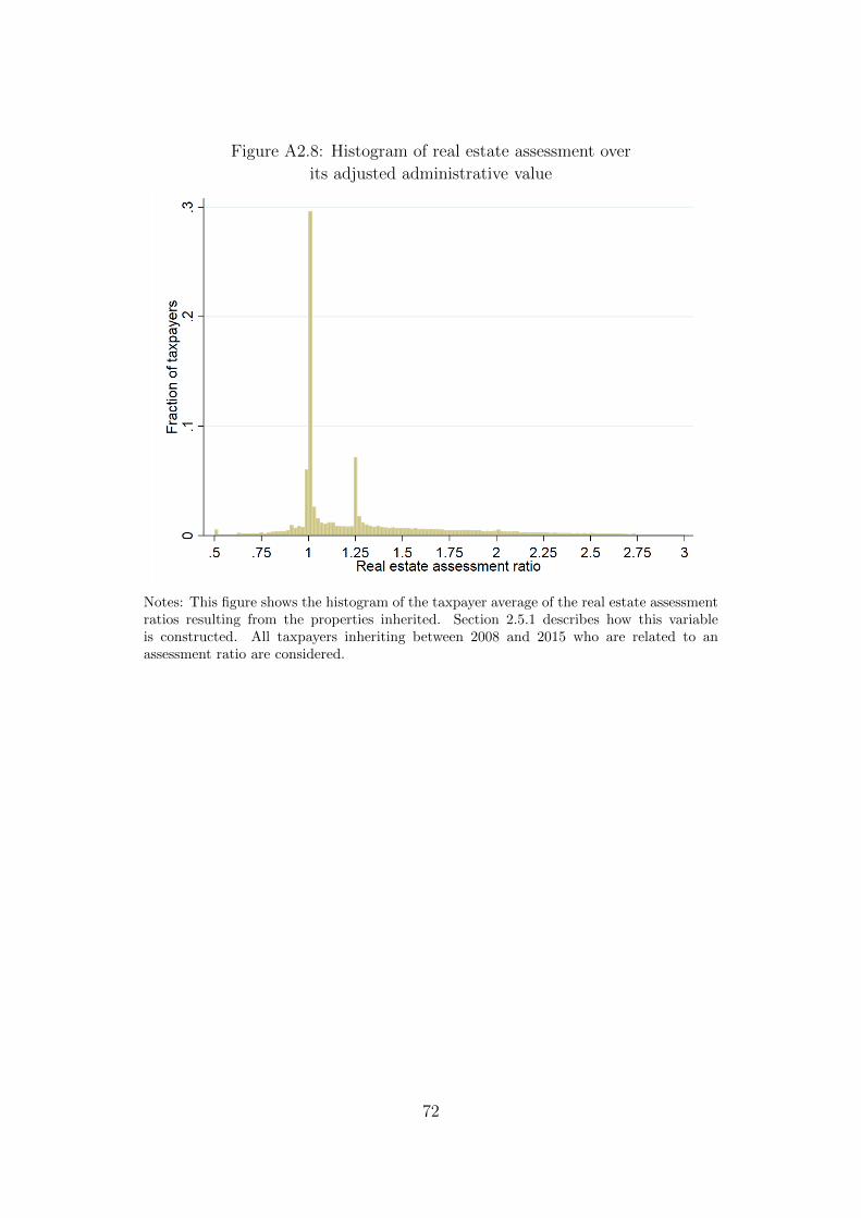
Figure A2.8: Histogram of real estate assessment over
its adjusted administrative value
Notes: This figure shows the histogram of the taxpayer average of the real estate assessmentratios resulting from the properties inherited. Section 2.5.1 describes how this variableis constructed. All taxpayers inheriting between 2008 and 2015 who are related to anassessment ratio are considered.
72

Figure A2.9: Net-of-“aggregate” marginal tax rates
Notes: This figure shows the evolution of the yearly averaged net-of-“aggregate” marginal tax rates(in logs) for treated and control groups, relative to 2010. Two different measures are used as the“aggregate” marginal tax rates: the panel on the left uses τAi , which is a weighted average of heirs’marginal tax rates according to their contribution to the aggregate tax base. The right-panel usesτMi , which reflects the higher marginal tax rate at which an estate is (partially) taxed. Section2.5.1 provides a more detailed definition of these measures.
73

Figure A2.10: Net-of-marginal tax rates
Notes: This figure shows the evolution of the yearly averaged net-of-marginal tax rates (in logs)for treated and control groups, relative to 2010. The left-panel considers all heirs included inthe treated and control groups. The right-panel only considers those heirs inheriting the largestportion of the estate.
74

Figure A2.11: Probability of reporting life insurance benefits
Notes: Both panels provide βy coefficient estimates and 95% confidence intervals resulting fromimplementing specification 2.3 for different treated groups. The dependent variable employed isa dummy which equals 1 if at least one heir reports life insurance benefits and 0 otherwise. Thenumber of observations of each type of estate in the percentiles 95-99 (top 1%) is: 11,913 (2,975)for all estates, 6,112 (1,436) for estates in which spouses do not inherit and 5,801 (1,539) for estatesin which spouses inherit.
75

Figure A2.12: Comparison of the baseline estimates with those obtained whenlife insurance benefits are included in the dependent variable
Notes: The panel in the left (right) provides βy coefficient estimates and 95% confidence intervalsresulting from implementing specification 2.3 for the treated group in the percentiles 95-99 (top 1%)of the distribution. Both panels compare the baseline coefficient estimates presented in Figure 2.6with those obtained when using the log of the aggregate tax base (i.e. estate + life insurancebenefits) as the dependent variable.
76

Figure A2.13: Comparison of the coefficient estimates obtained with the baseline vs. an alternative treatment definition
Notes: Each panel provides βy coefficient estimates and 95% confidence intervals resulting from implementing specification 2.3 for twoalternative definitions of treated and control groups. The baseline group definition is based on estates’ distribution. The alternative groupdefinition is based on the distribution of aggregate tax bases.
77

Figure A2.14: Effect of the 2011 tax cut on reported individual portions;distinction between estates inherited by spouses and estates which are not
Notes: Both panels provide βy coefficient estimates and 95% confidence intervals resultingfrom implementing specification 2.3 at heirs’ level for different treated groups. The depen-dent variable employed is the log of the individual portion inherited by each heir. Thenumber of observations of each treated group in the percentiles 95-99 (top 1%) is: 16,266(4,367) for estates in which spouses do not inherit, 9,929 (3,860) for estates in which spousesinherit less than 50% and 6,765 (1,413) for estates in which spouses inherit more than 50%.
78
Figure A2.15: Effect of the 2011 tax cut on the share inherited by each heir;distinction between estates inherited by spouses and estates which are not
Notes: Both panels provide βy coefficient estimates and 95% confidence intervals resultingfrom implementing specification 2.3 at heirs’ level for different treated groups. The depen-dent variable employed is the estate share inherited by each heir. The number of observationsof each treated group in the percentiles 95-99 (top 1%) is: 16,266 (4,367) for estates in whichspouses do not inherit, 9,929 (3,860) for estates in which spouses inherit less than 50% and6,765 (1,413) for estates in which spouses inherit more than 50%.
79

Figure A2.16: Effect of 2011 tax cut on reported estates; half-year estimates
Notes: The figure in the top panel shows the evolution of the half-year average of the (logof) reported estates, relative to the second half of 2010, for treated and control groups. Thefigure in the bottom panel provides βy coefficient estimates and 95% confidence intervalsresulting from implementing specification 2.3 with half-year dummies for both treated groupsand using the log of reported estates as the dependent variable. The number of observationsfor each group is: 9,879 for the control group and 11,913 (2,975) for the treated group inpercentiles 95-99 (top 1%).
80

Figure A2.17: Effect of 2011 tax cut on reported estates vs. “initial” estates
Notes: Both panels compare the baseline coefficient estimates presented in Figure 2.6 with thoseobtained when using the log of the initial estate (i.e. excluding the “added assets”) as the dependentvariable.
81

Figure A2.18: Comparison of the coefficient estimates obtained with the baseline vs. an alternative measure of reported assets;
Top 1%
Notes: Each panel provides βy coefficient estimates and 95% confidence intervals resulting from implementing specification 2.3 with the top 1%treated group. Two different measures of reported assets are used as the dependent variable: the log of Z1
i (baseline) and the log of Z2i (alternative).
Section 2.5.1 defines how these measures are constructed. Z = {real estate, financial assets, unlisted companies holdings and business assets,“unproductive” assets}.
82

Figure A2.19: Comparison of the coefficient estimates obtained with the baseline vs. an alternative measure of reported assets;
Percentiles 95-99%
Notes: Each panel provides βy coefficient estimates and 95% confidence intervals resulting from implementing specification 2.3 with the treatedgroup placed at the percentiles 95-99. Two different measures of reported assets are used as the dependent variable: the log of Z1
i (baseline) and thelog of Z2
i (alternative). Section 2.5.1 defines how these measures are constructed. Z = {real estate, financial assets, unlisted companies holdings andbusiness assets, “unproductive” assets}.
83

Figure A2.20: Comparison of the coefficient estimates obtained withthe baseline vs. an alternative measure of debts and deductible expenses
Notes: The left (right) panel provides βy coefficient estimates and 95% confidence intervalsresulting from implementing specification 2.3 with the treated group placed at the percentiles95-99 (top 1%). Two different measures of reported debts are used as the dependent variable:the log of Z1
i (baseline) and the log of Z2i (alternative). Section 2.5.1 defines how these
measures are constructed. Z = {debts and deductible expenses}.
84

Chapter 3
Avoidance Responses to the
Wealth Tax
3.1 Introduction
In the mid-eighties, about half the OECD countries imposed an annual net
wealth tax, but today it is maintained solely by Spain, Norway and Switzer-
land (OECD, 2018). However, rising wealth inequality1 has revived the debate
about the desirability of wealth taxes, not only in academic but also in po-
litical and public circles.2 To date, though, the empirical evidence about the
behavioural responses associated with wealth taxation, which might help an-
alysts form a well-grounded position on the need to implement such a tax
and on its appropriate design, is still limited (Seim, 2017; Brulhart et al.,
2017, 2019; Zoutman, 2018; Londono-Velez and Avila-Mahecha, 2019; Jakob-
sen et al., 2019).
The aim of this paper3, therefore, is to contribute to this nascent literature
by studying how taxpayers reacted to the reintroduction of the Spanish Net
Wealth Tax in 2011. We examine taxpayers’ responses in terms not only of
1Following Piketty (2014), several studies have attempted to estimate the evolution ofwealth concentration. Zucman (2019) provides a review.
2Clear evidence of this is the recent wealth tax proposal made by a US senator, Eliz-abeth Warren: https://www.warren.senate.gov/newsroom/press-releases/senator-
warren-unveils-proposal-to-tax-wealth-of-ultra-rich-americans.Evidence from the opposite camp comes from France, where the abolition of
the net wealth tax in January 2018 led to social unrest, its reinstatement be-ing one of the key demands of yellow vest protesters. See, for instance https:
//www.wsj.com/articles/france-could-keep-wealth-tax-in-bid-to-placate-
yellow-vests-1544025588; http://lavdn.lavoixdunord.fr/518614/article/2019-
01-09/le-ps-lance-une-plateforme-numerique-pour-pousser-son-retablissement
or http://piketty.blog.lemonde.fr/2018/12/11/yellow-vests-and-tax-justice/.3This paper is co-authored with Jose Marıa Duran-Cabre and Alejandro Esteller-More.
85

wealth accumulation, but also of the potential avoidance strategies adopted.
Spain provides a good setting in which to study the wealth tax given that it
is one of the few countries that continues to impose it. Moreover, behavioural
responses to wealth taxes in the country have not been previously examined.4
In Spain, wealth taxation has been transferred to sub-central governments,
who have the legislative power to determine certain aspects of its structure.
This is particularly relevant when we consider the reintroduction of the tax and
its implementation. For this reason, in this study we have opted to focus on
one of these sub-central governments (also for questions of data availability),
that of Catalonia, which is in fact the region that collects the highest share of
Spain’s overall wealth tax revenues (about 52% in 20115 and 46% in 20156).
Using a panel of tax return micro-data from the universe of Catalan wealth
taxpayers between 2011 and 2015, we analyse whether the wealth tax affects
wealth accumulation and taxable wealth. Additionally, we identify potential
avoidance strategies attributable to the design of the wealth tax, related pri-
marily to exemptions and the existence of a limit on tax liability. Specifically,
we examine whether taxpayers reorganize their wealth composition and change
the realization of income to benefit from them. Moreover, we also look at the
effect of the wealth tax on (reported) gifts. Finally, we seek to verify whether
there is a positive relation between wealth tax rates and the probability of a
taxpayer not filing wealth tax returns in subsequent years.
As there are no data for the period when the wealth tax was not being
imposed, we take advantage of the unexpected reintroduction of the tax by
the Catalan Government at the end of 2011. This serves as our control year.
We use the variation in treatment exposure, measured through the average
tax rates for 2011, to identify the effects of the wealth tax. This variation,
driven mainly by different ratios of taxable wealth over total reported wealth
and different shares of realized long-term capital gains over taxable income,
occurs not only across different levels of wealth, but also within similar levels.
Hence, we control non-parametrically for taxpayers’ 2011 wealth, income, asset
portfolio, age and other relevant characteristics.
4There exist other studies analysing the Spanish wealth tax (e.g. Alvaredo and Saez,2009; Duran-Cabre and Esteller-More, 2010) but they focus mainly on the evolution ofwealth concentration. Alvaredo and Saez (2009) also assess, at an aggregate level, theeffects of the introduction of business exemption.
5https://www.agenciatributaria.es/AEAT/Contenidos_Comunes/La_
Agencia_Tributaria/Estadisticas/Publicaciones/sites/patrimonio/2011/
jrubikf3a8b3676ae1f33ed00f20cdccba2a93cbf97232f.html6https://www.agenciatributaria.es/AEAT/Contenidos_Comunes/La_
Agencia_Tributaria/Estadisticas/Publicaciones/sites/patrimonio/2015/
jrubik53b6039ed4d69b32b967df1627a59aab8da95302.html
86

When focusing on a balanced panel of the top 50% richest taxpayers, our
results show that the taxpayers’ response to the reintroduction of the wealth
tax was significant. This translates into an elasticity of taxable wealth with
respect to the net-of-tax rate of return of 0.64, or, put differently, a 0.1 per-
centage point increase in the average wealth tax rate leads to a reduction in
taxable wealth of 3.24% over 4 years. This effect reflects avoidance rather
than real responses. Indeed, while facing higher wealth taxes does not have a
negative effect on savings, it does encourage taxpayers to change their asset
and income composition to take advantage of wealth tax exemptions (mostly
business-related) and the limit on wealth tax liability. The intensity of the
responses varies depending on the initial importance of taxpayers’ business
shares, favouring the use of business exemptions over the limit on tax liability
if initial business shares are high, and vice versa. Overall, these avoidance
responses are high in terms of revenues and increasing over time: in 2015
they account for 74.5% of 2011 estimated wealth tax revenues. Put differently,
the 4-year accumulated revenue loss amounts to 2.6 times the 2011 estimated
wealth tax revenues.
As such, this paper provides new empirical evidence to the nascent liter-
ature studying behavioural responses to wealth taxation. According to the
specific methodology applied, the existing literature can be divided into two
main groups: one employs bunching strategies (Seim, 2017; Londono-Velez and
Avila-Mahecha, 2019) while the other undertakes difference-in-differences and
cross-sectional analyses (Brulhart et al., 2017, 2019; Zoutman, 2018; Jakobsen
et al., 2019).7 The former report much smaller taxable wealth responses to
wealth taxes than the latter, primarily reflecting tax evasion.8 The mecha-
nisms driving such large responses in the latter studies are unclear.
Seim (2017) uses Swedish administrative data and exploits the variation
across wealth tax brackets, while Brulhart et al. (2019) use both aggregate
data at Swiss Cantons level and individual tax records for specific Cantons
and exploit the inter-cantonal time variation in wealth tax rates. Jakobsen
et al. (2019) employ Danish administrative data and consider two different
sources of variation: first, changes in the exemption threshold for couples and,
second, changes in marginal tax rates for taxpayers unbound by a tax ceiling.
Zoutman (2018) uses a Dutch capital-income and wealth tax reform that cre-
ated variation in the rate-of-return after taxation at each level of income and
7Note, however, that Brulhart et al. (2017, 2019) and Jakobsen et al. (2019) complementtheir main findings with bunching evidence.
8The specific magnitudes as reported in individual studies are detailed below in theResults section.
87
wealth and, finally, Londono-Velez and Avila-Mahecha (2019) draw on Colom-
bian administrative data and exploit the time variation derived from several
wealth tax reforms and discontinuities in the wealth tax schedule.
The main contribution of our paper - which by methodology belongs to the
second group of studies identified above - is that it provides both an assessment
of the effect of wealth taxes on taxable wealth and an analysis of other types
of response, focused above all on tax avoidance strategies, which allows us
to provide evidence of the mechanisms driving the results. Thus, the paper
also contributes to the literature on capital taxation and portfolio choice.9
While most earlier studies have sought to analyse the effect of personal income
taxes on investment in financial assets10, this paper provides evidence on asset
portfolio responses to wealth taxation, not only in terms of financial assets,
but also that of housing and businesses. On the one hand, higher tax rates
lead taxpayers to increase the importance of their exempt assets - in the main
their company holdings - although we also find a statistically significant (albeit
small) effect on their main dwelling exemption. This finding is in accordance
with the empirically documented use of closely-held businesses as tax shelters
(Alstadsæter, Kopczuk and Telle, 2014). On the other hand, higher tax rates
lead taxpayers to increase the importance they attach to listed equity and
investment funds, which enables them to exploit the tax liability limit.
Likewise, in relation to the application of this limit, our paper documents
that facing higher tax rates results in taxpayers reducing their taxable income
and increasing the importance of their long-term capital gains within realized
income. In this regard, our study contributes to the extant literature on the
responses of taxable income to personal income taxes (see Saez, Slemrod and
Giertz (2012) for a general review and Neisser (2018) for an empirical review)
and to the literature studying the effect of taxes on capital gains realizations11.
Finally, we provide evidence of gift responses to wealth taxes, which in turn
can be related to the literature studying the effect of gifts and estate taxation
9See Schalck (2017), Bergstresser and Pontiff (2013), Desai and Dharmapala (2011),Alan et al. (2010), Poterba and Samwick (2002). For a review of the earlier literature, seePoterba (2002).
10One exception is Bergstresser and Pontiff (2013), who also consider corporate incometaxation.
11Some recent empirical studies include Jacob (2018, 2016, 2013), Dıaz-Caro and Crespo-Cebada (2016) and Daunfeldt, Praski-Stahlgren and Rudholm (2010). In general, they studythe effect of capital gains taxation on their realization (also known as the lock-in effect) withthe exception of Jacob (2016), who studies the effect of labour income taxes on capital gainsrealizations. For a broad review of capital gains responses to taxes, see Hanlon and Heitzman(2010). With a particular focus on the wealthiest individuals, Auerbach, Burman and Siegel(2000) show that it is in fact the high-income, high-wealth and more sophisticated taxpayersthat are most likely to avoid capital gains taxation.
88

on inter-vivos transfers (see Kopczuk, 2017, for a review)12. Unlike the former
responses, the increase in - reported - gifts does not persist over time, only
being documented during the first two years after the reintroduction of the
tax.
The main conclusion we draw from this study is that the Spanish wealth tax
did not reduce wealth accumulation, and that the taxpayers most affected by
the reintroduction of the tax managed to reduce their tax liability significantly
by employing avoidance strategies. In addition, we find a positive relation
between the 2011 wealth tax rates and subsequent non-tax filing. Thus, in
broad terms, this paper contributes to the literature on capital and estate
taxation (see Kopczuk, 2017, for a review) and to that on tax avoidance and
evasion (Slemrod and Yitzhaki, 2002; Slemrod, 2018).
The rest of the paper proceeds as follows. Section 3.2 describes the specific
characteristics of the Spanish wealth tax and the circumstances surrounding
its reintroduction in 2011. Section 3.3 presents the data and descriptive statis-
tics. Section 3.4 outlines the methodology employed. Section 3.5 shows the
estimation results; and Section 3.6 concludes.
3.2 Spanish wealth tax: Evolution and char-
acteristics
The Spanish wealth tax was first introduced in 1977 as an extraordinary and
temporary measure, but after more than fifteen years the temporary nature of
the tax was revoked by Act 19/1991. Until that moment, the wealth tax had
mainly been used as an instrument for census and control purposes. However,
four additional objectives were pursued with the wealth tax reform: taxing
the additional ability to pay derived from wealth holdings; achieving a better
allocation of resources; serving as a redistributive tool and complementing
personal income tax and inheritance and gift tax.13
The wealth tax is levied annually on December 31 and applies to all forms
of wealth: real estate, bank accounts, bonds, shares, investment funds, life
insurance, vehicles, boats, aircrafts, jewellery, art and antiques, intellectual or
industrial property rights, etc. However, the legislation has incorporated a
number of exemptions: starting in 1991 with elements of historical heritage,
12In addition to studying the effect of estate and gift taxation on transfers, Joulfaian(2005) also considers the impact of capital gains taxation.
13Memorandum of Act 19/1991, June 6.
89

art treasures, pension plans and other financial rights14, wealth tax exemptions
were extended to business assets in 1994 and “closely-held” companies (both
unlisted - in 1994 - and listed - in 1998 -)15. Finally, main residences have been
exempt from the tax (up to a limit) since 2000.
The Spanish wealth tax is only levied on taxable wealth exceeding a mini-
mum threshold, a limit that has been modified over time. Wealth tax returns
have to be submitted in two different situations: (i) when taxpayers face a
positive tax liability, or (ii) when, although their tax liability is zero because
their taxable wealth is below the threshold, their gross wealth (including both
taxable and non-taxable assets) is above a certain level16. Tax liability is
obtained by applying progressive tax rates to the net tax base, i.e. taxable
wealth minus the minimum threshold. The wealth tax rates set by the Cen-
tral government range from 0.2 to 2.5%. Moreover, a limit exists on wealth
tax liability; specifically, the law sets a ceiling on wealth tax liability when
taxable income is relatively low compared to taxable wealth.17 It should be
noted that, although forming part of the legal definition of taxable income,
long-term capital gains (i.e. those derived from assets owned for longer than
twelve months) are excluded from the ceiling computations.18
Although the main structure of the tax continues to be regulated by Spain’s
Central government, since the mid-1980s, wealth tax revenues have been trans-
ferred to the regional governments. Some years later, they were also given
some limited legislative powers; thus, they can regulate the minimum thresh-
old, tax rates and tax credits. Additionally, they are also responsible for the
administration and control of the tax. This responsibility has been criticized
14Limited up to a certain amount. For further information, see Article 4, Act 19/1991.15Certain conditions must be satisfied for business assets and companies to be exempt
from the wealth tax. These requirements are not related to a firm’s size, but rather to aminimum ownership share (5% individually or 20% within the family group), a minimumremuneration for the performance of managerial duties (by at least one member of the familygroup) and the fact that the company carries out an economic activity. See Appendix 3.9.1for further information.
16Two million euros in 2011 and 601,012.10 euros in 2007.17This limit on wealth tax liability is not unique to the Spanish wealth tax. For instance,
in France, some Swiss Cantons (OECD, 2018) and Denmark (Jakobsen et al., 2019) haveoperated similar ceiling provisions. Indeed, Jakobsen et al. (2019) also exploit this taxfeature.
18Specifically, overall wealth and income tax liabilities cannot exceed 60% of taxableincome. The excess, if any, is deducted from the initial wealth tax liability. However, thisreduction cannot exceed 80% of the initial wealth tax liability. In short: Limited wealth taxliability=MAX(60% taxable income-income tax liability, 20% initial wealth tax liability), if[initial wealth tax liability + income tax liability]> 60% taxable income. Note that in thesecomputations, the sum of long-term capital gains and losses, if positive, is excluded fromtaxable income and the income tax liability needs to be adjusted accordingly.
90

for undermining the “control” function of the tax, given the difficulties en-
countered by the central and regional tax administrations to work together
(Duran-Cabre and Esteller-More, 2007).
In addition to the greater fraud risk associated with low rates of tax con-
trol (Duran-Cabre and Esteller-More, 2010), many experts have stressed the
inefficiencies and inequities derived from the design of this tax (i.e. assessment
rules that differ from market prices, tax exemptions, etc.).19 Apart from giving
rise to horizontal inequities among taxpayers with different asset portfolios but
with similar levels of wealth, its specific characteristics significantly distort the
incidence and redistributive role of the tax given that it is primarily the richest
taxpayers who benefit from them (e.g. Arcarons and Calonge, 2007; Alvaredo
and Saez, 2009).
Taking into account these limitations, at the end of 2008 the Central gov-
ernment decided to abolish the tax given its inability to meet the objectives
that justified its introduction in the first place.20
3.2.1 The reintroduction of the Spanish wealth tax
Surprisingly, the same Central government who suppressed the tax at the end
of 2008 decided to reintroduce it in 2011. The political party in power at that
time - the PSOE, occupying the centre-left of the political spectrum - opted
to implement the reform as a means of addressing the economic crisis. Its
argument was that those with more resources should be made to contribute
more to the economic recovery, and by so doing this would reinforce equity
and allow a better redistribution of income and wealth.
Thus, the tax was reintroduced in mid-September of 2011 as a transitory
measure and, a priori, it was only to be imposed in 2011 and 2012. How-
ever, the Budgetary Laws passed in subsequent years have each extended this
“transitory” measure and the Spanish wealth tax remains in force. Two main
changes were made with respect to the regulation applicable in 2007: (i) the
minimum threshold providing exemption from tax liability was raised from
108,182.1821 to 700,000 euros and (ii) the main residence exemption raised
19Enciso (2006), Duran-Cabre and Esteller-More (2007, 2014), Fernandez de Beaumontand Martın (2010), Carbajo (2015), among others.
20Memorandum IV of Act 4/2008, December 23. Due to legal constrains, the Wealth TaxLaw remained officially in force and Act 4/2008 simply introduced a 100% tax credit to thewealth tax liability.
21Regional governments have legislative capacity to fix a different minimum threshold.Before the abolishment of the tax, this ranged from 108,182.18 to 150,000 euros dependingon the region, where larger values were applied for specific situations.
91

from 150,253.03 to 300,000 euros. These changes sought to exempt the middle-
classes from paying the tax.
The reintroduction of the tax was characterised by the confusion to which it
gave rise right up to the very last moment. In July 2011, a prominent member
of the PSOE party - standing for election at the November polls but not a
member of the existing cabinet - proposed the introduction of a wealth tax
on the richest Spaniards as part of its manifesto. The proposal came under
heavy criticism from many sides, but above all from that of the centre-right
opposition party (PP), who expressed its dismay at the fact that it had been
the PSOE who had originally abolished the tax at the beginning of its mandate.
However, according to the opinion polls, the PSOE had lost support during
its second term in office to the PP22, who adopted a clear position against the
wealth tax. Thus, in summer 2011, the proposal to reintroduce the wealth tax
remained just that, a proposal.
Although the government ruled out any new tax reforms before the gen-
eral election23, rumours about an imminent reintroduction of the wealth tax
emerged in August 201124. The possibility was mentioned in various sources,
even making the front pages of several newspapers at the end of August25,26.
However, the Central government remained equivocal on the matter27. On
September 11, PSOE’s general election candidate called on the government
to reinstate the wealth tax, generating criticism across the board: Right-wing
parties condemned government inconsistency in relation to the wealth tax,
left-wing parties and organizations considered it an insufficient and belated
measure, and various groups of experts stressed the inefficiencies and limita-
tions of the tax.
The government failed to provide any specific details about the “new”
wealth tax until one day before its reintroduction28. On September 16, the
22In particular, according to voter intention surveys carried out by CIS (Centro de In-vestigaciones Sociologicas), PP became the most preferred political party to run the centralgovernment from mid-2010 onwards.
23http://www.europapress.es/economia/noticia-campa-descarta-nuevas-
reformas-fiscales-20110811104212.html24http://www.europapress.es/economia/fiscal-00347/noticia-economia-
gobierno-estudia-subir-irpf-antes-recuperara-patrimonio-consejo-general-
economistas-20110819183751.html25http://www.europapress.es/nacional/noticia-primeras-paginas-diarios-
llegados-noche-redaccion-20110823001848.html26http://www.europapress.es/nacional/noticia-primeras-paginas-diarios-
llegados-noche-redaccion-20110826002711.html27http://www.europapress.es/economia/noticia-salgado-no-aclara-si-piensa-
recuperar-patrimonio-20110823150753.html28http://www.europapress.es/economia/fiscal-00347/noticia-economia-ampl-
92

Council of Ministers agreed to its reinstatement and the legislation was mod-
ified accordingly29.
As discussed above, the wealth tax had been transferred to the Autonomous
Communities so it was they who would have the legislative power to decide
whether to levy it or not. Thus, even though the Central government had
approved its reintroduction, in the end it fell on the regional governments to
implement it or not. And, indeed, from the very outset, some of these gov-
ernments, including those of the Madrid Community and Catalonia, expressed
their disagreement with the measure.
Thus, the centre-right regional government in Madrid gave guarantees that
it would maintain the 100% tax credit introduced with the suppression of the
tax, while the centre-right nationalist Catalan government also expressed its
opposition to reintroducing the wealth tax, in line with the significant cuts to
the Catalan inheritance tax made earlier in June that same year. However,
with the reform passed, the Catalan government failed to legislate on the
actual implementation of the tax. Indeed, the Catalan government saw the
reform as a short-lived measure, given that the November General Elections
were close and all the indications were that the PP, who had come out against
the reintroduction of the tax, would be swept into power. This explains why
the Catalan government postponed its decision on the wealth tax until the new
Central government was formed.30
At the end of November 2011, the Catalan government announced that it
would, after all, levy the wealth tax, if the newly elected Central government
decided to retain it31, which turned out to be the case. It was not until mid-
December that the Catalan government confirmed that it would reintroduce
the tax in Catalonia, applying the same conditions foreseen in the state legis-
lation32, and it was not until March 2012 (with effect from December 31, 2011)
that it approved the corresponding legislative changes to implement the tax.
Consequently, Catalan taxpayers did not learn that they would have to pay
the wealth tax corresponding to 2011 until the end of that year, limiting their
recuperacion-patrimonio-sera-temporal-afectara-160000-contribuyentes-
aportara-1080-20110915132138.html29Real Decreto-ley 13/2011, de 16 de septiembre, por el que se restablece el Impuesto
sobre el Patrimonio, con caracter temporal.30http://www.europapress.es/catalunya/noticia-catalunya-aparca-decision-
impuesto-patrimonio-dudas-aplicacion-20110920154146.htm31http://www.europapress.es/catalunya/noticia-catalunya-no-subira-
impuestos-aplicara-patrimonio-si-pp-mantiene-20111122171408.html32http://www.europapress.es/economia/macroeconomia-00338/noticia-
economia-ampcataluna-estudiara-medidas-legales-reclamar-gobierno-759-
millones-disposicion-estatut-20111207103034.html
93

possibilities of responding to its reintroduction.33
Some months later, towards the end of September 2012, the Central gov-
ernment announced the extension of the wealth tax to 2013.34 Similarly, at the
end of September 2013, the government prolonged the tax again to 2014, and
so on, down to the present day. In Catalonia, at the end of 2012, the Catalan
government actually agreed to a slight increase in the wealth tax rates and
lowered the minimum threshold to 500,000 euros from 2012 onwards.35
3.2.2 How to avoid the Spanish wealth tax
Given the specific characteristics of the Spanish wealth tax, we need to com-
ment on the mechanisms that allow the tax liability to be reduced as this helps
explain the outcomes we present in our empirical analysis.
An obvious way to overcome the tax burden attributable to the progres-
sivity of the tax is by decreasing wealth. This can be achieved by making
gifts, although they are subject to gift taxes36. However, the design of the tax
allows taxpayers to adopt other strategies to reduce, or even eliminate, their
tax liability without decreasing their stock of wealth. Taxpayers do not even
need to hire a tax advisor - although many do - nor have a detailed knowledge
of Tax Law to learn about these strategies, as there are many explanations
and suggestions available on the internet.37
These strategies are related to reducing taxable wealth in favour of exempt
33There is anecdotal evidence in the form of readers’ letters to one of Catalonia’s leadingnewspapers complaining about the impossibility of making plans with respect to the wealthtax due to the lack of information and time constraints (see, for instance, La Vanguardianewspaper, November 28, 2011, p. 22, article ‘Hay que planificar’ ).
34http://www.europapress.es/economia/macroeconomia-00338/noticia-
economia-gobierno-crea-impuesto-loterias-prorroga-patrimonio-elimina-
deducciones-sociedades-20120927175205.htm35Statutory wealth tax rates were increased by 5%, except for the last tax bracket (net
tax base above 10.7 million euros) were the increase was 10%.36Gifts taxes depend on the family relationship between donor and recipient and on the
recipient’s region of residence. In Catalonia, for instance, tax rates range between 5-9% and11.12-64% for gifts to close and distant relatives, respectively. Additionally, in the case ofgiving real estate, the donor would face two taxes on capital gains (personal income tax anda local tax on urban land transmissions).
37Google provides 16.5M entries (April 10, 2019) when searching Como pagar menosimpuesto patrimonio (How to pay less wealth tax). Some examples are (websites inSpanish):https://www.consultingdms.com/impuesto-patrimonio-en-espana-10-formulas-
legales-para-evitarlo-o-reducirlo/;https://www.impuestosparaandarporcasa.es/2011/09/cuidado-con-lo-que-haceis-
para-no-pagar-impuesto-del-patrimonio;https://cincodias.elpais.com/cincodias/2016/10/13/abante_asesores/
1476347818_147634.html.
94

assets, making use of the limit on wealth tax liability or changing tax residence
to another region where the wealth tax is not levied (e.g. Madrid). Examples
for implementing the first option include: i) changing fiscal residence to that
of the dwelling with the highest assessment so as to take advantage of the
main-residence exemption38; ii) saving through pension plans; iii) investing in
art treasures; or iv) increasing business exemptions. The taxpayer can achieve
the latter by arranging their own businesses/shares in such a way that they
satisfy the exemption requirements foreseen in the Law (see Appendix 3.9.1). If
these conditions are already satisfied, the exemption value can be increased by
capitalizing the company, for instance. In the case of the first three examples
above, it should be stressed that their effectiveness for reducing taxable wealth
is limited, as exemptions are bounded39.
The alternatives for exploiting the limit on wealth tax liability are also
diverse. They require the taxpayer to reduce realized income and to invest
in assets that can generate long-term capital gains40. Both options can be
achieved by investing in investment funds, since these assets do not generate
regular income - such as dividends or interest - but only capital gains (or losses)
when sold. Shares are another type of asset that can help the taxpayer benefit
from the limit on tax liability.
Finally, the most radical strategy would be to move to Madrid. However, if
a tax audit were to be conducted the taxpayer would have to demonstrate that
this change of fiscal residence was neither fictitious nor motivated by reasons
of tax avoidance.
The most convenient strategy depends on the income-wealth ratio and the
asset portfolio of each taxpayer. For instance, for those who already own a
business it might be easier and less costly to take advantage of the business
exemption. Alternatively, those who have lower income and significant invest-
ments in financial assets might find it easier to benefit from the limit on tax
liability. Taxpayers with high income and high job mobility might consider
relocating to Madrid.
38This can only be done if the taxpayer owns several housing properties. According tothe Spanish Survey of Household Finances (wave 2011), 89% of individuals in the last decileof wealth distribution - that is, those most comparable to the population under study - ownother real estate properties besides their main dwelling (Banco de Espana, 2014).
39Main residence exemption is limited up to 300,000 euros. The yearly contribution topension plans was limited to 10,000 euros (12,500 euros for those older than 50). The ex-emption on art treasures depends on the type of asset and ranges from 2,404.05 to 90,151.82euros.
40As explained at the beginning of Section 3.2, long-term capital gains are excluded fromthe computation of the limit on wealth tax liability.
95

3.3 The data
The main data source used in this paper is the universe of anonymized wealth
tax returns filed by Catalan tax residents for the years 2011 to 2015. We
have complemented this database with an indicator of the taxpayer’s age and
information from inheritance and gift tax returns.41 All the data have been
provided by the Catalan Tax Agency.
The main database contains, at the micro level, all the information reported
in the wealth tax returns aggregated by types of asset. That is, the total stock
of wealth classified into real estate and main residence exemption, bank ac-
counts, business assets, bonds, investment funds, non-exempted quoted shares
and unlisted companies, exempted quoted shares and unlisted companies, life
insurance, vehicles, jewellery, artwork, property rights and “other”, including
all taxable wealth not previously categorized. Unfortunately, some exempt as-
sets such as historical heritage, art treasures and pension plans do not have to
be reported, which might underestimate the overall stock of taxpayers’ wealth.
Nevertheless, according to the Spanish Survey of Household Finances (SHF)
- wave 2011 - conducted by the Bank of Spain, assets of this type represent
a small fraction (around 4%) of households’ net wealth.42 Apart from wealth
portfolio, tax returns also include information on total taxable income and
personal income tax liability. Regarding personal characteristics, little infor-
mation is reported: just marital status and place of residence. As previously
mentioned, though, we are also able to consider age.
Table 3.1 provides descriptive statistics for 2011 wealth tax returns.43 Statis-
tics are provided by wealth deciles and total number of observations. Here,
certain features should be stressed: i) as total reported wealth increases, the
difference between taxable wealth and total wealth also increases; and ii) there
is significant variation in the average tax rate within the same wealth decile.
We return to this last point in the following section. Figure 3.1 shows the aver-
age asset portfolio, including all reported assets (both taxable and exempt), by
wealth deciles. The importance of unlisted companies increases with wealth,
while the reverse occurs with real estate properties and bank accounts or bonds.
The data from the 2011 tax returns submitted to the Catalan Tax Agency
41We are able to know whether a taxpayer dies after 2011 or has declared a gift from2008 onwards.
42This figure can be extracted from Table 2(cont.) and Table 4(cont.) from Banco deEspana (2014). We focus on the statistics for the last decile of the wealth distributionbecause it is the most comparable to the population under study.
43All wealth tax filers are considered, that is, those who face a positive tax liability andthose who must submit the tax return because their overall gross wealth exceeds 2 millioneuros, although their taxable base is below the minimum threshold.
96

show there were 42,294 tax filers facing a positive tax liability and 1,942 tax
filers with zero tax liability but gross wealth exceeding 2 million euros. Putting
the total number of tax filers - 44,236 - in perspective, they represent about
1.27% of personal income tax filers44 and about 0.59% of individuals residing in
Catalonia in 201145. Of these 2011 wealth tax filers, 36,373 (82.22%) continued
to submit a wealth tax return in 2015. Of the taxpayers who disappeared from
the sample (17.78%), 6.42% died and the remaining 11.36% disappeared for
other reasons (wealth losses, mobility, evasion, etc.). In our empirical analysis
we exclude those taxpayers that died. Additionally, we only consider those tax
filers who submitted the 2011 tax return, which means those taxpayers who
began to submit wealth tax returns later (from year 2012 onwards) are not
included in our study. In fact, most of our estimations use a balanced panel
of tax filers from the top 50% of the observed wealth distribution46, according
to the stock of wealth reported in 2011, who submitted wealth tax returns
consecutively between 2011 and 2015. We provide further details about this
in Section 3.4.
Finally, when a taxpayer voluntarily submits a supplementary return to
declare additional wealth, we consider this last return in our analysis. This
was a quite common occurrence among 2011 tax returns due to a tax amnesty
issued by the Central government in November 2012.47
3.3.1 Some descriptive facts on outcomes of interest
Table 3.2 shows the evolution taken by wealth tax revenues between 2011 and
2015. Values are expressed in 2011 prices. The figures shown in Table 3.2 only
consider those tax filers who submitted, at least, a 2011 tax return. In the
case of the 2011 wealth tax revenues, two different indicators are given: a) the
amount of revenues actually collected; and b) an estimation of the revenues
44Information obtained from the statistics published by the Spanish Tax Administration:https://www.agenciatributaria.es/AEAT/Contenidos_Comunes/La_
Agencia_Tributaria/Estadisticas/Publicaciones/sites/irpf/2011/
jrubik6ae6ffddfab109478ffa0128999b8085fe3b9c97.html.45Information obtained from the Catalan Statistical Institute: https://www.idescat.
cat/pub/?id=pmh&n=446.46We focus on the top 50% of the wealth distribution derived from the population under
study (i.e. wealth tax filers) not from the entire population.47The tax amnesty offered the possibility to regularize evaded income by paying a 10%
tax rate on the gross revenues generated during the non-prescribed years. Regularizationof income implied the declaration of wealth generating such income, and this is why manytaxpayers presented a supplementary wealth tax return. Indeed, 15.21% of 2011 tax filerssubmitted a supplementary 2011 wealth tax return around November 2012. See Chapter 4for further information on this tax amnesty.
97

that would have been collected if the tax changes approved in 2012 had already
been applied to 2011 wealth48. This estimation is provided to enable compara-
bility across years. A notable trend emerging from Table 3.2 is that wealth tax
revenues decreased by 19.23% between 2011 and 2015. When considering just
those taxpayers who submitted the tax return every year between 2011 and
2015, there was a fall of 3.64%. Revenues fell by 8.37% when considering that
group of taxpayers included in most of our estimations, i.e. those placed among
the top 50% of the observed wealth distribution filing wealth tax returns every
year. Another point that can be extracted from Table 3.2 is the importance, in
terms of revenues, of taxpayers who stop filing wealth tax returns. If we sum
all collected revenues (2011.a to 2015) for rows [1] and [2] we obtain 1,854M
and 1,680M euros, respectively. This translates into a wealth tax revenue loss
of almost 174M euros (expressed in 2011 prices) attributable to taxpayers who
no longer submitted wealth tax returns during the 2012-2015 period. Recall,
of these 174M euros, only 17.88% can be explained by taxpayers who died.
Table 3.3 provides some descriptive figures for the evolution of reported
wealth and tax avoidance strategies described in Section 3.2.2. All figures
refer to taxpayers placed at the top 50% of observed wealth distribution who
filed wealth tax returns every year between 2011 and 2015. Contrary to the
evolution of wealth tax revenues shown in row [3] of Table 3.2, overall reported
wealth increased during this period and, so, the latter does not seem to explain
the former. This in turn suggests there might be other factors, other than a fall
in the stock of wealth (such as the adoption of avoidance strategies), that are
driving the reduction in tax revenues. Indeed, a comparison of the 2011-2015
figures in Table 3.3 shows that the relevance of wealth exemptions, assets that
allow an investor to obtain long-term capital gains and the limit on wealth tax
liability have increased substantially over time.
In the case of the strategy of changing tax residence to another region,
the only information available to us thus far is that 11.36% of 2011 tax filers
disappeared from the sample in subsequent years for reasons other than death.
If we focus on the 50% richest, the share is similar, at 10.15%. When looking
at gifts reported to the Catalan Tax Agency, 5.92% of 2011 wealth taxpayers
(7.70% for those in the top 50%) made a gift between 2008 and 2011, when the
wealth tax was not in force. This share rose to 9.98% (14.26% for top 50%)
for gifts made between 2012 and 2015.
These are, nevertheless, merely descriptive facts. In the following sections
we consider the tax planning strategies explained above and examine the effect
48See Section 3.2.1 for further information regarding wealth tax changes.
98

of wealth taxes on wealth accumulation, on asset portfolio, on the probability
of making a gift, on taxable income and on other relevant outcomes.
3.4 Methodology
3.4.1 Measuring the impact of the reintroduction of the
wealth tax
As discussed, the objective of this paper is to study how taxpayers responded
to the reintroduction of the wealth tax in terms of wealth accumulation, wealth
composition and other outcomes we describe below. The ideal setting to carry
out this study would be that in which it was possible to compare - before and
after the reform - wealth taxpayers to similar individuals not subject to the
tax. However, this ideal control group does not exist. Therefore, instead, we
use as our identification strategy the variation in exposure to the treatment
(i.e. the reintroduction of the tax).
Figure 3.2, panel (a), shows the 2011 average tax rates, defined as the
wealth tax liability over total reported wealth, for different levels of wealth.
Additionally, it shows the highest average tax rate a taxpayer would face for a
given level of wealth, assuming all reported wealth is taxed (i.e. there are no
exemptions other than the minimum threshold of 700,000 euros that applies
to everyone) and the limit on tax liability is not operative.
Note that for a given level of wealth, some taxpayers face an average tax
rate close (or equal) to the maximum, whereas others face a much lower (or
even zero) average tax rate. In other words, taxpayers with similar levels
of wealth were differently affected by the reintroduction of the wealth tax.
This dispersion in tax rates originates from different sources: differences in
taxable wealth due to main residence and business exemptions and differences
in the tax liability when the limit applies. Using the average tax rate as a
measure of exposure to the treatment allows us to compile all these factors
into a single indicator. Figure A3.1 in Appendix 3.9.2 shows 2011 average tax
rates for different types of taxpayer: a) those for whom only the main-dwelling
exemption is applied, if any; b) those who also report business exemptions
(including both listed and unlisted companies); c) those who qualify for the
limit on tax liability and d) those who satisfy both b) and c). Most of the
variation in the tax rates originated from situations b), c) and d), given that
the main-dwelling exemption is bounded up to 300,000 euros.
Figure 3.2, panel (b), shows an estimation of the average tax rates that
99

taxpayers would have faced in 2011 if the wealth tax changes approved in
2012 had been applied in the previous year. The picture does not change
greatly from panel (a). This is the case because, again, tax changes would
differently affect taxpayers with similar levels of wealth due to the existence of
wealth tax exemptions and the limit on wealth tax liability. Therefore, both
indicators (real and estimated average tax rates) provide very similar measures
of taxpayers’ exposure to the wealth tax.
Part of the literature uses marginal tax rates to analyse responses to tax
rate variations49, usually in the last tax bracket. However, it is not the aim of
this paper to study responses to changes in top marginal tax rates. It seeks to
study responses to a tax reintroduction, which implies tax changes for all tax
bases exceeding the minimum threshold. In this context, we believe marginal
tax rates to be a less precise measure of treatment intensity, especially for
the wealthiest. This is the case because tax brackets are wide50 and, thus,
taxpayers with different tax liabilities may face the same marginal tax rate.
Therefore, for the case under study we consider it more appropriate to use
average rather than marginal tax rates as our explanatory variable.51
Returning to Figure 3.2, it is evident that the variation in tax rates increases
with wealth and that it is quite low for the bottom 50% of the observed wealth
distribution. Precisely because our identification strategy relies on the varia-
tion in treatment exposure, henceforth we focus our analysis on the top 50% of
the observed wealth distribution. In fact, according to the figures provided in
Table 3.2, the bottom 50% only accounts for a small part of the 2011 collected
wealth tax revenues, so the potential responses we fail to estimate should have
little impact in terms of revenues.
Using the 2011 average tax rates as our explanatory variable has, therefore,
the advantage of providing an accurate indicator of the treatment exposure,
but it also has a drawback: it depends on taxpayers’ 2011 wealth, income
and asset portfolio. To deal with this issue, we control non-parametrically for
taxpayers’ 2011 wealth, income, asset portfolio, age and other characteristics
that might influence our dependent variables (see the following section for
further details).
49See, for instance, Saez, Slemrod and Giertz (2012) for a review on the elasticity oftaxable income.
50Table A3.1 in Appendix 3.9.2 shows the statutory tax rates in Catalonia for 2011.51An alternative explanatory variable could be an average tax rate expressed in terms of
income rather than wealth. However, we believe the average tax rate expressed over wealthto be more accurate. Some taxpayers in our data misreport information on income and,additionally, wealth is a stock whereas income is a flow, which is more likely to fluctuateand, so, provide a distorted indicator.
100

3.4.2 Measuring behavioural responses to the reintro-
duction of the wealth tax
Unfortunately, we have no information on taxpayers’ wealth for the period
when the wealth tax was not in force, as it was simply not being collected.
However, taking into account the largely unexpected and belated reintroduc-
tion of the tax in Catalonia (see Section 3.2.1), we argue that 2011 can serve
as a control year.
This assumption is further reinforced by the fact that wealth is a stock,
which is not easily adjusted instantaneously, and in any case, such adjust-
ments are costly. The initial short-term duration of the measure (just 2 years)
increased these adjustment costs. Moreover, as discussed in Section 3.2, the
assessment rules do not always coincide with the market value, but depend on
specific criteria, a situation that complicates the asset valuation adjustment.
For instance, wealth deposited in bank accounts is valued at the highest of
the 4th quarter average balance or the balance at December 31. For quoted
shares and quoted bonds, the 4th term average value is also used. Banks and
investment entities do not provide their customers with all this information
until the first quarter of the following year when they have to file their income
and wealth tax returns. Unlisted companies are assessed according to the book
value obtained from their last audited balance sheet, i.e. 2010 balance sheets
for the 2011 wealth tax returns. In the case of real estate, this is not assessed
according to its market price either, but by the highest between its cadastral
and acquisition values.
The central tax administration automatically receives information on real
estate and financial assets. In this sense, it is difficult for taxpayers to hide
wealth of this kind. The situation is obviously different for “unproductive”
assets, such as antiques or jewellery, and indeed very few tax filers report
this type of wealth. In any case, according to survey evidence, this wealth
represents a very small fraction of taxpayers’ total worth.52
While we cannot directly test the assumption that taxpayers were largely
unable to react to the reintroduction of the wealth tax in 2011, we can inspect
related indicators such as gifts. This is a rapid and effective manner of reducing
wealth. Thus, if taxpayers had made a concerted effort to rapidly reduce their
wealth at the end of 2011, we should observe a spike in the number of gifts
declared during that period. However, gifts data suggest this not to be the
52According to the Spanish Survey of Household Finances (wave 2011), jewellery, worksof art and antiques represent around 0.9% of net wealth for the last decile of the wealthdistribution, i.e. the one most comparable to the taxpayers under study here.
101

case. Figure A3.2 in Appendix 3.9.2 shows the frequency of gifts declared in
Catalonia during the last 8 weeks of every year between 2009 and 2014. Gifts
declared during the last 8 weeks of year 2011 are no higher than in previous
years, when the wealth tax was not in force.
In any case, we do not need a complete lack of response in 2011 for our
identification strategy. What we, in fact, require is that, after controlling for
2011 reported wealth, income, asset portfolio, age and other personal char-
acteristics (see below), taxpayers are comparable and would behave alike in
the absence of the wealth tax. This requires a similar reporting (and under-
reporting) behaviour among similar taxpayers based on their 2011 tax returns.
In the case of significant under-reporting behaviour in 2011 due to the rein-
troduction of the wealth tax (which we consider implausible for the reasons
outlined above)53, the responses we estimate would be a lower bound.
The empirical specification we implement is the following:
Dep.vari,t =∑
y 6=2011
αy · Yy=t · atr11i + γt + δi +∑
y 6=2011
λy · Yy=t ·X11i + νi,t (3.1)
where Dep.vari,t is one of the dependent variables that we explain below,
Yy=t is a year dummy that takes a value of 1 when the year equals t, atr11iis 2011 average tax rates, αy is our parameter of interest54, γt captures year
fixed effects, δi is an individual fixed effect and X11i is a set of non-parametric
controls detailed below and based on the reference year, 2011. In the case of
atr11i , we use both the real and the “estimated” 2011 average tax rates shown
in Figure 3.2.
The dependent variables we examine are: log of taxable wealth, log of total
reported wealth, log of taxable income, the probability of making (and declar-
ing) a gift55, the probability of facing the limit on tax liability56, the share of
long-term capital gains over taxable income, the share of exempt assets over
total reported assets and different components of taxpayers’ asset portfolio;
specifically, the share of (i) real estate; (ii) business assets and unlisted com-
panies; (iii) listed equity and investment funds; and (iv) bank accounts and
bonds, distinguishing between exempt and taxable assets. Indeed, we are in-
terested in the evolution of these variables with respect to the base year; hence,
53Here, we do not consider offshore evaded wealth, which would not have been reportedeither in the absence of the wealth tax due to the existence of income taxes.
54We later relate this coefficient to elasticities with respect to the net-of-tax rate of return.55We define a dummy which takes a value of 1 if a taxpayer makes a gift in year t (and
it is reported to the Catalan tax authorities), and 0 otherwise.56We define a dummy which takes a value of 1 if a taxpayer faces the limit on tax liability
in year t, and 0 otherwise.
102

the estimates are normalized with respect to 2011. Given that the type and
magnitude of the responses might vary depending on the initial wealth compo-
sition, we examine heterogeneous effects according to the relative importance
of unlisted companies and business assets over total reported assets in 2011.
We also show the estimation results from specification 3.1 without including
the set of non-parametric controls X11i interacted with year dummies Yy=t. To
be able to talk about causal effects, the underlying assumption behind this
specification would require that wealth components evolved in the same way
for all taxpayers in the absence of the wealth tax, once time and individual
fixed effects have been taken into consideration. However, we consider this
a strong assumption to make, especially because we cannot test it, given the
absence of data for the period when the wealth tax was not in force. For this
reason, we include the control variables defined below.
To capture non-tax trends driven by changes in asset prices and asset-
specific returns57, we create deciles of the following asset shares: i) housing;
ii) listed equity and investment funds; iii) unlisted companies and business
assets; and iv) bank accounts and bonds. Since we only have information
on overall taxable income, but not on capital income specifically, we control
both for taxable income58 and wealth deciles to further address differences in
returns, given that there is evidence of a positive correlation between returns
and the level of wealth (Fagereng et al., 2018). Additionally, controlling for
income and wealth levels avoids mean reversion issues. To deal with differences
in saving rates and attitudes towards inheritance and gift tax we control for
age groups with the following cut-offs: 45, 65 and 75 years.59 To further
control for differences in saving rates we also include deciles of the share of
debt over total assets. All these control variables are defined according to
the information reported in 2011 wealth tax returns and interacted with year
dummies Yy=t. Finally, as the tax amnesty mentioned in Section 3.3 took
place during the period under study, this might have affected the reporting
behaviour from 2012 onwards. Thus, we also include a dummy indicating tax
amnesty participation interacted with year dummies.60 For reference purposes,
57Considering the specific assessment rules provided in the Wealth Tax Law, changes inasset prices might not necessarily be reflected in tax returns (for instance, those relatedto real estate). However, changes in asset returns might affect taxpayers’ investment andsaving behaviour.
58We define an extra category for those taxpayers who do not report information onincome (representing 10% of the observations used in the main estimations). We also checkedthat our results do not substantially change when excluding these observations; they do not.
59We define an extra category for those taxpayers whose age is non-available (representingjust 0.06% of the observations used in the main estimations).
60We do not know exactly whether a taxpayer participated in the tax amnesty or not,
103
we define this set of controls as “decile controls”.
Constrained by the fact that we cannot test the parallel trends assump-
tion, we also use an alternative set of non-parametric controls including the
same variables detailed above, but defined more narrowly to reduce the cor-
relation between 2011 average tax rates and 2011 taxpayers’ wealth, income
and asset portfolio. In particular, wealth and income are ranked every 5 and 4
percentiles, respectively. Asset shares are ranked every 2.5 percentage points,
with the exception of housing shares, which are ranked every 2 percentage
points. The remaining variables have the same definition as above. Again, all
the control variables are defined according to the information reported in the
2011 wealth tax returns and interacted with year dummies Yy=t. For reference
purposes, we define this set of controls as “narrow controls”.
Table A3.2 in Appendix 3.9.2 shows the relation between 2011 average tax
rates and 2011 taxpayers’ wealth, income and asset portfolio when no controls
are included and when “decile” and “narrow” controls are considered.
In summary, for each dependent variable we show three different estimates:
a- Those obtained when controlling only for time and individual fixed ef-
fects.
b- Those obtained when using the “decile controls” as X11i .
c- Those obtained when using the “narrow controls” as X11i .
Next, we need to address the potential mechanical effect of taxes on wealth.
If taxes are paid out of savings, then they mechanically reduce wealth, even
in the absence of behavioural responses. In order to account for this potential
mechanical effect, we adjust yearly reported wealth and taxable wealth with
the wealth tax liabilities paid up to that date by applying a 3% net rate of re-
turn.61,62 The mechanical effect, however, would not be present if wealth taxes
were paid through consumption, substituting other expenditures for such pay-
ments. Since we have no information to test these hypotheses, our results for
but we can identify those taxpayers who submitted a 2011 wealth tax form when the taxamnesty took place (October-November 2012); time in which the voluntary period hadalready expired. Therefore, we consider as tax amnesty participants those taxpayers whofiled a 2011 wealth tax form during, or later than, October 2012.
61Assuming that wealth taxes are paid out of financial assets, we compute an average grossrate of return to financial assets using the 2011 Survey of Household Finances microdata.This average is 4% for households whose net wealth is above 1.5M euros (this is the lowestnet wealth value in our estimation sample). In turn, we compute the net rate of returnapplying capital income tax rates (25% for years 2012-2014 and 21.5% for 2015).
62For instance, 2012 reported wealth is adjusted with (2011 wealth tax liability)*1.03.Successively, 2013 reported wealth will be adjusted with (2011 wealth tax liability)*1.032
and (2012 wealth tax liability)*1.03, and so on.
104

taxable and total reported wealth are presented both omitting and adjusting
for the mechanical effect. Results concerning wealth composition, though, only
provide overall effects (behavioural + mechanical, if any), since we would need
to make strong assumptions about the specific assets used to pay wealth taxes
to adjust for the mechanical effect.
3.4.3 Further discussion of the identification assump-
tions
We would like to make clear where the variation in average tax rates comes
from, after including the set of non-parametric controls. The answer is from
the exemptions and the limit on tax liability. Thus, while we control for
the overall housing, listed equities and unlisted companies share, the specific
importance of the exemptions within these shares varies across taxpayers. For
instance, imagine two identical taxpayers with just one difference: taxpayer Z
owns 4% of two different unlisted companies and taxpayer S owns 6% and 2%,
respectively. The overall value of these assets is the same for both taxpayers;
nevertheless, taxpayer S can exempt part of these shares from the wealth tax
whereas taxpayer Z cannot, as his ownership share is below 5%63. Consider
now two other identical taxpayers with just one difference: taxpayer X owns
a very expensive main dwelling, while taxpayer Y owns a small main dwelling
and a second residence. The overall value of these assets is again the same
for both taxpayers. However, taxpayer X will face a lower average tax rate
than taxpayer Y, given that only main-dwellings are exempt from the tax,
up to 300,000 euros. Because of the existence of this limit, the variation
originating from the main-dwelling exemption is also limited. The last source
of variation comes from the importance of long-term capital gains in taxable
income. To illustrate this, imagine two identical taxpayers who sell the same
shares, obtaining the same capital gain. However, one of them purchased the
shares 2 months earlier than the other and so the gains qualify as long-term,
whereas the others do not. The first taxpayer faces the limit on tax liability;
the second does not. Table 3.4 shows the relation between 2011 average tax
rates and each particular source of variation, once controlling for the “narrow”
set of non-parametric variables.
The underlying assumption behind these examples and the specification
employed is that, once controlling for time and individual fixed effects and the
set of controls detailed above, the specific importance of the exemptions and
63A minimum 5% ownership share is one of the requirements to exempt business assetsand holdings from the wealth tax. For further information, see Appendix 3.9.1.
105
long-term capital gains would not affect the evolution of reported wealth and
its components in the absence of the wealth tax. Unfortunately, we cannot
demonstrate this, because, again, there are no data for the period when the
wealth tax was not in force, but below we provide some arguments that should
help to validate this assumption.
First, the exemption status for companies, both listed and unlisted, and
for business assets is simply a legal definition included in the Wealth Tax Law.
The conditions required by the Law to apply this exemption do not depend on
a firm’s characteristics or outputs, such as number of employees, sales volume,
productivity indices, profits, etc., but rather on ownership share.64 Moreover,
there is no public register or list of companies potentially exempt from the
wealth tax, so there is no way for them to be readily identified. Indeed, pre-
cisely because exemption status depends on ownership share, the same com-
pany might be exempt for one taxpayer and non-exempt for another. It is
the individual taxpayer that is able to accredit their exemption with regard to
their own shares, not the company itself. Finally, the definition of exemption
included in the Wealth Tax Law is not used in any other domain, except that
of the inheritance tax. Close heirs who inherit company shares that may be
exempt from the wealth tax can apply a tax deduction on the inheritance tax.
Therefore, besides the wealth tax, this exemption could be important for old
wealth taxpayers. Given that we control for taxpayers’ age this should not be
an issue. Moreover, the Catalan government practically eliminated the inher-
itance tax for close inheritors in June 201165, a fact that virtually eradicates
the importance of this deduction.
In the case of the main-residence exemption, it is difficult to see why the
relative importance of the value of this asset in relation to that of other resi-
dences should affect the evolution of reported wealth and its components, once
housing shares, income and the set of controls described above have been taken
into account. In relation to long-term capital gains, they are taxed at the same
rates as financial capital income in personal income tax; thus, a priori there is
no clear tax incentive, besides that of the wealth tax, to prioritize long-term
capital gains realizations over other sources of capital income.
Finally, we should stress that we are focusing on the evolution of 2011
reported wealth and its components. It lies beyond the scope of this paper
to evaluate the wealth already evaded in 2011. Nevertheless, as explained
64The Law also requires that at least one member of the family group performs remuner-ated management functions within the firm. See Appendix 3.9.1 for more details.
65The Catalan government introduced a 99% tax discount for close inheritors and, con-sequently, tax rates ranged between 0.07 and 0.32%. See Chapter 2 for further information.
106

at the beginning of this section, we do not need to assume that there is no
evaded wealth for our identification strategy to hold. This strategy relies on the
comparability of taxpayers according to the information reported in the 2011
wealth tax returns, meaning it assumes that their reported wealth, income
and asset portfolio would evolve similarly in the absence of the wealth tax,
conditional on the set of control variables and fixed effects already explained.
In turn, this assumption implies that the presence of evaded wealth should
not affect differently the evolution of the reported variables during the period
under analysis, once all the controls and fixed effects are taken into account.
Evaded wealth should be related in the main to unproductive assets, such as
jewellery or antiques, and to offshore accounts. The former do not generate re-
turns and, as we have seen, represent a very low fraction of individuals’ wealth,
so they should not be an issue for our identification strategy. In the case of
offshore accounts, it is difficult to identify a channel via which wealth held
in tax havens could affect the evolution of reported assets, besides taxpayers’
attitudes towards risk and other “evader” characteristics, which would be cap-
tured by individual fixed effects, or global economic circumstances, captured
by year fixed effects.
3.4.4 Extensions and general methodological comments
Finally, we check whether treatment exposure is related to the probability
of disappearing from the sample. To do this, we implement the following
specification:
Disappeari = γ + α · atr11i + λ ·X11i + νi (3.2)
where Disappeari is a dummy which takes a value of 1 if a taxpayer who sub-
mitted a 2011 tax return subsequently disappears from the sample for reasons
other than death. Alternatively, it takes a value of 0 for taxpayers who filed
wealth tax returns every year between 2011 and 2015. The explanatory vari-
able, atr11i , is the 2011 average tax rate, α is our parameter of interest and
X11i is a set of non-parametric variables which include the “decile” or “narrow”
controls defined above and two additional dummies which identify married tax
filers and those who live in the province of Barcelona.66 In contrast to speci-
fication 3.1, we are not able to capture unobserved individual characteristics;
hence, the estimation results from specification 3.2 need to be treated with
66These two additional dummies are captured by individual fixed effects in specification3.1.
107

caution.
Before moving to the results, some additional methodological comments
need to be made. First, all monetary values are expressed in 2011 euros and,
second, standard errors are clustered by the married taxpayers identified in the
sample. This is the case when they submit income tax returns jointly; however,
they have to submit their wealth tax returns individually so as to report their
own wealth. Finally, to deal with outliers, taxpayers placed in the top 0.5%
of reported wealth and taxable income distributions are not considered in the
estimations.
3.5 Results
3.5.1 Main analyses
Figures 3.3-3.11 show the coefficient estimates and 95% confidence intervals
resulting from specification 3.1 for the multiple outcomes previously specified.
Each figure provides three different sets of estimates: a) those obtained when
controlling only for time and individual fixed effects (controls -a-); b) those
obtained using the “decile controls” asX11i (controls -b-); and c) those obtained
using the “narrow controls” as X11i (controls -c-). Estimations have been
carried out using both the real and the “estimated” 2011 average tax rates
as the explanatory variable; however, as they give very similar results, we
only discuss the estimates obtained with the real average tax rates. Results
obtained with the “estimated” average tax rates are provided in Appendix
3.9.3.
In the case of the coefficient estimates from year 2013 onwards, we are
unable to disentangle which part of the response can be attributed to the
wealth tax reintroduction per se and which to the tax increase approved at
the very end of 2012.67 In any case, we are interested in the overall responses,
even if the tax was implemented in two different steps.
Taxable and reported wealth responses
Figure 3.3 shows the coefficient estimates from specification 3.1 when consid-
ering taxable wealth. The panel to the left shows overall effects (behavioural
67The coefficient estimates for 2012 can be fully associated to a response to thewealth tax reintroduction. The 2012 wealth tax increase was passed on Decem-ber 27, 2012 and until a few days before its approval had not been previouslydiscussed. See: http://www.europapress.es/catalunya/noticia-govern-reforma-
impuesto-patrimonio-ingresar-70-90-millones-extra-20121227215328.html.
108

+ mechanical, if any), while the panel to the right shows behavioural effects,
since taxable wealth has been adjusted for the mechanical effect, assuming in
this case that wealth taxes are paid out of savings. The estimates obtained are
very similar when using “controls -b-” and “controls -c-”, which is also the case
for most of the outcomes studied. Thus, the small differences in 2011 levels
when using the set of “decile” controls do not seem to matter when accounting
for the trends. The estimates obtained when controlling only for individual
and time fixed effects, controls -a-, are smaller (in absolute values), but follow
a similar pattern.
The “control -c-” estimates, resulting from our preferred specification, re-
flect a negative effect of treatment exposure on taxable wealth accumulation.
The response is already statistically significantly different from zero in 2012
and accumulates over time. The coefficient estimate associated with year 2012
suggests that as the 2011 average tax rate increases by 1 percentage point, tax-
able wealth lowers by 15.34%. This decrease accumulates to as much as 32.44%
over 4 years. If we adjust taxable wealth with the (assumed) mechanical ef-
fect, the 2015 coefficient becomes -29.08%, suggesting that the behavioural
(mechanical) effect accounts for 89.65% (10.35%) of the overall effect.
To interpret the coefficients, note that a 1 percentage point increase in the
average tax rates represents a large experiment: applying it to the mean of
2011 average tax rates for the estimation sample, which is 0.30%, it would
represent a tax increase of more than three times. For this reason, from now
on we refer to the estimates in terms of a 0.1 percentage point increase.68
The coefficients obtained are within the range reported in the extant litera-
ture on wealth taxes. However, the comparison that follows should be treated
with caution, since tax base definitions and the overall design of the tax vary
across countries (for a summary of OECD cases see OECD, 2018) and they
might determine the responses estimated - besides other factors such as tax
morale or tax enforcement -.
Among the studies that employ similar methodologies to the one used here,
the lowest estimate is reported by Zoutman (2018), who finds that a 0.1 per-
centage point change in the wealth tax reduces accumulated taxable wealth
by 1.16% in the short-run (over 2 years) and 1.38% in the long-run (over 5
years). These estimates rise to 1.3 and 1.67%, respectively, when the author
looks at households above the 75th wealth percentile, a sample that might be
more comparable to ours. Yet, our 2-year estimate (-2.25%) is still higher.
Jakobsen et al. (2019) report an increase of taxable wealth of about 30% over
68This is also the approach followed by Brulhart et al. (2017) and Zoutman (2018).
109

8 years for the top 1% of the wealth distribution, in response to an average
tax cut of 1.56 percentage points. This estimate is almost 20% in the 4th
year after the reform, which is also lower than our 4th-year coefficient. Using
cross-canton data Brulhart et al. (2019) estimate that a 0.1 percentage-point
rise in wealth taxes lowers reported wealth by 4.1% over 4 years. The stud-
ies employing bunching techniques - that is, Seim (2017) and Londono-Velez
and Avila-Mahecha (2019) - report much lower estimates: a decrease in tax-
able wealth of 0.027% and 0.2%, respectively, if we interpret the coefficients in
terms of a 0.1 percentage point increase in the wealth tax rates.69
Following the reasoning of Brulhart et al. (2017), we next express our coef-
ficient estimates in terms of the implied net-of-tax rate on the annual returns
to wealth. The mean of the average income (wealth) tax rates in 2011 is 24%
(0.30%) for the estimation sample. Considering a gross rate of return to net
wealth of 3%, computed from the 2011 Spanish Survey of Household Finances
microdata70, the mean average wealth tax rate corresponds to a 10% tax on
capital return. Hence, the net-of-tax rate, considering both income and wealth
taxes, is 1-(0.24+0.10)=66%. A 0.1 percentage point increase in the wealth tax
represents a 3.33 percentage point increase in the tax on capital return, which
leads to a net-of-tax rate of 1-(0.24+0.1333)=62.67%. Thus, a 0.1 percentage
point increase in the wealth tax, which translates to a reduction of 5.05% in
the net-of-tax rate, lowers accumulated taxable wealth by 3.24% over 4 years.
Therefore, the elasticity of taxable wealth with respect to the net-of-tax rate
of return is 3.24%/5.05%=0.64. Comparable estimates from other studies in
the wealth taxation literature take values of 1.05 in Brulhart et al. (2019),
0.5 in Jakobsen et al. (2019)71 and 0.08 in Londono-Velez and Avila-Mahecha
(2019). Nevertheless, it should be noted that these estimates are sensitive to
the assumed rate of return, as shown in Brulhart et al. (2017, 2019).
Figure 3.4 shows the coefficient estimates from specification 3.1 when con-
69The estimates in Seim (2017) and Londono-Velez and Avila-Mahecha (2019) are notdirectly comparable because they account for the elasticity of taxable wealth with respectto the net-of-wealth tax rate. Nevertheless, taking into account that wealth tax rates arelow (1.5% in Seim 2017 and 1% for the first 2010 tax bracket in Londono-Velez and Avila-Mahecha 2019), we can use the property of logarithms: log(1+x) ≈ x, for small x, to expressthe estimates in terms of a 0.1 percentage point change in the wealth tax rates. Consideringthe upper-bound estimates in both cases, the comparable coefficients are -0.027 and -0.2,respectively.
70We compute an average gross rate of return to net wealth using the 2011 Survey ofHousehold Finances microdata. This average is 3% for households whose net wealth isabove 1.5M euros (this is the lowest net wealth value in our estimation sample).
71Elasticity computed for the top 1% of the wealth distribution over an 8-year period.The change in the net-of-tax rate of return is 61% and the accumulated effect on taxablewealth is about 30%.
110

sidering total reported wealth. As in Figure 3.3, the panel to the left shows
overall effects (behavioural + mechanical, if any), while the panel to the right
shows behavioural effects, assuming the mechanical effect takes place. Inter-
estingly, wealth taxes do not have a negative effect on wealth accumulation.
Estimates from the left-hand panel suggest that wealth taxes do not have a sig-
nificant impact on the evolution of total reported wealth. If we assume wealth
taxes are paid out of savings (thus, mechanically reducing wealth), when we
account for this effect in the right-hand panel, the estimates indicate that the
taxpayers that are most exposed to the reintroduction of the tax increase their
savings in the subsequent years. Specifically, as the 2011 average tax rate
increases by 0.1 percentage point, reported wealth increases by 0.5% over a 4-
year period. If we translate this estimate into an elasticity with respect to the
net-of-tax rate of return following the same procedure as described above, it
takes a value of -0.1. There could be several explanations for this: i) taxpayers
derive some utility from wealth per se, also known as “capitalistic spirit” mo-
tive (see Kopczuk, 2010; Saez and Stantcheva, 2018) and, hence, they increase
their savings to offset the mechanical effect of wealth taxes; and ii) taxpayers
make use of tax avoidance strategies and defer the realization of capital income
to take advantage of the limit on tax liability. The following sections seek to
shed further light on this.
Avoidance responses
Figure 3.5 shows the coefficient estimates from specification 3.1 when consid-
ering potential tax avoidance strategies derived from the design of the wealth
tax. As explained in Section 3.2.2, these strategies are related to the use of the
limit on wealth tax liability and exempt assets. The left-hand panel shows a
positive relationship between exposure to the reintroduced tax and the proba-
bility of facing the limit on wealth tax liability in subsequent years. Taxpayers
respond quickly, since most of the effect has already taken place in 2012. This
suggests that taxpayers take advantage of this tax feature every year and not
on just one occasion. The 2012 coefficient indicates that the probability of
facing the limit in 2012 increases by 3.69 percentage points as the 2011 av-
erage tax rate increases by 0.1 percentage points. This probability rises by
4.02 percentage points in 2015. This effect represents 0.28 times the share of
taxpayers facing the limit in 2011.
The results in the right-hand panel of Figure 3.5 are not surprising if we
take into consideration the estimates from Figures 3.3 and 3.4. Taxpayers take
advantage of the wealth tax exemptions, which is why taxable wealth can fall
111

without reducing total reported wealth. The 2015 coefficient indicates that
a 0.1 percentage point increase in the 2011 average tax rate leads to a 1.81
percentage points rise in the share of exempt assets over a 4-year period. Put
differently, the differences in the share of exempt assets existing in 2011 (see
Table 3.4) are reduced by one quarter after 4 years.
As discussed in Section 3.2.2, there are two procedures that can help a
taxpayer benefit from the limit on wealth tax liability: reducing their real-
ized taxable income and increasing the importance of their realized long-term
capital gains in taxable income. Figure 3.6 shows that taxpayers, in fact, em-
ploy both strategies. Estimates from the left-hand panel indicate that a 0.1
percentage point increase in the 2011 average tax rate leads to a reduction
in taxable income of 1.98% over 4 years. This coefficient takes a value of
(1.98%/5.05%)=0.39 when expressed as an elasticity of taxable income with
respect to the net-of-tax rate of return.72 This apparently large effect is less
important when we consider its potential impact on wealth accumulation. In-
deed, the 4-year average decrease in taxable income of almost 8,000 euros73
only represents 0.20% of the 2011 average reported wealth. Furthermore, this
effect on taxable income does not necessarily imply a reduction in savings,
since it could also be explained by an increase in unrealized capital income. If
part of the foregone income is capitalized, then it should not impact wealth
accumulation. It is not unreasonable to believe this to be the case, given that,
as we see below, the taxpayers that are most exposed to the wealth tax in-
crease their preference for assets that allow them to produce capital income in
the form of capital gains easily. However, we have no further information on
income sources to confirm this.
Apart from lowering taxable income, the importance of realized long-term
capital gains increases over time. The different evolution of both effects is not
surprising, given that capital gains realization is much easier to adjust than
other income sources. Indeed, the 2012 response in the share of long-term
capital gains accounts for half of the 4-year effect, which explains the sharp
rise in the probability of facing the limit on tax liability shown in Figure 3.5.
Moreover, the 2012 coefficient also tells us that in just one year taxpayers
have almost reversed the differences in the share of long-term capital gains
existing in 2011 (shown in Table 3.4). The estimated effect keeps rising up to
a coefficient of 0.98 percentage points for 2015, which represents 0.23 times
72This estimate is not very different from the 0.278 capital income elasticity reported byKleven and Schultz (2014).
73Considering the mean 2011 average tax rate of 0.30% and the 2011 average income of134,277 euros.
112

the average share of long-term capital gains in 2011.
Figures 3.7 to 3.10 show the responses of the taxpayers’ asset portfolios to
the reintroduction of the wealth tax. The left-hand panel in Figure 3.7 shows
that, overall, there are no significant effects of wealth taxes on the share of
housing. Yet, the right-hand panel estimates suggest that higher tax rates do
seem to boost the use of the main-dwelling exemption, although the effect is
quite small. The 4-year estimate takes a value of 0.06 percentage points, which
represents 1.2% of the average share of exempt housing in 2011. Furthermore,
this coefficient tells us that the differences in the share of exempt housing
existing in 2011 (see Table 3.4) are reduced by 12.78% after 4 years.
The left-hand panel in Figure 3.8 indicates that facing higher wealth taxes
has a negative effect on the overall importance of unlisted companies and
business assets. This negative effect derives from a decrease in the importance
of taxable assets (middle panel), which are partly shifted to exempt assets
(right-hand panel). The last coefficient in the right-hand panel tells us that
a 0.1 percentage point increase in 2011 average tax rates leads to a rise in
the share of exempt businesses of 0.96 percentage points over 4 years. This
effect reduces the 2011 differences in the share of exempt businesses by 18.74%
(see Table 3.4). The equivalent 4-year coefficient on taxable businesses is
more than 2 times higher, with the opposite sign, which reflects a shift in
preferences towards other types of asset. Estimates from Figure 3.9 confirm
this is indeed the case. Facing higher wealth tax rates leads taxpayers to
switch their holdings in unlisted companies and business assets to listed equity
and investment funds. This response is not surprising when considering the
tax liability limit. These latter assets allow taxpayers to realize capital gains
much more easily than is the case with unlisted companies, and, moreover, it
helps them reduce their annual capital income, especially the assets that do not
produce realized income until they are sold. The results shown in Figure 3.6
are very much in line with this reasoning.
The 4th-year coefficient in the left-hand panel of Figure 3.9 indicates that
a 0.1 percentage point increase in the 2011 average tax rate leads to a rise
in the overall share of listed equity and investment funds of 1.15 percentage
points. According to the last estimate in the right-hand panel, 70% of this
effect comes from exempt assets.74 This is a large response considering that
the average share of exempt listed equity in 2011 was 1.58%. Put differently,
this effect reduces the 2011 differences in the share of exempt listed companies
74Holdings in listed companies may also be exempt from the wealth tax if the ownershipshare is at least 5% and other conditions specified in the Law are satisfied. See Appendix3.9.1 for further information.
113

by 46.5%.
To conclude this analysis of asset portfolio responses, Figure 3.10 shows
very small effects on bank accounts and bonds (the 4th-year coefficient takes
a value of -0.14 percentage points). This negative coefficient could reflect a
potential mechanical effect derived from wealth tax payments. Unfortunately,
we have no further information to examine this question in greater depth.
Finally, Figure 3.11 shows the effect of facing higher tax rates on the prob-
ability of making a gift (as declared to the Catalan Tax Agency) in the subse-
quent years. The positive effect recorded in 2012 and 2013 disappears there-
after. The 2013 coefficient indicates that a 0.1 percentage point increase in
the 2011 average tax rate leads to a rise in the probability of making a gift
in 2013 of 0.27 percentage points. This effect represents 0.14 times the share
of taxpayers who made a gift in 2011. The fact that this response does not
persist over time, contrary to the other trends described up to this juncture,
suggests that taxpayers prefer tax avoidance strategies that do not imply giv-
ing up wealth. This would point to a “capitalistic motive” underlying wealth
accumulation, but it may also be driven by the fact that gifts are subject to
gift taxes and the other avoidance strategies are less costly, at least in taxation
terms.
3.5.2 Heterogeneous effects
Below we seek to verify whether the responses described above vary accord-
ing to the initial circumstances of the taxpayers in our sample. If taxpayer
responses are, indeed, driven by tax avoidance strategies, we would expect
those already owning a business in 2011 to make greater use of the business
exemption and those who did not to take advantage of the tax liability limit.
This hypothesis is based on the fact that, for non-business owners, changing
their entire wealth structure to set up a company for reasons of tax exemption
is costly, especially if we consider the high degree of uncertainty regarding the
tax’s continuity.
To determine whether this was the case, we divide the estimation sample in
two groups: those whose 2011 share of unlisted companies and business assets
was below the median (“Business-Low”) and those whose 2011 share was above
(“Business-High”). The median takes a value of 19.45%. Figure A3.3 shows
the 2011 average asset portfolio for each group. Histograms from Figure A3.4
in Appendix 3.9.2 show that, not surprisingly, “Business-High” taxpayers are
younger (panel b) and overall earn higher taxable income (panel a).
Figures 3.12 to 3.20 show the coefficient estimates resulting from specifi-
114
cation 3.1 for each of the two groups when using the set of “narrow” control
variables. The outcomes analysed do not change from those already described.
For purposes of comparison, the figures also include the coefficients derived
from the main estimations previously shown (labelled “All”). In line with
the hypothesis forwarded above, the results reflect a clear distinction in the
strategies adopted by the two groups in response to the reintroduction of the
tax (see, for instance, Figure 3.14). The only two outcomes for which the re-
sponses were the same are bank accounts and bonds share (Figure 3.19) and
gifts (Figure 3.20).
Taxable wealth was reduced significantly more by “Business-High” taxpay-
ers (Figure 3.12), in favour of exempt assets (right-hand panel in Figure 3.14).
Figure 3.16 shows that facing higher tax rates in 2011 led “Business-High” tax-
payers to rearrange their business assets and shares so that they were exempt
from the tax. According to Figure 3.14, some of them also sought to bene-
fit from the tax liability limit, presumably those who earned lower incomes,
since the responses in the case of taxable income are not statistically signifi-
cantly different from zero for this taxpayer group, whereas the importance of
long-term capital gains increased slightly (Figure 3.15). Considering the little
importance attached to listed equity and investment funds for this taxpayer
group in 2011 (Figure A3.3), the switch towards this type of asset reflected in
Figure 3.17 is likely to explain the effect on long-term capital gains.
If we focus on “Business-Low” taxpayers, Figure 3.14 shows that they
clearly took advantage of the limit on tax liability. Facing higher tax rates
in 2011 led “Business-Low” taxpayers to significantly reduce their taxable in-
come and to increase their share of long-term capital gains in the subsequent
years (Figure 3.15). Indeed, owning a higher share of listed equity and invest-
ment funds (Figure A3.3) makes it easier to realize long term capital gains.
Yet, this group of taxpayers also exploited wealth exemptions. As shown in
Figure 3.17, the taxpayers most exposed to wealth taxes in 2011 increased the
importance of their share of exempt listed companies in the subsequent years.
This response might have helped them take advantage of the tax liability limit
and, at the same time, allowed them to reduce their taxable wealth. Addi-
tionally, Figure 3.18 illustrates a clear switch from taxable to exempt housing.
This suggests that taxpayers changed their fiscal residence (though without
necessarily changing their actual dwelling) to a property of higher value, to
further exploit the main-dwelling exemption. Nevertheless, this effect is small
because the exemption is limited up to 300,000 euros.
Responses related to taking advantage of the limit on wealth tax liability
reflect only avoidance strategies, since taxpayers exploit the provisions fore-
115

seen by the Law. However, the extent to which the use of the exemptions
constitutes tax avoidance or tax evasion is difficult to define, especially in the
case of business exemptions. According to the Law, this exemption can only
be equivalent to that part which is directly involved in a firm’s economic activ-
ity. However, determining which assets are directly involved in the economic
activity is clearly ambiguous as the law only provides general indications and,
thus, ultimately, it is left up to the criteria of the taxpayers’ themselves. The
arbitrary nature of the tax regulations might in turn result in the potential
abuse of this tax incentive. Indeed, Duran-Cabre et al. (2019), in estimating
the tax gap in Catalonia for 2014, find that a sizable percentage of the tax gap
in the wealth tax is attributable to the incorrect use of the business exemption.
To sum up, our results clearly indicate that taxpayers responded signifi-
cantly to the reintroduction of the wealth tax by adopting a range of avoidance
(and possibly also evasive) strategies. Just what the impact of this was in terms
of tax revenues is examined in the following section.
3.5.3 Impact on tax revenues
As we have seen above, wealth tax rates have a negative effect on taxable
wealth, which necessarily implies a negative effect on tax revenues. Given that
wealth tax rates changed in 2012, we compute the effect on tax revenues based
on an estimate of 2011 wealth tax revenues assuming that the new tax rates
were already in place. By so doing, we ensure we only capture behavioural
responses.
Considering the 0.3% mean for the 2011 average tax rates and the “control-
c-” coefficient estimates from the left-hand panel in Figure 3, the average de-
crease in taxable wealth (with respect to 2011) was 4.6% in 2012, 6.76% in
2013, 8.58% in 2014 and 9.73% in 2015. If we combine this with the 2011
average taxable wealth (2,358,664 euros) and the mean of estimated 2011 av-
erage tax rates expressed over taxable wealth (0.47%), this translates into an
average decrease in tax liability of 510 euros in 2012, 750 euros in 2013, 951
euros in 2014 and 1,079 euros in 2015. If we express the aggregate effect of
17,853 taxpayers in terms of 2011 estimated wealth tax revenues, we obtain
the following percentages: -3.42% for 2012, -5.02% for 2013, -6.38% for 2014
and -7.23% for 2015.
However, this aggregate effect does not account for the revenue loss derived
from the progressivity in the tax schedule, which implies that the remaining
taxable wealth is being taxed at lower average rates. Yet, the effect on tax
revenues does not stop here due to the existence of responses regarding the
116

limit on tax liability. Unlike the former, these responses directly affect the tax
liability and, so, the impact on tax revenues might be higher. Consequently,
to be able to capture the overall impact of the different set of responses, we
estimate how initial exposure to the wealth tax explains the taxpayers’ subse-
quent contributions to wealth tax revenues, relative to 2011. More specifically,
we estimate specification 3.1 using as our dependent variable the tax liability
of taxpayer i in year t, expressed over 2011 estimated wealth tax revenues.
Here again, to exclude the mechanical effect resulting from 2012 tax changes,
the 2011 tax liability is computed as if these tax changes were already in place.
In the first row of Table 3.5 we show the coefficient estimates resulting from
specification 3.1 when using the set of “narrow” controls, and, in the second
row, the aggregate estimates, which are obtained multiplying the former by
the 0.3% mean of the 2011 average tax rates and the number of taxpayers from
the estimation sample (17,853). The aggregate effect reveals a marked impact
on wealth tax revenues. If we sum the annual estimates, the accumulated
aggregate effect is -2.6. This number indicates that the tax avoidance strategies
adopted by taxpayers between 2012 and 2015 were far from negligible, since
they represent a 4-year revenue loss of 2.6 times the 2011 estimated wealth tax
revenues.
On the other hand, the negative effect of wealth taxes on taxable income
has a collateral negative effect on personal income tax revenues. Taking the
coefficient estimates from the left-hand panel in Figure 3.6, the average de-
crease in taxable income is about 3,800 euros in 2013, 5,000 euros in 2014
and almost 8,000 euros in 2015.75 Applying the 24% mean of 2011 average
income tax rates, this translates into an aggregate effect of -2.45% for 2013,
-3.18% for 2014 and -5.09% for 2015, expressed in terms of the 2011 income
tax revenues generated by the estimation sample. When summing the annual
estimates, the accumulated aggregate effect is -10.72%. Again, these estimates
are a lower bound because they do not account for the revenue loss derived
from the progressivity in the tax schedule.
3.5.4 Initial wealth tax exposure and subsequent tax
filing
Finally, Table 3.6 shows the coefficient estimates resulting from specification
3.2. As previously stated, with this specification we are unable to capture
unobserved individual characteristics that might bias the estimates; hence,
75Considering the mean 2011 average tax rate of 0.30% and the 2011 average income of134,277 euro.
117

these results should be treated with caution. Nevertheless, we believe it is
still interesting to know, especially for auditing purposes, whether there is
a positive relation between exposure to the reintroduction of the wealth tax
and the probability of disappearing from the sample in the subsequent years.
Estimates suggest this might indeed be the case. Specifically, as 2011 average
tax rates increased by 0.1 percentage points, the probability of leaving the
sample between 2012 and 2015 rose by 0.2 percentage points.
Columns (3) and (4) in Table 3.6 suggest that it is the “Business-High”
taxpayers that are driving this result. A potential explanation could be that
taxpayers in this group are younger (see Figure A3.4) and, hence, they might
be more mobile. However, we cannot determine whether they moved elsewhere
or stopped filing for other reasons (other than death); thus, further information
would be needed to discover the mechanism responsible for this response.
Agrawal and Foremny (2019) provide evidence of migration responses of
high-income individuals to income tax differentials across Spanish regions.
However, further research is needed to determine whether wealth tax differen-
tials have a similar effect.
3.6 Conclusions
The significant growth in wealth inequality has revived the debate centred on
wealth taxation, both in public policy and in academia. However, as shown
above, little is known about how existing wealth taxes (or those previously im-
posed) affect taxpayers’ behaviour. This lack of empirical evidence complicates
any valid evaluation of the desirability of such taxes. Against this backdrop,
this paper has examined how Catalan taxpayers reacted to the reintroduction
of the wealth tax in 2011. Using the universe of wealth tax returns submitted
to the Catalan Tax Agency between 2011 and 2015, we have exploited the
variation in treatment exposure to analyse taxpayers’ responses, not only in
terms of wealth accumulation, but also of their potential avoidance strategies.
The main conclusion to be drawn from the results is that taxpayers re-
sponded significantly to the wealth tax, not in terms of savings, but through
the adoption of avoidance strategies. Specifically, while facing higher wealth
taxes did not have a negative effect on wealth accumulation, it did encour-
age taxpayers to change their asset and income composition to take advantage
of wealth tax exemptions and the limit set on wealth tax liability. As such,
this paper has documented two different types of response, which are more or
less predominant depending on the initial importance of a taxpayer’s business
118

assets and shares. The first type of response was precisely to reduce taxable
wealth in favour of exempt assets, mainly in terms of company shares (both
listed and unlisted). Estimates indicate that a 0.1 percentage point increase
in the average wealth tax rate leads to a reduction in taxable wealth of 3.24%
over 4 years. The second type of response - related to the application of a
tax liability limit and adopted primarily by taxpayers holding few business
shares - involved reducing their realized taxable income and increasing their
long-term capital gains realizations, on the income side, and investing in listed
companies and investment funds, on the asset portfolio side. Clearly, however,
these income-asset portfolio responses were not independent of one another,
as the latter helped achieve the former.
All in all, these avoidance responses are high in terms of foregone tax
revenues, representing a 4-year accumulated revenue loss of 2.6 times the es-
timated wealth tax revenues for 2011. Hence, our results indicate that these
specific tax features, initially created to incentivize small- and medium-sized
businesses (in the case of the business exemption) and to prevent a confis-
catory tax (in the case of the limit set on tax liability), actually have quite
major perverse effects. The costs to which they give rise, in terms not only of
revenues and tax auditing resources, but also of equity and efficiency, might
be difficult to justify if they serve as significant channels for tax avoidance.
Thus, the evidence suggests that the current Spanish wealth tax needs to be
redesigned. However, this is not something that regional governments can do
unaided, even though they are responsible for the administration of the tax; it
requires the involvement of the Central government, which wields most of the
legislative capacity with respect to the wealth tax.
A comprehensive tax base including all types of asset, with no differential
treatment being applied across taxpayers with the same stock of wealth (as
proposed by Saez and Zucman, 2019), would make the tax more efficient and
equitable, as well as going some way to facilitating the auditing tasks for the
tax administration. This in turn would allow a significant reduction in the
current marginal tax rates without giving up the progressivity of the tax, as
long as the minimum threshold is set high. By way of illustration, if only wealth
stocks above 5 million euros were (fully) taxed - which represents roughly the
top 10% of wealth taxpayers in 2011 and around 0.1% of personal income tax
filers - a flat tax rate of 0.6% would be sufficient to collect revenues equivalent
to the wealth tax income collected in 2011. And this flat tax rate is much
lower than existing statutory tax rates for these levels of wealth.
Finally, the external validity of our results might be called into question,
given that they are fully linked to the design of this particular wealth tax and
119

its institutional context. So, while they can be readily extrapolated to the other
Spanish regions that levy the same wealth tax and share a similar institutional
context, they can hardly be extrapolated to other countries where wealth taxes
are (or used to be) set differently. However, the findings reported here should
be useful to policy makers and administrations thinking of implementing a
wealth tax insofar as they illustrate the pitfalls to be avoided.
120

3.7 Tables
Table 3.1: Descriptive statistics by wealth deciles, 2011
Wealth deciles (%)Total
0-10 40-50 80-90 90-100
Total reported wealth mean 797,053 1,383,696 3,990,827 14,799,237 3,047,847std. dev. 383,089 59,185 614,566 26,543,059 9,309,675
Taxable wealth mean 752,735 1,206,829 2,424,218 6,402,095 1,852,263std. dev. 414,306 170,433 1,406,150 11,493,279 4,007,279
Income mean 48,937 76,164 170,631 453,006 126,333std. dev. 65,922 126,925 320,785 1,911,277 648,811
WT liability mean 138 1,751 14,606 51,817 8,714std. dev. 92 780 13,684 129,621 43,920
Average tax rate (%) mean 0.017 0.126 0.364 0.370 0.182std. dev. 0.011 0.054 0.324 0.399 0.228
Notes: All amounts are expressed in euros, except the average tax rate, which is computedas the Wealth Tax (WT) liability over total reported wealth and is expressed in percentagepoints. Wealth deciles are defined according to total wealth (taxable+exempt) reported in2011. The number of observations is 44,236, except for income statistics which is 38,915,given that some taxpayers do not report this information.
Table 3.2: Evolution of wealth tax revenues, 2011-2015
2011 2012 2013 2014 2015 Increase
a.real b.estimate 11b-15 %
[1] Total revenues (in million e) 385 455 397 353 351 367 -19.23
[2] Revenues from taxpayers who submit WT returns every yearTotal amount (in million e) 316 374 339 330 334 361 -3.64
Weight over total revenues (%) 82.03 82.28 85.41 93.57 95.22 98.17
[3] Same as [2], top 50% of wealth distributionTotal amount (in million e) 302 343 306 291 291 315 -8.37
Weight over total revenues (%) 78.33 75.50 76.98 82.65 82.91 85.65
Notes: Monetary values are expressed in 2011 prices. Figures provided in row [1] are com-puted considering only those tax filers who submitted, at least, the tax return for year 2011.Therefore, they do not include revenues from taxpayers who started submitting wealth tax(WT) returns for a later year, since they do not form part of this study. Figures in rows[2] and [3] consider only those taxpayers who filed wealth tax returns every year between2011 and 2015. To enable comparability across years, two different indicators are given withrespect to 2011 revenues: a) revenues actually collected and b) an estimation of the revenuesthat would have been collected if the tax changes approved in 2012 had already been appliedto 2011 wealth.
121

Table 3.3: Evolution of variables of interest, 2011-2015
2011 2012 2013 2014 2015Increase
11-15 %
Total reported wealth (in million e) 91,916 91,692 93,754 95,517 97,726 6.32
Exempt wealthTotal reported (in million e) 41,314 42,072 44,062 44,608 46,321 12.12
Weight over taxable wealth (%) 81.65 84.79 88.67 87.63 90.11Taxpayers reporting exempt assets (%) 92.26 92.79 92.90 92.95 92.97
Quoted shares and investment fundsTotal reported (in million e) 13,870 14,860 17,475 20,029 20,869 50.46
Weight over taxable wealth (%) 27.41 29.95 35.17 39.34 40.60Taxpayers reporting these assets (%) 79.83 82.12 83.28 84.83 86.06
Limit on the wealth tax liabilityRevenue loss (in million e) 190 256 282 306 294 54.78
Weight over collected WT revenues (%) 62.89 83.70 96.72 105.13 93.39Taxpayers facing the limit (%) 14.26 20.88 22.43 25.31 23.73
Notes: Monetary values are expressed in 2011 prices. Figures provided in this table consideronly those taxpayers in the top 50% of the observed wealth distribution who filed wealth taxreturns every year between 2011 and 2015. “Quoted shares and investment funds” includetaxable assets only.
122

Table 3.4: Sources of variation in treatment exposure, 2011
Dep. Var.Exempt Exempt Exempt Exempt Long termassets housing listed equity unlisted co. capital gains
All2011 atr -0.7173*** -0.0412*** -0.1747*** -0.5014*** -0.0644***
(0.0085) (0.0013) (0.0064) (0.0087) (0.0061)Dep. var. mean 0.301 0.0495 0.0171 0.2344 0.0432Observations 20,371 20,371 20,371 20,371 18,083
5-year filers2011 atr -0.7244*** -0.0434*** -0.1731*** -0.5079*** -0.0640***
(0.0089) (0.0015) (0.0070) (0.0093) (0.0066)Dep. var. mean 0.2907 0.0501 0.0158 0.2248 0.0429Observations 17,853 17,853 17,853 17,853 16,008
Controls “narrow” “narrow” “narrow” “narrow” “narrow”Year 2011 2011 2011 2011 2011
Notes: Robust standard errors, clustered by marriages, in parentheses. Only taxpayers inthe top 50% of the observed 2011 wealth distribution are considered. Top 0.5% of incomeand wealth distributions are excluded from the estimations to avoid outliers. All estimatesrefer to all 2011 taxpayers in the top 50%; 5-year filers estimates refer to those who filedwealth tax returns every year between 2011 and 2015. The first four dependent variables areexpressed in shares over total assets. The last dependent variable is expressed as the share oflong term capital gains over taxable income. The number of observations in the last columnis not as high because some taxpayers do not report information on income. “Narrow”controls include non-parametric variables which capture taxpayers’ wealth, income, assetportfolio, age, indebtedness share and tax amnesty participation. For a detailed definitionof these controls see Section 4.2.***p<0.01, **p<0.05, *p<0.1.
123

Table 3.5: Impact of taxpayers’ responses on wealth tax revenues
2012 2013 2014 2015
a) Individual effect2011 atr -0.000086*** -0.000120*** -0.000138*** -0.000139***
(0.000005) (0.000007) (0.000007) (0.000007)b) Aggregate effect
Deviation from 2011 -0.4585*** -0.6445*** -0.7414*** -0.7454***estimated revenues (0.0290) (0.0364) (0.0372) (0.0390)
Notes: Row -a- provides coefficient estimates and standard errors, in parentheses, from spec-ification 3.1 using the set of control variables -c- and real atr11i as the explanatory variable.For a detailed definition of these variables see Section 4.2. The dependent variable is the taxliability of taxpayer i in year t, expressed over the 2011 estimated wealth tax revenues. Theestimation sample is a balanced panel of the 50% richest taxpayers, according to the stock ofwealth reported in 2011, who filed wealth tax returns every year between 2011-15 (N: 17,853taxpayers*5years). Standard errors are clustered by marriages and top 0.5% of income andwealth distributions are excluded from the estimations to avoid outliers.Row -b- provides the annual aggregate impact of taxpayers’ responses in terms of the estimatedwealth tax revenues for 2011. These estimates are obtained by multiplying coefficients fromrow -a- by the mean 2011 atr (0.30%) and the number of taxpayers in the estimation sample.***p<0.01, **p<0.05, *p<0.1.
Table 3.6: Initial wealth tax exposure and subsequent tax filing
(1) (2) (3) (4)
2011 atr 0.0202** 0.0247** -0.0050 0.0236*(0.0096) (0.0099) (0.0170) (0.0125)
Observations 20,371 20,371 10,186 10,185Controls Decile Narrow Narrow NarrowSample All All Business-Low Business-High
Notes: Robust standard errors, clustered by marriages, in parentheses. Only taxpayers inthe top 50% of the observed 2011 wealth distribution are considered. Top 0.5% of incomeand wealth distributions are excluded from the estimations to avoid outliers. “Decile”and “Narrow” controls include non-parametric variables which capture taxpayers’ wealth,income, asset portfolio, age, indebtedness share and tax amnesty participation. For adetailed definition of these controls see Section 4.2. “Business-Low(-High)” taxpayers arethose whose 2011 share of unlisted companies and business assets is below (above) themedian. The dependent variable is a dummy which takes a value of 1 if a taxpayer stopsfiling wealth tax returns after 2011 for reasons other than death, and 0 otherwise.***p<0.01, **p<0.05, *p<0.1.
124

3.8 Figures
Figure 3.1: Asset portfolio by wealth deciles, 2011
Notes: Wealth deciles are defined according to total wealth (taxable+exempt) reported in2011. The number of observations is 44,236. Real estate includes taxpayers’ main dwelling,which is exempt from the wealth tax. Quoted shares, unlisted companies and businessassets include both taxable and exempt assets.
125

Figure 3.2: Average tax rates, 2011
(a) Real
(b) Estimated
Notes: All average tax rates are expressed in percentage points and computed over thetotal reported wealth for 2011. The percentages next to the vertical dashed lines show thecumulative distribution of 2011 Catalan wealth taxpayers along total reported wealth.Notes for panel (a): Maximum average tax rate is computed applying the 2011 statutory taxrates to the overall stock of reported wealth exceeding the minimum threshold (700,000e),assuming there are no wealth exemptions and the limit on tax liability does not apply.Notes for panel (b): The estimated average tax rate is computed replicating the wealth taxliability calculations specified in the law, using 2011 taxable wealth and income and 2012tax rates and minimum threshold. The estimated maximum average tax rate is computedby applying the tax rates and minimum threshold approved in 2012 to the overall stockof wealth reported in 2011, assuming there are no wealth exemptions and the limit on taxliability does not apply.
126

Figure 3.3: Effect on taxable wealth
Notes: Both figures provide coefficient estimates and 95% confidence intervals from speci-fication 3.1 with real atr11i as the explanatory variable. The three sets of estimates resultfrom using alternative control variables. Controls -a- only include individual and time fixedeffects. Controls -b- and -c- include, additionally, the set of “decile” and “narrow” controls,respectively, interacted with time dummies. For a detailed definition of these variables seeSection 4.2. The estimation sample is a balanced panel of the 50% richest taxpayers, accord-ing to the stock of wealth reported in 2011, who filed wealth tax returns every year between2011-15. Standard errors are clustered by marriages and top 0.5% of income and wealthdistributions are excluded from the estimations to avoid outliers. The dependent variableis the log of taxable wealth. It is (not) adjusted for the mechanical effect -ME- in the right(left) panel.N: 88,325 obs
127

Figure 3.4: Effect on total reported wealth
Notes: Both figures provide coefficient estimates and 95% confidence intervals from speci-fication 3.1 with real atr11i as the explanatory variable. The three sets of estimates resultfrom using alternative control variables. Controls -a- only include individual and time fixedeffects. Controls -b- and -c- include, additionally, the set of “decile” and “narrow” controls,respectively, interacted with time dummies. For a detailed definition of these variables seeSection 4.2. The estimation sample is a balanced panel of the 50% richest taxpayers, accord-ing to the stock of wealth reported in 2011, who filed wealth tax returns every year between2011-15. Standard errors are clustered by marriages and top 0.5% of income and wealthdistributions are excluded from the estimations to avoid outliers. The dependent variable isthe log of total reported wealth. It is (not) adjusted for the mechanical effect -ME- in theright (left) panel.N: 89,265 obs
128

Figure 3.5: Effect on potential tax avoidance strategies
Notes: Both figures provide coefficient estimates and 95% confidence intervals from speci-fication 3.1 with real atr11i as the explanatory variable. The three sets of estimates resultfrom using alternative control variables. Controls -a- only include individual and time fixedeffects. Controls -b- and -c- include, additionally, the set of “decile” and “narrow” controls,respectively, interacted with time dummies. For a detailed definition of these variables seeSection 4.2. The estimation sample is a balanced panel of the 50% richest taxpayers, accord-ing to the stock of wealth reported in 2011, who filed wealth tax returns every year between2011-15. Standard errors are clustered by marriages and top 0.5% of income and wealthdistributions are excluded from the estimations to avoid outliers. The dependent variablein the left-hand panel is a dummy which equals 1 if a taxpayer faces the limit on the taxliability in year t, and 0 otherwise. The dependent variable in the right-hand panel is theshare of exempt assets over total reported assets.N: 89,265 obs
129

Figure 3.6: Effect on income and long-term capital gains
Notes: Both figures provide coefficient estimates and 95% confidence intervals from speci-fication 3.1 with real atr11i as the explanatory variable. The three sets of estimates resultfrom using alternative control variables. Controls -a- only include individual and time fixedeffects. Controls -b- and -c- include, additionally, the set of “decile” and “narrow” controls,respectively, interacted with time dummies. For a detailed definition of these variables seeSection 4.2. The estimation sample is a balanced panel of the 50% richest taxpayers, accord-ing to the stock of wealth reported in 2011, who filed wealth tax returns every year between2011-15. Standard errors are clustered by marriages and top 0.5% of income and wealthdistributions are excluded from the estimations to avoid outliers. The dependent variable inthe left-hand panel is the log of taxable income. The dependent variable in the right-handpanel is the share of long term capital gains over taxable income.N: 69,405 obs
130

Figure 3.7: Effect on real estate
Notes: All figures provide coefficient estimates and 95% confidence intervals from specifi-cation 3.1 with real atr11i as the explanatory variable. The three sets of estimates resultfrom using alternative control variables. Controls -a- only include individual and time fixedeffects. Controls -b- and -c- include, additionally, the set of “decile” and “narrow” controls,respectively, interacted with time dummies. For a detailed definition of these variables seeSection 4.2. The estimation sample is a balanced panel of the 50% richest taxpayers, accord-ing to the stock of wealth reported in 2011, who filed wealth tax returns every year between2011-15. Standard errors are clustered by marriages and top 0.5% of income and wealthdistributions are excluded from the estimations to avoid outliers. The dependent variablefor the panels (from left to right) is the share of (all/taxable/exempt) real estate over totalreported assets.N: 89,265 obs
131

Figure 3.8: Effect on unlisted companies and business assets
Notes: All figures provide coefficient estimates and 95% confidence intervals from specifi-cation 3.1 with real atr11i as the explanatory variable. The three sets of estimates resultfrom using alternative control variables. Controls -a- only include individual and time fixedeffects. Controls -b- and -c- include, additionally, the set of “decile” and “narrow” controls,respectively, interacted with time dummies. For a detailed definition of these variables seeSection 4.2. The estimation sample is a balanced panel of the 50% richest taxpayers, accord-ing to the stock of wealth reported in 2011, who filed wealth tax returns every year between2011-15. Standard errors are clustered by marriages and top 0.5% of income and wealthdistributions are excluded from the estimations to avoid outliers. The dependent variablefor the panels (from left to right) is the share of (all/taxable/exempt) unlisted companiesand business assets over total reported assets.N: 89,265 obs
132

Figure 3.9: Effect on listed equity and investment funds
Notes: All figures provide coefficient estimates and 95% confidence intervals from specifi-cation 3.1 with real atr11i as the explanatory variable. The three sets of estimates resultfrom using alternative control variables. Controls -a- only include individual and time fixedeffects. Controls -b- and -c- include, additionally, the set of “decile” and “narrow” controls,respectively, interacted with time dummies. For a detailed definition of these variables seeSection 4.2. The estimation sample is a balanced panel of the 50% richest taxpayers, ac-cording to the stock of wealth reported in 2011, who filed wealth tax returns every yearbetween 2011-15. Standard errors are clustered by marriages and top 0.5% of income andwealth distributions are excluded from the estimations to avoid outliers. The dependentvariable for the panels (from left to right) is the share of (all/taxable/exempt) listed equityand investment funds over total reported assets.N: 89,265 obs
133

Figure 3.10: Effect on bank accounts and bonds
Notes: The figure provides coefficient estimates and 95% confidence intervals from specifi-cation 3.1 with real atr11i as the explanatory variable. The three sets of estimates resultfrom using alternative control variables. Controls -a- only include individual and time fixedeffects. Controls -b- and -c- include, additionally, the set of “decile” and “narrow” controls,respectively, interacted with time dummies. For a detailed definition of these variables seeSection 4.2. The estimation sample is a balanced panel of the 50% richest taxpayers, accord-ing to the stock of wealth reported in 2011, who filed wealth tax returns every year between2011-15. Standard errors are clustered by marriages and top 0.5% of income and wealthdistributions are excluded from the estimations to avoid outliers. The dependent variable isthe share of bank accounts and bonds over total reported assets.N: 89,265 obs
134

Figure 3.11: Effect on gifts
Notes: The figure provides coefficient estimates and 95% confidence intervals from specifi-cation 3.1 with real atr11i as the explanatory variable. The three sets of estimates resultfrom using alternative control variables. Controls -a- only include individual and time fixedeffects. Controls -b- and -c- include, additionally, the set of “decile” and “narrow” controls,respectively, interacted with time dummies. For a detailed definition of these variables seeSection 4.2. The estimation sample is a balanced panel of the 50% richest taxpayers, accord-ing to the stock of wealth reported in 2011, who filed wealth tax returns every year between2011-15. Standard errors are clustered by marriages and top 0.5% of income and wealthdistributions are excluded from the estimations to avoid outliers. The dependent variable isa dummy which equals 1 if a taxpayer makes a gift - declared to the Catalan Tax Agency -in year t, and 0 otherwise.N: 89,265 obs
135

Figure 3.12: Heterogeneous effects on taxable wealth
Notes: Both figures provide coefficient estimates and 95% confidence intervals resultingfrom specification 3.1 using the set of control variables -c- and real atr11i as the explana-tory variable. For a detailed definition of these variables see Section 4.2. Each figureshows three different estimates: “All”, obtained when using the full estimation sample, and“Business-Low(-High)”, comprising those taxpayers whose 2011 share of unlisted companiesand business assets over total reported assets is below (above) the median. The estimationsample is a balanced panel of the 50% richest taxpayers, according to the stock of wealthreported in 2011, who filed wealth tax returns every year between 2011-15. Standard errorsare clustered by marriages and top 0.5% of income and wealth distributions are excludedfrom the estimations to avoid outliers. The dependent variable is the log of taxable wealth.It is (not) adjusted for the mechanical effect -ME- in the right-(left-) hand panel.N: 88,325 obs (All); 45,630 obs (Business-Low); 42,695 (Business-High).
136

Figure 3.13: Heterogeneous effects on total reported wealth
Notes: Both figures provide coefficient estimates and 95% confidence intervals resultingfrom specification 3.1 using the set of control variables -c- and real atr11i as the explana-tory variable. For a detailed definition of these variables see Section 4.2. Each figureshows three different estimates: “All”, obtained when using the full estimation sample, and“Business-Low(-High)”, comprising those taxpayers whose 2011 share of unlisted companiesand business assets over total reported assets is below (above) the median. The estimationsample is a balanced panel of the 50% richest taxpayers, according to the stock of wealthreported in 2011, who filed wealth tax returns every year between 2011-15. Standard errorsare clustered by marriages and top 0.5% of income and wealth distributions are excludedfrom the estimations to avoid outliers. The dependent variable is the log of total reportedwealth. It is (not) adjusted for the mechanical effect -ME- in the right-(left-) hand panel.N: 89,265 obs (All); 45,700 obs (Business-Low); 43,565 (Business-High).
137

Figure 3.14: Heterogeneous effects on potential tax avoidance strategies
Notes: Both figures provide coefficient estimates and 95% confidence intervals resultingfrom specification 3.1 using the set of control variables -c- and real atr11i as the explana-tory variable. For a detailed definition of these variables see Section 4.2. Each figureshows three different estimates: “All”, obtained when using the full estimation sample, and“Business-Low(-High)”, comprising those taxpayers whose 2011 share of unlisted companiesand business assets over total reported assets is below (above) the median. The estimationsample is a balanced panel of the 50% richest taxpayers, according to the stock of wealthreported in 2011, who filed wealth tax returns every year between 2011-15. Standard errorsare clustered by marriages and top 0.5% of income and wealth distributions are excludedfrom the estimations to avoid outliers. The dependent variable in the left-hand panel is adummy which equals 1 if a taxpayer faces the limit on the tax liability in year t, and 0otherwise. The dependent variable in the right-hand panel is the share of exempt assetsover total reported assets.N: 89,265 obs (All); 45,700 obs (Business-Low); 43,565 (Business-High).
138

Figure 3.15: Heterogeneous effects on income and long-term capital gains
Notes: Both figures provide coefficient estimates and 95% confidence intervals resultingfrom specification 3.1 using the set of control variables -c- and real atr11i as the explana-tory variable. For a detailed definition of these variables see Section 4.2. Each figureshows three different estimates: “All”, obtained when using the full estimation sample, and“Business-Low(-High)”, comprising those taxpayers whose 2011 share of unlisted companiesand business assets over total reported assets is below (above) the median. The estimationsample is a balanced panel of the 50% richest taxpayers, according to the stock of wealthreported in 2011, who filed wealth tax returns every year between 2011-15. Standard errorsare clustered by marriages and top 0.5% of income and wealth distributions are excludedfrom the estimations to avoid outliers. The dependent variable in the left-hand panel is thelog of taxable income. The dependent variable in the right-hand panel is the share of longterm capital gains over taxable income.N: 69,405 obs (All); 35,980 obs (Business-Low); 33,425 (Business-High).
139

Figure 3.16: Heterogeneous effects on unlisted companies and business assets
Notes: All figures provide coefficient estimates and 95% confidence intervals resulting fromspecification 3.1 using the set of control variables -c- and real atr11i as the explanatory vari-able. For a detailed definition of these variables see Section 4.2. Each figure shows threedifferent estimates: “All”, obtained when using the full estimation sample, and “Business-Low(-High)”, comprising those taxpayers whose 2011 share of unlisted companies and busi-ness assets over total reported assets is below (above) the median. The estimation sampleis a balanced panel of the 50% richest taxpayers, according to the stock of wealth reportedin 2011, who filed wealth tax returns every year between 2011-15. Standard errors are clus-tered by marriages and top 0.5% of income and wealth distributions are excluded from theestimations to avoid outliers. The dependent variable for the panels (from left to right) isthe share of (all/taxable/exempt) unlisted companies and business assets over total reportedassets.N: 89,265 obs (All); 45,700 obs (Business-Low); 43,565 (Business-High).
140

Figure 3.17: Heterogeneous effects on listed equity and investment funds
Notes: All figures provide coefficient estimates and 95% confidence intervals resulting fromspecification 3.1 using the set of control variables -c- and real atr11i as the explanatory vari-able. For a detailed definition of these variables see Section 4.2. Each figure shows threedifferent estimates: “All”, obtained when using the full estimation sample, and “Business-Low(-High)”, comprising those taxpayers whose 2011 share of unlisted companies and busi-ness assets over total reported assets is below (above) the median. The estimation sampleis a balanced panel of the 50% richest taxpayers, according to the stock of wealth reportedin 2011, who filed wealth tax returns every year between 2011-15. Standard errors are clus-tered by marriages and top 0.5% of income and wealth distributions are excluded from theestimations to avoid outliers. The dependent variable for the panels (from left to right)is the share of (all/taxable/exempt) listed equity and investment funds over total reportedassets.N: 89,265 obs (All); 45,700 obs (Business-Low); 43,565 (Business-High).
141

Figure 3.18: Heterogeneous effects on real estate
Notes: All figures provide coefficient estimates and 95% confidence intervals resulting fromspecification 3.1 using the set of control variables -c- and real atr11i as the explanatory vari-able. For a detailed definition of these variables see Section 4.2. Each figure shows threedifferent estimates: “All”, obtained when using the full estimation sample, and “Business-Low(-High)”, comprising those taxpayers whose 2011 share of unlisted companies and busi-ness assets over total reported assets is below (above) the median. The estimation sampleis a balanced panel of the 50% richest taxpayers, according to the stock of wealth reportedin 2011, who filed wealth tax returns every year between 2011-15. Standard errors are clus-tered by marriages and top 0.5% of income and wealth distributions are excluded from theestimations to avoid outliers. The dependent variable for the panels (from left to right) isthe share of (all/taxable/exempt) real estate over total reported assets.N: 89,265 obs (All); 45,700 obs (Business-Low); 43,565 (Business-High).
142

Figure 3.19: Heterogeneous effects on bank accounts and bonds
Notes: The figure provides coefficient estimates and 95% confidence intervals resulting fromspecification 3.1 using the set of control variables -c- and real atr11i as the explanatoryvariable. For a detailed definition of these variables see Section 4.2. Three different estimatesare shown: “All”, obtained when using the full estimation sample, and “Business-Low(-High)”, comprising those taxpayers whose 2011 share of unlisted companies and businessassets over total reported assets is below (above) the median. The estimation sample isa balanced panel of the 50% richest taxpayers, according to the stock of wealth reportedin 2011, who filed wealth tax returns every year between 2011-15. Standard errors areclustered by marriages and top 0.5% of income and wealth distributions are excluded fromthe estimations to avoid outliers. The dependent variable is the share of bank accounts andbonds over total reported assets.N: 89,265 obs (All); 45,700 obs (Business-Low); 43,565 (Business-High).
143

Figure 3.20: Heterogeneous effects on gifts
Notes: The figure provides coefficient estimates and 95% confidence intervals resulting fromspecification 3.1 using the set of control variables -c- and real atr11i as the explanatoryvariable. For a detailed definition of these variables see Section 4.2. Three different estimatesare shown: “All”, obtained when using the full estimation sample, and “Business-Low(-High)”, comprising those taxpayers whose 2011 share of unlisted companies and businessassets over total reported assets is below (above) the median. The estimation sample isa balanced panel of the 50% richest taxpayers, according to the stock of wealth reportedin 2011, who filed wealth tax returns every year between 2011-15. Standard errors areclustered by marriages and top 0.5% of income and wealth distributions are excluded fromthe estimations to avoid outliers. The dependent variable is a dummy which equals 1 if ataxpayer makes a gift - declared to the Catalan Tax Agency - in year t, and 0 otherwise.N: 89,265 obs (All); 45,700 obs (Business-Low); 43,565 (Business-High).
144

3.9 Appendix
3.9.1 Business exemption
In 1994 the government introduced an exemption for business assets and closely
held business shares in an effort at fostering entrepreneurial investment.76 In
1998, this exemption was extended to listed shares.77 However, certain condi-
tions have to be met for these tax incentives to apply. The main requirement
for the business asset exemption is that at least 50% of the taxpayers total in-
come comes from business activities. The exemption for company shares, both
listed and unlisted, applies when: (i) the company carries out an economic
activity78, (ii) the taxpayer owns at least 5%79 of the company individually or
20% when considering the family group, and (iii) one of the family members
is engaged in the management of the company and receives a retribution for
these functions that represents at least 50% of their labour and business in-
come (analogous retributions coming from other companies which also satisfy
these conditions are excluded from the computation). In the case of the ex-
emption for business shares, not only the taxpayer but the entire family group
can exempt their holdings from the wealth tax if they satisfy the stipulated
conditions.
According to the law, the exemption only extends as far as the share of net
assets directly involved in the economic activity of the company. In this regard,
although the legislation provides general instructions to determine when assets
are directly involved in the economic activity80, ultimately it is the taxpayer’s
responsibility to demonstrate this circumstance in the case of a tax audit being
conducted.
Indeed, the way the Law was designed and its related case law initially
developed greatly benefited those taxpayers able to apply the exemption. By
creating the correct holding structure, a taxpayer could basically include any
kind of wealth as indirect shares, since the conditions only needed to be sat-
76Act 22/1993, December 29th, later developed by Royal Decree 2481/1994, December23rd.
77Act 66/1997, December 30th.78Article 4.8. from Act 19/1991, June 6th, and Royal Decree 1704/1999, November 5th,
specify the requirements to determine whether a company carries out an economic activityand all other conditions needed to apply this wealth tax exemption.
7920% during 1994 and 15% until 2002. The current ownership share is well below the25% share required in other countries such as France or Sweden (OECD, 2018).
80Article 6.3. from Royal Decree 1704/1999, November 5th.
145

isfied with respect to the direct holding.81,82 It was not until 2007 that the
legislation included the need to assess the portion of net assets directly in-
volved in the economic activity of the indirect shares.83
81The Wealth Tax Law foresees that a company which owns at least 5% of other corpora-tions with the aim of managing their shares is carrying out an economic activity, and theseshares are considered as being directly involved in the economic activity.
82SICAVs (Investment companies with variable capital) are the only asset type to havehad their right to be exempt from the wealth tax denied by the Supreme Court, regardlessof ownership via indirect shares. Indeed, this is justified by the fact that the Wealth TaxLaw specifically excludes assets of this type from exemption. See Supreme Court Resolutions21/05/2013 (Rec. 2689/2011), 03/06/13 (Rec. 2248/2011) and 16/07/2015 (Rec. 171/2014)for further information.
83Reform approved by Act 35/2006, November 28th.
146

3.9.2 Figures and tables
Figure A3.1: Average tax rates, 2011
Notes: Panel a) shows the average tax rates of taxpayers who only apply main-dwellingexemption, if any. Panel b) shows the average tax rates of taxpayers who also reportbusiness exemptions (including both listed and unlisted companies). Panel c) shows theaverage tax rates of taxpayers who face the limit on tax liability. Panel d) shows theaverage tax rates of taxpayers who satisfy both cases b) and c). The real average tax rateis computed as the wealth tax liability over total reported wealth for 2011, in percentagepoints. Maximum average tax rate is computed applying the 2011 statutory tax ratesto the overall stock of reported wealth exceeding the minimum threshold (700,000e),assuming there are no wealth exemptions and the limit on tax liability does not apply.The percentages next to the vertical dashed lines show the cumulative distribution of 2011Catalan wealth taxpayers along total reported wealth.
147

Figure A3.2: Frequency of gifts made during the last 8 weeks of the yearbetween 2009 and 2014
Notes: This figure only includes gifts reported to the Catalan Tax Agency.
148

Figure A3.3: 2011 average asset portfolio by taxpayer groups:Business-Low vs. Business-High
Notes: “Business-Low(-High)” taxpayers are those whose 2011 share of unlisted companiesand business assets is below (above) the median. The estimation sample is a balanced panelof the 50% richest taxpayers, according to the stock of wealth reported in 2011, who filedwealth tax returns every year between 2011-15.
149

Figure A3.4: Differences between Business-Low and Business-High taxpayers
(a) 2011 income distribution
(b) 2011 age distribution
Notes: Both figures provide proportion estimates and 95% confidence intervals from the dis-tribution of each taxpayer group across 2011 income deciles (panel a) and age groups (panelb). “Business-Low(-High)” taxpayers are those whose 2011 share of unlisted companies andbusiness assets is below (above) the median. The estimation sample is a balanced panelof the 50% richest taxpayers, according to the stock of wealth reported in 2011, who filedwealth tax returns every year between 2011-15.
150

Table A3.1: Statutory tax rates, 2011
Tax bracket Marginal tax rate(in euros) (%)
0.00 0.2167,129.45 0.3334,252.88 0.5668,499.75 0.9
1,336,999.51 1.32,673,999.01 1.75,347,998.03 2.1
10,695,996.06 2.5
151

Table A3.2: Relation between average tax rates and taxpayers’ wealth, income and asset portfolio in 2011
Dep. varLog of wealth
Log of taxableHousing Listed equity
Unlisted Bank accountsincome companies and bonds
all 5y filers all 5y filers all 5y filers all 5y filers all 5y filers all 5y filers
No controls2011 atr 0.4695*** 0.4505*** 1.1775*** 1.1321*** 0.0552*** 0.0564*** 0.1949*** 0.1979*** -0.6016*** -0.5984*** 0.2713*** 0.2678***
(0.0174) (0.0189) (0.0255) (0.0269) (0.0067) (0.0074) (0.0066) (0.0071) (0.0088) (0.0094) (0.0062) (0.0067)“Decile” controls
2011 atr 0.0224** 0.0262** 0.0917*** 0.0754*** -0.0003 0.0005 -0.0163*** -0.0164*** -0.0201*** -0.0219*** 0.0075*** 0.0068***(0.0107) (0.0113) (0.0146) (0.0150) (0.0011) (0.0012) (0.0023) (0.0025) (0.0014) (0.0015) (0.0018) (0.0019)
“Narrow” controls2011 atr -0.0025 0.0060 0.0100 -0.0032 -0.0003 -0.0003 -0.0003 -0.0003 -0.0000 0.0001 0.0000 -0.0001
(0.0067) (0.0068) (0.0102) (0.0109) (0.0002) (0.0003) (0.0003) (0.0003) (0.0003) (0.0003) (0.0003) (0.0003)
Dep. var. mean 14.9554 14.9412 11.3635 11.3458 0.2815 0.2877 0.1628 0.1643 0.3127 0.3009 0.1855 0.1901Observations 20,371 17,853 18,083 16,008 20,371 17,853 20,371 17,853 20,371 17,853 20,371 17,853
Notes: Robust standard errors, clustered by marriages, in parentheses. Only taxpayers in the top 50% of the observed 2011 wealth distributionare considered. Top 0.5% of income and wealth distributions are excluded from the estimations to avoid outliers. All estimates refer to all2011 taxpayers in the top 50%; 5y filers estimates refer to those who filed wealth tax returns every year between 2011 and 2015. The lastfour dependent variables are expressed in shares over total assets. The number of observations related to Log of taxable income estimates isnot as high because some taxpayers do not report information on income. “Decile” and “Narrow” controls include non-parametric variableswhich capture taxpayers’ wealth, income, asset portfolio, age, indebtedness share and tax amnesty participation. For a detailed definition ofthese controls see Section 4.2. ***p<0.01, **p<0.05, *p<0.1.
152

3.9.3 Main estimation results using “estimated atr” as
the explanatory variable
Figure A3.5: Effect on taxable wealth
Notes: Both figures provide coefficient estimates and 95% confidence intervals from speci-fication 3.1 with estimated atr11i as the explanatory variable. The three sets of estimatesresult from using alternative control variables. Controls -a- only include individual and timefixed effects. Controls -b- and -c- include, additionally, the set of “decile” and “narrow”controls, respectively, interacted with time dummies. For a detailed definition of thesevariables see Section 4.2. The estimation sample is a balanced panel of the 50% richesttaxpayers, according to the stock of wealth reported in 2011, who filed wealth tax returnsevery year between 2011-15. Standard errors are clustered by marriages and top 0.5% ofincome and wealth distributions are excluded from the estimations to avoid outliers. Thedependent variable is the log of taxable wealth. It is (not) adjusted for the mechanicaleffect -ME- in the right (left) panel.N: 88,325 obs
153

Figure A3.6: Effect on total reported wealth
Notes: Both figures provide coefficient estimates and 95% confidence intervals from speci-fication 3.1 with estimated atr11i as the explanatory variable. The three sets of estimatesresult from using alternative control variables. Controls -a- only include individual and timefixed effects. Controls -b- and -c- include, additionally, the set of “decile” and “narrow” con-trols, respectively, interacted with time dummies. For a detailed definition of these variablessee Section 4.2. The estimation sample is a balanced panel of the 50% richest taxpayers,according to the stock of wealth reported in 2011, who filed wealth tax returns every yearbetween 2011-15. Standard errors are clustered by marriages and top 0.5% of income andwealth distributions are excluded from the estimations to avoid outliers. The dependentvariable is the log of total reported wealth. It is (not) adjusted for the mechanical effect-ME- in the right (left) panel.N: 89,265 obs
154
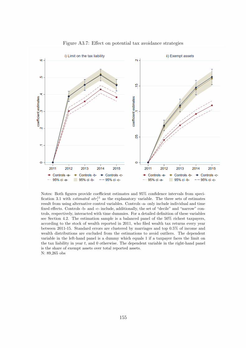
Figure A3.7: Effect on potential tax avoidance strategies
Notes: Both figures provide coefficient estimates and 95% confidence intervals from speci-fication 3.1 with estimated atr11i as the explanatory variable. The three sets of estimatesresult from using alternative control variables. Controls -a- only include individual and timefixed effects. Controls -b- and -c- include, additionally, the set of “decile” and “narrow” con-trols, respectively, interacted with time dummies. For a detailed definition of these variablessee Section 4.2. The estimation sample is a balanced panel of the 50% richest taxpayers,according to the stock of wealth reported in 2011, who filed wealth tax returns every yearbetween 2011-15. Standard errors are clustered by marriages and top 0.5% of income andwealth distributions are excluded from the estimations to avoid outliers. The dependentvariable in the left-hand panel is a dummy which equals 1 if a taxpayer faces the limit onthe tax liability in year t, and 0 otherwise. The dependent variable in the right-hand panelis the share of exempt assets over total reported assets.N: 89,265 obs
155

Figure A3.8: Effect on income and long-term capital gains
Notes: Both figures provide coefficient estimates and 95% confidence intervals from speci-fication 3.1 with estimated atr11i as the explanatory variable. The three sets of estimatesresult from using alternative control variables. Controls -a- only include individual and timefixed effects. Controls -b- and -c- include, additionally, the set of “decile” and “narrow” con-trols, respectively, interacted with time dummies. For a detailed definition of these variablessee Section 4.2. The estimation sample is a balanced panel of the 50% richest taxpayers,according to the stock of wealth reported in 2011, who filed wealth tax returns every yearbetween 2011-15. Standard errors are clustered by marriages and top 0.5% of income andwealth distributions are excluded from the estimations to avoid outliers. The dependentvariable in the left-hand panel is the log of taxable income. The dependent variable in theright-hand panel is the share of long term capital gains over taxable income.N: 69,405 obs
156

Figure A3.9: Effect on real estate
Notes: All figures provide coefficient estimates and 95% confidence intervals from specifica-tion 3.1 with estimated atr11i as the explanatory variable. The three sets of estimates resultfrom using alternative control variables. Controls -a- only include individual and time fixedeffects. Controls -b- and -c- include, additionally, the set of “decile” and “narrow” controls,respectively, interacted with time dummies. For a detailed definition of these variables seeSection 4.2. The estimation sample is a balanced panel of the 50% richest taxpayers, accord-ing to the stock of wealth reported in 2011, who filed wealth tax returns every year between2011-15. Standard errors are clustered by marriages and top 0.5% of income and wealthdistributions are excluded from the estimations to avoid outliers. The dependent variablefor the panels (from left to right) is the share of (all/taxable/exempt) real estate over totalreported assets.N: 89,265 obs
157

Figure A3.10: Effect on unlisted companies and business assets
Notes: All figures provide coefficient estimates and 95% confidence intervals from specifica-tion 3.1 with estimated atr11i as the explanatory variable. The three sets of estimates resultfrom using alternative control variables. Controls -a- only include individual and time fixedeffects. Controls -b- and -c- include, additionally, the set of “decile” and “narrow” controls,respectively, interacted with time dummies. For a detailed definition of these variables seeSection 4.2. The estimation sample is a balanced panel of the 50% richest taxpayers, accord-ing to the stock of wealth reported in 2011, who filed wealth tax returns every year between2011-15. Standard errors are clustered by marriages and top 0.5% of income and wealthdistributions are excluded from the estimations to avoid outliers. The dependent variablefor the panels (from left to right) is the share of (all/taxable/exempt) unlisted companiesand business assets over total reported assets.N: 89,265 obs
158

Figure A3.11: Effect on listed equity and investment funds
Notes: All figures provide coefficient estimates and 95% confidence intervals from specifica-tion 3.1 with estimated atr11i as the explanatory variable. The three sets of estimates resultfrom using alternative control variables. Controls -a- only include individual and time fixedeffects. Controls -b- and -c- include, additionally, the set of “decile” and “narrow” controls,respectively, interacted with time dummies. For a detailed definition of these variables seeSection 4.2. The estimation sample is a balanced panel of the 50% richest taxpayers, ac-cording to the stock of wealth reported in 2011, who filed wealth tax returns every yearbetween 2011-15. Standard errors are clustered by marriages and top 0.5% of income andwealth distributions are excluded from the estimations to avoid outliers. The dependentvariable for the panels (from left to right) is the share of (all/taxable/exempt) listed equityand investment funds over total reported assets.N: 89,265 obs
159

Figure A3.12: Effect on bank accounts and bonds
Notes: The figure provides coefficient estimates and 95% confidence intervals from specifica-tion 3.1 with estimated atr11i as the explanatory variable. The three sets of estimates resultfrom using alternative control variables. Controls -a- only include individual and time fixedeffects. Controls -b- and -c- include, additionally, the set of “decile” and “narrow” controls,respectively, interacted with time dummies. For a detailed definition of these variables seeSection 4.2. The estimation sample is a balanced panel of the 50% richest taxpayers, accord-ing to the stock of wealth reported in 2011, who filed wealth tax returns every year between2011-15. Standard errors are clustered by marriages and top 0.5% of income and wealthdistributions are excluded from the estimations to avoid outliers. The dependent variable isthe share of bank accounts and bonds over total reported assets.N: 89,265 obs
160

Figure A3.13: Effect on gifts
Notes: The figure provides coefficient estimates and 95% confidence intervals from specifica-tion 3.1 with estimated atr11i as the explanatory variable. The three sets of estimates resultfrom using alternative control variables. Controls -a- only include individual and time fixedeffects. Controls -b- and -c- include, additionally, the set of “decile” and “narrow” controls,respectively, interacted with time dummies. For a detailed definition of these variables seeSection 4.2. The estimation sample is a balanced panel of the 50% richest taxpayers, accord-ing to the stock of wealth reported in 2011, who filed wealth tax returns every year between2011-15. Standard errors are clustered by marriages and top 0.5% of income and wealthdistributions are excluded from the estimations to avoid outliers. The dependent variable isa dummy which equals 1 if a taxpayer makes a gift - declared to the Catalan Tax Agency -in year t, and 0 otherwise.N: 89,265 obs
161

162

Chapter 4
Detecting Tax Evasion Through
Wealth Tax Returns
4.1 Introduction
Tax evasion has important and harmful consequences for society; it distorts the
equity and fairness of the tax systems and reduces government budgets, which
in turn translates into less public investment and less social expenditure. The
main challenge tax agencies face in fighting this problem is its undetectability.
The existence of jurisdictions with banking secrecy and low or no taxation
- commonly known as tax havens - extremely complicates the traceability of
evasion practices.
Indeed, wealth held offshore does not seem negligible: Zucman (2013) esti-
mates that the equivalent of 10% of world GDP is held in tax havens, although
there is heterogeneity across countries (Alstadsæter, Johannesen and Zucman,
2018). Alstadsæter, Johannesen and Zucman (2019) show that, in the case of
Scandinavian countries, offshore tax evasion is very concentrated at the top
of the wealth distribution. In particular, authors find that the 0.01% richest
households evade about 25% of their taxes.1 Overall, little is still known about
tax evasion of richest individuals because it can hardly be detected through
random tax audits (Alstadsæter, Johannesen and Zucman, 2019).
In this context, this paper2 exploits a tax amnesty implemented by the
Spanish government in 2012 to study tax evasion among the wealthiest tax-
payers. Using administrative data we are able to identify wealth tax evaders
1This share is far above the 2.8% or the 2.2% income tax gap estimated for Denmarkin Kleven et al. (2011) and Alstadsæter, Johannesen and Zucman (2019), respectively, fromusing different waves of random audits conducted by the Danish Tax Authority.
2This paper is joint work with Daniel Mas Montserrat.
163

and observe the information they were reporting while evading. In particu-
lar, through belated wealth tax returns submitted after the voluntary period
- by the end of the tax amnesty program -, we are able to identify taxpay-
ers voluntarily disclosing previously hidden wealth and quantify the levels of
evasion.
In this regard, the objective of the paper is twofold. First, we want to
describe the evasion voluntarily disclosed. Not only in aggregate terms, but
also across taxpayers’ wealth distribution. As previously anticipated, little is
still known about the levels of evasion among the wealthier and its distribution.
Moreover, little information from the Spanish tax amnesty is publicly available,
thus the findings reported here might be useful to learn more about who, and
to what extent, participated in this voluntary disclosure program. Second,
we want to learn whether tax evaders can be detected with the information
they initially report - i.e. when evasion is still not disclosed -, and if so, how
can they be detected. The answer to this question might have relevant policy
implications since it can be of great use for governments and tax agencies
fighting against tax fraud.
Wealth taxpayers in Catalonia disclosed previously hidden wealth of, at
least, 10,829 million euros, which accounts for 5.4% of the Catalan GDP. The
data indicates that most of the disclosed wealth relates to financial assets,
which necessarily must reflect wealth held abroad (except for cash), since the
Spanish Tax Agency automatically receives information on financial assets held
in Spanish entities.
Taxpayers initially reporting lower levels of wealth are less likely to volun-
tarily disclose evaded wealth, but, in the case they do, the portion disclosed
and the share of taxes evaded is higher, on average. When ranking taxpayers
according to their total wealth (including the portion disclosed), the probabil-
ity of voluntarily disclosing hidden assets increases with wealth, up to almost
45% for the top 1% of wealth taxpayers (which represent around 0.01% of the
population of income tax filers). Wealth disclosers evaded, on average, 30%
of their wealth, regardless of their position in the upper half of the wealth
distribution. Evaders who filed in the voluntary period were initially evad-
ing, on average, 60% of their wealth tax liabilities and between 5 and 30% of
the income taxes owed. The former average stays constant across most of the
distribution, but the latter increases with wealth.
This first part of the paper contributes to the broad literature on tax eva-
sion3, but in particular, to the literature studying offshore evasion (e.g. Roine
3See Slemrod (2018) for a review of recent studies.
164

and Waldenstrom, 2009; Zucman, 2015; Alstadsæter, Johannesen and Zucman,
2018) and, more specifically, to the scarce empirical literature analysing, at in-
dividual level, the participation in tax amnesties and voluntary disclosure pro-
grams (Johannesen et al., 2018; Alstadsæter, Johannesen and Zucman, 2019;
Londono-Velez and Avila-Mahecha, 2019).4
Next, we frame tax evasion detection as a binary classification problem.
Given the values reported in wealth tax returns filed during the voluntary pe-
riod by each taxpayer, we estimate the probability of this being evader with
a binary classifier. We train and evaluate multiple classifiers commonly used
in supervised machine learning methods. Accuracy rates are very similar be-
tween linear and non-linear methods and approximate the upper bound of the
estimated maximum achievable accuracy, which is 68.8%. Therefore, with the
relatively little information available from wealth tax returns, which mostly
relates to wealth composition and income levels, it is already possible to dis-
tinguish evaders from (presumably) non-evaders with an accuracy around 65%.
This second part of the paper contributes to the literature on machine
learning and tax fraud detection. While machine learning, and recently Deep
Learning, are commonly used in solving many problems of computer vision
and natural language processing5, such methods are still less predominant in
economics and other social sciences.6 Nonetheless, they have also been used
in detecting fraudulent activities: unauthorized use of credit card or mobile
transactions (e.g. Adewumi and Akinyelu, 2017; Choi and Lee, 2018), fraud-
ulent insurance claims (e.g. Palacio, 2018), corruption (e.g. Lopez-Iturriaga
and Sanz, 2018) and tax evasion (e.g. Serrano et al., 2012; Castellon Gonzalez
and Velasquez, 2013; Junque de Fortuny et al., 2014; Tian et al., 2016; Shukla
et al., 2018; Perez Lopez, Delgado Rodrıguez and de Lucas Santos, 2019). The
existing literature mainly studies tax evasion detectability in common taxes
such as personal or corporate income taxation or VAT. Hence, this is - to the
best of our knowledge - the first paper trying to predict wealth tax evasion
among the wealthier. We are aware of the limitations of this exercise, which re-
late to a potential self-selection of evaders participating in voluntary disclosure
programs. Nonetheless, given that little is still known about wealth evasion
4Other papers analyse tax amnesties and voluntary disclosure programs from a theoreti-cal perspective or from an aggregate level (Bayer, Oberhofer and Winner, 2015; Langenmayr,2017; Andersson, Schroyen and Torsvik, 2019).
5LeCun, Bengio and Hinton (2015) provide an explanation of different methods andseveral examples.
6For those readers not familiarized with machine learning techniques, Mullainathan andSpiess (2017) provide an insightful illustration of how supervised machine learning methodswork and discuss which kind of economic problems can and cannot be solved by applyingthese methods.
165

and wealthy evaders, we believe it might still be useful to detect this type
of evaders, not only for research purposes, but also to governments and tax
authorities. Moreover, the same exercise could be applied to evaders named in
leaked data such as Swiss leaks or Panama papers (as long as tax authorities
collect enough observable characteristics).
The remaining of the paper proceeds as follows: In section 4.2 we present
the institutional setting regarding the tax amnesty studied. In section 4.3 we
introduce the data employed and discuss evasion categorization. In section 4.4
we quantify the levels of evasion voluntarily disclosed and in section 4.5 we
describe its distribution across taxpayers’ wealth percentiles. In section 4.6 we
present the tax evasion detection exercise and section 4.7 concludes.
4.2 Tax amnesty
At the end of March 2012, the Spanish government passed a law which enabled
to regulate and implement a tax amnesty until November of that year. The
legislation which regulated the particularities of the tax amnesty was passed
on May 317, although two additional reports were issued by the Ministry of
Finance on June 27 and October 11 to clarify several aspects of this measure.
In this regard, the tax amnesty was initially perceived as a 10% tax on evaded
assets and rights held until the end of 2010. Nevertheless, the first report issued
by the Ministry of Finance changed the interpretation of the norm and stated
that the 10% tax should be only applied to the evaded wealth generated dur-
ing the non-prescribed years.8 Thus the tax amnesty offered the possibility to
regularize evaded income by paying a 10% tax on the gross revenues generated
7Orden HAP/1182/2012, de 31 de mayo, por la que se desarrolla la disposicion adi-cional primera del Real Decreto-ley 12/2012, de 30 de marzo, por el que se introducendiversas medidas tributarias y administrativas dirigidas a la reduccion del deficit publico,se aprueban cuantas medidas resultan necesarias para su cumplimiento, ası como el modelo750, declaracion tributaria especial, y se regulan las condiciones generales y procedimientopara su presentacion.
8 Tax prescription period in Spain is four years starting when the voluntary tax filingperiod ends. In the case of tax crimes (i.e. when the owed tax liability exceeds 120,000euros), the prescription period at that time was of five years instead. The voluntary periodto file personal income taxes of calendar year t ends at the very end of June or at thebeginning of July of year t+ 1. Therefore, in the case of natural persons, the non-prescribedyears affected by the tax amnesty were 2007 to 2010 (or 2006 to 2010 for potential taxcriminals willing to avoid criminal charges) if the voluntary disclosure form was submittedbefore July 2012. On the contrary, if the voluntary disclosure form was submitted fromJuly 2012 on, the non-prescribed years were 2008 to 2010 (or 2007 to 2010 for potential taxcriminals). In the case of corporations it depended on the specific fiscal year of the firm.
166

from evaded wealth between 2008 and 2010.9 Moreover, taxpayers partici-
pating in this program would be exempt from fines, interests and fees and
also prevented from tax crime charges. Additionally, the amnesty regulation
ensured further protection to participants with regards to their anonymity -
participants’ identity could not be disclosed - and tax audits procedures, which
could not be initiated with this tax declaration.
Evaders could also legalise their situation through the standard procedure,
which consisted of paying back taxes from the non-prescribed years with an
additional charge up to 20% and a 5% interest rate.10 The personal income
tax rates enforced at that time ranged between 18% (2007-2009) to almost
21% (2010) for financial capital income. The top marginal tax rate for the
remaining types of income was of 43% during the 2007-2010 period, and it was
applicable on taxable bases exceeding around 50,000 euros.
The tax amnesty allowed to regularize evaded income earned until 2010,
thus it was very likely that participants in the program had to amend 2011
income tax returns as well. Moreover, the amnesty only reached income taxes
(either personal, corporate or non-resident income taxes), which in turn im-
plied that its participants needed to legalise their situation with respect to
other taxes such as VAT or the wealth tax. The Spanish government had
reintroduced the net wealth tax in 201111 and hence taxpayers participating
in the amnesty needed to submit an amended 2011 wealth tax return to avoid
being sanctioned (and eventually prosecuted for tax crimes).
The last month of the tax amnesty was accompanied by a tightening of
the tax law and sanctions. On October 29, 2012, the government passed a law
which requires tax residents to report assets held abroad and highly sanctions
those failing to do so.12 In particular, each omitted value carries a 5,000 euros
fine. Moreover, if the Tax Agency discovers these undeclared assets, they will
be considered as unjustified capital gains from the oldest non-prescribed year
and taxed accordingly.13 Besides charges and interests, an additional fine of
9The way to compute the evaded income was not straightforward because of manyspecificities of its regulation; however, it goes beyond the scope of the paper to go deeperinto this matter.
10The interest rate was only enforceable when the emended tax returns were submittedmore than 12 months later than the voluntary period.
11Chapter 3 provides detailed information on the reintroduction of the wealth tax andits regulation.
12Additionally, during the amnesty period it was being processed a change in the criminallaw to harden imprisonment charges for tax crimes and to increase the prescription periodfrom 5 to 10 years. This legislative change was finally passed on December 27, 2012.
13Unjustified capital gains are classified as “general” income instead of financial, andhence they could be taxed up to 43% during the 2008-2010 period.
167
150% of the tax owed will be also imposed.
Overall, very little information has been revealed about the tax amnesty.
On January 2013 the Minister of Finance reported some general facts14: 29,683
taxpayers participated in the amnesty program, being 98% of them natural per-
sons; 93% of the forms were submitted during the last month of the program;
the amnesty collected 1,192 million euros (without considering the indirect
revenues emerging from it) and it legalized around 40,000 million euros of
previously hidden wealth, but 70% of it was related to prescribed years.
Putting these 40,000 million euros in perspective: i) they account for 3.85%
of the Spanish GDP in 2012;15,16 ii) they represent one third of the wealth held
in tax havens by Spaniards in 2007 according to Alstadsæter, Johannesen and
Zucman (2018)17, although comparable shares reduce to about one fifth when
using Spaniards’ undeclared wealth estimates from later years;18 iii) accord-
ing to the information reported by taxpayers to the tax agency as a result of
the new law passed on October 2012, the total wealth held abroad by Span-
ish residents in 2012 amounted to 91,004 million euros, including the assets
voluntarily disclosed in the tax amnesty.19
4.3 Data
This paper uses the universe of anonymized wealth tax returns filed by Cata-
lan taxpayers for the year 2011. These microdata, provided by the Catalan
Tax Agency, contains information on wealth composition and taxable income
14See the press release from the Ministry of Finance on January 23, 2013.15GDP Source: The National Statistics Institute (INE).16As a comparison, the wealth disclosed in the voluntary disclosure program carried out
in Colombia and studied in Londono-Velez and Avila-Mahecha (2019) accounted for 1.73%of GDP.
17This share is higher than the one resulting from offshore wealth disclosed by U.S.households estimated in Johannesen et al. (2018). Authors’ estimations suggest that offshorewealth disclosed in 2009 represented around 10% of the total offshore wealth owned by U.S.households computed in Alstadsæter, Johannesen and Zucman (2018).
18Zucman (2014) estimates an amount of 144,000 million euros of unreported offshorewealth held by Spanish households in 2013. Following a similar methodology than Zucman(2013, 2014), complemented with information on assets held abroad reported to the Span-ish tax authorities, Artola Blanco et al. (2019) estimate that unreported offshore wealthamounted to 158,915 million euros in 2012. Alternatively, Duran-Cabre et al. (2019) esti-mate an amount of 75,062 million euros for 2014 following the methodology proposed byRoine and Waldenstrom (2009). If we express the 40,000 million euros disclosed in 2012 rel-ative to the different estimates of undeclared offshore wealth, including the disclosed wealthin the denominator, we obtain shares of 22%, 20% and 35% respectively.
19Source: Press release from the Ministry of Finance, July 29, 2016 Evolucion del patri-monio neto a partir del ‘modelo 720’.
168

of each taxpayer. In particular, it provides the total stock of reported wealth
classified into real estate and main residence exemption, bank accounts, bonds,
investment funds, business assets, quoted shares and unlisted companies - both
exempt and non-exempt -, life insurance, vehicles, jewellery, artwork, property
rights, debts and “other”, including all taxable wealth not previously catego-
rized. Chapter 3 provides a more detailed description of this database and the
institutional context regarding the wealth tax.
The submission date is also available and this is crucial for our analysis
because it allows us to identify tax returns submitted later than the volun-
tary filing period. Figure 4.1 shows the histogram of 2011 wealth tax returns
by submission date. Each bar comprises one week. We categorize as (for-
mer) evaders those taxpayers filing 2011 wealth tax returns from October 2012
onwards, time when the voluntary period had already expired. We cannot cer-
tainly know whether these taxpayers participated in the tax amnesty, however,
the timing and magnitude of the submissions strongly suggest a relation with
the voluntary disclosure program. As explained in the previous section, the
amnesty only reached income taxes. Consequently, once the voluntary disclo-
sure form was filed, taxpayers needed to amend returns from other taxes, such
as the wealth tax, to avoid being sanctioned or prosecuted for tax crimes.20
Therefore, amnesty participants were very likely to submit 2011 wealth tax
returns during the last two months of 2012.
To further assure that belated 2011 returns are related to the voluntary
disclosure program and not to something recurrent, Figure A4.1 shows the
histogram of wealth tax returns from 2012 to 2015 by submission date. This
Figure allows to verify that filing wealth tax returns months after the end of
the voluntary period was not a usual fact, besides 2011 returns. Contrary to
what happened at the end of 2012, wealth tax returns submitted by the end
of the following years are indeed negligible.21
We cannot distinguish taxpayers directly involved in the tax amnesty from
those who did not participate in the program but, given the hardened laws and
sanctions, decided to disclosure hidden wealth through the standard procedures
described in the previous section. Nonetheless, both types of taxpayers share
the same label - they are evaders - and both situations share the same result:
the voluntary disclosure of evaded wealth, which was the ultimate goal of the
20Official reports from the Ministry of Finance and the Spanish Tax Agency confirmthis was indeed the case. See the Annual Tax Collection Report from 2012 or the pressrelease from September 20, 2016 titled “Efecto del ‘720’ y el ‘750’ en el Impuesto sobre elPatrimonio”.
21Wealth tax returns from 2012 to 2015 submitted in October of the following year, orlater on, represent between 0.10% and 0.17% of all wealth tax returns filed for a given period.
169

enforcement initiatives carried out by the government during that period.
It could be the case that amnesty participants filed the wealth tax return
already incorporating previously hidden wealth during the voluntary period
and, hence, they did not submit amended returns later on. In this situation,
we would be missing to identify some true evaders. However, this is very
unlikely to be the case for several reasons. First, the interpretation of the law
regulating the tax amnesty was very ambiguous until the Ministry of Finance
issued the first clarifying report on June 27, 2012. Given the particularities of
the law and the report, it was difficult to prepare the voluntary disclosure form
and the wealth tax return within 5 days. Second, as explained in footnote 8,
the non-prescribed years affected by the tax amnesty reduced from 2007-2010
to 2008-2010 if the voluntary disclosure form was submitted from July 2012
on, once the voluntary period to file personal income and wealth taxes was
ended. And third, as mentioned in the previous section, 93% of the voluntary
disclosure forms were submitted during November 2012, the last month of the
program.
4.4 Evasion voluntarily disclosed in belated
wealth tax returns
Focusing on those categorised as (former) tax evaders, we observe the following
facts: 6,728 taxpayers filed a 2011 wealth tax return since October 2012. They
represent 15.2% of all wealth taxpayers in Catalonia for the year 2011. This
number of taxpayers also accounts for 22.7% of the overall tax amnesty par-
ticipants in Spain, excluding corporations. Out of the 6,728 taxpayers, 4,474
of them had previously filed a wealth tax return during the voluntary period.
In terms of wealth holdings, these 4,474 evaders account for almost 20% of
the overall stock of wealth reported during the voluntary period (see section
[b.1] of Table 4.1). This share raises up to 26.56% when including the previ-
ously hidden wealth in the numerator (see section [b.2]). Therefore, the evaded
wealth by this group represents 6.73% of the overall wealth holdings reported
during the voluntary period by all taxpayers. More specifically, as shown in
Table 4.1, the total difference in reported wealth holdings between the last and
the former returns of the 4,474 evaders amounts to 8,066 million euros, which
accounts for almost 34% of the wealth initially reported by this group. Put
differently, these taxpayers were hiding 25% of their wealth holdings or more
than half of the assets that should be taxed. Indeed, the last section of panel B
of Table 4.1 also shows that this evaded wealth corresponds to taxable wealth
170

almost entirely.
In this regard, Figure 4.2 provides the asset composition of the 8,066 million
euros previously evaded. In particular, it shows the difference in reported
amounts between the last and former returns for each type of asset, relative
to the total evaded wealth. According to what is reflected in Table 4.1, most
of the evaded wealth is taxable; exempt assets barely change and, if anything,
the reported values decrease. The categories which explain a higher portion
are mainly related to financial assets, taxable unlisted companies and “other”.
Evaded financial assets must reflect wealth held abroad (except for cash), since
the Spanish tax administration automatically receives information on financial
assets held in Spanish financial entities. Evaded unlisted companies could
reflect wealth evaded through shell companies, whereas the “other” category
usually reflects credit rights, among others.22
Panel (a) of Figure A4.2 shows, in the left-axis, the wealth composition of
the evaders filing during the voluntary period, once the former evaded wealth
is declared, and, in the right-axis, it shows the portion previously evaded of
each wealth category. The evaded share of all categories related to taxable
assets ranges around 40% or above - up to almost 80% -, except for unlisted
companies (30%) and real estate (5%). The categories most evaded are bonds
(or similar assets), listed equity and “other” (i.e. the remaining assets not
categorized).
Coming back to panel B of Table 4.1, it also provides information on evaded
income. The taxable income reported by the 4,474 evaders during the volun-
tary period accounts for about 16% of the overall taxable income reported
during that period.23 The total difference in reported taxable income between
the last and the former returns amounts to 254 million euros, which accounts
for 35.57% of the income initially reported by this group. Nevertheless, this
difference should be considered as an upper bound, since around 10% of the
tax evaders did not fill the information on taxable income during the voluntary
period. If we only consider those tax evaders initially reporting information
on income, the total difference reduces to 198 million euros (which should be
considered as a lower bound).
Finally, the panel C of Table 4.1 provides information on the remaining
2,254 evaders who did not submit a 2011 wealth tax return during the voluntary
22Credit rights would emerge, for instance, when accounts that used to be held individ-ually are now co-owned, and the co-owners establish lending agreements between them toavoid being levied by the gift tax.
23This share is imprecise because some taxpayers fail to report information on income(13% of them report zero income), although they might report it correctly in the personalincome tax returns.
171

period; they filed it for the first time on October 2012 or later on. The total
stock of wealth and income reported by this group amounts to 5,446 and 225
million euros, respectively.24 However, it might not be correct to associate
the totality of these amounts to previously hidden wealth. It could be the
case that their taxable wealth held in Spain was lower than the 700,000 euros
taxable threshold and, hence, they opted not to file wealth tax returns during
the voluntary period. Additionally, as seen above, it is very unlikely that
previously hidden wealth comes from exempt assets. Therefore, a (very high)
upper bound of evaded wealth would result from assuming that all reported
wealth was previously hidden, but exempt assets. It amounts to 4,333 million
euros. A lower bound of evaded wealth results from assuming that all reported
wealth below the taxable threshold was already legalized and only the wealth
fully taxed - i.e. exceeding the threshold - was previously hidden. This lower
bound corresponds to 2,763 million euros.
Taking the most conservative value of 2,763 million euros of evaded wealth
by the “initially non-filers”, together with the 8,066 million euros evaded by the
“initial filers”, it translates into a total evaded wealth of 10,829 million euros.
Putting this figure into perspective, it equals to 27% of the 40,000 million
euros legalized by the entire population participating in the tax amnesty all
over Spain. This share is close to the portion of tax amnesty revenues collected
from tax residents in Catalonia relative to Spain’s total25 - i.e. 25.4% -, which
in turn indicates the portion of wealth related to non-prescribed years that
was disclosed by individuals residing in Catalonia.26 Alternatively, the 10,829
million euros disclosed in 2011 wealth tax returns represented 5.4% of the
Catalan GDP in 2011.27
Table 4.2 shows the impact of the disclosure of this previously hidden wealth
in terms of 2011 tax revenues. The extra wealth tax revenues accrued from
October 2012 on amount to 107 million euros (85 from evaders that were
already filing wealth tax returns during the voluntary period and 22 from
initially not filing evaders). Hence, the first type of evaders was evading almost
62% of the wealth taxes owed and the second type was evading the 100%. All
in all, the disclosure of hidden wealth increased 2011 wealth tax revenues by
39%. In the case of income tax revenues, the magnitudes should be taken with
caution given that some taxpayers failed to report information on income and
24Panel (b) of Figure A4.2 shows the wealth composition of this group of evaders.25See https://www.nuevatribuna.es/articulo/economia/madrid-y-cataluna-mas-
beneficiados-amnistia-fiscal/20130909174629096246.html.26This is the case because the amnesty levied a 10% rate, and hence the revenues collected
were proportional to the wealth related to non-prescribed years.27GDP Source: The National Statistics Institute (INE).
172

that (part of) the income reported by the “initially not filing” evaders could
not be evaded. An upper bound of the increase in 2011 income tax revenues
would be 128 million euros (68 from evaders filing in the voluntary period
and 60 from those who did not). The lower bound can be obtained when
considering only those tax evaders initially reporting information on income28
and assuming that the income reported by the “initially not filing” evaders was
fully declared. This lower bound amounts to 52 million euros and accounts for
4% of the total income tax liabilities reported during the voluntary period.
Table 4.3 provides a summary of the evasion ranges discussed in this section.
The only type of evasion that we are able to pinpoint precisely is the wealth tax
evasion. On the contrary, the data employed does not allow us to determine the
exact level of undeclared wealth and income, nor the evaded personal income
taxes.
4.5 The distribution of evasion
Since individuals are required to file wealth tax returns only when they face a
positive tax liability or when their overall gross wealth exceeds 2 million euros,
with the data employed we cannot draw the wealth distribution of the entire
population, but only for wealth tax filers. Considering the taxable threshold
of 700,000 euros and the main residence exemption of 300,000 euros, together
with the fact that real estate is assessed below market prices, wealth tax filers
should be placed at the top of the wealth distribution. Indeed, as explained in
Chapter 3, wealth tax filers in Catalonia accounted for about 1.27% of income
tax filers in 2011. Hence, they represented the - known - richest 1% of income
taxpayers.29
First, we will focus on the 4,474 evaders filing in the voluntary period,
since we can compare their situation in the voluntary period to that resulting
from the latest tax return, after voluntarily disclosing hidden wealth. Later we
will compare these taxpayers filing in the voluntary period to those who were
initially non-filers and submitted wealth tax returns for the first time from
October 2012 onwards.
28Around 90% of the evaders filing during the voluntary period reported information onincome.
29One issue of working with administrative data is that we cannot account for non-filers,thus the true richest 1% of income taxpayers could differ from the known richest 1%. Again,research is needed to learn further about tax evasion among the wealthier.
173

4.5.1 Taxpayers filing in the voluntary period
The distribution of evasion changes depending on how evaders are ranked
along the wealth distribution. Taxpayers’ wealth distribution has been com-
puted according to the total wealth reported during the voluntary period by
all tax filers, both evaders and (presumably) non-evaders. Table A4.1 provides
descriptive statistics of the percentile groups of the initial wealth distribution
used in this section. Once this wealth distribution is defined, evaders can be
ranked according to their initial position, this is, the percentile position they
would take considering the net wealth reported during the voluntary period, or,
alternatively, according to their final position, this is, the percentile position
they would take considering the net wealth reported in the latest tax return,
which includes the formerly evaded wealth. Figures 4.3 to 4.5 presented below
will differentiate between the initial and the final position.
Left panels of Figure 4.3 provide the percentile shares of initially reported
and evaded wealth over the total. Right panels provide the same information
for initially accrued and evaded tax liabilities.30 If evaders are ranked according
to the wealth initially reported, both evaded wealth and tax liabilities are less
concentrated at the top of the distribution than the initial counterparts. The
situation changes when evaders are ranked according to their final reported
wealth. In this case, the distributions get closer and evaded wealth is al-
most exactly distributed across wealth percentiles as initially reported wealth,
except for the 95-99 and 99-100 percentiles, in which the former is less concen-
trated. On the contrary, evaded wealth tax liabilities are more concentrated
at the top of the wealth distribution than those initially accrued.
Figure 4.4 shows the portion of self-disclosed evaders filing in the voluntary
period by wealth percentiles. The probability of voluntarily disclosing assets
increases with wealth, and the slope becomes steeper when evaders are ranked
according to their final reported wealth. Taxpayers placed at the top 5% of
the initial wealth distribution were 40% likely to voluntarily disclose hidden
wealth.
Lastly, Figure 4.5 provides the average share of evaded wealth - panel (a)
- and the average share of evaded wealth tax liabilities - panel (b) - by wealth
percentiles. Evaders initially reporting lower levels of wealth disclosed about
30% of their total wealth. This portion gets lower as initially reported wealth
increases, up to 10% for the last wealth percentile. The percentile averages
30Figure A4.3 provides the same information with respect to income and income taxliabilities. However, the distributions might not be fully accurate given that some taxpayersmisreported information on income.
174
of the evaded share of wealth tax liabilities follow also a descending pattern,
ranging between 80% for the bottom of the distribution to 50% for the highest
percentiles. These trends change when considering evaders’ final position: the
average share of evaded wealth increases with final reported wealth up to 25-
27%. The average share of evaded wealth tax liabilities ranges around 60% for
most of the wealth distribution.
Figure A4.4 provides the same information than Figure 4.5 but with re-
spect to income and income tax liabilities. However, Figure A4.4 only consid-
ers evaders filing in the voluntary period who report accurate information on
income. In this case, the shares of evaded income and evaded income tax liabil-
ities follow a very similar trend since average income tax rates barely changed
after including the formerly evaded income. Although we do not observe tax-
payers’ income composition, the relatively low average tax rates, compared to
tax base levels, especially in the upper part of the wealth distribution, suggest
that an important component is financial capital income (financial capital in-
come was taxed at a 21% flat rate above 6,000 euros, whereas general income
was taxed at progressive tax rates ranging between 24 and 49%). In particu-
lar, the mean of evaders’ final average income tax rates (i.e. including evaded
income) increases progressively from 21% at the bottom of the wealth distribu-
tion to 28% at the top, whereas the mean of final taxable income ranges from
80,000 euros to almost 1 million euros, respectively. For these levels of taxable
income, average tax rates would range between 32% and 47% if tax bases were
fully taxed as general income. Thus, real average tax rates are far below these
thresholds. Similar to Figure 4.5, when evaders are ranked according to their
final position, the average share of evaded income and evaded tax liabilities
increase with wealth, from around 4% at the bottom of the distribution to
about 33% at the top 1%.
4.5.2 All evaders voluntarily disclosing wealth
This section will compare the evasion disclosed by taxpayers who filed in the
voluntary period with that disclosed by taxpayers filing for the first time in
October 2012 onwards. Since we cannot observe the initial position of evaders
not filing in the voluntary period, we will rank all evaders according to their
final position (i.e. considering the wealth reported in the latest tax return).
Likewise, to get a wealth distribution that considers all taxpayers, even those
not filing in the voluntary period, it needs to be computed according to the
wealth reported in the latest return submitted by each taxpayer, and hence
it will account for previously hidden wealth. Table A4.2 provides descriptive
175

statistics of the percentile groups of this final wealth distribution. The Figures
presented in this section are constructed using this final distribution, although
Figures A4.5 to A4.7 show that things do not substantially change if taxpayer’s
initial wealth distribution (computed in the previous section) is used instead.
As detailed in section 4.4, we cannot determine the exact amount of pre-
viously hidden wealth for evaders not filing in the voluntary period. Hence,
we will consider its lower bound, which corresponds to the portion of wealth
exceeding the taxable threshold.
Figure 4.6 provides the percentile shares of evaded wealth and evaded
wealth tax liabilities over the total and shows that evasion is more concen-
trated among evaders filing in the voluntary period.
Figure 4.7 shows the portion of the two groups of evaders by wealth per-
centiles. One could expect “initially not filing” evaders to be placed at the
bottom of the distribution, but the Figure shows they are quite uniformly dis-
tributed. Around 5% of wealth taxpayers were not filing wealth tax returns
when they had to, regardless of their position in the wealth distribution, ex-
cept for the highest percentile, where the portion lowers to 2%. If considering
all 2011 wealth tax filers, regardless of their submission date, those placed
in the richest percentile (which account for approximately 0.01% of income
tax filers) are 45% likely to voluntarily disclose hidden wealth and, hence, to
evade taxes. This share is close to the 40% rate reported in Londono-Velez
and Avila-Mahecha (2019) and much higher than the 14% rate provided in
Alstadsæter, Johannesen and Zucman (2019).
Figure 4.8 provides the average share of evaded wealth by wealth per-
centiles.31 As already seen in the previous section, the share of evaded wealth
increases with wealth. Compared to evaders filing in the voluntary period,
those who initially did not file wealth tax returns evaded, on average, a con-
siderably higher portion of wealth.32 When considering all evaders voluntarily
disclosing wealth, the average share of evaded wealth ranges around 30% for
the top 60% of the distribution. Strikingly, the share of evaded wealth is the
same for disclosers in Scandinavian countries (see Alstadsæter, Johannesen
and Zucman, 2019) or in Colombia (see Londono-Velez and Avila-Mahecha,
2019).
31Figure A4.8 provides the same information with respect to the share of evaded wealthtax liabilities, although it does not add new relevant information to what has already beendiscussed in Section 4.5.1, since the evaded share of evaders not filing in the voluntary periodis 1.
32Note that in the case of evaders not filing in the voluntary period, the average share ofevaded wealth is computed using the lower bound of previously hidden wealth. Hence, theaverage would be even higher if the upper bound was considered instead.
176

4.6 Tax evasion detection
4.6.1 Methodology
As previously stated, we are interested in studying whether tax evaders can
be detected with the information they initially report (thus evasion is still
not disclosed at that time). Hence, for the exercise of tax evasion detection
developed in this section, we will use the information initially reported in
the wealth tax returns filed during the voluntary period, both for those 4,474
taxpayers categorized as tax evaders and those who - presumably - are not.
The information reported in wealth tax returns provides 34 predictors per
taxpayer, which are mostly related to wealth composition, taxable income and
wealth and income tax liabilities.
Figures 4.9 to 4.11 show the initial wealth composition of different taxpayer
types. In particular, the Figures show the average share of financial assets and
unlisted companies (Figure 4.9), the share of real estate, “unproductive” and
“other” assets (Figure 4.10) and the share of debts (Figure 4.11), by evaders
status (evaders vs. non-evaders) and wealth percentiles groups (0-50, 50-95
and 95-100). According to these Figures, wealth reported by evaders during
the voluntary period had a different composition than wealth reported by
(presumably) non-evaders. Evaders reported a lower share of bank accounts,
life insurances and debts, regardless of the percentile group. On the contrary,
evaders reported a higher portion of unlisted companies (both taxable and
exempt) and vehicles, jewellery and artwork, although the weight of these
last assets is very small (they account for less than 0.3% of reported wealth).
Evaders from percentiles 0-95 also reported a higher share of investment funds
and listed equity and a lower share of real estate. In addition to the common
differences, evaders from the highest 5 percentiles reported a lower share of
bonds and similar assets, investment funds and “other” assets.
In the remaining of the section, we will evaluate how useful these differ-
ences are to detect tax evasion. Since we only observe evaders who voluntarily
disclosed previously hidden wealth, we might not be able to detect all types of
wealth evaders, but only those willing to participate in this type of programs.
The methods implemented in this study would allow to detect wealth evaders
not willing to participate in voluntary disclosure programs if they shared rel-
evant and observable characteristics with those evaders participating in these
programs. Alstadsæter, Johannesen and Zucman (2019) show that, in the case
of Scandinavian countries, self-selection into amnesty programs is negatively
correlated with wealth compared to offshore leaked data, although it is quan-
177

titatively small. However, a further comparison of individuals named in off-
shore leaks with amnesty participants would be needed to determine whether
the later type of evaders is self-selected in terms of asset portfolio or other
characteristics observable in wealth tax returns. Nonetheless, even in the case
that the values reported in wealth tax returns only help to detect evaders who
would potentially participate in a tax amnesty, this is still helpful to tax au-
thorities and governments, since it would dissipate the need to implement this
type of programs, which are unfair to tax compliers and politically costly.
Tax evasion detection as a binary classification problem
Tax evasion detection can be framed as a binary classification problem. In
order to estimate the probability of a given individual, x, being evader, we use
a binary classifier f(x). The classifier assigns a probability of being evader p to
each individual x. According to this estimated probability p, an individual is
predicted to be an evader if p > 50%. Alternatively, an individual is predicted
as a non-evader if p < 50%.
We try several binary classifiers commonly used in supervised machine
learning methods that range over different interpretability and flexibility: Lo-
gistic Regression, Support Vector Machine (SVM) with linear and Radial Basis
Function (RBF) kernels, k-Nearest Neighbour (k-NN), Random Forest (RF),
and a Multi-Layer Perceptron (MLP). Appendix 4.10.2 provides a brief descrip-
tion of each. While classifiers such as logistic regression or linear SVM can be
interpreted by examining their weights, they might lack enough flexibility to
capture non-linear behaviours. On the other hand, methods such as non-linear
SVMs and neural networks can capture complex non-linear behaviours but can
be difficult to interpret.
If trained properly, the accuracy difference between linear models (Logistic
regression and linear SVM) and non-linear models (MLP and RBF SVM) can
provide some insight into the nature of the data. For example, if linear models
perform much better than non-linear methods, we might be overfitting the
non-linear methods. On the contrary, if non-linear methods are performing
much better than the linear ones, we might be facing data that is complex and
non-linear. When both approaches provide similar accuracies, we might have
data that has a linear behaviour and, therefore, complex non-linear methods
are not needed.
We implement the tax evasion detection exercise as follows: first, we ex-
press each predictor relative to total wealth and we normalize it to have zero
mean and unit variance. Then, we randomly discard some non-evader individ-
178
uals to have the same number of observations for each category. This results in
a dataset of 8,948 observations. We then randomly divide this dataset in train-
ing, validation and testing sets including 5,726, 1,432 and 1,790 individuals,
respectively. Finally, we train the binary classifiers.
The training set is used to fit the parameters of each method.33 The valida-
tion set is used to find the best configuration of the classifier. More specifically,
each classifier has different possible configurations (hyperparameters) that de-
fine the size and complexity of the method.34 So first, a wide range of classifiers
with different hyperparameters are learned using the training set. Then, each
of these classifiers is evaluated with the validation set, and the classifiers with
the hyperparameters that obtain higher accuracy are selected (e.g. if a k-NN
classifier with K = 3 has higher accuracy than a k-NN with K = 10, the
former is used). After the best method configuration is chosen, the classifier is
evaluated with the testing set in order to obtain an accuracy value that reflects
the performance when new observations are presented.
In this regard, the training, validation and testing set splits are used in
order to obtain models that will perform properly with new observations. If
only a unique set is used for fitting and evaluating the method, it is very likely
that the classifier will perform successfully with the already seen observations,
but will fail when previously unseen observations are presented.
As shown in Figure 4.4, the portion of self-disclosed evaders increases with
wealth, especially in the highest percentiles. To ensure that wealth is not
driving the entire classification problem, we express the predictors relative
to wealth, as we explained above, and we also implement the tax evasion
detection exercise just described for the bottom 50% of the taxpayers’ wealth
distribution.
Estimation of the expected maximum accuracy
Given that the data employed in this paper has not been used for evasion
detection purposes before, we need to learn how useful is the information
reported in the tax returns to classify an individual as evader or non-evader.
In particular, an estimate of the maximum accuracy that could be achieved
with the given predictors would help us to evaluate the performance of the
classifiers employed. This indicator can be obtained by estimating the Bayes
33In the case of Logistic Regression, SVM and MLP, these parameters include weightsand bias. In the case of a Random Forest, these parameters include the values of the leavesof the trees.
34The hyperparameters include regularization constants for SVMs, number and size ofhidden layers in MLP, number and size of trees in RF and K in k-NN.
179

Error Rate (BER).
The BER gives a lower bound on the error achievable for a classification
problem acting on a given feature or predictor space. The BER is non-zero
when the classification labels are not deterministic (a given set of predictors has
a non-zero probability of belonging to more than one class). In other words,
if the BER is non-zero, that means that two individuals could be described
with identical predictors and each of them belong to different categories. For
example, a BER of 0.5 in a binary classification indicates that no classifier will
surpass random chance accuracy, while a BER of 0 indicates that a powerful
enough classifier could obtain a 100% classification accuracy. Hence, the BER
can be used to estimate the maximum obtainable classification accuracy.
In order to compute the BER, the probability distribution of an individual
belonging to each category given its predictors is needed. Such probability
distribution is rarely known, therefore the BER needs to be approximated.
In perceptual tasks such as image classification, human error can be used as
a proxy for the BER (typically assumed to be negligible). However, in non-
perceptual tasks like tax evasion detection, statistical estimators of the BER
need to be used. Appendix 4.10.3 describes how the bounds of the BER can
be estimated.
The bounds of the BER, Pe(f1, f2), can be used to estimate the bounds of
the expected maximum accuracy Acc as: Acc = 1− Pe(f1, f2).
In the following section we present the estimated bounds on the Acc for
our tax evasion detection problem.
4.6.2 Results
Table 4.4 (top) presents the accuracy rate for each classifier in validation and
testing sets.35 Table 4.4 (bottom) shows the bounds of the estimated max-
imum achievable accuracy. Accuracy bounds higher than 50% indicate that
the data contains some information that can help to detect tax evaders. The
predictors with slightly better performance are MLP and RF, with an accu-
racy rate of almost 69% and about 65.5% in the validation and testing sets,
respectively. Nevertheless, linear and non-linear classifiers have similar accu-
racy rates, which lie within the bounds of the estimated maximum accuracy.
Therefore, the performance of the detection methods employed is close to the
estimated maximum achievable with the information available. In order to in-
crease the accuracy of the classifiers, additional taxpayers’ information should
35Because using the totality of the data instead of using a balanced subset does notprovide a significant change of accuracy, we will only report results with the balanced subset.
180

be needed.
As a robustness check, Table 4.5 presents the accuracy rate obtained with
each classifier in validation and testing sets when implementing the tax eva-
sion detection exercise for the bottom 50% of taxpayers’ wealth distribution.
Accuracy rates are very similar to those presented in Table 4.4.
As an illustration, Figure 4.12 shows two histograms of the estimated prob-
ability of being evader p for each group of taxpayers.36 The blue distribution
relates to those taxpayers categorized as non-evaders and the orange distribu-
tion relates to those categorized as evaders. Panel (a) shows the histograms
of the two groups for the testing set of 1,790 individuals. Panel (b) considers
all taxpayers who filed wealth tax returns during the voluntary period. The
top (bottom) of the estimated probability distribution reflects those evaders
(non-evaders) better predicted by the classifier. Interestingly, the non-evaders
distribution (blue) also presents a peak at high levels of p. Hence, it reflects
those taxpayers initially classified as non-evaders who have an estimated prob-
ability of being evader around 70%.
In this regard, Table 4.6 summarizes the number of taxpayers categorized
as non-evaders whose p exceeds 50%, 60%, 70% and 80%, according to each
classifier employed in this paper. The number of taxpayers with an estimated
probability of being evader higher than 70% ranges between 1,758 and 4,004,
depending on the method employed. These numbers represent between 4.7%
and 10.7% of all taxpayers categorized as non-evaders (i.e. 37,402). These
intervals lower to 141 (0.4%) and 1,145 (3%) when considering those taxpayers
with an estimated probability above 80%. Nonetheless, the involvement of the
tax administration would be required to assess the validity of these predictions.
4.7 Conclusions
In the context of a tax amnesty carried out by the Spanish government in
2012, this paper quantifies the wealth voluntarily disclosed and shows how this
type of evasion was distributed across wealth levels. In line with findings from
other countries, the data indicates that the probability of voluntarily disclosing
hidden assets increases significantly with wealth and that, on average, wealth
disclosers were evading around 30% of their net worth.
The existence of these levels of evasion harms the fairness of the tax systems
and undermines the redistributive role of income and wealth taxation.
36In this case, p is estimated with the classifier Support Vector Machine (SVM) with Ra-dial Basis Function (RBF), but these distributions can be obtained for each other classifier.
181

As a way of fighting this problem, this paper also shows that machine
learning methods can be useful tools for governments and tax administrations
to detect tax evasion. In particular, we study whether wealth evaders can
be detected with the information they initially report in wealth tax returns.
We frame tax evasion detection as a binary classification problem and train
and evaluate multiple classifiers commonly used in supervised machine learn-
ing methods. The main conclusion from this exercise is that the relatively
little information available from tax returns, which mostly relates to wealth
composition and income levels, it already allows distinguishing evaders from
(presumably) non-evaders. Nonetheless, we hypothesize that acquiring more
information from taxpayers, and hence providing a richer description of their
personal, professional and financial profiles might lead to better detectability.
Indeed, a large amount of taxpayers’ information is already available to
public institutions, so an intensive use of it, together with its release for re-
search purposes, might improve fraud detection methods. This has been, in
fact, the path adopted by some tax administrations such as the IRS in the
US, which has been implementing big data analytics programmes since years
ago.37
37https://www.irs.gov/about-irs/strategic-goals/advance-data-analytics
182

4.8 Tables
Table 4.1: 2011 wealth and income reported by different groups of taxpayers
All wealthTaxable wealth
Exemptwealth
TaxableincomeFully taxed
Below thethreshold
A: All taxpayers filing in the voluntary period
[a] Total reported during119,817 40,508 28,527 50,782 4,550
the voluntary period (in eM)% All wealth 33.81 23.81 42.38
B: Evaders filing in the voluntary period
[b.1] Total reported during23,763 7,097 3,045 13,621 713
the voluntary period (in eM)% All wealth 29.87 12.81 57.32
% wrt [a] 19.83 17.52 10.67 26.82 15.68
[b.2] Total reported since31,829 15,117 3,127 13,585 967
October 2012 (in eM)% All wealth 47.49 9.82 42.68
% wrt [a] 26.56 37.32 10.96 26.75 21.25
[b.2]-[b.1] Difference (in eM) 8,066 8,020 82 -36 254% All wealth 99.43 1.02 -0.44
% wrt [b.1] 33.95 113.01 2.69 -0.26 35.57% wrt [b.2] 25.34 53.05 2.62 -0.26 26.24
C: Evaders not filing in the voluntary period
[c] Total reported since5,446 2,763 1,570 1,113 225
October 2012 (in eM)% All wealth 50.73 28.84 20.43
% wrt [a] 4.55 6.82 5.51 2.19 4.95
Notes: The table provides information on 2011 total wealth and taxable income reportedby different groups of taxpayers. In the case of wealth, it distinguishes between all wealthand wealth considered as taxable/exempt by the Wealth Tax Law. Among the wealthconsidered as taxable, only the amount exceeding the taxable threshold of 700,000 eurosis fully taxed ; the amount below the threshold is not levied by the wealth tax. 41,876taxpayers filed a wealth tax return during the voluntary period. 4,474 (2,254) taxpayersbelong to the group of evaders (not) filing a wealth tax return in the voluntary period.
183

Table 4.2: Accrued 2011 revenues by different groups of taxpayers
(1) (2) (3)Accrued tax liabilities: In voluntary period since October 2012 (2)-(1) DifferenceAll taxpayers filing in the voluntary period
Wealth tax (in eM) 274 - -Income tax (in eM) 1,272 - -
Evaders filing in the voluntary period
Wealth tax (in eM) 53 138 85% All wealth tax revenues accrued
19.28 50.39 31.12in the voluntary period
Income tax (in eM) 211 279 68% All income tax liabilities reported
16.55 21.93 5.38in the voluntary period
Evaders not filing in the voluntary period
Wealth tax (in eM) - 22 -% All wealth tax revenues accrued
8.08in the voluntary period
Income tax (in eM) - 60 -% All income tax liabilities reported
4.68in the voluntary period
Notes: 41,876 taxpayers filed a wealth tax return during the voluntary period. 4,474 (2,254)taxpayers belong to the group of evaders (not) filing a wealth tax return in the voluntaryperiod.
184

Table 4.3: Summary of evasion ranges
Lower bound Upper bound
Evaded wealth (in eM) 10,829 12,400% All wealth 8.12 9.30
Evaded wealth tax (in eM) 107 107% All wealth tax revenues 28.16 28.16
Evaded income (in eM) 198 479% All income 3.93 9.52
Evaded personal income tax (in eM) 52 128% All income tax liabilities 3.74 9.14
Notes: All wealth (income) refers to the sum of total wealth (income) lastly re-ported by each taxpayer in 2011 wealth tax returns, including evaded wealth (in-come). All wealth tax revenues refers to the total wealth tax revenues accrued in2011. All income tax liabilities considers the latest income tax liabilities reportedby each taxpayer in the 2011 wealth tax returns.
185

Table 4.4: Accuracy of binary classifiers and accuracy bound estimations
Method Validation Accuracy Testing AccuracyLogistic Regression 66.0% 64.6%Linear SVM 65.3% 63.8%RBF SVM 66.9% 64.7%k-NN 64.3% 62.4%MLP 68.7% 65.4%RF 67.4% 65.5%1− Pe(f1, f2) Lower Bound 57.1%1− Pe(f1, f2) Upper Bound 68.8%
Table 4.5: Accuracy of binary classifiers with 50% lower wealth
Method Validation Accuracy Testing AccuracyLogistic Regression 61.4% 64.5%Linear SVM 60.5% 61.2%RBF SVM 63.7% 66.3%k-NN 61.8% 64.0%MLP 64.5% 65.8%RF 64.1% 63.6%
186

Table 4.6: Summary of taxpayers categorized as non-evaders
whose estimated probability of being evader exceeds 50%
Method p > 50% p > 60% p > 70% p > 80%
Logistic Regression 12,095 6,452 2,081 384SVM (Linear) 11,429 6,792 2,513 284SVM (RBF) 12,142 8,608 4,004 141k-NN 11,998 5,163 1,758 300MLP 13,662 8,000 3,555 1,145RF 12,100 6,525 2,651 447
Notes: This table summarizes the number of taxpayers categorized asnon-evaders whose estimated probability of being evader p exceeds 50%,60%, 70% and 80%, according to each classifier employed. The totalnumber of taxpayers categorized as non-evaders is 37,402.
187

4.9 Figures
Figure 4.1: Histogram of 2011 wealth tax returns by submission week
Notes: Each bar comprises one week. The red vertical line is placed at the end of thevoluntary filing period (July 2), whereas the green vertical line is placed at the end of thetax amnesty program (November 30).
188

Figure 4.2: Asset composition of evaded wealth
Notes: This figure compares, for each category, the total amounts reported since October2012 with those reported in the voluntary period by the 4,474 tax evaders who were filingwealth tax returns in both periods. Each category difference is expressed in terms of thetotal wealth difference (eM 8,066). The two categories of Unlisted companies also includebusiness assets. The positive sign of Debts indicates an increase in the reported amounts,and hence it has a negative impact on total wealth.
189

Figure 4.3: Distribution of reported and evaded wealth and tax liabilities
(a) Evaders’ initial position
(b) Evaders’ final position
Notes: Each distribution of each graph shows the percentile shares over the total. Wealth percentilesare defined according to taxpayers’ initial wealth distribution, this is, according to the total wealthreported during the voluntary period. The distributions plotted in each graph are computed consid-ering only the 4,474 evaders who filed during the voluntary period. Evaders’ initial position reflectsthe percentile position they would take according to the wealth reported during the voluntary pe-riod. Evaders’ final position reflects the percentile position they would take according to the wealthreported in the latest tax return, once the formerly evaded wealth is included.
190

Figure 4.4: Portion of self-disclosed evaders filing in the voluntary period
by wealth percentiles
Notes: The figure shows the portion of self-disclosed evaders among all taxpayers filingduring the voluntary period by wealth percentiles. Wealth percentiles are defined accordingto taxpayers’ initial wealth distribution, this is, according to the total wealth reported duringthe voluntary period. Evaders’ initial position reflects the percentile position they wouldtake according to the wealth reported during the voluntary period. Evaders’ final positionreflects the percentile position they would take according to the wealth reported in the latesttax return, once the formerly evaded wealth is included.
191

Figure 4.5: Percentile averages of evaded wealth and tax liabilities
voluntarily disclosed by evaders filing in the voluntary period
(a) Share of evaded wealth
(b) Share of evaded wealth tax liabilities
Notes: The figure provides, by wealth percentiles, the average share of evaded wealth -Panel (a) - and the average share of evaded wealth tax liabilities - Panel (b) - with their95% confidence intervals. The plotted averages only consider the 4,474 evaders who filedwealth tax returns during the voluntary period. The individual share of evaded wealth andevaded wealth tax liability is computed over taxpayer’s total, including the evaded partin the denominator. Wealth percentiles are defined according to taxpayers’ initial wealthdistribution, this is, according to the total wealth reported during the voluntary period.Evaders’ initial position reflects the percentile position they would take according to thewealth reported during the voluntary period. Evaders’ final position reflects the percentileposition they would take according to the wealth reported in the latest tax return, once theformerly evaded wealth is included.
192

Figure 4.6: Distribution of evaded wealth and tax liabilities;
Filers vs. non-filers in the voluntary period
Notes: Each distribution of each graph shows the percentile shares over the group’s total.4,474 (2,254) taxpayers belong to the group of evaders (not) filing a wealth tax return inthe voluntary period. In the case of evaders not filing in the voluntary period, the evadedwealth is computed as the portion exceeding the taxable threshold of 700,000 euros, whichmight be a lower bound. Wealth percentiles are defined according to taxpayers’ final wealthdistribution, this is, considering the voluntarily disclosed wealth reported in the latest taxreturns, together with that wealth already reported in the voluntary period.
193

Figure 4.7: Portion of self-disclosed evaders by wealth percentiles
Notes: The figure shows the portion of (initially filing/initially not filing/all) evaders amongall wealth taxpayers by wealth percentiles. Wealth percentiles are defined according totaxpayers’ final wealth distribution, this is, considering the voluntarily disclosed wealthreported in the latest tax returns, together with that wealth already reported in the voluntaryperiod.
194

Figure 4.8: Percentile averages of the share of evaded wealth;
Evaders filing vs. not filing in the voluntary period
Notes: The figure provides, by wealth percentiles, the average share of evaded wealth with its95% confidence intervals. The individual share of evaded wealth is computed over taxpayer’stotal, including the evaded part in the denominator. In the case of evaders not filing inthe voluntary period, the evaded wealth is computed as the portion exceeding the taxablethreshold of 700,000 euros, which might be a lower bound. Wealth percentiles are definedaccording to taxpayers’ final wealth distribution, this is, considering the voluntarily disclosedwealth reported in the latest tax returns, together with that wealth already reported in thevoluntary period.
195

Figure 4.9: Initial wealth composition. Financial assets and unlisted companies
196

Figure 4.10: Initial wealth composition. Real estate, ‘unproductive’ assets and other
Figure 4.11: Initial wealth composition. Debts
Notes for Figures 4.9, 4.10 and 4.11: The Figures provide the average initial wealth composition bydifferent taxpayer groups and 95% confidence intervals. This information is provided by percentilesgroups (0-50, 50-95 and 95-100) and distinguishing between (presumably) non-evaders and (self-disclosed) evaders. Each asset (debt) share is computed over total wealth, considering the amountsreported during the voluntary filing period.
197

Figure 4.12: Histograms of the estimated probability of being evader
(a) Testing set
(b) All
Notes: The Figures from panel (a) and panel (b) show the histogram of the estimatedprobability of being evader (in the x axis) for those categorized as non-evaders (in blue)and for those categorized as evaders (in orange). Panel (a) considers the testing set of 1,790observations. Panel (b) considers all the 41,876 wealth taxpayers who filed in the voluntaryperiod. The binary classifier employed to estimate the probabilities presented here is theSupport Vector Machine (SVM) with Radial Basis Function (RBF).
198

4.10 Appendix
4.10.1 Figures and tables
Figure A4.1: Histogram of 2012-2015 wealth tax returns by submission week
Notes: Each bar comprises one week. The red vertical lines are placed at the end of thecorresponding voluntary filing period.
199

Figure A4.2: Evaders’ wealth composition
(a) Evaders filing in the voluntary period
(b) Evaders not filing in the voluntary period
Notes: (1) Bank accounts, (2) Bonds, (3) Investment funds, (4) Listed equity -taxable-,(5) Listed equity -exempt-, (6) Life insurances, (7) Unlisted companies and business assets-taxable-, (8) Unlisted companies and business assets -exempt-, (9) Real Estate, (10) Mainresidence exemption, (11) Vehicles, jewellery, artwork, etc., (12) Other, (13) Debts. Eachbar shows, in the left-axis, the weight of that category over total wealth, according to theamounts reported in the latest 2011 wealth tax returns (which already include formerlyhidden wealth). The share of (13) Debts is expressed in absolute values and has a negativeimpact on total wealth. Dots of Panel (a) indicate, in the right-axis, the (formerly) evadedportion of each category.
200

Figure A4.3: Distribution of reported and evaded income and tax liabilities
(a) Evaders’ initial position
(b) Evaders’ final position
Notes: Each distribution of each graph shows the percentile shares over the total. Wealth percentilesare defined according to taxpayers’ initial wealth distribution, this is, according to the total wealthreported during the voluntary period. The distributions plotted in each graph are computed consid-ering only 3,800 evaders who filed during the voluntary period and seem to report information onincome accurately. Evaders’ initial position reflects the percentile position they would take accordingto the wealth reported during the voluntary period. Evaders’ final position reflects the percentileposition they would take according to the wealth reported in the latest tax return, once the formerlyevaded wealth is included.
201

Figure A4.4: Percentile averages of evaded income and tax liabilities
voluntarily disclosed by evaders filing in the voluntary period
(a) Share of evaded income
(b) Share of evaded income tax liabilities
Notes: The figure provides, by wealth percentiles, the average share of evaded income -Panel (a) - and the average share of evaded income tax liabilities - Panel (b) - with their95% confidence intervals. The plotted averages only consider 3,800 evaders who filed duringthe voluntary period and seem to report information on income accurately. The individualshare of evaded income and evaded income tax liability is computed over taxpayer’s total,including the evaded part in the denominator. Wealth percentiles are defined according totaxpayers’ initial wealth distribution, this is, according to the total wealth reported duringthe voluntary period. Evaders’ initial position reflects the percentile position they wouldtake according to the wealth reported during the voluntary period. Evaders’ final positionreflects the percentile position they would take according to the wealth reported in the latesttax return, once the formerly evaded wealth is included.
202

Figure A4.5: Distribution of evaded wealth and tax liabilities;
Initial vs. final wealth distribution
Notes: Each distribution of each graph shows the percentile shares over the total. The twodistributions plotted in each graph are computed considering only the 4,474 evaders who filedduring the voluntary period. The difference between the two comes from whether evadersare placed according to the initial or the final wealth distribution (x-axis). In both cases,the evaders’ percentile assignment is made according to the wealth reported in their latesttax returns (i.e. final position). The Initial wealth distribution is defined according to thetotal wealth reported during the voluntary period. The Final wealth distribution is definedconsidering the voluntarily disclosed wealth reported in the latest tax returns, together withthat wealth already reported in the voluntary period.
203

Figure A4.6: Portion of self-disclosed evaders filing in the voluntary period;
Initial vs. final wealth distribution
Notes: The figure shows the portion of self-disclosed evaders among all taxpayers filingduring the voluntary period by wealth percentiles. The difference between the two plottedlines comes from whether evaders are placed according to the initial or the final wealthdistribution (x-axis). In both cases, the evaders’ percentile assignment is made accordingto the wealth reported in their latest tax returns (i.e. final position). The Initial wealthdistribution is defined according to the total wealth reported during the voluntary period.The Final wealth distribution is defined considering the voluntarily disclosed wealth reportedin the latest tax returns, together with that wealth already reported in the voluntary period.
204

Figure A4.7: Percentile averages of evaded wealth and tax liabilities
voluntarily disclosed by evaders filing in the voluntary period;Initial vs. final wealth distribution
(a) Share of evaded wealth
(b) Share of evaded wealth tax liabilities
Notes: The figure provides, by wealth percentiles, the average share of evaded wealth -Panel (a) - and the average share of evaded wealth tax liabilities - Panel (b) - with their95% confidence intervals. The two averages plotted in each graph are computed consideringonly the 4,474 evaders who filed during the voluntary period. The difference between thetwo comes from whether evaders are placed according to the initial or the final wealthdistribution (x-axis). In both cases, the evaders’ percentile assignment is made accordingto the wealth reported in their latest tax returns (i.e. final position). The Initial wealthdistribution is defined according to the total wealth reported during the voluntary period.The Final wealth distribution is defined considering the voluntarily disclosed wealth reportedin the latest tax returns, together with that wealth already reported in the voluntary period.
205

Figure A4.8: Percentile averages of the share of evaded tax liabilities;
Evaders filing vs. not filing in the voluntary period
Notes: The figure provides, by wealth percentiles, the average share of evaded wealth taxliabilities with its 95% confidence intervals. The individual share of evaded wealth taxliability is computed over taxpayer’s total, including the evaded part in the denominator.Wealth percentiles are defined according to taxpayers’ final wealth distribution, this is,considering the voluntarily disclosed wealth reported in the latest tax returns, together withthat wealth already reported in the voluntary period.
206

Table A4.1: Taxpayers’ initial wealth distribution
Percentiles Obs Mean Std. Dev. Min Max
0-10 4,188 793,634 393,298 -21,000,000 876,55010-20 4,188 935,164 33,232 876,579 993,41920-30 4,186 1,053,554 34,847 993,471 1,113,62230-40 4,188 1,185,599 43,458 1,113,632 1,263,64640-50 4,188 1,354,224 55,633 1,263,847 1,455,34150-60 4,188 1,583,424 78,704 1,455,369 1,731,76560-70 4,187 1,943,477 130,890 1,731,853 2,184,47970-80 4,187 2,527,261 223,388 2,184,525 2,957,77280-90 4,188 3,745,262 549,875 2,957,899 4,908,94190-95 2,094 6,209,951 865,561 4,909,163 7,993,31995-99 1,676 12,612,187 3,967,261 8,003,489 23,552,31499-100 418 53,475,493 51,836,413 23,577,301 436,577,889
Table A4.2: Taxpayers’ final wealth distribution
Percentiles Obs Mean Std. Dev. Min Max
0-10 4,413 797,065 383,559 -21,000,000 882,14110-20 4,413 942,486 34,543 882,154 1,003,05020-30 4,413 1,065,564 36,189 1,003,056 1,129,05930-40 4,413 1,204,295 45,726 1,129,063 1,286,11640-50 4,413 1,383,357 59,270 1,286,136 1,492,91250-60 4,413 1,631,045 86,423 1,492,953 1,794,65560-70 4,413 2,017,887 136,701 1,794,740 2,273,03770-80 4,413 2,643,875 238,473 2,273,109 3,107,27480-90 4,413 3,986,656 612,843 3,107,347 5,313,97990-95 2,207 6,728,028 972,538 5,315,929 8,760,93595-99 1,764 13,773,217 4,364,665 8,761,278 25,878,25399-100 442 56,613,970 54,454,528 25,879,222 436,577,889
Notes for Tables A4.1 and A4.2: According to the Wealth Tax Law, individuals must submit
wealth tax returns when their overall gross wealth exceeds 2 million euros, although their
taxable wealth is below the minimum threshold and hence their tax liability is zero. This
is the reason why the first percentile group includes negative wealth. In fact, 13 tax filers
report negative wealth and 35 tax filers (in Table A4.1) and 32 (in Table A4.2) report taxable
wealth below the taxable threshold of 700,000 euros. Taxpayers’ initial wealth distribution
is defined according to the total wealth reported during the voluntary period. Taxpayers’
final wealth distribution is defined considering the voluntarily disclosed wealth reported in
the latest tax returns, together with that wealth already reported in the voluntary period.
207

4.10.2 Binary classifiers
Table A4.3: Summary of machine learning binary classifiers
Binary classifier38 Description Related references
Logisticregression
Logistic regression performs classification byusing a linear multiplication of the input pre-dictors and applying a Sigmoid function toobtain a probabilistic representation.
McCullagh andNelder (1989);
Friedman, Hastie andTibshirani (2001)
Linear SupportVector Machine
(SVM)
Linear SVM also applies a linear combinationof the input predictors, but instead of using aSigmoid function, a score value representingeach category is estimated.
Hearst et al. (1998);Friedman, Hastie and
Tibshirani (2001)
SVM based onRadial Basis
Function (RBF)
A SVM based on RBF classifies each ob-servation by computing a smooth distance(through a RBF) with training samples.
Hearst et al. (1998);Friedman, Hastie and
Tibshirani (2001)
k-NearestNeighbour
(k-NN)
k-NN performs classification by computinga distance (typically euclidian distance) be-tween an observation and the training sam-ples. The most common category of the Kclosest training samples is assigned to the ob-servation.
Cover and Hart(1967); Friedman,
Hastie and Tibshirani(2001)
Random Forest(RF)
The RF is a model made up of many decisiontrees. Each tree learns from a random sampleof the training set and a random subset ofthe predictors. At test time, classificationis made by averaging the predictions of eachdecision tree.
Breiman (2001);Friedman, Hastie and
Tibshirani (2001)
Multi-LayerPerceptron
(MLP)
The MLP is a type of Neural Network thatperforms classification by combining linearand non-linear (e.g. Sigmoid) operations.
Haykin (1994);Friedman, Hastie and
Tibshirani (2001)
38See https://towardsdatascience.com to find different examples and applications ofthese methods, intuitive explanations and codes.
208

4.10.3 Bayes Error Rate estimation
A tight bound on the Bayes Error Rate (BER) for binary classification prob-
lems was recently proposed by Berisha et al. (2016). This bound can be directly
estimated from the data and is based on the Henze-Penrose (HP) divergence
measure, DHP (f1, f2), introduced by Berisha and Hero (2015); Henze and Pen-
rose (1999). The estimation of the Henze-Penrose divergence is based on the
multivariate runs test proposed by Friedman and Rafsky (1979) that consist
of computing the Euclidean minimal spanning tree (MST) of the data. The
Friedman-Rafsky test statistic, R1,2, equals the number of edges in the MST
of the data that connect a sample from class 1 to a sample from class 2.
It is shown in Berisha et al. (2016); Henze and Penrose (1999) that if
n1 →∞, n2 →∞, and n1/(n1 + n2)→ δ ∈ (0, 1) then,
1− n1 + n2
2n1n2
R1,2 → DHP (f1, f2) (4.1)
Where n1 and n2 are the number of samples for class 1 and 2, f1 and f2 are
the distributions of class 1 and 2 respectively. Therefore, the number of cross-
connections between the classes in the Euclidean MST is inversely proportional
to the HP-divergence.
Finally, if both categories have equal prior probability, p1 = p2, the HP-
divergence DHP (f1, f2) can be used to bound the Bayes error rate, Pe(f1, f2),
as:
1
2− 1
2
√DHP (f1, f2) ≤ Pe(f1, f2) ≤
1
2− 1
2DHP (f1, f2) (4.2)
209

210

Chapter 5
Conclusions
This PhD thesis provides abundant empirical evidence on avoidance and eva-
sive practices adopted by taxpayers, and more precisely, by rich taxpayers.
Therefore, the most direct and obvious conclusion that can be extracted from
it is that wealthy taxpayers do avoid and evade taxes. And, at least for the
taxes studied, they do it substantially.
I refer to the rich because, on the one hand, I focus on estates placed at
the top 5% of the estates’ distribution and, on the other hand, I study wealth
taxpayers, who represent around 1% of the population of income tax filers
and should be placed in the top of the wealth distribution. Therefore, the
taxpayers’ responses studied in this Thesis relate to taxes levied on wealth,
this is, the inheritance tax and the annual net wealth tax. In this regard, the
Thesis contributes to two main strands of the taxation literature: that related
to wealth taxation and that studying avoidance and evasion.
More specifically, in the second chapter of this Thesis I contribute to the
literature on inheritance taxation by showing that inheritance taxes influence
both the apportionment of estates and the reporting and assessment of inher-
ited assets. In relation to the first finding, this chapter shows that the distri-
bution of the estate between spouses and descendants is partly determined by
the will to reduce the tax burden. Put differently, spouses are more likely to
inherit the entire estate when there is no need to minimize tax payments. In
relation to the second finding, this chapter shows that the quasi-repeal of the
inheritance tax induced taxpayers to report assets that otherwise would have
been evaded, such as cash, art pieces, antiques, etc., and, more importantly, it
also incentivized them to increase the assessment of assets which have impli-
cations for other taxes. This is mainly the case of real estate properties, given
that the value reported when inherited is then used to determine the capital
gains realized when they are sold. Therefore, while this practice does not imply
211

inheritance tax evasion, it might imply the evasion of future personal income
taxes.
The third chapter of this Thesis contributes to the literature on annual net
wealth taxation by showing that taxpayers reorganize their income and asset
portfolio to avoid the net wealth tax. Specifically, while the reintroduction of
the Spanish wealth tax did not have a negative effect on wealth accumulation,
it did encourage taxpayers to change their asset and income composition to
take advantage of exemptions and a limit set on tax liability. In this regard,
one type of response was precisely to reduce taxable wealth in favour of ex-
empt assets, mainly in terms of company shares (both listed and unlisted).
Alternatively, taxpayers intended to benefit from the limit on tax liability by
reducing their realized taxable income and increasing their long-term capital
gains realizations, on the income side, and by investing in listed companies
and investment funds, on the asset portfolio side. All in all, these avoidance
responses are non-negligible in terms of foregone tax revenues.
The fourth chapter of the Thesis contributes to the literature on offshore tax
evasion and, in particular, to that studying voluntary disclosure programs, by
providing new estimates of evaded wealth and evaded taxes and by analysing
the detectability of wealth evaders. In particular, in the context of a tax
amnesty carried out by the Spanish government in 2012, this chapter quanti-
fies the wealth voluntarily disclosed and shows how this type of evasion was
distributed across wealth levels. In this regard, the data indicates that the
probability of voluntarily disclosing hidden assets increases significantly with
wealth and that, overall, wealth disclosers were evading an important share of
their stock of wealth and their wealth taxes.
All the avoidance and evasive practices identified above have a common
implication: they harm the equity and fairness of the tax system and, more-
over, they might undermine the redistributive role of wealth and income taxes,
which is, indeed, the main justification for their existence. Hence, it is impor-
tant to, first, identify the factors that facilitate the adoption of these practices
and, second, to assess how tax administrations can deal with these issues.
In this regard, some of the taxpayers’ responses identified in this Thesis can
arise due to the particularities and special treatments present in the design
of the tax. This is especially the case of the net wealth tax. As discussed
in Chapter 3, a comprehensive tax base with no differential treatment being
applied across taxpayers with the same stock of wealth would make the tax
more efficient and equitable. Moreover, it would facilitate the auditing tasks
for the tax administration. This broadening of the tax base in turn would allow
to reduce the current marginal tax rates and, at the same time, to increase the
212

taxable threshold. In this regard, taxing only the very wealthy at lower tax
rates should alleviate the concerns about liquidity constraints.
Other types of taxpayers’ practices can arise due to the information which
is (not) available to the tax administration. This is the case of evaded wealth,
either held abroad or that related to unproductive assets such as cash, jewellery,
etc., but it also relates to the assessment of assets.
Considering the “big data” era we are living in, tax agencies can take
advantage of it and use the massive information that is constantly generated
beyond tax records. Indeed, some administrations such as the IRS in the US
have been implementing big data analytics programmes since years ago.
As discussed in Chapter 2, the provision of accurate market price estima-
tions from the tax administration would avoid the over and under assessment
of assets from taxpayers. With the employment of big data techniques, this
should be a feasible solution, especially in the case of real estate properties
given the large size of this market. Apart from easing the filing and control
tasks to taxpayers and the tax administration, respectively, the employment of
market price estimations would improve the horizontal equity of taxes which
levy real estate properties and currently rely on cadastral values.
With regard to wealth held in tax heavens, it is a problem that cannot be
solved by a single country individually; the cooperation between jurisdictions
is needed. This does not mean that tax agencies should give up on fighting this
problem when cooperation is not achieved. In line with the previous discussion,
tax administrations can still exploit the data available to approach tax evasion
detectability.
In this regard, the tax evasion detection exercise implemented in Chapter
4 shows that the information initially reported in wealth tax returns is al-
ready useful to detect wealth evaders. Nonetheless, the provision of a richer
description of taxpayers’ profiles might help to achieve a better detectabil-
ity. Moreover, the tax evasion prediction exercise implemented in this chapter
could be also applied with evaders named in leaked data such as Swiss leaks or
Panama papers if sufficient information is available. Indeed, further research
is needed to learn more about offshore evaders.
As a final consideration, it is important to point up that part of the re-
sponses reported in this Thesis could be a lower bound of the overall responses
adopted by taxpayers. By this I mean that the data employed does not allow
to capture some types of responses such as the mobility of taxpayers to other
territories. Hence, further research is also needed to assess how important is
this phenomenon in the presence of both inheritance and wealth taxes which
differ considerably across regions.
213

214

Bibliography
Adam, S., T. Besley, R. Blundell, S. Bond, R. Chote, M. Gammie, P. Johnson,
G. Myles and J. Poterba. 2011. Taxes on Wealth Transfers. In Tax by
Design. The Mirrlees Review, ed. J. A. Mirrlees, S. Adam, T. Besley, R.
Blundell, S. Bond, R. Chote, M. Gammie, P. Johnson, G. Myles and J.
Poterba. Oxford University Press.
Adewumi, A. O. and A. A. Akinyelu. 2017. “A survey of machine-learning and
nature-inspired based credit card fraud detection techniques.” International
Journal of System Assurance Engineering and Management 8(2):937–953.
Agrawal, D.R. and D. Foremny. 2019. “Relocation of the Rich: Migration
in Response to Top Tax Rate Changes from Spanish Reforms.” Review of
Economics and Statistics 101(2):214–232.
Alan, S., K. Atalay, T.F. Crossley and S.H. Jeon. 2010. “New Evidence on
Taxes and Portfolio Choice.” Journal of Public Economics 94:813–823.
Alstadsæter, A., N. Johannesen and G. Zucman. 2018. “Who Owns the Wealth
in Tax Havens? Macro Evidence and Implications for Global Inequality.”
Journal of Public Economics 162:89–100.
Alstadsæter, A., N. Johannesen and G. Zucman. 2019. “Tax Evasion and
Inequality.” American Economic Review 109(6):2073–2103.
Alstadsæter, A., W. Kopczuk and K. Telle. 2014. “Are Closely-Held Firms
Tax Shelters?” Tax Policy and the Economy 28:1–32.
Alvaredo, F. and E. Saez. 2009. “Income and Wealth Concentration in Spain
from a Historical and Fiscal Perspective.” Journal of the European Economic
Association 7(5):1140–1167.
Alvaredo, F., L. Chancel, T. Piketty, E. Saez and G. Zucman. 2018. World
Inequality Report 2018. World Inequality Lab.
215

Andersson, J., F. Schroyen and G. Torsvik. 2019. “The impact of international
tax information exchange agreements on the use of tax amnesty: evidence
from Norway.” working paper .
Arcarons, J. and S. Calonge. 2007. “La Imposicion sobre la riqueza: evaluacion
y microsimulacion del Impuesto sobre el Patrimonio.” Revista del Instituto
de Estudios Economicos 4/07:231–259.
Artola Blanco, M., L. Bauluz, and C. Martınez-Toledano. 2019. “Wealth in
Spain, 1900-2017. A Country of Two Lands.” Working Paper, Paris School
of Economics .
Auerbach, A.J., L.E. Burman and J.M. Siegel. 2000. Capital Gains Taxation
and Tax Avoidance: New Evidence from Panel Data. In Does Atlas Shrug?
The Economic Consequences of Taxing the Rich, ed. Joel Slemrod. Harvard
University Press.
Banco de Espana. 2014. “Encuesta Financiera de las Familias (EFF) 2011:
metodos, resultados y cambios desde 2008.” Boletın Economico pp. 71–103.
Bayer, R.C., H. Oberhofer and H. Winner. 2015. “The occurrence of tax
amnesties: Theory and evidence.” Journal of Public Economics 125:70–82.
Bellemare, M.F. and C.J. Wichman. 2019. “Elasticities and the Inverse Hy-
perbolic Sine Transformation.” working paper .
Bergstresser, D. and J. Pontiff. 2013. “Investment Taxation and Portfolio
Performance.” Journal of Public Economics 97:245–257.
Berisha, V. and A. O. Hero. 2015. “Empirical non-parametric estimation of
the Fisher information.” IEEE Signal Processing Letters 22(7):988–992.
Berisha, V., A. Wisler, A. O. Hero and A. Spanias. 2016. “Empirically es-
timable classification bounds based on a nonparametric divergence mea-
sure.” IEEE Transactions on Signal Processing 64(3):580–591.
Boadway, R., E. Chamberlain and C. Emmerson. 2010. Taxation of Wealth
and Wealth Transfers. In Dimensions of Tax Design: the Mirrlees Review,
ed. J.A. Mirrlees, S. Adam, T. Besley, R. Blundell, S. Bond, R. Chote, M.
Gammie, P. Johnson, G. Myles and J. Poterba. Oxford University Press.
Boserup, S.H., W. Kopczuk and C.T. Kreiner. 2016. “The Role of Bequests
in Shaping Wealth Inequality: Evidence from Danish Wealth Records.”
American Economic Review: Papers and Proceedings 106(5):656–661.
216

Breiman, L. 2001. “Random forests.” Machine learning 45(1):5–32.
Brulhart, M., J. Gruber, M. Krapf and K. Schmidheiny. 2017. “The Elasticity
of Taxable Wealth: Evidence From Switzerland.” working paper .
Brulhart, M., J. Gruber, M. Krapf and K. Schmidheiny. 2019. “Behavioral
Responses to Wealth Taxes: Evidence from Switzerland.” working paper .
Carbajo, D. 2015. “Oportunidad y necesidad de la imposicion patrimonial.”
Instituto de Estudios Fiscales, Cronica Tributaria: Boletın de Actualidad
1:2–7.
Castellon Gonzalez, P. and J.D. Velasquez. 2013. “Characterization and detec-
tion of taxpayers with false invoices using data mining techniques.” Expert
Systems with Applications 40(5):1427–1436.
Cattaneo, M.D., M. Jansson and X. Ma. 2018. “Manipulation Testing Based
on Density Discontinuity.” The Stata Journal 18(1):234–261.
Cattaneo, M.D., N. Idrobo and R. Titiunik. 2019a. A Practical Introduc-
tion to Regression Discontinuity Designs: Extensions. In preparation for
Cambridge Elements: Quantitative and Computational Methods for Social
Science, Cambridge University Press (version of June 14, 2018).
Cattaneo, M.D., N. Idrobo and R. Titiunik. 2019b. A Practical Introduction
to Regression Discontinuity Designs: Foundations. Cambridge Elements:
Quantitative and Computational Methods for Social Science, Cambridge
University Press (version of April 29, 2019).
Choi, D. and K. Lee. 2018. “An Artificial Intelligence Approach to Financial
Fraud Detection under IoT Environment: A Survey and Implementation.”
Security and Communication Networks 2018.
Cover, T. and P. Hart. 1967. “Nearest neighbor pattern classification.” IEEE
transactions on information theory 13(1):21–27.
Daunfeldt, S.O., U. Praski-Stahlgren and Rudholm. 2010. “Do high taxes lock-
in capital gains? Evidence from a dual income tax system.” Public Choice
145(1):25–38.
Desai, M.A. and D. Dharmapala. 2011. “Dividend taxes and international
portfolio choice.” The Review of Economics and Statistics 93(1):266–284.
217

Dıaz-Caro, C. and E. Crespo-Cebada. 2016. “Taxation of capital gains and
Lock-in effect in the Spanish Dual Income Tax.” European Journal of Man-
agement and Business Economics 25:15–21.
Duran-Cabre, J.M. and A. Esteller-More. 2007. “An Empirical Analysis of
Capital Taxation: Equity vs. Tax Compliance.” Papeles de trabajo del In-
stituto de Estudios Fiscales 4/07.
Duran-Cabre, J.M. and A. Esteller-More. 2010. “Tax Data for Wealth Con-
centration Analysis: an Application to Spanish Wealth Tax.” Review of
Income and Wealth 56:620–631.
Duran-Cabre, J.M. and A. Esteller-More. 2014. “La Imposicion sobre la
Riqueza en Espana.” Papeles de Economıa Espanola 139:70–85.
Duran-Cabre, J.M., A. Esteller-More, M. Mas-Montserrat and L. Salvadori.
2019. “The tax gap as a public management instrument: application to
wealth taxes.” Applied Economic Analysis, forthcoming .
Eliason, M. and H. Ohlsson. 2008. “Living to Save Taxes.” Economics Letters
100(3):340–343.
Eliason, M. and H. Ohlsson. 2013. “Timing of Death and the Repeal of
the Swedish Inheritance tax.” Journal of Behavioral and Experimental Eco-
nomics 45:113–123.
Elinder, M., O. Erixson and D. Waldenstrom. 2018. “Inheritance and wealth in-
equality: Evidence from population registers.” Journal of Public Economics
165:17–30.
Enciso, V. 2006. “El comportamiento paradojico de la recaudacion en el im-
puesto sobre el patrimonio (o los perversos efectos de los criterios de valo-
racion que aplica el tributo).” Instituto de Estudios Fiscales, Cronica Trib-
utaria 120:33–56.
Erixson, O. and S. Escobar. 2018. “Inheritance tax planning at the end of
life.” working paper .
Escobar, S. 2017. “Inheritance Tax Evasion: Spousal Bequests and Under-
Reporting of Inheritances in Sweden.” Working paper .
Fagereng, A., L. Guiso, D. Malacrino and L. Pistaferri. 2018. “Heterogeneity
and Persistence in Returns to Wealth.” CESifo Working Paper No. 7107.
218

Fernandez de Beaumont, I. and J. Martın. 2010. “El impuesto sobre el pat-
rimonio neto vs. l’impot de solidarite sur la fortune: reflexion y analisis
comparativo.” Instituto de Estudios Fiscales, Cronica Tributaria: Boletın
de Actualidad 8:11–20.
Friedman, J. H. and L. C. Rafsky. 1979. “Multivariate Generalizations of the
Wald-Wolfowitz and Smirnov Two-Sample Tests.” The Annals of Statistics
7(4):697–717.
Friedman, J., T. Hastie and R. Tibshirani. 2001. The elements of statistical
learning. Vol. 1 Springer series in statistics New York.
Gans, J.S. and A. Leigh. 2006. “Did the Death of Australian Inheritance
Taxes Affect Deaths?” Journal of Economic Analysis and Policy: Topics in
Economic Analysis and Policy 6(1):1–7.
Glogowsky, U. 2016. “Behavioral Responses to Wealth Transfer Taxation:
Bunching Evidence from Germany.” Working paper .
Goupille-Lebret, J. and J. Infante. 2018. “Behavioral Responses to Inheri-
tance Tax: Evidence from Notches in France.” Journal of Public Economics
168:21–34.
Hanlon, M. and S. Heitzman. 2010. “A review of tax research.” Journal of
Accounting and Economics 50(23):127–178.
Haykin, S. 1994. Neural networks: a comprehensive foundation. Prentice Hall
PTR.
Hearst, M.A., S.T. Dumais, E. Osuna, J.C. Platt and B. Scholkopf. 1998.
“Support vector machines.” IEEE Intelligent Systems and their applications
13(4):18–28.
Henze, N. and M. D. Penrose. 1999. “On the multivariate runs test.” The
Annals of Statistics 27(1):290–298.
Jacob, M. 2013. “Capital Gains Taxes and the Realization of Capital Gains and
Losses - Evidence from German Income Tax Data.” FinanzArchiv/Public
Finance Analysis 69(1):30–56.
Jacob, M. 2016. “Cross-base tax elasticity of capital gains.” Applied Economics
48(28):2611–2624.
219

Jacob, M. 2018. “Tax Regimes and Capital Gains Realizations.” European
Accounting Review 27(1):1–21.
Jakobsen, K., K. Jakobsen, H. Kleven and G. Zucman. 2019. “Wealth Taxation
and Wealth Accumulation: Theory and Evidence from Denmark.” Quarterly
Journal of Economics, forthcoming .
Johannesen, N., P. Langetieg, D. Reck, M. Risch and J. Slemrod. 2018. “Tax-
ing Hidden Wealth: The Consequences of U.S. Enforcement Initiatives on
Evasive Foreign Accounts.” NBER Working Paper Series .
Joulfaian, D. 2005. “Choosing between gifts and bequests: How taxes affect the
timing of wealth transfers.” Journal of Public Economics 89(11-12):2069–
2091.
Junque de Fortuny, E., M. Stankova, J. Moeyersoms, B. Minnaert, F. Provost
and D. Martens. 2014. Corporate Residence Fraud Detection. In Proceedings
of the 20th ACM SIGKDD International Conference on Knowledge Discov-
ery and Data Mining. pp. 1650–1659.
Kleven, H. and E.A. Schultz. 2014. “Estimating Taxable Income Responses
Using Danish Tax Reforms.” American Economic Journal: Economic Policy
6(4):271–301.
Kleven, H., M.B. Knudsen, C.T. Kreiner, S. Pedersen and E. Saez. 2011. “Un-
willing or Unable to Cheat? Evidence from a Tax Audit Experiment in
Denmark.” Econometrica 79(3):651–692.
Kopczuk, W. 2007. “Bequest and Tax Planning: Evidence from Estate Tax
Returns.” Quarterly Journal of Economics 122(4):1801–1854.
Kopczuk, W. 2010. “Economics of estate taxation: a brief review of theory
and evidence.” NBER Working Paper 15741.
Kopczuk, W. 2013. Taxation of Intergenerational Transfers and Wealth. In
Handbook of Public Economics, Vol. 5, ed. A.J. Auerbach, R. Chetty, M.
Feldstein and E. Saez. Noth-Holland.
Kopczuk, W. 2017. U.S. Capital Gains and Estate Taxation: A Status Report
and Directions for a Reform. In The Economics of Tax Policy, ed. A.J.
Auerbach and K. Smetters. Oxford University Press pp. 265–291.
220

Kopczuk, W. and J. Slemrod. 2003. “Dying to Save Taxes: Evidence from
Estate Tax Returns on the Death Elasticity.” Review of Economics and
Statistics 85(2):256–265.
Langenmayr, D. 2017. “Voluntary disclosure of evaded taxes - Increasing
revenue, or increasing incentives to evade?” Journal of Public Economics
151:110–125.
LeCun, Y., Y. Bengio and G. Hinton. 2015. “Deep Learning.” Nature 521:436–
444.
Londono-Velez, J. and J. Avila-Mahecha. 2019. “Can Wealth Taxation Work
in Developing Countries? Quasi-Experimental Evidence from Colombia.”
working paper .
Lopez-Iturriaga, F.J. and I.P. Sanz. 2018. “Predicting Public Corruption with
Neural Networks: An Analysis of Spanish Provinces.” Social Indicators Re-
search 140(3):975–998.
McCrary, J. 2008. “Manipulation of the running variable in the regression
discontinuity design: A density test.” Journal of Econometrics 142(2):698–
714.
McCullagh, P. and J.A. Nelder. 1989. Generalized linear models. Routledge.
Mullainathan, S. and J. Spiess. 2017. “Machine Learning: An Applied Econo-
metric Approach.” Journal of Economic Perspectives 31(2):87–106.
Neisser, C. 2018. “The Elasticity of Taxable Income: A Meta-Regression
Analysis.” IZA discussion paper 11958.
Niimi, Y. 2019. “The Effect of the Recent Inheritance Tax Reform on Bequest
Behaviour in Japan.” Fiscal Studies 40(1):45–70.
OECD. 2018. “The Role and Design of Net Wealth Taxes in the OECD.”
OECD Tax Policy Studies .
Palacio, S. M. 2018. “Detecting Outliers with Semi-Supervised Machine Learn-
ing: A Fraud Prediction Application.” XREAP WP .
Perez Lopez, C., M.J. Delgado Rodrıguez and S. de Lucas Santos. 2019. “Tax
Fraud Detection through Neural Networks: An Application Using a Sample
of Personal Income Taxpayers.” Future Internet 11.
221

Piketty, T. 2014. Capital in the Twenty-First Century. Harvard University
Press.
Poterba, J. 2002. Taxation and portfolio structure: issues and implications. In
Household Portfolios, ed. L. Guiso, M. Haliassos and T. Japelli. MIT Press.
Poterba, J. and A.A. Samwick. 2002. “Taxation and household portfolio com-
position: US evidence from the 1980s and 1990s.” Journal of Public Eco-
nomics 87:5–38.
Roine, J. and D. Waldenstrom. 2009. “Wealth Concentration over the Path of
Development: Sweden, 1873-2006.” The Scandinavian Journal of Economics
111:151–187.
Saez, E. and G. Zucman. 2019. “How Would a Progressive Wealth Tax Work?
Evidence from the Economics Literature.” mimeo .
Saez, E., J. Slemrod and S.H. Giertz. 2012. “The Elasticity of Taxable In-
come with Respect to Marginal Tax Rates: A Critical Review.” Journal of
Economic Literature 50(1):3–50.
Saez, E. and S. Stantcheva. 2018. “A simpler theory of optimal capital taxa-
tion.” Journal of Public Economics 162:120–142.
Schalck, C. 2017. “Tax measures and household financial behaviour: Evidence
from France.” The Quarterly Review of Economics and Finance 66:127–135.
Seim, D. 2017. “Behavioral Responses to Wealth Taxes: Evidence from Swe-
den.” American Economic Journal: Economic Policy 9(4):395–421.
Serrano, A.M.R., J. Costa, C. Cardonha, A .Fernandes and R. de Sousa Junior.
2012. “Neural Network Predictor for Fraud Detection: A Study Case for the
Federal Patrimony Department.” Proceedings of the international conference
on forensic computer science pp. 61–66.
Shukla, Y., N. Sidhu, A. Jain, T.B. Patil and S.T. Sawant-Patil. 2018. “Big
Data Analytics Based Approach to Tax Evasion Detection.” IJERCSE 5
(3):56–59.
Slemrod, J. 2018. “Tax Compliance and Enforcement.” NBER Working Paper
Series .
222

Slemrod, J. and S. Yitzhaki. 2002. Tax Avoidance, Evasion, and Administra-
tion. In Handbook of Public Economics, Vol. 3, ed. A.J. Auerbach and M.
Feldstein. Amsterdam: North-Holland pp. 1423–1470.
Sommer, E. 2017. “Wealth Transfers and Tax Planning: Evidence for the
German Bequest Tax.” IZA Discussion Paper Series .
Suari-Andreu, E., R. van Ooijen, R. Alessie and V. Angelini. 2019. “Giving
With a Warm Hand: Evidence on Estate Planning and Bequests.” Netspar
design paper 120 .
Tian, F., T. Lan, K.M. Chao, N. Godwin, Q. Zheng, N. Shah and F. Zhang.
2016. “Mining Suspicious Tax Evasion Groups in Big Data.” IEEE Trans-
actions on Knowledge and Data Engineering 28(10):2651–2664.
Zoutman, F.T. 2018. “The Elasticity of Taxable Wealth: Evidence from the
Netherlands.” working paper .
Zucman, G. 2013. “The Missing Wealth of Nations: Are Europe and the
U.S. Net Debtors or Net Creditors?” Quarterly Journal of Economics
128(3):1321–1364.
Zucman, G. 2014. “Taxing Across Borders: Tracking Personal Wealth and
Corporate Profits.” Journal of Economic Perspectives 28(4):121–148.
Zucman, G. 2015. The Hidden Wealth of Nations: The Scourge of Tax Havens.
University of Chicago Press.
Zucman, G. 2019. “Global Wealth Inequality.” NBER working paper, forth-
coming, Annual Review of Economics 11.
223