Everyday is a new beginning in life. Every moment is a time for self vigilance.

Multiple Comparisons

Error rate of controlPairwise comparisonsComparisons to a controlLinear contrasts

Multiple Comparison Procedures

Once we reject H0: ==...c in favor of H1: NOT all ’s are equal, we don’t yet know the way in which they’re not all equal, but simply that they’re not all the same. If there are 4 columns, are all 4 ’s different? Are 3 the same and one different? If so, which one? etc.

These “more detailed” inquiries into the process are called MULTIPLE COMPARISON PROCEDURES.

Errors (Type I):

We set up “” as the significance level for a hypothesis test. Suppose we test 3 independent hypotheses, each at = .05; each test has type I error (rej H0 when it’s true) of .05. However, P(at least one type I error in the 3 tests) = 1-P( accept all ) = 1 - (.95)3 .14 3, given true

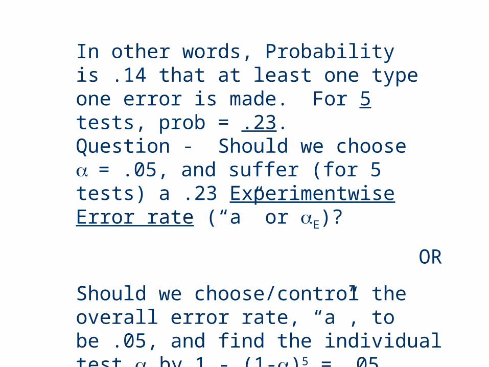
In other words, Probability is .14 that at least one type one error is made. For 5 tests, prob = .23.Question - Should we choose = .05, and suffer (for 5 tests) a .23 Experimentwise Error rate (“a” or E)?

OR

Should we choose/control the overall error rate, “a”, to be .05, and find the individual test by 1 - (1-)5 = .05, (which gives us = .011)?

The formula 1 - (1-)5 = .05

would be valid only if the tests are independent; often they’re not.

[ e.g., 1=22= 3, 1= 3

IF accepted & rejected, isn’t it more likely that rejected? ]

1 2

21

3

3

When the tests are not independent, it’s usually very difficult to arrive at the correct for an individual test so that a specified value results for the experimentwise error rate (or called family error rate).

Error Rates

There are many multiple comparison procedures. We’ll cover only a few.

Pairwise Comparisons

Method 1: (Fisher Test) Do a series of pairwise t-tests, each with specified value (for individual test).

This is called “Fisher’s LEAST SIGNIFICANT DIFFERENCE” (LSD).

Example: Broker Study

A financial firm would like to determine if brokers they use to execute trades differ with respect to their ability to provide a stock purchase for the firm at a low buying price per share. To measure cost, an index, Y, is used.

Y=1000(A-P)/AwhereP=per share price paid for the stock;A=average of high price and low price per share, for the day.“The higher Y is the better the trade is.”

}1

1235-112

5 6

27

1713117

17 12

381743

7 5

524131418141917

R=6

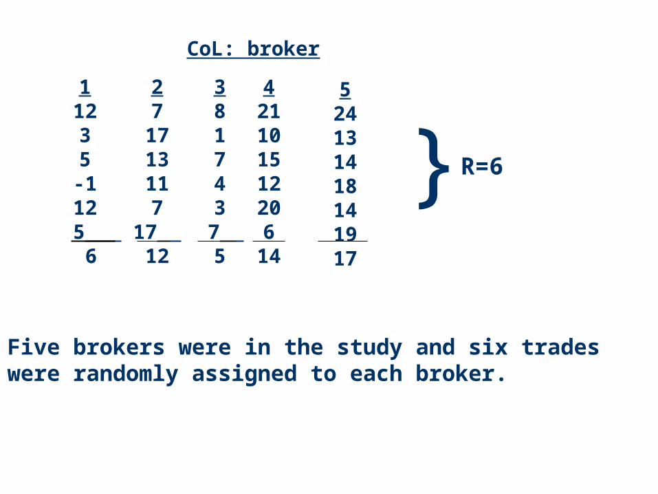
CoL: broker

421101512206

14

Five brokers were in the study and six trades were randomly assigned to each broker.

= .05, FTV = 2.76

(reject equal column MEANS)

Source SSQ df MSQ FCol

Error

640.8

530

4

25

160.2

21.2

7.56

“MSW”

0

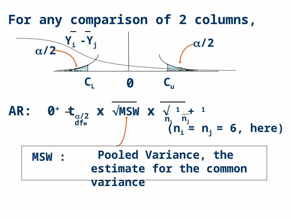
For any comparison of 2 columns,

/2/2

CL Cu

Yi -Yj

AR: 0+ t/2 x MSW x 1 + 1

ni njdfw(ni = nj = 6, here)

MSW : Pooled Variance, the estimate for the common variance

In our example, with=.05

0 2.060 (21.2 x 1 + 1 )0 5.48

6 6

This value, 5.48 is called the Least Significant Difference (LSD).

When same number of data points, R, in each column, LSD = t/2 x 2xMSW

.R

Col: 3 1 2 4 5 5 6 12 14 17

Summarize the comparison results. (p. 443)

1. Now, rank order and compare:

Underline Diagram

Step 2: identify difference > 5.48, and mark accordingly:

5 6 12 14 173 1 2 4 5

3: compare the pair of means within each subset:Comparison difference vs. LSD

3 vs. 12 vs. 42 vs. 54 vs. 5

**

*

<<<<

* Contiguous; no need to detail

5

Conclusion : 3, 1 2, 4, 5

Can get “inconsistency”: Suppose col 5 were 18:

3 1 2 4 5 5 6 12 14 18

Now: Comparison |difference| vs. LSD3 vs. 12 vs. 42 vs. 54 vs. 5

* *

*

<<><

Conclusion : 3, 1 2 4 5 ???

6

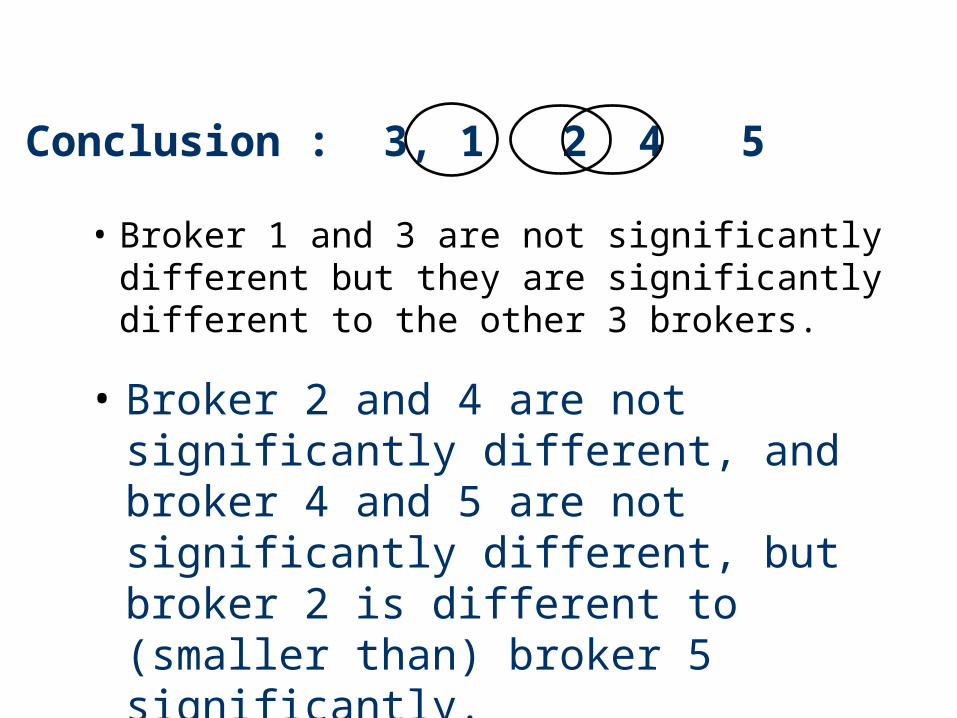
• Broker 1 and 3 are not significantly different but they are significantly different to the other 3 brokers.

Conclusion : 3, 1 2 4 5

• Broker 2 and 4 are not significantly different, and broker 4 and 5 are not significantly different, but broker 2 is different to (smaller than) broker 5 significantly.

MULTIPLE COMPARISON TESTING

AFS BROKER STUDYBROKER ----> 1 2 3 4 5TRADE 1 12 7 8 21 24 2 3 17 1 10 13 3 5 13 7 15 14 4 -1 11 4 12 18 5 12 7 3 20 14 6 5 17 7 6 19

COLUMN MEAN 6 12 5 14 17

ANOVA TABLE

SOURCE SSQ DF MS Fcalc

BROKER 640.8 4 160.2 7.56

ERROR 530 25 21.2

Fisher's pairwise comparisons (Minitab)

Family error rate = 0.268

Individual error rate = 0.0500

Critical value = 2.060 t_/2 (not given in version 16.1)

Intervals for (column level mean) - (row level mean)

1 2 3 4

2 -11.476

-0.524

3 -4.476 1.524

6.476 12.476

4 -13.476 -7.476 -14.476

-2.524 3.476 -3.524

5 -16.476 -10.476 -17.476 -8.476

-5.524 0.476 -6.524 2.476

Minitab: Stat>>ANOVA>>One-Way Anova then click “comparisons”.

Col 1 < Col 2

Col 2 = Col 4

Minitab Output for Broker Data

• Grouping Information Using Fisher Method

• broker N Mean Grouping• 5 6 17.000 A• 4 6 14.000 A• 2 6 12.000 A• 1 6 6.000 B• 3 6 5.000 B

• Means that do not share a letter are significantly different.

Pairwise comparisons

Method 2: (Tukey Test) A procedure which controls the experimentwise error rate is “TUKEY’S HONESTLY SIGNIFICANT DIFFERENCE TEST ”.

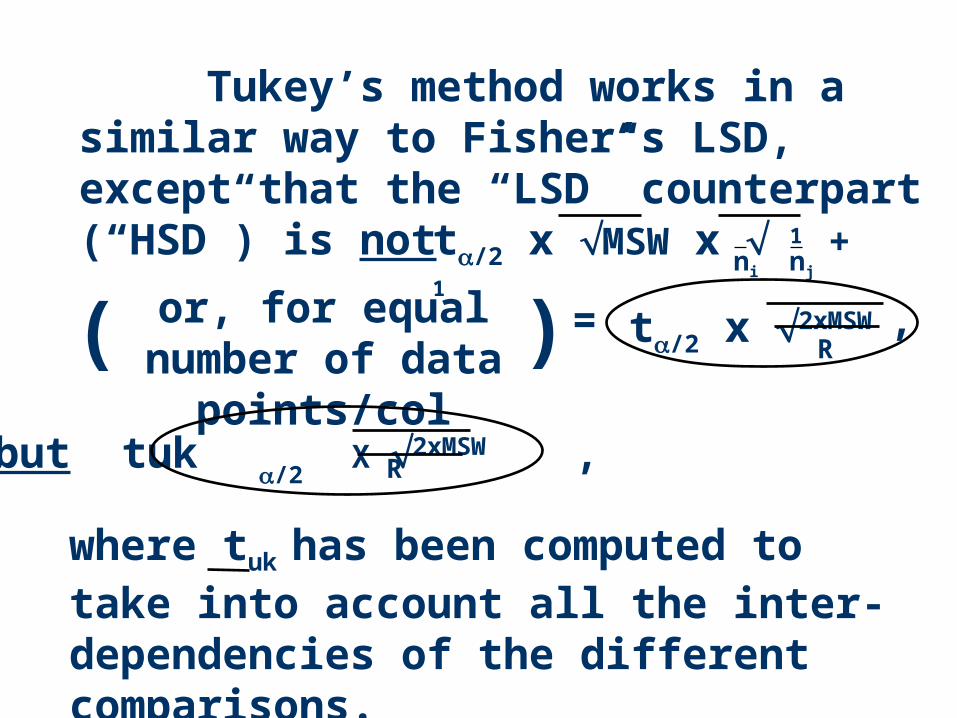
Tukey’s method works in a similar way to Fisher’s LSD, except that the “LSD” counterpart (“HSD”) is not

t/2 x MSW x 1 + 1ni nj

t/2 x 2xMSWR

=or, for equal number of data points/col( ) ,

but tuk X 2xMSW ,R

where tuk has been computed to take into account all the inter-dependencies of the different comparisons.

/2

HSD = tuk/2x2MSW R

_______________________________________

A more general approach is to write

HSD = qxMSW R

where q = tuk/2 x2

--- q = (Ylargest - Ysmallest) / MSW R

---- probability distribution of q is called the

“Studentized Range Distribution”.

--- q = q(c, df), where c =number of columns,

and df = df of MSW

With c = 5 and df = 25,from table (or Minitab):

q = 4.15tuk = 4.15/1.414 = 2.93

Then,

HSD = 4.15

alsox

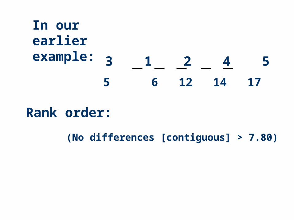
In our earlier example:

Rank order:

3 1 2 4 5

5 6 12 14 17

(No differences [contiguous] > 7.80)

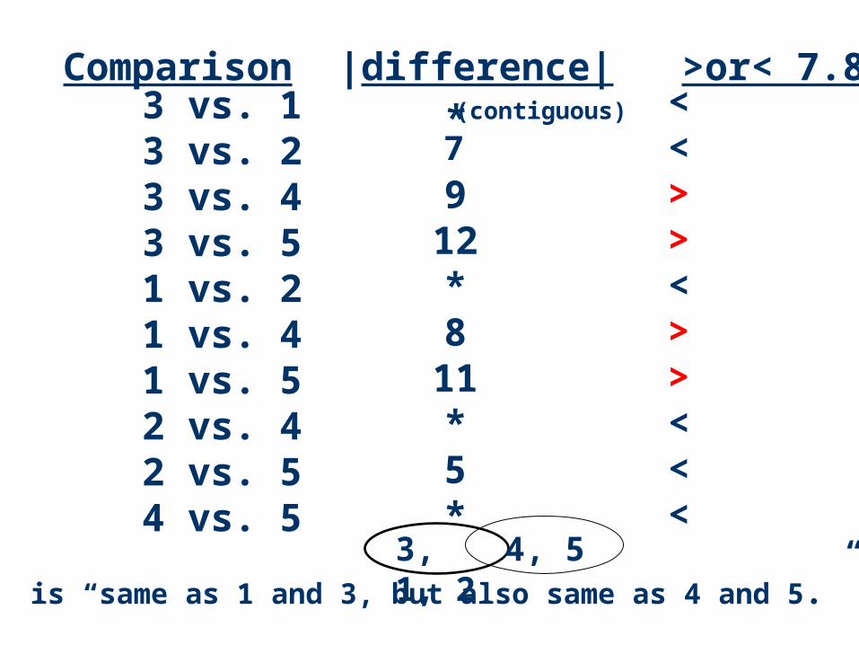
Comparison |difference| >or< 7.803 vs. 13 vs. 23 vs. 43 vs. 51 vs. 21 vs. 41 vs. 52 vs. 42 vs. 54 vs. 5

* <<>><>><<<

912*8

11*5*

(contiguous)

7

3, 1, 2 4, 52 is “same as 1 and 3, but also same as 4 and 5.”

Tukey's pairwise comparisons (Minitab)

Family error rate = 0.0500

Individual error rate = 0.00706

Critical value = 4.15 q_(not given in version 16.1)

Intervals for (column level mean) - (row level mean)

1 2 3 4 2 -13.801 1.801 3 -6.801 -0.801 8.801 14.801 4 -15.801 -9.801 -16.801 -0.199 5.801 -1.199 5 -18.801 -12.801 -19.801 -10.801 -3.199 2.801 -4.199 4.801

Minitab: Stat>>ANOVA>>One-Way Anova then click “comparisons”.

Minitab Output for Broker Data

• Grouping Information Using Tukey Method

• broker N Mean Grouping• 5 6 17.000 A• 4 6 14.000 A• 2 6 12.000 A B• 1 6 6.000 B• 3 6 5.000 B

• Means that do not share a letter are significantly different.

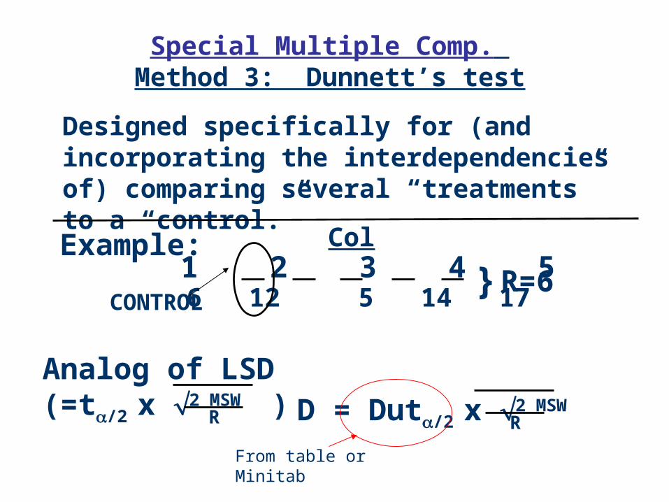
Special Multiple Comp. Method 3: Dunnett’s test

Designed specifically for (and incorporating the interdependencies of) comparing several “treatments” to a “control.”

Example: 1 2 3 4 5

6 12 5 14 17

Col

} R=6CONTROL

Analog of LSD (=t/2 x 2 MSW )R D = Dut/2 x 2 MSW

R

From table or Minitab

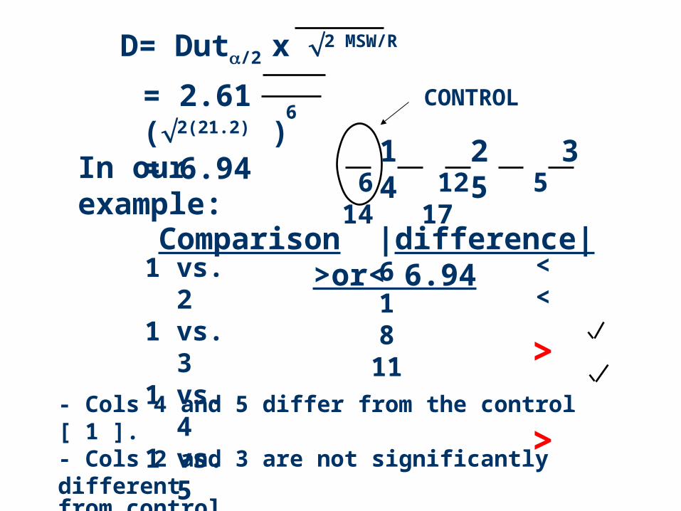
D= Dut/2 x 2 MSW/R

= 2.61 (2(21.2) )= 6.94

- Cols 4 and 5 differ from the control [ 1 ].- Cols 2 and 3 are not significantly differentfrom control.

6

In our example: 1 2 3 4 5 6 12 5 14 17

CONTROL

Comparison |difference| >or< 6.941 vs. 21 vs. 31 vs. 41 vs. 5

618

11

<< > >

Dunnett's comparisons with a control (Minitab)

Family error rate = 0.0500 controlled!!Individual error rate = 0.0152

Critical value = 2.61 Dut_/2

Control = level (1) of broker

Intervals for treatment mean minus control mean

Level Lower Center Upper --+---------+---------+---------+-----2 -0.930 6.000 12.930 (---------*--------) 3 -7.930 -1.000 5.930 (---------*--------) 4 1.070 8.000 14.930 (--------*---------) 5 4.070 11.000 17.930 (---------*---------) --+---------+---------+---------+----- -7.0 0.0 7.0 14.0

Minitab: Stat>>ANOVA>>General Linear Model then click “comparisons”.

What Method Should We Use?

Fisher procedure can be used only after the F-test in the Anova is significant at 5%.

Otherwise, use Tukey procedure. Note that to avoid being too conservative, the significance level of Tukey test can be set bigger (10%), especially when the number of levels is big.

Contrast

Example 1

1 2 3 4

Placebo

Sulfa

Type

S1

Sulfa

Type

S2

Anti-biotic

Type A

Suppose the questions of interest are

(1) Placebo vs. Non-placebo

(2) S1 vs. S2

(3) (Average) S vs. A

In general, a question of interest can be expressed by a linear combination of column means such as

with restriction that aj = 0.

Such linear combinations are called contrasts.

jj

jYaC .

Test if a contrast has mean 0The sum of squares for contrast Z is

where R is the number of rows (replicates).

The test statistic Fcalc = SSC/MSW is distributed as F with 1 and (df of error) degrees of freedom.

Reject E[C]= 0 if the observed Fcalc is too large

(say, > F0.05(1,df of error) at 5% significant level).

j

jaCRSSC 22 /

Example 1 (cont.): aj’s for the 3 contrasts

P vs. P: C1

S1 vs. S2:C2

S vs. A: C3

1 2 3 4

-3 1 1 1

0 -1 1 0

0 -1 -1 2

P S1 S2 A

top row middle row bottom row

j

ja2

Calculating

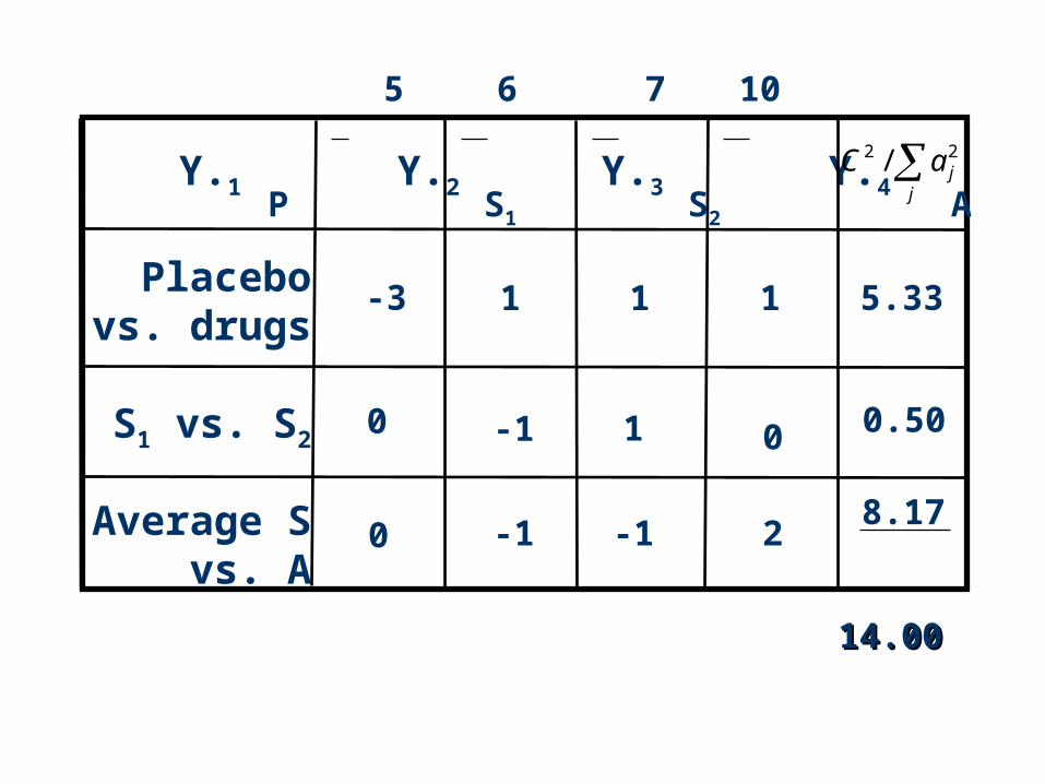
Y.1 Y.2 Y.3 Y.4

1 1 1 5.33

0.50

8.17

0

0

Placebovs. drugs

S1 vs. S2

Average Svs. A

P S1 S2 A

14.0014.00

5 6 7 10

-1

01

-1

-1

-3

2

j

jaC 22 /

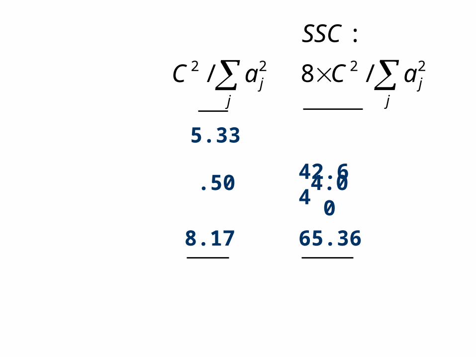
42.64

.50 4.00

8.17 65.36

5.33

j

jaC 22 / j

jaC

SSC22 /8

:

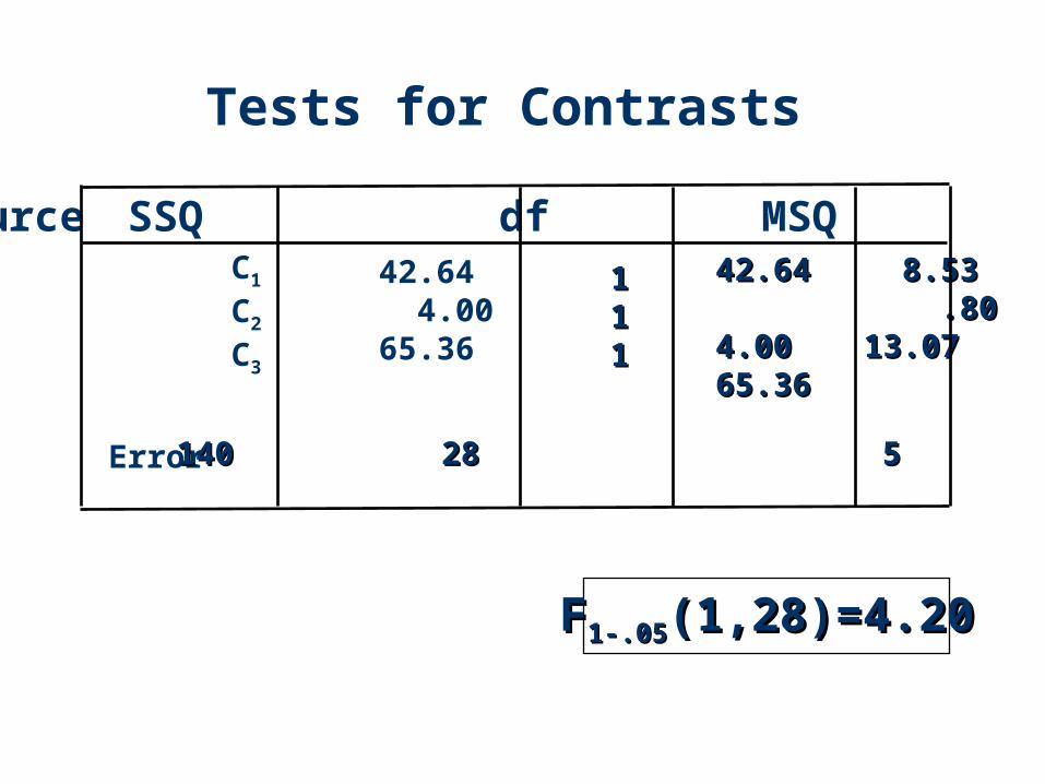
Tests for Contrasts

Source SSQ df MSQ F

Error

C1

C2

C3

42.64 4.00 65.36

111111

42.6442.64 4.004.0065.3665.36

8.538.53 .80.8013.0713.07

140140 28 5 28 5

FF1-.051-.05(1,28)=4.20(1,28)=4.20

Example 1 (Cont.): Conclusions

The mean response for Placebo is significantly different to that for Non-placebo.

There is no significant difference between using Types S1 and S2.

Using Type A is significantly different to using Type S on average.