Embed Size (px)
Citation preview

Experiments on random lasers

Experiments on random lasers
ACADEMISCH PROEFSCHRIFT
ter verkrijging van de graad van doctoraan de Universiteit van Amsterdam,op gezag van de Rector Magnificus
prof. dr. J. J. M. Franseten overstaan van een door het college voor promotiesingestelde commissie in het openbaar te verdedigen
in de Aula der Universiteitop dinsdag 4 december 2001 te 14:00 uur
door
Gijs van Soest
geboren te Assen
Promotiecommissie:
Promotor Prof. Dr. A. Lagendijk
Overige leden Prof. Dr. D. LenstraProf. Dr. H. B. van Linden van den HeuvellProf. Dr. C. M. SoukoulisDr. R. SprikProf. Dr. J. P. Woerdman
Faculteit der Natuurwetenschappen, Wiskunde en Informatica
The work described in this thesis is part of the research program of the “StichtingFundamenteel Onderzoek der Materie (FOM)”, which is financially supported by
the “Nederlandse Organisatie voor Wetenschappelijk Onderzoek (NWO)”.
It was carried out at theVan der Waals-Zeeman Instituut, Valckenierstraat 65,
1018 XE Amsterdam, The Netherlands,where a limited number of copies of this thesis is available.
Ontwerp: Miranda Ensink, Gijs van Soest.Druk: Ponsen & Looijen BV, Wageningen.
ISBN: 90-6464-648-1

C.Contents
1 Introduction: light diffusion and lasers 111.1 Waves in complex media . . . . . . . . . . . . . . . . . . . . . . . 11
1.1.1 Light interacting with matter . . . . . . . . . . . . . . . . . 121.1.2 Single particle scattering . . . . . . . . . . . . . . . . . . . 14
1.2 Light transport . . . . . . . . . . . . . . . . . . . . . . . . . . . . 161.2.1 Multiple scattering and diffusion . . . . . . . . . . . . . . . 181.2.2 Random walks . . . . . . . . . . . . . . . . . . . . . . . . 211.2.3 Anderson localization and photonic band gaps . . . . . . . 22
1.3 The laser . . . . . . . . . . . . . . . . . . . . . . . . . . . . . . . . 221.3.1 Rate equations . . . . . . . . . . . . . . . . . . . . . . . . 241.3.2 Amplified spontaneous emission . . . . . . . . . . . . . . . 281.3.3 Laser dyes . . . . . . . . . . . . . . . . . . . . . . . . . . 28
1.4 Random lasers . . . . . . . . . . . . . . . . . . . . . . . . . . . . . 301.4.1 Issues in random laser physics . . . . . . . . . . . . . . . . 301.4.2 Is it a laser? . . . . . . . . . . . . . . . . . . . . . . . . . . 32
2 Amplifying volume in scattering media 332.1 Phenomenology . . . . . . . . . . . . . . . . . . . . . . . . . . . . 34
2.1.1 Laser threshold . . . . . . . . . . . . . . . . . . . . . . . . 342.1.2 Reabsorption . . . . . . . . . . . . . . . . . . . . . . . . . 35
2.2 Qualitative explanation of the random laser threshold . . . . . . . . 372.3 Amplifying volume in scattering media . . . . . . . . . . . . . . . 38
2.3.1 Experimental method . . . . . . . . . . . . . . . . . . . . . 382.3.2 Weakly scattering medium . . . . . . . . . . . . . . . . . . 40
2.4 Random walk simulation . . . . . . . . . . . . . . . . . . . . . . . 412.5 Discussion . . . . . . . . . . . . . . . . . . . . . . . . . . . . . . . 44
7
Contents
3 Dynamics of the threshold crossing 473.1 The photon bomb . . . . . . . . . . . . . . . . . . . . . . . . . . . 483.2 Transport equations . . . . . . . . . . . . . . . . . . . . . . . . . . 493.3 β-factor in a random laser . . . . . . . . . . . . . . . . . . . . . . . 50
3.3.1 Spontaneous emission seeding in cavity and random lasers . 503.3.2 Quantitative construction of β in a random laser . . . . . . . 513.3.3 Discussion . . . . . . . . . . . . . . . . . . . . . . . . . . 53
3.4 Closer investigation of the transport equations . . . . . . . . . . . . 543.4.1 Analogy with conventional lasers . . . . . . . . . . . . . . 553.4.2 Intrinsic dynamics . . . . . . . . . . . . . . . . . . . . . . 57
3.5 Transport properties of random lasers . . . . . . . . . . . . . . . . 603.5.1 Spatial behavior . . . . . . . . . . . . . . . . . . . . . . . 623.5.2 Temporal features . . . . . . . . . . . . . . . . . . . . . . . 643.5.3 Laser threshold and the explosion . . . . . . . . . . . . . . 653.5.4 Comparison with earlier work . . . . . . . . . . . . . . . . 67
4 Interference in random lasers 714.1 Experimental considerations . . . . . . . . . . . . . . . . . . . . . 714.2 Speckle in random lasers . . . . . . . . . . . . . . . . . . . . . . . 73
4.2.1 Sample and setup . . . . . . . . . . . . . . . . . . . . . . . 744.2.2 Intensity statistics . . . . . . . . . . . . . . . . . . . . . . . 764.2.3 Speckle spot size . . . . . . . . . . . . . . . . . . . . . . . 784.2.4 Possible experiments? . . . . . . . . . . . . . . . . . . . . 80
4.3 Enhanced backscattering in random lasers . . . . . . . . . . . . . . 814.3.1 Experimental details . . . . . . . . . . . . . . . . . . . . . 824.3.2 Results from experiment . . . . . . . . . . . . . . . . . . . 834.3.3 Comparison with theory of chapter 3 . . . . . . . . . . . . . 854.3.4 Discussion . . . . . . . . . . . . . . . . . . . . . . . . . . 88
4.4 Conclusions . . . . . . . . . . . . . . . . . . . . . . . . . . . . . . 89
5 Narrow peaks in fluorescence from scattering systems 915.1 Critical review . . . . . . . . . . . . . . . . . . . . . . . . . . . . . 92
5.1.1 Observations and interpretations from the literature . . . . . 925.1.2 Localization and random ring cavities . . . . . . . . . . . . 945.1.3 Thin film “random” laser . . . . . . . . . . . . . . . . . . . 96
5.2 Experimental results . . . . . . . . . . . . . . . . . . . . . . . . . 985.2.1 ZnO powders . . . . . . . . . . . . . . . . . . . . . . . . . 985.2.2 Scattering dye solutions . . . . . . . . . . . . . . . . . . . 103
5.3 Discussion and conclusions . . . . . . . . . . . . . . . . . . . . . . 1055.3.1 ZnO powders . . . . . . . . . . . . . . . . . . . . . . . . . 106
8
Contents
5.3.2 Dye suspensions . . . . . . . . . . . . . . . . . . . . . . . 1085.3.3 Conclusions . . . . . . . . . . . . . . . . . . . . . . . . . . 109
A Properties of Sulforhodamine B and Coumarin 6 111
B Pump units and terminology 113
References 115
Summary 123
Samenvatting 127
Dankwoord 133
9

1.Introduction:
light diffusion and lasers
This thesis is about random lasers: systems in which light is both multiply scatteredand amplified. It draws on many aspects of the interaction between light and mat-ter. This chapter is a primer that introduces these aspects in such a way that thenecessary elements from laser physics and light in complex dielectric media can bebrought together in one picture of random lasers. Only the material that is actuallyused for theory and experiments is presented in a quantitative manner.
1.1 Waves in complex media
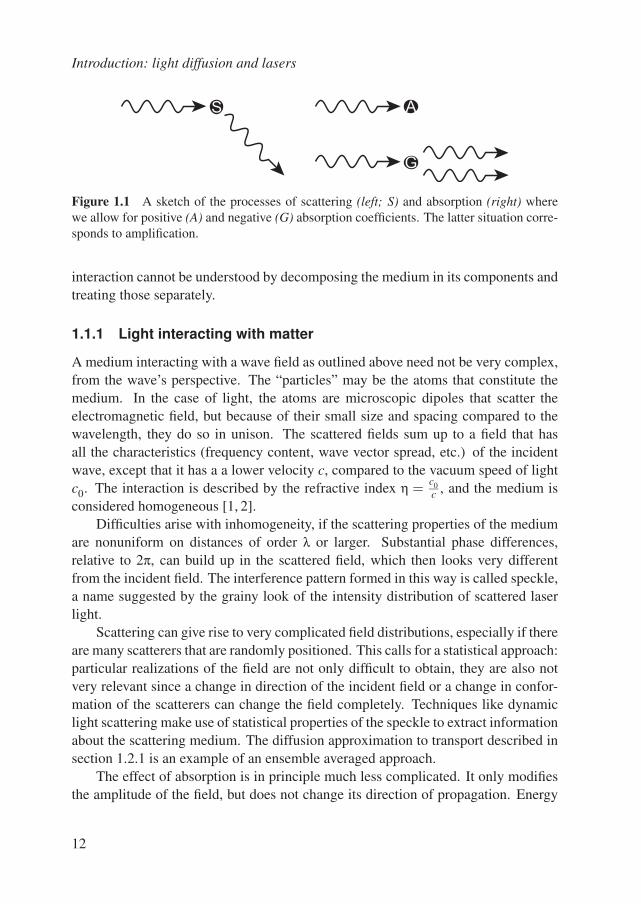
The propagation of waves in scattering media is a subject with many facets. Meteo-rology, astronomy, seismology and remote sensing are but a few of the many disci-plines that make use of the concept of wave transport in complex media. Althoughtechniques and terminology differ, the central idea is the same across al these disci-plines: while the (classical) wave travels, it interacts with “particles” in the medium.This interaction can be either scattering or absorption or both. We only considerelastic scattering: no energy is transferred to or from the wave field. Then, scat-tering is an interaction that changes the direction of propagation of the wave field,while absorption changes the amplitude of the wave, see figure 1.1. If absorption isunderstood in the usual sense, the change is downward: the amplitude diminishes.However, for the current work, we allow for a negative absorption which makes theamplitude increase, to describe gain. In this section, by absorption we mean absorp-tion in this general sense.
The word “complex” is used here to signify composite, made up of related parts.It derives from the Latin “complectere”, meaning “to embrace”. The constituentparts of the medium are inextricably mixed, and the properties of wave transportin such a medium are largely determined by its composite nature. The wave–matter
11
Introduction: light diffusion and lasers
A
G
S
Figure 1.1 A sketch of the processes of scattering (left; S) and absorption (right) wherewe allow for positive (A) and negative (G) absorption coefficients. The latter situation corre-sponds to amplification.
interaction cannot be understood by decomposing the medium in its components andtreating those separately.
1.1.1 Light interacting with matter
A medium interacting with a wave field as outlined above need not be very complex,from the wave’s perspective. The “particles” may be the atoms that constitute themedium. In the case of light, the atoms are microscopic dipoles that scatter theelectromagnetic field, but because of their small size and spacing compared to thewavelength, they do so in unison. The scattered fields sum up to a field that hasall the characteristics (frequency content, wave vector spread, etc.) of the incidentwave, except that it has a a lower velocity c, compared to the vacuum speed of lightc0. The interaction is described by the refractive index η = c0
c , and the medium isconsidered homogeneous [1, 2].
Difficulties arise with inhomogeneity, if the scattering properties of the mediumare nonuniform on distances of order λ or larger. Substantial phase differences,relative to 2π, can build up in the scattered field, which then looks very differentfrom the incident field. The interference pattern formed in this way is called speckle,a name suggested by the grainy look of the intensity distribution of scattered laserlight.
Scattering can give rise to very complicated field distributions, especially if thereare many scatterers that are randomly positioned. This calls for a statistical approach:particular realizations of the field are not only difficult to obtain, they are also notvery relevant since a change in direction of the incident field or a change in confor-mation of the scatterers can change the field completely. Techniques like dynamiclight scattering make use of statistical properties of the speckle to extract informationabout the scattering medium. The diffusion approximation to transport described insection 1.2.1 is an example of an ensemble averaged approach.
The effect of absorption is in principle much less complicated. It only modifiesthe amplitude of the field, but does not change its direction of propagation. Energy
12
1.1 Waves in complex media
1 2 3
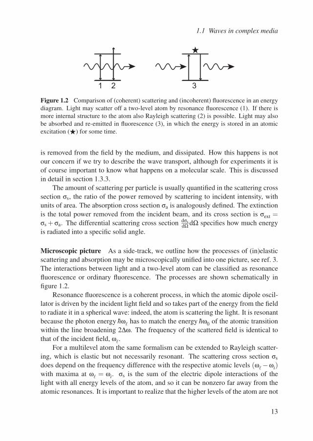
Figure 1.2 Comparison of (coherent) scattering and (incoherent) fluorescence in an energydiagram. Light may scatter off a two-level atom by resonance fluorescence (1). If there ismore internal structure to the atom also Rayleigh scattering (2) is possible. Light may alsobe absorbed and re-emitted in fluorescence (3), in which the energy is stored in an atomicexcitation () for some time.
is removed from the field by the medium, and dissipated. How this happens is notour concern if we try to describe the wave transport, although for experiments it isof course important to know what happens on a molecular scale. This is discussedin detail in section 1.3.3.
The amount of scattering per particle is usually quantified in the scattering crosssection σs, the ratio of the power removed by scattering to incident intensity, withunits of area. The absorption cross section σa is analogously defined. The extinctionis the total power removed from the incident beam, and its cross section is σext =σs + σa. The differential scattering cross section dσs
dΩ dΩ specifies how much energyis radiated into a specific solid angle.
Microscopic picture As a side-track, we outline how the processes of (in)elasticscattering and absorption may be microscopically unified into one picture, see ref. 3.The interactions between light and a two-level atom can be classified as resonancefluorescence or ordinary fluorescence. The processes are shown schematically infigure 1.2.
Resonance fluorescence is a coherent process, in which the atomic dipole oscil-lator is driven by the incident light field and so takes part of the energy from the fieldto radiate it in a spherical wave: indeed, the atom is scattering the light. It is resonantbecause the photon energy hω has to match the energy hω0 of the atomic transitionwithin the line broadening 2∆ω. The frequency of the scattered field is identical tothat of the incident field, ω.
For a multilevel atom the same formalism can be extended to Rayleigh scatter-ing, which is elastic but not necessarily resonant. The scattering cross section σs
does depend on the frequency difference with the respective atomic levels (ω −ωi)with maxima at ω = ωi. σs is the sum of the electric dipole interactions of thelight with all energy levels of the atom, and so it can be nonzero far away from theatomic resonances. It is important to realize that the higher levels of the atom are not
13
Introduction: light diffusion and lasers
populated in an intermediate state, although all atomic states contribute to the crosssection.
Ordinary fluorescence is an incoherent process in which the photon energy isfirst absorbed by the atom, stored for some time τ and then re-emitted. There is norelation between the phases of incident and radiated fields and the frequency of thelatter may be anywhere within the broadened atomic transition line ω0 ±∆ω. Theemitted field is not part of the scattered field as originating from elastic processes.
1.1.2 Single particle scattering
The particles that are the scatterers may interact with light in different ways, de-pending on their size. For light scattering, three qualitatively distinct ranges areimportant: Rayleigh scattering, Mie scattering, and geometric optics. We mentionedalready that atoms can scatter light (Rayleigh scattering; the first range). The scat-tering by an ensemble of atoms can be written as the product of the single atomscattering cross section and a structure factor that arises from the summed scatteredfields of individual atoms [4]. For an ensemble much larger than λ consisting ofmany closely spaced ( λ) atoms the structure factor is zero except in the forwarddirection, the spherical waves emanating from each atom cancel in all other direc-tions. This is a homogeneous medium as described on page 12, and we can applygeometric optics (the third range). In Mie scattering (the second range), particleswith a size of about a wavelength can produce strong resonances in the structurefactor due to interference in the scattered field.
Scattering is characterized by two important numbers: the size parameter x ofthe particle and the refractive index contrast m.
x = ka ≡ 2πηaλ
; m ≡ η1
η; (1.1)
where a is the “radius” of the particle (see the paragraphs on Mie scattering belowfor refining considerations about the shape of the particle), and η and η1 are therefractive indices of medium and scatterer, respectively.
Rayleigh scattering Scattering of light by particles much smaller than the wave-length (x, mx 1), such as atoms, molecules, and very fine dust, is called Rayleighscattering. Its hallmark is the proportionality of the scattering cross section to 1/λ4,of which several derivations can be found in the literature (different formulations aregiven in refs. 3, 5–7). We paraphrase the elegant consideration by Lord Rayleighhimself [8]:
A dimensionless ratio between scattered and incident field may depend onthese quantities: volume V of the particle, position r, wave velocity c, dielectric
14
1.1 Waves in complex media
(b)(a)
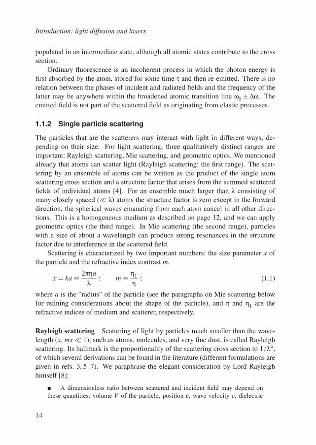
Figure 1.3 Sketches of scattering (a) in the Rayleigh limit, and (b) in the geometric opticslimit. In (a) the scatterer takes out a part of the incident plane wave and radiates it as aspherical scattered wave. In (b) the scatterer is large enough (x 1) to allow drawing thelight as a ray inside. As an example a whispering gallery mode of a disk or sphere, excitedby the incident wave, is shown.
constants of sphere ε1 and surroundings ε0, and wavelength λ with appropriateunits. c is the only one with a unit containing time and thus can not play a role,the dielectric constants have units involving capacitance and thus can only appearas ε1/ε0, which leaves the ratio V/(rλ2) as the only candidate (compatible with theknown 1/r decay of the amplitude). Squaring this to get the ratio between scatteredand incident energy reveals a proportionality to 1/λ4.
The dielectric constant of the scatterer appears (for ε0 = 1) as the factor V ε1−1ε1+2 ,
the static polarizability of a small dielectric sphere.As is well known, scattering of light in the atmosphere is accurately described
by Rayleigh scattering. The strong dependence on the wavelength causes blue lightto be scattered about 6 times more efficiently than red light, accounting for the bluesky and the red sun at sunset.
Mie scattering If x is of order 1 the problem of scattering can only be solved by aformal solution of Maxwell’s equations with appropriate boundary conditions. Thereis no short route towards physical insight [9], other than the handwaving argumentgiven by Feynman [10], summarized below:
The N microscopic dipoles that make up a scatterer radiate in phase if they arewithin half a wavelength of each other, which produces a scattered field that is Ntimes the field of one dipole due to constructive interference. Thus the scatteredenergy from this collection of N dipoles is (N ·1)2 = N2 times the field of 1, com-pared to a scattered energy of N · (1)2 = N if the phases are independent. Thisindicates that scattering in this regime can be very strong, with sharp resonances asa function of x and m. In these resonances, σs can become as large as λ2 (severaltimes the geometric cross section of the scatterer), and there is considerable angularstructure in the differential cross section.
15
Introduction: light diffusion and lasers
The problem can only be exactly solved for certain simple shapes such as asphere or a cylinder. Scattering by a sphere of arbitrary size is called Mie scattering,after one of the early physicists who worked on the problem. An extensive treatmentof the problem is given in ref. 11. The scatterers used in our experiments do fall in therange of x ≈ 1, but they are irregularly shaped, all different and polydisperse, insteadof being spheres of equal size. The detailed results of Mie theory are thereforeof limited use. We content ourselves with noticing that our particles are stronglyscattering and that every particle has a different cross section, the details of whichwill not affect the experimental results.
Geometric optics For scatterers much larger than the wavelength, geometric (ray)optics can be used for the propagation of the intensity, if necessary with appropriatecorrections for the wave character of light. The light can be pictured as a ray insidethe material. This need not at all be trivial or dull, as is witnessed by natural marvelslike the rainbow [12] or devices like microsphere lasers [13] (lasing on a whisperinggallery mode, see figure 1.3b), both of which can be described to a certain extent bygeometric optics.
1.2 Light transport
To incorporate all of the diversity outlined above into a comprehensive transporttheory for light traveling through matter, consisting of many particles interactingwith the light in various ways, is certainly a formidable task. Also, such a theorywill be unpractical for describing actual experiments because of its involved nature;it may be correct, but also very cumbersome.
In order to be able to describe transport, a distinction in several regimes is madedepending on how strongly the interaction with the medium changes the wave field.We then work with an approximate version of transport theory that suits the regimeof the physical system under study. Two quantities determine the magnitude of theeffect on the light: the strength of the interaction X (X is “s” for scattering or “a” forabsorption) of one particle with the field, and the number of particles. The former isquantified as the cross section σX , the latter as the particle density n.
κX = nσX or its inverse X =1
nσX(1.2)
quantify how strongly the material influences the wave field by the interaction X . κXis called the coefficient of the interaction. It has the dimensions of inverse length.Every slice dz of the medium that is traversed takes out a proportional fraction of the
16
1.2 Light transport
inte
nsity
zlx
medium
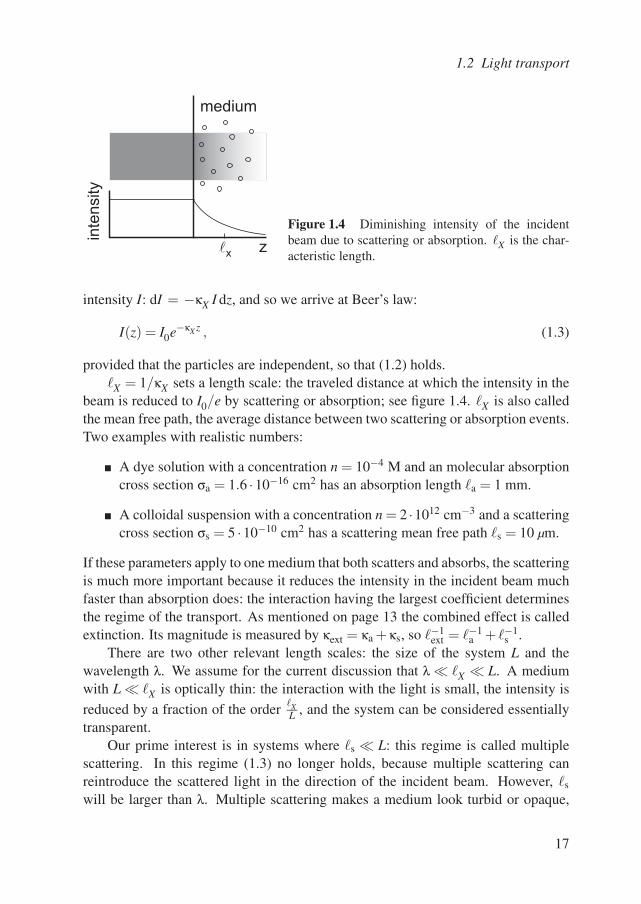
Figure 1.4 Diminishing intensity of the incidentbeam due to scattering or absorption. X is the char-acteristic length.
intensity I: dI = −κX I dz, and so we arrive at Beer’s law:
I(z) = I0e−κX z , (1.3)
provided that the particles are independent, so that (1.2) holds.X = 1/κX sets a length scale: the traveled distance at which the intensity in the
beam is reduced to I0/e by scattering or absorption; see figure 1.4. X is also calledthe mean free path, the average distance between two scattering or absorption events.Two examples with realistic numbers:
A dye solution with a concentration n = 10−4 M and an molecular absorptioncross section σa = 1.6 ·10−16 cm2 has an absorption length a = 1 mm.
A colloidal suspension with a concentration n = 2 ·1012 cm−3 and a scatteringcross section σs = 5 ·10−10 cm2 has a scattering mean free path s = 10 µm.
If these parameters apply to one medium that both scatters and absorbs, the scatteringis much more important because it reduces the intensity in the incident beam muchfaster than absorption does: the interaction having the largest coefficient determinesthe regime of the transport. As mentioned on page 13 the combined effect is calledextinction. Its magnitude is measured by κext = κa +κs, so −1
ext = −1a + −1
s .There are two other relevant length scales: the size of the system L and the
wavelength λ. We assume for the current discussion that λ X L. A mediumwith L X is optically thin: the interaction with the light is small, the intensity isreduced by a fraction of the order X
L , and the system can be considered essentiallytransparent.
Our prime interest is in systems where s L: this regime is called multiplescattering. In this regime (1.3) no longer holds, because multiple scattering canreintroduce the scattered light in the direction of the incident beam. However, s
will be larger than λ. Multiple scattering makes a medium look turbid or opaque,
17
Introduction: light diffusion and lasers
and white if it is nonabsorbing and if all wavelengths are scattered equally. Thepropagation direction of the light is continuously changed, causing incident light tobe partly scattered back towards its source. In a transparent medium light travelsin straight lines, so we can see through it. An absorbing medium removes certainwavelengths from the incident spectrum, but the propagation direction of the light isnot affected (apart from refraction), so it is transparent, only not for all colours.
If X < λ, the situation is totally different. The interaction takes effect withinone wavelength and affects the transport very strongly. Such a strong absorption(a < λ), for instance, is coupled to a high conductivity as in a metal which makesit reflecting [14]. There is, therefore, hardly any energy carried by the wave insidethe material, and the small amount that is, is dissipated. If the material is verystrongly scattering, with s < λ, interference needs to be taken into account even afterensemble averaging because the energy transport by the wave field is affected. Toappreciate the physics of very strong multiple scattering, we first need to introducediffusion of light. We return briefly to the modification of wave transport due tointerference in very strongly scattering media in section 1.2.3.
1.2.1 Multiple scattering and diffusion
In this section we will work out the situation where λ s L, we use refs. 15 and16 as a basis. λ s L means that (in an averaged description) we can disregardthe wave character of the light, and that the light encounters many scattering eventsin the medium. We further assume a random distribution of scatterers, we will touchbriefly upon ordered media in section 1.2.3.
The transport can be considered as light particles with a certain distribution inspace on a more-or-less random walk with a step length equal to the scattering meanfree path. The degree of randomness in the walk depends on how strongly each scat-tering event changes the direction of the walk, and so on the differential scatteringcross section. Mie scattering, for example, is primarily in the forward direction; ittakes a few scatterings to randomize the direction of the light.
The walk can be made really random be adopting a different step length: thetransport mean free path , the length after which the light has lost its initial directioncompletely. Unlike s, it accounts for the direction light is scattered into.
=s
1−〈cosθ〉 , (1.4)
where 〈cosθ〉 is the average cosine of the scattering angle, which can be found fromthe differential cross section. Rayleigh scattering is an example of 〈cosθ〉 = 0 or = s, while Mie scattering may have 〈cosθ〉 ≈ 0.5, so = 2s. For diffusion of
18
1.2 Light transport
the intensity, is the important length scale. We are interested in the regime where L, so the light transport is truly diffusive.
Since the propagation on length scales is random, there is a net flow of lightonly if there is nonuniform density, otherwise all microscopic propagation cancels.In order to find a description of the transport in this situation, we turn to the continu-ity equation, expressing conservation of energy in transport:
∂W∂ t
+∇ ·J = S , (1.5)
We work with “particle” densities by normalizing the field energy density and currentdensity to the photon energy. Then W is the energy density in m−3, J is the currentdensity in m−2s−1, and S is the source of diffusing light. The current density is thenet flow of light into a small volume surrounding the point we consider, per areaper time. Since the flow is driven by the density variations, the simplest possibledependence is given by Fick’s law:
J = −D∇W . (1.6)
D is the diffusion constant in m2s−1. It determines the magnitude of macroscopiclight transport, and the link with the microscopic propagation velocity c [17] and thetransport mean free path is:
D = 13 c . (1.7)
Combining (1.5) and (1.6), we arrive at the diffusion equation:
∂W∂ t
= D∇2W +S . (1.8)
This equation is valid for conservative systems, i.e. in absence of any absorption.It shows immediately that the density itself is a dynamic quantity: in a stationarysituation, we are left with ∇ ·J = S, and only the constant current can be obtained.This is used in total transmission measurements [18], for example. The source isoften a directional beam that is gradually, after one of travel into the medium,originating the diffusing density. It can be realistically modeled by an exponentiallydecaying term, similar to (1.3).
Absorption can be taken into account as a special kind of sink (a negativesource), one that is proportional to the local intensity:
∂W∂ t
= D∇2W −κacW +S . (1.9)
Gain is incorporated by a similar term with a negative κa.
19
Introduction: light diffusion and lasers
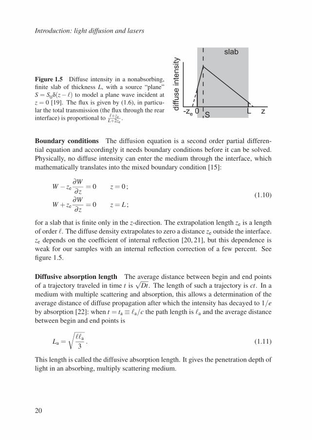
Figure 1.5 Diffuse intensity in a nonabsorbing,finite slab of thickness L, with a source “plane”S = S0δ(z− ) to model a plane wave incident atz = 0 [19]. The flux is given by (1.6), in particu-lar the total transmission (the flux through the rearinterface) is proportional to +ze
L+2ze.
diffu
se inte
nsity
z0 LS
-ze
slab
Boundary conditions The diffusion equation is a second order partial differen-tial equation and accordingly it needs boundary conditions before it can be solved.Physically, no diffuse intensity can enter the medium through the interface, whichmathematically translates into the mixed boundary condition [15]:
W − ze∂W∂ z
= 0 z = 0 ;
W + ze∂W∂ z
= 0 z = L ;(1.10)
for a slab that is finite only in the z-direction. The extrapolation length ze is a lengthof order . The diffuse density extrapolates to zero a distance ze outside the interface.ze depends on the coefficient of internal reflection [20, 21], but this dependence isweak for our samples with an internal reflection correction of a few percent. Seefigure 1.5.
Diffusive absorption length The average distance between begin and end pointsof a trajectory traveled in time t is
√Dt. The length of such a trajectory is ct. In a
medium with multiple scattering and absorption, this allows a determination of theaverage distance of diffuse propagation after which the intensity has decayed to 1/eby absorption [22]: when t = ta ≡ a/c the path length is a and the average distancebetween begin and end points is
La =
√a
3. (1.11)
This length is called the diffusive absorption length. It gives the penetration depth oflight in an absorbing, multiply scattering medium.
20
1.2 Light transport
02
46
810
12
-30
-20
-10
0
-15
-10
-5
0
z/
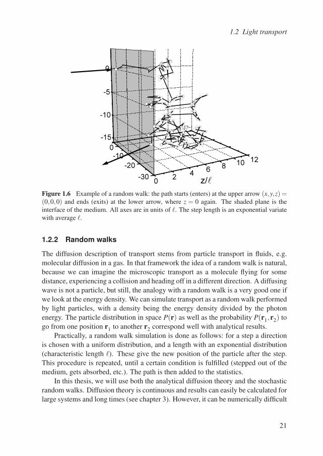
Figure 1.6 Example of a random walk: the path starts (enters) at the upper arrow (x,y,z) =(0,0,0) and ends (exits) at the lower arrow, where z = 0 again. The shaded plane is theinterface of the medium. All axes are in units of . The step length is an exponential variatewith average .
1.2.2 Random walks
The diffusion description of transport stems from particle transport in fluids, e.g.molecular diffusion in a gas. In that framework the idea of a random walk is natural,because we can imagine the microscopic transport as a molecule flying for somedistance, experiencing a collision and heading off in a different direction. A diffusingwave is not a particle, but still, the analogy with a random walk is a very good one ifwe look at the energy density. We can simulate transport as a random walk performedby light particles, with a density being the energy density divided by the photonenergy. The particle distribution in space P(r) as well as the probability P(r1,r2) togo from one position r1 to another r2 correspond well with analytical results.
Practically, a random walk simulation is done as follows: for a step a directionis chosen with a uniform distribution, and a length with an exponential distribution(characteristic length ). These give the new position of the particle after the step.This procedure is repeated, until a certain condition is fulfilled (stepped out of themedium, gets absorbed, etc.). The path is then added to the statistics.
In this thesis, we will use both the analytical diffusion theory and the stochasticrandom walks. Diffusion theory is continuous and results can easily be calculated forlarge systems and long times (see chapter 3). However, it can be numerically difficult
21
Introduction: light diffusion and lasers
to apply in situations with variation in more than one spatial dimension (e.g., a finitebeam width). In such a situation we use a Monte Carlo random walk simulation (seesection 2.4). The problem is studied stochastically by launching many walks andkeeping track of where they go to get a statistical answer to the question we pose.It can be conveniently implemented in any geometry, but since every step has to becalculated and stored separately, it is unwieldy for getting dynamic results for longtimes, and accordingly, for large systems.
1.2.3 Anderson localization and photonic band gaps
If the scattering is so strong that ks < 1, where k = 2πλ , destructive interference be-
tween scattered waves inhibits the propagation of waves over length scales largerthan the localization length: D → 0. This phenomenon is called Anderson localiza-tion, after its discoverer [23]. Localization of classical waves [24] is briskly pursuedexperimentally [25–27], by matching the scale of the inhomogeneity to the wave-length, and by increasing the refractive index contrast.
In ordered inhomogeneous dielectrics, a similar effect may occur. The multiplyscattered waves form an electromagnetic Bloch wave due to the periodicity. The iri-descence of opals is Bragg reflection of light in an ordered dielectric with a variationin the refractive index on the order of the wavelength of light: opals are an exampleof photonic crystals. A stronger interaction (larger dielectric contrast) broadens theBragg reflections, and if they cover all angles for a certain frequency, light propaga-tion at that frequency is inhibited in the crystal [28]. This phenomenon is called aphotonic bandgap, and it is intensely sought after [29].
1.3 The laser
In order to understand what happens in a random laser, a good understanding ofconventional lasers, especially of the laser threshold is needed. The basic conceptsare presented here in such a way that they can easily be adapted for use with therandom case. Laser is an acronym for light amplification by stimulated emission ofradiation. There are basically two functional parts in a laser: a light amplifier anda feedback mechanism. In conventional lasers (random lasers will be introduced insection 1.4) the feedback mechanism is an optical cavity, consisting of high qualitymirrors. Gain media come in many varieties; dyes are described in more detail insection 1.3.3. A schematic is shown in figure 1.7.
The cavity is in its simplest form a Fabry-Perot resonator of length L, the longi-tudinal modes of which are standing waves, which undergo a phase shift of an integertimes 2π in one round trip through the cavity. Light in a cavity mode experiences
22
1.3 The laser
M
G
M
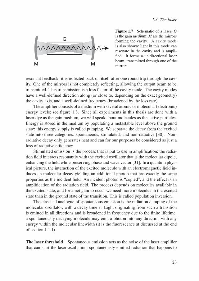
Figure 1.7 Schematic of a laser: Gis the gain medium; M are the mirrorsforming the cavity. A cavity modeis also shown: light in this mode canresonate in the cavity and is ampli-fied. It forms a unidirectional laserbeam, transmitted through one of themirrors.
resonant feedback: it is reflected back on itself after one round trip through the cav-ity. One of the mirrors is not completely reflecting, allowing the output beam to betransmitted. This transmission is a loss factor of the cavity mode. The cavity modeshave a well-defined direction along (or close to, depending on the exact geometry)the cavity axis, and a well-defined frequency (broadened by the loss rate).
The amplifier consists of a medium with several atomic or molecular (electronic)energy levels: see figure 1.8. Since all experiments in this thesis are done with alaser dye as the gain medium, we will speak about molecules as the active particles.Energy is stored in the medium by populating a metastable level above the groundstate; this energy supply is called pumping. We separate the decay from the excitedstate into three categories: spontaneous, stimulated, and non-radiative [30]. Non-radiative decay only generates heat and can for our purposes be considered as just aloss of radiative efficiency.
Stimulated emission is the process that is put to use in amplification: the radia-tion field interacts resonantly with the excited oscillator that is the molecular dipole,enhancing the field while preserving phase and wave vector [31]. In a quantum phys-ical picture, the interaction of the excited molecule with an electromagnetic field in-duces an molecular decay yielding an additional photon that has exactly the sameproperties as the incident field. An incident photon is “copied”, and the effect is anamplification of the radiation field. The process depends on molecules available inthe excited state, and for a net gain to occur we need more molecules in the excitedstate than in the ground state of the transition. This is called population inversion.
The classical analogue of spontaneous emission is the radiation damping of themolecular oscillator, with a decay time τ. Light originating from such a transitionis emitted in all directions and is broadened in frequency due to the finite lifetime:a spontaneously decaying molecule may emit a photon into any direction with anyenergy within the molecular linewidth (it is the fluorescence at discussed at the endof section 1.1.1).
The laser threshold Spontaneous emission acts as the noise of the laser amplifierthat can start the laser oscillation: spontaneously emitted radiation that happens to
23
Introduction: light diffusion and lasers
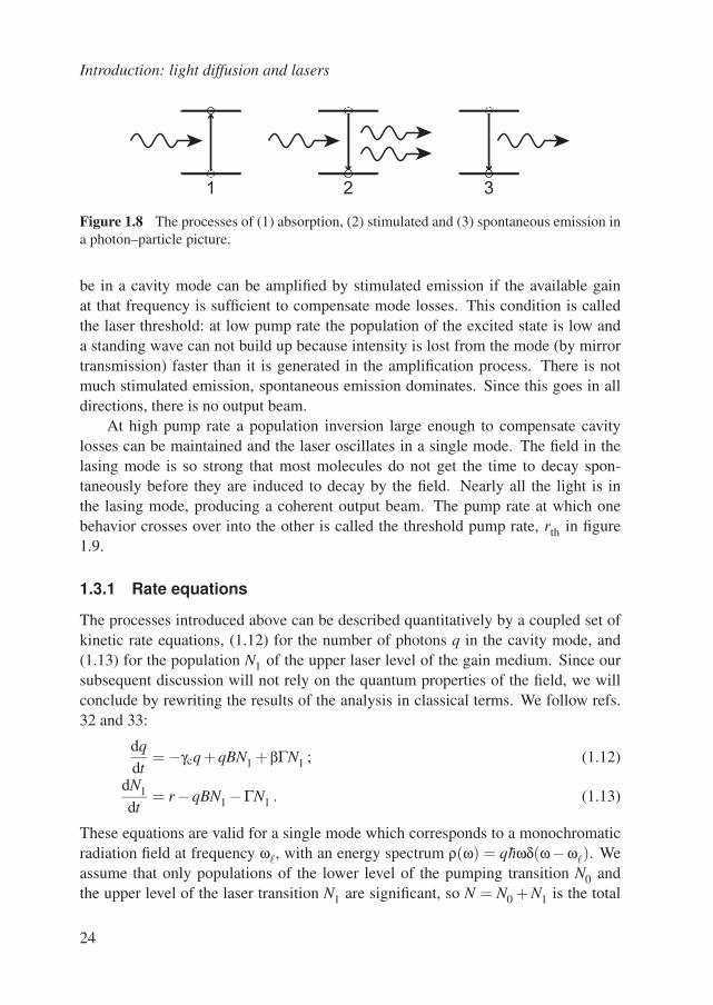
1 2 3
Figure 1.8 The processes of (1) absorption, (2) stimulated and (3) spontaneous emission ina photon–particle picture.
be in a cavity mode can be amplified by stimulated emission if the available gainat that frequency is sufficient to compensate mode losses. This condition is calledthe laser threshold: at low pump rate the population of the excited state is low anda standing wave can not build up because intensity is lost from the mode (by mirrortransmission) faster than it is generated in the amplification process. There is notmuch stimulated emission, spontaneous emission dominates. Since this goes in alldirections, there is no output beam.
At high pump rate a population inversion large enough to compensate cavitylosses can be maintained and the laser oscillates in a single mode. The field in thelasing mode is so strong that most molecules do not get the time to decay spon-taneously before they are induced to decay by the field. Nearly all the light is inthe lasing mode, producing a coherent output beam. The pump rate at which onebehavior crosses over into the other is called the threshold pump rate, rth in figure1.9.
1.3.1 Rate equations
The processes introduced above can be described quantitatively by a coupled set ofkinetic rate equations, (1.12) for the number of photons q in the cavity mode, and(1.13) for the population N1 of the upper laser level of the gain medium. Since oursubsequent discussion will not rely on the quantum properties of the field, we willconclude by rewriting the results of the analysis in classical terms. We follow refs.32 and 33:
dqdt
= −γcq+qBN1 +βΓN1 ; (1.12)
dN1
dt= r−qBN1 −ΓN1 . (1.13)
These equations are valid for a single mode which corresponds to a monochromaticradiation field at frequency ω, with an energy spectrum ρ(ω) = qhωδ(ω−ω). Weassume that only populations of the lower level of the pumping transition N0 andthe upper level of the laser transition N1 are significant, so N = N0 + N1 is the total
24
1.3 The laser
0 rth
0
q
n1
r
n1,
q
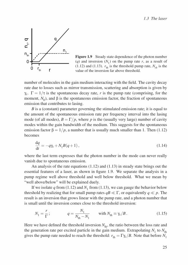
nth Figure 1.9 Steady state dependence of the photon number
(q) and inversion (N1) on the pump rate r, as a result of(1.12) and (1.13). rth is the threshold pump rate, Nth is thevalue of the inversion far above threshold.
number of molecules in the gain medium interacting with the field. The cavity decayrate due to losses such as mirror transmission, scattering and absorption is given byγc. Γ = 1/τ is the spontaneous decay rate, r is the pump rate (comprising, for themoment, N0), and β is the spontaneous emission factor, the fraction of spontaneousemission that contributes to lasing.
B is a (constant) parameter governing the stimulated emission rate; it is equal tothe amount of the spontaneous emission rate per frequency interval into the lasingmode (of all modes), B = Γ/p, where p is the (usually very large) number of cavitymodes within the gain bandwidth of the medium. This suggests for the spontaneousemission factor β = 1/p, a number that is usually much smaller than 1. Then (1.12)becomes
dqdt
= −qγc +N1B(q+1) , (1.14)
where the last term expresses that the photon number in the mode can never reallyvanish due to spontaneous emission.
An analysis of the rate equations (1.12) and (1.13) in steady state brings out theessential features of a laser, as shown in figure 1.9. We separate the analysis in apump regime well above threshold and well below threshold. What we mean by“well above/below” will be explained duely.
If we isolate q from (1.12) and N1 from (1.13), we can gauge the behavior belowthreshold by realizing that for small pump rates qB Γ, or equivalently q p. Theresult is an inversion that grows linear with the pump rate, and a photon number thatis small until the inversion comes close to the threshold inversion:
N1 =rΓ
; q =N1
Nth −N1with Nth ≡ γc/B . (1.15)
Here we have defined the threshold inversion Nth, the ratio between the loss rate andthe generation rate per excited particle in the gain medium. Extrapolating N1 to Nthgives the pump rate needed to reach the threshold: rth = Γγc/B. Note that before N1
25
Introduction: light diffusion and lasers
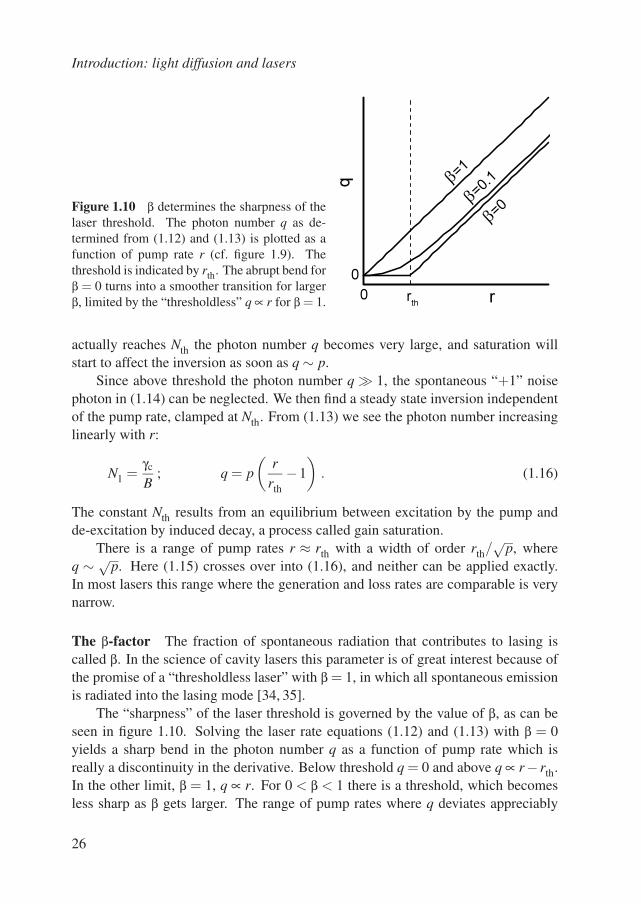
Figure 1.10 β determines the sharpness of thelaser threshold. The photon number q as de-termined from (1.12) and (1.13) is plotted as afunction of pump rate r (cf. figure 1.9). Thethreshold is indicated by rth. The abrupt bend forβ = 0 turns into a smoother transition for largerβ, limited by the “thresholdless” q ∝ r for β = 1.
=1
=0.1
=0
rth
0
0
q
r
actually reaches Nth the photon number q becomes very large, and saturation willstart to affect the inversion as soon as q ∼ p.
Since above threshold the photon number q 1, the spontaneous “+1” noisephoton in (1.14) can be neglected. We then find a steady state inversion independentof the pump rate, clamped at Nth. From (1.13) we see the photon number increasinglinearly with r:
N1 =γc
B; q = p
(r
rth−1
). (1.16)
The constant Nth results from an equilibrium between excitation by the pump andde-excitation by induced decay, a process called gain saturation.
There is a range of pump rates r ≈ rth with a width of order rth/√
p, whereq ∼ √
p. Here (1.15) crosses over into (1.16), and neither can be applied exactly.In most lasers this range where the generation and loss rates are comparable is verynarrow.
The β-factor The fraction of spontaneous radiation that contributes to lasing iscalled β. In the science of cavity lasers this parameter is of great interest because ofthe promise of a “thresholdless laser” with β = 1, in which all spontaneous emissionis radiated into the lasing mode [34, 35].
The “sharpness” of the laser threshold is governed by the value of β, as can beseen in figure 1.10. Solving the laser rate equations (1.12) and (1.13) with β = 0yields a sharp bend in the photon number q as a function of pump rate which isreally a discontinuity in the derivative. Below threshold q = 0 and above q ∝ r− rth.In the other limit, β = 1, q ∝ r. For 0 < β < 1 there is a threshold, which becomesless sharp as β gets larger. The range of pump rates where q deviates appreciably
26
1.3 The laser
from the β = 0 line is the threshold crossing region that is not described by (1.15)and (1.16). For β = 1 this holds for all pump rates.
In this description of a laser, no use was made of the resonant property of the feed-back, or the coherence of the field. Nor was the existence of other modes taken intoaccount. These refinements are important in a careful analysis of a cavity laser sys-tem but not for a random laser. The current discussion is limited to the demonstrationof the principle. The extreme multimode nature of a random laser will be taken intoaccount in β, see section 3.3.
For the discussions presented in this thesis, primarily those in chapter 3, we areinterested in the energy density of the laser field. The energy density u is related tothe (expectation value of the) photon number q by u = hω〈q〉/V , with V the modevolume [36]. We assume 〈q〉 1, so that u can be taken continuous, and normalizeu to the photon energy to obtain W = u/(hω), an energy density in units m−3. Thepopulation density for level x is obtained in a similar way: nx = Nx/V .
The pump rate r = Rn0 and the value of B need to be connected to experimentalparameters. For r this relation depends on the pumping mechanism, and we chooseto leave it unspecified until chapter 3. B is replaced by B′, the stimulated emissionrate at unit energy density. It is related to the frequency dependent stimulated emis-sion cross section, and has to be normalized to the density of modes instead of p nowthat we work with the energy density [37].
B′ =π2c3
ω2
Γg(ω0,ω) = σe(ω)c , (1.17)
with g(ω0,ω) the function describing the emission lineshape centered at ω0. Then(1.12) and (1.13) turn into
dWdt
= −γcW +σecn1W +βΓn1 ; (1.18)
dn1
dt= n0R−σecn1W −Γn1 . (1.19)
The energy and inversion densities below and above threshold, (1.15) and (1.16), arescaled accordingly.
One remark about the energy density is in order: below threshold the characteris-tics of the (intrinsically quantum) spontaneous emission noise dominate those of the(classical) coherent cavity field. This implies that a continuum description cannotbe used to adequately describe the below threshold regime, unless, strictly speaking,β = 0. We use W below threshold as a macroscopic, more or less phenomenolog-ical quantity, considering only its magnitude and do not discuss its fluctuations orcoherence properties, which are the domain of true quantum descriptions.
27
Introduction: light diffusion and lasers
a
L
ASEspont. em.
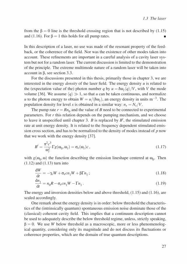
Figure 1.11 “Mirrorless lasing” in an amplifier of length L and width a. Spontaneousemission along the length is amplified, producing a narrow ASE beam.
1.3.2 Amplified spontaneous emission
In absence of a cavity, spontaneous emission is also amplified by a single passthrough the gain medium. If the amplification factor is large, as may occur in highgain systems or long amplifiers, this amplified spontaneous emission (ASE) mayshare some properties with laser light [38], such as a “laser” threshold, a directionalbeam and (limited) coherence, even though there is no feedback, let alone resonantfeedback. Another term for this phenomenon is mirrorless lasing, and its propertiesare discussed quantitatively in ref. 39.
The shape of an amplifying medium can impose a preferred direction on the ra-diation it emits. As figure 1.11 shows, spontaneous emission along the long axis ofan amplifier experiences a larger amplification than that in other directions, produc-ing a beam of ASE with a divergence depending on the length (aspect ratio L/a) ofthe amplifier. The spectrum is also narrower than the spontaneous emission spec-trum because the gain curve σe(λ) has a maximum, around which the amplificationis strongest. This is the process of gain narrowing.
The ASE threshold behavior arises from saturation: if the intensity of the travel-ing wave in the amplifier becomes large enough to extract all the stored energy (thesaturation intensity Isat = hω
σeτ [40]), the output intensity grows linearly with pumppower, like in an ordinary laser. Below Isat (shorter amplifier or lower gain) sponta-neous emission into the other directions carries off part of the energy and the outputintensity grows more slowly. This threshold is “softer” than a laser threshold pro-duced by feedback in a cavity, but for long and thin amplifiers, the difference can behard to tell. X-ray lasers, consisting of an elongated high gain plasma, are based onASE [41], because of the lack of good mirrors in that wavelength range.
1.3.3 Laser dyes
A gain medium that is used in many practical systems is a dye solution. It consists oforganic fluorescent molecules in water or an organic solvent. A dye can exhibit veryhigh gain and can be pumped efficiently, due to the large emission and absorption
28
1.3 The laser
ωp ωl
S0
S1
0
0*
1
1*
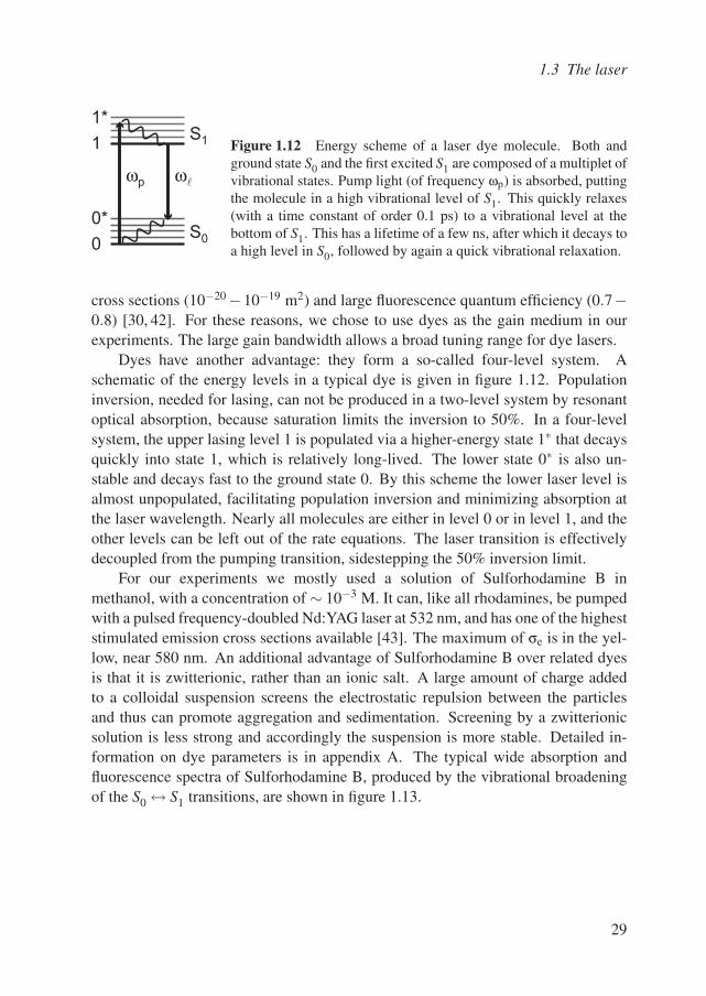
Figure 1.12 Energy scheme of a laser dye molecule. Both andground state S0 and the first excited S1 are composed of a multiplet ofvibrational states. Pump light (of frequency ωp) is absorbed, puttingthe molecule in a high vibrational level of S1. This quickly relaxes(with a time constant of order 0.1 ps) to a vibrational level at thebottom of S1. This has a lifetime of a few ns, after which it decays toa high level in S0, followed by again a quick vibrational relaxation.
cross sections (10−20 −10−19 m2) and large fluorescence quantum efficiency (0.7−0.8) [30, 42]. For these reasons, we chose to use dyes as the gain medium in ourexperiments. The large gain bandwidth allows a broad tuning range for dye lasers.
Dyes have another advantage: they form a so-called four-level system. Aschematic of the energy levels in a typical dye is given in figure 1.12. Populationinversion, needed for lasing, can not be produced in a two-level system by resonantoptical absorption, because saturation limits the inversion to 50%. In a four-levelsystem, the upper lasing level 1 is populated via a higher-energy state 1∗ that decaysquickly into state 1, which is relatively long-lived. The lower state 0∗ is also un-stable and decays fast to the ground state 0. By this scheme the lower laser level isalmost unpopulated, facilitating population inversion and minimizing absorption atthe laser wavelength. Nearly all molecules are either in level 0 or in level 1, and theother levels can be left out of the rate equations. The laser transition is effectivelydecoupled from the pumping transition, sidestepping the 50% inversion limit.
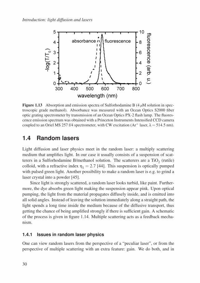
For our experiments we mostly used a solution of Sulforhodamine B inmethanol, with a concentration of ∼ 10−3 M. It can, like all rhodamines, be pumpedwith a pulsed frequency-doubled Nd:YAG laser at 532 nm, and has one of the higheststimulated emission cross sections available [43]. The maximum of σe is in the yel-low, near 580 nm. An additional advantage of Sulforhodamine B over related dyesis that it is zwitterionic, rather than an ionic salt. A large amount of charge addedto a colloidal suspension screens the electrostatic repulsion between the particlesand thus can promote aggregation and sedimentation. Screening by a zwitterionicsolution is less strong and accordingly the suspension is more stable. Detailed in-formation on dye parameters is in appendix A. The typical wide absorption andfluorescence spectra of Sulforhodamine B, produced by the vibrational broadeningof the S0 ↔ S1 transitions, are shown in figure 1.13.
29
Introduction: light diffusion and lasers
300 400 500 600 700 800
0
1
2
3
4
5
fluorescenceabsorbance
-log(T/T
0 )
wavelength (nm)
0
2
4
6
8
10 fluore
scence (a
rb. u
.)
Figure 1.13 Absorption and emission spectra of Sulforhodamine B (4 µM solution in spec-troscopic grade methanol). Absorbance was measured with an Ocean Optics S2000 fiberoptic grating spectrometer by transmission of an Ocean Optics PX-2 flash lamp. The fluores-cence emission spectrum was obtained with a Princeton Instruments Intensified CCD cameracoupled to an Oriel MS 257 f/4 spectrometer, with CW excitation (Ar+ laser, λ = 514.5 nm).
1.4 Random lasers
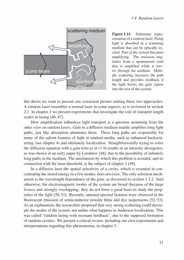
Light diffusion and laser physics meet in the random laser: a multiply scatteringmedium that amplifies light. In our case it usually consists of a suspension of scat-terers in a Sulforhodamine B/methanol solution. The scatterers are a TiO2 (rutile)colloid, with a refractive index η1 = 2.7 [44]. This suspension is optically pumpedwith pulsed green light. Another possibility to make a random laser is e.g. to grind alaser crystal into a powder [45].
Since light is strongly scattered, a random laser looks turbid, like paint. Further-more, the dye absorbs green light making the suspension appear pink. Upon opticalpumping, the light from the material propagates diffusely inside, and is emitted intoall solid angles. Instead of leaving the solution immediately along a straight path, thelight spends a long time inside the medium because of the diffusive transport, thusgetting the chance of being amplified strongly if there is sufficient gain. A schematicof the process is given in figure 1.14. Multiple scattering acts as a feedback mecha-nism.
1.4.1 Issues in random laser physics
One can view random lasers from the perspective of a “peculiar laser”, or from theperspective of multiple scattering with an extra feature: gain. We do both, and in
30
1.4 Random lasers
pump beam
scattering medium
amplifying
spontaneous
seed
Figure 1.14 Schematic repre-sentation of a random laser. Pumplight is absorbed in a scatteringmedium that can be optically ex-cited. Part of the system becomesamplifying. The emission orig-inates from a spontaneous seedthat is amplified while it trav-els through the medium. Multi-ple scattering increases the pathlength and provides feedback ifthe light leaves the gain regioninto the rest of the system.
this thesis we want to present one consistent picture uniting those two approaches.A random laser resembles a normal laser in some aspects, as is reviewed in section2.1. In chapter 2 we present experiments that investigate the role of transport lengthscales in lasing [46, 47].
How amplification influences light transport is a question stemming from theother view on random lasers. Gain in a diffusive medium mainly amplifies long lightpaths, just like absorption attenuates them. These long paths are responsible formany of the salient features of light in random media, such as enhanced backscat-tering (see chapter 4) and ultimately localization. Straightforwardly trying to solvethe diffusion equation with a gain term as in (1.9) results in an intensity divergence,as was shown in an early paper by Letokhov [48], due to the possibility of infinitelylong paths in the medium. The mechanism by which this problem is avoided, and itsconnection with the laser threshold, is the subject of chapter 3 [49].
In a diffusive laser the spatial selectivity of a cavity, which is essential in con-centrating the stored energy in a few modes, does not exist. The only selection mech-anism is the wavelength dependence of the gain, as discussed in section 1.3.2. Saidotherwise, the electromagnetic modes of the system are broad (because of the largelosses) and strongly overlapping; they do not form a good basis to study the prop-erties of the light [50, 51]. Recently, unusual spectral features were observed in thefluorescent emission of semiconductor powder films and dye suspensions [52, 53].As an explanation, the researchers proposed that very strong scattering could decou-ple the modes of the system, not unlike what happens in Anderson localization. Thiswas called “random lasing with resonant feedback”, due to the supposed formationof random cavities. We present a critical review, including our own experiments andinterpretations regarding this phenomenon, in chapter 5.
31
Introduction: light diffusion and lasers
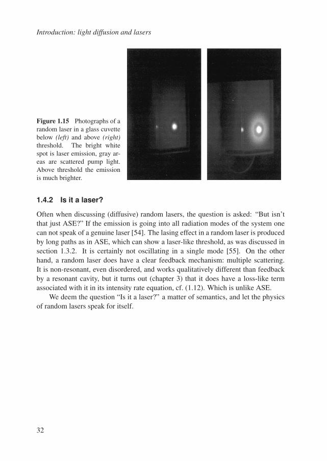
Figure 1.15 Photographs of arandom laser in a glass cuvettebelow (left) and above (right)threshold. The bright whitespot is laser emission, gray ar-eas are scattered pump light.Above threshold the emissionis much brighter.
1.4.2 Is it a laser?
Often when discussing (diffusive) random lasers, the question is asked: “But isn’tthat just ASE?” If the emission is going into all radiation modes of the system onecan not speak of a genuine laser [54]. The lasing effect in a random laser is producedby long paths as in ASE, which can show a laser-like threshold, as was discussed insection 1.3.2. It is certainly not oscillating in a single mode [55]. On the otherhand, a random laser does have a clear feedback mechanism: multiple scattering.It is non-resonant, even disordered, and works qualitatively different than feedbackby a resonant cavity, but it turns out (chapter 3) that it does have a loss-like termassociated with it in its intensity rate equation, cf. (1.12). Which is unlike ASE.
We deem the question “Is it a laser?” a matter of semantics, and let the physicsof random lasers speak for itself.
32
2.Amplifying volume in
scattering media
We investigate the influence of the excitation spot diameter on the laser thresholdof a scattering amplifying medium. Fluorescence spectra are recorded from a sus-pension of dielectric scatterers in a laser dye. The threshold pump fluence is foundto increase by a factor 70 if the excitation beam diameter becomes comparable tothe mean free path . This increase is explained using a simple model describingdiffusion out of the amplifying volume, and confirmed by a Monte Carlo simulation.
The output characteristics of a random laser show a threshold as a function of theexcitation power, or pump rate. This in itself is a remarkable observation, and oneof the central themes of this work is to investigate why this nonlinear dependenceexists and what determines its properties. As was discussed in the previous chapter,the threshold in an ordinary laser is the pump rate where the supplied amount ofenergy to the system is large enough to establish a gain that overcomes the loss inthe lasing mode. In a random laser, light propagates diffusively and a clear lasingmode can not be identified. Still, the threshold is there to be explained, and a clueis that it does not exist in systems without multiple scattering, as will be shown laterin this chapter. Apparently, diffusive transport plays a role in the threshold and thatmeans that the characteristic length scale for transport should have an influence.
As a short introduction to known results and for later reference, a concise sur-vey of observations surrounding the random laser threshold is given in section 2.1,followed by a qualitative discussion of the physical mechanisms giving rise to thesephenomena in 2.2. After this introduction, we will discuss the experiments and simu-lations that demonstrate the importance of the transport length for light amplificationin a random medium. A remark about units: in the following discussion, and in theother chapters describing experiments, the pump energy supply will be quantifiedin units of energy/area representing a fluence, typically of the order µJ/mm2. The
33
Amplifying volume in scattering media
580 600 6200.0
0.2
0.4
0.6
0.8
1.0(a)
C
B
A
norm
aliz
ed inte
nsity
wavelength (nm)
10-4
10-3
10-2
10-1
100
0
10
20
30
40
50(b)
FW
HM
(nm
)
Ip (mJ mm
-2)
threshold
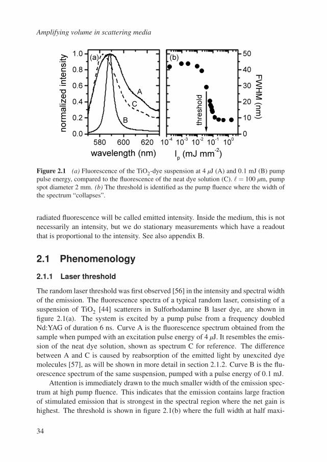
Figure 2.1 (a) Fluorescence of the TiO2-dye suspension at 4 µJ (A) and 0.1 mJ (B) pumppulse energy, compared to the fluorescence of the neat dye solution (C). = 100 µm, pumpspot diameter 2 mm. (b) The threshold is identified as the pump fluence where the width ofthe spectrum “collapses”.
radiated fluorescence will be called emitted intensity. Inside the medium, this is notnecessarily an intensity, but we do stationary measurements which have a readoutthat is proportional to the intensity. See also appendix B.
2.1 Phenomenology
2.1.1 Laser threshold
The random laser threshold was first observed [56] in the intensity and spectral widthof the emission. The fluorescence spectra of a typical random laser, consisting of asuspension of TiO2 [44] scatterers in Sulforhodamine B laser dye, are shown infigure 2.1(a). The system is excited by a pump pulse from a frequency doubledNd:YAG of duration 6 ns. Curve A is the fluorescence spectrum obtained from thesample when pumped with an excitation pulse energy of 4 µJ. It resembles the emis-sion of the neat dye solution, shown as spectrum C for reference. The differencebetween A and C is caused by reabsorption of the emitted light by unexcited dyemolecules [57], as will be shown in more detail in section 2.1.2. Curve B is the flu-orescence spectrum of the same suspension, pumped with a pulse energy of 0.1 mJ.
Attention is immediately drawn to the much smaller width of the emission spec-trum at high pump fluence. This indicates that the emission contains large fractionof stimulated emission that is strongest in the spectral region where the net gain ishighest. The threshold is shown in figure 2.1(b) where the full width at half maxi-
34
2.1 Phenomenology
0.00 0.05 0.10 0.15
0
2
4
6
8
10
12
14
outp
ut energ
y (J)
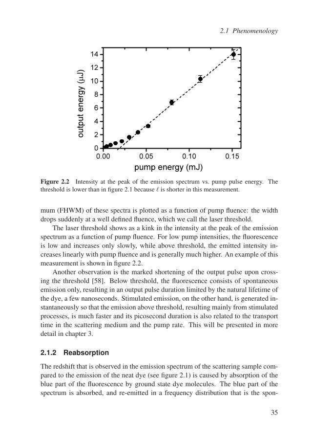
pump energy (mJ)
Figure 2.2 Intensity at the peak of the emission spectrum vs. pump pulse energy. Thethreshold is lower than in figure 2.1 because is shorter in this measurement.
mum (FHWM) of these spectra is plotted as a function of pump fluence: the widthdrops suddenly at a well defined fluence, which we call the laser threshold.
The laser threshold shows as a kink in the intensity at the peak of the emissionspectrum as a function of pump fluence. For low pump intensities, the fluorescenceis low and increases only slowly, while above threshold, the emitted intensity in-creases linearly with pump fluence and is generally much higher. An example of thismeasurement is shown in figure 2.2.
Another observation is the marked shortening of the output pulse upon cross-ing the threshold [58]. Below threshold, the fluorescence consists of spontaneousemission only, resulting in an output pulse duration limited by the natural lifetime ofthe dye, a few nanoseconds. Stimulated emission, on the other hand, is generated in-stantaneously so that the emission above threshold, resulting mainly from stimulatedprocesses, is much faster and its picosecond duration is also related to the transporttime in the scattering medium and the pump rate. This will be presented in moredetail in chapter 3.
2.1.2 Reabsorption
The redshift that is observed in the emission spectrum of the scattering sample com-pared to the emission of the neat dye (see figure 2.1) is caused by absorption of theblue part of the fluorescence by ground state dye molecules. The blue part of thespectrum is absorbed, and re-emitted in a frequency distribution that is the spon-
35
Amplifying volume in scattering media
580 600 6200.0
0.2
0.4
0.6
0.8
1.0
1.2(a) mm from
center
2.0
1.5
1.0
0.5
0
norm
. in
tensity
wavelength (nm)0 2 4
580
590
600
610(b)
peak w
avele
ngth
(nm
)
dist. from
center (mm)
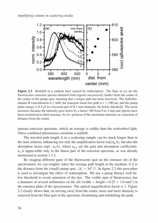
Figure 2.3 Redshift in a random laser caused by reabsorption. The lines in (a) are thefluorescence emission spectra obtained from regions successively farther from the center ofthe center of the pump spot, meaning that a longer path has been traversed. The Sulforho-damine B concentration is 1 mM, the transport mean free path is = 100 µm, and the pumppulse energy is 0.5 µJ in a focused spot of 0.1 mm diameter, far below threshold. The noiseincreases because the intensity goes down by a factor 100 from 0 to 2 mm and spectra havebeen normalized to their maxima. In (b): position of the maximum intensity as a function ofdistance from the center.
taneous emission spectrum, which on average is redder than the reabsorbed light.These combined phenomena constitute a redshift.
The traveled path length Λ in a scattering sample can be much longer than inthe neat solution, enhancing not only the amplification factor exp(κgΛ), but also theabsorption factor exp(−κaΛ), where κg,a are the gain and absorption coefficients.κa is appreciable only in the bluest part of the emission spectrum, as was alreadymentioned in section 1.3.3.
By imaging different parts of the fluorescent spot on the entrance slit of thespectrometer we can roughly select the average path length in the medium: if d isthe distance from the (small) pump spot, 〈Λ〉 = 3d2/. In figure 2.3 this procedureis used to investigate the effect of reabsorption. We use a pump fluence well be-low threshold to avoid saturation of the dye. The visible spot of fluorescence hasa diameter of several millimeters on the slit (width × height = 0.25 × 1.0 mm2) inthe entrance plate of the spectrometer. The optical magnification factor is 1. Figure2.3 clearly shows that, on moving away from the center, more and more intensity isremoved from the blue part of the spectrum, broadening and redshifting the peak.
36
2.2 Qualitative explanation of the random laser threshold
2.2 Qualitative explanation of the random laserthreshold
In this section these observations will be used to compose a qualitative picture ofthe threshold. The spectral narrowing is intimately connected to the threshold asmeasured in the emitted peak intensity; actually they are one phenomenon [59].
As was discussed in section 1.3, the threshold of a laser depends on the balancebetween gain and loss of light in the system. The total amount of amplification de-pends on the product κgΛ, counting only the path length traveled in the amplifyingmedium. In a random laser the feedback mechanism is multiple scattering. Incom-plete feedback is a loss factor. Accordingly, the loss and the distribution of traveledpath lengths originate from the same mechanism: diffusion of light. If we now as-sume that the transport parameters do not depend strongly on the wavelength of thelight (most random lasers consist of polydisperse, nonspherical scatterers, washingout the fine wavelength structure in the scattering properties of the material) then allspectral features of the emission must be due to the wavelength dependence of thegain. For demonstration purposes we use the small signal gain limit to describe theintensity in a certain path: exp[κg(λ)Λ]. Light with wavelengths near the maximumof the gain is amplified more, receiving a larger spectral weight. This is the gainnarrowing mentioned in section 1.3.2.
Evidently, this mechanism does not cause more light to be emitted by the systemabove threshold, it is just spectrally redistributed. The wavelength variation of thegain of the amplifying medium is the only selection mechanism in a random laserthat distinguishes “laser” light from spontaneous emission. This means that the sharpbend at the laser threshold in the curve of emitted intensity vs. pump power is onlyobserved in the frequency range near the maximum, and should not be present in thespectrally integrated intensity.
In a conventional laser, the threshold can be observed in the total output intensityof the laser mode, because there is an additional selection mechanism for lasing thatis often much more restrictive than the spectral dependence of the gain: the modeprofile of the cavity. Only light radiated in the “right” solid angle, i.e. subtendedby the lasing mode, contributes, and the dominance of stimulated transitions abovethe laser threshold causes the abrupt change in behavior. If the radiation from aconventional laser would be collected in all directions, the threshold kink woulddisappear, because all the radiation, stimulated (laser) and spontaneous (non-laser),light is detected, analogous to a measurement of spectrally integrated emission froma random laser. We will revisit this analogy in the discussion of the β-factor of arandom laser in 3.3.
37
Amplifying volume in scattering media
Figure 2.4 Schematic of the exper-imental situation. The lens is movedto change the size of the pump spot.
samplepump beam
1 cm
l = 100 µm
100 µm
spot size
2 mm
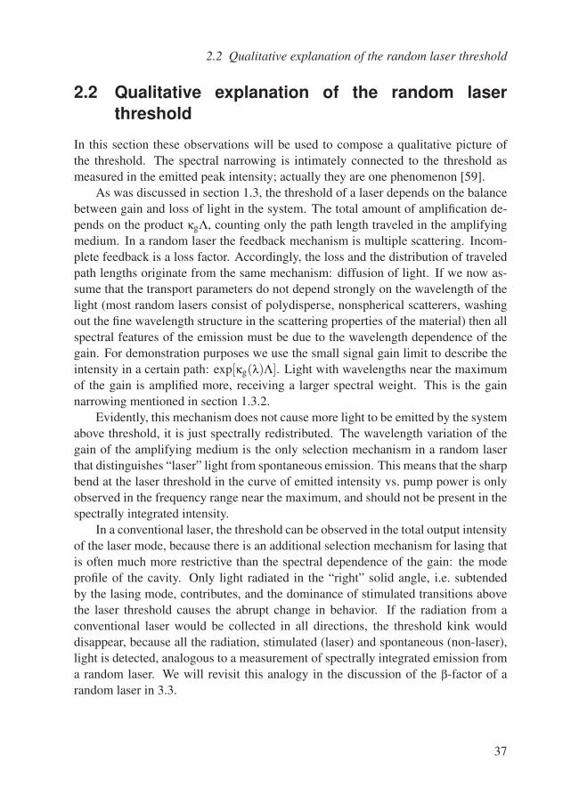
2.3 Amplifying volume in scattering media
In this section, we present experiments which demonstrate that the threshold of thesystem depends on the size of the pumped volume. The spatial distribution of gainis governed by the spreading of pump light in the system. The path length involvedin the amplification process is the length of diffusive paths through the gain volume.The gain volume is cylindrical; the diameter is set by the diameter of the excitationspot. The thickness d is related to the diffuse absorption length La =
√a/3. In
the absence of saturation, d = La, otherwise (as in this study) d > La. Due to mul-tiple scattering, the loss as well as the amplified path lengths, and hence the lasingthreshold, depend on the gain volume [60].
2.3.1 Experimental method
We record fluorescence spectra from a TiO2-dye [44] suspension as a function ofexcitation spot diameter and pump pulse energy. The scatterers are suspended in1.0 mM Sulforhodamine B dye dissolved in methanol. The TiO2 volume fraction is10−3, resulting in a transport mean free path = 100 ± 20 µm. is obtained fromcoherent backscattering, measured without the pump beam. The inelastic lengthof the dye solution is a = 110 µm. The thickness of the sample cell is L = 1 cm.During the experiments the suspension is stirred continuously to avoid sedimentationand dye degradation.
The pump source is a Spectra Physics DCR-2A frequency-doubled Q-switchedNd:YAG laser, giving 9 mJ pulses with a pulse duration of τp = 6 ns at a repetitionrate of 20 Hz, with a wavelength of 532 nm. The pulses are attenuated using a pair ofGlan prisms, of which one can be rotated to vary the pump pulse energy between 0
38
2.3 Amplifying volume in scattering media
10-4
10-3
10-2
10-1
100
101
0
10
20
30
40
50
d = 2 mm
d = 80 m
Ip (mJ mm
-2)
FW
HM
(nm
)
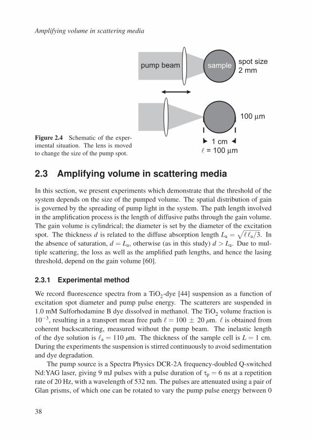
Figure 2.5 Linewidth vs. pump fluence for 2 mm (•) and 80 µm () pump diameters. Thelines are fits to the data. The threshold, indicated by the arrow, depends on spot size.
and 9 mJ. The pump beam is incident on the sample through a lens ( f = 6 cm), whichis on a translation stage. By moving the lens along the pump beam the diameter(beam waist at 1/e2) of the spot on the sample cell is varied between 80 µm (inthe focus) and 2 mm. The excitation and detection directions are at an angle of ≈20. The fluorescence is focused on the entrance slit of a Spex 1672 Czerny-Turnertype f = 250 mm spectrometer, used in single stage configuration. The spectrum isrecorded with a Princeton Instruments 1412 diode array (1024 pixels × 14 bits).
In figure 2.5 the full width at half maximum (FWHM) of the spectra is plottedas a function of the pump fluence. From these data we define the laser thresholdas the inflection point of a sigmoidal fit through the data points. This procedure isrepeated for a number of different excitation spot sizes. On decreasing the pumpbeam diameter, the threshold intensity shifts to values that are 70 times higher thanthose measured with the largest spot sizes. There is a difference in FWHM belowthreshold for the two curves shown in figure 2.5, due to a difference in spectralshape which is caused by reabsorption. The change of FWHM within one seriescan however be reliably used to determine the threshold. The diameter of the pumpbeam strongly influences the threshold intensity, as is evident from figure 2.6. Aconsequence of this result is that an experiment on random lasers will yield differentresults depending on whether a focused pump beam or a plane wave excitation isused. Note that we vary the beam size independently of . In earlier work [56, 58] was varied and (occasionally) > L, so necessarily also > pump beam size. A
39
Amplifying volume in scattering media
0 5 10 15 20
0.1
1
pump beam diameter (units )
thre
shold
Ip (
mJ m
m-2)
70 x
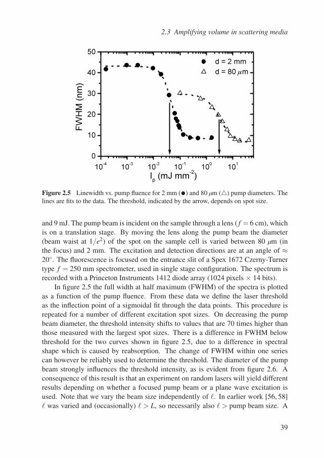
Figure 2.6 The threshold excitation intensity vs. pump beam diameter in units = 100 µm.At small pump spots, the threshold pump fluence increases by a factor 70 with respect to thethreshold large pump diameter.
change in properties of the system must then be attributed to the strongly differingtransport in the diffusive ( L) and single-scattering regimes. For comparison, theweakly scattering regime will be discussed in 2.3.2.
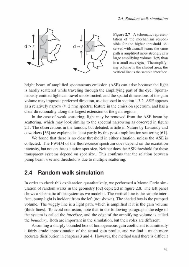
The increase of the threshold for small excitation regions is explained in thefollowing way (figure 2.7). Light is emitted in the pumped region of the sample,from where it starts to diffuse. If the pumped area is large, the amplifying volumeis large. Light that is emitted in the pumped volume can travel a long path insidethe part of the system that has gain: it is amplified strongly. If a path reaches thepassive (unexcited) part of the system, there is a large probability that it will returnto the amplifying region because of the large pumped area. For a small excitationbeam diameter, the light paths will very probably leave the amplifying region after ashort time, with a small chance to return. This means that a larger gain is needed tocompensate losses, i.e. the threshold is higher.
2.3.2 Weakly scattering medium
We asserted earlier that a change in the threshold pump intensity due to a change inexcitation spot size would be an effect of multiple scattering. In order to verify thisclaim, we repeated the experiment on a neat dye solution and on a suspension with ≈ 2 cm (> L).
In a dye solution that is only weakly scattering or even not scattering at all, a
40
2.4 Random walk simulation
d > l d ≈ l
Figure 2.7 A schematic represen-tation of the mechanism respon-sible for the higher threshold ob-served with a small beam: the samepath is amplified more strongly in alarge amplifying volume (left) thanin a small one (right). The amplify-ing volume is the shaded area, thevertical line is the sample interface.
bright beam of amplified spontaneous emission (ASE) can arise because the lightis hardly scattered while traveling through the amplifying part of the dye. Sponta-neously emitted light can travel unobstructed, and the spatial dimensions of the gainvolume may impose a preferred direction, as discussed in section 1.3.2. ASE appearsas a relatively narrow (≈ 2 nm) spectral feature in the emission spectrum, and has aclear directionality along the largest extension of the gain region.
In the case of weak scattering, light may be removed from the ASE beam byscattering, which may look similar to the spectral narrowing as observed in figure2.1. The observations in the famous, but debated, article in Nature by Lawandy andcoworkers [56] are explained at least partly by this post-amplification scattering [61].
We found that there is no clear threshold in either situation, unless the ASE iscollected. The FWHM of the fluorescence spectrum does depend on the excitationintensity, but not on the excitation spot size. Neither does the ASE threshold for thesetransparent systems depend on spot size. This confirms that the relation betweenpump beam size and threshold is due to multiple scattering.
2.4 Random walk simulation
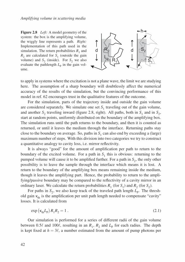
In order to check this explanation quantitatively, we performed a Monte Carlo sim-ulation of random walks in the geometry [62] depicted in figure 2.8. The left panelshows a schematic of the system as we model it. The vertical line is the sample inter-face, pump light is incident from the left (not shown). The shaded box is the pumpedvolume. The wiggly line is a light path, which is amplified if it is the gain volume(thick lines). To avoid confusion, note that in the following paragraphs the edge ofthe system is called the interface, and the edge of the amplifying volume is calledthe boundary. Both are important in the simulation, but their roles are different.
Assuming a sharply bounded box of homogeneous gain coefficient is admittedlya fairly crude approximation of the actual gain profile, and we find a much moreaccurate distribution in chapters 3 and 4. However, the method used there is difficult
41
Amplifying volume in scattering media
Figure 2.8 Left: A model geometry of thesystem: the box is the amplifying volume,the wiggly line represents a path. Right:Implementation of this path used in thesimulation. The return probabilities R1 andR2 are calculated for S1 (outside the gainvolume) and S2 (inside). For S2 we alsoevaluate the pathlength Lp in the gain vol-ume.
d dR2
Lp R1
S2
S1
h
to apply in systems where the excitation is not a plane wave, the limit we are studyinghere. The assumption of a sharp boundary will doubtlessly affect the numericalaccuracy of the results of the simulation, but the convincing performance of thismodel in ref. 62 encourages trust in the qualitative features of the outcome.
For the simulation, parts of the trajectory inside and outside the gain volumeare considered separately. We simulate one set S1 traveling out of the gain volume,and another S2 traveling inward (figure 2.8, right). All paths, both in S1 and in S2,start at random points, uniformly distributed on the boundary of the amplifying box.The simulation runs until the path returns to the boundary, and then it is counted asreturned, or until it leaves the medium through the interface. Returning paths stayclose to the boundary on average. So, paths in S1 can also end by exceeding a (large)maximum number of steps. With this division into two categories we try to constructa quantitative analogy to cavity loss, i.e. mirror reflectivity.
It is always “good” for the amount of amplification per path to return to theboundary of the excited volume. For a path in S1 this is obvious: returning to thepumped volume will cause it to be amplified further. For a path in S2, the only otherpossibility is to leave the sample through the interface which means it is lost. Areturn to the boundary of the amplifying box means remaining inside the medium,though it leaves the amplifying part. Hence, the probability to return to the ampli-fying/passive boundary may be compared to the reflectivity of a cavity mirror in anordinary laser. We calculate the return probabilities R1 (for S1) and R2 (for S2).
For paths in S2, we also keep track of the traveled path length Lp. The thresh-old gain κth is the amplification per unit path length needed to compensate “cavity”losses. It is calculated from
exp(
κthLp)
R1R2 = 1 . (2.1)
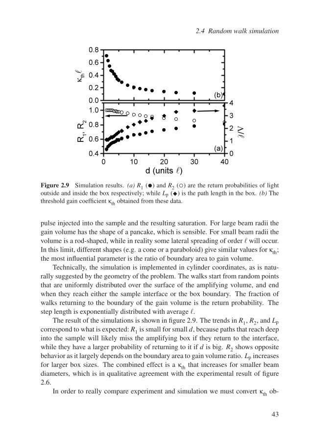
Our simulation is performed for a series of different radii of the gain volumebetween 0.5 and 100, resulting in an R1, R2 and Lp for each radius. The depthis kept fixed at h = 3, a number estimated from the amount of pump photons per
42
2.4 Random walk simulation
0.0
0.2
0.4
0.6
0.8
(b)
th
0 10 20 30 400.4
0.6
0.8
1.0
R1,
R2
d (units )
0
1
2
3
4
(a)
/
Figure 2.9 Simulation results. (a) R1 (•) and R2 () are the return probabilities of lightoutside and inside the box respectively; while Lp ( ) is the path length in the box. (b) Thethreshold gain coefficient κth obtained from these data.
pulse injected into the sample and the resulting saturation. For large beam radii thegain volume has the shape of a pancake, which is sensible. For small beam radii thevolume is a rod-shaped, while in reality some lateral spreading of order will occur.In this limit, different shapes (e.g. a cone or a paraboloid) give similar values for κth;the most influential parameter is the ratio of boundary area to gain volume.
Technically, the simulation is implemented in cylinder coordinates, as is natu-rally suggested by the geometry of the problem. The walks start from random pointsthat are uniformly distributed over the surface of the amplifying volume, and endwhen they reach either the sample interface or the box boundary. The fraction ofwalks returning to the boundary of the gain volume is the return probability. Thestep length is exponentially distributed with average .
The result of the simulations is shown in figure 2.9. The trends in R1, R2, and Lp
correspond to what is expected: R1 is small for small d, because paths that reach deepinto the sample will likely miss the amplifying box if they return to the interface,while they have a larger probability of returning to it if d is big. R2 shows oppositebehavior as it largely depends on the boundary area to gain volume ratio. Lp increasesfor larger box sizes. The combined effect is a κth that increases for smaller beamdiameters, which is in qualitative agreement with the experimental result of figure2.6.
In order to really compare experiment and simulation we must convert κth ob-
43
Amplifying volume in scattering media
tained from R1, R2 and Lp to a threshold pump intensity. The method we use isadapted from refs. 63, 64 to explicitly include saturation effects: the threshold inver-sion is a substantial fraction of the total population.
The threshold gain is inserted in a set of laser rate equations where only cavitylosses are considered. We analyze the system in steady state for simplicity, corre-sponding to a CW situation. The pump pulse in our experiments is much longer thanthe time it takes for a quasi-steady state to develop. This time is of the order of 100ps, according to earlier simulations [60], and also according to chapter 3. On theother hand, the pump pulse is short enough to neglect population of the triplet stateof the dye [64] (buildup time in the order of 100 ns). Isolating the pump intensity Ip
in terms of κth results in the relation
Ip =ηhωp
σaτκth
κ0 −κth. (2.2)
Here κ0 is related to the maximum gain, and has a numeric value of κ0 = 77 cm−1 =0.77−1. η is the refractive index of the solution, hωp is the pump photon energy,σa is the absorption cross section of the dye for pump light, and τ is the excitedstate lifetime of the dye in methanol. Numerical values for the parameters of Sul-forhodamine B may be found in table A.1 on page 111. Because of the steady statecharacter of the analysis, the result is a pump intensity (incident power per area inW/m2), rather than the fluence (incident energy per area in J/m2). Intensity is con-verted into fluence with the help of the pulse duration τp. The final result is shownin figure 2.10.
2.5 Discussion
Comparing the results from experiment and simulation, we see that there is an ex-cellent agreement in the behavior of the threshold pump intensity as a function ofthe excitation spot diameter. The upturn at small diameters that is observed in theexperiment is correctly reproduced by the simulation. The dependence of the thresh-old intensity is well explained by the model described above. Intensities from theexperiment are a factor ≈ 2 larger than those from the calculation; the difference islargely caused by two relevant processes that are not included of our model.
The most important aspect is that we assume all incident pump light is absorbed.Because of the method of simulation we chose, i.e. we only simulate propagatingemitted light and not the incident pump light, it is not possible to extract the amountof absorbed pump light. However, since the inelastic length a is about equal to thetransport length , we expect approximately half of the pump light to be scatteredout of the system within the first absorption length. This effect would just cancel
44
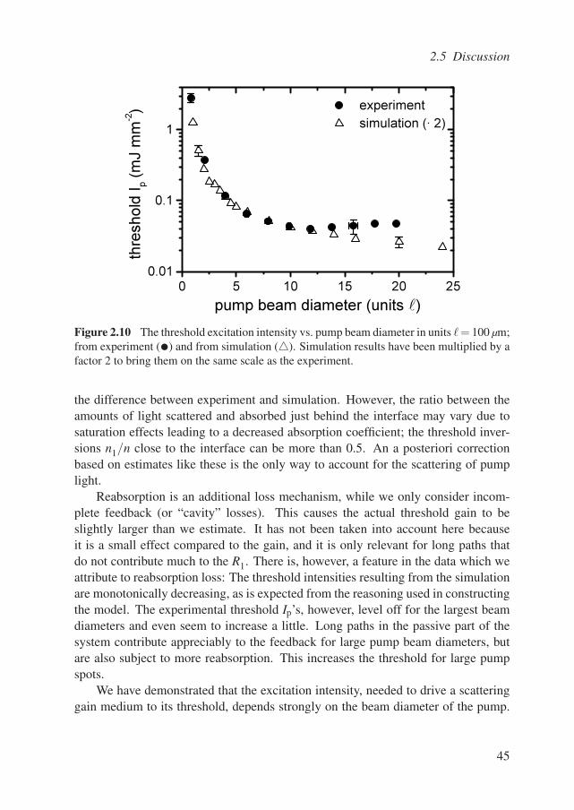
2.5 Discussion
0 5 10 15 20 250.01
0.1
1
experiment
simulation (· 2)
pump beam diameter (units )
thre
shold
Ip (
mJ m
m-2)
Figure 2.10 The threshold excitation intensity vs. pump beam diameter in units = 100 µm;from experiment (•) and from simulation (). Simulation results have been multiplied by afactor 2 to bring them on the same scale as the experiment.
the difference between experiment and simulation. However, the ratio between theamounts of light scattered and absorbed just behind the interface may vary due tosaturation effects leading to a decreased absorption coefficient; the threshold inver-sions n1/n close to the interface can be more than 0.5. An a posteriori correctionbased on estimates like these is the only way to account for the scattering of pumplight.
Reabsorption is an additional loss mechanism, while we only consider incom-plete feedback (or “cavity” losses). This causes the actual threshold gain to beslightly larger than we estimate. It has not been taken into account here becauseit is a small effect compared to the gain, and it is only relevant for long paths thatdo not contribute much to the R1. There is, however, a feature in the data which weattribute to reabsorption loss: The threshold intensities resulting from the simulationare monotonically decreasing, as is expected from the reasoning used in constructingthe model. The experimental threshold Ip’s, however, level off for the largest beamdiameters and even seem to increase a little. Long paths in the passive part of thesystem contribute appreciably to the feedback for large pump beam diameters, butare also subject to more reabsorption. This increases the threshold for large pumpspots.
We have demonstrated that the excitation intensity, needed to drive a scatteringgain medium to its threshold, depends strongly on the beam diameter of the pump.
45
Amplifying volume in scattering media
This effect is due to multiple scattering: it is not observed in the absence of scatterers.Light that propagates diffusively through the medium starts from the excited volumeand is amplified less strongly if the amplifying region of the sample has a smalldiameter, in the order of 5, giving rise to a threshold that is up to 70 times higherthan if the gain volume is large. The experimental data are accurately reproduced bya Monte Carlo random walk simulation.
46
3.Dynamics of the
threshold crossing
Amplification influences light transport in disordered systems. In this chapter wepresent and interpret detailed calculations of diffusion in a saturable medium thatabsorbs green light and amplifies red light. The propagation of both pump andlaser light are taken into account, coupled to a rate equation for the populationinversion. We identify the diffusive analogue of loss in these generalized laserequations, and investigate the threshold crossing. The full dynamics of the interplaybetween field and population is found to be an essential part of a description of arandom laser close to or above the laser threshold. The full transport equationsare not very transparent at first sight due to their nonlinearity, and can only besolved numerically. To prevent a “black box” presentation, we start by discussingsimplifications and approximations of the complete formalism to demonstrate thephysics.
Light is amplified according to the exponential relation eκgΛ, where κg is the gaincoefficient and Λ is the path length traveled in the amplifying medium. This rela-tion was already discussed as Beer’s law (1.3), and here we use it with a negativeabsorption coefficient. It immediately reveals the difference in the effect of gain onlong and short paths: with a constant κg, the paths of large Λ are amplified muchmore strongly. The transport characteristics of light change strongly in the presenceof gain, as will be discussed below in section 3.1.
The most straightforward way of incorporating gain in multiple scattering is byinclusion of a gain term in the diffusion equation, as in (1.9):
∂W∂ t
= D∇2W +κgcW +S . (3.1)
47
Dynamics of the threshold crossing
3.1 The photon bomb
Solutions of (3.1) turn out to exist only for a finite sized systems [48]. The maximumvolume for which a solution can be found is called the critical volume Vcr. Thephysical background for this behavior is the possibility of infinitely long paths indiffusion, which will be amplified to infinite intensities in a gain medium. The resultis a diverging intensity, occurring whenever the probability for a path to be scatteredout of the system is compensated by the gain. Chances of leaving the medium aresmaller for larger systems, so the smaller the gain the larger Vcr. Because of thesimilarity with neutron diffusion in fissionable material, exploding at the criticalvolume, the critical random laser is also called the “photon bomb”.
Solutions of (3.1) are found by a method analogous to solving the time depen-dent Schrodinger equation: first we find the eigenfunctions φn(r) and eigenvalues εn
of the stationary part. These have the simple time-evolution φn(r, t) = φn(r,0)e−Dεnt .Then W (r, t) = ∑n anφn(r, t), where the an are determined by W (r,0). The exponen-tial time dependence shows that the eigenfunction with the smallest eigenvalue soondominates the entire sum, and that as soon as there is an εn < 0, the intensity growswith time. This is called the generation threshold.
The stationary part of (3.1) is solved for a slab that is finite only in the z-directionwith thickness L:
−[
∂ 2
∂ z2 +3κg
]φn = εnφn , (3.2)
which is like a particle-in-a-box problem with the bottom of the box at a potential−3κg/. The boundary conditions are in principle [20] (1.10), but for demonstrationpurposes we allow ourselves the small error of just extrapolating φn to zero a distanceze outside the slab. The φn are then of the form
φn(z) ∝ sinknz with kn ≡√
εn +3κg
=
nπZ
. (3.3)
Here Z = L+2ze. The lowest eigenvalue ε1 reaches zero at Z = π√
/(3κg), and thecritical thickness Lcr = πLg, if L ze and Lg =
√g/3 is the diffusive gain length,
similar to the diffusive absorption length (1.11).
Connection with the laser threshold The intensity in an actual random laser willof course not diverge, ultimately by energy conservation. The question is what hap-pens instead. The intensity divergence has severely hampered theoretical effortsfor systems beyond the critical point, L > Lcr. The divergence has been identifiedwith the laser threshold in several theoretical papers [65–70], although none of them
48
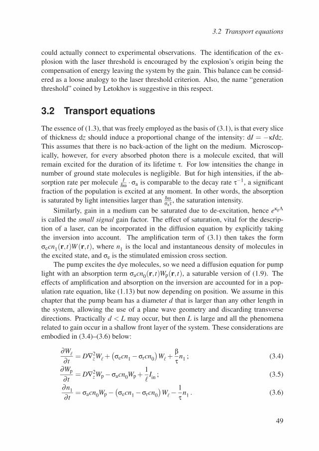
3.2 Transport equations
could actually connect to experimental observations. The identification of the ex-plosion with the laser threshold is encouraged by the explosion’s origin being thecompensation of energy leaving the system by the gain. This balance can be consid-ered as a loose analogy to the laser threshold criterion. Also, the name “generationthreshold” coined by Letokhov is suggestive in this respect.
3.2 Transport equations
The essence of (1.3), that was freely employed as the basis of (3.1), is that every sliceof thickness dz should induce a proportional change of the intensity: dI = −κIdz.This assumes that there is no back-action of the light on the medium. Microscop-ically, however, for every absorbed photon there is a molecule excited, that willremain excited for the duration of its lifetime τ. For low intensities the change innumber of ground state molecules is negligible. But for high intensities, if the ab-sorption rate per molecule I
hω ·σa is comparable to the decay rate τ−1, a significantfraction of the population is excited at any moment. In other words, the absorptionis saturated by light intensities larger than hω
σaτ , the saturation intensity.
Similarly, gain in a medium can be saturated due to de-excitation, hence eκgΛ
is called the small signal gain factor. The effect of saturation, vital for the descrip-tion of a laser, can be incorporated in the diffusion equation by explicitly takingthe inversion into account. The amplification term of (3.1) then takes the formσecn1(r, t)W (r, t), where n1 is the local and instantaneous density of molecules inthe excited state, and σe is the stimulated emission cross section.
The pump excites the dye molecules, so we need a diffusion equation for pumplight with an absorption term σacn0(r, t)Wp(r, t), a saturable version of (1.9). Theeffects of amplification and absorption on the inversion are accounted for in a pop-ulation rate equation, like (1.13) but now depending on position. We assume in thischapter that the pump beam has a diameter d that is larger than any other length inthe system, allowing the use of a plane wave geometry and discarding transversedirections. Practically d < L may occur, but then L is large and all the phenomenarelated to gain occur in a shallow front layer of the system. These considerations areembodied in (3.4)–(3.6) below:
∂W
∂ t= D∇2
zW +(
σecn1 −σrcn0
)W +
βτ
n1 ; (3.4)
∂Wp
∂ t= D∇2
zWp −σacn0Wp +1
Iin ; (3.5)
∂n1
∂ t= σacn0Wp −
(σecn1 −σrcn0
)W−
1τ
n1 . (3.6)
49
Dynamics of the threshold crossing
In these equations, W and Wp are the “laser” and pump light densities. We speakof laser light because only the light partaking in the amplification process is in (3.4),not all emitted luminescence. The ground state and excited state populations are n0and n1, satisfying n0 +n1 = n, the total dye concentration.
The spectral dependence is not in (3.4). The real molecular absorption andstimulated emission cross sections vary with wavelength, and so should be read asσe = σe(λ) and σa = σa(λp). The effect of reabsorption on the emission spectrumwas presented in section 2.1.2. In these wavelength-independent equations, reab-sorption is accounted for by an absorption term with a cross section σr = σa(λ).This cross section is small, typically a few percent of σe(λ) for laser dyes, but itseffect is appreciable because of the exponential attenuation of long light paths.
The source terms in (3.4) and (3.5) differ in physical origin. The pump lightstems from an incident beam, written here as −1Iin(z, t). It decays exponentiallywith z as a result of scattering and absorption. As a result, the pump mainly excitesthe dye in a layer with a thickness of order La near the pump face of the sample.The t-dependence of Iin is the pump pulse profile in time. The source of laser lightis the spontaneous emission term βn1τ−1, where τ is the natural lifetime and β is thespontaneous emission factor, see section 3.3.
The equations (3.4)–(3.6) completely determine the transport of pump and laserlight, coupled to the population dynamics, in a diffusive system. They form a set ofcoupled nonlinear partial differential equations, subject to the boundary conditions1.10, and need to be solved simultaneously. This is done by numerical integration,as will be described in section 3.4.2.
3.3 β-factor in a random laser
Spontaneous emission is usually the seed for lasing, both in cavity and in randomlasers. However, not all spontaneous emission participates in the laser process. Thefraction of spontaneous radiation that does contribute to lasing is called β, introducedin section 1.3.1.
Random lasers have been described until now without β [62, 71], yet the obser-vation of a nonzero threshold does clearly necessitate a β < 1. A reliable numericalvalue of β is indispensable for a model describing the response of a random laser toan applied pump pulse.
3.3.1 Spontaneous emission seeding in cavity and random lasers
In a cavity laser, light that is emitted outside a resonant mode of the cavity (outsidebeing either of the wrong direction or the wrong wavelength) does not stimulate
50
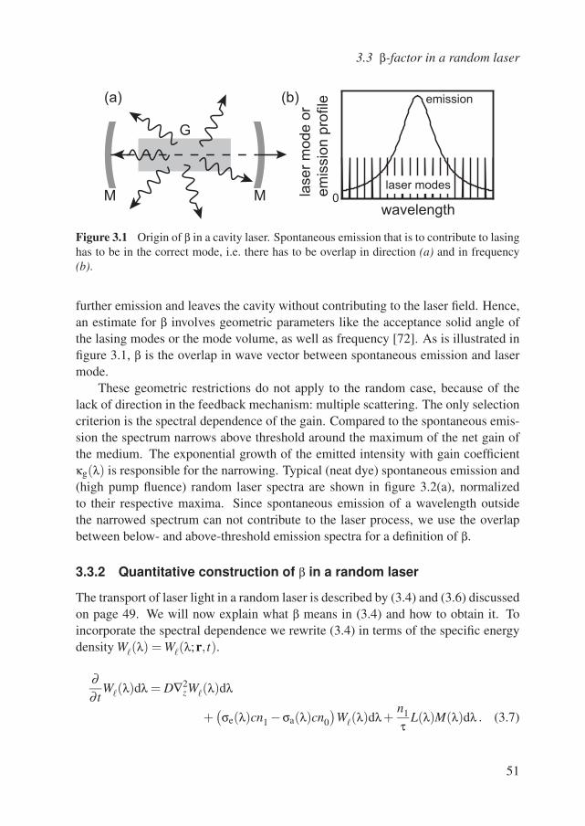
3.3 β-factor in a random laser
M
G
M 0laser modes
emission
wavelength
lase
r m
od
e o
r
em
issio
n p
rofile(a) (b)
Figure 3.1 Origin of β in a cavity laser. Spontaneous emission that is to contribute to lasinghas to be in the correct mode, i.e. there has to be overlap in direction (a) and in frequency(b).
further emission and leaves the cavity without contributing to the laser field. Hence,an estimate for β involves geometric parameters like the acceptance solid angle ofthe lasing modes or the mode volume, as well as frequency [72]. As is illustrated infigure 3.1, β is the overlap in wave vector between spontaneous emission and lasermode.
These geometric restrictions do not apply to the random case, because of thelack of direction in the feedback mechanism: multiple scattering. The only selectioncriterion is the spectral dependence of the gain. Compared to the spontaneous emis-sion the spectrum narrows above threshold around the maximum of the net gain ofthe medium. The exponential growth of the emitted intensity with gain coefficientκg(λ) is responsible for the narrowing. Typical (neat dye) spontaneous emission and(high pump fluence) random laser spectra are shown in figure 3.2(a), normalizedto their respective maxima. Since spontaneous emission of a wavelength outsidethe narrowed spectrum can not contribute to the laser process, we use the overlapbetween below- and above-threshold emission spectra for a definition of β.
3.3.2 Quantitative construction of β in a random laser
The transport of laser light in a random laser is described by (3.4) and (3.6) discussedon page 49. We will now explain what β means in (3.4) and how to obtain it. Toincorporate the spectral dependence we rewrite (3.4) in terms of the specific energydensity W(λ) = W(λ;r, t).
∂∂ t
W(λ)dλ = D∇2zW(λ)dλ
+(
σe(λ)cn1 −σa(λ)cn0
)W(λ)dλ +
n1
τL(λ)M(λ)dλ . (3.7)
51
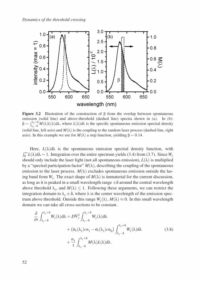
Dynamics of the threshold crossing
550 600 6500.0
0.2
0.4
0.6
0.8
1.0(a)
inte
nsity (
max =
1)
wavelength (nm)
550 600 6500.0
0.5
1.0
1.5
2.0
2.5
3.0(b)
L(
) /
10-2
0.0
0.2
0.4
0.6
0.8
1.0M()
Figure 3.2 Illustration of the construction of β from the overlap between spontaneousemission (solid line) and above-threshold (dashed line) spectra shown in (a). In (b):β =
∫ λ+δλ−δ
M(λ)L(λ)dλ, where L(λ)dλ is the specific spontaneous emission spectral density
(solid line, left axis) and M(λ) is the coupling to the random laser process (dashed line, rightaxis). In this example we use for M(λ) a step function, yielding β = 0.14.
Here, L(λ)dλ is the spontaneous emission spectral density function, with∫ ∞0 L(λ)dλ = 1. Integration over the entire spectrum yields (3.4) from (3.7). Since W
should only include the laser light (not all spontaneous emission), L(λ) is multipliedby a “spectral participation factor” M(λ), describing the coupling of the spontaneousemission to the laser process. M(λ) excludes spontaneous emission outside the las-ing band from W. The exact shape of M(λ) is immaterial for the current discussion,as long as it is peaked in a small wavelength range ±δ around the central wavelengthabove threshold λ, and M(λ) ≤ 1. Following these arguments, we can restrict theintegration domain to λ± δ, where λ is the center wavelength of the emission spec-trum above threshold. Outside this range W(λ), M(λ) ≈ 0. In this small wavelengthdomain we can take all cross-sections to be constant.
∂∂ t
∫ λ+δ
λ−δW(λ)dλ = D∇2
z
∫ λ+δ
λ−δW(λ)dλ
+(
σe(λ)cn1 −σr(λ)cn0
)∫ λ+δ
λ−δW(λ)dλ
+n1
τ
∫ λ+δ
λ−δM(λ)L(λ)dλ .
(3.8)
52
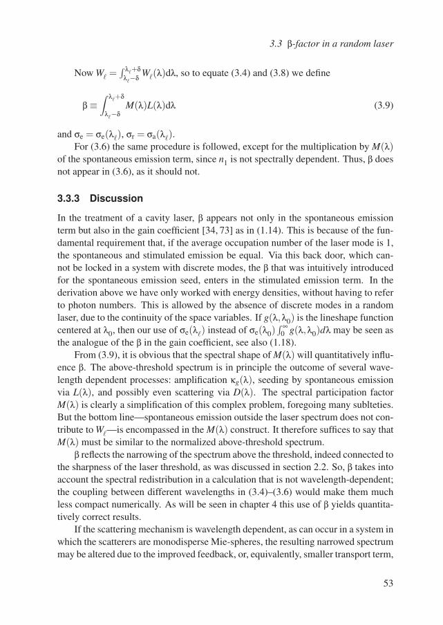
3.3 β-factor in a random laser
Now W =∫ λ+δ
λ−δ W(λ)dλ, so to equate (3.4) and (3.8) we define
β ≡∫ λ+δ
λ−δM(λ)L(λ)dλ (3.9)
and σe = σe(λ), σr = σa(λ).For (3.6) the same procedure is followed, except for the multiplication by M(λ)
of the spontaneous emission term, since n1 is not spectrally dependent. Thus, β doesnot appear in (3.6), as it should not.
3.3.3 Discussion
In the treatment of a cavity laser, β appears not only in the spontaneous emissionterm but also in the gain coefficient [34, 73] as in (1.14). This is because of the fun-damental requirement that, if the average occupation number of the laser mode is 1,the spontaneous and stimulated emission be equal. Via this back door, which can-not be locked in a system with discrete modes, the β that was intuitively introducedfor the spontaneous emission seed, enters in the stimulated emission term. In thederivation above we have only worked with energy densities, without having to referto photon numbers. This is allowed by the absence of discrete modes in a randomlaser, due to the continuity of the space variables. If g(λ,λ0) is the lineshape functioncentered at λ0, then our use of σe(λ) instead of σe(λ0)
∫ ∞0 g(λ,λ0)dλ may be seen as
the analogue of the β in the gain coefficient, see also (1.18).From (3.9), it is obvious that the spectral shape of M(λ) will quantitatively influ-
ence β. The above-threshold spectrum is in principle the outcome of several wave-length dependent processes: amplification κg(λ), seeding by spontaneous emissionvia L(λ), and possibly even scattering via D(λ). The spectral participation factorM(λ) is clearly a simplification of this complex problem, foregoing many sublteties.But the bottom line—spontaneous emission outside the laser spectrum does not con-tribute to W—is encompassed in the M(λ) construct. It therefore suffices to say thatM(λ) must be similar to the normalized above-threshold spectrum.
β reflects the narrowing of the spectrum above the threshold, indeed connected tothe sharpness of the laser threshold, as was discussed in section 2.2. So, β takes intoaccount the spectral redistribution in a calculation that is not wavelength-dependent;the coupling between different wavelengths in (3.4)–(3.6) would make them muchless compact numerically. As will be seen in chapter 4 this use of β yields quantita-tively correct results.
If the scattering mechanism is wavelength dependent, as can occur in a system inwhich the scatterers are monodisperse Mie-spheres, the resulting narrowed spectrummay be altered due to the improved feedback, or, equivalently, smaller transport term,
53
Dynamics of the threshold crossing
near scattering resonances. Effectively, this means that D = D(λ), where D decreasesnear a resonance. The definition of β is not changed by this process, because ituses the experimentally obtained laser spectrum to determine the overlap with thespontaneous emission spectrum of the active medium.
Quantitative estimate The numerical value for β is needed for the full calculationof the inversion. It typically turns out to be of the order of 0.1. Our method toconstruct β from the spectra is outlined in figure 3.2. For demonstration purposeswe take M(λ) to be 1 (perfect coupling) inside λ± δ, where 2δ is the FWHM of thespectrum. This yields almost certainly to an overestimation of β, but only by factorsof order unity. With this M(λ) we get from (3.9) β =
∫ δ−δ L(λ−λ)dλ ≈ 0.14. Using
the spectrum normalized to the maximum as shown in figure 3.2(a) for M(λ) yieldsβ ≈ 0.07.
These numbers are quite sizeable compared to the β-factors encountered in con-ventional lasers, typically 10−8 for gas lasers, 10−5 for commercial semiconductorlasers and up to 10−1 for (hardly “conventional”) microcavity systems [34]. Thephysical background for this large magnitude is of course the “soft” selection mech-anism solely by spectral overlap in random lasers, in contrast with the much morestringent requirements on the wave vector k imposed by discrete modes. However,the lack of direction in the emission (while making a large β possible) renders therandom laser useless for the purposes large-β lasers are desired for, such as thresh-oldless directional emission and controlled QED experiments.
3.4 Closer investigation of the transport equations
We now return to (3.4)–(3.6). In this section, we will present the method to obtainthe dynamic solution of these transport equations. In addition, we discuss an attemptat a stationary solution method, which does not provide a quantitative answer for allpump energies but does give insight in the analogy with normal lasers, connecting tosection 1.3. Numerical estimates and examples apply to the random lasers consistingof scatterers in laser dye with a concentration in the order of 1 mM, and transportmean free paths of 1–10 µm, applying to most of our experiments as described inchapter 4 and part of chapter 5.
We rescale (3.4)–(3.6) in dimensionless quantities. To do this, we choose acoordinate scaling derived from transport properties, rather than laser properties suchas τ or κg. The space coordinate z is scaled to ζ = z
Lz, where Lz is a measure of the
size of the amplifying part of the system; a more precise choice for Lz will be madein section 3.4.2. Consequently, the time scale is set to be the transport time over a
distance Lz: τs = L2z
D and θ = tτs . We write ∂θ ≡ ∂
∂ θ and ∇2ζ ≡ ∂ 2
∂ ζ2 .
54

3.4 Closer investigation of the transport equations
The dynamic quantities are scaled with respect to numbers derived from laserphysics. We use the notation x = X
Xs . The pump and laser light scales are the respec-tive saturation densities W s
= (σecτ)−1 and W sp = (σacτ)−1. The population scale is
derived from the stimulated emission rate, ns = (σecτs)−1. The result is:
∂θw = ∇2ζw +
(n1 − σr
σen0
)w +βn1 ; (3.10)
∂θwp = ∇2ζwp − σa
σen0wp + win ; (3.11)
∂θn1 =τs
τ
[n0wp −
(n1 − σr
σen0
)w− n1
]. (3.12)
All terms in (3.10)–(3.12) are of order 1, except the ratios σrσe
and τs
τ . The formeris ∼ 10−2, which just means that absorption at the emission wavelength is relativelyunimportant. For the discussion of the main properties of this model we will disre-gard the reabsorption for the rest of this section, to bring it back in section 3.5. Thelatter, τs
τ , is of the order 10−3 if we assume that Lz ≈ La ∼ 10 µm for typical materi-als with ∼ µm and a ∼ 100 µm. Then the transport time through the excited layerτs ∼ ps, while the natural lifetime τ∼ ns. This large deviation of τs
τ from unity signalsa slow coupling between population and field, with far-reaching consequences.
3.4.1 Analogy with conventional lasers
We apply the same scaling as described above to the ordinary laser rate equations(1.12) and (1.13), with the substitution for the pump rate R = σacWp (see appendixB), so Rs = τ−1 is the saturation pump rate. If we make the identification for the timescale τs
c ≡ γ−1loss = τc, we arrive at relations that can easily be compared with (3.10)
and (3.12):
dθw = −w+ n1w+βn1 ; (3.13)
dθn1 =τs
c
τ
[n0r− n1(w+1)
]. (3.14)
There is no spatial coordinate to scale, as (1.12) and (1.13) are formulated for a cavitymode. The field density, gain coefficient, pump rate and loss rate do not depend onposition but rather on mode index. There is no interaction between the modes.
Upon comparing (3.10) and (3.13), it is immediately apparent that the transportin a random laser maps directly on the loss in a cavity system. The loss now varieslocally, rather than per mode. The role of transport as a local loss is quite natural:it is the net rate of energy removed from a specific position. However, the fact thatdiffusive transport is driven by density variations introduces a coupling with the fielddensity in the neighborhood that does not occur in the single mode system to which
55
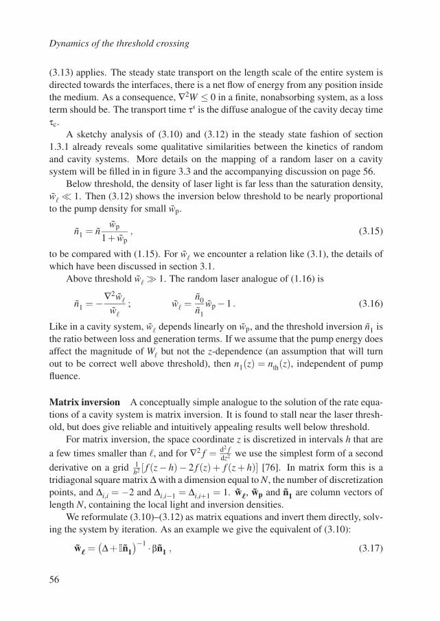
Dynamics of the threshold crossing
(3.13) applies. The steady state transport on the length scale of the entire system isdirected towards the interfaces, there is a net flow of energy from any position insidethe medium. As a consequence, ∇2W ≤ 0 in a finite, nonabsorbing system, as a lossterm should be. The transport time τs is the diffuse analogue of the cavity decay timeτc.
A sketchy analysis of (3.10) and (3.12) in the steady state fashion of section1.3.1 already reveals some qualitative similarities between the kinetics of randomand cavity systems. More details on the mapping of a random laser on a cavitysystem will be filled in in figure 3.3 and the accompanying discussion on page 56.
Below threshold, the density of laser light is far less than the saturation density,w 1. Then (3.12) shows the inversion below threshold to be nearly proportionalto the pump density for small wp.
n1 = nwp
1+ wp, (3.15)
to be compared with (1.15). For w we encounter a relation like (3.1), the details ofwhich have been discussed in section 3.1.
Above threshold w 1. The random laser analogue of (1.16) is
n1 = −∇2w
w
; w =n0
n1wp −1 . (3.16)
Like in a cavity system, w depends linearly on wp, and the threshold inversion n1 isthe ratio between loss and generation terms. If we assume that the pump energy doesaffect the magnitude of W but not the z-dependence (an assumption that will turnout to be correct well above threshold), then n1(z) = nth(z), independent of pumpfluence.
Matrix inversion A conceptually simple analogue to the solution of the rate equa-tions of a cavity system is matrix inversion. It is found to stall near the laser thresh-old, but does give reliable and intuitively appealing results well below threshold.
For matrix inversion, the space coordinate z is discretized in intervals h that area few times smaller than , and for ∇2 f = d2 f
dz2 we use the simplest form of a second
derivative on a grid 1h2 [ f (z− h)− 2 f (z) + f (z + h)] [76]. In matrix form this is a
tridiagonal square matrix ∆ with a dimension equal to N, the number of discretizationpoints, and ∆i,i = −2 and ∆i,i−1 = ∆i,i+1 = 1. w, wp and n1 are column vectors oflength N, containing the local light and inversion densities.
We reformulate (3.10)–(3.12) as matrix equations and invert them directly, solv-ing the system by iteration. As an example we give the equivalent of (3.10):
w =(∆+ In1
)−1 ·βn1 , (3.17)
56
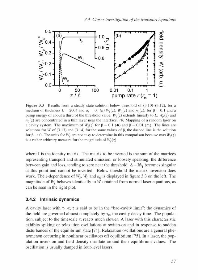
3.4 Closer investigation of the transport equations
0 50 1000.0
0.1
0.2
0.3
0.4
0.5
(a)
Wp
W /
W
s,
Wp /
Wp
s
z /
0.8
0.9
1.0n0
W
n0 / n
0.01 0.1 1
(b)
field
density
W (a
rb. u
.)
pump rate r (rth = 1)
Figure 3.3 Results from a steady state solution below threshold of (3.10)–(3.12), for amedium of thickness L = 200 and σr = 0. (a) W(z), Wp(z) and n0(z), for β = 0.1 and apump energy of about a third of the threshold value. W(z) extends linearly to L. Wp(z) andn0(z) are concentrated in a thin layer near the interface. (b) Mapping of a random laser ona cavity system. The maximum of W(z) for β = 0.1 (•) and β = 0.01 (). The lines aresolutions for W of (3.13) and (3.14) for the same values of β, the dashed line is the solutionfor β → 0. The units for W are not easy to determine in this comparison because maxW(z)is a rather arbitrary measure for the magnitude of W(z).
where I is the identity matrix. The matrix to be inverted is the sum of the matricesrepresenting transport and stimulated emission, or loosely speaking, the differencebetween gain and loss, tending to zero near the threshold. ∆+ In1 becomes singularat this point and cannot be inverted. Below threshold the matrix inversion doeswork. The z-dependence of W, Wp and n0 is displayed in figure 3.3 on the left. Themagnitude of W behaves identically to W obtained from normal laser equations, ascan be seen in the right plot.
3.4.2 Intrinsic dynamics
A cavity laser with τc τ is said to be in the “bad-cavity limit”: the dynamics ofthe field are governed almost completely by τc, the cavity decay time. The popula-tion, subject to the timescale τ, reacts much slower. A laser with this characteristicexhibits spiking or relaxation oscillations at switch-on and in response to suddendisturbances of the equilibrium state [74]. Relaxation oscillations are a general phe-nomenon occurring in nonlinear oscillators off equilibrium [75]. In a laser, the pop-ulation inversion and field density oscillate around their equilibrium values. Theoscillation is usually damped in four-level lasers.
57
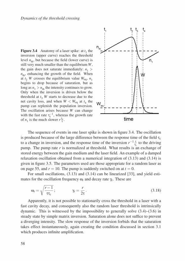
Dynamics of the threshold crossing
Figure 3.4 Anatomy of a laser spike: at t1 theinversion (upper curve) reaches the thresholdlevel nth, but because the field (lower curve) isstill very much smaller than the equilibrium W ,the gain does not saturate immediately: n1 >nth, enhancing the growth of the field. Whenat t2 W crosses the equilibrium value Weq, n1begins to drop because of saturation, but aslong as n1 > nth the intensity continues to grow.Only when the inversion is driven below thethreshold at t3 W starts to decrease due to thenet cavity loss, and when W < Weq at t4 thepump can replenish the population inversion.The oscillation arises because W can changewith the fast rate τ−1
c , whereas the growth rateof n1 is the much slower r τc
τ .
t2t3
t4
t1
nth
n1
Weq
W
time
The sequence of events in one laser spike is shown in figure 3.4. The oscillationis produced because of the large difference between the response time of the field τc
to a change in inversion, and the response time of the inversion r−1 ττc
to the drivingpump. The pump rate r is normalized at threshold. What results is an exchange ofstored energy between the gain medium and the laser field. An example of a dampedrelaxation oscillation obtained from a numerical integration of (3.13) and (3.14) isgiven in figure 3.5. The parameters used are those appropriate for a random laser ason page 55, and r = 10. The pump is suddenly switched on at t = 0.
For small oscillations, (3.13) and (3.14) can be linearized [33], and yield esti-mates for the oscillation frequency ωr and decay rate γr. These are
ωr =√
r−1ττc
; γr =r2τ
. (3.18)
Apparently, it is not possible to stationarily cross the threshold in a laser with afast cavity decay, and consequently also the random laser threshold is intrinsicallydynamic. This is witnessed by the impossibility to generally solve (3.4)–(3.6) insteady state by simple matrix inversion. Saturation alone does not suffice to preventa diverging intensity. The slow response of the inversion forbids that the saturationtakes effect instantaneously, again creating the condition discussed in section 3.1which produces infinite amplification.
58
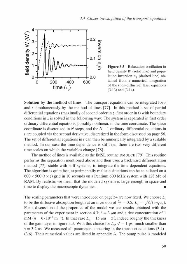
3.4 Closer investigation of the transport equations
0 200 400 600
0
1
2
3
4
field
density W
(W
s
)
time (c)
0.0
0.1
0.2 invers
ion n
1 /n Figure 3.5 Relaxation oscillation infield density W (solid line) and popu-lation inversion n1 (dashed line) ob-tained from a numerical integrationof the (non-diffusive) laser equations(3.13) and (3.14).
Solution by the method of lines The transport equations can be integrated for zand t simultaneously by the method of lines [77]. In this method a set of partialdifferential equations (maximally of second order in z, first order in t) with boundaryconditions in z is solved in the following way: The system is separated in first orderordinary differential equations, possibly nonlinear, in the time coordinate. The spacecoordinate is discretized in N steps, and the N −1 ordinary differential equations int are coupled via the second derivative, discretized in the form discussed on page 56.The set of differential equations in t can then be numerically integrated by a suitablemethod. In our case the time dependence is stiff, i.e. there are two very differenttime scales on which the variables change [78].
The method of lines is available as the IMSL routine DMOLCH [79]. This routineperforms the separation mentioned above and then uses a backward differentiationmethod [77], stable with stiff systems, to integrate the time dependent equations.The algorithm is quite fast, experimentally realistic situations can be calculated on a600×500 (t × z) grid in 10 seconds on a Pentium 600 MHz system with 128 Mb ofRAM. By realistic we mean that the modeled system is large enough in space andtime to display the macroscopic dynamics.
The scaling parameters that were introduced on page 54 are now fixed. We choose Lz
to be the diffusive absorption length at an inversion of n1n = 0.5: Lz =
√/(3n1σa).
For a discussion of the properties of the model we use results obtained with theparameters of the experiment in section 4.3: = 3 µm and a dye concentration of 1mM (n = 6 ·1023 m−3). In that case Lz = 15 µm = 5, indeed roughly the thicknessof the gain layer in figure 3.3. With this choice for Lz, τs = 1 ps, much smaller thanτ = 3.2 ns. We measured all parameters appearing in the transport equations (3.4)–(3.6). Their numerical values are listed in appendix A. The pump pulse is modeled
59
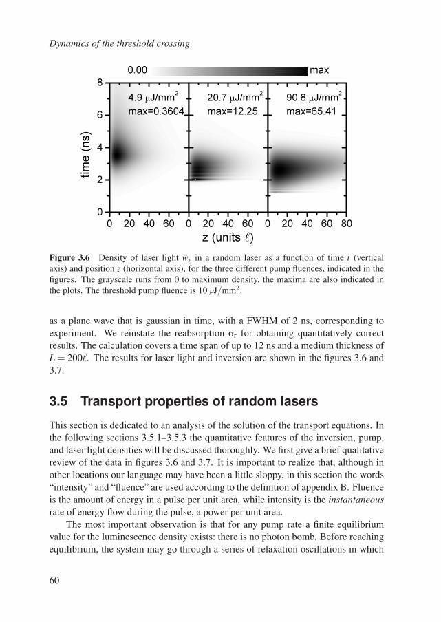
Dynamics of the threshold crossing
0 20 40 60
0
2
4
6
8
tim
e (
ns)
4.9 J/mm2
max=0.3604
0 20 40 60
z (units )
20.7 J/mm2
max=12.25
0 20 40 60 80
90.8 J/mm2
max=65.41
0.00 max
Figure 3.6 Density of laser light w in a random laser as a function of time t (verticalaxis) and position z (horizontal axis), for the three different pump fluences, indicated in thefigures. The grayscale runs from 0 to maximum density, the maxima are also indicated inthe plots. The threshold pump fluence is 10 µJ/mm2.
as a plane wave that is gaussian in time, with a FWHM of 2 ns, corresponding toexperiment. We reinstate the reabsorption σr for obtaining quantitatively correctresults. The calculation covers a time span of up to 12 ns and a medium thickness ofL = 200. The results for laser light and inversion are shown in the figures 3.6 and3.7.
3.5 Transport properties of random lasers
This section is dedicated to an analysis of the solution of the transport equations. Inthe following sections 3.5.1–3.5.3 the quantitative features of the inversion, pump,and laser light densities will be discussed thoroughly. We first give a brief qualitativereview of the data in figures 3.6 and 3.7. It is important to realize that, although inother locations our language may have been a little sloppy, in this section the words“intensity” and “fluence” are used according to the definition of appendix B. Fluenceis the amount of energy in a pulse per unit area, while intensity is the instantaneousrate of energy flow during the pulse, a power per unit area.
The most important observation is that for any pump rate a finite equilibriumvalue for the luminescence density exists: there is no photon bomb. Before reachingequilibrium, the system may go through a series of relaxation oscillations in which
60
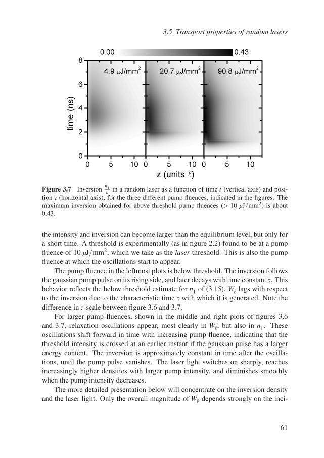
3.5 Transport properties of random lasers
0 5 10
0
2
4
6
8
z (units )
tim
e (
ns)
4.9 J/mm2
0 5 10
20.7 J/mm2
0 5 10
90.8 J/mm2
0.430.00
Figure 3.7 Inversionn1n in a random laser as a function of time t (vertical axis) and posi-
tion z (horizontal axis), for the three different pump fluences, indicated in the figures. Themaximum inversion obtained for above threshold pump fluences (> 10 µJ/mm2) is about0.43.
the intensity and inversion can become larger than the equilibrium level, but only fora short time. A threshold is experimentally (as in figure 2.2) found to be at a pumpfluence of 10 µJ/mm2, which we take as the laser threshold. This is also the pumpfluence at which the oscillations start to appear.
The pump fluence in the leftmost plots is below threshold. The inversion followsthe gaussian pump pulse on its rising side, and later decays with time constant τ. Thisbehavior reflects the below threshold estimate for n1 of (3.15). W lags with respectto the inversion due to the characteristic time τ with which it is generated. Note thedifference in z-scale between figure 3.6 and 3.7.
For larger pump fluences, shown in the middle and right plots of figures 3.6and 3.7, relaxation oscillations appear, most clearly in W, but also in n1. Theseoscillations shift forward in time with increasing pump fluence, indicating that thethreshold intensity is crossed at an earlier instant if the gaussian pulse has a largerenergy content. The inversion is approximately constant in time after the oscilla-tions, until the pump pulse vanishes. The laser light switches on sharply, reachesincreasingly higher densities with larger pump intensity, and diminishes smoothlywhen the pump intensity decreases.
The more detailed presentation below will concentrate on the inversion densityand the laser light. Only the overall magnitude of Wp depends strongly on the inci-
61
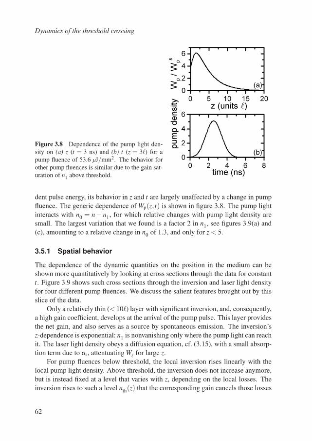
Dynamics of the threshold crossing
Figure 3.8 Dependence of the pump light den-sity on (a) z (t = 3 ns) and (b) t (z = 3) for apump fluence of 53.6 µJ/mm2. The behavior forother pump fluences is similar due to the gain sat-uration of n1 above threshold.
0 5 10 15 200
2
4
6
(a)
pum
p d
ensity
W
p /
Wp
s
z (units )
0 2 4 6 80
2
4
6
(b)
time (ns)
dent pulse energy, its behavior in z and t are largely unaffected by a change in pumpfluence. The generic dependence of Wp(z, t) is shown in figure 3.8. The pump lightinteracts with n0 = n− n1, for which relative changes with pump light density aresmall. The largest variation that we found is a factor 2 in n1, see figures 3.9(a) and(c), amounting to a relative change in n0 of 1.3, and only for z < 5.
3.5.1 Spatial behavior
The dependence of the dynamic quantities on the position in the medium can beshown more quantitatively by looking at cross sections through the data for constantt. Figure 3.9 shows such cross sections through the inversion and laser light densityfor four different pump fluences. We discuss the salient features brought out by thisslice of the data.
Only a relatively thin (< 10) layer with significant inversion, and, consequently,a high gain coefficient, develops at the arrival of the pump pulse. This layer providesthe net gain, and also serves as a source by spontaneous emission. The inversion’sz-dependence is exponential: n1 is nonvanishing only where the pump light can reachit. The laser light density obeys a diffusion equation, cf. (3.15), with a small absorp-tion term due to σr, attentuating W for large z.
For pump fluences below threshold, the local inversion rises linearly with thelocal pump light density. Above threshold, the inversion does not increase anymore,but is instead fixed at a level that varies with z, depending on the local losses. Theinversion rises to such a level nth(z) that the corresponding gain cancels those losses
62
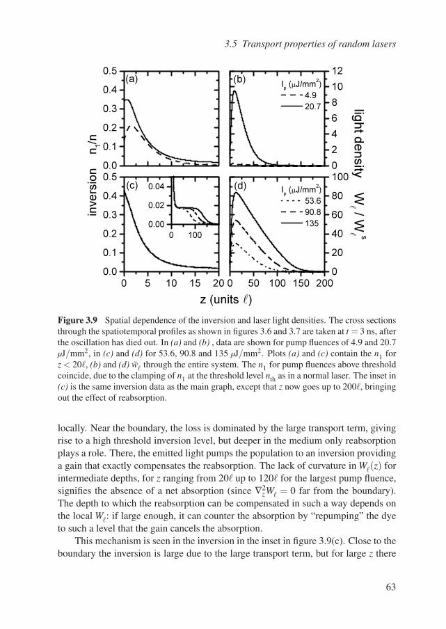
3.5 Transport properties of random lasers
0.0
0.1
0.2
0.3
0.4
0.5(a)
invers
ion
n1/n
0
2
4
6
8
10
12(b)
Ip (J/mm
2)
4.9
20.7
ligh
t de
nsity
W / W
s
0 5 10 15 200.0
0.1
0.2
0.3
0.4
0.5(c)
z (units )
0 50 100 150 2000
20
40
60
80
100(d) I
p (J/mm
2)
53.6
90.8
135
0 100
0.00
0.02
0.04
Figure 3.9 Spatial dependence of the inversion and laser light densities. The cross sectionsthrough the spatiotemporal profiles as shown in figures 3.6 and 3.7 are taken at t = 3 ns, afterthe oscillation has died out. In (a) and (b) , data are shown for pump fluences of 4.9 and 20.7µJ/mm2, in (c) and (d) for 53.6, 90.8 and 135 µJ/mm2. Plots (a) and (c) contain the n1 forz < 20, (b) and (d) w through the entire system. The n1 for pump fluences above thresholdcoincide, due to the clamping of n1 at the threshold level nth as in a normal laser. The inset in(c) is the same inversion data as the main graph, except that z now goes up to 200, bringingout the effect of reabsorption.
locally. Near the boundary, the loss is dominated by the large transport term, givingrise to a high threshold inversion level, but deeper in the medium only reabsorptionplays a role. There, the emitted light pumps the population to an inversion providinga gain that exactly compensates the reabsorption. The lack of curvature in W(z) forintermediate depths, for z ranging from 20 up to 120 for the largest pump fluence,signifies the absence of a net absorption (since ∇2
zW = 0 far from the boundary).The depth to which the reabsorption can be compensated in such a way depends onthe local W: if large enough, it can counter the absorption by “repumping” the dyeto such a level that the gain cancels the absorption.
This mechanism is seen in the inversion in the inset in figure 3.9(c). Close to theboundary the inversion is large due to the large transport term, but for large z there
63
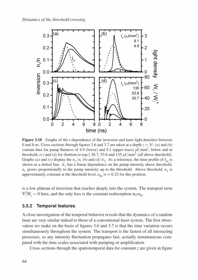
Dynamics of the threshold crossing
0.0
0.1
0.2
0.3
Iin
invers
ion
n1/n
0
1
2
3(b)
Ip (J/mm
2)
9.1
4.9lig
ht d
ensity
W / W
s
0 2 4 6 80.0
0.1
0.2
0.3(c)
time (ns)
0 2 4 6 80
20
40
60
80(d)
(a)
Ip (J/mm
2)
135
53.6
20.7
Figure 3.10 Graphs of the t-dependence of the inversion and laser light densities between0 and 8 ns. Cross sections through figures 3.6 and 3.7 are taken at a depth z = 3. (a) and (b)contain data for pump fluences of 4.9 (lower) and 9.1 (upper trace) µJ/mm2, below and atthreshold, (c) and (d) for (bottom to top:) 20.7, 53.6 and 135 µJ/mm2 (all above threshold).Graphs (a) and (c) display the n1/n, (b) and (d) w. As a reference, the time profile of Iin isshown as a dotted line. w has a linear dependence on the pump intensity above threshold.n1 grows proportionally to the pump intensity up to the threshold. Above threshold, n1 isapproximately constant at the threshold level, nth/n ≈ 0.23 for this position.
is a low plateau of inversion that reaches deeply into the system. The transport term∇2
zW = 0 here, and the only loss is the constant reabsorption σrcn0.
3.5.2 Temporal features
A close investigation of the temporal behavior reveals that the dynamics of a randomlaser are very similar indeed to those of a conventional laser system. The first obser-vation we make on the basis of figures 3.6 and 3.7 is that the time variation occurssimultaneously throughout the system. The transport is the fastest of all interactingprocesses, so any intensity fluctuation propagates fast, actually instantaneous com-pared with the time scales associated with pumping or amplification.
Cross sections through the spatiotemporal data for constant z are given in figure
64
3.5 Transport properties of random lasers
3.10. The population inversion increases proportionally to the pump intensity un-til the threshold inversion nth is reached, nth/n ≈ 0.23 for z = 3 as in figure 3.10.nth(z) can be found in figure 3.9(c). Then the system goes through the relaxationoscillation, of which the details will be discussed later. As can be seen in the data infigure 3.10(c), the above-threshold inversion level is approximately constant. Oncethe pump threshold intensity is crossed in the downward direction, i.e. the energysupply rate is insufficient to keep up a gain that compensates the losses, the popula-tion starts to decay spontaneously, seen here as an exponential tail for t > 5.5 ns infigures 3.10(a) and (c).
The laser light density for low pump fluence is very small, basically only spon-taneous emission, and has a delay τ with respect to the pump pulse, cf. the lowertrace in figure 3.10(b). For 9.1 µJ/mm2 the system just touches on threshold, afterone spike the pump intensity has already dropped below the threshold level. Abovethreshold, for higher pump fluence, the laser light density depends linearly on thepump intensity, as shown in figure 3.10(d).
Slicing figures 3.6 and 3.7 along the time direction allows a quantitative com-parison of the relaxation oscillation with the predictions from cavity laser equationswith small fluctuations. The linearization is unfortunately not as easy in the ran-dom laser transport equations (3.4)–(3.6), because of the space derivative. But it ispossible to compare the results obtained from the numerical solution with (3.18).
As suggested by the analogy between transport and loss, noted on page 56, weuse the characteristic transport time τs = 1 ps for the cavity loss time τc in (3.18).For pump rates r between 1 and 10 (with the threshold rth = 1), the range discussedabove, we estimate an oscillation period 2π/ωr ∼ 100 ps, and a decay time γ−1
r ∼ 1ns, to be compared with results from the dynamic calculation as displayed in figure3.11. The γ−1
r from the calculation is actually about a factor 2 smaller than estimated,caused by the rising pump rate at threshold, which enhances the damping during theoscillation. In general the agreement between the estimate from elementary lasertheory and numerical result for random lasers is satisfactory.
3.5.3 Laser threshold and the explosion
In the previous section, we have identified two regimes for random lasers, as a func-tion of pump intensity: a low pump rate regime where the inversion and the emittedlight density behave as in a normal laser below, and a high pump rate regime corre-sponding to a laser above threshold. The transition between the two is accompaniedby an oscillatory instability. We can therefore say that a random laser does have well-defined threshold, and that it comes about in a way that is similar to the thresholdin a normal laser: a balance between gain and loss. What is particular to a randomlaser is the transport nature of the loss, necessitating a local description of the laser
65
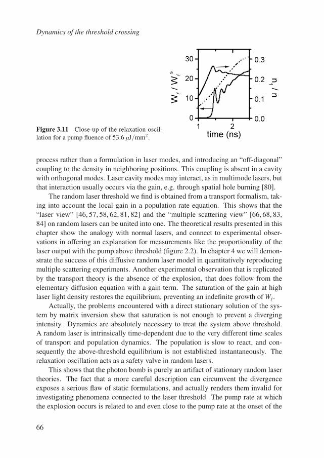
Dynamics of the threshold crossing
Figure 3.11 Close-up of the relaxation oscil-lation for a pump fluence of 53.6 µJ/mm2.
1 2
0
10
20
30
W /
W
s
time (ns)
0.0
0.1
0.2
0.3
n1 / n
process rather than a formulation in laser modes, and introducing an “off-diagonal”coupling to the density in neighboring positions. This coupling is absent in a cavitywith orthogonal modes. Laser cavity modes may interact, as in multimode lasers, butthat interaction usually occurs via the gain, e.g. through spatial hole burning [80].
The random laser threshold we find is obtained from a transport formalism, tak-ing into account the local gain in a population rate equation. This shows that the“laser view” [46, 57, 58, 62, 81, 82] and the “multiple scattering view” [66, 68, 83,84] on random lasers can be united into one. The theoretical results presented in thischapter show the analogy with normal lasers, and connect to experimental obser-vations in offering an explanation for measurements like the proportionality of thelaser output with the pump above threshold (figure 2.2). In chapter 4 we will demon-strate the success of this diffusive random laser model in quantitatively reproducingmultiple scattering experiments. Another experimental observation that is replicatedby the transport theory is the absence of the explosion, that does follow from theelementary diffusion equation with a gain term. The saturation of the gain at highlaser light density restores the equilibrium, preventing an indefinite growth of W.
Actually, the problems encountered with a direct stationary solution of the sys-tem by matrix inversion show that saturation is not enough to prevent a divergingintensity. Dynamics are absolutely necessary to treat the system above threshold.A random laser is intrinsically time-dependent due to the very different time scalesof transport and population dynamics. The population is slow to react, and con-sequently the above-threshold equilibrium is not established instantaneously. Therelaxation oscillation acts as a safety valve in random lasers.
This shows that the photon bomb is purely an artifact of stationary random lasertheories. The fact that a more careful description can circumvent the divergenceexposes a serious flaw of static formulations, and actually renders them invalid forinvestigating phenomena connected to the laser threshold. The pump rate at whichthe explosion occurs is related to and even close to the pump rate at the onset of the
66
3.5 Transport properties of random lasers
oscillation that signals the threshold crossing, but is not the same per se.
3.5.4 Comparison with earlier work
In this chapter we have demonstrated that in a realistic system the explosion doesnot exist, and consequently is not the same as a laser threshold, which does exist.At the laser threshold the population inversion is fixed at a level where the (local)gain exactly compensates the (local) loss, like in an ordinary laser the modal gainequals the modal loss. We have introduced β for a random laser, the fraction ofspontaneous emission contributing to the laser process. The validity of the modelwill be established by a quantitative comparison with measurements in chapter 4.
Earlier explorations of the realm of dynamic random laser theory were made, theimportant references are the works of Letokhov [48], Berger, Kempe, and Genack[60], and Wiersma and Lagendijk [71]. There are three aspects to the work describedin this chapter by which it augments the theory of these references:
the definition of the β-factor, using experimentally accessible quantities;
the elaborate interpretation of transport phenomena in terms of laser termi-nology, most importantly the identification of the transport as the quantitativeequivalent of cavity loss;
the possibility to compare directly with experiments, also by inclusion of thereabsorption term.
We give a brief review of other theoretical work to compare it with our own.Our theory, like the one in ref. 71, can not treat emission line narrowing or other
spectral features in detail. We take the effect of spectral narrowing into accountin β, but the occurrence of e.g. a second laser peak [81, 85] can not be handled.The works by Letokhov [48] and by Berger and coworkers [60] make it possible tostudy spectral dependence. Berger et al. use a Monte Carlo simulation to study thedynamics of the system, and this can be done for a distribution of frequencies. Butthe method suffers from a general limitation of Monte Carlo simulations: it is verytime consuming to study long times and large systems. This makes it difficult touse the results for a study of the common experiments with nanosecond excitationpulse lengths. They do explain the short pulse output observed by Siddique et al.[58], that is due to the occurrence of one laser spike during the picosecond pumppulse. Letokhov develops a formalism that is very general, but only numericallytractable for weak scattering and small gain. For a solution he assumes homogeneouspumping, negligible saturation and a spherical geometry which makes comparisonwith real systems difficult. Unlike Berger and coworkers, Letokhov does not find alimit to the linewidth above threshold.
67
Dynamics of the threshold crossing
John and Pang [86] calculate the line narrowing with a theory that models thepopulation dynamically, but uses a static description for the transport. Their resultsfor the laser threshold, which is not very accurately defined, depend strongly on dyeparameters which we find to be of no importance, such as the rate at which the tripletstate is populated. In their calculation they do use a formalism which resembles ourdiscussion of the β-factor.
Wiersma and Lagendijk [71] integrate a set of equations like (3.4)–(3.6) in amanner that is similar to our calculation, for parameters that are appropriate to asystem consisting of Ti:sapphire powder. The pump energies needed to reach thethreshold are however not easy to realize, unfortunately precluding an experimentaltest of the model. They include a probe beam, separate from the emitted laser light.Because we distinguish between spontaneous emission and laser light by β, a probebeam could be added in our equations by a simple source term like Iin.
A completely different, but dynamic nonetheless, approach is taken by Jiang andSoukoulis [87]. They solve the Maxwell equations for the field coupled to four-levelrate equations for the gain in a one-dimensional disordered system by the finite-difference time domain (FDTD) method. This technique is basically a direct nu-merical integration in time of the Maxwell equations, in a medium with a variationin dielectric constant on a space grid. One calculates the microscopic field, so thespace and time discretizations have to be very finely grained, much smaller than thewavelength and the optical cycle. Because the time step is so small, one has to takeall four levels of the gain medium into consideration. The time of evolution one cancalculate is consequently much smaller than with a diffusion theory, on the otherhand the amount of detail is much larger. This detailed information is used to obtainthe frequency spectrum by Fourier transforming the field in time.
This approach is used to explain the observation of narrow frequency structure inthe emission of random lasers, supposedly due to Anderson localized modes. Jiangand Soukoulis find strong localized modes that are very sharp due to the amplifica-tion in the system. They use parameters appropriate to a concentrated dye solutionwith ZnO scatterers, modeling a system consisting of randomly spaced layers. Thefrequency spikes are the subject of chapter 5, but we discuss the calculations of ref.87 here, because they can be used to illustrate the interpretation of our own results.In disordered materials the dimensionality of the system is crucial [88]: in 1D and 2Drandom media waves are always localized. This is caused by the fact that, whateverthe strength of the disorder, a one- or two-dimensional random walk will eventu-ally return to its starting point with probability one. Transport is inhibited in sucha system. The only way for the wave to escape is to make the sample shorter thanthe localization length, i.e. the extent of the localized state. The localization lengthdepends on the strength of the disorder.
68
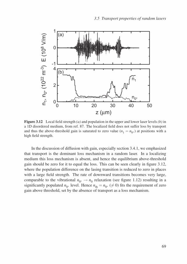
3.5 Transport properties of random lasers
n1,
n0
* (1
02
2 m
-3)
E (
10
8 V
/m)
0
2
-1
0
1
4
0 10 20 30 40 50
z (µm)
n1
n0*
(a)
(b)
Figure 3.12 Local field strength (a) and population in the upper and lower laser levels (b) ina 1D disordered medium, from ref. 87. The localized field does not suffer loss by transportand thus the above-threshold gain is saturated to zero value (n1 = n0∗) at positions with ahigh field strength.
In the discussion of diffusion with gain, especially section 3.4.1, we emphasizedthat transport is the dominant loss mechanism in a random laser. In a localizingmedium this loss mechanism is absent, and hence the equilibrium above-thresholdgain should be zero for it to equal the loss. This can be seen clearly in figure 3.12,where the population difference on the lasing transition is reduced to zero in placeswith a large field strength. The rate of downward transitions becomes very large,comparable to the vibrational n0∗ → n0 relaxation (see figure 1.12) resulting in asignificantly populated n0∗ level. Hence nth = n0∗ ( = 0) fits the requirement of zerogain above threshold, set by the absence of transport as a loss mechanism.
69

4.Interference in random lasers
This chapter describes experiments in which the amplification of a probe beamis used for studying light propagation in a random laser. We have performedmeasurements on speckle in the scattered and amplified light, which is discussedfirst. The second part of this chapter is about enhanced backscattering. We presentthe first high quality enhanced backscattering measurements in a random laser thatcan be driven above the laser threshold, providing experimental insight in the effectof the threshold on light transport. The results of these measurements are shown tobe in quantitative agreement with the theory developed in chapter 3.
In the experiments described in chapter 2 we observed the fluorescence emitted bya random laser to infer the influence of the characteristic length scales in diffusetransport on the laser threshold. The fluorescence is generated by the system itselfand consequently details like directionality, coherence or spectral content can notbe used as experimental parameters. When studying the light transport itself, it isdesirable to have the ability to control the properties of the light source. This is mostconveniently done by using an external beam incident on the sample. We then havea source of diffusing light with known properties, and by measuring the scatteredlight we can investigate the transport of light in the medium. Much is known abouttransport in passive disordered systems from light scattering experiments, and wecan assess the effect of amplification in multiple scattering by comparing data fromrandom lasers with results for ordinary random systems.
4.1 Experimental considerations
Probe beams are used in the experiments presented in this chapter, with a wavelengththat can be amplified by the dye in the medium. The intensity of the incident probe
71
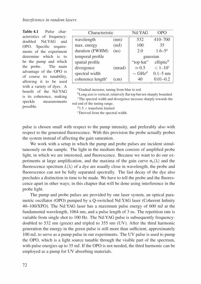
Interference in random lasers
Table 4.1 Pulse char-acteristics of frequency-doubled Nd:YAG andOPO. Specific require-ments of the experimentdetermine which is tobe the pump and whichthe probe. The mainadvantage of the OPO isof course its tunability,allowing it to be usedwith a variety of dyes. Abenefit of the Nd:YAGis its coherence, makingspeckle measurementspossible.
Characteristic Nd:YAG OPO
wavelength (nm) 532 410–700max. energy (mJ) 100 35duration (FWHM) (ns) 2.0 1.6–5a
temporal profile gaussianspatial profile “top hat” ellipticb
divergence (mrad) ≈ 0.5 < 1–10c
spectral width ∼ GHzd 0.1–5 nmcoherence lengthe (cm) 40 0.01–0.2
aGradual increase, tuning from blue to red.bLong axis is vertical; relatively flat top but not sharply bounded.cThe spectral width and divergence increase sharply towards the
red end of the tuning range.d1.5 × transform limitedeDerived from the spectral width.
pulse is chosen small with respect to the pump intensity, and preferably also withrespect to the generated fluorescence. With this provision the probe actually probesthe system instead of affecting the gain saturation.
We work with a setup in which the pump and probe pulses are incident simul-taneously on the sample. The light in the medium then consists of amplified probelight, in which we are interested, and fluorescence. Because we want to do our ex-periments at large amplification, and the maxima of the gain curve σe(λ) and thefluorescence spectrum L(λ) of a dye are usually close in wavelength, the probe andfluorescence can not be fully separated spectrally. The fast decay of the dye alsoprecludes a distinction in time to be made. We have to tell the probe and the fluores-cence apart in other ways; in this chapter that will be done using interference in theprobe light.
The pump and probe pulses are provided by one laser system, an optical para-metric oscillator (OPO) pumped by a Q-switched Nd:YAG laser (Coherent Infinity40–100/XPO). The Nd:YAG laser has a maximum pulse energy of 600 mJ at thefundamental wavelength, 1064 nm, and a pulse length of 3 ns. The repetition rate isvariable from single shot to 100 Hz. The Nd:YAG pulse is subsequently frequency-doubled to 532 nm (green) and tripled to 355 nm (UV). After the third harmonicgeneration the energy in the green pulse is still more than sufficient, approximately100 mJ, to serve as a pump pulse in our experiments. The UV pulse is used to pumpthe OPO, which is a light source tunable through the visible part of the spectrum,with pulse energies up to 35 mJ. If the OPO is not needed, the third harmonic can beemployed as a pump for UV absorbing materials.
72
4.2 Speckle in random lasers
Depending on the requirements on the pump and probe beams, we can chooseto use either the second harmonic of the Nd:YAG laser as a pump and the OPO asa probe or vice versa. There are a number of characteristics in which the pulsesdiffer; a summary is given in table 4.1. It shows that the properties of the OPO pulsedepend strongly on the set wavelength, and in general degrade towards the red sideof the tuning range. The energy in the OPO pulse is large, but the moderate beamquality necessitates spatial filtering (except perhaps for λ < 480 nm), which reducesthe usable energy by a factor 50.
For OPO power regulation we use a set of polarizing Glan laser prisms. Thefirst is rotated to vary the amount of power, while the second selects the transmittedpolarization, compatible with the mirrors used. A drawback of this setup is the steepintensity change at small transmission (I ∝ sin4 α, where α is the rotation angle). Theadvantage is its wavelength independence. For the Nd:YAG we use a rotating λ/2retardation plate mounted between two crossed Glan prism polarizers. In this casethe sensitivity for small transmissions is better (I ∝ sin2 α).
Getting pump and probe pulses from the same laser system has the advantagethat the timing of the experiment becomes particularly simple. The jitter betweenthe pulses is minimal and the difference in arrival times can be easily compensatedby optical delay. We put a delay line in the pump beam path, because the probebeam alignment is much more precarious than the pump, and might be disturbed bymoving a slightly imperfectly aligned delay line. The Nd:YAG pulse is the leadingone. Several ns of variable delay is convenient for optimization; the delay line has alength of maximally 2×1.5 m.
4.2 Speckle in random lasers
Speckle is the strongly fluctuating, grainy intensity pattern resulting from the inter-ference of a randomly scattered coherent wave. It can be observed in space, time andfrequency. Some statistical characteristics of the speckle pattern contain informationabout the transport process [89]. We discuss only speckle in space, i.e. a fluctuatingintensity with angle.
If a coherent plane wave falls on a rough surface, a speckle pattern can be seenon a screen positioned at some distance from the scattering object. The scatteredfields at a certain position on the screen comes from all points of the rough surface,and its random phases distributed uniformly between 0 and 2π. The speckle is theaddition of the electric field vectors of all the N contributing partial waves. Thesummation constitutes a random walk in the complex plane, with a resulting fieldE = 1/
√N ∑k ak exp(iφk) [90].
The sum results in a gaussian distribution for E, with most probable value E = 0
73
Interference in random lasers
and variance 〈|E|2〉= limN→∞(2N)−1 ∑k〈|ak|2〉. The observed intensity I = |E|2 thenfollows a Rayleigh distribution:
P(I) =1〈I〉e−
I〈I〉 . (4.1)
The typical speckle spot size depends on the characteristic distance along thescreen on which the fields that contribute to the speckle dephase. The largest pathlength difference at a spot on the screen is caused by the partial waves arriving fromopposite ends of the illuminated region of the scattering surface. Consequently, thetypical angular size of a speckle spot is λ/d [90], if d is the diameter of the illu-minated region. This demonstrates that a measurement of the speckle spot size, forinstance by the autocorrelation of the speckle pattern, does not usually give infor-mation about light inside a scattering medium. The spot size in reflection dependsmainly on the incident beam diameter. In transmission the most influential parame-ter is the sample thickness, which determines the degree to which an incident pointsource spreads in transport to the rear interface.
The field of speckle experiments in random lasers is largely uncharted territory.The only data available of the effect of gain on a speckle pattern produced by a probebeam are those of ref. 91. Refs. 92 and 93 study the related subject of coherenceproperties of the generated light. In this section we present experimental resultsconcerning the intensity statistics and speckle spot size. In contrast with passivesystems, these measurements do depend on parameters of light transport. There isno theory to compare the measurements with. We will give qualitative explanationsof the results.
Theoretical studies of speckle in random lasers [66, 94–96] invariably investi-gate speckle correlations. While interesting, these correlations are exprimentallynot easily accessible, for reasons that will be discussed in section 4.2.4. A furtherlimitation of the theoretical efforts in this field is that they all rely on a stationaryformalism, with fixed gain, so they encounter the explosion when approaching thelaser threshold.
4.2.1 Sample and setup
Spatial speckle can only be observed if the coherence length of the light is muchlarger than the maximum path length difference between partial waves contributingto speckle. In the region where the rhodamine dyes fluoresce the OPO beam has alinewidth that is too large to produce speckle with a good contrast: its coherence isinsufficient. The frequency-doubled Nd:YAG can be amplified by a dye with a largegain at 532 nm, such as Coumarin 6 (see appendix A). In dye lasers it is usually dis-solved in ethylene glycol, but unfortunately our TiO2 [44] colloid is not suspended
74
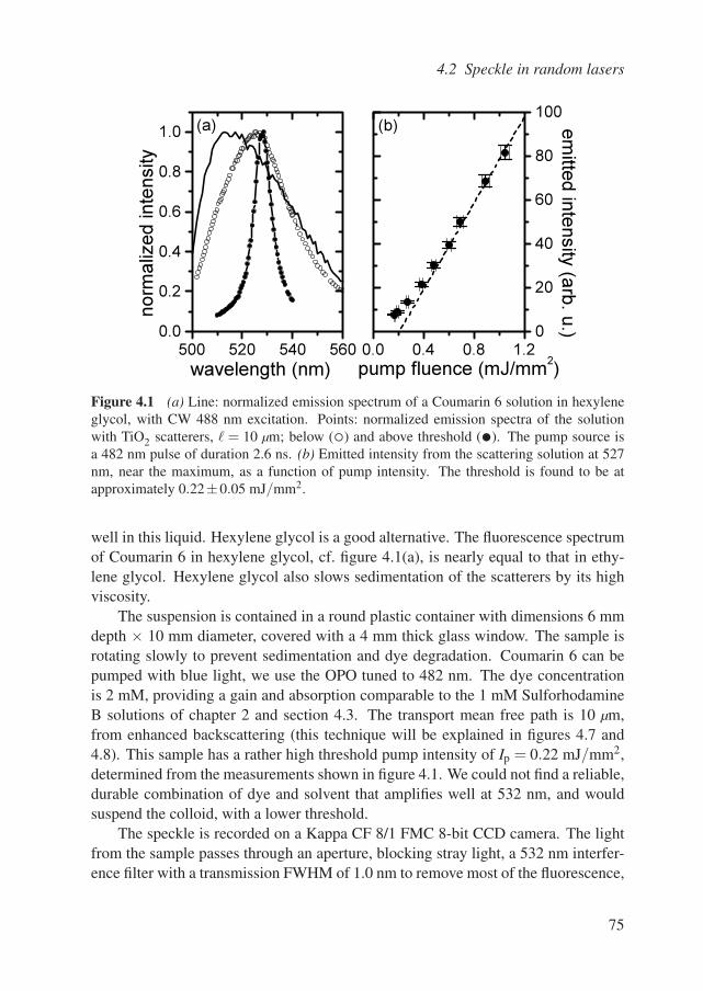
4.2 Speckle in random lasers
500 520 540 5600.0
0.2
0.4
0.6
0.8
1.0 (a)
norm
aliz
ed inte
nsity
wavelength (nm)0.0 0.4 0.8 1.2
0
20
40
60
80
100(b)
em
itted in
tensity
(arb
. u.)
pump fluence (mJ/mm2
)
Figure 4.1 (a) Line: normalized emission spectrum of a Coumarin 6 solution in hexyleneglycol, with CW 488 nm excitation. Points: normalized emission spectra of the solutionwith TiO2 scatterers, = 10 µm; below () and above threshold (•). The pump source isa 482 nm pulse of duration 2.6 ns. (b) Emitted intensity from the scattering solution at 527nm, near the maximum, as a function of pump intensity. The threshold is found to be atapproximately 0.22±0.05 mJ/mm2.
well in this liquid. Hexylene glycol is a good alternative. The fluorescence spectrumof Coumarin 6 in hexylene glycol, cf. figure 4.1(a), is nearly equal to that in ethy-lene glycol. Hexylene glycol also slows sedimentation of the scatterers by its highviscosity.
The suspension is contained in a round plastic container with dimensions 6 mmdepth × 10 mm diameter, covered with a 4 mm thick glass window. The sample isrotating slowly to prevent sedimentation and dye degradation. Coumarin 6 can bepumped with blue light, we use the OPO tuned to 482 nm. The dye concentrationis 2 mM, providing a gain and absorption comparable to the 1 mM SulforhodamineB solutions of chapter 2 and section 4.3. The transport mean free path is 10 µm,from enhanced backscattering (this technique will be explained in figures 4.7 and4.8). This sample has a rather high threshold pump intensity of Ip = 0.22 mJ/mm2,determined from the measurements shown in figure 4.1. We could not find a reliable,durable combination of dye and solvent that amplifies well at 532 nm, and wouldsuspend the colloid, with a lower threshold.
The speckle is recorded on a Kappa CF 8/1 FMC 8-bit CCD camera. The lightfrom the sample passes through an aperture, blocking stray light, a 532 nm interfer-ence filter with a transmission FWHM of 1.0 nm to remove most of the fluorescence,
75
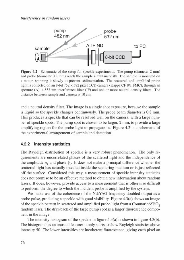
Interference in random lasers
pump
482 nmprobe
532 nm
sampleA IF ND
8-bit CCD
to PC
Figure 4.2 Schematic of the setup for speckle experiments. The pump (diameter 2 mm)and probe (diameter 0.8 mm) reach the sample simultaneously. The sample is mounted ona motor, spinning it slowly to prevent sedimentation. The scattered and amplified probelight is collected on an 8-bit 752×582 pixel CCD camera (Kappa CF 8/1 FMC), through anaperture (A), a 532 nm interference filter (IF) and one or more neutral density filters. Thedistance between sample and camera is 10 cm.
and a neutral density filter. The image is a single shot exposure, because the sampleis liquid so the speckle changes continuously. The probe beam diameter is 0.8 mm.This produces a speckle that can be resolved well on the camera, with a large num-ber of speckle spots. The pump spot is chosen to be larger, 2 mm, to provide a largeamplifying region for the probe light to propagate in. Figure 4.2 is a schematic ofthe experimental arrangement of sample and detection.
4.2.2 Intensity statistics
The Rayleigh distribution of speckle is a very robust phenomenon. The only re-quirements are uncorrelated phases of the scattered light and the independence ofthe amplitude ak and phase φk. It does not make a principal difference whether thescattered light has actually traveled inside the scattering medium or is just reflectedoff the surface. Considered this way, a measurement of speckle intensity statisticsdoes not promise to be an effective method to obtain new information about randomlasers. It does, however, provide access to a measurement that is otherwise difficultto perform: the degree to which the incident probe is amplified by the system.
We make use of the coherence of the Nd:YAG frequency doubled output as aprobe pulse, producing a speckle with good visibility. Figure 4.3(a) shows an imageof the speckle pattern in scattered and amplified probe light from a Coumarin6/TiO2random laser. The drawback of the large pump spot is a larger fluorescence compo-nent in the image.
The intensity histogram of the speckle in figure 4.3(a) is shown in figure 4.3(b).The histogram has an unusual feature: it only starts to show Rayleigh statistics aboveintensity 50. The lower intensities are incoherent fluorescence, giving each pixel an
76
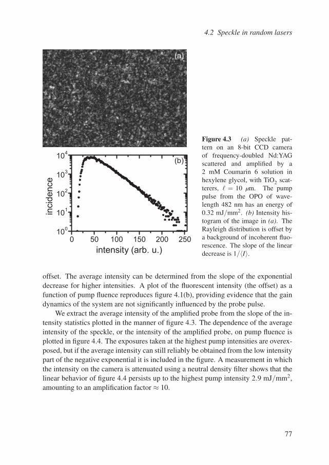
4.2 Speckle in random lasers
(a)
100
101
102
103
104
(b)
incid
ence
intensity (arb. u.)
0 50 100 150 200 250
Figure 4.3 (a) Speckle pat-tern on an 8-bit CCD cameraof frequency-doubled Nd:YAGscattered and amplified by a2 mM Coumarin 6 solution inhexylene glycol, with TiO2 scat-terers, = 10 µm. The pumppulse from the OPO of wave-length 482 nm has an energy of0.32 mJ/mm2. (b) Intensity his-togram of the image in (a). TheRayleigh distribution is offset bya background of incoherent fluo-rescence. The slope of the lineardecrease is 1/〈I〉.
offset. The average intensity can be determined from the slope of the exponentialdecrease for higher intensities. A plot of the fluorescent intensity (the offset) as afunction of pump fluence reproduces figure 4.1(b), providing evidence that the gaindynamics of the system are not significantly influenced by the probe pulse.
We extract the average intensity of the amplified probe from the slope of the in-tensity statistics plotted in the manner of figure 4.3. The dependence of the averageintensity of the speckle, or the intensity of the amplified probe, on pump fluence isplotted in figure 4.4. The exposures taken at the highest pump intensities are overex-posed, but if the average intensity can still reliably be obtained from the low intensitypart of the negative exponential it is included in the figure. A measurement in whichthe intensity on the camera is attenuated using a neutral density filter shows that thelinear behavior of figure 4.4 persists up to the highest pump intensity 2.9 mJ/mm2,amounting to an amplification factor ≈ 10.
77
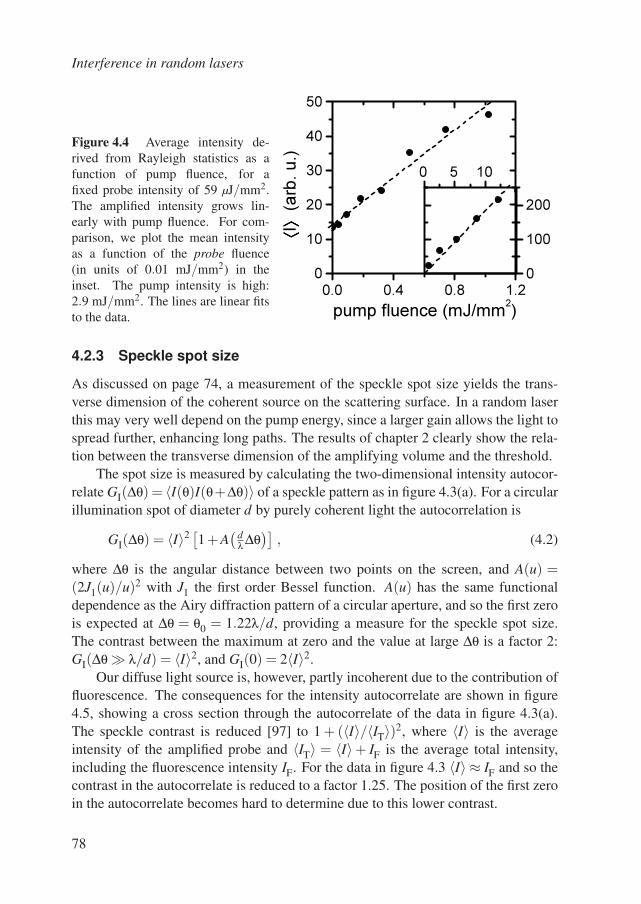
Interference in random lasers
Figure 4.4 Average intensity de-rived from Rayleigh statistics as afunction of pump fluence, for afixed probe intensity of 59 µJ/mm2.The amplified intensity grows lin-early with pump fluence. For com-parison, we plot the mean intensityas a function of the probe fluence(in units of 0.01 mJ/mm2) in theinset. The pump intensity is high:2.9 mJ/mm2. The lines are linear fitsto the data.
0.0 0.4 0.8 1.2
0
10
20
30
40
50
I
(arb
. u.)
pump fluence (mJ/mm2
)
0 5 10
0
100
200
4.2.3 Speckle spot size
As discussed on page 74, a measurement of the speckle spot size yields the trans-verse dimension of the coherent source on the scattering surface. In a random laserthis may very well depend on the pump energy, since a larger gain allows the light tospread further, enhancing long paths. The results of chapter 2 clearly show the rela-tion between the transverse dimension of the amplifying volume and the threshold.
The spot size is measured by calculating the two-dimensional intensity autocor-relate GI(∆θ) = 〈I(θ)I(θ+∆θ)〉 of a speckle pattern as in figure 4.3(a). For a circularillumination spot of diameter d by purely coherent light the autocorrelation is
GI(∆θ) = 〈I〉2 [1+A
(dλ ∆θ
)], (4.2)
where ∆θ is the angular distance between two points on the screen, and A(u) =(2J1(u)/u)2 with J1 the first order Bessel function. A(u) has the same functionaldependence as the Airy diffraction pattern of a circular aperture, and so the first zerois expected at ∆θ = θ0 = 1.22λ/d, providing a measure for the speckle spot size.The contrast between the maximum at zero and the value at large ∆θ is a factor 2:GI(∆θ λ/d) = 〈I〉2, and GI(0) = 2〈I〉2.
Our diffuse light source is, however, partly incoherent due to the contribution offluorescence. The consequences for the intensity autocorrelate are shown in figure4.5, showing a cross section through the autocorrelate of the data in figure 4.3(a).The speckle contrast is reduced [97] to 1 + (〈I〉/〈IT〉)2, where 〈I〉 is the averageintensity of the amplified probe and 〈IT〉 = 〈I〉+ IF is the average total intensity,including the fluorescence intensity IF. For the data in figure 4.3 〈I〉 ≈ IF and so thecontrast in the autocorrelate is reduced to a factor 1.25. The position of the first zeroin the autocorrelate becomes hard to determine due to this lower contrast.
78
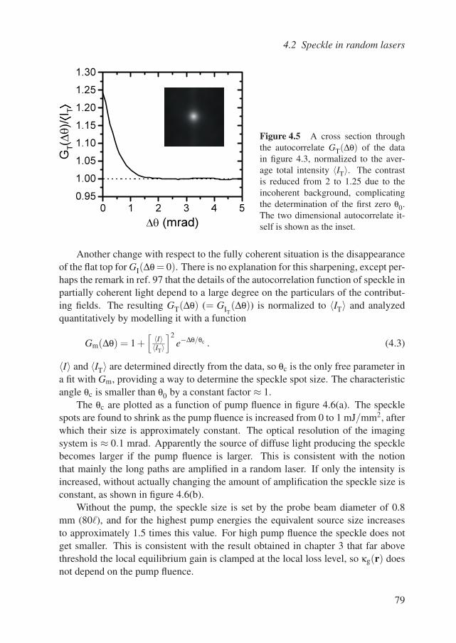
4.2 Speckle in random lasers
0 1 2 3 4 5
0.95
1.00
1.05
1.10
1.15
1.20
1.25
1.30
G
T()/ I
T
(mrad)
Figure 4.5 A cross section throughthe autocorrelate GT(∆θ) of the datain figure 4.3, normalized to the aver-age total intensity 〈IT〉. The contrastis reduced from 2 to 1.25 due to theincoherent background, complicatingthe determination of the first zero θ0.The two dimensional autocorrelate it-self is shown as the inset.
Another change with respect to the fully coherent situation is the disappearanceof the flat top for GI(∆θ = 0). There is no explanation for this sharpening, except per-haps the remark in ref. 97 that the details of the autocorrelation function of speckle inpartially coherent light depend to a large degree on the particulars of the contribut-ing fields. The resulting GT(∆θ) (= GIT
(∆θ)) is normalized to 〈IT〉 and analyzedquantitatively by modelling it with a function
Gm(∆θ) = 1+[ 〈I〉〈IT〉
]2e−∆θ/θc . (4.3)
〈I〉 and 〈IT〉 are determined directly from the data, so θc is the only free parameter ina fit with Gm, providing a way to determine the speckle spot size. The characteristicangle θc is smaller than θ0 by a constant factor ≈ 1.
The θc are plotted as a function of pump fluence in figure 4.6(a). The specklespots are found to shrink as the pump fluence is increased from 0 to 1 mJ/mm2, afterwhich their size is approximately constant. The optical resolution of the imagingsystem is ≈ 0.1 mrad. Apparently the source of diffuse light producing the specklebecomes larger if the pump fluence is larger. This is consistent with the notionthat mainly the long paths are amplified in a random laser. If only the intensity isincreased, without actually changing the amount of amplification the speckle size isconstant, as shown in figure 4.6(b).
Without the pump, the speckle size is set by the probe beam diameter of 0.8mm (80), and for the highest pump energies the equivalent source size increasesto approximately 1.5 times this value. For high pump fluence the speckle does notget smaller. This is consistent with the result obtained in chapter 3 that far abovethreshold the local equilibrium gain is clamped at the local loss level, so κg(r) doesnot depend on the pump fluence.
79
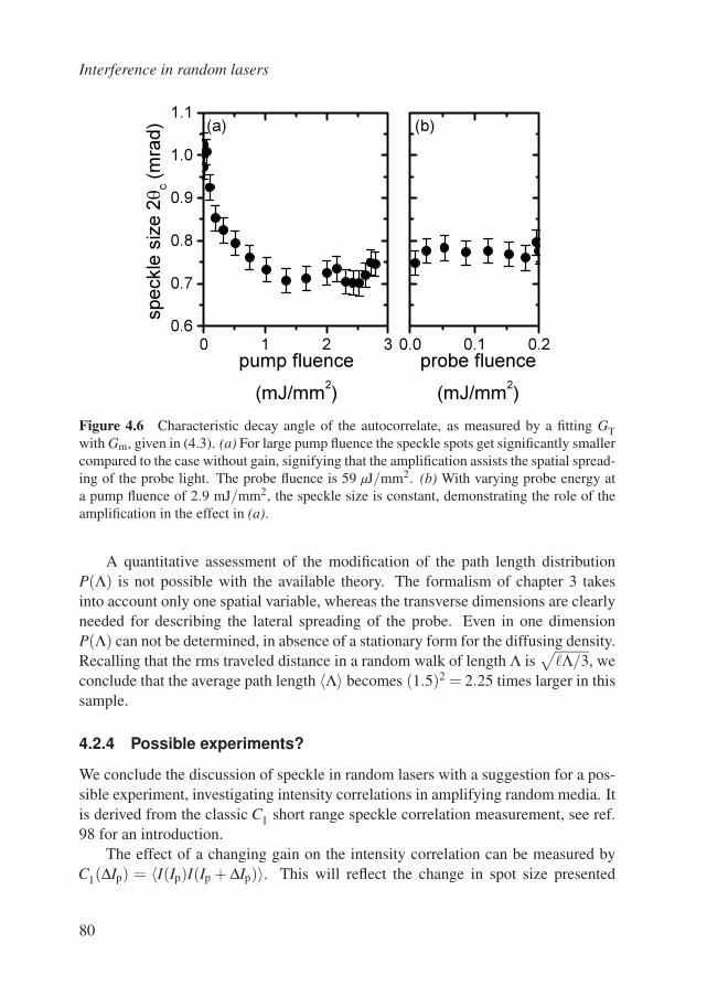
Interference in random lasers
0 1 2 30.6
0.7
0.8
0.9
1.0
1.1(a)
probe fluence
(mJ/mm2
)
pump fluence
(mJ/mm2
)
speckle
siz
e 2c (
mra
d)
0.0 0.1 0.2
(b)
Figure 4.6 Characteristic decay angle of the autocorrelate, as measured by a fitting GTwith Gm, given in (4.3). (a) For large pump fluence the speckle spots get significantly smallercompared to the case without gain, signifying that the amplification assists the spatial spread-ing of the probe light. The probe fluence is 59 µJ/mm2. (b) With varying probe energy ata pump fluence of 2.9 mJ/mm2, the speckle size is constant, demonstrating the role of theamplification in the effect in (a).
A quantitative assessment of the modification of the path length distributionP(Λ) is not possible with the available theory. The formalism of chapter 3 takesinto account only one spatial variable, whereas the transverse dimensions are clearlyneeded for describing the lateral spreading of the probe. Even in one dimensionP(Λ) can not be determined, in absence of a stationary form for the diffusing density.Recalling that the rms traveled distance in a random walk of length Λ is
√Λ/3, we
conclude that the average path length 〈Λ〉 becomes (1.5)2 = 2.25 times larger in thissample.
4.2.4 Possible experiments?
We conclude the discussion of speckle in random lasers with a suggestion for a pos-sible experiment, investigating intensity correlations in amplifying random media. Itis derived from the classic C1 short range speckle correlation measurement, see ref.98 for an introduction.
The effect of a changing gain on the intensity correlation can be measured byC1(∆Ip) = 〈I(Ip)I(Ip + ∆Ip)〉. This will reflect the change in spot size presented
80
4.3 Enhanced backscattering in random lasers
above, but then with a method that is theoretically better controlled. We expect achange in speckle pattern to occur while κg(z) changes, far above threshold it shouldbe constant and only increase in average intensity.
C1(∆k⊥) has a weak dependence on the absorption, appreciable if 1/L2a is not
negligible compared to k2⊥, so for small angles. Upon replacing La by −Lg, which
is allowed for a weak probe that does not saturate the gain, we gauge that C1 shouldbe appreciably larger than the passive case for rotation angles smaller than (kLg)−1.This estimate applies to the transmission of a relatively thin sample (L ≈ 2La forpump light) with two-sided pumping as proposed by Wiersma [71], so κg is approxi-mately constant. The analysis of Burkov and Zyuzin [66] suggests the same relativechange due to gain for short and long range correlations.
An experimental obstacle is the need for a solid sample, in order to be ableto correlate different speckle patterns in a well-defined measurement. We have notmanaged to make a high gain solid random laser, in spite of several attempts basedon both silica glass and PMMA plastic matrices. We find that in the plastic the dyedegrades too fast, while in the glass the scatterers coagulate during sol-gel synthesis.Working with powdered dye-doped glass is a possibility if the mean free paths re-quired are not too small. Another complication is the need for large dynamic rangedetection, which is problematic in pulsed experiments.
4.3 Enhanced backscattering in random lasers
In this section we describe our enhanced backscattering measurements, probing thegain dynamics in a random laser. Experimentally they are similar to the specklemeasurements, which is why we present both in one chapter. We focus specificallyon the laser threshold, experimentally investigating the role of the threshold for lightpropagation, with a technique that allows a detailed and quantitative analysis of theresults. Enhanced backscattering (EBS) has evolved from being a subject of studyin itself [99] into a tool that can be put to use for studying transport of waves inrandom media in a very precise and quantitative manner [27]. The principle of EBSis explained in figures 4.7 and 4.8.
The shape of the backscatter cone is determined by the characteristic transportdistance of the light in the medium. The exponential amplification of the intensitywith path length Λ in a gain medium results in a larger contribution of long light pathscompared to light in passive material. The long light paths constitute the top of theEBS cone: a relatively larger contribution of long paths yields a sharper and narrowerEBS line shape [70, 83]. This sensitivity to long paths makes EBS particularly well-suited for testing the alleged divergence behavior.
We then compare the measurements with EBS cones calculated from the dy-
81
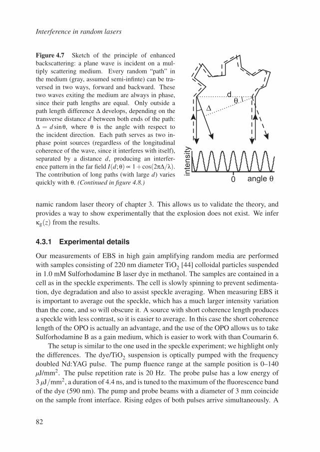
Interference in random lasers
Figure 4.7 Sketch of the principle of enhancedbackscattering: a plane wave is incident on a mul-tiply scattering medium. Every random “path” inthe medium (gray, assumed semi-infinte) can be tra-versed in two ways, forward and backward. Thesetwo waves exiting the medium are always in phase,since their path lengths are equal. Only outside apath length difference ∆ develops, depending on thetransverse distance d between both ends of the path:∆ = d sinθ, where θ is the angle with respect tothe incident direction. Each path serves as two in-phase point sources (regardless of the longitudinalcoherence of the wave, since it interferes with itself),separated by a distance d, producing an interfer-ence pattern in the far field I(d;θ) ∝ 1+cos(2π∆/λ).The contribution of long paths (with large d) variesquickly with θ. (Continued in figure 4.8.) 0
inte
nsity
angle θ
θd
∆
namic random laser theory of chapter 3. This allows us to validate the theory, andprovides a way to show experimentally that the explosion does not exist. We inferκg(z) from the results.
4.3.1 Experimental details
Our measurements of EBS in high gain amplifying random media are performedwith samples consisting of 220 nm diameter TiO2 [44] colloidal particles suspendedin 1.0 mM Sulforhodamine B laser dye in methanol. The samples are contained in acell as in the speckle experiments. The cell is slowly spinning to prevent sedimenta-tion, dye degradation and also to assist speckle averaging. When measuring EBS itis important to average out the speckle, which has a much larger intensity variationthan the cone, and so will obscure it. A source with short coherence length producesa speckle with less contrast, so it is easier to average. In this case the short coherencelength of the OPO is actually an advantage, and the use of the OPO allows us to takeSulforhodamine B as a gain medium, which is easier to work with than Coumarin 6.
The setup is similar to the one used in the speckle experiment; we highlight onlythe differences. The dye/TiO2 suspension is optically pumped with the frequencydoubled Nd:YAG pulse. The pump fluence range at the sample position is 0–140µJ/mm2. The pulse repetition rate is 20 Hz. The probe pulse has a low energy of3 µJ/mm2, a duration of 4.4 ns, and is tuned to the maximum of the fluorescence bandof the dye (590 nm). The pump and probe beams with a diameter of 3 mm coincideon the sample front interface. Rising edges of both pulses arrive simultaneously. A
82
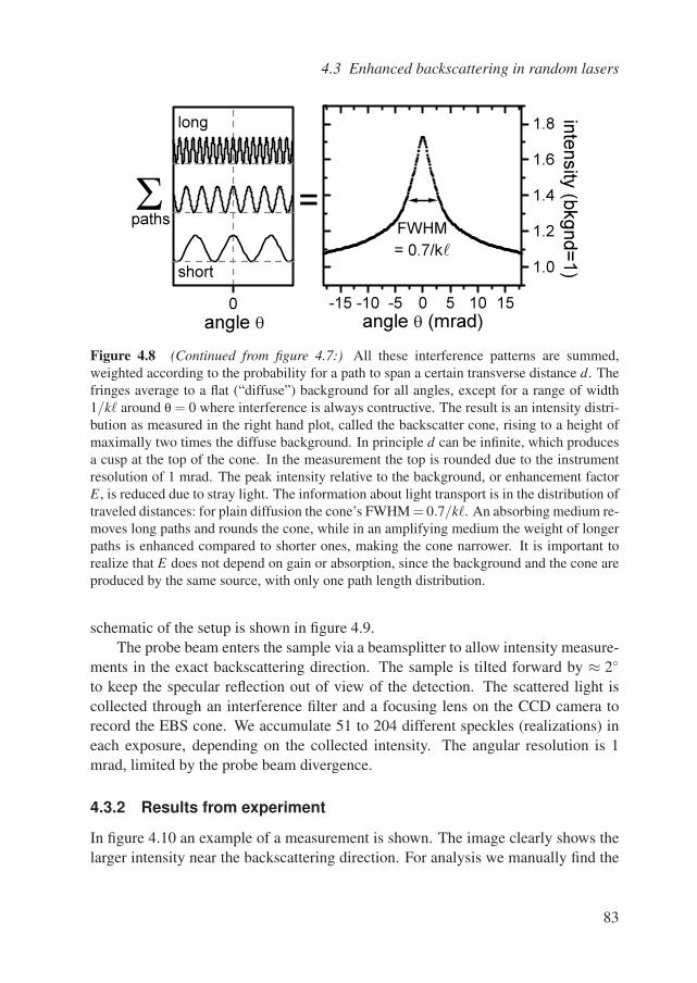
4.3 Enhanced backscattering in random lasers
0
short
long
angle -15 -10 -5 0 5 10 15
1.0
1.2
1.4
1.6
1.8
paths =
inte
nsity
(bkg
nd
=1
)
FWHM
= 0.7/k
angle (mrad)
Figure 4.8 (Continued from figure 4.7:) All these interference patterns are summed,weighted according to the probability for a path to span a certain transverse distance d. Thefringes average to a flat (“diffuse”) background for all angles, except for a range of width1/k around θ = 0 where interference is always contructive. The result is an intensity distri-bution as measured in the right hand plot, called the backscatter cone, rising to a height ofmaximally two times the diffuse background. In principle d can be infinite, which producesa cusp at the top of the cone. In the measurement the top is rounded due to the instrumentresolution of 1 mrad. The peak intensity relative to the background, or enhancement factorE, is reduced due to stray light. The information about light transport is in the distribution oftraveled distances: for plain diffusion the cone’s FWHM = 0.7/k. An absorbing medium re-moves long paths and rounds the cone, while in an amplifying medium the weight of longerpaths is enhanced compared to shorter ones, making the cone narrower. It is important torealize that E does not depend on gain or absorption, since the background and the cone areproduced by the same source, with only one path length distribution.
schematic of the setup is shown in figure 4.9.The probe beam enters the sample via a beamsplitter to allow intensity measure-
ments in the exact backscattering direction. The sample is tilted forward by ≈ 2
to keep the specular reflection out of view of the detection. The scattered light iscollected through an interference filter and a focusing lens on the CCD camera torecord the EBS cone. We accumulate 51 to 204 different speckles (realizations) ineach exposure, depending on the collected intensity. The angular resolution is 1mrad, limited by the probe beam divergence.
4.3.2 Results from experiment
In figure 4.10 an example of a measurement is shown. The image clearly shows thelarger intensity near the backscattering direction. For analysis we manually find the
83
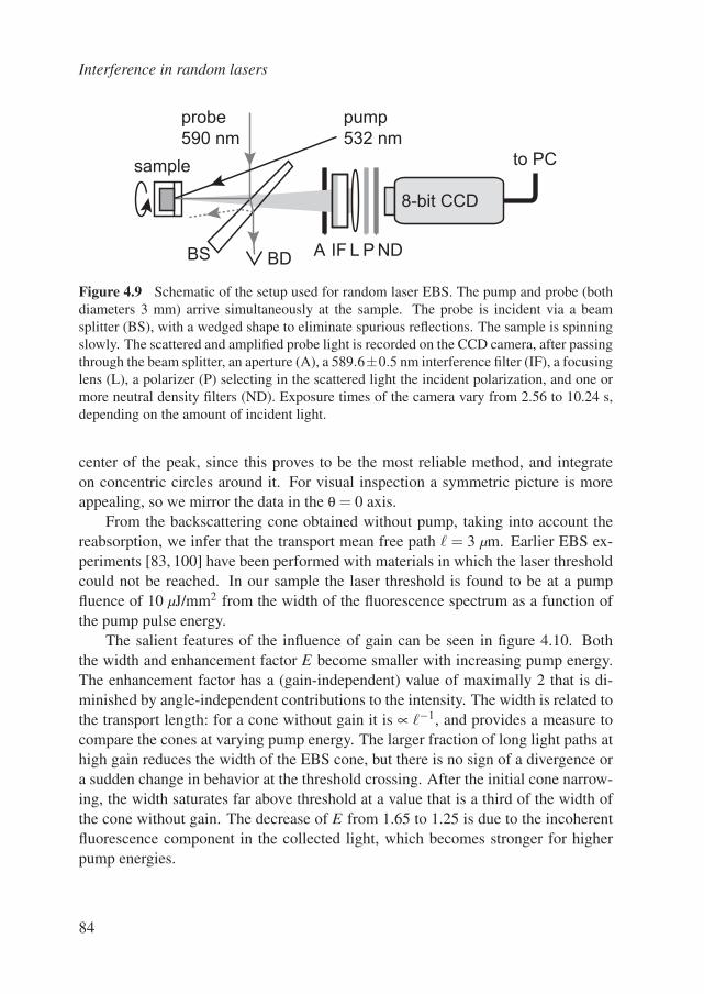
Interference in random lasers
A IF ND
8-bit CCD
to PC
PL
pump
532 nm
probe
590 nm
sample
BDBS
Figure 4.9 Schematic of the setup used for random laser EBS. The pump and probe (bothdiameters 3 mm) arrive simultaneously at the sample. The probe is incident via a beamsplitter (BS), with a wedged shape to eliminate spurious reflections. The sample is spinningslowly. The scattered and amplified probe light is recorded on the CCD camera, after passingthrough the beam splitter, an aperture (A), a 589.6±0.5 nm interference filter (IF), a focusinglens (L), a polarizer (P) selecting in the scattered light the incident polarization, and one ormore neutral density filters (ND). Exposure times of the camera vary from 2.56 to 10.24 s,depending on the amount of incident light.
center of the peak, since this proves to be the most reliable method, and integrateon concentric circles around it. For visual inspection a symmetric picture is moreappealing, so we mirror the data in the θ = 0 axis.
From the backscattering cone obtained without pump, taking into account thereabsorption, we infer that the transport mean free path = 3 µm. Earlier EBS ex-periments [83, 100] have been performed with materials in which the laser thresholdcould not be reached. In our sample the laser threshold is found to be at a pumpfluence of 10 µJ/mm2 from the width of the fluorescence spectrum as a function ofthe pump pulse energy.
The salient features of the influence of gain can be seen in figure 4.10. Boththe width and enhancement factor E become smaller with increasing pump energy.The enhancement factor has a (gain-independent) value of maximally 2 that is di-minished by angle-independent contributions to the intensity. The width is related tothe transport length: for a cone without gain it is ∝ −1, and provides a measure tocompare the cones at varying pump energy. The larger fraction of long light paths athigh gain reduces the width of the EBS cone, but there is no sign of a divergence ora sudden change in behavior at the threshold crossing. After the initial cone narrow-ing, the width saturates far above threshold at a value that is a third of the width ofthe cone without gain. The decrease of E from 1.65 to 1.25 is due to the incoherentfluorescence component in the collected light, which becomes stronger for higherpump energies.
84
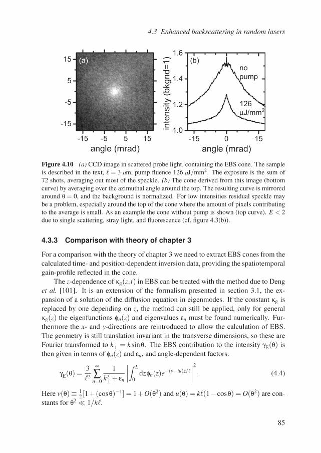
4.3 Enhanced backscattering in random lasers
(a) (b)no
pump
126
µJ/mm2
-15 0 151.0
1.2
1.4
1.6
inte
nsity
(bkgnd=
1)
angle (mrad)
-15 -5 5 15
-15
-5
5
15
angle (mrad)
Figure 4.10 (a) CCD image in scattered probe light, containing the EBS cone. The sampleis described in the text, = 3 µm, pump fluence 126 µJ/mm2. The exposure is the sum of72 shots, averaging out most of the speckle. (b) The cone derived from this image (bottomcurve) by averaging over the azimuthal angle around the top. The resulting curve is mirroredaround θ = 0, and the background is normalized. For low intensities residual speckle maybe a problem, especially around the top of the cone where the amount of pixels contributingto the average is small. As an example the cone without pump is shown (top curve). E < 2due to single scattering, stray light, and fluorescence (cf. figure 4.3(b)).
4.3.3 Comparison with theory of chapter 3
For a comparison with the theory of chapter 3 we need to extract EBS cones from thecalculated time- and position-dependent inversion data, providing the spatiotemporalgain-profile reflected in the cone.
The z-dependence of κg(z, t) in EBS can be treated with the method due to Denget al. [101]. It is an extension of the formalism presented in section 3.1, the ex-pansion of a solution of the diffusion equation in eigenmodes. If the constant κg isreplaced by one depending on z, the method can still be applied, only for generalκg(z) the eigenfunctions φn(z) and eigenvalues εn must be found numerically. Fur-thermore the x- and y-directions are reintroduced to allow the calculation of EBS.The geometry is still translation invariant in the transverse dimensions, so these areFourier transformed to k⊥ = k sinθ. The EBS contribution to the intensity γE(θ) isthen given in terms of φn(z) and εn, and angle-dependent factors:
γE(θ) =32
∞
∑n=0
1k2⊥ + εn
∣∣∣∣∫ L
0dzφn(z)e−(v−iu)z/
∣∣∣∣2
. (4.4)
Here v(θ)≡ 12 [1+(cosθ)−1] = 1+O(θ2) and u(θ) = k(1−cosθ) = O(θ2) are con-
stants for θ2 1/k.
85
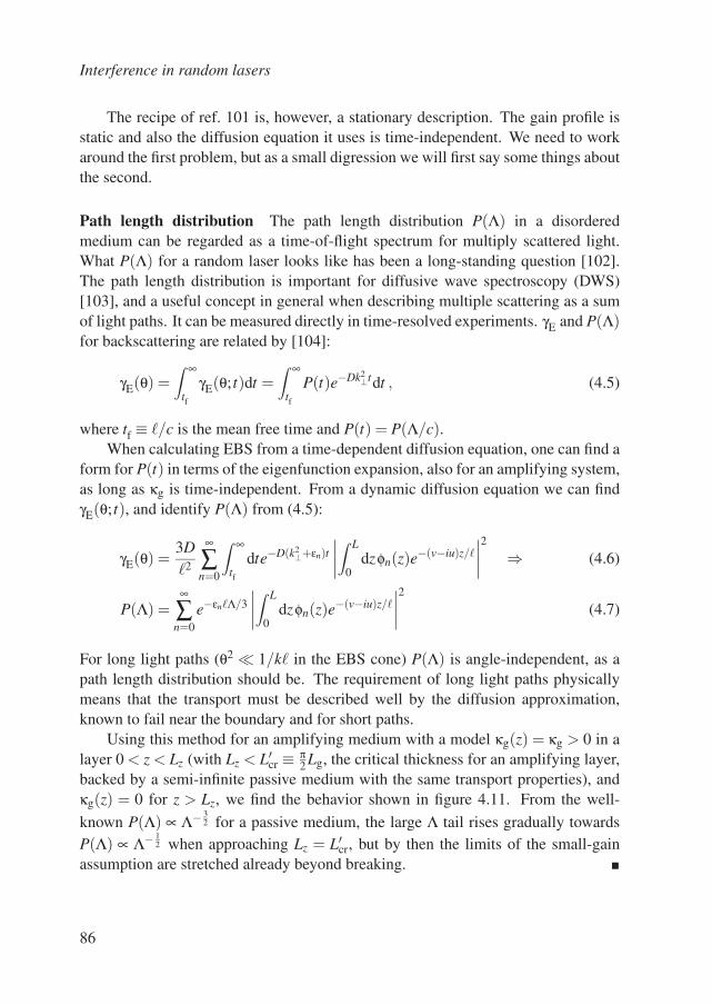
Interference in random lasers
The recipe of ref. 101 is, however, a stationary description. The gain profile isstatic and also the diffusion equation it uses is time-independent. We need to workaround the first problem, but as a small digression we will first say some things aboutthe second.
Path length distribution The path length distribution P(Λ) in a disorderedmedium can be regarded as a time-of-flight spectrum for multiply scattered light.What P(Λ) for a random laser looks like has been a long-standing question [102].The path length distribution is important for diffusive wave spectroscopy (DWS)[103], and a useful concept in general when describing multiple scattering as a sumof light paths. It can be measured directly in time-resolved experiments. γE and P(Λ)for backscattering are related by [104]:
γE(θ) =∫ ∞
tf
γE(θ; t)dt =∫ ∞
tf
P(t)e−Dk2⊥tdt , (4.5)
where tf ≡ /c is the mean free time and P(t) = P(Λ/c).When calculating EBS from a time-dependent diffusion equation, one can find a
form for P(t) in terms of the eigenfunction expansion, also for an amplifying system,as long as κg is time-independent. From a dynamic diffusion equation we can findγE(θ; t), and identify P(Λ) from (4.5):
γE(θ) =3D2
∞
∑n=0
∫ ∞
tf
dte−D(k2⊥+εn)t
∣∣∣∣∫ L
0dzφn(z)e−(v−iu)z/
∣∣∣∣2
⇒ (4.6)
P(Λ) =∞
∑n=0
e−εnΛ/3
∣∣∣∣∫ L
0dzφn(z)e−(v−iu)z/
∣∣∣∣2
(4.7)
For long light paths (θ2 1/k in the EBS cone) P(Λ) is angle-independent, as apath length distribution should be. The requirement of long light paths physicallymeans that the transport must be described well by the diffusion approximation,known to fail near the boundary and for short paths.
Using this method for an amplifying medium with a model κg(z) = κg > 0 in alayer 0 < z < Lz (with Lz < L′
cr ≡ π2 Lg, the critical thickness for an amplifying layer,
backed by a semi-infinite passive medium with the same transport properties), andκg(z) = 0 for z > Lz, we find the behavior shown in figure 4.11. From the well-
known P(Λ) ∝ Λ− 32 for a passive medium, the large Λ tail rises gradually towards
P(Λ) ∝ Λ− 12 when approaching Lz = L′
cr, but by then the limits of the small-gainassumption are stretched already beyond breaking.
86
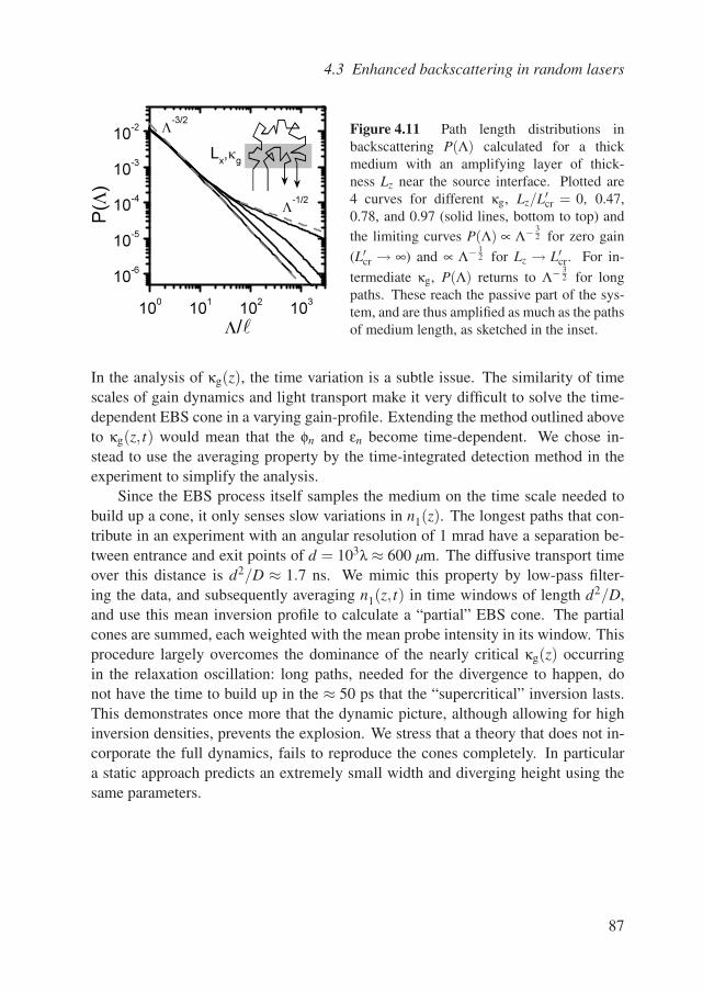
4.3 Enhanced backscattering in random lasers
100
101
102
103
10-6
10-5
10-4
10-3
10-2
Lx,
g
-1/2
-3/2
P(
)
/
Figure 4.11 Path length distributions inbackscattering P(Λ) calculated for a thickmedium with an amplifying layer of thick-ness Lz near the source interface. Plotted are4 curves for different κg, Lz/L′
cr = 0, 0.47,0.78, and 0.97 (solid lines, bottom to top) andthe limiting curves P(Λ) ∝ Λ− 3
2 for zero gain(L′
cr → ∞) and ∝ Λ− 12 for Lz → L′
cr. For in-termediate κg, P(Λ) returns to Λ− 3
2 for longpaths. These reach the passive part of the sys-tem, and are thus amplified as much as the pathsof medium length, as sketched in the inset.
In the analysis of κg(z), the time variation is a subtle issue. The similarity of timescales of gain dynamics and light transport make it very difficult to solve the time-dependent EBS cone in a varying gain-profile. Extending the method outlined aboveto κg(z, t) would mean that the φn and εn become time-dependent. We chose in-stead to use the averaging property by the time-integrated detection method in theexperiment to simplify the analysis.
Since the EBS process itself samples the medium on the time scale needed tobuild up a cone, it only senses slow variations in n1(z). The longest paths that con-tribute in an experiment with an angular resolution of 1 mrad have a separation be-tween entrance and exit points of d = 103λ ≈ 600 µm. The diffusive transport timeover this distance is d2/D ≈ 1.7 ns. We mimic this property by low-pass filter-ing the data, and subsequently averaging n1(z, t) in time windows of length d2/D,and use this mean inversion profile to calculate a “partial” EBS cone. The partialcones are summed, each weighted with the mean probe intensity in its window. Thisprocedure largely overcomes the dominance of the nearly critical κg(z) occurringin the relaxation oscillation: long paths, needed for the divergence to happen, donot have the time to build up in the ≈ 50 ps that the “supercritical” inversion lasts.This demonstrates once more that the dynamic picture, although allowing for highinversion densities, prevents the explosion. We stress that a theory that does not in-corporate the full dynamics, fails to reproduce the cones completely. In particulara static approach predicts an extremely small width and diverging height using thesame parameters.
87
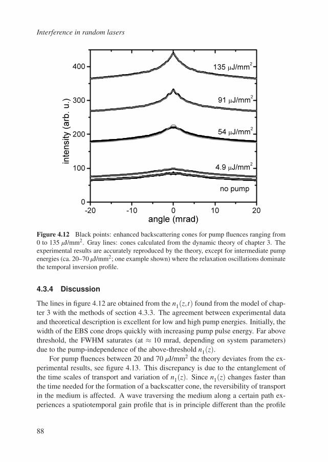
Interference in random lasers
-20 -10 0 10 200
100
200
300
400
no pump
inte
nsity (
arb
. u.)
angle (mrad)
135 J/mm2
91 J/mm2
54 J/mm2
4.9 J/mm2
Figure 4.12 Black points: enhanced backscattering cones for pump fluences ranging from0 to 135 µJ/mm2. Gray lines: cones calculated from the dynamic theory of chapter 3. Theexperimental results are accurately reproduced by the theory, except for intermediate pumpenergies (ca. 20–70 µJ/mm2; one example shown) where the relaxation oscillations dominatethe temporal inversion profile.
4.3.4 Discussion
The lines in figure 4.12 are obtained from the n1(z, t) found from the model of chap-ter 3 with the methods of section 4.3.3. The agreement between experimental dataand theoretical description is excellent for low and high pump energies. Initially, thewidth of the EBS cone drops quickly with increasing pump pulse energy. Far abovethreshold, the FWHM saturates (at ≈ 10 mrad, depending on system parameters)due to the pump-independence of the above-threshold n1(z).
For pump fluences between 20 and 70 µJ/mm2 the theory deviates from the ex-perimental results, see figure 4.13. This discrepancy is due to the entanglement ofthe time scales of transport and variation of n1(z). Since n1(z) changes faster thanthe time needed for the formation of a backscatter cone, the reversibility of transportin the medium is affected. A wave traversing the medium along a certain path ex-periences a spatiotemporal gain profile that is in principle different than the profile
88
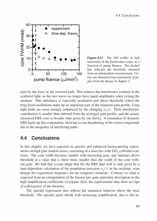
4.4 Conclusions
0 50 100 1500
10
20
30
40 experiment
time-dep. theory
cone F
WH
M (
mra
d)
pump fluence (J/mm2
)
Figure 4.13 The full widths at halfmaximum of the backscatter cones as afunction of pump fluence. The dashedline indicates the threshold, obtainedfrom an independent measurement. Cir-cles are obtained from experiment, trian-gles from the theory in chapter 3.
seen by the wave in the reversed path. This reduces the interference contrast in thescattered light, as the two waves no longer have equal amplitudes when exiting themedium. This unbalance is especially prominent just above threshold, where thelong-lived oscillations make up an important part of the temporal gain profile. Longlight paths are most strongly influenced by the changing n1(z). Their interferencecontribution is smaller than inferred from the averaged gain profile, and the actual,measured EBS cone is broader than given by our theory. A simulation of dynamicEBS backs up this explanation, showing a cone broadening of the correct magnitudedue to the inequality of interfering paths.
4.4 Conclusions
In this chapter, we have reported on speckle and enhanced backscattering experi-ments on high gain random lasers, consisting of a laser dye with TiO2 colloidal scat-terers. The cone width becomes smaller with increasing gain, and saturates abovethreshold at a value that is three times smaller than the width of the cone with-out gain. We find that a cone shape that fits the EBS data well is only given by atime-dependent calculation of the population inversion n1(z) in the medium, eventhough the experiment integrates out the temporal variations. Contrary to what isexpected from an extrapolation of the known low-gain stationary description to thehigh amplification coefficients of organic dyes, the experimental data show no signof a divergence of the intensity.
The speckle experiment also reflects the saturation behavior above the laserthreshold. The speckle spots shrink with increasing amplification, due to the in-
89
Interference in random lasers
creased contribution of long light paths. This trend, too, saturates far above thresh-old, where the speckles have a constant angular size of 1.5 times smaller than thespeckles from a passive sample. The speckle retains its Rayleigh intensity statistics.The analysis of the speckle autocorrelation in terms of a coherent amplified probeon an incoherent fluorescence background is consistent.
These results show that the spatial gain profile can be investigated well withprobing techniques, allowing a quantitative study of light transport in random lasers.The theory developed in chapter 3 is validated by these measurements, and the inter-pretation of experimental data with the help of comparisons with that theory providesinsight in the actual dynamics of a random laser, even by the stationary experimentsreported here.
90
5.Narrow peaks in fluorescence
from scattering systems
Recently, several articles have appeared reporting on the observation and interpre-tation of narrow peaks in the emission spectrum of random lasers. The phenomenonwas said to be a manifestation of Anderson localization. This is a bold claim,needing a solid experimental backing. We performed a series of experiments tryingto replicate the results and to investigate these peaks more quantitatively andsystematically than in the published research. The outcome of our experiments canbe explained in terms of material properties, and we assert that this explanation canbe generalized to the literature results.
The combination of Anderson localization and amplification has been appealingsince the idea was brought up [71]. The picturesque view of Anderson localizedlight being captured in “loops” suggests the possibility of random ring laser cavi-ties [52, 105], providing resonant feedback, i.e. light experiences a phase shift of aninteger times 2π in a round trip. This would permit a “coherent random laser”, a third,qualitatively different regime in scattering amplifying systems (first and second be-ing the single, post-ASE scattering as in section 2.3.2, and multiple scattering as inthe other experiments described in this thesis). The suggestion that Anderson local-ization might be facilitated by the presence of gain—localization being destroyedby absorption, and gain being negative absorption, in a way—has been present for along time, but up to today nobody has theoretically pursued the idea to its full (3D)extent.
Experimentalists have put a tremendous amount of effort into achieving local-ization of light, until now without undisputed success. Furthermore, the knowledgeabout the phenomenology of the localized state in an actual measurement is very lim-ited. These considerations call for wariness when interpreting experimental resultsin terms of Anderson localization. Fluorescence is sensitive to microscopic changes
91
Narrow peaks in fluorescence from scattering systems
in the electronic structure of the sample (e.g. specific defects, surface adsorption).For this reason material parameters should only be ruled out as an explanation for aspectroscopic phenomenon after very careful inspection.
5.1 Critical review
5.1.1 Observations and interpretations from the literature
In this section we present an overview of relevant results and interpretations fromthe literature, followed by a discussion. The reported phenomena are summarizedin figure 5.1: sharp peaks appear in the emission spectrum of a random laser, ontop of the narrowing ASE spectrum, near the maximum of the emission spectrum.Such observations have been made in multiply scattering samples made of ZnO andGaN powders [52, 106–110], and dye solutions with ZnO scatterers [53], but also intransparent samples, such as thin films of nanocrystalline ZnO [105, 110–113], dye-doped gel, active polymer, or index-matched opal [114, 115]. A distinction has tobe made between the multiply scattering materials and thin films, that have becomepart of the same discussion. The observations are similar for both types of samples,although the optical properties differ strongly.
The measurements have been explained in terms of resonant feedback inducedby disorder. A dominant idea is that of microscopic ring cavities, light trajectoriesthat return to the same scatterer with a round trip phase lag of n ·2π, with n an integer.Recurrent scattering events (loop paths of any length) have been shown to exist asa single-scattering-like contribution to the backscattered intensity [116] for k 10.We will discuss this interpretation in some more detail in section 5.1.2.
Recently some results were reinterpreted [108] in terms of the system’s electro-magnetic eigenstates, characterized by a spectral width δω and a spacing Ω. Theeigenmodes overlap in frequency, δω > Ω, for less than very strong disorder—saidto result in the incoherent-feedback multimode random laser as in our chapter 2—todecouple for strong disorder, δω < Ω—allowing a coherent random laser working ina single electromagnetic mode of the system. See also our discussion of the randomlaser vs. cavity laser β-factor, section 3.3.1. δω/Ω < 1 for the transport eigenstatesof a disordered medium is the Thouless criterion for Anderson localization [88], im-plying that a random laser exhibiting the narrow peaks should be in the localizedregime.
To substantiate the proposal of a disorder-induced resonant feedback, one hasattempted to reduce the amount of disorder and so make the effect disappear. Onemethod is already mentioned in figure 5.1: to change the amount of scatterers in thedye solution, which indeed has an effect on the occurrence of the frequency peaks.
92
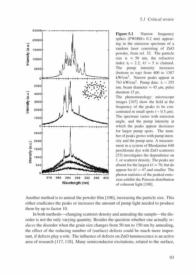
5.1 Critical review
Figure 5.1 Narrow frequencyspikes (FWHM≈ 0.2 nm) appear-ing in the emission spectrum of arandom laser consisting of ZnOpowder, from ref. 52. The particlesize is ≈ 50 nm, the refractiveindex η = 2.2; k = 5 is claimed.The pump intensity increases(bottom to top) from 400 to 1387kW/cm2. Narrow peaks appear at763 kW/cm2. Pump data: λ = 355nm, beam diameter ≈ 45 µm, pulseduration 15 ps.The phenomenology: microscopeimages [107] show the field at thefrequency of the peaks to be con-centrated in small spots (∼ 0.5 µm).The spectrum varies with emissionangle, and the pump intensity atwhich the peaks appear decreasesfor larger pump spots. The num-ber of peaks grows with pump inten-sity and the pump area. A measure-ment in a system of Rhodamine 640perchlorate dye with ZnO scatterers[53] investigates the dependence on, or scatterer density. The peaks areabsent for the largest k≈ 70, but doappear for k = 47 and smaller. Thephoton statistics of the peaked emis-sion exhibit the Poisson distributionof coherent light [108].
Another method is to anneal the powder film [106], increasing the particle size. Thiseither eradicates the peaks or increases the amount of pump light needed to producethem by up to factor 10.
In both methods—changing scatterer density and annealing the sample—the dis-order is not the only varying quantity. Besides the question whether one actually re-duces the disorder when the grain size changes from 50 nm to 150 nm by annealing,the effect of the reducing number of (surface) defects could be much more impor-tant, if defects play a role. The influence of defects on ZnO luminescence is an activearea of research [117, 118]. Many semiconductor excitations, related to the surface,
93
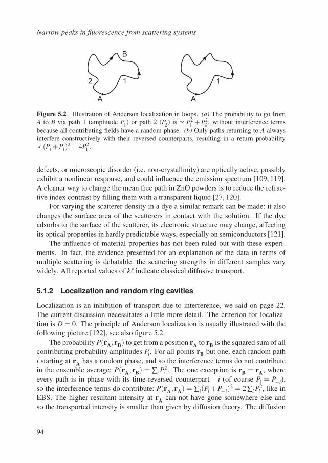
Narrow peaks in fluorescence from scattering systems
A
B
12
A
1
Figure 5.2 Illustration of Anderson localization in loops. (a) The probability to go fromA to B via path 1 (amplitude P1) or path 2 (P2) is ∝ P2
1 + P22 , without interference terms
because all contributing fields have a random phase. (b) Only paths returning to A alwaysinterfere constructively with their reversed counterparts, resulting in a return probability∝ (P1 +P1)
2 = 4P21 .
defects, or microscopic disorder (i.e. non-crystallinity) are optically active, possiblyexhibit a nonlinear response, and could influence the emission spectrum [109, 119].A cleaner way to change the mean free path in ZnO powders is to reduce the refrac-tive index contrast by filling them with a transparent liquid [27, 120].
For varying the scatterer density in a dye a similar remark can be made: it alsochanges the surface area of the scatterers in contact with the solution. If the dyeadsorbs to the surface of the scatterer, its electronic structure may change, affectingits optical properties in hardly predictable ways, especially on semiconductors [121].
The influence of material properties has not been ruled out with these experi-ments. In fact, the evidence presented for an explanation of the data in terms ofmultiple scattering is debatable: the scattering strengths in different samples varywidely. All reported values of k indicate classical diffusive transport.
5.1.2 Localization and random ring cavities
Localization is an inhibition of transport due to interference, we said on page 22.The current discussion necessitates a little more detail. The criterion for localiza-tion is D = 0. The principle of Anderson localization is usually illustrated with thefollowing picture [122], see also figure 5.2.
The probability P(rA,rB) to get from a position rA to rB is the squared sum of allcontributing probability amplitudes Pi. For all points rB but one, each random pathi starting at rA has a random phase, and so the interference terms do not contributein the ensemble average; P(rA,rB) = ∑i P2
i . The one exception is rB = rA, whereevery path is in phase with its time-reversed counterpart −i (of course Pi = P−i),so the interference terms do contribute: P(rA,rA) = ∑i(Pi + P−i)
2 = 2∑i P2i , like in
EBS. The higher resultant intensity at rA can not have gone somewhere else andso the transported intensity is smaller than given by diffusion theory. The diffusion
94
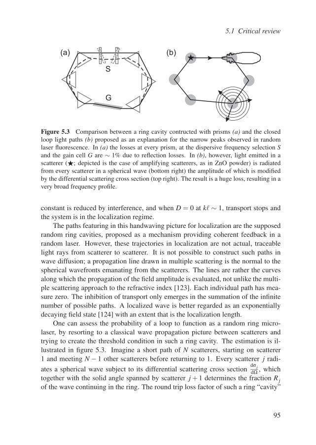
5.1 Critical review
G
(a) (b)
S
Figure 5.3 Comparison between a ring cavity contructed with prisms (a) and the closedloop light paths (b) proposed as an explanation for the narrow peaks observed in randomlaser fluorescence. In (a) the losses at every prism, at the dispersive frequency selection Sand the gain cell G are ∼ 1% due to reflection losses. In (b), however, light emitted in ascatterer (; depicted is the case of amplifying scatterers, as in ZnO powder) is radiatedfrom every scatterer in a spherical wave (bottom right) the amplitude of which is modifiedby the differential scattering cross section (top right). The result is a huge loss, resulting in avery broad frequency profile.
constant is reduced by interference, and when D = 0 at k ∼ 1, transport stops andthe system is in the localization regime.
The paths featuring in this handwaving picture for localization are the supposedrandom ring cavities, proposed as a mechanism providing coherent feedback in arandom laser. However, these trajectories in localization are not actual, traceablelight rays from scatterer to scatterer. It is not possible to construct such paths inwave diffusion; a propagation line drawn in multiple scattering is the normal to thespherical wavefronts emanating from the scatterers. The lines are rather the curvesalong which the propagation of the field amplitude is evaluated, not unlike the multi-ple scattering approach to the refractive index [123]. Each individual path has mea-sure zero. The inhibition of transport only emerges in the summation of the infinitenumber of possible paths. A localized wave is better regarded as an exponentiallydecaying field state [124] with an extent that is the localization length.
One can assess the probability of a loop to function as a random ring micro-laser, by resorting to a classical wave propagation picture between scatterers andtrying to create the threshold condition in such a ring cavity. The estimation is il-lustrated in figure 5.3. Imagine a short path of N scatterers, starting on scatterer1 and meeting N − 1 other scatterers before returning to 1. Every scatterer j radi-
ates a spherical wave subject to its differential scattering cross sectiondσ j
dΩ , whichtogether with the solid angle spanned by scatterer j + 1 determines the fraction R jof the wave continuing in the ring. The round trip loss factor of such a ring “cavity”
95
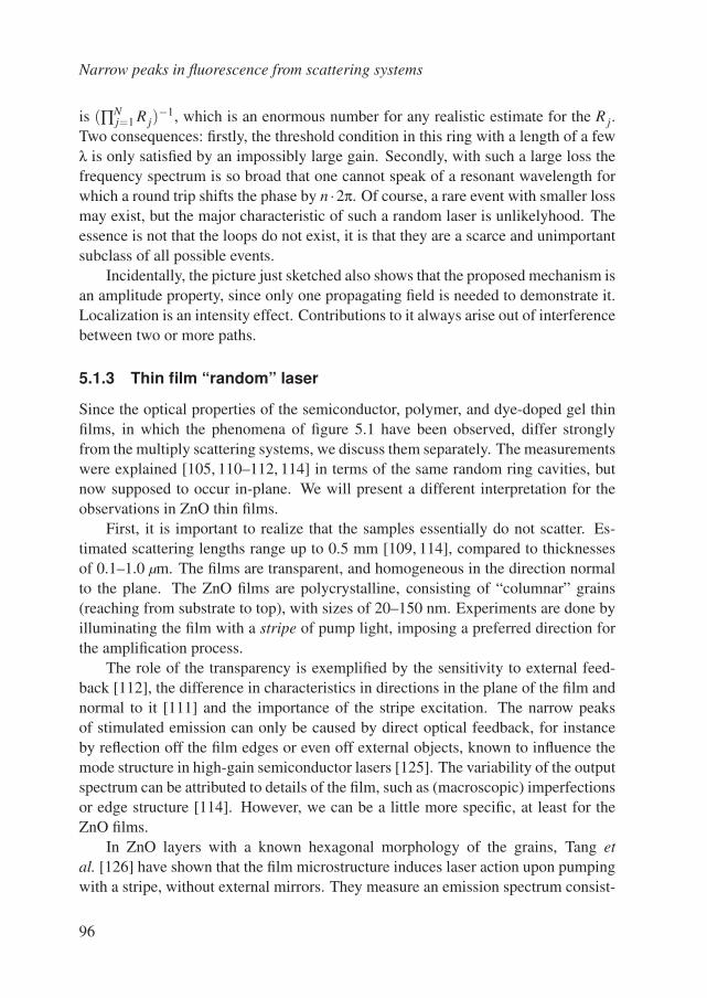
Narrow peaks in fluorescence from scattering systems
is (∏Nj=1 R j)
−1, which is an enormous number for any realistic estimate for the R j.Two consequences: firstly, the threshold condition in this ring with a length of a fewλ is only satisfied by an impossibly large gain. Secondly, with such a large loss thefrequency spectrum is so broad that one cannot speak of a resonant wavelength forwhich a round trip shifts the phase by n ·2π. Of course, a rare event with smaller lossmay exist, but the major characteristic of such a random laser is unlikelyhood. Theessence is not that the loops do not exist, it is that they are a scarce and unimportantsubclass of all possible events.
Incidentally, the picture just sketched also shows that the proposed mechanism isan amplitude property, since only one propagating field is needed to demonstrate it.Localization is an intensity effect. Contributions to it always arise out of interferencebetween two or more paths.
5.1.3 Thin film “random” laser
Since the optical properties of the semiconductor, polymer, and dye-doped gel thinfilms, in which the phenomena of figure 5.1 have been observed, differ stronglyfrom the multiply scattering systems, we discuss them separately. The measurementswere explained [105, 110–112, 114] in terms of the same random ring cavities, butnow supposed to occur in-plane. We will present a different interpretation for theobservations in ZnO thin films.
First, it is important to realize that the samples essentially do not scatter. Es-timated scattering lengths range up to 0.5 mm [109, 114], compared to thicknessesof 0.1–1.0 µm. The films are transparent, and homogeneous in the direction normalto the plane. The ZnO films are polycrystalline, consisting of “columnar” grains(reaching from substrate to top), with sizes of 20–150 nm. Experiments are done byilluminating the film with a stripe of pump light, imposing a preferred direction forthe amplification process.
The role of the transparency is exemplified by the sensitivity to external feed-back [112], the difference in characteristics in directions in the plane of the film andnormal to it [111] and the importance of the stripe excitation. The narrow peaksof stimulated emission can only be caused by direct optical feedback, for instanceby reflection off the film edges or even off external objects, known to influence themode structure in high-gain semiconductor lasers [125]. The variability of the outputspectrum can be attributed to details of the film, such as (macroscopic) imperfectionsor edge structure [114]. However, we can be a little more specific, at least for theZnO films.
In ZnO layers with a known hexagonal morphology of the grains, Tang etal. [126] have shown that the film microstructure induces laser action upon pumpingwith a stripe, without external mirrors. They measure an emission spectrum consist-
96
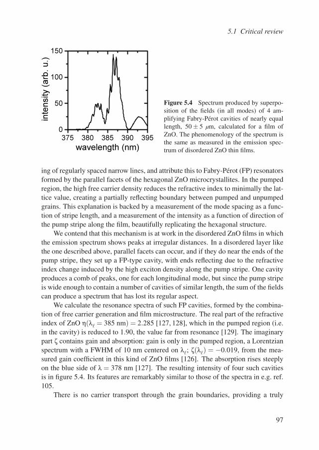
5.1 Critical review
375 380 385 390 395
0
50
100
150
wavelength (nm)
inte
nsity (
arb
. u.)
Figure 5.4 Spectrum produced by superpo-sition of the fields (in all modes) of 4 am-plifying Fabry-Perot cavities of nearly equallength, 50 ± 5 µm, calculated for a film ofZnO. The phenomenology of the spectrum isthe same as measured in the emission spec-trum of disordered ZnO thin films.
ing of regularly spaced narrow lines, and attribute this to Fabry-Perot (FP) resonatorsformed by the parallel facets of the hexagonal ZnO microcrystallites. In the pumpedregion, the high free carrier density reduces the refractive index to minimally the lat-tice value, creating a partially reflecting boundary between pumped and unpumpedgrains. This explanation is backed by a measurement of the mode spacing as a func-tion of stripe length, and a measurement of the intensity as a function of direction ofthe pump stripe along the film, beautifully replicating the hexagonal structure.
We contend that this mechanism is at work in the disordered ZnO films in whichthe emission spectrum shows peaks at irregular distances. In a disordered layer likethe one described above, parallel facets can occur, and if they do near the ends of thepump stripe, they set up a FP-type cavity, with ends reflecting due to the refractiveindex change induced by the high exciton density along the pump stripe. One cavityproduces a comb of peaks, one for each longitudinal mode, but since the pump stripeis wide enough to contain a number of cavities of similar length, the sum of the fieldscan produce a spectrum that has lost its regular aspect.
We calculate the resonance spectra of such FP cavities, formed by the combina-tion of free carrier generation and film microstructure. The real part of the refractiveindex of ZnO η(λ = 385 nm) = 2.285 [127, 128], which in the pumped region (i.e.in the cavity) is reduced to 1.90, the value far from resonance [129]. The imaginarypart ζ contains gain and absorption: gain is only in the pumped region, a Lorentzianspectrum with a FWHM of 10 nm centered on λ; ζ(λ) = −0.019, from the mea-sured gain coefficient in this kind of ZnO films [126]. The absorption rises steeplyon the blue side of λ = 378 nm [127]. The resulting intensity of four such cavitiesis in figure 5.4. Its features are remarkably similar to those of the spectra in e.g. ref.105.
There is no carrier transport through the grain boundaries, providing a truly
97
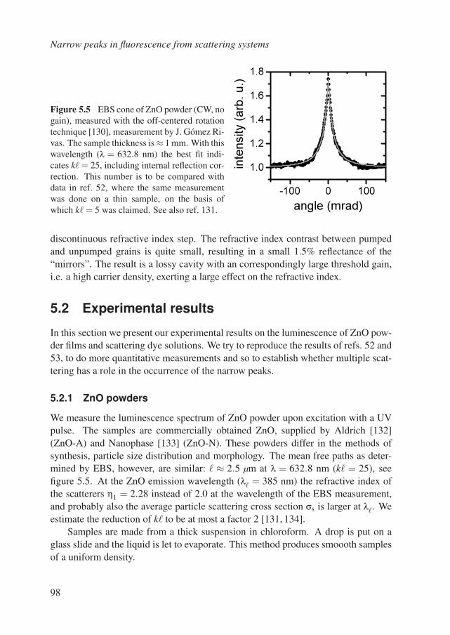
Narrow peaks in fluorescence from scattering systems
Figure 5.5 EBS cone of ZnO powder (CW, nogain), measured with the off-centered rotationtechnique [130], measurement by J. Gomez Ri-vas. The sample thickness is ≈ 1 mm. With thiswavelength (λ = 632.8 nm) the best fit indi-cates k = 25, including internal reflection cor-rection. This number is to be compared withdata in ref. 52, where the same measurementwas done on a thin sample, on the basis ofwhich k = 5 was claimed. See also ref. 131.
-100 0 100
1.0
1.2
1.4
1.6
1.8
inte
nsity (
arb
. u.)
angle (mrad)
discontinuous refractive index step. The refractive index contrast between pumpedand unpumped grains is quite small, resulting in a small 1.5% reflectance of the“mirrors”. The result is a lossy cavity with an correspondingly large threshold gain,i.e. a high carrier density, exerting a large effect on the refractive index.
5.2 Experimental results
In this section we present our experimental results on the luminescence of ZnO pow-der films and scattering dye solutions. We try to reproduce the results of refs. 52 and53, to do more quantitative measurements and so to establish whether multiple scat-tering has a role in the occurrence of the narrow peaks.
5.2.1 ZnO powders
We measure the luminescence spectrum of ZnO powder upon excitation with a UVpulse. The samples are commercially obtained ZnO, supplied by Aldrich [132](ZnO-A) and Nanophase [133] (ZnO-N). These powders differ in the methods ofsynthesis, particle size distribution and morphology. The mean free paths as deter-mined by EBS, however, are similar: ≈ 2.5 µm at λ = 632.8 nm (k = 25), seefigure 5.5. At the ZnO emission wavelength (λ = 385 nm) the refractive index ofthe scatterers η1 = 2.28 instead of 2.0 at the wavelength of the EBS measurement,and probably also the average particle scattering cross section σs is larger at λ. Weestimate the reduction of k to be at most a factor 2 [131, 134].
Samples are made from a thick suspension in chloroform. A drop is put on aglass slide and the liquid is let to evaporate. This method produces smoooth samplesof a uniform density.
98
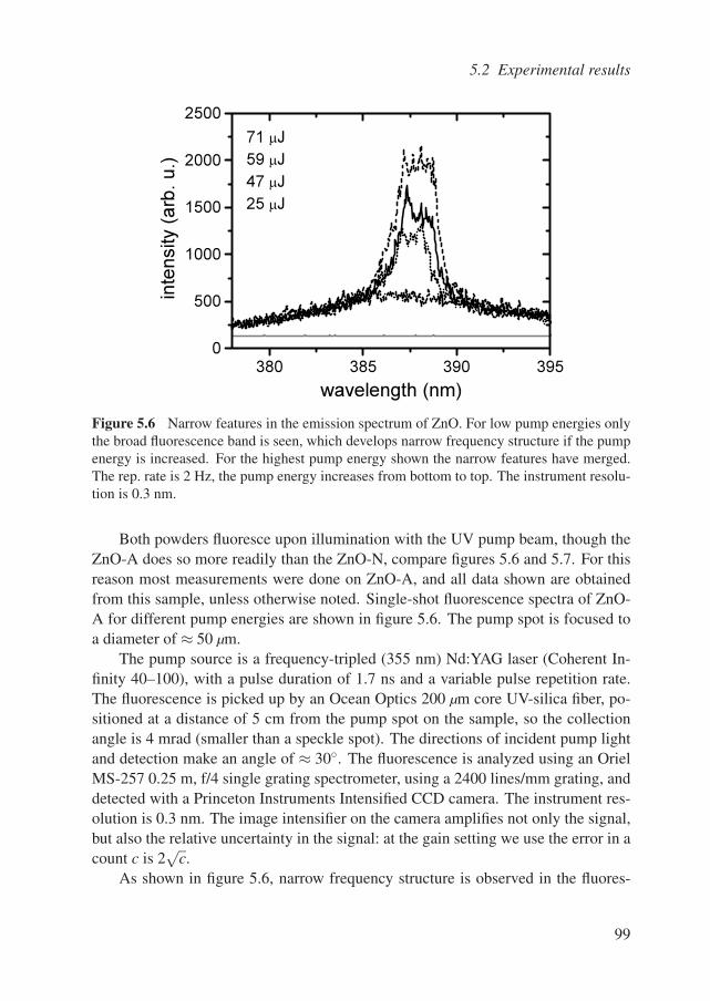
5.2 Experimental results
380 385 390 395
0
500
1000
1500
2000
2500
71 J
59 J
47 J
25 J
wavelength (nm)
inte
nsity (
arb
. u.)
Figure 5.6 Narrow features in the emission spectrum of ZnO. For low pump energies onlythe broad fluorescence band is seen, which develops narrow frequency structure if the pumpenergy is increased. For the highest pump energy shown the narrow features have merged.The rep. rate is 2 Hz, the pump energy increases from bottom to top. The instrument resolu-tion is 0.3 nm.
Both powders fluoresce upon illumination with the UV pump beam, though theZnO-A does so more readily than the ZnO-N, compare figures 5.6 and 5.7. For thisreason most measurements were done on ZnO-A, and all data shown are obtainedfrom this sample, unless otherwise noted. Single-shot fluorescence spectra of ZnO-A for different pump energies are shown in figure 5.6. The pump spot is focused toa diameter of ≈ 50 µm.
The pump source is a frequency-tripled (355 nm) Nd:YAG laser (Coherent In-finity 40–100), with a pulse duration of 1.7 ns and a variable pulse repetition rate.The fluorescence is picked up by an Ocean Optics 200 µm core UV-silica fiber, po-sitioned at a distance of 5 cm from the pump spot on the sample, so the collectionangle is 4 mrad (smaller than a speckle spot). The directions of incident pump lightand detection make an angle of ≈ 30. The fluorescence is analyzed using an OrielMS-257 0.25 m, f/4 single grating spectrometer, using a 2400 lines/mm grating, anddetected with a Princeton Instruments Intensified CCD camera. The instrument res-olution is 0.3 nm. The image intensifier on the camera amplifies not only the signal,but also the relative uncertainty in the signal: at the gain setting we use the error in acount c is 2
√c.
As shown in figure 5.6, narrow frequency structure is observed in the fluores-
99
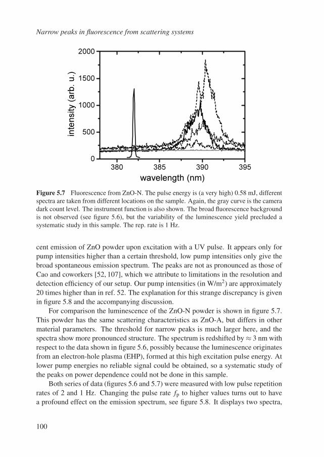
Narrow peaks in fluorescence from scattering systems
380 385 390 395
0
500
1000
1500
2000
inte
nsity (
arb
. u.)
wavelength (nm)
Figure 5.7 Fluorescence from ZnO-N. The pulse energy is (a very high) 0.58 mJ, differentspectra are taken from different locations on the sample. Again, the gray curve is the cameradark count level. The instrument function is also shown. The broad fluorescence backgroundis not observed (see figure 5.6), but the variability of the luminescence yield precluded asystematic study in this sample. The rep. rate is 1 Hz.
cent emission of ZnO powder upon excitation with a UV pulse. It appears only forpump intensities higher than a certain threshold, low pump intensities only give thebroad spontaneous emission spectrum. The peaks are not as pronounced as those ofCao and coworkers [52, 107], which we attribute to limitations in the resolution anddetection efficiency of our setup. Our pump intensities (in W/m2) are approximately20 times higher than in ref. 52. The explanation for this strange discrepancy is givenin figure 5.8 and the accompanying discussion.
For comparison the luminescence of the ZnO-N powder is shown in figure 5.7.This powder has the same scattering characteristics as ZnO-A, but differs in othermaterial parameters. The threshold for narrow peaks is much larger here, and thespectra show more pronounced structure. The spectrum is redshifted by ≈ 3 nm withrespect to the data shown in figure 5.6, possibly because the luminescence originatesfrom an electron-hole plasma (EHP), formed at this high excitation pulse energy. Atlower pump energies no reliable signal could be obtained, so a systematic study ofthe peaks on power dependence could not be done in this sample.
Both series of data (figures 5.6 and 5.7) were measured with low pulse repetitionrates of 2 and 1 Hz. Changing the pulse rate fp to higher values turns out to havea profound effect on the emission spectrum, see figure 5.8. It displays two spectra,
100
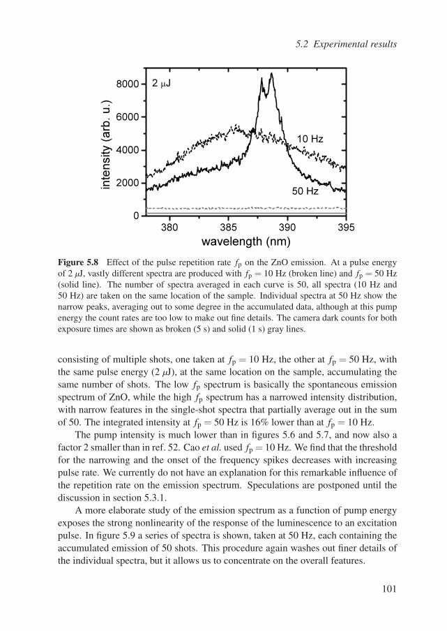
5.2 Experimental results
380 385 390 395
0
2000
4000
6000
8000 2 J
wavelength (nm)
inte
nsity (
arb
. u.)
50 Hz
10 Hz
Figure 5.8 Effect of the pulse repetition rate fp on the ZnO emission. At a pulse energyof 2 µJ, vastly different spectra are produced with fp = 10 Hz (broken line) and fp = 50 Hz(solid line). The number of spectra averaged in each curve is 50, all spectra (10 Hz and50 Hz) are taken on the same location of the sample. Individual spectra at 50 Hz show thenarrow peaks, averaging out to some degree in the accumulated data, although at this pumpenergy the count rates are too low to make out fine details. The camera dark counts for bothexposure times are shown as broken (5 s) and solid (1 s) gray lines.
consisting of multiple shots, one taken at fp = 10 Hz, the other at fp = 50 Hz, withthe same pulse energy (2 µJ), at the same location on the sample, accumulating thesame number of shots. The low fp spectrum is basically the spontaneous emissionspectrum of ZnO, while the high fp spectrum has a narrowed intensity distribution,with narrow features in the single-shot spectra that partially average out in the sumof 50. The integrated intensity at fp = 50 Hz is 16% lower than at fp = 10 Hz.
The pump intensity is much lower than in figures 5.6 and 5.7, and now also afactor 2 smaller than in ref. 52. Cao et al. used fp = 10 Hz. We find that the thresholdfor the narrowing and the onset of the frequency spikes decreases with increasingpulse rate. We currently do not have an explanation for this remarkable influence ofthe repetition rate on the emission spectrum. Speculations are postponed until thediscussion in section 5.3.1.
A more elaborate study of the emission spectrum as a function of pump energyexposes the strong nonlinearity of the response of the luminescence to an excitationpulse. In figure 5.9 a series of spectra is shown, taken at 50 Hz, each containing theaccumulated emission of 50 shots. This procedure again washes out finer details ofthe individual spectra, but it allows us to concentrate on the overall features.
101
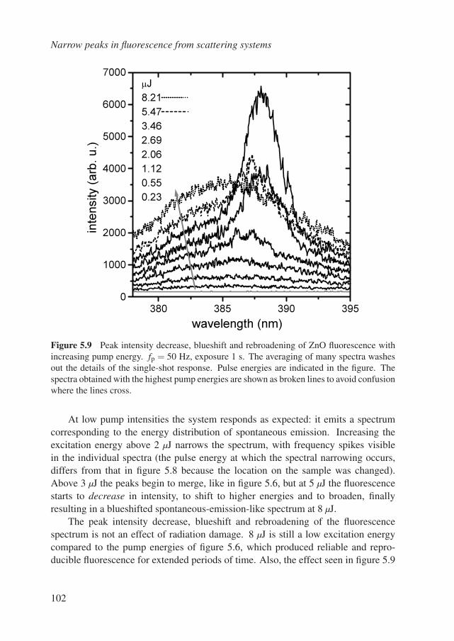
Narrow peaks in fluorescence from scattering systems
380 385 390 395
0
1000
2000
3000
4000
5000
6000
7000
J
8.21
5.47
3.46
2.69
2.06
1.12
0.55
0.23
wavelength (nm)
inte
nsity (
arb
. u.)
Figure 5.9 Peak intensity decrease, blueshift and rebroadening of ZnO fluorescence withincreasing pump energy. fp = 50 Hz, exposure 1 s. The averaging of many spectra washesout the details of the single-shot response. Pulse energies are indicated in the figure. Thespectra obtained with the highest pump energies are shown as broken lines to avoid confusionwhere the lines cross.
At low pump intensities the system responds as expected: it emits a spectrumcorresponding to the energy distribution of spontaneous emission. Increasing theexcitation energy above 2 µJ narrows the spectrum, with frequency spikes visiblein the individual spectra (the pulse energy at which the spectral narrowing occurs,differs from that in figure 5.8 because the location on the sample was changed).Above 3 µJ the peaks begin to merge, like in figure 5.6, but at 5 µJ the fluorescencestarts to decrease in intensity, to shift to higher energies and to broaden, finallyresulting in a blueshifted spontaneous-emission-like spectrum at 8 µJ.
The peak intensity decrease, blueshift and rebroadening of the fluorescencespectrum is not an effect of radiation damage. 8 µJ is still a low excitation energycompared to the pump energies of figure 5.6, which produced reliable and repro-ducible fluorescence for extended periods of time. Also, the effect seen in figure 5.9
102
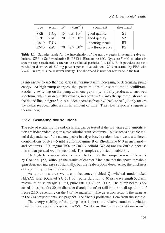
5.2 Experimental results
dye scatt. k n (cm−3) comment shorthand
SRB TiO2 15 1.8 ·1013 good quality STSRB ZnO 70 8.7 ·1014 good quality SZR640 TiO2 – – inhomogeneous RTR640 ZnO 70 8.7 ·1014 low fluorescence RZ
Table 5.1 Samples made for the investigation of the narrow peaks in scattering dye so-lutions. SRB is Sulforhodamine B, R640 is Rhodamine 640. Dyes are 5 mM solutions inspectroscopic methanol, scatterers are colloidal particles [44, 133]. Both powders are sus-pended in densities of 320 mg powder per ml dye solution. k is measured by EBS withλ = 632.8 nm, n is the scatterer density. The shorthand is used for reference in the text.
is insensitive to whether the series is measured with increasing or decreasing pumpenergy. At high pump energies, the spectrum does take some time to equilibrate.Suddenly switching on the pump at an energy of 8 µJ initially produces a narrowedspectrum, which subsequently relaxes, in about 2–3 s, into the spectrum shown asthe dotted line in figure 5.9. A sudden decrease from 8 µJ back to ≈ 3 µJ only makesthe peaks reappear after a similar amount of time. This slow response suggests athermal origin.
5.2.2 Scattering dye solutions
The role of scattering in random lasing can be tested if the scattering and amplifica-tion are independent, e.g. in a dye solution with scatterers. To also test a possible ma-terial dependence of the narrow peaks in a dye-based random laser, we test differentcombinations of dye—5 mM Sulforhodamine B or Rhodamine 640 in methanol—and scatterers—320 mg/ml TiO2 or ZnO-N colloid. We do not use ZnO-A becauseit is not suspended well in methanol. The samples are listed in table 5.1.
The high dye concentration is chosen to facilitate the comparison with the workby Cao et al. [53], although the results of chapter 3 indicate that the above-thresholdgain does not increase substantially, but the reabsorption does. Also, the thicknessof the amplifying layer decreases.
As a pump source we use a frequency-doubled Q-switched mode-lockedNd:YAG laser (Quantel YG-501 30), pulse duration < 40 ps, wavelength 532 nm,maximum pulse energy 0.7 mJ, pulse rate 10, 20 or 30 Hz. The pump beam is fo-cused to a spot of ≈ 20 µm diameter (barely out of, or still in, the small-spot limit offigure 2.10, depending on the of the material). The detection setup is the same asin the ZnO experiments, see page 99. The fiber is positioned 1 cm from the sample.
The energy stability of the pump laser is poor: the relative standard deviationfrom the mean pulse energy is 30–35%. We do use this laser as excitation source,
103
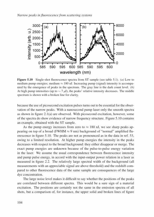
Narrow peaks in fluorescence from scattering systems
585 590 595 6000
500
1000
1500
2000
2500
3000 (a)
inte
nsity (
arb
. u.)
585 590 595 6000
2000
4000
6000
8000(b)
wavelength (nm)
Figure 5.10 Single-shot fluorescence spectra from ST sample (see table 5.1). (a) Low tomedium pump energies; medium ≈ 180 nJ. Increasing pump (signal) intensity is accompa-nied by the emergence of peaks in the spectrum. The gray line is the dark count level. (b)At high pump intensities (up to ∼ 7 µJ), the peaks’ relative intensity decreases. The middlespectrum is shown with a broken line for clarity.
because the use of picosecond excitation pulses turns out to be essential for the obser-vation of the narrow peaks. With a nanosecond pump laser only the smooth spectraas shown in figure 2.1(a) are observed. With picosecond excitation, however, someof the spectra do show evidence of narrow frequency structure. Figure 5.10 containsan example, obtained with the ST sample.
As the pump energy increases from zero to ≈ 180 nJ, we see sharp peaks ap-pearing on top of a broad (FWHM ≈ 9 nm) background of “normal” amplified flu-orescence in figure 5.10. The peaks are not as pronounced as in the data in ref. 53,owing to a limited resolution. At higher pump energies the intensity in the peaksdecreases with respect to the broad background: they either disappear or merge. Theexact pump energies are unknown because of the pulse-to-pulse energy variationin the laser. We assume the usual correspondence between fluorescence intensityand pump pulse energy, in accord with the input-output power relation in a laser asmeasured in figure 2.2. The relatively large spectral width of the background (allmeasurements with an appreciable signal are above threshold) and the redshift com-pared to other fluorescence data of the same sample are consequences of the largedye concentration.
The large noise level makes it difficult to say whether the positions of the peaksare correlated between different spectra. This would be a sure sign of a materialexcitation. The positions are certainly not the same in the emission spectra of allshots, but a comparison of, for instance, the upper solid and broken lines of figure
104
5.3 Discussion and conclusions
5.10(b), does suggest that the peak positions are not completely random.The spectra in figure 5.10 differ in the position of the center of the broad fluores-
cence band. It shifts randomly over a range of 2–3 nm. We did not observe this kindof shift with nanosecond excitation. The differences are possibly chemical in ori-gin, stemming from an interaction of the dye with the surface of the scatterers [135].Note that the TiO2 particles are surface treated with an (insulating) alumina/silicalayer. The scatterer surface is amorphous, hence many specific adsorption sites ex-ist. A small shot-to-shot variation at the onset of the emission-amplification processcould persist in the resulting measured spectrum due to the nonlinearity of the ASEprocess at high gain. Owing to the large intrinsic emission linewidth of the dye, sucha process does not seem a likely candidate as an explanation for the narrow peaks.
Repeating this experiment with the SZ sample—same dye, different scatterer,larger —yields qualitatively the same outcome. Compared to the ST measurements,the emission spectrum is redshifted by 6 nm, the recorded intensities are a factor 1.5–2 lower at the same pump intensity, and the number of peaks is smaller. The lowerintensity is a consequence of the higher threshold in this sample, caused by a larger. An interaction of the dye with the ZnO surface is readily apparent as the sample isprepared: upon addition of the scatterers the dye solution changes color from brightred/pink to deep purple. No change of color is observed if the coated TiO2 scatterersare used. This interaction of the dye with the scatterer surface could influence theemission spectrum.
The scatterers in the RT sample aggregate, and even after ultrasonic shakingthe suspension remains inhomogeneous. The RZ sample is identical to the materialused by Cao et al. [53]. We find that it luminesces weakly, and does not produce anyconvincing peaks at pump energies up to 50 µJ; above this energy the pump pulsedamages the glass of the sample container. We do not have an explanation for thediscrepancy between our measurements and those of ref. 53. The stability of thesuspension is markedly worse than the ST and SZ samples.
The pump pulse repetition rate profoundly influenced the ZnO emission. Avariation from 10 to 30 Hz is, however, found to have no effect on the appearance ofthe spikes in the dye-based ST and SZ samples.
5.3 Discussion and conclusions
In the previous section we have presented measurements, augmenting the data fromthe literature reviewed in section 5.1. Here we discuss how the additional experi-ments fit in or modify the picture sketched in earlier publications. We do not tryto answer the question whether or not the narrow peaks in ZnO are related to las-ing; in ref. 108 they were shown to be. The issue we address is the role of multiple
105
Narrow peaks in fluorescence from scattering systems
scattering in the laser process.First, we remark that all samples studied, by us and by others, are far from lo-
calization: the smallest values for k are achieved in the ZnO powder samples [131]and the dye samples with TiO2 scatterers, k ≈ 14. Considering that materials withk =3–4 still show predominantly diffusive behavior [26, 27], it is hasty to attributeany observation in less strongly scattering materials to localization. Even if the hand-wavingly substantiated hunch that gain facilitates localization (see page 91) turns outto be legitimate, the gap from k≥ 14 to the transition is huge, and observable effectsare at best improbable.
5.3.1 ZnO powders
The two ZnO powder samples react very differently to UV excitation, while theirk values are the same. ZnO-N only emits at high pump energy with an EHP-likespectrum. ZnO-A shows many narrow peaks in the exciton luminescence band.
In ZnO-A, we observed a surprisingly strong dependence of the emission spec-trum on the pump pulse repetition rate (figure 5.8) and an extreme nonlinearity as afunction of pump pulse energy (figure 5.9). Both phenomena are reversible, and bothrespond slowly, with a time constant of 2–3 s. The only likely candidate to producesuch a slow response is a thermal process. The absorbed pump energy is partly con-verted into heat, producing a local temperature increase. This effect should be morepronounced in a powder than in any other phase, on account of the poor thermalconductivity of an inhomogeneous structure.
Underlying process? What the elevated temperature might effectuate is a matterof speculation, which we will pursue only briefly. Narrow sub-gap peaks in photo-luminescence spectra have been observed in disordered or alloy II–VI semiconduc-tors [136], and even lasing has been reported [137]. The intensity in the peaks showsthe characteristic laser-like nonlinearity as a function of pump power. These nar-row spectral features have been attributed to complex states consisting of an excitonbound to a localized defect. The peaks are observed only up to a maximum tempera-ture, depending on the material, above which the exciton dissociates thermally fromthe defect and the emission disappears.
The stability of excitons in II–VI semiconductors under lasing conditions, how-ever, is disputed [138]. Exciton absorption is seen to bleach above the laser thresholdin quantum well lasers [139, 140]. Electron-hole recombination across the energygap, that is renomalized due to the Coulomb interaction, produces gain and lumi-nescence at the exciton energy, without an actual exciton population [141]. At roomtemperature, excitons are shown to be always unstable in these materials, owing
106
5.3 Discussion and conclusions
to the large coupling to other (continuum) states. On the other hand, the theory isdone for materials with a perfect crystal lattice, so defect-related excitations can notbe reproduced. Localized (bound) excitons have a much smaller coupling to otherstates, with dephasing times up to 4 orders of magnitude larger than extended (free)excitons [118].
Our experiments do not contain sufficient detail to decide whether the emissionwe see is excitonic or free carrier recombination across a renormalized energy gap,nor is this our prime interest. We do see a nonlinearity with a thermal-like timeresponse. Temperature-dependent excitations may seem peculiar in semiconductorsat room temperature, since most features are only observed at low temperatures. Twoenergy scales in ZnO are larger than the thermal energy kBT = 25 meV: the bulkexciton binding energy Eb = 60 meV, and the Urbach tailing parameter EU = 40meV [142], describing the exponential decay of the electronic density of states at theband edge due to defect states.
We propose that the pumping of the sample populates luminescent levels, andthat this process is facilitated by the heating of the powder by the pump absorption,enhancing the luminescence at high rep. rates, cf. figure 5.8. The narrow linewidthsobserved suggest a role for localized defect states. An increase of the pulse energy orrep. rate raises the temperature further, thermally dissociating the luminescent state,which we assume consists of one or more charge carriers bound to a lattice defect.Consequently, the emission vanishes.
Stimulated emission from a compound defect state is possible by the narrowlinewidth and concomitant large gain. ref. 108 shows the light to be coherent, soa resonant (amplitude) feedback mechanism is present. At these high gain levels,however, even a weak external reflection can be sufficient to provoke lasing.
An example of defect-exciton complex luminescence is donor-acceptor pair(DAP) emission. In this process an electron on a donor recombines with a holeon an acceptor nearby [109, 143]. The result is a regular series of peaks at fixedpositions due to the 1/r Coulomb energy term contributing to the emitted photonenergy, with r on the lattice. This regularity could not be established by an inventoryof literature data or our own. On the other hand, a signature of DAP emission is ablueshift with increasing pump energy, as clearly observed in figure 5.9.
Above, we have presented a speculative proposal for an origin of the narrow peaksin ZnO powders. The optics of highly excited semiconductors is a rich and complexfield of research [144], and especially the nature of the gain mechanism in II–VImaterials is a matter of debate, that we do not aspire to settle here. To summarize,we remark that we did not find evidence for a crucial role for multiple scatteringin the occurrence of the narrow peaks in ZnO powder luminescence, and that our
107
Narrow peaks in fluorescence from scattering systems
results suggest a thermally activated mechanism with a strongly nonlinear response.Which semiconductor electronic process produces these spectral features, and has acompatible temperature or intensity dependence, remains speculative. Similar peakshave been seen in homogeneous alloy semiconductors.
5.3.2 Dye suspensions
The results of the experiments on dyes with scatterers are not as conclusive, or sug-gestive, as those on ZnO, partially on account of the lesser data quality. Based on theobservations presented in section 5.2.2, the most straightforward conclusion is thatthe narrow peaks in this system are caused by scattering. The most strongly scat-tering (ST; cf. table 5.1) sample shows the strongest peaks, the scatterers in whichhappen to have a surface coating, reducing the interaction of the surface electronicstructure with the dye. We tried to test the influence of the material more stringentlyby increasing the scatterer concentration in the SZ sample but found that a denserZnO suspension is unstable and the colloid aggregates.
On closer inspection of the data in section 5.2.2, and comparing with the articleby Cao and coworkers [53], two issues arise:
The peaks are only observed with a picosecond excitation pulse, only the nor-mal narrowed spectrum appears with a nanosecond pump.
The RZ sample on which the published experiments by Cao et al. were per-formed showed no peaks in our experiments, and low luminescence. Eventhough its k is large, the absence of a convincing signal up to these highpump energies is surprising. On the other hand, the SZ sample does showpeaks, but has the same k (from EBS) as a sample where Cao et al. did notobserve any. The difference is the dye, the turbidity is the same.
The latter point only seems to indicate, if anything, a very sensitive dependenceof the narrow-peak appearance on material and preparation. The former is an ob-servation that needs to be explained if the phenomenon is to be given a theoreticalbacking in multiple scattering. If multiple scattering is to be responsible for the nar-row peaks, we must find a process causing the peaks, that happens on a time scale 50 ps, because the peaks do not average out with this excitation pulse length, but 500 ps, because there is no trace of the peaks with a nanosecond pump pulse.
In a nanosecond, a scattering medium is essentially static: particle motion in acolloidal suspension has a typical time scale of milliseconds. There are two pro-cesses in a diffusive random laser with time constants of the correct order. Thelongest detectable paths in a multiply scattering liquid medium dephase at a rate inthe GHz range; these dynamics are used in DWS. Constructive interference between
108
5.3 Discussion and conclusions
long paths is a particular speckle, which is not sufficiently wavelength specific. An-other process at a 10–100 ps time scale is the relaxation oscillation. This is notspectrally selective either.
Material-related processes with subnanosecond dynamics exist in great varietyin a system of dye on an oxide surface. It is not always clear whether these areaccompanied by narrow spectral features. Dye-like excitations have a large intrinsiclinewidth, maybe a combination with the surface electronic structure of the scatterercan give rise to narrow features. Our experiments are not sufficient to decide whethera particular type of excitations causes the sharp peaks.
5.3.3 Conclusions
We find a striking difference in luminescence properties of the two ZnO powders,differing in method of synthesis, particle size distribution, and surface properties,but not in purity or scattering characteristics. The light transport is undoubtedlydiffusive at k ≈ 14.
Furthermore, we measure a strong nonlinearity with a thermal-like time responsein the fluorescent emission of ZnO powders. These observations lead us to an in-terpretation of the narrow peaks in terms of material excitations, rather than onebased on the random laser concept. The explanation is compatible with, and evensupported by [109, 117] the data on these samples in the literature, and could be ap-plied to ZnO thin films. However, for the occurrence of narrow peaks in thin filmsthere is another, more elegant candidate, that is supported by direct experimentalevidence [126]: the formation of Fabry-Perot cavities by grain boundaries betweenpumped and unpumped material, proposed in section 5.1.3. The only data that lacka consistent interpretation are those on scattering dye suspensions. Our findings par-tially contradict the results in the literature.
Superfluous as it may seem, there could be three different mechanisms at work,producing very similar-looking narrow peaks in different materials. One can alsoresort to the semi-skeptical statement that it must be some electronic excitation inall cases, the nature of which can be speculated on in ZnO, and is left unspecified inthe dye materials. We opt for two processes: the cavities in the transparent films andan electronic excitation in the multiply scattering materials. The latter explanation isadopted for the dye suspensions only because the alternatives must be discarded; forthe ZnO powders it is quite firmly supported by experimental data.
109

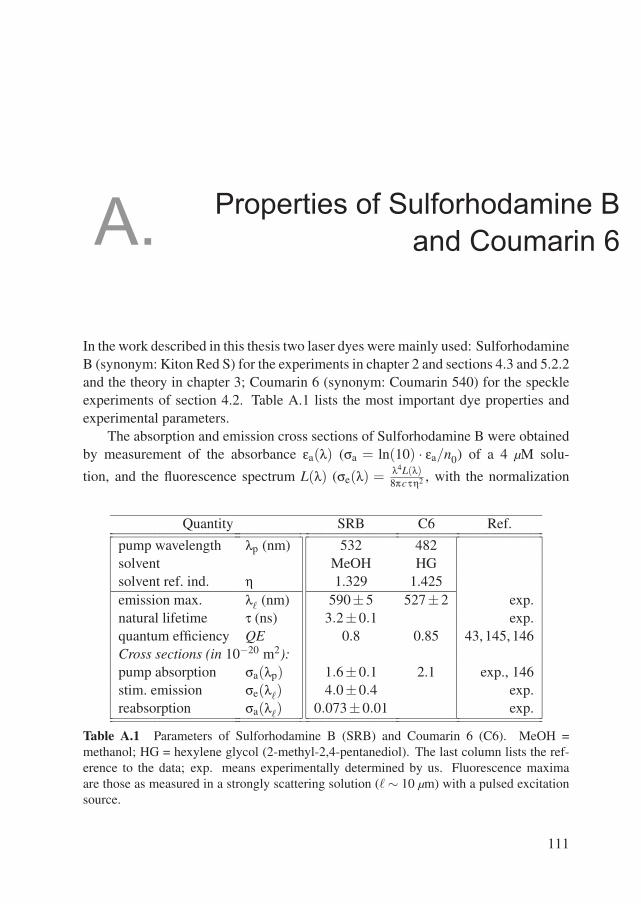
A.Properties of Sulforhodamine B
and Coumarin 6
In the work described in this thesis two laser dyes were mainly used: SulforhodamineB (synonym: Kiton Red S) for the experiments in chapter 2 and sections 4.3 and 5.2.2and the theory in chapter 3; Coumarin 6 (synonym: Coumarin 540) for the speckleexperiments of section 4.2. Table A.1 lists the most important dye properties andexperimental parameters.
The absorption and emission cross sections of Sulforhodamine B were obtainedby measurement of the absorbance εa(λ) (σa = ln(10) · εa/n0) of a 4 µM solu-
tion, and the fluorescence spectrum L(λ) (σe(λ) = λ4L(λ)8πcτη2 , with the normalization
Quantity SRB C6 Ref.
pump wavelength λp (nm) 532 482solvent MeOH HGsolvent ref. ind. η 1.329 1.425emission max. λ (nm) 590±5 527±2 exp.natural lifetime τ (ns) 3.2±0.1 exp.quantum efficiency QE 0.8 0.85 43, 145, 146Cross sections (in 10−20 m2):pump absorption σa(λp) 1.6±0.1 2.1 exp., 146stim. emission σe(λ) 4.0±0.4 exp.reabsorption σa(λ) 0.073±0.01 exp.
Table A.1 Parameters of Sulforhodamine B (SRB) and Coumarin 6 (C6). MeOH =methanol; HG = hexylene glycol (2-methyl-2,4-pentanediol). The last column lists the ref-erence to the data; exp. means experimentally determined by us. Fluorescence maximaare those as measured in a strongly scattering solution ( ∼ 10 µm) with a pulsed excitationsource.
111
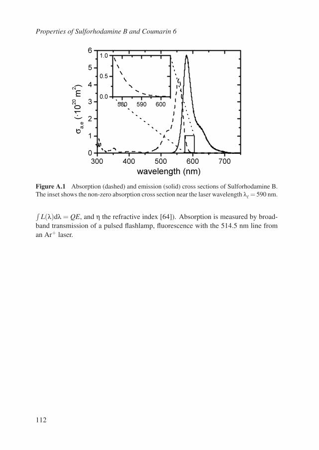
Properties of Sulforhodamine B and Coumarin 6
300 400 500 600 700
0
1
2
3
4
5
6
σ a,e (
·1020 m
2)
wavelength (nm)
580 590 600
0.0
0.5
1.0
Figure A.1 Absorption (dashed) and emission (solid) cross sections of Sulforhodamine B.The inset shows the non-zero absorption cross section near the laser wavelength λ = 590 nm.
∫L(λ)dλ = QE, and η the refractive index [64]). Absorption is measured by broad-
band transmission of a pulsed flashlamp, fluorescence with the 514.5 nm line froman Ar+ laser.
112
B.Pump units and terminology
In experiments related to the laser threshold, it is important to correctly quantifythe pump energy supply. The most basic mechanism involved in introducing andmaintaining gain in the laser is the transfer of population from the ground state tothe excited state. Laser rate equations usually incorporate a term that describes thisprocess as the pump rate: number of dye molecules excited per second. The numberof excited dye molecules is proportional to the amount of supplied energy and to N0,the number of available molecules in the ground state. Power (P), the rate of energysupply, is the crucial quantity.
We use optical pumping, so the energy is supplied by photons. The number ofexcited molecules is equal to the number of absorbed photons, and probability of anincident photon being absorbed is given by the absorption cross section, which is anarea, relative to the total area A of the exciting beam. Apparently, we have to considerthe flux density F of photons, number per unit time per unit area. Then the pumprate becomes r = F ·N0 ·σa. F is related to the intensity I by I = F ·hωp = P/A. Forhomogeneous optical pumping, the intensity (in W ·m−2) is the most straightforwardquantity to use.
In an inhomogeneous system like ours there is a catch: we have to consider theenergy supply to a small volume around each point because quantities vary locally.This is most easily done by working in terms of volume densities, i.e. number of dyemolecules and amount of pump energy per unit volume. Writing the pump energydensity as Wp = I ·c/hωp, we arrive at a pump rate density Rd =Wp ·c ·σa ·n0, where cis the propagation speed of light in the medium and n0 is the density of dye moleculesin the ground state. Rd is the number of dye molecules per unit volume excited perunit time (m−3s−1).
This pump rate density depends on the pump light density, resulting from theincident beam, which is measured in our pulsed experiments in units of fluence,
113
Pump units and terminology
J ·m−2. The connection between these two quantities, flux density in a plane waveand light density in a diffusing field is a well-studied problem, see ref. 15. Incidentlight is usually introduced by placing a diffuse source at a distance of one mean freepath from the surface, or like in our calculations, by using an exponentially decayingsource intensity [147]. The source has to be properly normalized to make quantita-tive comparison with experiments possible. The local and instantaneous light densityis a solution of the diffusion equation, see chapter 3.
114
R.References
[1] M. Born and E. Wolf, Principles of Optics, 6th ed., Pergamon, Oxford (1980), sect.2.3.4.
[2] J. D. Jackson, Classical Electrodynamics, 2nd ed., John Wiley & Sons, New York(1975), sect. 4.3–5, and 6.7.
[3] R. Loudon, The Quantum Theory of Light, 2nd ed., Oxford University Press, Oxford(1983), sect. 8.2, 8.6 and 8.7.
[4] D. P. Craig and T. Thirunamachandran, Molecular Quantum Electrodynamics, Aca-demic Press, London (1984), p. 131.
[5] J. D. Jackson, op. cit. [2], pp. 418–422.[6] A. Lagendijk and B. A. van Tiggelen, Resonant multiple scattering of light, Phys.
Rep. 270, 143–216, sect. 2.[7] C. F. Bohren and D. R. Huffman, Absorption and Scattering of Light by Small Parti-
cles, John Wiley & Sons, New York (1983), pp. 130–132.[8] Lord Rayleigh, On the Light from the Sky, its Polarization and Colour, Philos. Mag.
41, 107–120, 274–279 (quoted in ref. 7); On the Scattering of Light by Small Parti-cles, ibid., pp. 447–454.
[9] H. C. van de Hulst, Light Scattering by Small Particles, Dover Publishing, New York(1981), p. 114.
[10] R. P. Feynman, R. B. Leighton, and M. Sands, The Feynman Lectures on Physics,Addison-Wesley, Reading (1963), vol. 1, sect. 32-5.
[11] C. F. Bohren and D. R. Huffman, op. cit. [7], chapter 4. The book also gives a Fortranprogram to calculate scattering and absorption cross sections, scattering angles, etc.
[12] H. C. van de Hulst, op. cit. [9], sect. 13.2.[13] V. Sandoghar, F. Treussart, J. Hare, V. Lefevre-Seguin, J. M. Raimond, and S.
Haroche, Very low threshold whispering-gallery-mode microsphere laser, Phys. Rev.A 54, R1777–R1780 (1996).
[14] M. Born and E. Wolf, op. cit. [1], sect. 13.1 and 13.2.[15] A. Ishimaru, Wave Propagation and Scattering in Random Media, Academic Press,
New York, 1978, pp. 175–183.[16] B. A. van Tiggelen and A. Lagendijk, Analogies between light and electrons? and
Coherent beam, diffuse beam and speckles: the old view, sect. 1.1 and 1.2, in: POANResearch Group (Ed.), New Aspects of Electromagnetic and Acoustic Wave Diffusion,Springer Tracts in Modern Physics, vol. 144, Springer, Berlin (1998).
[17] M. P. van Albada, B. A. van Tiggelen, A. Lagendijk, and A. Tip, Speed of propaga-
115
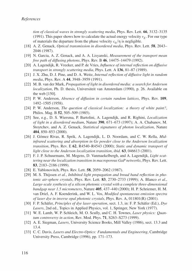
References
tion of classical waves in strongly scattering media, Phys. Rev. Lett. 66, 3132–3135(1991). This paper shows how to calculate the actual energy velocity vE . For our typeof materials the departure from the phase velocity c0/η is negligible.
[18] A. Z. Genack, Optical transmission in disordered media, Phys. Rev. Lett. 58, 2043–2046 (1987).
[19] N. Garcia, A. Z. Genack, and A. A. Lisyanski, Measurement of the transport meanfree path of diffusing photons, Phys. Rev. B 46, 14475–14479 (1992).
[20] A. Lagendijk, R. Vreeker, and P. de Vries, Influence of internal reflection on diffusivetransport in strongly scattering media, Phys. Lett. A 136, 81–87 (1989).
[21] J. X. Zhu, D. J. Pine, and D. A. Weitz, Internal reflection of diffusive light in randommedia, Phys. Rev. A 44, 3948–3959 (1991).
[22] M. B. van der Mark, Propagation of light in disordered media: a search for Andersonlocalization, Ph. D. thesis, Universiteit van Amsterdam (1990), p. 26. Available onthe web [150].
[23] P. W. Anderson, Absence of diffusion in certain random lattices, Phys. Rev. 109,1492–1505 (1958).
[24] P. W. Anderson, The question of classical localization: a theory of white paint?,Philos. Mag. B 52, 505–509 (1985).
[25] See, e.g., D. S. Wiersma, P. Bartolini, A. Lagendijk, and R. Righini, Localizationof light in a disordered medium, Nature 390, 671–673 (1997); A. A. Chabanov, M.Stoytchev, and A. Z. Genack, Statistical signatures of photon localization, Nature404, 850–853 (2000).
[26] J. Gomez Rivas, R. Sprik, A. Lagendijk, L. D. Noordam, and C. W. Rella, Mid-infrared scattering and absorption in Ge powder close to the Anderson localizationtransition, Phys. Rev. E 62, R4540–R4543 (2000); Static and dynamic transport oflight close to the Anderson localization transition, ibid. 63, 046613 (2001).
[27] F. J. P. Schuurmans, M. Megens, D. Vanmaekelbergh, and A. Lagendijk, Light scat-tering near the localization transition in macroporous GaP networks, Phys. Rev. Lett.83, 2183–2186 (1999).
[28] E. Yablonovitch, Phys. Rev. Lett. 58, 2059–2062 (1987).[29] M. S. Thijssen et al., Inhibited light propagation and broad band reflection in pho-
tonic air-sphere crystals, Phys. Rev. Lett. 83, 2730–2733 (1999); A. Blanco et al.,Large-scale synthesis of a silicon photonic crystal with a complete three-dimensionalbandgap near 1.5 micrometers, Nature 405, 437–440 (2000); H. P. Schriemer, H. M.van Driel, A. F. Koenderink, and W. L. Vos, Modified spontaneous emission spectraof laser dye in inverse opal photonic crystals, Phys. Rev. A, 011801(R) (2001).
[30] F. P. Schafer, Principles of dye laser operation, sect. 1.3, in: F. P. Schafer (Ed.), DyeLasers, 2nd ed., Topics in Applied Physics, vol. 1, Springer, New York (1977).
[31] W. E. Lamb, W. P. Schleich, M. O. Scully, and C. H. Townes, Laser physics: Quan-tum controversy in action, Rev. Mod. Phys. 71, S263–S273 (1999).
[32] A. E. Siegman, Lasers, University Science Books, Mill Valley (1986), sect. 13.3 and13.4.
[33] C. C. Davis, Lasers and Electro-Optics: Fundamentals and Engineering, CambridgeUniversity Press, Cambridge (1996), pp. 171–173.
116
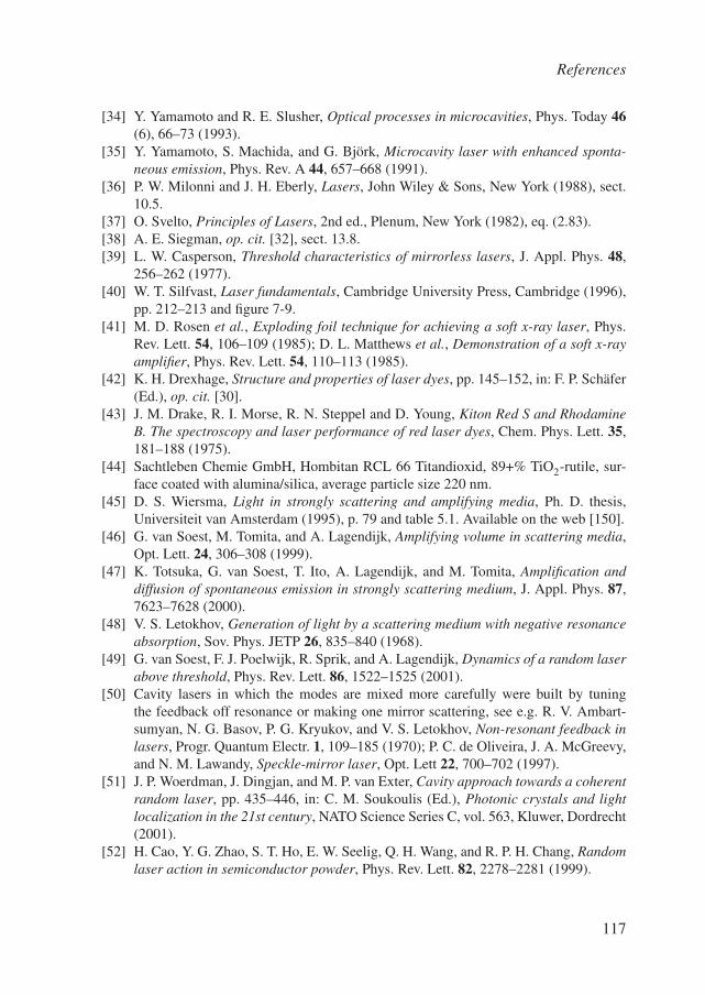
References
[34] Y. Yamamoto and R. E. Slusher, Optical processes in microcavities, Phys. Today 46(6), 66–73 (1993).
[35] Y. Yamamoto, S. Machida, and G. Bjork, Microcavity laser with enhanced sponta-neous emission, Phys. Rev. A 44, 657–668 (1991).
[36] P. W. Milonni and J. H. Eberly, Lasers, John Wiley & Sons, New York (1988), sect.10.5.
[37] O. Svelto, Principles of Lasers, 2nd ed., Plenum, New York (1982), eq. (2.83).[38] A. E. Siegman, op. cit. [32], sect. 13.8.[39] L. W. Casperson, Threshold characteristics of mirrorless lasers, J. Appl. Phys. 48,
256–262 (1977).[40] W. T. Silfvast, Laser fundamentals, Cambridge University Press, Cambridge (1996),
pp. 212–213 and figure 7-9.[41] M. D. Rosen et al., Exploding foil technique for achieving a soft x-ray laser, Phys.
Rev. Lett. 54, 106–109 (1985); D. L. Matthews et al., Demonstration of a soft x-rayamplifier, Phys. Rev. Lett. 54, 110–113 (1985).
[42] K. H. Drexhage, Structure and properties of laser dyes, pp. 145–152, in: F. P. Schafer(Ed.), op. cit. [30].
[43] J. M. Drake, R. I. Morse, R. N. Steppel and D. Young, Kiton Red S and RhodamineB. The spectroscopy and laser performance of red laser dyes, Chem. Phys. Lett. 35,181–188 (1975).
[44] Sachtleben Chemie GmbH, Hombitan RCL 66 Titandioxid, 89+% TiO2-rutile, sur-face coated with alumina/silica, average particle size 220 nm.
[45] D. S. Wiersma, Light in strongly scattering and amplifying media, Ph. D. thesis,Universiteit van Amsterdam (1995), p. 79 and table 5.1. Available on the web [150].
[46] G. van Soest, M. Tomita, and A. Lagendijk, Amplifying volume in scattering media,Opt. Lett. 24, 306–308 (1999).
[47] K. Totsuka, G. van Soest, T. Ito, A. Lagendijk, and M. Tomita, Amplification anddiffusion of spontaneous emission in strongly scattering medium, J. Appl. Phys. 87,7623–7628 (2000).
[48] V. S. Letokhov, Generation of light by a scattering medium with negative resonanceabsorption, Sov. Phys. JETP 26, 835–840 (1968).
[49] G. van Soest, F. J. Poelwijk, R. Sprik, and A. Lagendijk, Dynamics of a random laserabove threshold, Phys. Rev. Lett. 86, 1522–1525 (2001).
[50] Cavity lasers in which the modes are mixed more carefully were built by tuningthe feedback off resonance or making one mirror scattering, see e.g. R. V. Ambart-sumyan, N. G. Basov, P. G. Kryukov, and V. S. Letokhov, Non-resonant feedback inlasers, Progr. Quantum Electr. 1, 109–185 (1970); P. C. de Oliveira, J. A. McGreevy,and N. M. Lawandy, Speckle-mirror laser, Opt. Lett 22, 700–702 (1997).
[51] J. P. Woerdman, J. Dingjan, and M. P. van Exter, Cavity approach towards a coherentrandom laser, pp. 435–446, in: C. M. Soukoulis (Ed.), Photonic crystals and lightlocalization in the 21st century, NATO Science Series C, vol. 563, Kluwer, Dordrecht(2001).
[52] H. Cao, Y. G. Zhao, S. T. Ho, E. W. Seelig, Q. H. Wang, and R. P. H. Chang, Randomlaser action in semiconductor powder, Phys. Rev. Lett. 82, 2278–2281 (1999).
117
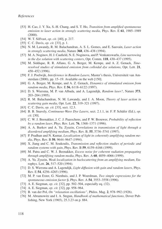
References
[53] H. Cao, J. Y. Xu, S.-H. Chang, and S. T. Ho, Transition from amplified spontaneousemission to laser action in strongly scattering media, Phys. Rev. E 61, 1985–1989(2000).
[54] W. T. Silfvast, op. cit. [40], p. 217.[55] C. C. Davis, op. cit. [33], p. 1.[56] N. M. Lawandy, R. M. Balachandran, A. S. L. Gomes, and E. Sauvain, Laser action
in strongly scattering media, Nature 368, 436–438 (1994).[57] M. A. Noginov, H. J. Caufield, N. E. Noginova, and P. Venkateswarlu, Line narrowing
in the dye solution with scattering centers, Opt. Comm. 118, 430–437 (1995).[58] M. Siddique, R. R. Alfano, G. A. Berger, M. Kempe, and A. Z. Genack, Time-
resolved studies of stimulated emission from colloidal dye solutions, Opt. Lett. 21,450–452 (1996).
[59] F. J. Poelwijk, Interference in Random Lasers, Master’s thesis, Universiteit van Am-sterdam (2000), pp. 15–19. Available on the web [150].
[60] G. A. Berger, M. Kempe, and A. Z. Genack, Dynamics of stimulated emisson fromrandom media, Phys. Rev. E 56, 6118–6122 (1997).
[61] D. S. Wiersma, M. P. van Albada, and A. Lagendijk, Random laser?, Nature 373,203–204 (1995).
[62] R. M. Balachandran, N. M. Lawandy, and J. A. Moon, Theory of laser action inscattering gain media, Opt. Lett. 22, 319–321 (1997).
[63] C. C. Davis, op. cit. [33], sect. 12.3.[64] B. B. Snavely, Continuous-Wave Dye Lasers, sect. 2.1.1, in: F. P. Schafer (Ed.), op.
cit. [30].[65] C. W. J. Beenakker, J. C. J. Paasschens, and P. W. Brouwer, Probability of reflection
by a random laser, Phys. Rev. Lett. 76, 1368–1371 (1996).[66] A. A. Burkov and A. Yu. Zyuzin, Correlations in transmission of light through a
disordered amplifying medium, Phys. Rev. B, 55, 5736–5741 (1997).[67] P. Pradhan and N. Kumar, Localization of light in coherently amplifying random me-
dia, Phys. Rev. B 50, 9644–9647 (1994).[68] X. Jiang and C. M. Soukoulis, Transmission and reflection studies of periodic and
random systems with gain, Phys. Rev. B 59, 6159–6166 (1999).[69] M. Patra and C. W. J. Beenakker, Excess noise for coherent radiation propagating
through amplifying random media, Phys. Rev. A 60, 4059–4066 (1999).[70] A. Yu. Zyuzin, Weak localization in backscattering from an amplifying medium, Eu-
rophys. Lett. 26, 517–520 (1994).[71] D. S. Wiersma and A. Lagendijk, Light diffusion with gain and random lasers, Phys.
Rev. E 54, 4256–4265 (1996).[72] M. P. van Exter, G. Nienhuis, and J. P. Woerdman, Two simple expressions for the
spontaneous emission factor β, Phys. Rev. A 54, 3553–3558 (1996).[73] A. E. Siegman, op. cit. [32], pp. 502–504, especially eq. (32).[74] A. E. Siegman, op. cit. [32], pp. 958–964.[75] B. van der Pol, On “relaxation oscillations”, Philos. Mag. 2, 978–992 (1926).[76] M. Abramowitz and I. A. Stegun, Handbook of mathematical functions, Dover Pub-
lishing, New York (1965), 25.3.23 on p. 884.
118
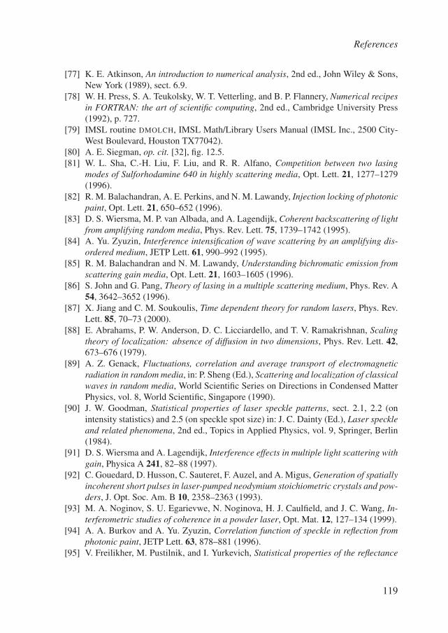
References
[77] K. E. Atkinson, An introduction to numerical analysis, 2nd ed., John Wiley & Sons,New York (1989), sect. 6.9.
[78] W. H. Press, S. A. Teukolsky, W. T. Vetterling, and B. P. Flannery, Numerical recipesin FORTRAN: the art of scientific computing, 2nd ed., Cambridge University Press(1992), p. 727.
[79] IMSL routine DMOLCH, IMSL Math/Library Users Manual (IMSL Inc., 2500 City-West Boulevard, Houston TX77042).
[80] A. E. Siegman, op. cit. [32], fig. 12.5.[81] W. L. Sha, C.-H. Liu, F. Liu, and R. R. Alfano, Competition between two lasing
modes of Sulforhodamine 640 in highly scattering media, Opt. Lett. 21, 1277–1279(1996).
[82] R. M. Balachandran, A. E. Perkins, and N. M. Lawandy, Injection locking of photonicpaint, Opt. Lett. 21, 650–652 (1996).
[83] D. S. Wiersma, M. P. van Albada, and A. Lagendijk, Coherent backscattering of lightfrom amplifying random media, Phys. Rev. Lett. 75, 1739–1742 (1995).
[84] A. Yu. Zyuzin, Interference intensification of wave scattering by an amplifying dis-ordered medium, JETP Lett. 61, 990–992 (1995).
[85] R. M. Balachandran and N. M. Lawandy, Understanding bichromatic emission fromscattering gain media, Opt. Lett. 21, 1603–1605 (1996).
[86] S. John and G. Pang, Theory of lasing in a multiple scattering medium, Phys. Rev. A54, 3642–3652 (1996).
[87] X. Jiang and C. M. Soukoulis, Time dependent theory for random lasers, Phys. Rev.Lett. 85, 70–73 (2000).
[88] E. Abrahams, P. W. Anderson, D. C. Licciardello, and T. V. Ramakrishnan, Scalingtheory of localization: absence of diffusion in two dimensions, Phys. Rev. Lett. 42,673–676 (1979).
[89] A. Z. Genack, Fluctuations, correlation and average transport of electromagneticradiation in random media, in: P. Sheng (Ed.), Scattering and localization of classicalwaves in random media, World Scientific Series on Directions in Condensed MatterPhysics, vol. 8, World Scientific, Singapore (1990).
[90] J. W. Goodman, Statistical properties of laser speckle patterns, sect. 2.1, 2.2 (onintensity statistics) and 2.5 (on speckle spot size) in: J. C. Dainty (Ed.), Laser speckleand related phenomena, 2nd ed., Topics in Applied Physics, vol. 9, Springer, Berlin(1984).
[91] D. S. Wiersma and A. Lagendijk, Interference effects in multiple light scattering withgain, Physica A 241, 82–88 (1997).
[92] C. Gouedard, D. Husson, C. Sauteret, F. Auzel, and A. Migus, Generation of spatiallyincoherent short pulses in laser-pumped neodymium stoichiometric crystals and pow-ders, J. Opt. Soc. Am. B 10, 2358–2363 (1993).
[93] M. A. Noginov, S. U. Egarievwe, N. Noginova, H. J. Caulfield, and J. C. Wang, In-terferometric studies of coherence in a powder laser, Opt. Mat. 12, 127–134 (1999).
[94] A. A. Burkov and A. Yu. Zyuzin, Correlation function of speckle in reflection fromphotonic paint, JETP Lett. 63, 878–881 (1996).
[95] V. Freilikher, M. Pustilnik, and I. Yurkevich, Statistical properties of the reflectance
119
References
and transmittance of an amplifying random medium, Phys. Rev. B 56, 5974–5977(1997).
[96] A. Yu. Zyuzin, Transmission fluctuations and spectral rigidity of lasing states in arandom amplifying medium, Phys. Rev. E 51, 5274–5278 (1995).
[97] G. Parry, Speckle patterns in partially coherent light, sect. 3.1 and 3.2 in: J. C. Dainty(Ed.), op. cit. [90].
[98] J. F. de Boer, Optical fluctuations on the transmission and reflection of mesoscopicsystems, Ph.D. thesis, Universiteit van Amsterdam (1995), sect. 3.3.2 and 3.4.2.Available on the web [150].
[99] K. M. Watson, Multiple scattering of electromagnetic waves in an underdenseplasma, J. Math. Phys. 10, 688–702 (1969); Y. Kuga and A. Ishimaru, Retroreflec-tion from a dense distribution of spherical particles, J. Opt. Soc. Am. A 8, 831–835(1984); M. P. van Albada and A. Lagendijk, Observation of weak localization oflight in a random medium, Phys. Rev. Lett. 55, 2692–2695 (1985); P. E. Wolf andG. Maret, Weak localization and coherent backscattering of photons in disorderedmedia, Phys. Rev. Lett. 55, 2696–2699 (1985).
[100] P. C. de Oliveira, A. E. Perkins, and N. M. Lawandy, Coherent backscattering fromhigh-gain scattering media, Opt. Lett. 21, 1685–1687 (1996).
[101] W. Deng, D. S. Wiersma, and Z. Q. Zhang, Coherent backscattering of light from ran-dom media with inhomogeneous gain coefficient, Phys. Rev. B 56, 178–181 (1997).
[102] A. Z. Genack and J. M. Drake, Scattering for super-radiation, Nature 368, 400–401(1994).
[103] D. J. Pine, D. A. Weitz, P. M. Chaikin, and E. Herbolzheimer, Diffusing wave spec-troscopy, Phys. Rev. Lett. 60, 1134–1137 (1988).
[104] M. B. van der Mark, op. cit. [22], pp. 56–57.[105] H. Cao et al., Ultraviolet lasing in resonators formed by scattering in semiconductor
polycrystalline films, Appl. Phys. Lett. 73, 3656–3658 (1998).[106] H. Cao, J. Y. Xu, E. W. Seelig, and R. P. H. Chang, Microlaser made of disordered
media, Appl. Phys. Lett. 76, 2997–2999 (2000).[107] H. Cao et al., Spatial confinement of light in active random media, Phys. Rev. Lett.
84, 5584–5587 (2000).[108] H. Cao, Y. Ling, J. Y. Xu, C. Q. Cao, and P. Kumar, Photon statistics of random
lasers with resonant feedback, Phys. Rev. Lett. 86, 4524–4527 (2001).[109] Y. Sun, J. B. Ketterson, and G. K. L. Wong, Excitonic gain and stimulated ultravio-
let emission in nanocrystalline zinc-oxide powder, Appl. Phys. Lett. 77, 2322–2324(2000).
[110] A. Mitra and R. K. Thareja, Photoluminescence and ultraviolet laser emission fromnanocrystalline ZnO thin films, J. Appl. Phys. 89, 2025–2028 (2001).
[111] H. Cao, Y. G. Zhao, H. C. Ong, and R. P. H. Chang, Far-field characteristics ofrandom lasers, Phys. Rev. B 59, 15107–15111 (1999).
[112] H. Cao, Y. G. Zhao, X. Liu, E. W. Seelig, and R. P. H. Chang, Effect of externalfeedback on lasing in random media, Appl. Phys. Lett. 75, 1213–1215 (1999).
[113] S. Cho, J. Ma, Y. Kim, Y. Sun, G. K. L. Wong, and J. B. Ketterson, Photolumi-nescence and ultraviolet lasing of polycrystalline ZnO thin films prepared by the
120
References
oxidation of the metallic Zn, Appl. Phys. Lett. 75, 2761–2763 (1999).[114] S. V. Frolov, Z. V. Vardeny, K. Yoshino, A. Zakhidov, and R. Baughman, Stimulated
emission in high-gain organic media, Phys. Rev. B 59, R5284–R5287 (1999).[115] M. N. Shkunov, M. C. DeLong, M. E. Raikh, Z. V. Vardeny, A. A. Zakhidov, and
R. H. Baughman, Photonic versus random lasing in opal photonic single crystals,Synth. Met. 116, 485–491 (2001).
[116] D. S. Wiersma, M. P. van Albada, and A. Lagendijk, Experimental evidence for recur-rent multiple scattering of light in disordered media, Phys. Rev. Lett. 74, 4193–4196(1995).
[117] H. J. Egelhaaf and D. Oelkrug, Luminescence and nonradiative deactivation of ex-cited states involving oxygen defect centers in polycrystalline ZnO, J. Cryst. Growth161, 190–194 (1996).
[118] C. F. Klingshirn, Linear and nonlinear optics of wide-gap II-VI semiconductors,Phys. Stat. Sol. B 202, 857–871 (1997).
[119] C. F. Klingshirn, Semiconductor optics, Springer, Berlin (1997), ch. 15 and 21.[120] J. Gomez Rivas, R. Sprik, and A. Lagendijk, Optical transmission through very
strong scattering media, Ann. Phys. (Leipzig) 8, Spec. Issue, 77–80 (1999).[121] For a review, see: P. V. Kamat, Photochemistry on nonreactive and reactive (semi-
conductor) surfaces, Chem. Rev. 93, 267–300 (1993).[122] M. Kaveh, Localization of photons in disordered systems, Philos. Mag. B 56, 693–
703 (1987).[123] M. A. Lax, Multiple scattering of waves, Rev. Mod. Phys. 23, 287–310 (1951).[124] E. N. Economou and C. M. Soukoulis, Connection of localization with the problem
of the bound state in a potential well, Phys. Rev. B 28, 1093–1094 (1983); E. N.Economou, C. M. Soukoulis, and A. D. Zdetsis, Localized states in disordered sys-tems as bound states in potential wells, Phys. Rev. B 30, 1686–1694 (1984).
[125] R. Lang and K. Kobayashi, External optical feedback effects on semiconductor injec-tion laser properties, IEEE J. Quantum El. 16, 347–355 (1980).
[126] Z. K. Tang et al., Room-temperature ultraviolet laser emission from self-assembledZnO microcrystallite thin films, Appl. Phys. Lett. 72, 3270–3273 (1998); M.Kawasaki et al., Excitonic ultraviolet laser emission at room temperature from natu-rally made cavity in ZnO nanocrystal thin films, Mat. Sci. Eng. B 56, 239–245 (1998).
[127] P. L. Washington, H. C. Ong, J. Y. Dai, and R. P. H. Chang, Determination of theoptical constants of zinc oxide thin films by spectroscopic ellipsometry, Appl. Phys.Lett. 72, 3261–3263 (1998).
[128] M. J. Weber (Ed.), CRC Handbook of laser science and technology, vol. III. Opticalmaterials: part 1, CRC Press, Boca Raton, Florida (1986), table 1.1.17.128, p. 197.
[129] H. M. van Driel, Kinetics of high-density plasmas generated in Si by 1.06- and 0.53-µm picosecond laser pulses, Phys. Rev. B 35, 8166–8176 (1987); L. Huang, J. P.Callan, E. N. Glezer, and E. Mazur, GaAs under ultrafast excitation: response of thedielectric function, Phys. Rev. Lett. 80, 185–188 (1998).
[130] D. S. Wiersma, M. P. van Albada, and A. Lagendijk, An accurate technique to recordthe angular distribution of backscattered light, Rev. Sci. Instrum. 66, 5473–5476(1995).
121
References
[131] H. Cao et al., Random lasers with coherent feedback, p. 393 and fig. 4, in: C. M.Soukoulis (Ed.), op. cit. [51].
[132] Aldrich Zinc Oxide, powder, < 1 µm, 99.9% ZnO. On SEM photos most particles areseen to be rod-like, with aspect ratios ≈ 2, and sizes < 100 nm.
[133] Nanophase NanoTek©R 1701 Zinc Oxide, 99+% ZnO, average particle size: 24–71 nm;morphology: elongated; crystal phase: zincite (hexagonal).
[134] D. S. Wiersma, op. cit. [45], table 3.1.[135] K. Kemnitz, N. Tamai, I. Yamazaki, N. Nakashima, and K. Yoshihara, Fluorescence
decays and spectral properties of Rhodamine B in submono-, mono-, and multilayersystems, J. Phys. Chem. 90, 5094–5101 (1986).
[136] E. Cohen and M. D. Sturge, Fluorescence line narrowing, localized exciton states,and spectral diffusion in the mixed semiconductor CdSxSe1−x, Phys. Rev. B 25, 3828–3840 (1982).
[137] F. A. Majumder, S. Shevel, V. G. Lyssenko, H. E. Swoboda, and C. Klingshirn, Lu-minescence and gain spectroscopy of disordered CdS1−xSex under high excitation, Z.Phys. B 66, 409–418 (1987).
[138] S. Hughes, A. Knorr, S. W. Koch, R. Binder, R. Indik, and J. V. Moloney, The influ-ence of electron-hole scattering on the gain spectra of highly excited semiconductors,Solid State Comm. 100, 555–559 (1996); I. Galbraith and S. W. Koch, A comparisonof lasing mechanisms in ZnSe and GaAs, J. Cryst. Growth 159, 667–671 (1996); M.F. Pereira, Jr. and K. Henneberger, Gain mechanisms and lasing in II–VI compounds,Phys. Stat. Sol. B 202, 751–762 (1997).
[139] A. Diessel et al., Bleaching of excitonic absorption in II–VI laser diodes under lasingconditions, J. Cryst. Growth 159, 661–666 (1996).
[140] A. Yamamoto, T. Kido, T. Goto, Y. Chen, T. Yao, and A. Kasuya, Dynamics of pho-toexcited carriers in ZnO epitaxial thin films, Appl. Phys. Lett. 75, 469–471 (1999).
[141] M. Kira, F. Jahnke, and S. W. Koch, Microscopic theory of excitonic signaturesin semiconductor photoluminescence, Phys. Rev. Lett. 81, 3263–3266 (1998); A.Girndt, S. W. Koch, and W. W. Chow, Microscopic theory of laser gain in semicon-ductor quantum wells, Appl. Phys. A 66, 1–12 (1998).
[142] H. C. Ong, A. S. K. Li, and G. T. Du, Depth profiling of ZnO thin films by cathodo-luminescence, Appl. Phys. Lett. 78, 2667–2669 (2001).
[143] P. Y. Yu and M. Cardona, Fundamentals of semiconductors: physics and materialsproperties, Springer, Berlin (1996), pp. 344–349.
[144] C. Klingshirn and H. Haug, Optical properties of highly excited direct gap semicon-ductors, Phys. Rep. 70, 315–398 (1981).
[145] Kodak Laser Dyes, Eastman Kodak Company, Rochester (1987).[146] U. Brackmann, Lambdachrome Laser Dyes, Lambda Physik GmbH, Gottingen, Ger-
many (1995).[147] A. Ishimaru, op. cit. [15], eq. (8-6).[148] R. Loudon, op. cit. [3], p. 17.[149] P. W. Milonni and J. H. Eberly, op. cit. [36], p. 223.[150] http://www.science.uva.nl/research/scm/#theses
122
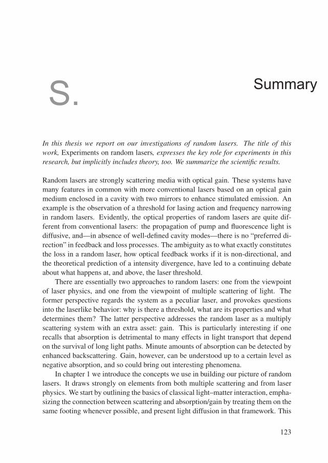
S.Summary
In this thesis we report on our investigations of random lasers. The title of thiswork, Experiments on random lasers, expresses the key role for experiments in thisresearch, but implicitly includes theory, too. We summarize the scientific results.
Random lasers are strongly scattering media with optical gain. These systems havemany features in common with more conventional lasers based on an optical gainmedium enclosed in a cavity with two mirrors to enhance stimulated emission. Anexample is the observation of a threshold for lasing action and frequency narrowingin random lasers. Evidently, the optical properties of random lasers are quite dif-ferent from conventional lasers: the propagation of pump and fluorescence light isdiffusive, and—in absence of well-defined cavity modes—there is no “preferred di-rection” in feedback and loss processes. The ambiguity as to what exactly constitutesthe loss in a random laser, how optical feedback works if it is non-directional, andthe theoretical prediction of a intensity divergence, have led to a continuing debateabout what happens at, and above, the laser threshold.
There are essentially two approaches to random lasers: one from the viewpointof laser physics, and one from the viewpoint of multiple scattering of light. Theformer perspective regards the system as a peculiar laser, and provokes questionsinto the laserlike behavior: why is there a threshold, what are its properties and whatdetermines them? The latter perspective addresses the random laser as a multiplyscattering system with an extra asset: gain. This is particularly interesting if onerecalls that absorption is detrimental to many effects in light transport that dependon the survival of long light paths. Minute amounts of absorption can be detected byenhanced backscattering. Gain, however, can be understood up to a certain level asnegative absorption, and so could bring out interesting phenomena.
In chapter 1 we introduce the concepts we use in building our picture of randomlasers. It draws strongly on elements from both multiple scattering and from laserphysics. We start by outlining the basics of classical light–matter interaction, empha-sizing the connection between scattering and absorption/gain by treating them on thesame footing whenever possible, and present light diffusion in that framework. This
123
Summary
is followed by a brief tutorial in laser physics, based on semiclassical rate equations,including amplified spontaneous emission and laser dye properties. We concludethe chapter with a presentation of random lasers, in our work usually consisting ofa suspension of colloidal titania (TiO2) scatterers in a solution of Sulforhodamine Blaser dye in methanol.
One of the primary questions stemming from the “laser perspective” is how themultiple-scattering characteristics influence the threshold in a random laser. In chap-ter 2 we first present the phenomenology of the laser threshold. Subsequently we de-scribe our experiments investigating the effect of the size of the amplifying volumeon the threshold, and so studying the efficiency of diffusive feedback. We demon-strate a strong dependence of the threshold pump fluence on the beam diameter. Thiseffect is due to multiple scattering: it is not observed in the absence of scatterers.Light is amplified less strongly if the amplifying region of the sample has a smalldiameter, in the order of 5, giving rise to a threshold that is up to 70 times higherthan if the gain volume is large. The experimental data are accurately reproduced bya Monte Carlo random walk simulation.
In the “standard” theory of random lasers, developed from a multiple-scatteringperspective, one introduces gain in a scattering medium by a fixed negative absorp-tion coefficient. This has the serious drawback of producing a diverging intensity atthe point where the amount of generated light becomes too large to be transported.This explosion has been identified with the laser threshold. In chapter 3 we demon-strate that in a realistic system this explosion does not exist. To the standard theorywe add the crucial ingredient of population dynamics, producing gain saturation anda relaxation oscillation by which the threshold crossing is accompanied. Above thelaser threshold the population inversion is fixed at a level where the (local) gain ex-actly compensates the (local) loss, like in an ordinary laser the modal gain equalsthe modal loss. We introduce β for a random laser, the fraction of spontaneous emis-sion contributing to the laser process. We obtain the random laser threshold from atransport formalism, taking into account the local gain in a population rate equation.The theoretical results presented in this chapter further connect to experimental ob-servations in explaining the proportionality of the laser output with the pump abovethreshold.
The validity of the model of chapter 3 is established by a quantitative compar-ison with measurements in chapter 4. Two classic experiments from the physicsof multiple light scattering, speckle statistics and enhanced backscattering, are pre-sented in this chapter. Extending the experiment in chapter 2, where a measurementwas performed on amplified fluorescence, we now use an externally applied probebeam with known and controlled characteristics. First we discuss speckle in a ran-dom laser. In contrast with speckle in passive systems, measurements of the intensity
124
Summary
statistics and the speckle spot size in a random laser do provide information on lighttransport. The typical Rayleigh statistics of speckle allows a discrimination betweenfluorescence and amplified probe light, and so lets us determine the amount of am-plification that an applied probe experiences near the maximum of the gain, wherespectral separation is not possible.
The angular speckle spot size is a measure of the transverse dimension of thediffuse source. We show that this apparent source size increases if the medium isamplifying, due to a larger weight that long light paths get in the ensemble: thespeckle spots get smaller. The prediction of chapter 3, that the gain should be in-variant well above threshold, is confirmed by the pump-independent spot size in thisregime. The average path length is found to be more than 2 times longer than in thepassive material.
In the second half of chapter 4 we review our enhanced backscattering experi-ments. The cone narrows by as much as a factor 3 under the influence of gain uponincreasing the pump from zero to above threshold. The long paths, constituting thetop of the cone are amplified more strongly and this results in a narrower backscattercone. Far above threshold the cone shape is approximately constant, reflecting thepump-invariance of the saturated gain. The measured cone shapes can be reproducedwell with the data of the model presented in chapter 3, provided we carefully takethe dynamics of the problem into account. The typical transport time scales involvedin the formation of the backscatter cone are entangled with the time constant of theintrinsic dynamics of a random laser crossing the threshold.
In recent literature, there has been a series of publications reporting on the obser-vation of narrow frequency structure in the fluorescent emission of random lasers.Their occurrence was interpreted as a manifestation of light localization, suppos-edly resulting in a “coherent random laser” operating in random ring cavities formedby scattering. Chapter 5 concerns our efforts to observe and explain these “narrowpeaks”. We first present a critical review of literature data, with an assessment ofthe physical qualities of such a hypothetical random ring cavity. Our own measure-ments on ZnO powders show that they do not nearly scatter sufficiently strongly tobe localizing. Furthermore we observe a very peculiar nonlinearity in the depen-dence of the emission spectrum and intensity on pump energy and pulse rate. Thecharacteristics of the emission depend strongly on the particular powders, possiblydiffering in many properties but not in the scattering parameters. Based on theseresults we conclude that an explanation for the narrow peaks in terms of an opticallyactive electronic excitation in the semiconductor is a more likely candidate than onedependent on scattering. A repetition of the experiment with a dye-based randomlaser does not yield conclusive results.
125

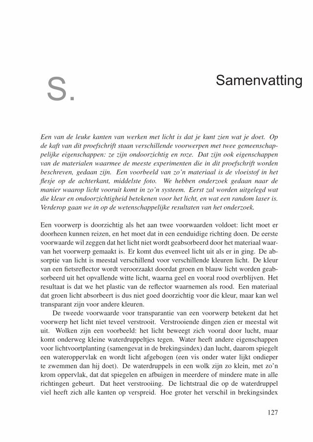
S.Samenvatting
Een van de leuke kanten van werken met licht is dat je kunt zien wat je doet. Opde kaft van dit proefschrift staan verschillende voorwerpen met twee gemeenschap-pelijke eigenschappen: ze zijn ondoorzichtig en roze. Dat zijn ook eigenschappenvan de materialen waarmee de meeste experimenten die in dit proefschrift wordenbeschreven, gedaan zijn. Een voorbeeld van zo’n materiaal is de vloeistof in hetflesje op de achterkant, middelste foto. We hebben onderzoek gedaan naar demanier waarop licht vooruit komt in zo’n systeem. Eerst zal worden uitgelegd watdie kleur en ondoorzichtigheid betekenen voor het licht, en wat een random laser is.Verderop gaan we in op de wetenschappelijke resultaten van het onderzoek.
Een voorwerp is doorzichtig als het aan twee voorwaarden voldoet: licht moet erdoorheen kunnen reizen, en het moet dat in een eenduidige richting doen. De eerstevoorwaarde wil zeggen dat het licht niet wordt geabsorbeerd door het materiaal waar-van het voorwerp gemaakt is. Er komt dus evenveel licht uit als er in ging. De ab-sorptie van licht is meestal verschillend voor verschillende kleuren licht. De kleurvan een fietsreflector wordt veroorzaakt doordat groen en blauw licht worden geab-sorbeerd uit het opvallende witte licht, waarna geel en vooral rood overblijven. Hetresultaat is dat we het plastic van de reflector waarnemen als rood. Een materiaaldat groen licht absorbeert is dus niet goed doorzichtig voor die kleur, maar kan weltransparant zijn voor andere kleuren.
De tweede voorwaarde voor transparantie van een voorwerp betekent dat hetvoorwerp het licht niet teveel verstrooit. Verstrooiende dingen zien er meestal wituit. Wolken zijn een voorbeeld: het licht beweegt zich vooral door lucht, maarkomt onderweg kleine waterdruppeltjes tegen. Water heeft andere eigenschappenvoor lichtvoortplanting (samengevat in de brekingsindex) dan lucht, daarom spiegelteen wateroppervlak en wordt licht afgebogen (een vis onder water lijkt ondieperte zwemmen dan hij doet). De waterdruppels in een wolk zijn zo klein, met zo’nkrom oppervlak, dat dat spiegelen en afbuigen in meerdere of mindere mate in allerichtingen gebeurt. Dat heet verstrooiing. De lichtstraal die op de waterdruppelviel heeft zich alle kanten op verspreid. Hoe groter het verschil in brekingsindex
127
Samenvatting
tussen verstrooier en omgeving, hoe sterker de verstrooiing. Als het licht vaak ver-strooid wordt op de weg door de wolk, dan is het niet meer duidelijk waar het aan debovenkant de wolk in gegaan is. Dit heet veelvoudige verstrooiing en de wolk is danondoorzichtig: we kunnen de zon niet zien. Het licht in de wolk is diffuus. Andereveelvoudig verstrooiende dingen zijn melk of verf.
Het blijkt in de praktijk handiger om licht in zo’n geval niet als een golf, maarals een verzameling deeltjes te beschrijven. Over de individuele deeltjes zeggen weniets, microscopisch bekeken blijft licht een golf. We zijn vooral geınteresseerd inhoeveel van die lichtdeeltjes ergens zijn, de dichtheid. Die blijken we goed te kunnenbeschrijven als diffusie, een erg algemeen transportverschijnsel. Een voorbeeld vandiffusie is de verspreiding van een inktdruppel in een glas water: als de druppel inhet glas valt is er ter plaatse veel inkt en elders niets, maar met het verstrijken van detijd verspreidt de kleur zich door het hele glas, zij het verdund.
We werken met een mengsel van een verstrooiend wit poeder (titaandioxide,hetzelfde pigment dat tandpasta wit maakt) in een rode kleurstof. Het resultaat iseen roze suspensie. De moleculen in de kleurstof absorberen groen licht, vandaarde kleur, en raken daardoor in een aangeslagen toestand. Het groene licht heet de“pomp”. De moleculen hebben de energie uit de pomp in zich opgeslagen, ten kostevan het groene licht. Nu kan de kleurstof rood licht versterken: rood licht dat eenaangeslagen kleurstofmolecuul tegenkomt kan van dat molecuul als het ware eenextra lichtdeeltje meekrijgen waardoor die rode lichtbundel de energie van het mole-cuul overneemt. De kleurstof is dan “roder dan rood”: de kleur ontstaat niet alleendoordat groen licht wordt geabsorbeerd, maar ook door versterking van opvallendrood licht. Een versterkend, verstrooiend materiaal heet een “random laser”.
Lasers maken gebruik van versterking. Normaal gesproken bestaat een laseruit een versterkend medium, bijvoorbeeld zo’n kleurstof, en een zogenaamde “tril-holte”, gevormd door spiegels. De lichtgolf wordt tussen de spiegels heen en weergekaatst, en wordt ondertussen versterkt door de kleurstof. Een van de spiegels isniet perfect reflecterend om de laserbundel uit de trilholte te laten ontsnappen. Als deversterking groot genoeg is (door voldoende te pompen) om het lek door de spiegel tecompenseren is de laser “aan”. De overgang tussen uit en aan heet de laserdrempel.
Er is veel onderzoek gedaan aan lichtvoortplanting in verstrooiende media ennog veel meer aan lasers, zowel voor toepassingen als uit “nieuwsgierigheid”. Onsonderzoek is gedaan uit nieuwsgierigheid. Er zijn twee gezichtspunten op ran-dom lasers te onderscheiden: een vanuit het veld van veelvoudige verstrooiing, eneen vanuit de laserfysica. Er is een duidelijke analogie tussen random en gewonelasers. Gezien vanuit het laser-oogpunt dient zich de vraag aan wat de achter-grond is van deze analogie, waarom twee systemen met zo sterk verschillende op-tische eigenschappen zich soms zo vergelijkbaar gedragen. Aan de andere kant,
128
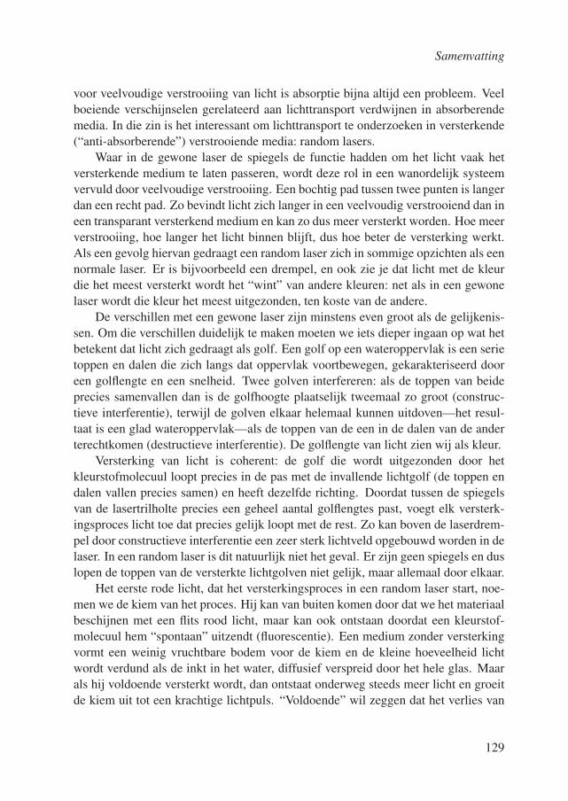
Samenvatting
voor veelvoudige verstrooiing van licht is absorptie bijna altijd een probleem. Veelboeiende verschijnselen gerelateerd aan lichttransport verdwijnen in absorberendemedia. In die zin is het interessant om lichttransport te onderzoeken in versterkende(“anti-absorberende”) verstrooiende media: random lasers.
Waar in de gewone laser de spiegels de functie hadden om het licht vaak hetversterkende medium te laten passeren, wordt deze rol in een wanordelijk systeemvervuld door veelvoudige verstrooiing. Een bochtig pad tussen twee punten is langerdan een recht pad. Zo bevindt licht zich langer in een veelvoudig verstrooiend dan ineen transparant versterkend medium en kan zo dus meer versterkt worden. Hoe meerverstrooiing, hoe langer het licht binnen blijft, dus hoe beter de versterking werkt.Als een gevolg hiervan gedraagt een random laser zich in sommige opzichten als eennormale laser. Er is bijvoorbeeld een drempel, en ook zie je dat licht met de kleurdie het meest versterkt wordt het “wint” van andere kleuren: net als in een gewonelaser wordt die kleur het meest uitgezonden, ten koste van de andere.
De verschillen met een gewone laser zijn minstens even groot als de gelijkenis-sen. Om die verschillen duidelijk te maken moeten we iets dieper ingaan op wat hetbetekent dat licht zich gedraagt als golf. Een golf op een wateroppervlak is een serietoppen en dalen die zich langs dat oppervlak voortbewegen, gekarakteriseerd dooreen golflengte en een snelheid. Twee golven interfereren: als de toppen van beideprecies samenvallen dan is de golfhoogte plaatselijk tweemaal zo groot (construc-tieve interferentie), terwijl de golven elkaar helemaal kunnen uitdoven—het resul-taat is een glad wateroppervlak—als de toppen van de een in de dalen van de anderterechtkomen (destructieve interferentie). De golflengte van licht zien wij als kleur.
Versterking van licht is coherent: de golf die wordt uitgezonden door hetkleurstofmolecuul loopt precies in de pas met de invallende lichtgolf (de toppen endalen vallen precies samen) en heeft dezelfde richting. Doordat tussen de spiegelsvan de lasertrilholte precies een geheel aantal golflengtes past, voegt elk versterk-ingsproces licht toe dat precies gelijk loopt met de rest. Zo kan boven de laserdrem-pel door constructieve interferentie een zeer sterk lichtveld opgebouwd worden in delaser. In een random laser is dit natuurlijk niet het geval. Er zijn geen spiegels en duslopen de toppen van de versterkte lichtgolven niet gelijk, maar allemaal door elkaar.
Het eerste rode licht, dat het versterkingsproces in een random laser start, noe-men we de kiem van het proces. Hij kan van buiten komen door dat we het materiaalbeschijnen met een flits rood licht, maar kan ook ontstaan doordat een kleurstof-molecuul hem “spontaan” uitzendt (fluorescentie). Een medium zonder versterkingvormt een weinig vruchtbare bodem voor de kiem en de kleine hoeveelheid lichtwordt verdund als de inkt in het water, diffusief verspreid door het hele glas. Maarals hij voldoende versterkt wordt, dan ontstaat onderweg steeds meer licht en groeitde kiem uit tot een krachtige lichtpuls. “Voldoende” wil zeggen dat het verlies van
129
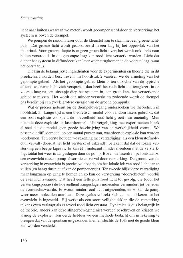
Samenvatting
licht naar buiten (waaraan we meten) wordt gecompenseerd door de versterking: hetsysteem is boven de drempel.
We pompen de random laser door de kleurstof aan te slaan met een groene licht-puls. Dat groene licht wordt geabsorbeerd in een laag bij het oppervlak van hetmateriaal. Voor grotere diepte is er geen groen licht over; het wordt ook deels naarbuiten verstrooid. In die gepompte laag kan rood licht versterkt worden. Licht datdieper het systeem in diffundeert kan later weer terugkomen in de voorste laag, waarhet ontstaan is.
Dit zijn de belangrijkste ingredienten voor de experimenten en theorie die in ditproefschrift worden beschreven. In hoofdstuk 2 varieren we de afmeting van hetgepompte gebied. Als het gepompte gebied klein is ten opzichte van de typischeafstand waarover licht zich verspreidt, dan heeft het rode licht dat terugkeert in devoorste laag na een uitstapje diep het systeem in, een grote kans het versterkendegebied te missen. Het wordt dan minder versterkt en zodoende wordt de drempelpas bereikt bij een (veel) grotere energie van de groene pomppuls.
Wat er precies gebeurt bij de drempelovergang onderzoeken we theoretisch inhoofdstuk 3. Lange tijd is een theoretisch model voor random lasers gebruikt, dateen soort explosie voorspelt: de hoeveelheid rood licht groeit naar oneindig. Mennoemde deze explosie de laserdrempel. Uit vergelijking met experimenten bleekal snel dat dit model geen goede beschrijving van de werkelijkheid vormt. Wepassen dit diffusiemodel op een aantal punten aan, waardoor de explosie kan wordenvoorkomen. Ten eerste houden we rekening met verzadiging: als een kleurstofmole-cuul vervalt (doordat het licht versterkt of uitzendt), betekent dat dat de lokale ver-sterking een beetje lager is. Er kan een molecuul minder meedoen met de versterk-ing, totdat het weer is aangeslagen door de pomp. Boven de laserdrempel ontstaat zoeen evenwicht tussen pomp-absorptie en verval door versterking. De grootte van deversterking in evenwicht is precies voldoende om het lokale lek van rood licht aan tevullen (en hangt dus niet af van de pompenergie). Ten tweede blijkt deze verzadigingmaar langzaam op gang te komen en zo kan de versterking “doorschieten” voorbijde evenwichtswaarde. Dat heeft een felle puls rood licht tot gevolg, die (door hetversterkingsproces) de hoeveelheid aangeslagen moleculen vermindert tot benedende evenwichtswaarde. Er wordt minder rood licht uitgezonden, en zo kan de pompweer meer moleculen aanslaan. Deze cyclus voltrekt zich een aantal keren tot hetevenwicht is ingesteld. Hij werkt als een soort veiligheidsklep die de versterkingtelkens even verlaagt als er teveel rood licht ontstaat. Dynamica is dus belangrijk inde theorie, anders kan deze slingerbeweging niet worden beschreven en krijgen wealsnog de explosie. Ten derde hebben we een methode bedacht om in rekening tebrengen dat van de spontaan uitgezonden kiemen slechts de 10% met de goede kleurkan worden versterkt.
130
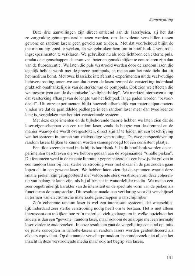
Samenvatting
Deze drie aanvullingen zijn direct ontleend aan de laserfysica, zij het datze zorgvuldig geınterpreteerd moeten worden, om de evidente verschillen tussengewone en random lasers geen geweld aan te doen. Met dat voorbehoud blijkt detheorie nu erg goed te werken, en we gebruiken hem om in hoofdstuk 4 verstrooi-ingsexperimenten te verklaren. We gebruiken nu als rode lichtbron een externe puls,omdat de eigenschappen daarvan veel beter en gemakkelijker te controleren zijn danvan de fluorescentie. We laten die puls verstrooid worden door de random laser, dietegelijk belicht wordt met de groene pomppuls, en meten aan het rode licht dat uithet medium komt. Met twee klassieke interferentie-experimenten uit de veelvoudigelichtverstrooiing tonen we aan dat boven de laserdrempel de versterking inderdaadpraktisch onafhankelijk is van de sterkte van de pomppuls. Ook zien we effecten diewe toeschrijven aan de dynamische “veiligheidsklep”. We merkten hierboven al opdat versterking afhangt van de lengte van het lichtpad: lange paden worden “bevoor-deeld”. Uit onze experimenten blijkt hoeveel: afhankelijk van materiaalparametersvinden we dat de gemiddelde padlengte in een random laser meer dan twee keer zolang is, vergeleken met het niet-versterkende systeem.
Met deze experimenten en de bijbehorende theorie hebben we laten zien dat delaser-eigenschappen van een random laser, zoals de hoogte van de drempel en demanier waarop die wordt overgestoken, direct zijn af te leiden uit een beschrijvingvan het systeem in termen van veelvoudige verstrooiing. De twee perspectieven oprandom lasers blijken te kunnen worden samengevoegd tot een consistent plaatje.
Een tikje vreemde eend in de bijt is hoofdstuk 5. In dit hoofdstuk worden de ex-perimenten beschreven die we hebben gedaan aan de zogenaamde “smalle pieken”.Dit fenomeen werd in de recente literatuur gepresenteerd als een bewijs dat golven ineen random laser bij heel sterke verstrooiing weer met elkaar in de pas zouden gaanlopen als in een gewone laser. We hebben laten zien dat de systemen waarin dezesmalle pieken zijn gerapporteerd niet voldoende sterk verstrooien om deze coheren-tie van belang te laten zijn, als hij al bestaat in wanordelijke media. We meten eenzeer ongebruikelijk karakter van de intensiteit en de spectrale vorm van de pieken alsfunctie van de pompsterkte. Dit resultaat maakt een verklaring voor dit verschijnselin termen van electronische materiaaleigenschappen waarschijnlijker.
Zo’n coherente random laser is wel een interessant systeem, dat waarschijn-lijk inderdaad zeer sterke verstrooiing nodig heeft om te bestaan. Het is niet alleeninteressant om te kijken hoe zo’n materiaal zich gedraagt en in welke opzichten hetanders is dan een “gewone” random laser, maar ook om de analogie met een normalelaser verder te onderzoeken. In onze resultaten gaat de vergelijking een eind op, mitsde juiste concepten in trilholte-lasers en random lasers worden geıdentificeerd alselkaars equivalent. Op die manier verscherpt random-laseronderzoek niet alleen hetinzicht in deze verstrooiende media maar ook het begrip van lasers.
131

D.Dankwoord
Iedereen die direct of indirect, doelgericht of onbewust heeft bijgedragen aan hetwerk dat in dit boek beschreven is ben ik zeer erkentelijk. Wetenschap bedrijf je nietalleen. Ook al zit je avonden in je eentje te meten, ideeen worden gevormd onderde continue invloed van je omgeving. Daarmee bedoel ik niet alleen invloed vancollega’s die slimme vragen stellen, maar ook van anderen waarvan ik gewoon blijben dat ze er zijn. Een aantal van hen wil ik hier met name noemen.
Allereerst dank ik mijn promotor Ad Lagendijk, die alles aan de kant zet omwetenschap te kunnen doen, voor het gestelde vertrouwen, zowel wat betreft dewetenschappelijke als de sociale kanten van het onderzoek. Ook zijn aanstekelijkenthousiasme voor en heldere kijk op de natuurkunde waardeer ik zeer. Rudolf Sprikdank ik voor de hulp bij het rekenwerk, zonder hem was ik in hoofdstuk 3 en 4 vandit proefschrift niet zo ver gekomen. Ook heeft hij het talent om alle mogelijke berenop de weg te signaleren als je een idee voor een experiment hebt. Als die allemaalzijn afgeschoten kan er zeker niets meer mis gaan. Willem Vos en Gerard Wegdamdank ik voor de niet aflatende stroom van ideetjes waarvan ik er veel te weinig ge-bruikt heb. Zorro, you are what you is, bedankt voor alles. Gerard, ik hoop dat je jebetrokkenheid niet hoeft te bekopen met een lange periode als instituutsdirecteur.
I am very grateful to Makoto Tomita for his patience and lessons in setting upexperiments. The beam diameter experiment and the following collaboration gaveme a good start in random lasers. Mijn afstudeerstudent Frank J. Poelwijk dankik voor zijn optimisme en zijn oog voor detail in experimenten. Frank, ik bewaarmooie herinneringen aan onze discussies, zowel over random lasers als over filosofie,moderne muziek en wie weet wat nog meer. Het was inderdaad een goede tijd.
Waar zouden we zijn zonder Wim Koops? Ik bedank hem niet alleen voor detechnische, maar ook voor de morele ondersteuning: zijn interesse in de mens achterde wetenschapper, zijn schaatsverhalen en zijn trots als opa.
Zonder de techniek draait er natuurlijk niets in een experimenteel lab. BedanktJohan van de Ridder (ook voor je onverwoestbare humeur), Flip de Leeuw en JoostOvertoom (ook voor de labborrels—zo hoor je nog eens wat), Johan Soede, JanDekker, Jan Mulder en Bert Zwart, voor alle snelle klusjes “even tussendoor”. Dank
133
Dankwoord
aan Ina Zwart, Ineke Baaij, Roos Visser en Mariet Bos voor de vlotte administratieveen secretariele ondersteuning. Als er haast is bij de financien weet Dick Jensen hetaltijd te regelen. Derk Bouhuijs en Marc Brugman tilden de computersupport naareen hoger plan.
Frederik van den Broek en Huib Bakker van Amolf sloten zich voor een dagaan bij de zoektocht naar de smalle pieken. Niets gezien, maar wel bedankt voor dehulp en het gebruik van de laser. The attempt with Nandini Bhattacharya’s setup wasa little more successful, and I thank her for her help and for tolerating my stuff inthe lab for a week. Wat het probleem ook is, Cor Snoek heeft de oplossing te leen,bouwjaar ca. 1965, maar werkt geheid en je krijgt er mooie verhalen bij.
The curiosity of Diederik Wiersma, Bart van Tiggelen, Jos Dingjan and CostasSoukoulis gave rise to inspiring discussions and ideas on random lasers and localiza-tion. I am indebted to Claude Weisbuch for illuminating the tricky subject of II–VIluminescence. Dank aan Ben van Linden van den Heuvell voor zijn belangstelling.Hans Pothuizen, bedankt voor de aanmoediging en je kritische blik.
In de groep Golven in Complexe Media is altijd beweging. Dat is inspirerenden leuk. Bedankt Jaime, poldercharro en partner in wanorde, voor wederzijdse be-moeienis, vrijmibo’s en AC/DC, Patrick voor de rake vragen, Martijn die zeker werktin theorie, Yuri, Juan para los intercambios de idiomas y toda la musica, Electron-transFemius tegen wil en dank, Manu, kamergenoot op de valreep Boris, Lydia voorde roze spullen, Denis, Tom, Bert, Rik, Mark, Frank voor de lol, de rust en dewilde plannen, Mischa voor zijn ongeduld en de vele uitjes, Dirk! ( . . . ja?), Ju-dith voor haar eigenwijsheid, Pedro, de Canadezen Hendrik en Henk, Michiel voorde inzichten van buiten, Arnout, Dau, Dennis, Anouk, Meritt, Pepijn en Allard.
Aan de lotgenoten buiten de groep, zoals Erik Paul, Bas, Michel, Jeroen, Heidi,Lunterense kamergenoot Dirk en β-stuffel Ronald, dank voor hetzelfde schuitje.
Susanne, bestaat er zoiets als een copromovendus? Zonder jou had mijn tijd inAmsterdam er heel anders uitgezien, ik ben erg blij dat je er was. Roelof, dank voorde lange avonden (met nachtnet toe) en de gesprekken over leven en werk, zin enonzin. Marij, bedankt voor je steun, vriendschap en de leuke tijd, Kirsten voor jebetrokkenheid, Miranda voor de hulp bij het grafisch ontwerp van dit boek, Rick,Jos en Raymond voor het kabaal, de lol en de rare instrumenten, Thomas voor zijnenthousiasme en de muziek.
De family, Joost, Floor, Francien en Erik, pap en mam, dank voor de steun enaanmoediging en de goede zorgen. Francien, ook bedankt voor de frustitelefoontjes.Tot slot, lieve Suze, je vertrouwen en je praktische instelling in situaties waarin ikhet overzicht verloor, zijn ontzettend waardevol geweest in dat toch wel zware laatstejaar. Kom, we gaan de wereld in!
Gijs
134


![Nanoparticle-doped electrospun fiber random lasers with ... · [2,6,8,10]. Organic crystals [16,17] and epitaxial nanowires [18], biopolymers [19,20], as well as conjugated polymers](https://img.pdfslide.tips/doc/110x75/600d3d88f8e5ef616721ea08/nanoparticle-doped-electrospun-fiber-random-lasers-with-26810-organic.jpg)


![Karimi understanding lasers[1]](https://img.pdfslide.tips/doc/110x75/587df0b41a28abab7e8b4bfd/karimi-understanding-lasers1.jpg)