EXTREME VALUE THEORY

Richard L. Smith

Department of Statistics and Operations Research

University of North Carolina

Chapel Hill, NC 27599-3260

rls@email.unc.edu

AMS Committee on Probability and Statistics

Short Course on Statistics of Extreme Events

Phoenix, January 11, 2009

1

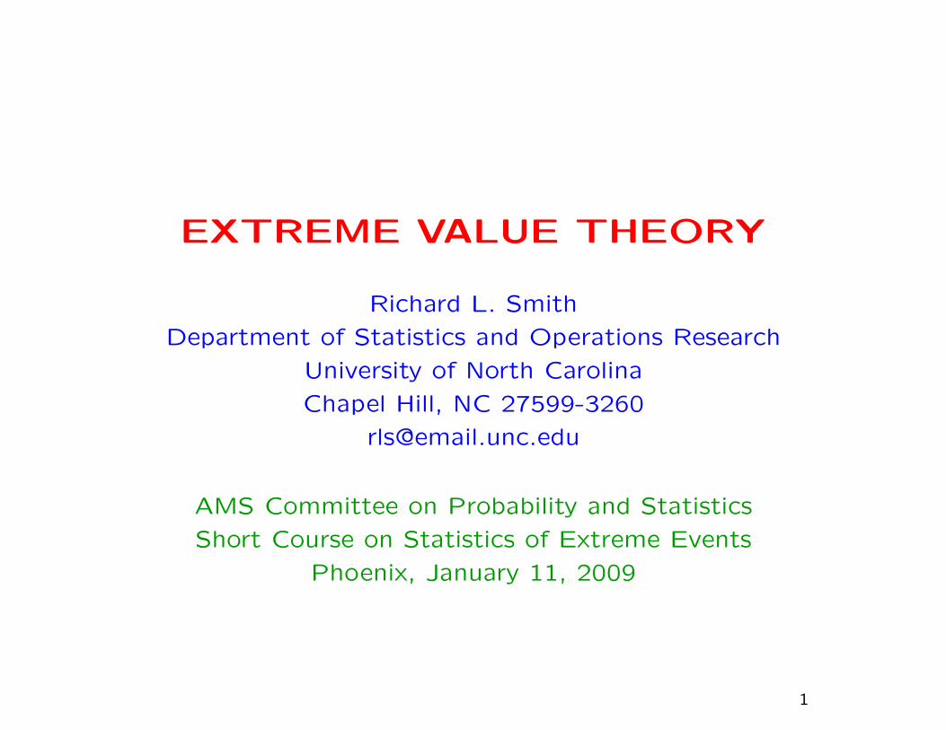
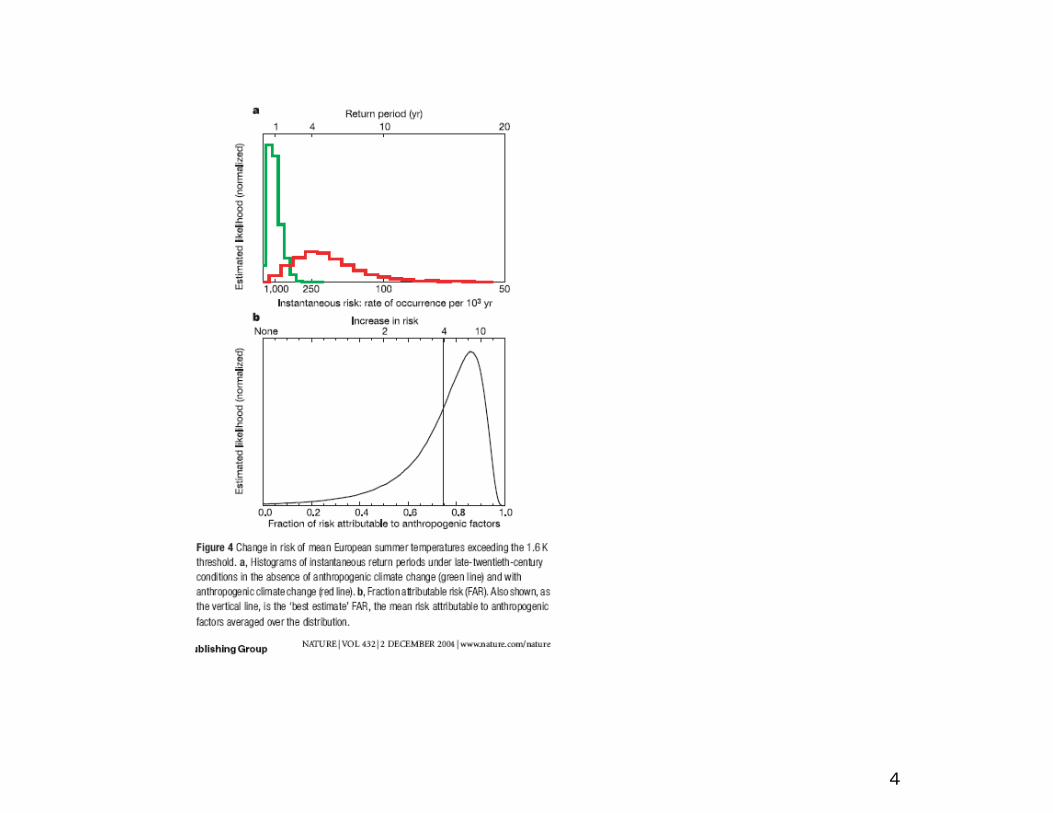
(From a presentation by Myles Allen)

2

3

4

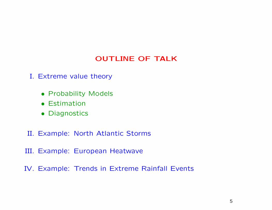
OUTLINE OF TALK

I. Extreme value theory

• Probability Models

• Estimation

• Diagnostics

II. Example: North Atlantic Storms

III. Example: European Heatwave

IV. Example: Trends in Extreme Rainfall Events

5

I. EXTREME VALUE THEORY

6

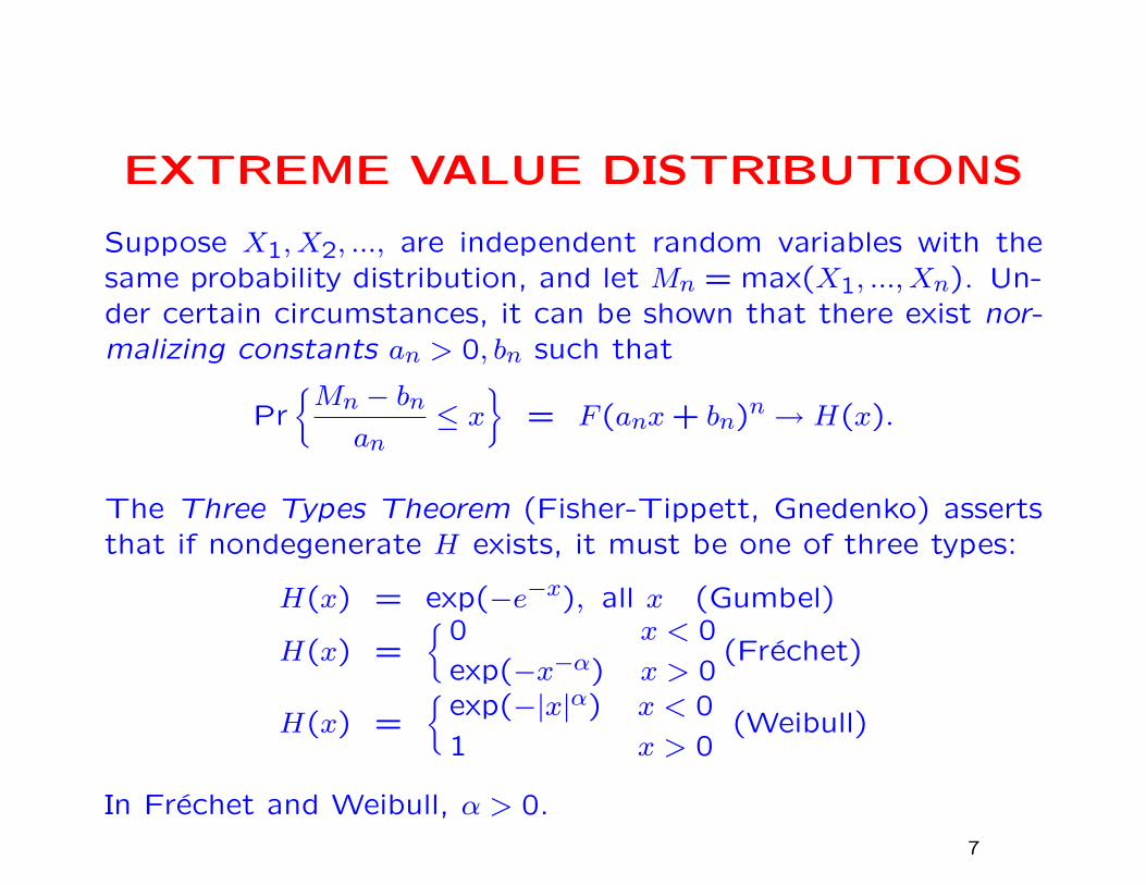
EXTREME VALUE DISTRIBUTIONS

Suppose X1, X2, ..., are independent random variables with thesame probability distribution, and let Mn = max(X1, ..., Xn). Un-der certain circumstances, it can be shown that there exist nor-malizing constants an > 0, bn such that

Pr{Mn − bnan

≤ x}

= F (anx+ bn)n → H(x).

The Three Types Theorem (Fisher-Tippett, Gnedenko) assertsthat if nondegenerate H exists, it must be one of three types:

H(x) = exp(−e−x), all x (Gumbel)

H(x) ={0 x < 0

exp(−x−α) x > 0(Frechet)

H(x) ={

exp(−|x|α) x < 0

1 x > 0(Weibull)

In Frechet and Weibull, α > 0.

7

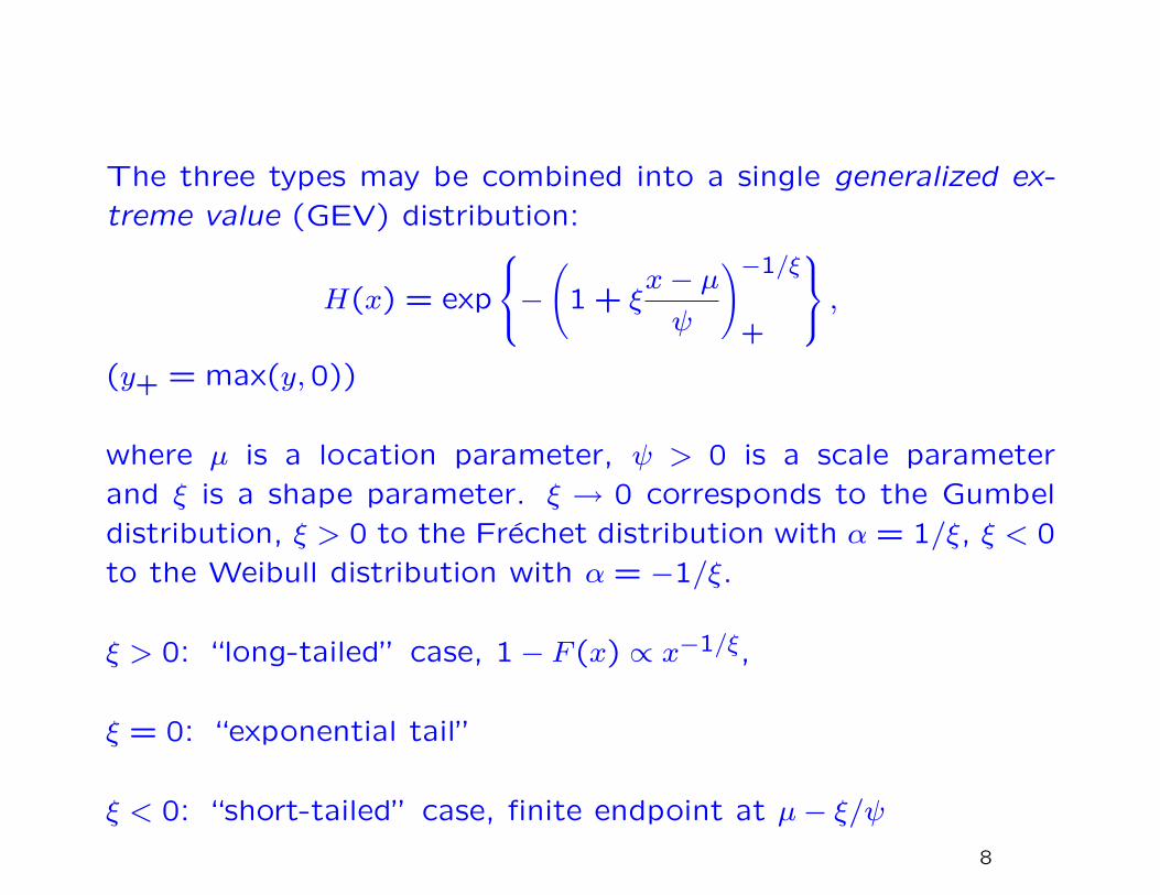
The three types may be combined into a single generalized ex-

treme value (GEV) distribution:

H(x) = exp

−(

1 + ξx− µψ

)−1/ξ

+

,(y+ = max(y,0))

where µ is a location parameter, ψ > 0 is a scale parameter

and ξ is a shape parameter. ξ → 0 corresponds to the Gumbel

distribution, ξ > 0 to the Frechet distribution with α = 1/ξ, ξ < 0

to the Weibull distribution with α = −1/ξ.

ξ > 0: “long-tailed” case, 1− F (x) ∝ x−1/ξ,

ξ = 0: “exponential tail”

ξ < 0: “short-tailed” case, finite endpoint at µ− ξ/ψ8

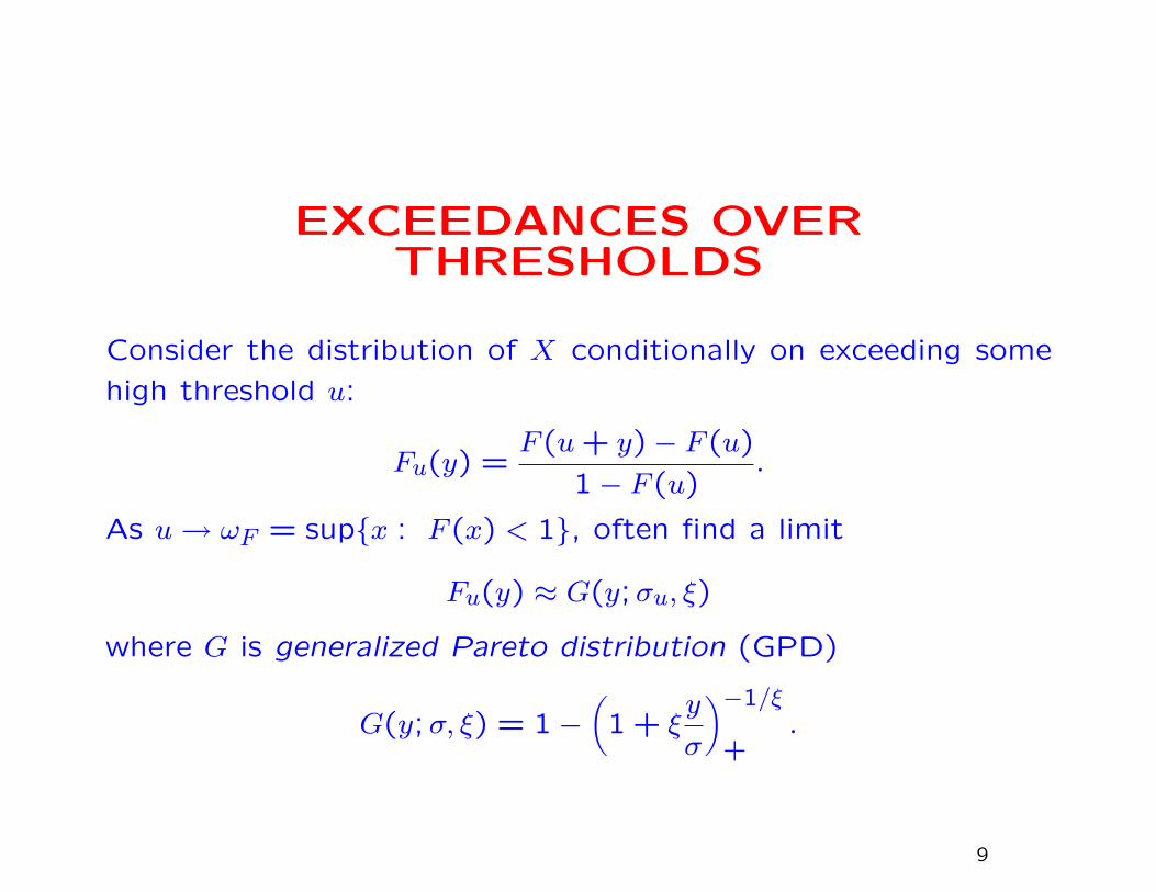
EXCEEDANCES OVERTHRESHOLDS

Consider the distribution of X conditionally on exceeding some

high threshold u:

Fu(y) =F (u+ y)− F (u)

1− F (u).

As u→ ωF = sup{x : F (x) < 1}, often find a limit

Fu(y) ≈ G(y;σu, ξ)

where G is generalized Pareto distribution (GPD)

G(y;σ, ξ) = 1−(

1 + ξy

σ

)−1/ξ

+.

9

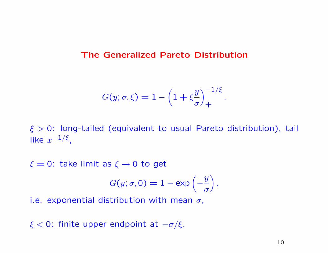
The Generalized Pareto Distribution

G(y;σ, ξ) = 1−(

1 + ξy

σ

)−1/ξ

+.

ξ > 0: long-tailed (equivalent to usual Pareto distribution), tail

like x−1/ξ,

ξ = 0: take limit as ξ → 0 to get

G(y;σ,0) = 1− exp(−y

σ

),

i.e. exponential distribution with mean σ,

ξ < 0: finite upper endpoint at −σ/ξ.

10

The Poisson-GPD model combines the GPD for the excesses

over the threshold with a Poisson distribtion for the number of

exceedances. Usually the mean of the Poisson distribution is

taken to be λ per unit time.

11

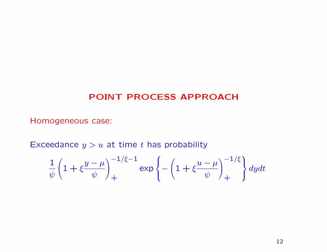
POINT PROCESS APPROACH

Homogeneous case:

Exceedance y > u at time t has probability

1

ψ

(1 + ξ

y − µψ

)−1/ξ−1

+exp

−(

1 + ξu− µψ

)−1/ξ

+

dydt

12

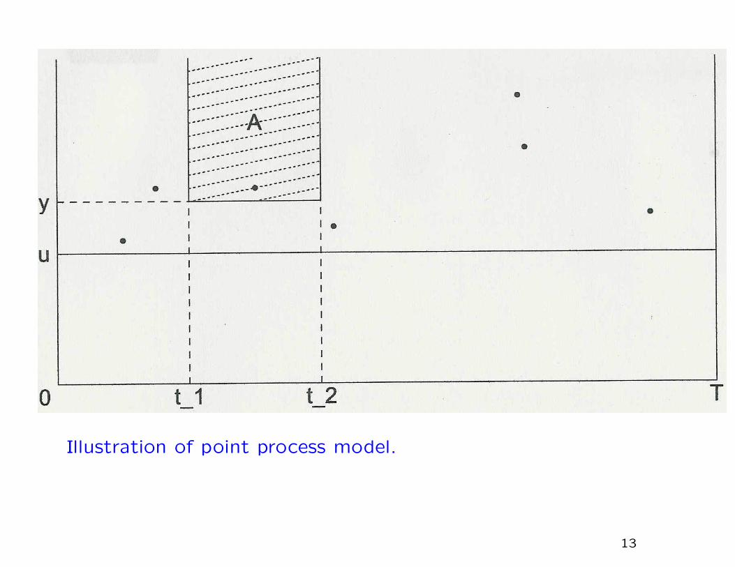
Illustration of point process model.

13

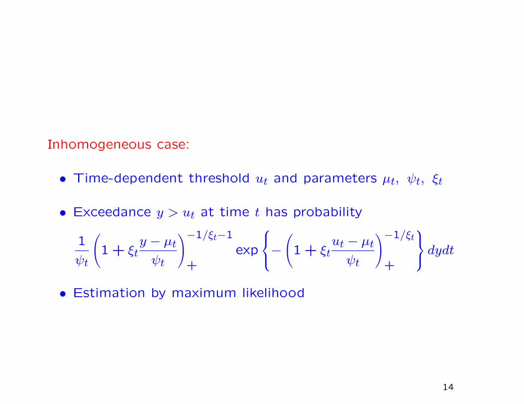
Inhomogeneous case:

• Time-dependent threshold ut and parameters µt, ψt, ξt

• Exceedance y > ut at time t has probability

1

ψt

(1 + ξt

y − µtψt

)−1/ξt−1

+exp

−(

1 + ξtut − µtψt

)−1/ξt

+

dydt• Estimation by maximum likelihood

14

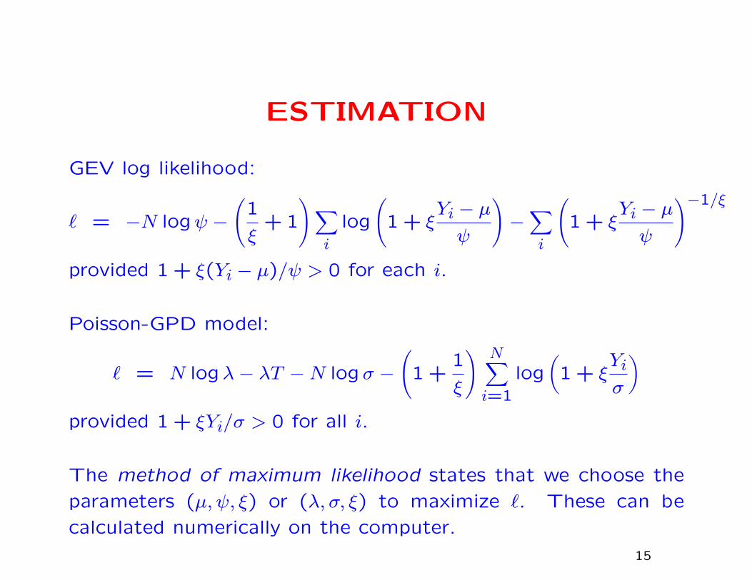
ESTIMATION

GEV log likelihood:

` = −N logψ −(

1

ξ+ 1

)∑i

log

(1 + ξ

Yi − µψ

)−∑i

(1 + ξ

Yi − µψ

)−1/ξ

provided 1 + ξ(Yi − µ)/ψ > 0 for each i.

Poisson-GPD model:

` = N logλ− λT −N logσ −(

1 +1

ξ

) N∑i=1

log(

1 + ξYiσ

)provided 1 + ξYi/σ > 0 for all i.

The method of maximum likelihood states that we choose the

parameters (µ, ψ, ξ) or (λ, σ, ξ) to maximize `. These can be

calculated numerically on the computer.

15

DIAGNOSTICS

Gumbel plots

QQ plots of residuals

Mean excess plot

Z and W plots

16

Gumbel plots

Used as a diagnostic for Gumbel distribution with annual maxima

data. Order data as Y1:N ≤ ... ≤ YN :N , then plot Yi:N against

reduced value xi:N ,

xi:N = − log(− log pi:N),

pi:N being the i’th plotting position, usually taken to be (i−12)/N .

A straight line is ideal. Curvature may indicate Frechet or Weibull

form. Also look for outliers.

17

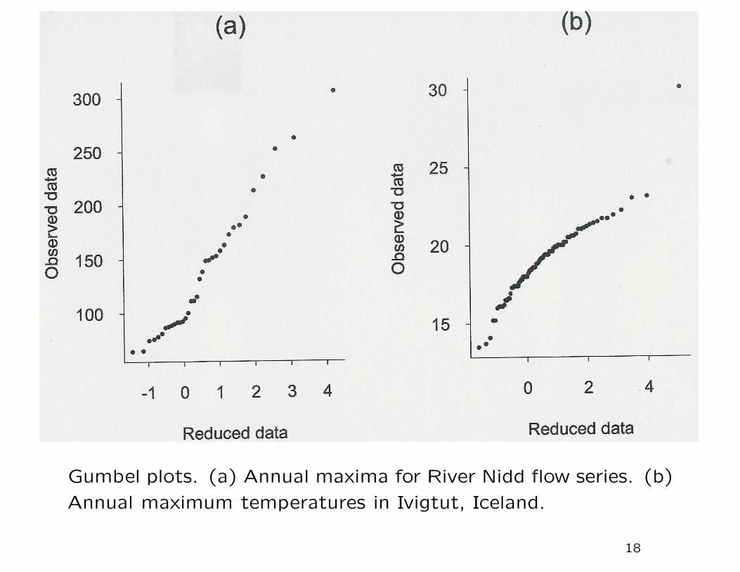
Gumbel plots. (a) Annual maxima for River Nidd flow series. (b)

Annual maximum temperatures in Ivigtut, Iceland.

18

QQ plots of residuals

A second type of probability plot is drawn after fitting the model.

Suppose Y1, ..., YN are IID observations whose common distribu-

tion function is G(y; θ) depending on parameter vector θ. Sup-

pose θ has been estimated by θ, and let G−1(p; θ) denote the

inverse distribution function of G, written as a function of θ. A

QQ (quantile-quantile) plot consists of first ordering the obser-

vations Y1:N ≤ ... ≤ YN :N , and then plotting Yi:N against the

reduced value

xi:N = G−1(pi:N ; θ),

where pi:N may be taken as (i− 12)/N . If the model is a good fit,

the plot should be roughly a straight line of unit slope through

the origin.

Examples...

19

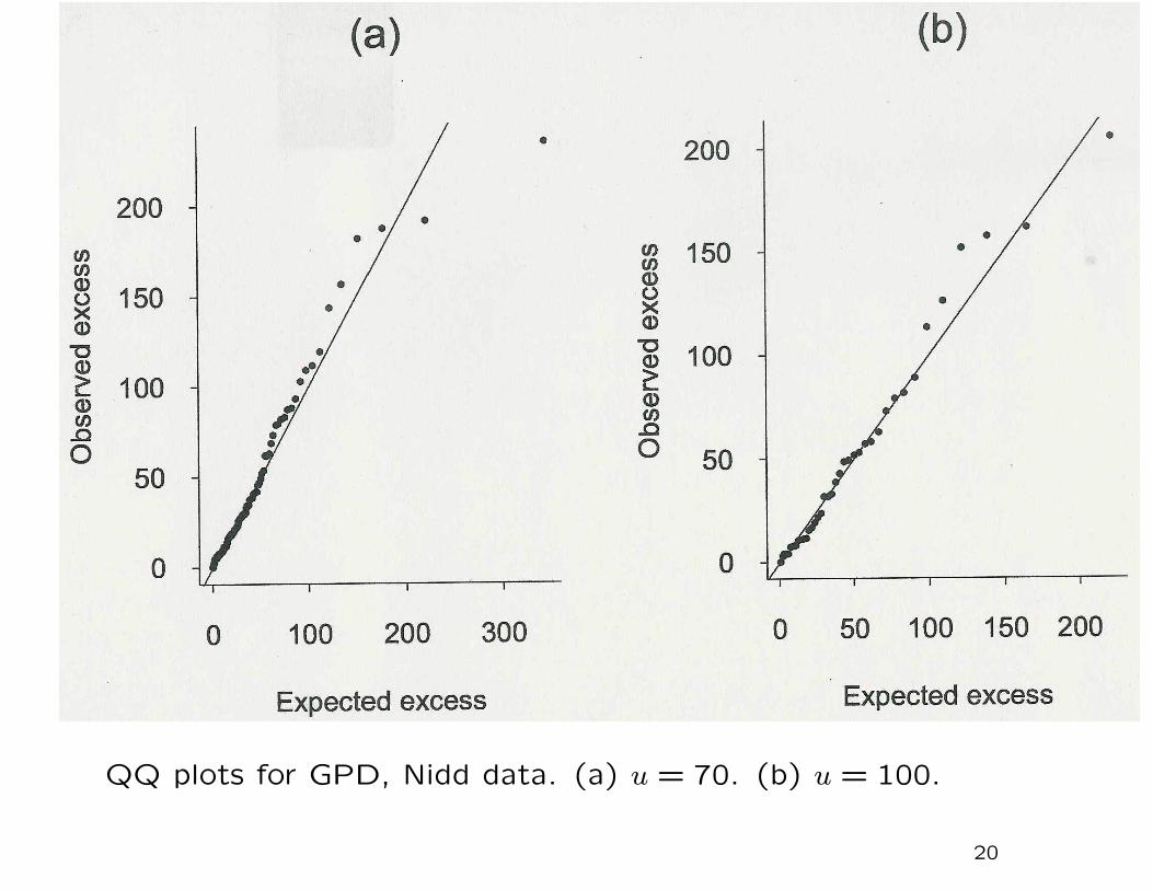
QQ plots for GPD, Nidd data. (a) u = 70. (b) u = 100.

20

Mean excess plot

Idea: for a sequence of values of w, plot the mean excess over

w against w itself. If the GPD is a good fit, the plot should be

approximately a straight line.

In practice, the actual plot is very jagged and therefore its “straight-

ness” is difficult to assess. However, a Monte Carlo technique,

assuming the GPD is valid throughout the range of the plot, can

be used to assess this.

Examples...

21

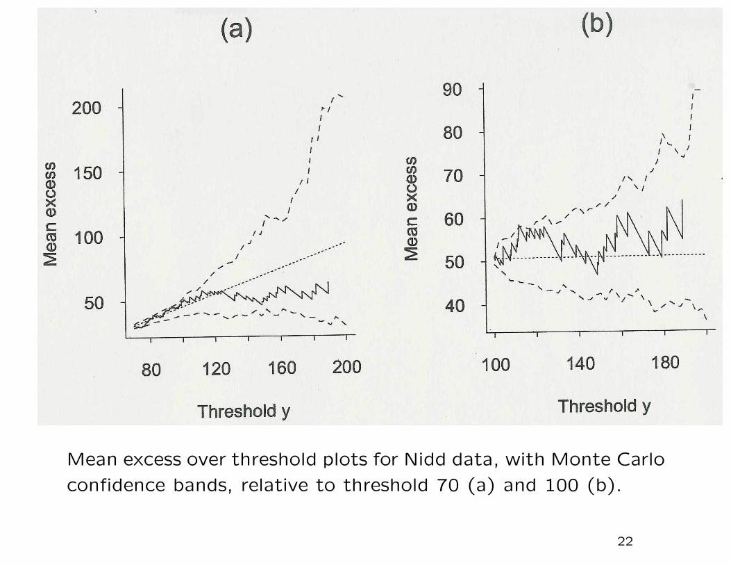
Mean excess over threshold plots for Nidd data, with Monte Carlo

confidence bands, relative to threshold 70 (a) and 100 (b).

22

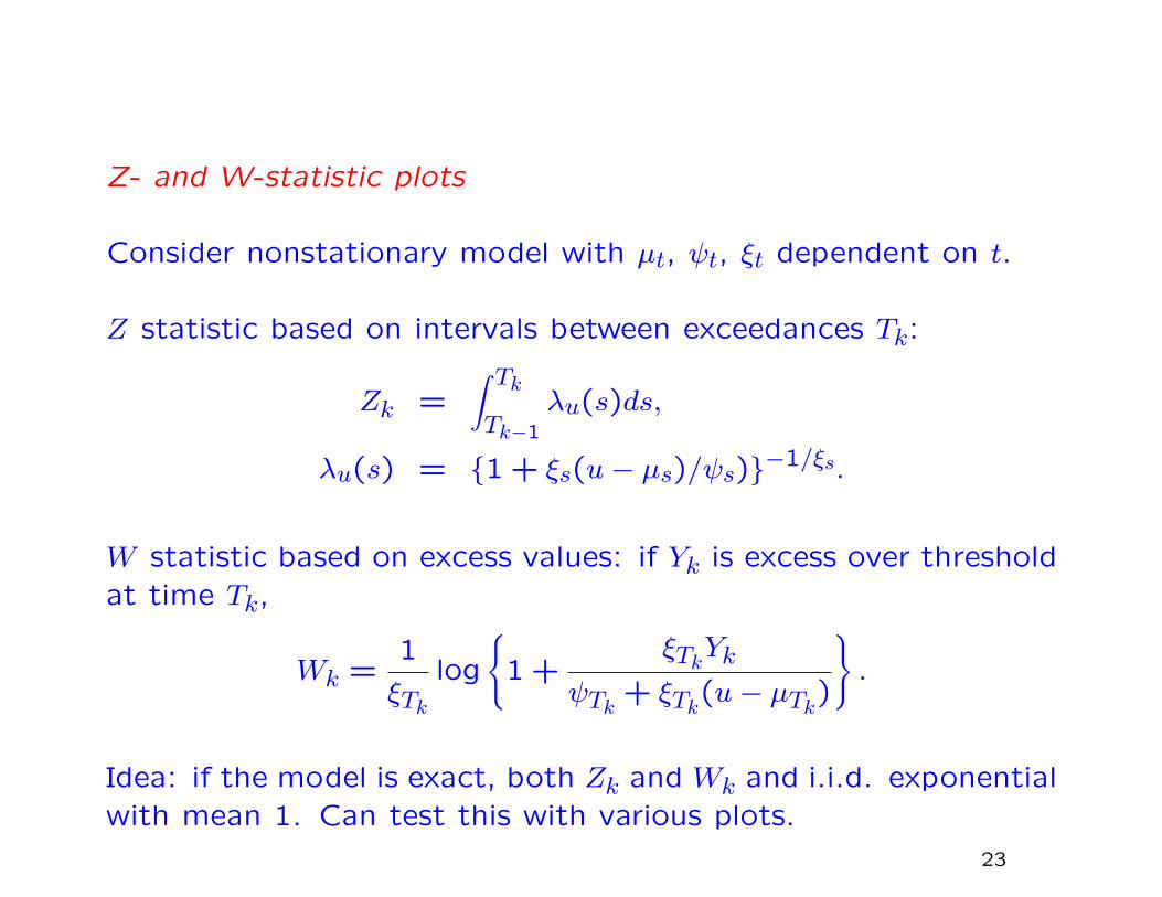
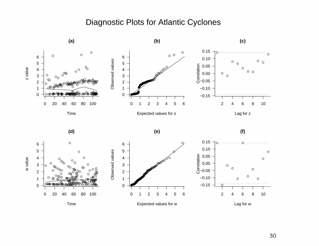
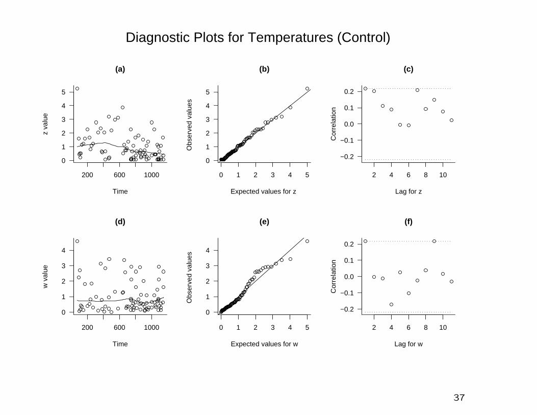
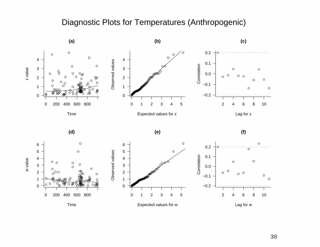
Z- and W-statistic plots

Consider nonstationary model with µt, ψt, ξt dependent on t.

Z statistic based on intervals between exceedances Tk:

Zk =∫ TkTk−1

λu(s)ds,

λu(s) = {1 + ξs(u− µs)/ψs)}−1/ξs.

W statistic based on excess values: if Yk is excess over thresholdat time Tk,

Wk =1

ξTklog

{1 +

ξTkYk

ψTk + ξTk(u− µTk)

}.

Idea: if the model is exact, both Zk and Wk and i.i.d. exponentialwith mean 1. Can test this with various plots.

23

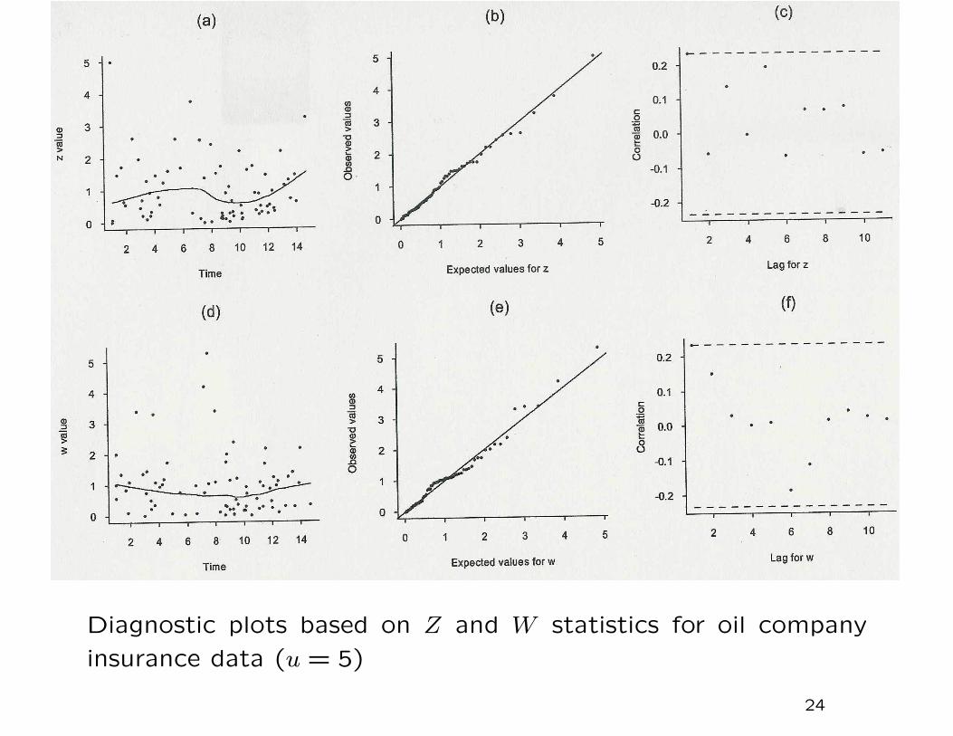
Diagnostic plots based on Z and W statistics for oil company

insurance data (u = 5)

24

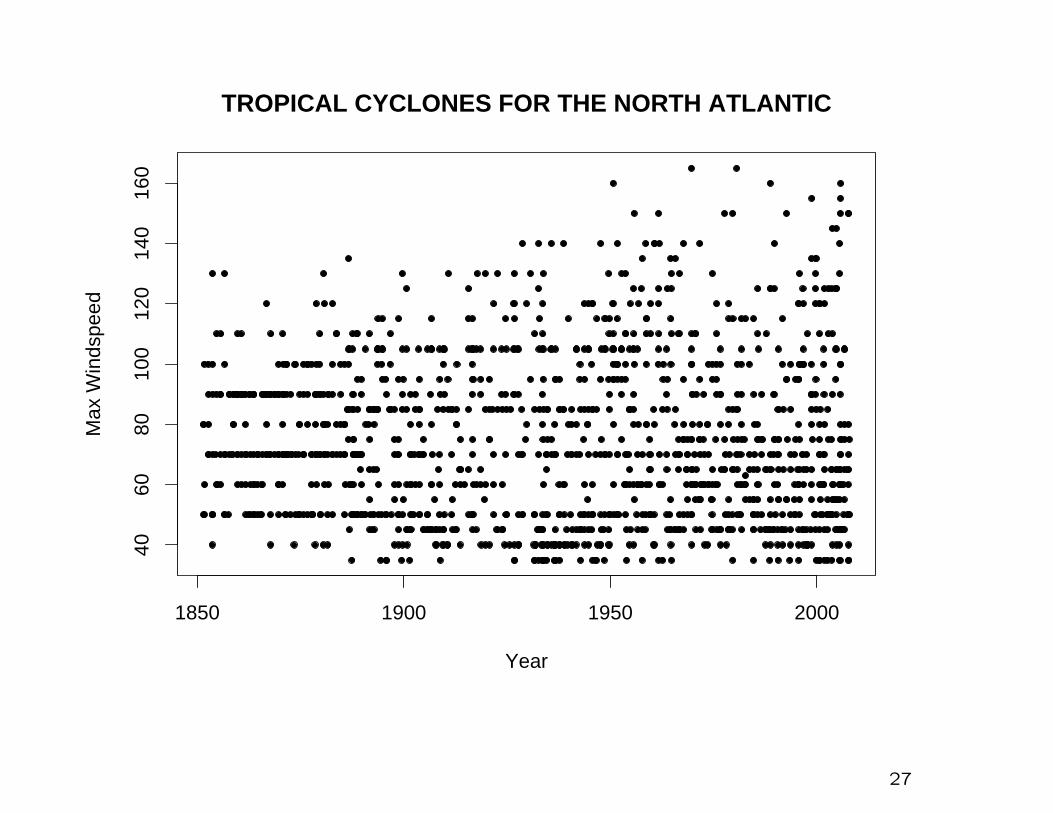
II. NORTH ATLANTIC CYCLONES

25

Data from HURDAT

Maximum windspeeds in all North Atlantic Cyclones from 1851–

2007

26

1850 1900 1950 2000

4060

8010

012

014

016

0

TROPICAL CYCLONES FOR THE NORTH ATLANTIC

Year

Max

Win

dspe

ed

27

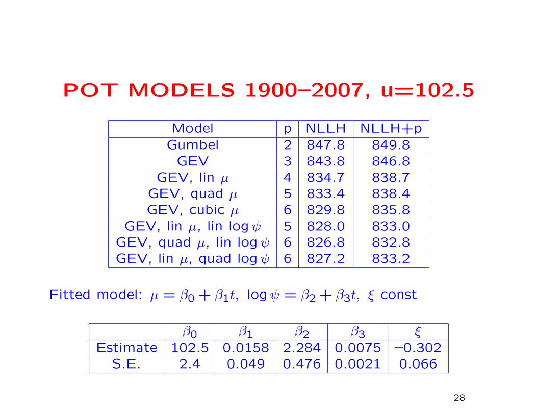
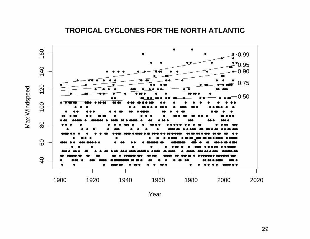
POT MODELS 1900–2007, u=102.5

Model p NLLH NLLH+pGumbel 2 847.8 849.8

GEV 3 843.8 846.8GEV, lin µ 4 834.7 838.7

GEV, quad µ 5 833.4 838.4GEV, cubic µ 6 829.8 835.8

GEV, lin µ, lin logψ 5 828.0 833.0GEV, quad µ, lin logψ 6 826.8 832.8GEV, lin µ, quad logψ 6 827.2 833.2

Fitted model: µ = β0 + β1t, logψ = β2 + β3t, ξ const

β0 β1 β2 β3 ξEstimate 102.5 0.0158 2.284 0.0075 –0.302

S.E. 2.4 0.049 0.476 0.0021 0.066

28

1900 1920 1940 1960 1980 2000 2020

4060

8010

012

014

016

0

TROPICAL CYCLONES FOR THE NORTH ATLANTIC

Year

Max

Win

dspe

ed

0.50

0.75

0.900.95

0.99

29

0 20 40 60 80 100

0

1

2

3

4

5

6

(a)

Time

z va

lue

0 1 2 3 4 5 6

0

1

2

3

4

5

6

(b)

Expected values for z O

bser

ved

valu

es

2 4 6 8 10

−0.15

−0.10

−0.05

0.00

0.05

0.10

0.15

(c)

Lag for z

Cor

rela

tion

0 20 40 60 80 100

0

1

2

3

4

5

6

(d)

Time

w v

alue

0 1 2 3 4 5 6

0

1

2

3

4

5

6

(e)

Expected values for w

Obs

erve

d va

lues

2 4 6 8 10

−0.15

−0.10

−0.05

0.00

0.05

0.10

0.15

(f)

Lag for w

Cor

rela

tion

Diagnostic Plots for Atlantic Cyclones

30

III. EUROPEAN HEATWAVE

31

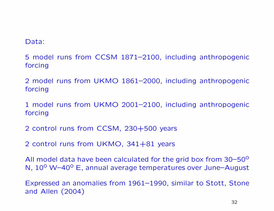
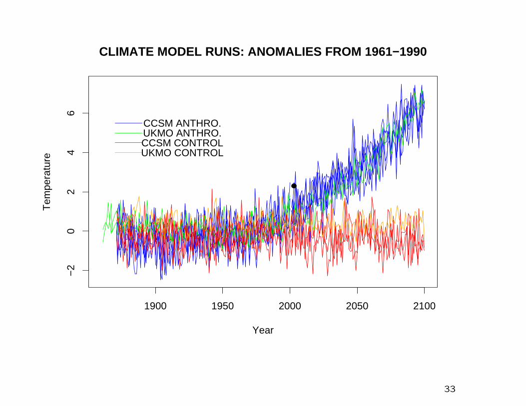
Data:

5 model runs from CCSM 1871–2100, including anthropogenicforcing

2 model runs from UKMO 1861–2000, including anthropogenicforcing

1 model runs from UKMO 2001–2100, including anthropogenicforcing

2 control runs from CCSM, 230+500 years

2 control runs from UKMO, 341+81 years

All model data have been calculated for the grid box from 30–50o

N, 10o W–40o E, annual average temperatures over June–August

Expressed an anomalies from 1961–1990, similar to Stott, Stoneand Allen (2004)

32

1900 1950 2000 2050 2100

−2

02

46

CLIMATE MODEL RUNS: ANOMALIES FROM 1961−1990

Year

Tem

pera

ture

CCSM CONTROL

CCSM ANTHRO.

UKMO CONTROL

UKMO ANTHRO.

33

Method:

Fit POT models with various trend terms to the anthropogenic

model runs, 1861–2010

Also fit trend-free model to control runs (µ = 0.176, logψ =

−1.068, ξ = −0.068)

34

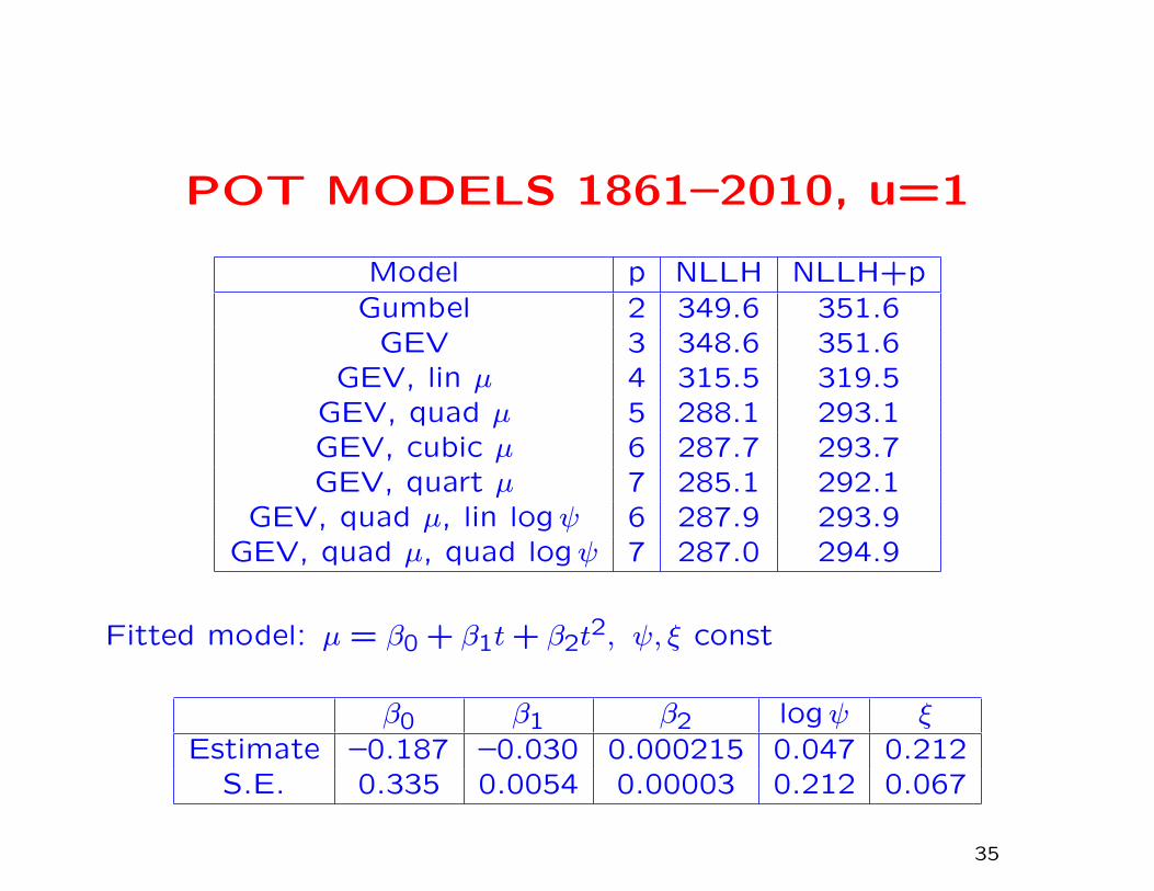
POT MODELS 1861–2010, u=1

Model p NLLH NLLH+pGumbel 2 349.6 351.6

GEV 3 348.6 351.6GEV, lin µ 4 315.5 319.5

GEV, quad µ 5 288.1 293.1GEV, cubic µ 6 287.7 293.7GEV, quart µ 7 285.1 292.1

GEV, quad µ, lin logψ 6 287.9 293.9GEV, quad µ, quad logψ 7 287.0 294.9

Fitted model: µ = β0 + β1t+ β2t2, ψ, ξ const

β0 β1 β2 logψ ξEstimate –0.187 –0.030 0.000215 0.047 0.212

S.E. 0.335 0.0054 0.00003 0.212 0.067

35

1900 1950 2000

−2

02

46

CLIMATE MODEL RUNS: ANOMALIES FROM 1961−1990

Year

Tem

pera

ture

CCSM CONTROL

CCSM ANTHRO.

UKMO CONTROL

UKMO ANTHRO.

90 %99 %90 %

99 %

36

200 600 1000

0

1

2

3

4

5

(a)

Time

z va

lue

0 1 2 3 4 5

0

1

2

3

4

5

(b)

Expected values for z O

bser

ved

valu

es

2 4 6 8 10

−0.2

−0.1

0.0

0.1

0.2

(c)

Lag for z

Cor

rela

tion

200 600 1000

0

1

2

3

4

(d)

Time

w v

alue

0 1 2 3 4 5

0

1

2

3

4

(e)

Expected values for w

Obs

erve

d va

lues

2 4 6 8 10

−0.2

−0.1

0.0

0.1

0.2

(f)

Lag for w

Cor

rela

tion

Diagnostic Plots for Temperatures (Control)

37

0 200 400 600 800

0

1

2

3

4

(a)

Time

z va

lue

0 1 2 3 4 5

0

1

2

3

4

(b)

Expected values for z O

bser

ved

valu

es

2 4 6 8 10

−0.2

−0.1

0.0

0.1

0.2

(c)

Lag for z

Cor

rela

tion

0 200 400 600 800

0

1

2

3

4

5

6

(d)

Time

w v

alue

0 1 2 3 4 5

0

1

2

3

4

5

6

(e)

Expected values for w

Obs

erve

d va

lues

2 4 6 8 10

−0.2

−0.1

0.0

0.1

0.2

(f)

Lag for w

Cor

rela

tion

Diagnostic Plots for Temperatures (Anthropogenic)

38

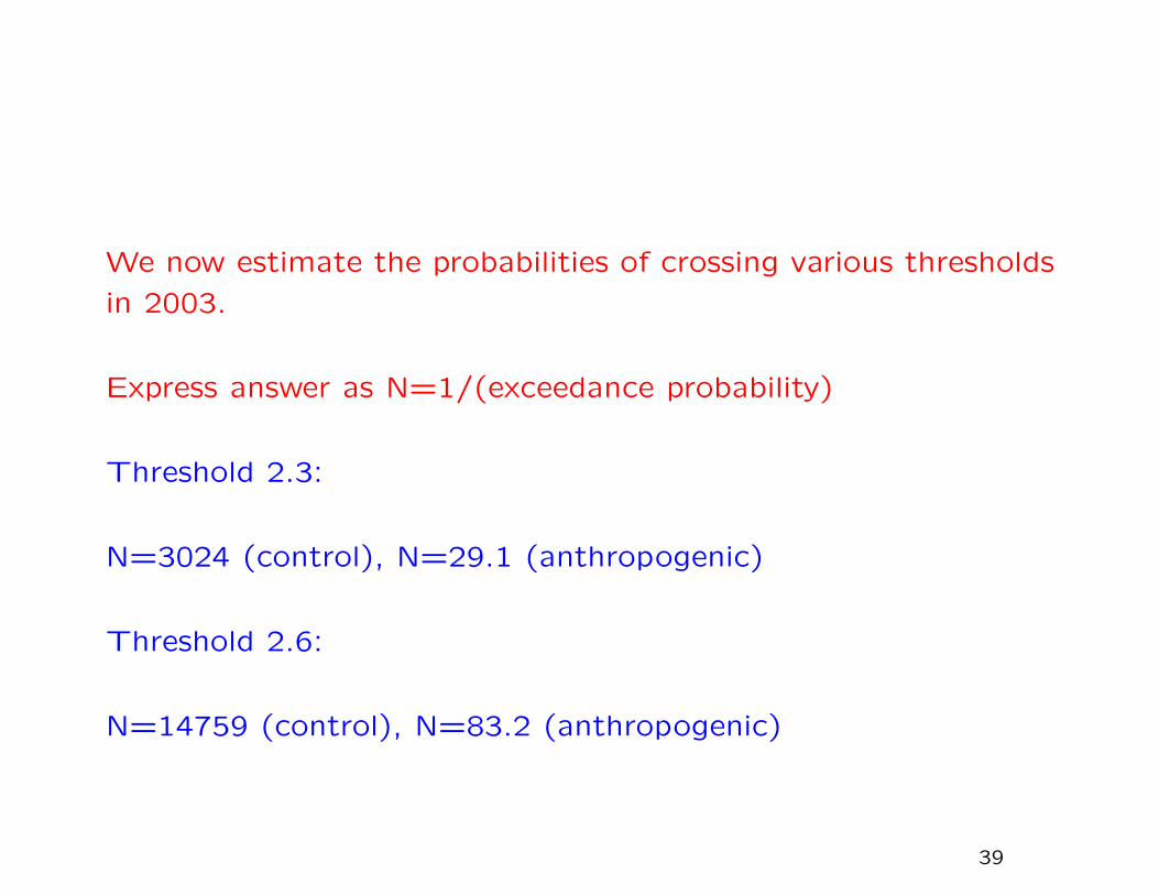
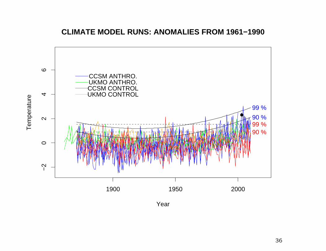
We now estimate the probabilities of crossing various thresholds

in 2003.

Express answer as N=1/(exceedance probability)

Threshold 2.3:

N=3024 (control), N=29.1 (anthropogenic)

Threshold 2.6:

N=14759 (control), N=83.2 (anthropogenic)

39

IV. TREND IN PRECIPITATIONEXTREMES

(joint work with Amy Grady and Gabi Hegerl)

During the past decade, there has been extensive research byclimatologists documenting increases in the levels of extremeprecipitation, but in observational and model-generated data.

With a few exceptions (papers by Katz, Zwiers and co-authors)this literature have not made use of the extreme value distribu-tions and related constructs

There are however a few papers by statisticians that have ex-plored the possibility of using more advanced extreme valuemethods (e.g. Cooley, Naveau and Nychka, to appear JASA;Sang and Gelfand, submitted)

This discussion uses extreme value methodology to look fortrends

40

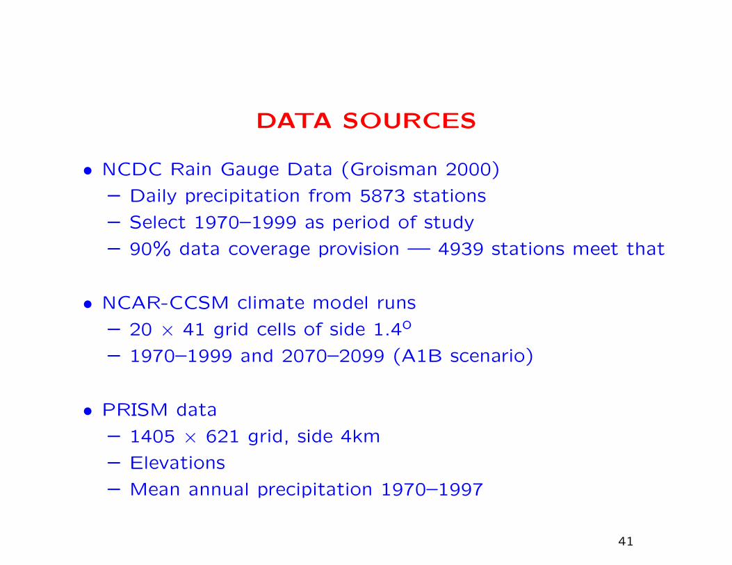
DATA SOURCES

• NCDC Rain Gauge Data (Groisman 2000)

– Daily precipitation from 5873 stations

– Select 1970–1999 as period of study

– 90% data coverage provision — 4939 stations meet that

• NCAR-CCSM climate model runs

– 20 × 41 grid cells of side 1.4o

– 1970–1999 and 2070–2099 (A1B scenario)

• PRISM data

– 1405 × 621 grid, side 4km

– Elevations

– Mean annual precipitation 1970–1997

41

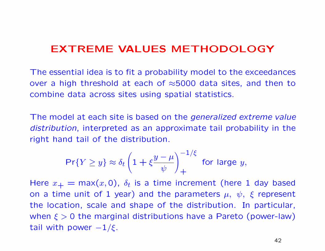
EXTREME VALUES METHODOLOGY

The essential idea is to fit a probability model to the exceedances

over a high threshold at each of ≈5000 data sites, and then to

combine data across sites using spatial statistics.

The model at each site is based on the generalized extreme value

distribution, interpreted as an approximate tail probability in the

right hand tail of the distribution.

Pr{Y ≥ y} ≈ δt(

1 + ξy − µψ

)−1/ξ

+for large y,

Here x+ = max(x,0), δt is a time increment (here 1 day based

on a time unit of 1 year) and the parameters µ, ψ, ξ represent

the location, scale and shape of the distribution. In particular,

when ξ > 0 the marginal distributions have a Pareto (power-law)

tail with power −1/ξ.

42

TEMPORAL AND SPATIAL DEPENDENCE

Here, we make two extensions of the basic methodology.

First, the parameters µ, ψ, ξ are allowed to be time-dependent

through covariates. This allows a very flexible approach to sea-

sonality, and we can also introduce linear trend terms to examine

changes in the extreme value distribution over the time period

of the study.

The second extension is spatial smoothing: after estimating the

25-year return value at each site, we smooth the results across

sites by a technique similar to kriging. We allow for spatial

nonstationarity by dividing the US into 19 overlapping boxes,

and interpolating across the boundaries.

43

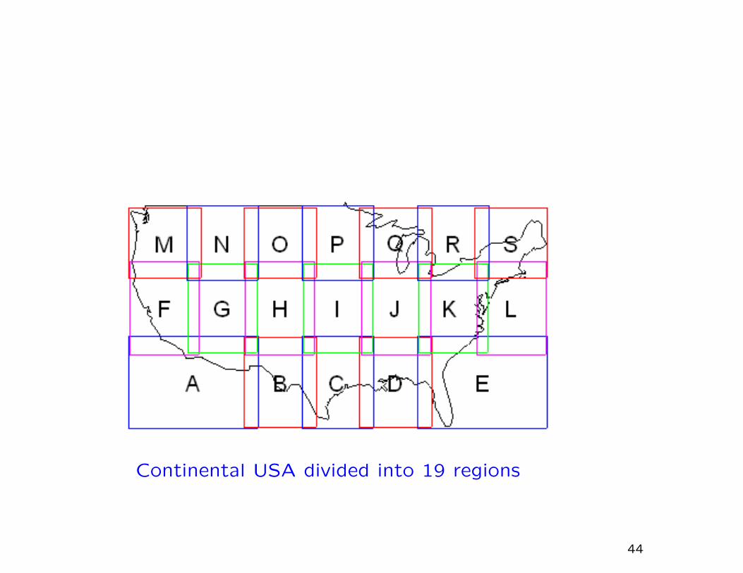
Continental USA divided into 19 regions

44

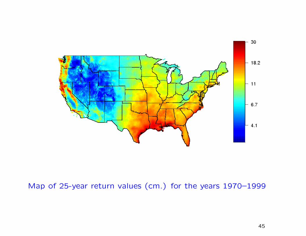
Map of 25-year return values (cm.) for the years 1970–1999

45

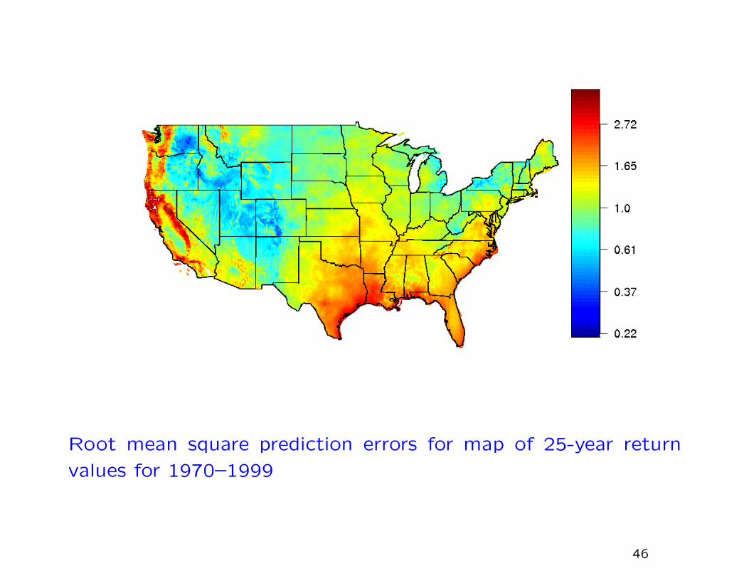
Root mean square prediction errors for map of 25-year return

values for 1970–1999

46

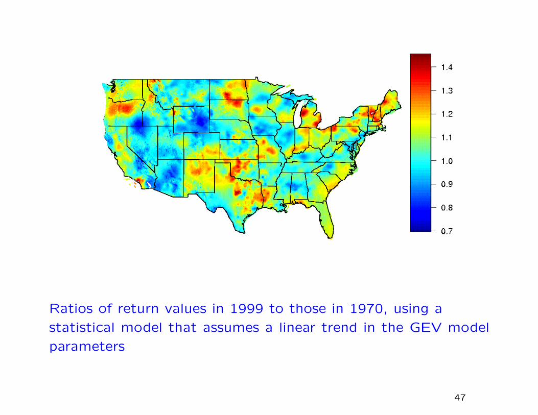
Ratios of return values in 1999 to those in 1970, using a

statistical model that assumes a linear trend in the GEV model

parameters

47

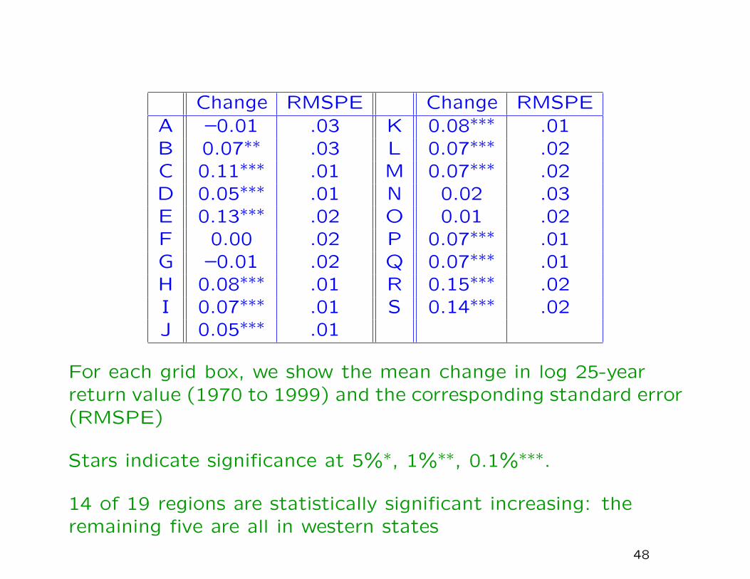
Change RMSPE Change RMSPEA –0.01 .03 K 0.08∗∗∗ .01B 0.07∗∗ .03 L 0.07∗∗∗ .02C 0.11∗∗∗ .01 M 0.07∗∗∗ .02D 0.05∗∗∗ .01 N 0.02 .03E 0.13∗∗∗ .02 O 0.01 .02F 0.00 .02 P 0.07∗∗∗ .01G –0.01 .02 Q 0.07∗∗∗ .01H 0.08∗∗∗ .01 R 0.15∗∗∗ .02I 0.07∗∗∗ .01 S 0.14∗∗∗ .02J 0.05∗∗∗ .01

For each grid box, we show the mean change in log 25-yearreturn value (1970 to 1999) and the corresponding standard error(RMSPE)

Stars indicate significance at 5%∗, 1%∗∗, 0.1%∗∗∗.

14 of 19 regions are statistically significant increasing: theremaining five are all in western states

48

We can use the same statistical methods to project future changes

by using data from climate models.

Here we use data from CCSM, the climate model run at NCAR.

49

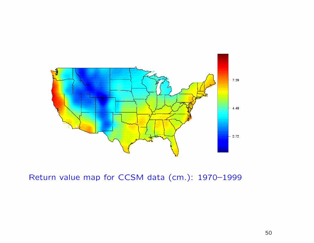
Return value map for CCSM data (cm.): 1970–1999

50

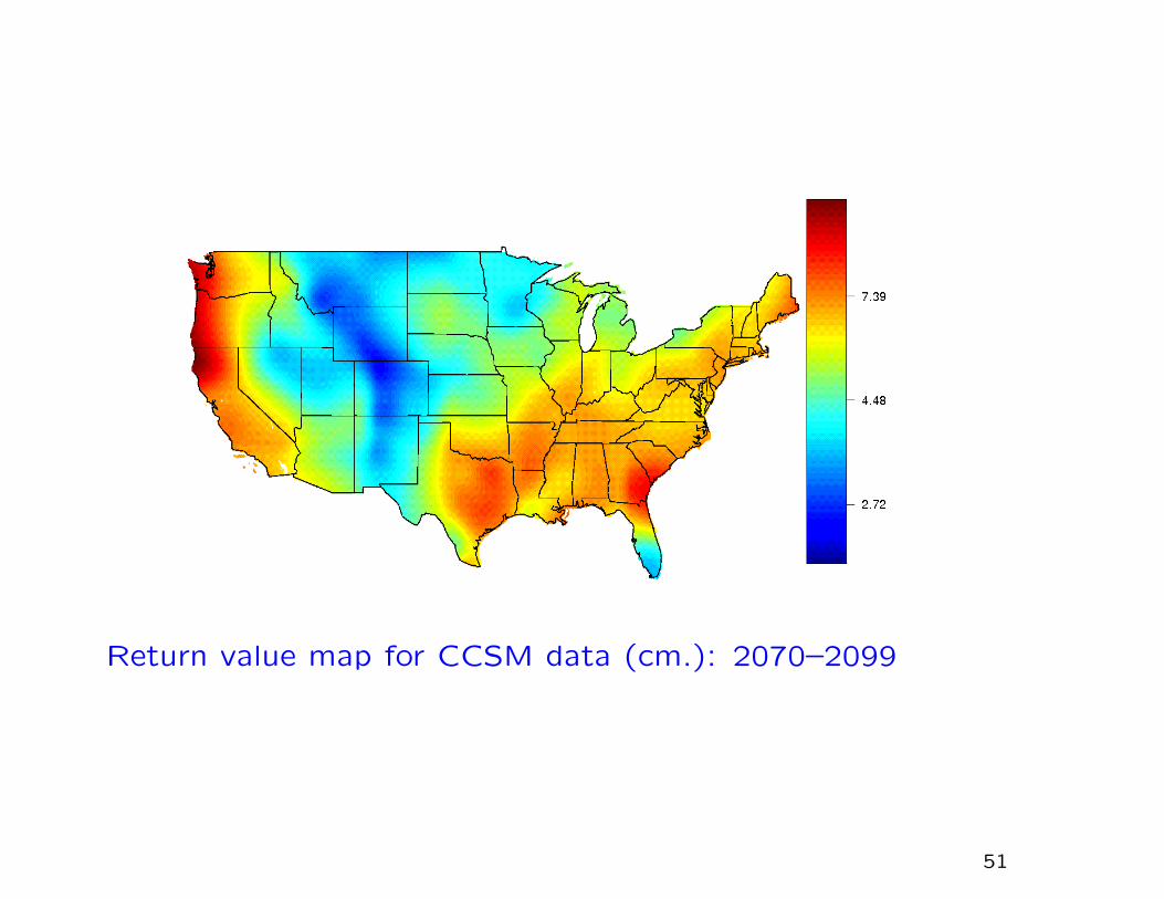
Return value map for CCSM data (cm.): 2070–2099

51

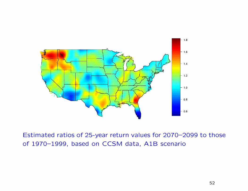
Estimated ratios of 25-year return values for 2070–2099 to those

of 1970–1999, based on CCSM data, A1B scenario

52

The climate model data show clear evidence of an increase in 25-

year return values over the next 100 years, as much as doubling

in some places.

53

A caveat...

Although the overall increase in observed precipitation

extremes is similar to that stated by other authors, the spatial

pattern is completely different. There are various possible expla-

nations, including different methods of spatial aggregation and

different treatments of seasonal effects.

Even when the same methods are applied to CCSM data over

1970–1999, the results are different.

54

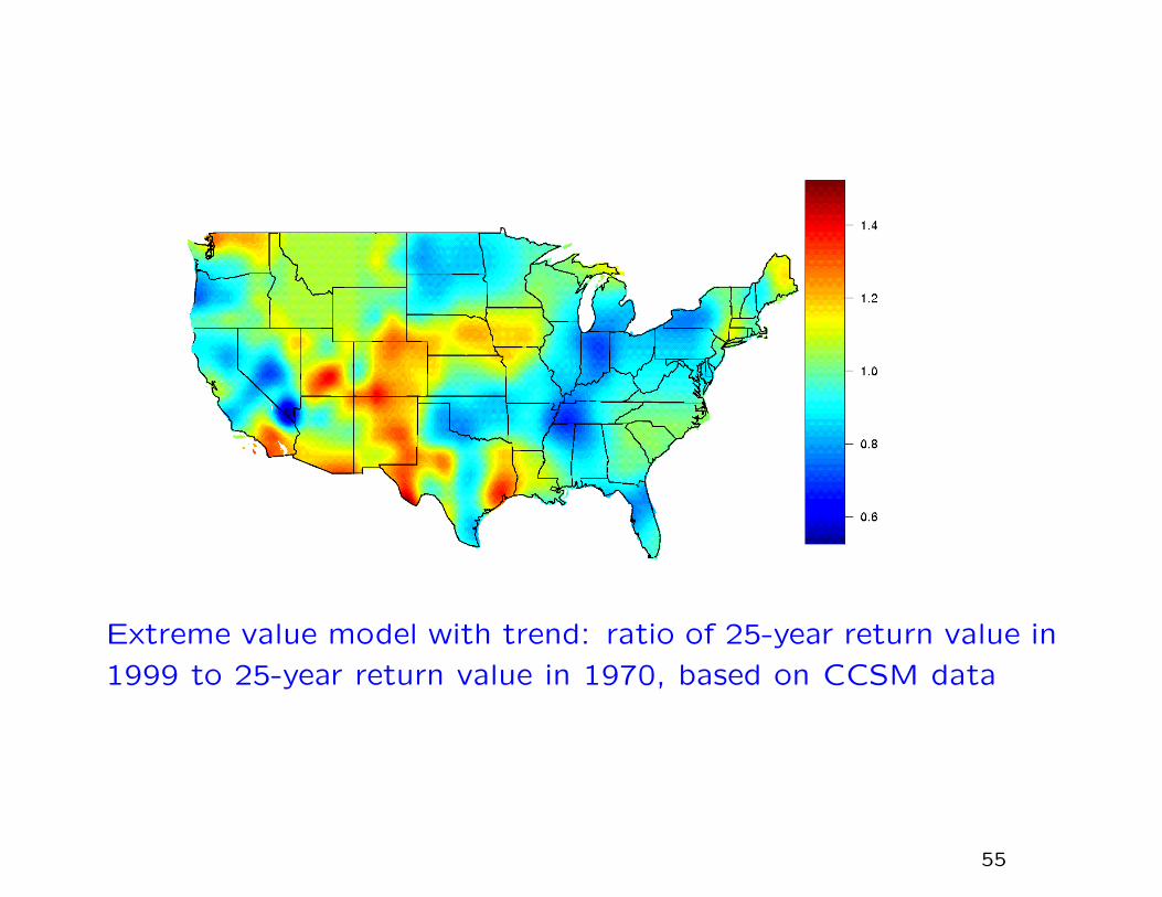
Extreme value model with trend: ratio of 25-year return value in

1999 to 25-year return value in 1970, based on CCSM data

55

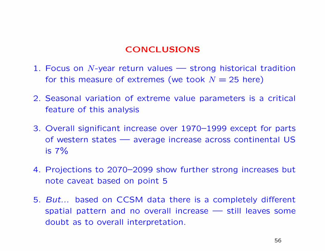
CONCLUSIONS

1. Focus on N-year return values — strong historical tradition

for this measure of extremes (we took N = 25 here)

2. Seasonal variation of extreme value parameters is a critical

feature of this analysis

3. Overall significant increase over 1970–1999 except for parts

of western states — average increase across continental US

is 7%

4. Projections to 2070–2099 show further strong increases but

note caveat based on point 5

5. But... based on CCSM data there is a completely different

spatial pattern and no overall increase — still leaves some

doubt as to overall interpretation.

56

FURTHER READING

Finkenstadt, B. and Rootzen, H. (editors) (2003), Extreme Val-

ues in Finance, Telecommunications and the Environment. Chap-

man and Hall/CRC Press, London.

(See http://www.stat.unc.edu/postscript/rs/semstatrls.pdf)

Coles, S.G. (2001), An Introduction to Statistical Modeling of

Extreme Values. Springer Verlag, New York.

57

THANK YOU FOR YOURATTENTION!

58