Journal of Applied Mechanics Vol. 1 (August 1998) JSCE

Failure Simulation of Foundation by Manifold Method

And Comparison with Experiment

マ ニフォール ド法に よる基礎破壊 の シミュ レー シ ョン と実験結果 の比較

Guoxin Zhang*, Yasuhito Sugiura** and Kozo Saito***

張 国新 ・杉浦 靖人 ・斎藤 孝三*INA Corporation . (1-44-10 Sekiguchi Bunkyoku, Tokyo)

**INA Corporation . (1-44-10 Sekiguchi Bunkyoku, Tokyo)***Member , INA Corporation. (1-44-10 Sekiguchi Bunkyoku, Tokyo)

Manifold Method (MM) is a newly developed numerical tool in analyzing bothcontinuous and discontinuous problems. By employing the concept of cover and two

sets of meshes, MM can simulate the small and large-scale deformation of materials

as well as the failure and movement of block system. In the present paper the original

MM is extended by adding the consideration of crack propagation in failure processinto the numerical procedure. The extended version of MM is then applied to simulate

the initiation and propagation of cracks in dam foundation with weak zone such as

faults and joints. The failure process and corresponding bearing capacity are predicted,

and the computed results are compared with those of the experiment. It is convincedthat the extended version of MM can reproduce the initiation of cracks and the failure

process reasonably well.

Key Words: Manifold Method, blocks, discontinuity, failure

1. Introduction

Several numerical methods are used insimulating the failure and response of structureand rock foundation with discontinuities. Thesemethods include the Finite Element Method(FEM), the Boundary Element Method (BEM),the Discrete Element Method (DEM) and theDiscontinuous Displacement Analysis (DDA).Although discontinuities in structure and rockmass can be modeled in a discrete manner withFEM and BEM by using special joint elements

(such as Goodman Element), it is difficult todescribe the discontinuities numerically, andsmall deformation restriction is usually needed.And also the number of discontinuities that canbe handled is limited. Therefore, problems ofmany discontinuities or large-scale deformationcan not be analyzed by such kind of methods.DEM and DDA can be utilized to model thebehavior of structure with many discontinuties

or block system, but the stress distributioninside the blocks can not be calculated properly,

and, therefore, the propagation of cracksthrough blocks can not be well modeled.

Manifold Method (MM) proposed by Shi in

19911) is a new numerical method. It provides a

unified framework for solving problems withboth continuous and discontinuous media. The

concept and potential application of this methodhave drawn a great attention from international

researchers in engineering fields2) 3) 4) 5) 6) 7) 8).

By employing the concept of cover and twosets of meshes, manifold Method combined the

advantages of FEM and DDA. It can not only

deal with discontinuities, contact, large scale

deformation and block movement as DDA, butalso provide the stress distribution inside each

block accurately as FEM can.

In the present paper, the original ManifoldMethod is extended to simulate the failure of

existing joints and the propagation of cracks

•\ 427

inside blocks. As examples, the failure of two

dam foundations is simulated by the extended

MM and the results are compared with those of

the experiment.

2. Basic Concepts of Manifold Method

2.1 Cover and Two Sets of MeshesThe most innovative features of Manifold

Method are the concept of cover and the use oftwo sets of meshes. Every cover covers a fixedarea, the shape and size of this area can bechosen freely according to the problem to besolved. The covers overlap each other and coverthe whole physical area. In each cover, a localfunction is defined. By means of weight function,the local functions are combined to form the

global function and define the displacement andstress in the whole region.

The two sets of meshes are physical meshesand mathematical meshes. The physical meshesdescribe the physical domain includingboundaries, joints and the interfaces betweenblocks, and define the integration area. The

physical meshes are definitely determined bythe problem to be analyzed. The mathematicalmeshes, on the other hand, are closed linesselected more or less arbitrarily by users. Theenclosed areas by the mathematical meshes arecalled mathematical covers, on which the spacefunction is built. The mathematical meshesshould be large enough to cover every point ofthe physical meshes.

The physical and mathematical meshesintersect each other and form the physicalcovers. If the physical meshes divide amathematical cover into two or more completelydisconnected domains, these domains are calledas physical covers.

All the closed areas generated by theintersection between physical meshes andmathematical meshes are defined as thecalculation elements. One calculation elementmay be covered by one or more physical covers,and its behavior is determined by these covers.

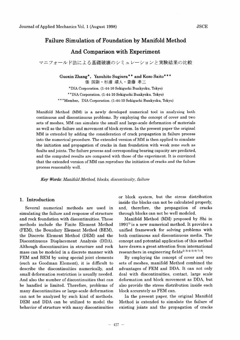
Fig. 1 gives an example of general covers ofMM in blocks with one joint. Two circles and onerectangle (thin lines) delimit threemathematical covers V1, V2 and V3 to form themathematical meshes. The physical meshes

(thick lines) divide V1 into two physical covers 11and 12, V2 into two physical covers 21 and 22,

and V3 into two physical covers 31 and 32. Eleven

calculation elements are generated by the

intersection of two sets of meshes and are

denoted in this figure as11, 1122, 112231, 122132,

etc.

Fig. 1 General covers with one joint1)

Fig. 2 FEM type covers of MM in one block

with two joints

Fig.2 gives an example of FEM type covers.

Seven hexagonal mathematical covers around

seven points 1-7 are given in this figure

referring to thin lines. The physical meshes

(thick lines, one block with two joints a-b and c-d) divide the mathematical cover around point 3

into two physical covers 31 and 32, divide themathematical cover around point 5 into two

physical covers 51 and 52. Nine physical covers(1,2,31,32,4, etc) and seven calculation elements

(124, 2452, 4527, etc) are generated.

―428―

2.2 Local Function and Global FunctionIf the local cover function ui(x,y) is defined on

physical cover Ui:

Then the global function u(x,y) on the whole

physical cover system can be defined from thelocal cover functions:

where wi(x,y) is weight function defined as:

With the finite cover concept and the

definition of local and global function, manifold

method can model a wide variety of continuous

and discontinuous materials, and FEM and

DDA can be deemed as special cases of it.

2.3 Simultaneous Equilibrium Equations

For structural analysis problem, if the local

displacement function on each physical cover is

assumed to be constant, that is, the local

displacement function on cover U, is:

then the simultaneous equilibrium equations o1f

a problem with n physical covers take the form

as:

(1)

where Kij is 2•~2 sub-matrix. Kii is defined by

the shape and material properties of physical

cover i, and Kit (i•‚j) depends on the overlapping

or contact between cover i and cover j. Fi is

the load matrix acted on cover i. Equation (1)

was derived by Shi 1) 2) according to minimum

energy theory. Matrix [K] includes the

stiffness of element, inertia matrix, stiffness of

fixed points and contact stiffness. The load

vector [F] includes initial load, point load,

inertia load and contact load etc. The details of

equation (1) can be found in Shi1) 2).

3. Modeling the Existing Joint

For an existing joint, there are two

possibilities: 1) unfailed, namely the joint can be

treated as continuous, and it can transfer both

normal and shear stresses. 2) failed, that means

the joint can only transfer normal compression

stress or shear stress if the friction angle „U is

not zero.

Modeling of the existing joint considers these

two possibilities. Fig.3 shows schematically the

treatment of the joint by adding normal and

shear springs at the joint. For the former case, if

the thickness of joint layer is idealized as zero,

there must be no relative normal displacement

between two surfaces of the joint since they

keep moving together under load. A very hard

spring p (penalty) is therefore added in the

normal direction to the joint to hold the possible

relative normal displacement between two

surfaces back to zero. In the tangent direction,

however, a small relative shear displacement is

usually permitted, especially when a soft layer

is included in the joint. This condition is

satisfied by adding a soft shear spring Ks in the

tangent direction. For the later case in which

joint failed, normal penalty and shear springs

are added at the joint when the joint is loaded

by compression and the shear stress is less than

the friction between two surfaces. If the shear

stress is larger than the friction, shear spring is

removed and only normal spring is needed. If

the joint opens, both normal and shear springs

are removed from the joint.

•\ 429•\

Fig.3 The normal and shear springs of

contact blocks

In the present paper the failure process of

existing joints is handled in the following way.

Assume that failure of existing joints follows

Mohr-Coulomb's law with three parameters.

Taking ƒÐ'y as the normal stress and ƒÑxy as the

shearing stress on a joint, the failure criterion is

defined as bellow:

tensile failure

shearing failure (2)

shearing failure

where T0represents the tension strength of joint,

Crepresents cohesion, ƒÓ is the friction angle.

4. Crack Propagation in Solid Block

In rock foundation or concrete structure,cracks occur usually from weak zone like faults,

joints and interfaces of different materials. Withthe propagation, the cracks break the mass

material and lead to the final failure. Modelingthe failure of foundation and structure must

simulate both the opening of existing joints and

the fracturing of mass materials.Manifold Method is extended to simulate

crack propagation in the present paper. When anew crack occurs or an old crack propagates the

physical meshes and the mathematical meshesthat contain this crack should be regenerated. If

no physical cover is broken by the new crack,

then only the physical meshes need to bereformed, the mathematical meshes keep

unchanged. But if the new crack breaks a

physical cover into two parts, then a newphysical cover is produced, hence both the

physical and mathematical meshes must beregenerated.

Fig. 4 is given here to illustrate the crack

propagation and corresponding regeneration ofthe physical and mathematical mesh system inthe numerical simulation. In Fig.4(a) a new

crack ab occurs. Since it does not break the

physical cover that contains it into two parts,only physical meshes need to be regenerated byadding ab into the physical meshes. The

mathematical meshes keep unchanged.

Whereas in Fig.4(b), new occurred crack be

together with the existing crack ab break the

cover that covers the area 4-5-8-10-9-6 into two

parts, therefore a new cover must be added tothe previous physical covers, and both the

physical and mathematical meshes need to beregenerated.

In simulating the failure of solid block,

formula (2) is also taken as the failure criterion.

But in the present study, it is supposed that

new cracks can only propagate along themathematical meshes.

(a) (b)

Fig.4 The relationship between new crack

and covers

5. Application Examples

The safety of an arch dam depends mainly on

the stability of the arch abutments. The

stability and bearing capacity of the dam

foundation are usually studied by experiment9.

In this section the newly extended version of

Manifold Method is applied to analyze the

stability and bearing capacity of dam foundation

and to simulate their failure process. The

numerical results are compared with the

experimental ones.

―430―

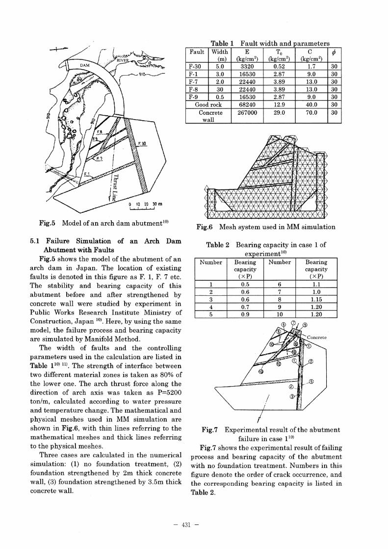
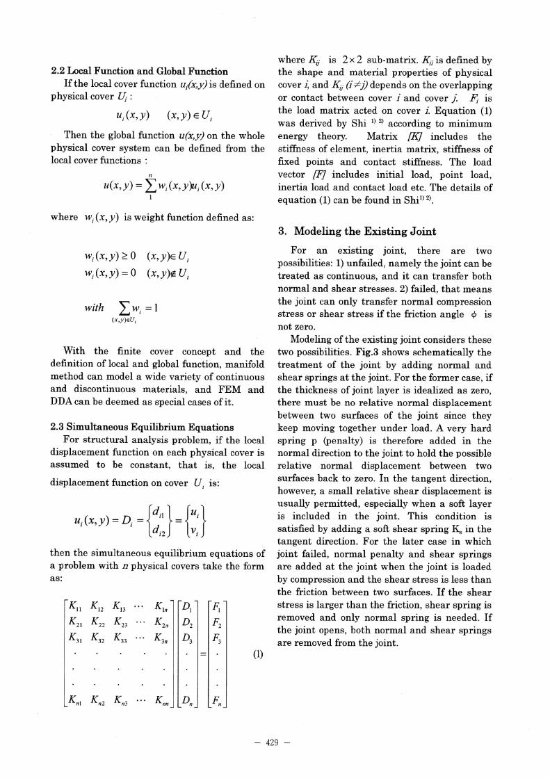
Fig.5 Model of an arch dam abutment10)

5.1 Failure Simulation of an Arch Dam

Abutment with Faults

Fig.5 shows the model of the abutment of an

arch dam in Japan. The location of existingfaults is denoted in this figure as F. 1, F. 7 etc.

The stability and bearing capacity of this

abutment before and after strengthened by

concrete wall were studied by experiment inPublic Works Research Institute Ministry ofConstruction, Japan10). Here, by using the same

model, the failure process and bearing capacity

are simulated by Manifold Method.The width of faults and the controlling

parameters used in the calculation are listed inTable 110)11). The strength of interface between

two different material zones is taken as 80% ofthe lower one. The arch thrust force along the

direction of arch axis was taken as P=5200ton/m, calculated according to water pressure

and temperature change. The mathematical and

physical meshes used in MM simulation areshown in Fig.6, with thin lines referring to themathematical meshes and thick lines referring

to the physical meshes.

Three cases are calculated in the numericalsimulation: (1) no foundation treatment, (2)

foundation strengthened by 2m thick concrete

wall, (3) foundation strengthened by 3.5m thick

concrete wall.

Table 1 Fault width and parameters

Fig.6 Mesh system used in MM simulation

Table 2 Bearing capacity in case 1 of

experiment10)

Fig.7 Experimental result of the abutment

failure in case 110)

Fig.7 shows the experimental result of failing

process and bearing capacity of the abutmentwith no foundation treatment. Numbers in this

figure denote the order of crack occurrence, and

the corresponding bearing capacity is listed in

Table 2.

―431―

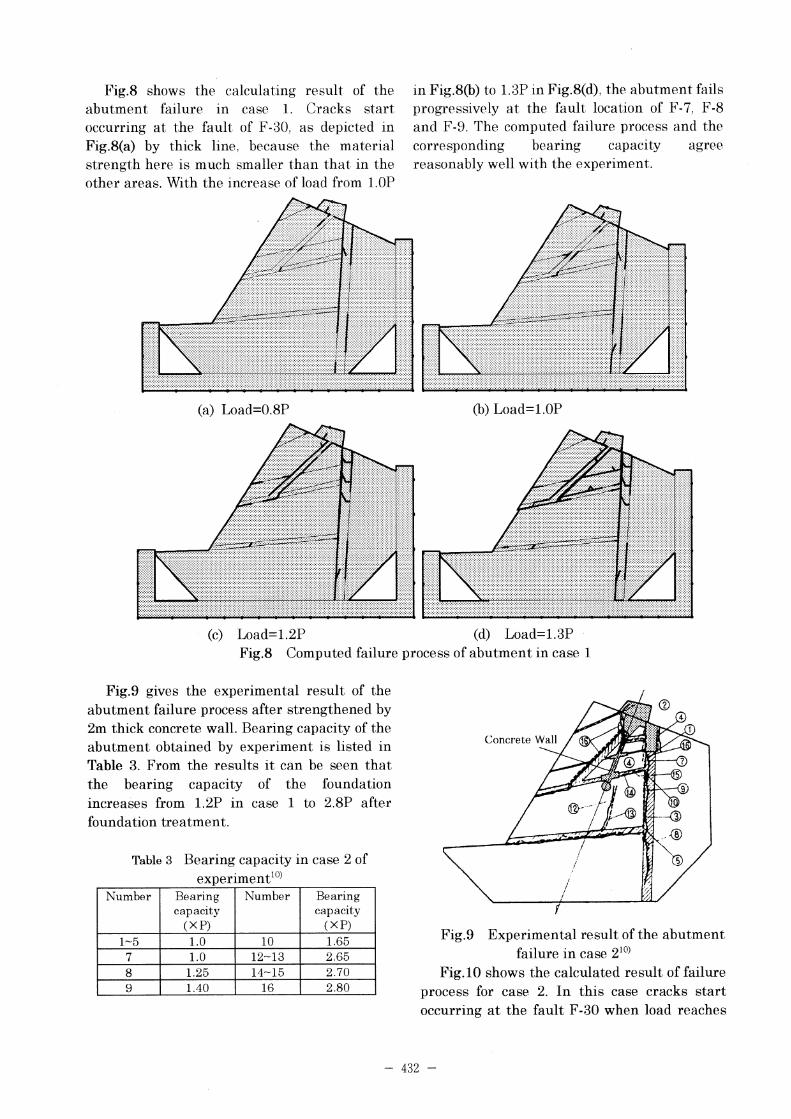
Fig.8 shows the calculating result of the

abutment failure in case 1. Cracks start

occurring at the fault of F-30, as depicted in

Fig.8(a) by thick line, because the material

strength here is much smaller than that in the

other areas. With the increase of load from 1.0P

in Fig.8(b) to 1.3P in Fig.8(d), the abutment fails

progressively at the fault location of F-7, F-8and F-9. The computed failure process and the

corresponding bearing capacity agree

reasonably well with the experiment.

(a) Load=0.8P

(c) Load=1.2P

(b) Load=1.0P

(d) Load=1.3PFig.8 Computed failure process of abutment in case 1

Fig.9 gives the experimental result of the

abutment failure process after strengthened by

2m thick concrete wall. Bearing capacity of the

abutment obtained by experiment is listed in

Table 3. From the results it can be seen that

the bearing capacity of the foundation

increases from 1.2P in case 1 to 2.8P after

foundation treatment.

Table 3 Bearing capacity in case 2 of

experiment10)

Fig.9 Experimental result of the abutment

failure in case 210)

Fig.10 shows the calculated result of failure

process for case 2. In this case cracks startoccurring at the fault F-30 when load reaches

―432―

0.6P, as shown in Fig.10(a). In Fig.10(b) when

load reaches 2.0P, almost all the area of F-30

failes, and faults at F-8 and F-9 start opening.

When load further increas to 2.6P, shown in

Fig.10(c), the concrete wall begins to fail,

leading to the failure of the foundation along

F-30 to F-1. Following the failure of foundation,

blocks lose their stability and begin to move.

Fig.10(d) shows the movement of blocks after

the foundation failure.

(a) Load=0.6P

(c) Load=2.6P

(b) Load=2.0P

(d) The Movement of BlocksFig.10 Computed failure process of the abutment in case 2

Fig.11 Experimental result after the

foundation treatment by 3.5m concrete wall10)

Experimental result of the abutment failure

for case 3 is given in Fig.11 and the

corresponding bearing capacity is listed in

Table. 4. The bearing capacity increases to 4.0P

due to the treatment of foundation by 3.5m

thick concrete wall. The simulation result for

the same case is shown in Fig.12. The

prediction of bearing capacity is slightly larger

than the experimental one. The failure process

is similar to the experiment.

Table 4 Bearing capacity in case 310)

―433―

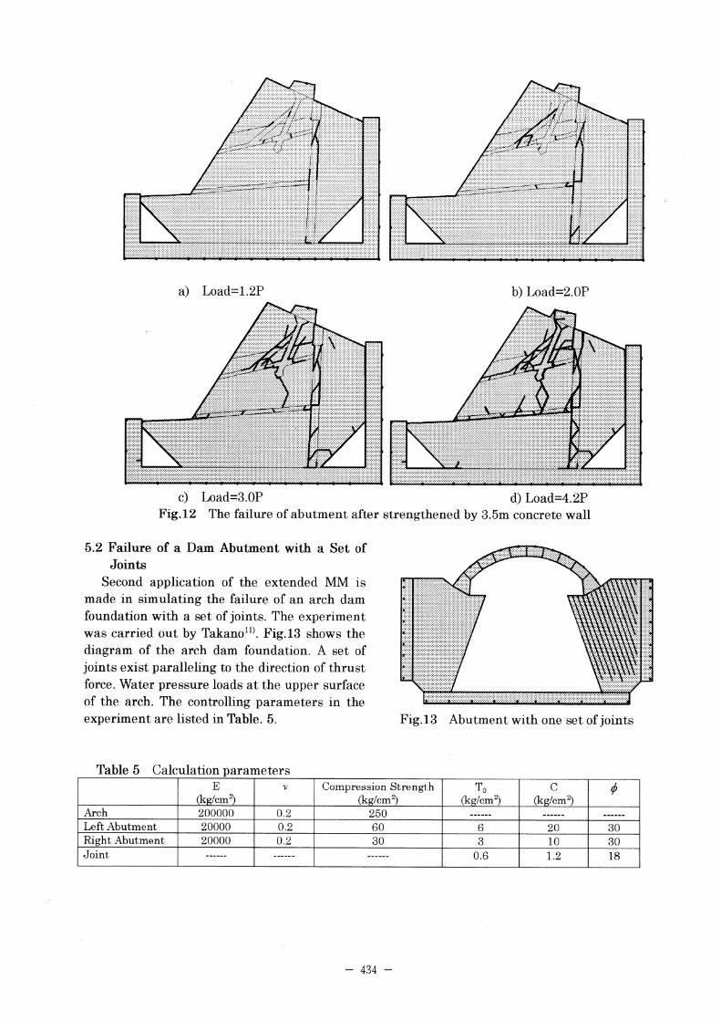
a) Load=1.2P

c) Load=3.0P

b) Load=2.0P

d) Load=4.2PFig.12 The failure of abutment after strengthened by 3.5m concrete wall

5.2 Failure of a Dam Abutment with a Set of

Joints

Second application of the extended MM ismade in simulating the failure of an arch dam

foundation with a set of joints. The experiment

was carried out by Takano11). Fig.13 shows the

diagram of the arch dam foundation. A set of

joints exist paralleling to the direction of thrustforce. Water pressure loads at the upper surface

of the arch. The controlling parameters in the

experiment are listed in Table. 5. Fig.13 Abutment with one set of joints

Table 5 Calculation parameters

―434―

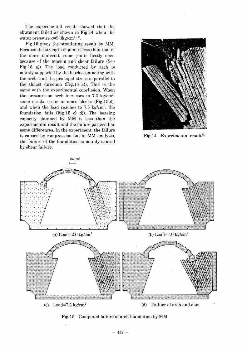
The experimental result showed that the

abutment failed as shown in Fig.14 when the

water pressure q=9.3kg/cm211).Fig.15 gives the simulating result by MM.

Because the strength of joint is less than that of

the mass material, some joints firstly open

because of the tension and shear failure (SeeFig.15 a)). The load conducted by arch is

mainly supported by the blocks contacting with

the arch, and the principal stress is parallel to

the thrust direction (Fig.15 a)). This is the

same with the experimental conclusion. When

the pressure on arch increases to 7.0kg/cm2,

some cracks occur in mass blocks (Fig.15b)),

and when the load reaches to 7.5kg/cm2, thefoundation fails (Fig.15 c)d)). The bearing

capacity obtained by MM is less than the

experimental result and the failure pattern has

some differences. In the experiment, the failuris caused by compression but in MM analysis,

the failure of the foundation is mainly caused

by shear failure.

Fig.14 Experimental result11)

(a) Load=2.0kg/cm2

(c) Load=7.5kg/cm2

(b) Load=7.0kg/cm2

(d) Failure of arch and dam

Fig.15 Computed failure of arch foundation by MM

―435―

6. Conclusion

Manifold Method is a newly developednumerical tool in analyzing continuous anddiscontinuous problems. In the present paperthe original MM was extended by adding theconsideration of crack propagation in failure

process into the numerical procedure. Theextended version of MM is capable of dealingwith the failure of structure or foundation with

joints or faults. Application examples weregiven in simulating the failure process of a damabutment with faults and a dam foundationwith joints. The prediction results of thebearing capacity and the failure process are ingood agreement with the experiments. It isconvinced that the extended version of MM canreproduce the initiation of cracks, the failureprocess and block movement reasonably well.From engineering practical point of view, thenumerical method developed in the presentstudy would be a very useful tool in simulatingthe failure process of structure withdiscontinuities.

Acknowledgments

The author would like to thank Dr. G. H. Shiand Professor Yuzo OHNISHI for suggestions.

Reference

1) Shi, G. H., Manifold Method of MaterialAnalysis. Proc. Ninth Army Conference onApplied Mathematics and Computing,Minneapolis, Minnesota, U. S. A., pp. 51-76,June 18-21, 1991.

2) Shi Genhua, Manifold Method,Discontinuous Deformation Analysis (DDA)and Simulations of Discontinuous Media,pp.52-204, TSI Press 1996.

3) Jeen-Shang Lin, Continuous andDiscontinuous Analysis Using the ManifoldMethod. Working Forum on the ManifoldMethod of Material Analysis. Jenner,California, USA, (1996). Vol. 1, pp.1-20.

4) Chiao-Tung Chang, Nonlinear LevelManifold Method, Working Forum on theManifold Method of Material Analysis.Jenner, California, USA, (1996). Vol. 1, pp.127-146.

5) Mary MacLaughlin, Manifold Application:Tunnel Roof Deflection. Working Forum on

the Manifold Method of Material Analysis.Jenner, California, USA,(1996). Vol. 1, pp.241-244.

6) Guo-Xin Zhang, Yasuhito Sugiura andHiroo Hasegawa, Crack propagation addthermal fracture analysis by ManifoldMethod, Proceedings of the SecondInternational Conference on Analysis ofDiscontinuous Deformation, July 10-12, 1997, Kyoto Japan, pp.282-297.

7) Yaw-Jeng Chiou, Crack Propagation UsingManifold Method. Proceedings of theSecond International Conference onAnalysis of Discontinuous Deformation,July 10-12, 1997,Kyoto Japan, pp.298-308.

8) Guang-Qi Chen, Yozo Ohnishi andTakahiro Ito. Development of High OrderManifold Method. Proceedings of theSecond International Conference onAnalysis of Discontinuous Deformation,July 10-12,1997,Kyoto Japan. pp.132-154.

9) R. Iida, Design Method of Concrete Dam,GIHODO Press, February 1992.

10) K. Nakamura, R. Iida and T. Tsutaya,Model Study on Foundation Rocks ofKawamata Dam, Report of The PublicWorks Research Institute Ministry ofConstruction, Vol. 120, No.78, pp. 1-11,October 1964.

11) Minoru Takano, Studies on ExperimentalMethod of Measuring Safety of Arch DamFoundation , Transactions of the JapanSociety of Civil Engineers, No. 78, pp.43-69,January 1962.

(Received April 24, 1998)

•\ 436•\