Fare Fisica con il computer

Maria Peressi (peressi@ts.infn.it)

Dipartimento di Fisica di UniTS e CNR-IOM

3 dicembre 2014 - “I LINCEI PER LA SCUOLA” - Lezioni Lincee in Fisica

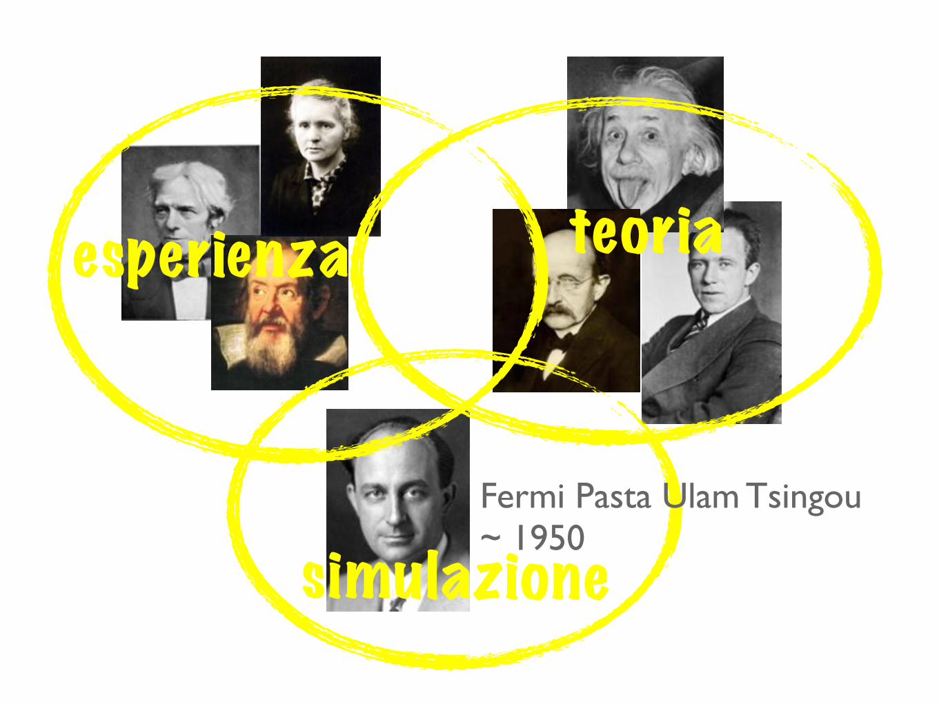
esperienza teoria

simulazioneFermi Pasta Ulam Tsingou~ 1950

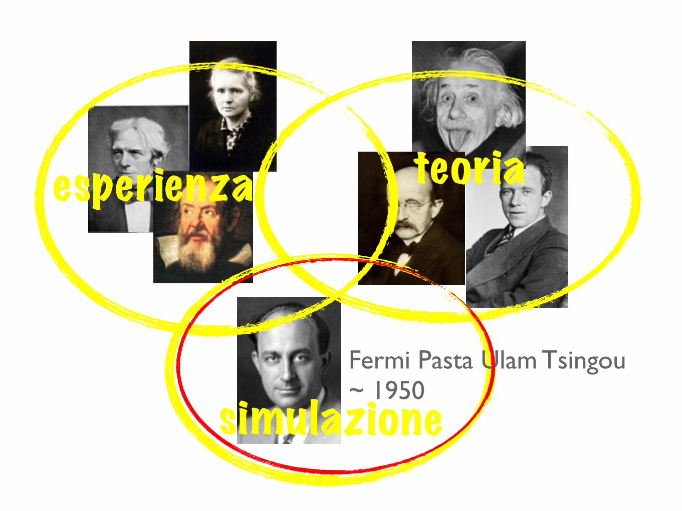
esperienza teoria

simulazioneFermi Pasta Ulam Tsingou~ 1950

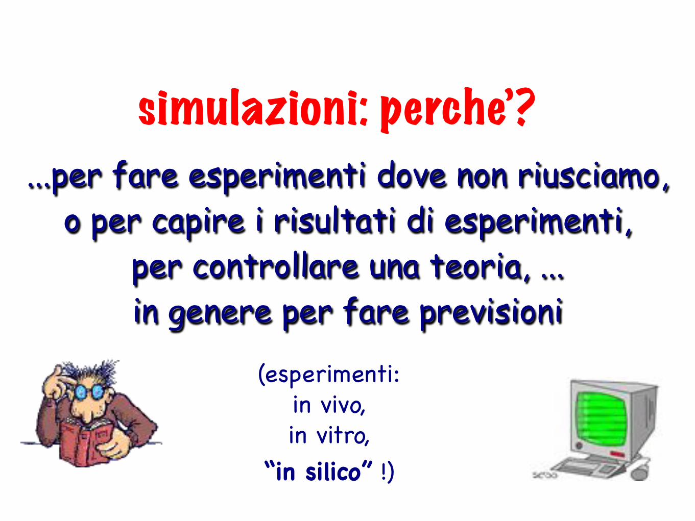
...per fare esperimenti dove non riusciamo, o per capire i risultati di esperimenti,

per controllare una teoria, ... in genere per fare previsioni

simulazioni: perche’?

(esperimenti:in vivo,in vitro,

“in silico” !)

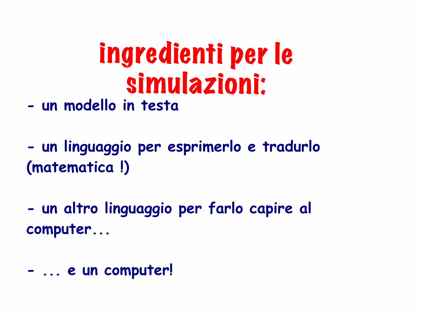
ingredienti per le simulazioni:

- un modello in testa

- un linguaggio per esprimerlo e tradurlo (matematica !)

- un altro linguaggio per farlo capire al computer...

- ... e un computer!

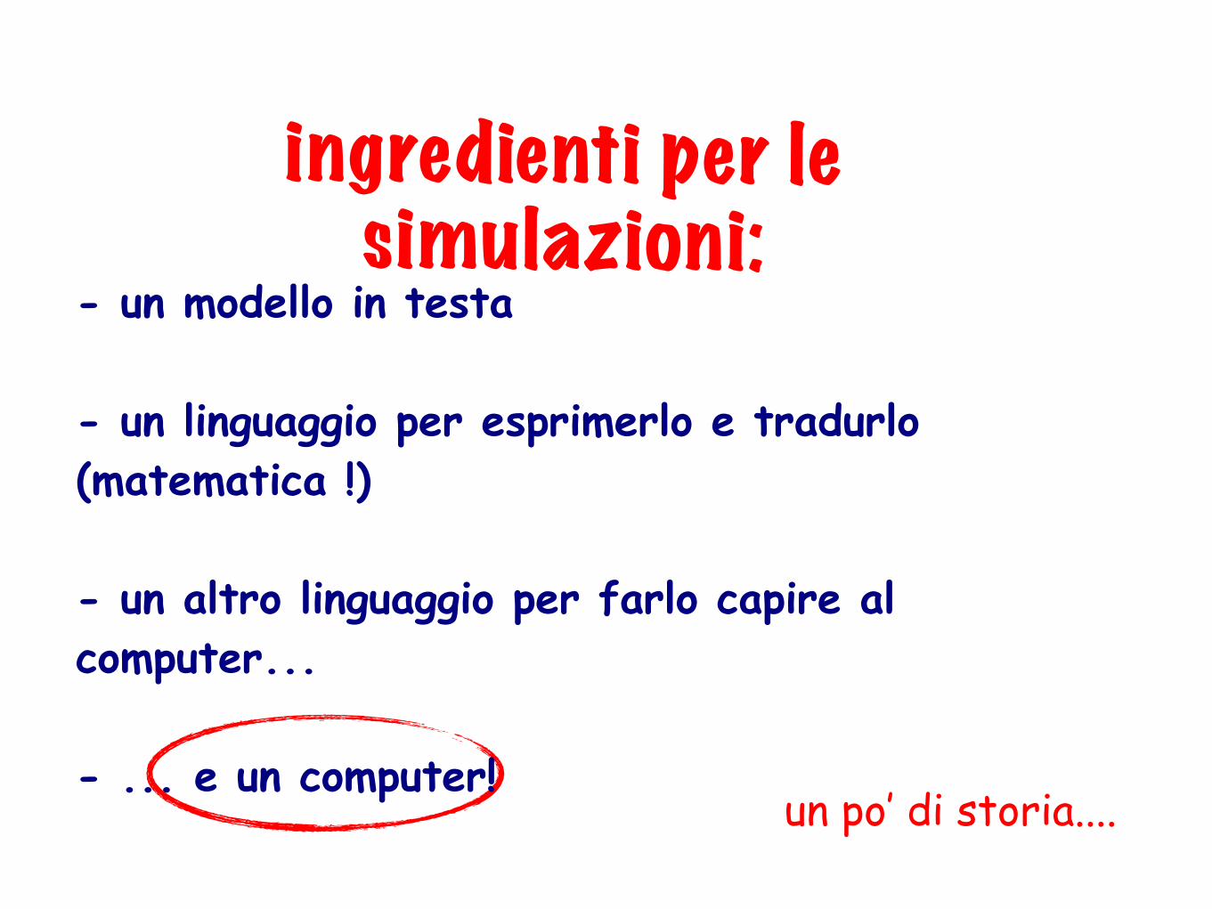
ingredienti per le simulazioni:

un po’ di storia....

- un modello in testa

- un linguaggio per esprimerlo e tradurlo (matematica !)

- un altro linguaggio per farlo capire al computer...

- ... e un computer!

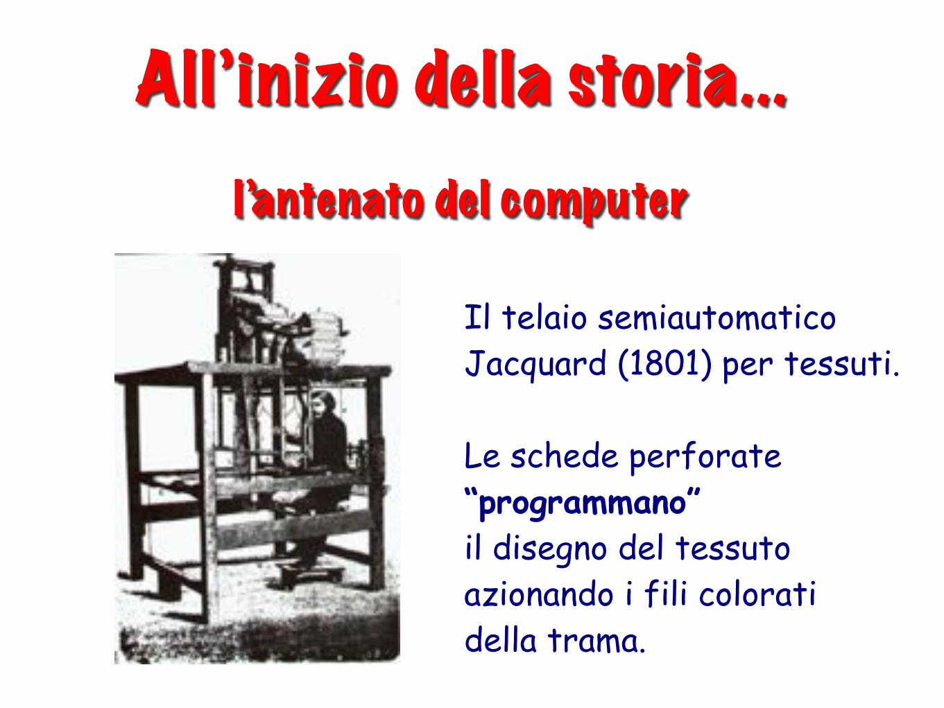
All’inizio della storia...l’antenato del computer

Il telaio semiautomatico Jacquard (1801) per tessuti. Le schede perforate “programmano” il disegno del tessuto azionando i fili colorati della trama.

All’inizio della storia...(inizio XIX sec)

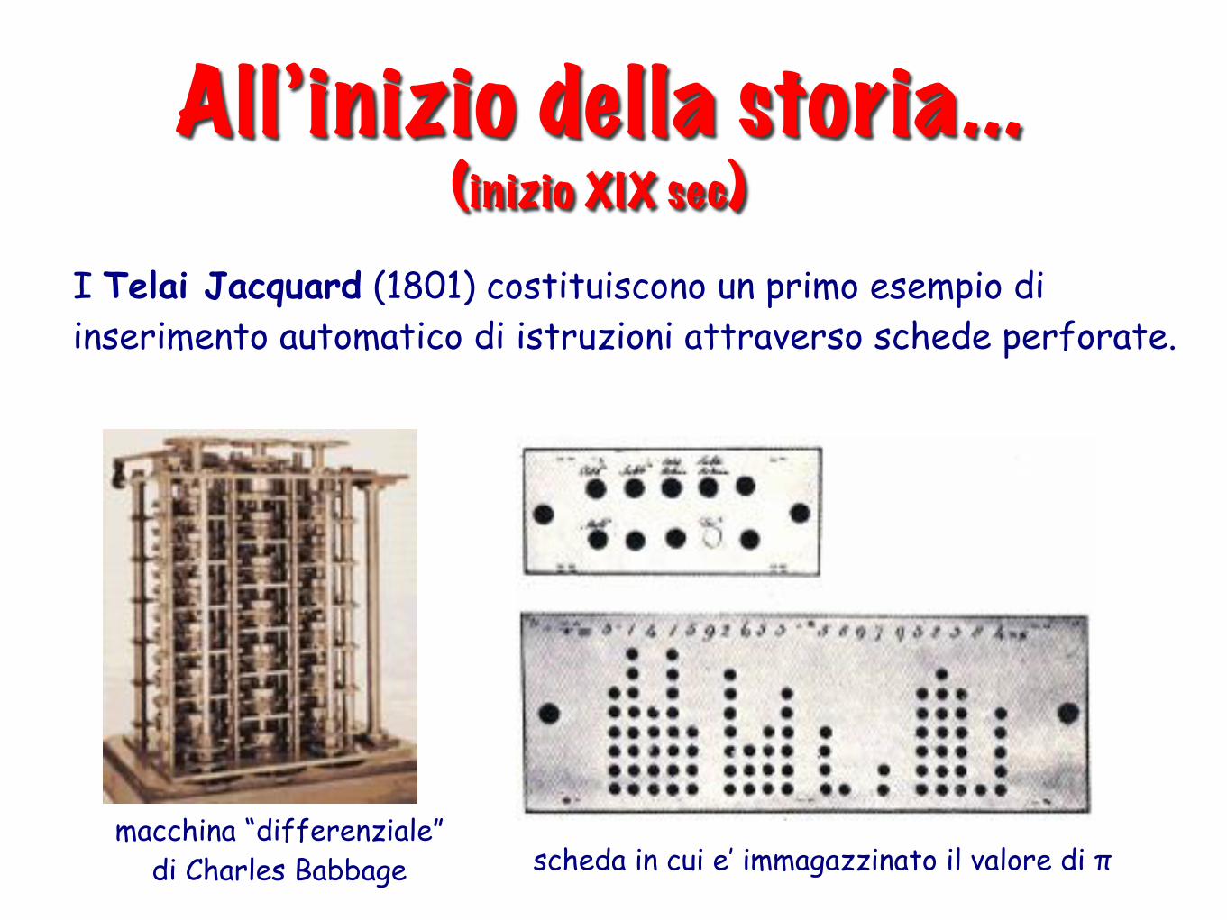
I Telai Jacquard (1801) costituiscono un primo esempio di inserimento automatico di istruzioni attraverso schede perforate.

scheda in cui e’ immagazzinato il valore di πmacchina “differenziale”

di Charles Babbage

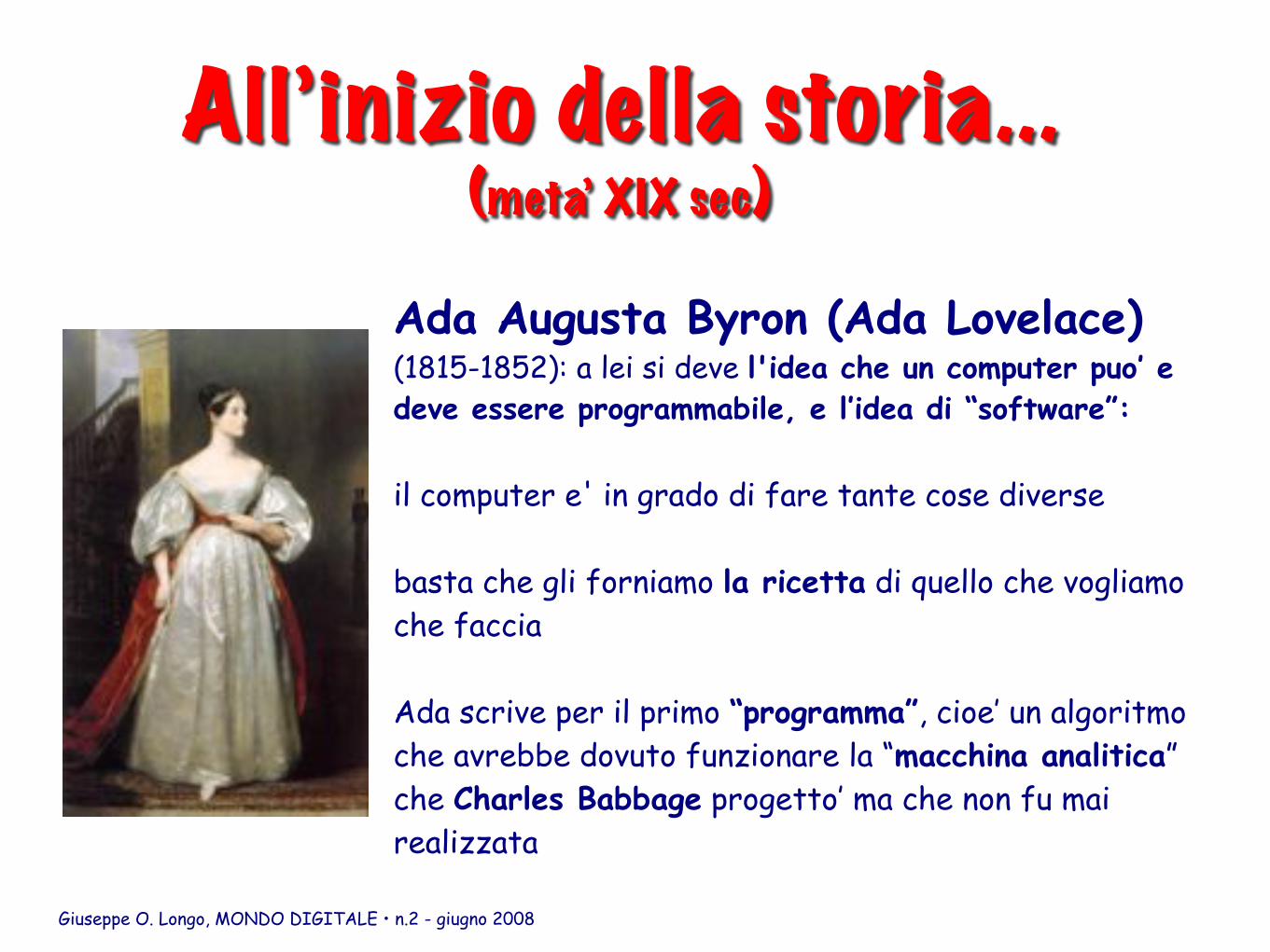
Ada Augusta Byron (Ada Lovelace) (1815-1852): a lei si deve l'idea che un computer puo’ e deve essere programmabile, e l’idea di “software”:

il computer e' in grado di fare tante cose diverse

basta che gli forniamo la ricetta di quello che vogliamo che faccia

Ada scrive per il primo “programma”, cioe’ un algoritmo che avrebbe dovuto funzionare la “macchina analitica” che Charles Babbage progetto’ ma che non fu mai realizzata

All’inizio della storia...(meta’ XIX sec)

Giuseppe O. Longo, MONDO DIGITALE • n.2 - giugno 2008

La scala enorme degli investimenti possibili per motivi bellici porta ad una generazione di “dinosauri del calcolo”:

Colossus, sviluppato in Inghilterra intorno al 1943, sotto la guida di Alan Turing. Utilizzato per la decrittazione dei messaggi cifrati tedeschi.Mark1, sviluppato negli Stati Uniti nel 1944. 800 Km di cavi e qualchescarafaggio (!?!)Eniac (1946). Il primo sistema “tutto elettronico”.

I dinosauri

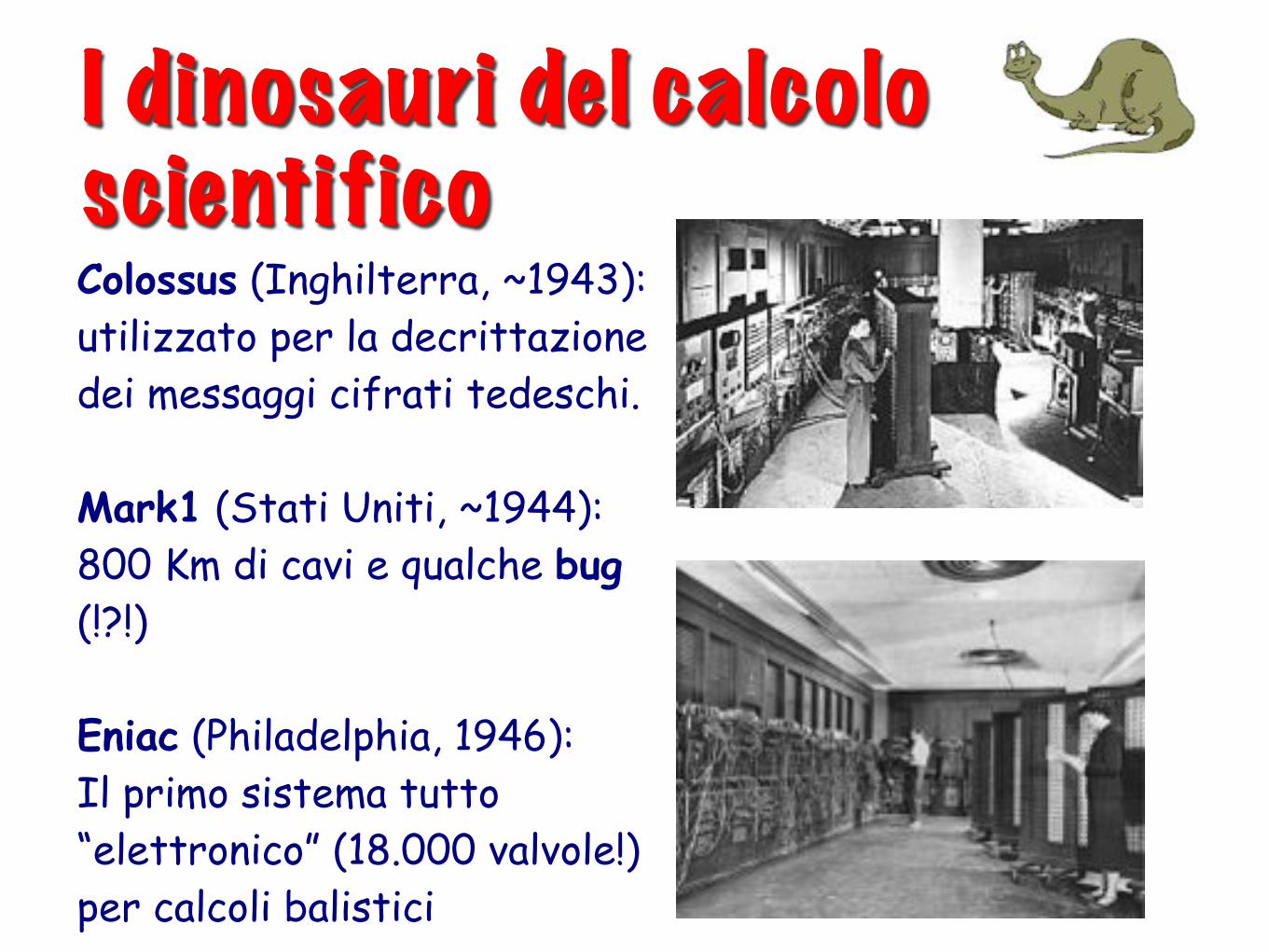
I dinosauri del calcolo scientificoColossus (Inghilterra, ~1943): utilizzato per la decrittazione dei messaggi cifrati tedeschi.

Mark1 (Stati Uniti, ~1944): 800 Km di cavi e qualche bug (!?!)

Eniac (Philadelphia, 1946):Il primo sistema tutto “elettronico” (18.000 valvole!) per calcoli balistici

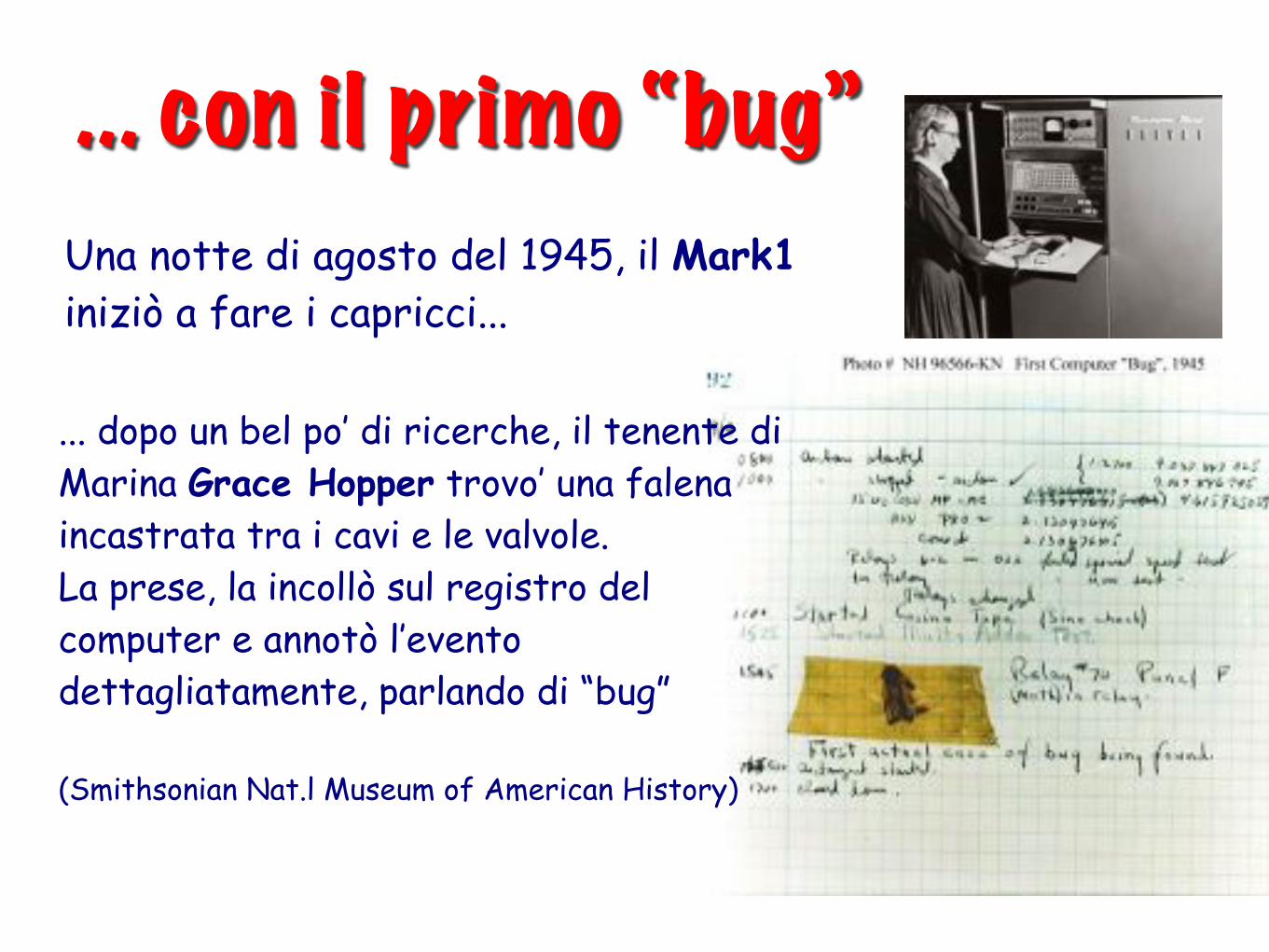
Una notte di agosto del 1945, il Mark1 iniziò a fare i capricci...

... con il primo “bug”

... dopo un bel po’ di ricerche, il tenente di Marina Grace Hopper trovo’ una falena incastrata tra i cavi e le valvole.La prese, la incollò sul registro del computer e annotò l’evento dettagliatamente, parlando di “bug”

(Smithsonian Nat.l Museum of American History)

#!⌃�⇡◆⌥⌅���⇣�⇠⌥!�⇥⌃�⇧⌫⇣���⇥ ⌃◆�⌫⇣��◆�!�"⇢⇣�"⇢⌘�

⇤⌃%*⇠⇡�⇣⌃#�'⇤!↵⌃⌥⇤�⌃⇤#⇠⌃⌥⇠�%⇤⇣�⌃#↵)↵!⇤⌃◆⇣⇠✏�#⌃⇠�⌃!↵#⇣#⇡%⇤�⌥↵⌃⇠!⌃⇤⌃�↵*⌃⌦⇣⇠⌦↵#⌧⌃⌃(✏⇣#⌃⇤⇠*#⌃⇤%⌃↵⇤#%⌃+""⌃⌥⇠��⇠�↵�%#�↵!⌃⇣�↵⇤!⌃⇣�⌥✏⌃⇠!⌃⇤⌃�'⇤!%↵!⌃�⇣⇣⇠�⌃�↵!⌃#�'⇤!↵⌃⇣�⌥✏⌧⌃(✏'#⌫-+⌫"""⌃⌥⇠��⇠�↵�%#⌃�↵↵⌦⌃⇠⌥⌥'�/⌃⇠�/⌃ ⇤⇧⇠'%⌃⇠�↵⇡�⇠'!%✏⌃ ⇤#�'⇤!↵⌃⇣�⌥✏⌧

��⌃%✏↵⌃#⇣⇣⌥⇠�⌃*⇤�↵!⌃⌥'!!↵�%/⌃'#↵⌦⌫⌃'#'⇤/⌃⇤�⌃⇣�⌥✏⌃⇠!�⇠!↵⌃⇣�⌃⌦⇣⇤�↵%↵!⌫⌃%✏↵!↵⌃⇣#⌃⇤��↵⌃!⇠⇠�⌃�⇠!⌃#'⌥✏⌃⇤⌃#%!'⌥%'!↵⌃⇣�%✏↵⌃⌥⇠��⇠�↵�%#⌃⌥⇤�⌃⇧↵⌃⌥⇠#↵/⌃�⇤⌥◆↵⌦⌃*⇣%✏⌃�⇠⌃#�⇤⌥↵⌃*⇤#%↵⌦�⇠!⌃⇣�%↵!⌥⇠��↵⌥%⇣⇠�⌃�⇤%%↵!�#⌧⌃⌃(✏⇣#⌃⇣#⌃!↵⇤⇣#%⇣⌥⌫⌃#⇣�⌥↵⌃↵��⇠!%#⌃%⇠⇤⌥✏⇣↵)↵⌃⇤⌃↵)↵⌃⇠�⌃⌥⇠��↵,⇣%/⌃⇤⇧⇠)↵⌃%✏↵⌃�!↵#↵�%/⌃⇤)⇤⇣⇤⇧↵⇣�%↵�!⇤%↵⌦⌃ ⌥⇣!⌥'⇣%#⌃ ⇤!↵⌃ ⇤!↵⇤⌦/⌃'�⌦↵!*⇤/⌃'#⇣��⌃�'%⇣⇤/↵!�↵%⇤⇣0⇤%⇣⇠�⌃�⇤%%↵!�#⌃#↵�⇤!⇤%↵⌦⌃⇧/⌃⌦⇣↵↵⌥%!⇣⌥⌃�⇣�#⌧⌃⌃&'⌥✏⌃⇤⌦↵�#⇣%/⌃⇠�⌃⌥⇠��⇠�↵�%#⌃⌥⇤�⌃⇧↵⌃⇤⌥✏⇣↵)↵⌦⌃⇧/⌃�!↵#↵�%⌃⇠�%⇣⌥⇤%↵⌥✏�⇣�'↵#⌃⇤�⌦⌃⌦⇠↵#⌃�⇠%⌃!↵�'⇣!↵⌃%✏↵⌃�⇠!↵⌃↵,⇠%⇣⌥⌃%↵⌥✏�⇣�'↵#⌫#'⌥✏⌃⇤#⌃↵↵⌥%!⇠�⌃⇧↵⇤�⌃⇠�↵!⇤%⇣⇠�#⌫⌃*✏⇣⌥✏⌃⇤!↵⌃⇧↵⇣��⌃#%'⌦⇣↵⌦⌃%⇠�⇤◆↵⌃↵)↵�⌃#�⇤↵!⌃#%!'⌥%'!↵#⌧

�⌅�◆⌃���⌅✏�⇡✓⌃� �⌃!⇤(✏↵!↵⌃⇣#⌃�⇠⌃�'�⌦⇤�↵�%⇤⌃⇠⇧#%⇤⌥↵⌃%⇠⌃⇤⌥✏⇣↵)⇣��⌃⌦↵)⇣⌥↵

/⇣↵⌦#⌃⇠�⌃$""�⌧⌃⌃⌅%⌃�!↵#↵�%⌫⌃�⇤⌥◆⇤�⇣��⌃⌥⇠#%#⌃#⇠⌃�⇤!⌃↵,⌥↵↵⌦%✏↵⌃⌥⇠#%⌃⇠�⌃%✏↵⌃#↵�⇣⌥⇠�⌦'⌥%⇠!⌃#%!'⌥%'!↵⌃⇣%#↵�⌃%✏⇤%⌃%✏↵!↵⌃⇣#⌃�⇠⇣�⌥↵�%⇣)↵⌃%⇠⌃⇣��!⇠)↵⌃/⇣↵⌦#⌫⌃⇧'%⌃%✏↵/⌃⌥⇤�⌃⇧↵⌃!⇤⇣#↵⌦⌃⇤#⌃✏⇣�✏⌃⇤#

⇣#⌃↵⌥⇠�⇠�⇣⌥⇤/⌃✓'#%⇣�⇣↵⌦⌧⌃⌃⇢⇠⌃⇧⇤!!⇣↵!⌃↵,⇣#%#⌃⌥⇠��⇤!⇤⇧↵⌃%⇠%✏↵⌃%✏↵!�⇠⌦/�⇤�⇣⌥⌃↵�'⇣⇣⇧!⇣'�⌃⌥⇠�#⇣⌦↵!⇤%⇣⇠�#⌃%✏⇤%⌃⇠�%↵�⌃⌃⇣�⇣%/⇣↵⌦#⌃⇣�⌃⌥✏↵�⇣⌥⇤⌃!↵⇤⌥%⇣⇠�#�⌃⇣%⌃⇣#⌃�⇠%⌃↵)↵�⌃�↵⌥↵##⇤!/⌃%⇠⌃⌦⇠⇤�/⌃�'�⌦⇤�↵�%⇤⌃!↵#↵⇤!⌥✏⌃⇠!⌃ %⇠⌃!↵�⇤⌥↵⌃�!↵#↵�%⌃�!⇠⌥↵##↵#⌧��/⌃%✏↵⌃↵��⇣�↵↵!⇣��⌃↵��⇠!%⌃⇣#⌃�↵↵⌦↵⌦⌧

⌘�⌃%✏↵⌃↵⇤!/⌃⌦⇤/#⌃⇠�⌃⇣�%↵�!⇤%↵⌦⌃⌥⇣!⌥'⇣%!/⌫⌃*✏↵�⌃/⇣↵⌦#⌃*↵!↵↵,%!↵�↵/⌃⇠*⌫⌃%✏↵!↵⌃*⇤#⌃#'⌥✏⌃⇣�⌥↵�%⇣)↵⌧⌃⌃(⇠⌦⇤/⌃⇠!⌦⇣�⇤!/⌃⇣�⇡%↵�!⇤%↵⌦⌃⌥⇣!⌥'⇣%#⌃⇤!↵⌃�⇤⌦↵⌃*⇣%✏⌃/⇣↵⌦#⌃⌥⇠��⇤!⇤⇧↵⌃*⇣%✏⌃%✏⇠#↵⇠⇧%⇤⇣�↵⌦⌃�⇠!⌃⇣�⌦⇣)⇣⌦'⇤⌃#↵�⇣⌥⇠�⌦'⌥%⇠!⌃⌦↵)⇣⌥↵#⌧⌃⌃(✏↵⌃#⇤�↵�⇤%%↵!�⌃*⇣⌃�⇤◆↵⌃⇤!�↵!⌃⇤!!⇤/#⌃↵⌥⇠�⇠�⇣⌥⇤⌫⌃⇣�⌃⇠%✏↵!⌃⌥⇠�#⇣⌦⇡↵!⇤%⇣⇠�#⌃�⇤◆↵⌃#'⌥✏⌃⇤!!⇤/#⌃⌦↵#⇣!⇤⇧↵⌧

⌦⌃�⇡��◆⌥ !⌃⇥.⇣⌃⇣%⌃⇧↵⌃�⇠##⇣⇧↵⌃%⇠⌃!↵�⇠)↵⌃%✏↵⌃✏↵⇤%⌃�↵�↵!⇤%↵⌦⌃⇧/⌃%↵�#

⇠�⌃%✏⇠'#⇤�⌦#⌃⇠�⌃⌥⇠��⇠�↵�%#⌃⇣�⌃⇤⌃#⇣��↵⌃#⇣⇣⌥⇠�⌃⌥✏⇣�⇥⌘�⌃*↵⌃⌥⇠'⌦⌃#✏!⇣�◆⌃%✏↵⌃)⇠'�↵⌃⇠�⌃⇤⌃#%⇤�⌦⇤!⌦⌃✏⇣�✏⇡#�↵↵⌦

⌦⇣�⇣%⇤⌃⌥⇠��'%↵!⌃%⇠⌃%✏⇤%⌃!↵�'⇣!↵⌦⌃�⇠!⌃%✏↵⌃⌥⇠��⇠�↵�%#⌃%✏↵�⇡#↵)↵#⌫⌃*↵⌃*⇠'⌦⌃↵,�↵⌥%⌃⇣%⌃%⇠⌃�⇠*⌃⇧!⇣�✏%/⌃*⇣%✏⌃�!↵#↵�%⌃�⇠*↵!⌦⇣##⇣�⇤%⇣⇠�⌧⌃ ⌃�'%⌃ ⇣%⌃*⇠� %⌃✏⇤��↵�⌃*⇣%✏⌃ ⇣�%↵�!⇤%↵⌦⌃⌥⇣!⌥'⇣%#⌧&⇣�⌥↵⌃⇣�%↵�!⇤%↵⌦⌃↵↵⌥%!⇠�⇣⌥⌃#%!'⌥%'!↵#⌃⇤!↵⌃%*⇠⇡⌦⇣�↵�#⇣⇠�⇤⌫%✏↵/⌃✏⇤)↵⌃⇤⌃#'!�⇤⌥↵⌃⇤)⇤⇣⇤⇧↵⌃�⇠!⌃⌥⇠⇠⇣��⌃⌥⇠#↵⌃%⇠⌃↵⇤⌥✏⌃⌥↵�%↵!⇠�⌃✏↵⇤%⌃�↵�↵!⇤%⇣⇠�⌧⌃⌃⌘�⌃⇤⌦⌦⇣%⇣⇠�⌫⌃�⇠*↵!⌃⇣#⌃�↵↵⌦↵⌦⌃�!⇣�⇤!⇣/⌃%⇠⌦!⇣)↵⌃%✏↵⌃)⇤!⇣⇠'#⌃⇣�↵#⌃⇤�⌦⌃⌥⇤�⇤⌥⇣%⇤�⌥↵#⌃⇤##⇠⌥⇣⇤%↵⌦⌃*⇣%✏⌃%✏↵#/#%↵�⌧⌃⌃⌅#⌃⇠��⌃⇤#⌃⇤⌃�'�⌥%⇣⇠�⌃⇣#⌃⌥⇠��⇣�↵⌦⌃%⇠⌃⇤⌃#�⇤⌃⇤!↵⇤⌃⇠�⇤⌃*⇤�↵!⌫⌃%✏↵⌃⇤�⇠'�%⌃⇠�⌃⌥⇤�⇤⌥⇣%⇤�⌥↵⌃*✏⇣⌥✏⌃�'#%⌃⇧↵⌃⌦!⇣)↵�⌃⇣#⌦⇣#%⇣�⌥%/⌃⇣�⇣%↵⌦⌧⌃⌃⌘�⌃�⇤⌥%⌫⌃#✏!⇣�◆⇣��⌃⌦⇣�↵�#⇣⇠�#⌃⇠�⌃⇤�⌃⇣�%↵⇡�!⇤%↵⌦⌃#%!'⌥%'!↵⌃�⇤◆↵#⌃⇣%⌃�⇠##⇣⇧↵⌃%⇠⌃⇠�↵!⇤%↵⌃%✏↵⌃#%!'⌥%'!↵⌃⇤%✏⇣�✏↵!⌃#�↵↵⌦⌃�⇠!⌃%✏↵⌃#⇤�↵⌃�⇠*↵!⌃�↵!⌃'�⇣%⌃⇤!↵⇤⌧

�� �⌥↵�◆⌃�⌧⌥⌅�⌅✏ ↵⇤!/⌫⌃*↵⌃*⇣⌃ ⇧↵⌃ ⇤⇧↵⌃ %⇠⌃ ⇧'⇣⌦⌃ #'⌥✏⌃ ⌥⇠��⇠�↵�%⇡

⌥!⇤��↵⌦⌃↵�'⇣��↵�%⌧⌃⌃⇢↵,%⌫⌃*↵⌃⇤#◆⌃'�⌦↵!⌃*✏⇤%⌃⌥⇣!⌥'�#%⇤�⌥↵#*↵⌃#✏⇠'⌦⌃⌦⇠⌃⇣%⌧⌃⌃(✏↵⌃%⇠%⇤⌃⌥⇠#%⌃⇠�⌃�⇤◆⇣��⌃⇤⌃�⇤!%⇣⌥'⇤!⌃#/#%↵��'�⌥%⇣⇠�⌃�'#%⌃⇧↵⌃�⇣�⇣�⇣0↵⌦⌧⌃⌃(⇠⌃⌦⇠⌃#⇠⌫⌃*↵⌃⌥⇠'⌦⌃⇤�⇠!%⇣0↵%✏↵⌃↵��⇣�↵↵!⇣��⌃⇠)↵!⌃#↵)↵!⇤⌃⇣⌦↵�%⇣⌥⇤⌃⇣%↵�#⌫⌃⇠!⌃↵)⇠)↵⌃�↵,⇡⇣⇧↵⌃%↵⌥✏�⇣�'↵#⌃�⇠!⌃%✏↵⌃↵��⇣�↵↵!⇣��⌃⇠�⌃⇤!�↵⌃�'�⌥%⇣⇠�#⌃#⇠⌃%✏⇤%�⇠⌃⌦⇣#�!⇠�⇠!%⇣⇠�⇤%↵⌃↵,�↵�#↵⌃�↵↵⌦⌃⇧↵⌃⇧⇠!�↵⌃⇧/⌃⇤⌃�⇤!%⇣⌥'⇤!⇤!!⇤/⌧⌃⌃�↵!✏⇤�#⌃�↵*/⌃⌦↵)⇣#↵⌦⌃⌦↵#⇣��⌃⇤'%⇠�⇤%⇣⇠�⌃�!⇠⌥↵⌦'!↵#⌥⇠'⌦⌃%!⇤�#⇤%↵⌃�!⇠�⌃⇠�⇣⌥⌃⌦⇣⇤�!⇤�⌃%⇠⌃%↵⌥✏�⇠⇠�⇣⌥⇤⌃!↵⇤⇣0⇤⇡%⇣⇠�⌃*⇣%✏⇠'%⌃⇤�/⌃#�↵⌥⇣⇤⌃↵��⇣�↵↵!⇣��⌧

⌘%⌃�⇤/⌃�!⇠)↵⌃%⇠⌃⇧↵⌃�⇠!↵⌃↵⌥⇠�⇠�⇣⌥⇤⌃%⇠⌃⇧'⇣⌦⌃⇤!�↵

Una previsione...

di 50 anni fa!“Cramming more components into integrated circuits” by Gordon E. Moore

http://download.intel.com/research/silicon/Gordon_Moore_1965_article.pdf

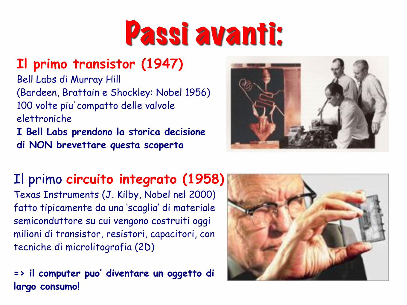
Passi avanti:Il primo transistor (1947) Bell Labs di Murray Hill (Bardeen, Brattain e Shockley: Nobel 1956)100 volte piu'compatto delle valvole elettronicheI Bell Labs prendono la storica decisione di NON brevettare questa scoperta

Il primo circuito integrato (1958)Texas Instruments (J. Kilby, Nobel nel 2000)fatto tipicamente da una ‘scaglia’ di materiale semiconduttore su cui vengono costruiti oggi milioni di transistor, resistori, capacitori, con tecniche di microlitografia (2D)

=> il computer puo’ diventare un oggetto di largo consumo!

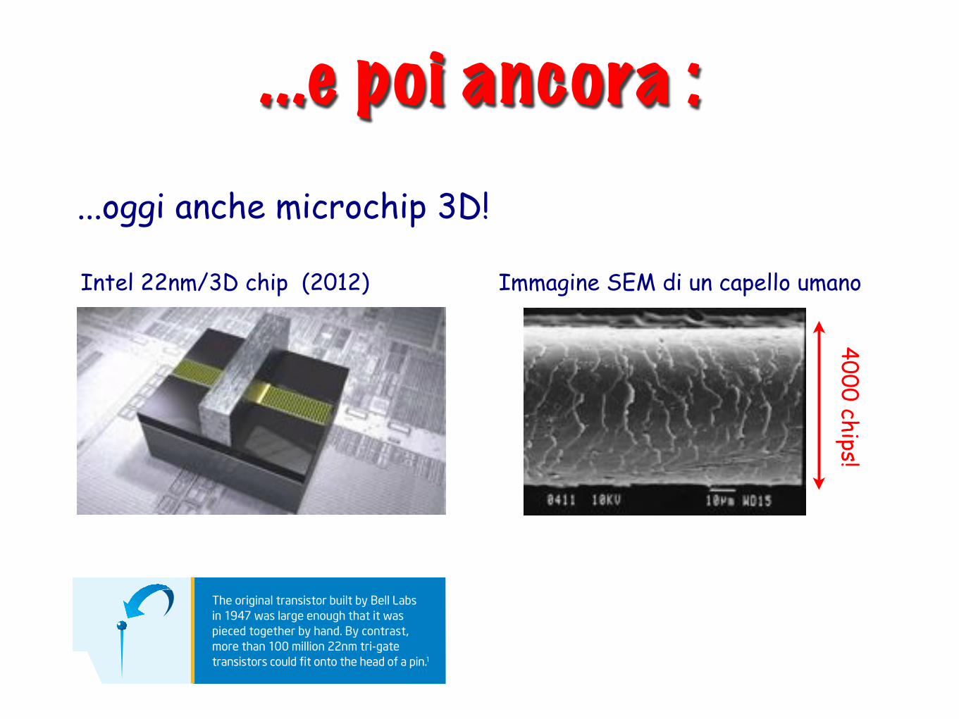
...e poi ancora :...oggi anche microchip 3D!

Intel 22nm/3D chip (2012) Immagine SEM di un capello umano

4000 chips!

Fun FactsExactly how small (and cool) is 22 Nanometers?

1 A pin head is about 1.5 mm in diameter. 2 A period is estimated to be 1/10 square millimeter in area. 3 A human hair is about 90 microns in diameter. 4 The smallest feature visible to the naked eye is 40 microns. 5�$VVXPHV�D�SHUVRQ�FDQ�ÀLFN�D�OLJKW�VZLWFK�RQ�DQG�RII�����WLPHV�SHU�PLQXWH��� �&RS\ULJKW��������,QWHO�&RUSRUDWLRQ��$OO�ULJKWV�UHVHUYHG��,QWHO�DQG�WKH�,QWHO�ORJR� DUH�WUDGHPDUNV�RI�,QWHO�&RUSRUDWLRQ�LQ�WKH�8�6��DQG�RU�RWKHU�FRXQWULHV�

*Other names and brands may be claimed as the property of others.� ������70�/$,�3')������������86

According to Moore’s Law, the number of transistors on a chip roughly doubles every two years. As a result the scale gets smaller and transistor count increases at a regular pace to provide improvements in integrated circuit functionality and performance while decreasing costs. Intel made a radical change in its transistor design in 2011, and then WKH�ZRUOG·V�ÀUVW���QP���'�WUL�JDWH�silicon transistors entered high volume production in 2012.

,QWHO���QP���'�WUDQVLVWRUV�ZLOO�GHOLYHU�an unprecedented combination of SHUIRUPDQFH�DQG�HQHUJ\�HIÀFLHQF\�in a whole range of computers, from servers to desktops, and from laptops to handheld devices.

Enjoy these facts illustrating the change in transistor size and structure, that are delivering the EHQHÀWV�RI�0RRUH·V�/DZ�WR�\RX�

The original transistor built by Bell Labs in 1947 was large enough that it was pieced together by hand. By contrast, PRUH�WKDQ�����PLOOLRQ���QP�WUL�JDWH�WUDQVLVWRUV�FRXOG�ÀW�RQWR�WKH�KHDG�RI�D�SLQ�1

0RUH�WKDQ���PLOOLRQ���QP�WUL�JDWH� WUDQVLVWRUV�FRXOG�ÀW�LQ�WKH�SHULRG�DW� the end of this sentence.2

$���QP�WUL�JDWH�WUDQVLVWRU·V�JDWHV�DUH� VR�VPDOO�\RX�FRXOG�ÀW�PRUH�WKDQ� 4,000 of them across the width of a human hair.�

If a typical house shrunk as transistors have, you would not be able to see a house without a microscope. To see a 22nm feature with the naked eye, you would have to enlarge a chip to be larger than a house.4

&RPSDUHG�WR�,QWHO·V�ÀUVW�PLFURSURFHVVRU�� the 4004, introduced in 1971, a 22nm CPU runs over 4,000 times as fast and each transistor uses about 5,000 times less energy. The price per transistor has dropped by a factor of about 50,000.

A 22nm transistor can switch on and off well over 100 billion times in one second. It would take you around 2,000 \HDUV�WR�ÁLFN�D�OLJKW�VZLWFK�RQ�DQG�RII� that many times.5

,W·V�RQH�WKLQJ�WR�GHVLJQ�D�WUL�JDWH� transistor but quite another to get it into high volume manufacturing. Intel’s factories produce over 5 billion transistors every second. That’s 150,000,000,000,000,000 transistors per year, the equivalent of over 20 million transistors for every man, woman and child on earth.

7KH��UG�*HQHUDWLRQ�,QWHO��&RUH��processor — quad core, contains 1.48 billion transistors. If transistors were people, Intel’s chip has more transistors than the population of China at DSSUR[LPDWHO\�����ELOOLRQ�SHRSOH�

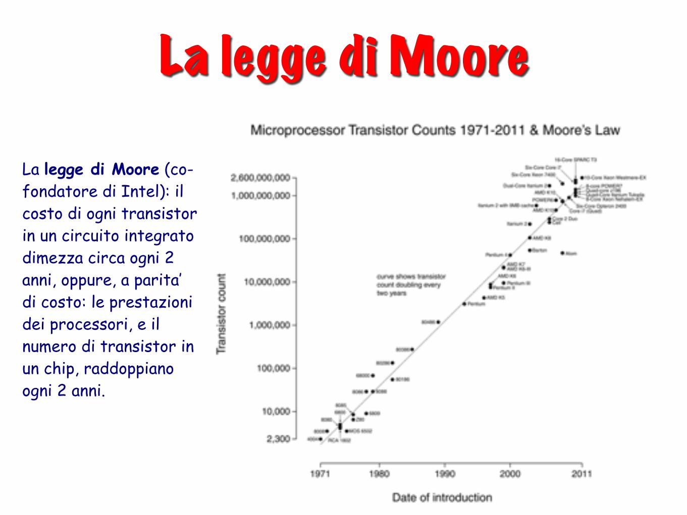
La legge di Moore

La legge di Moore (co-fondatore di Intel): il costo di ogni transistor in un circuito integrato dimezza circa ogni 2 anni, oppure, a parita’ di costo: le prestazioni dei processori, e il numero di transistor in un chip, raddoppiano ogni 2 anni.

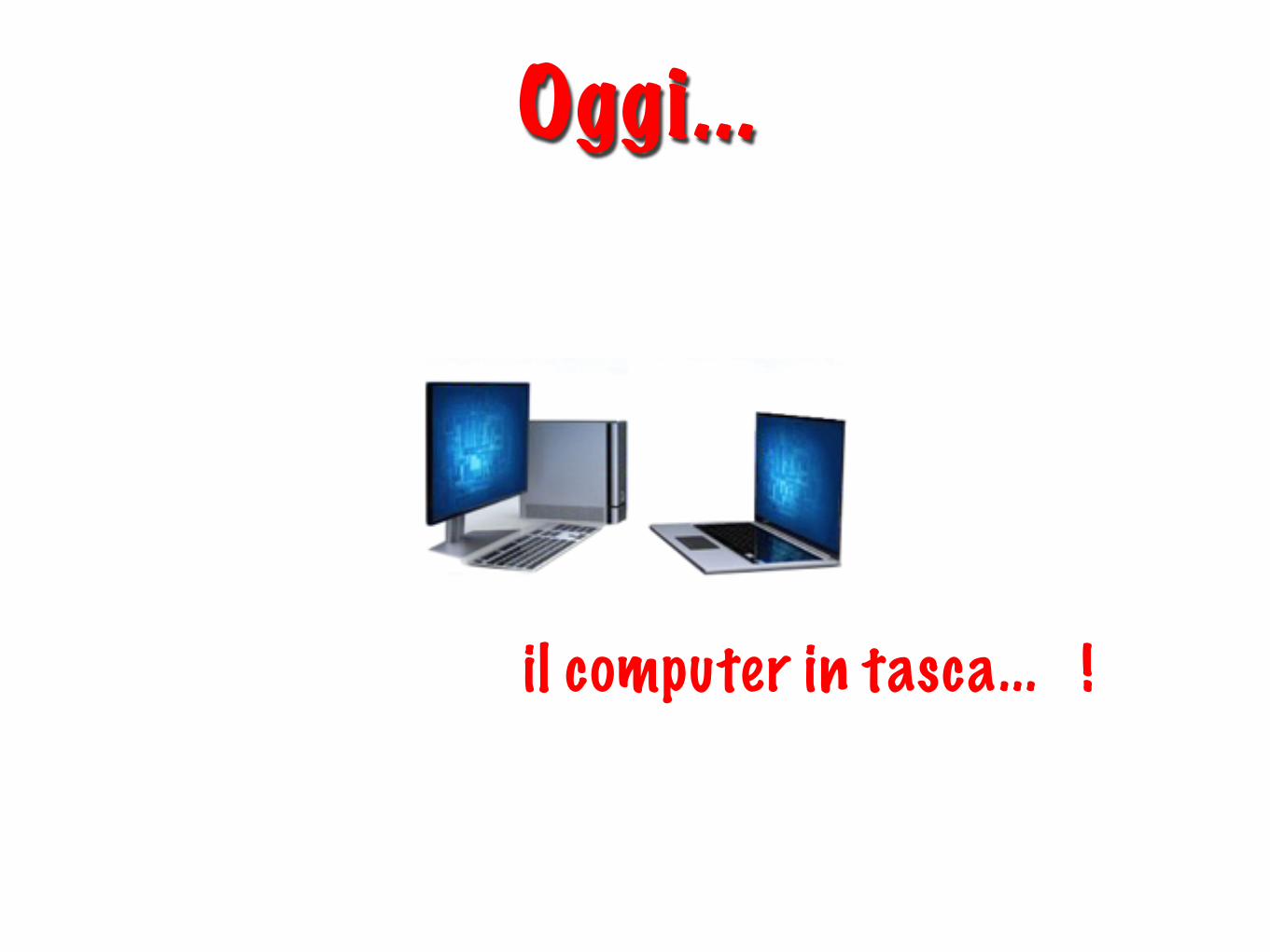
Oggi...

il computer in tasca... !

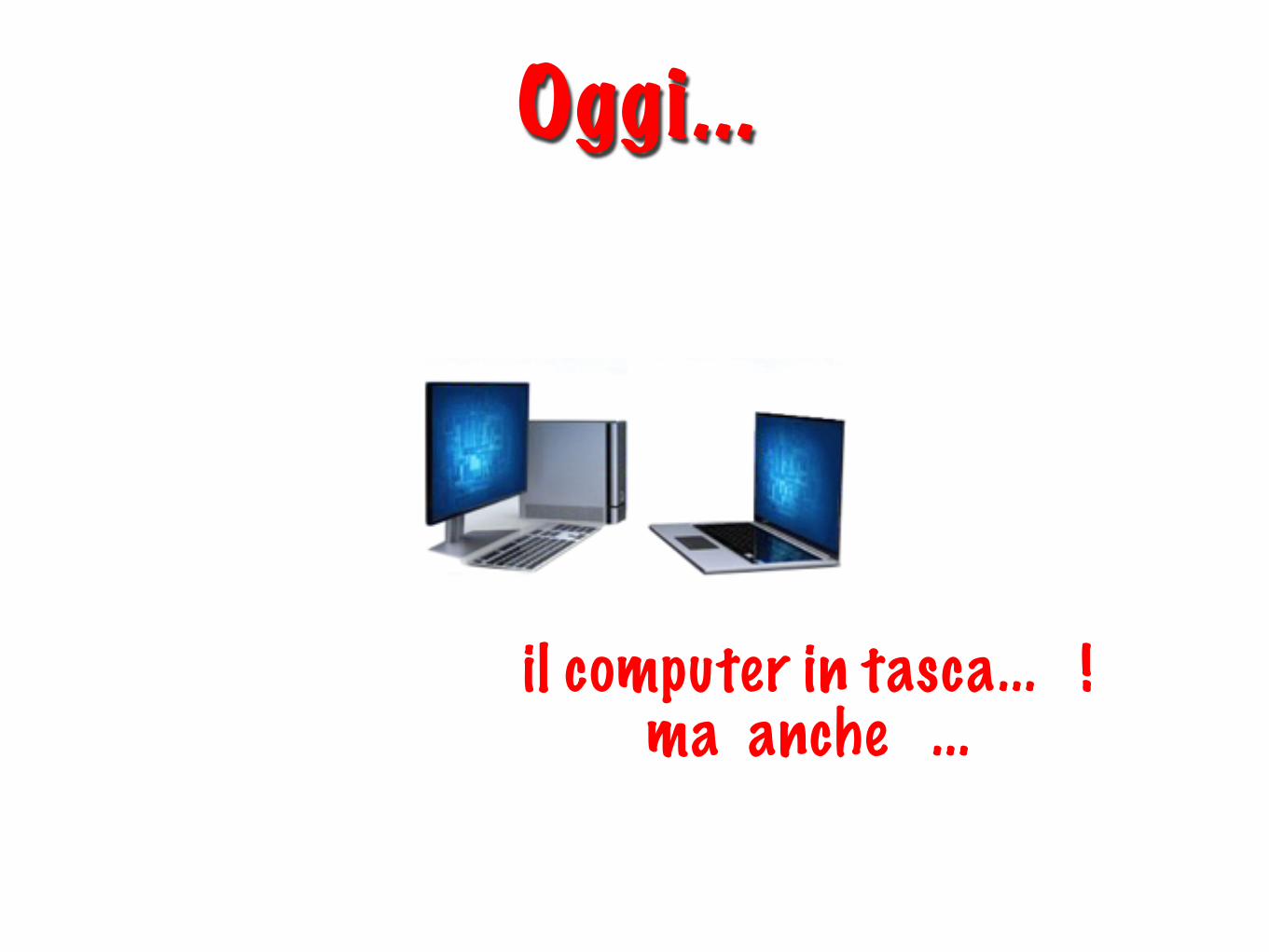
Oggi...

il computer in tasca... !ma anche ...

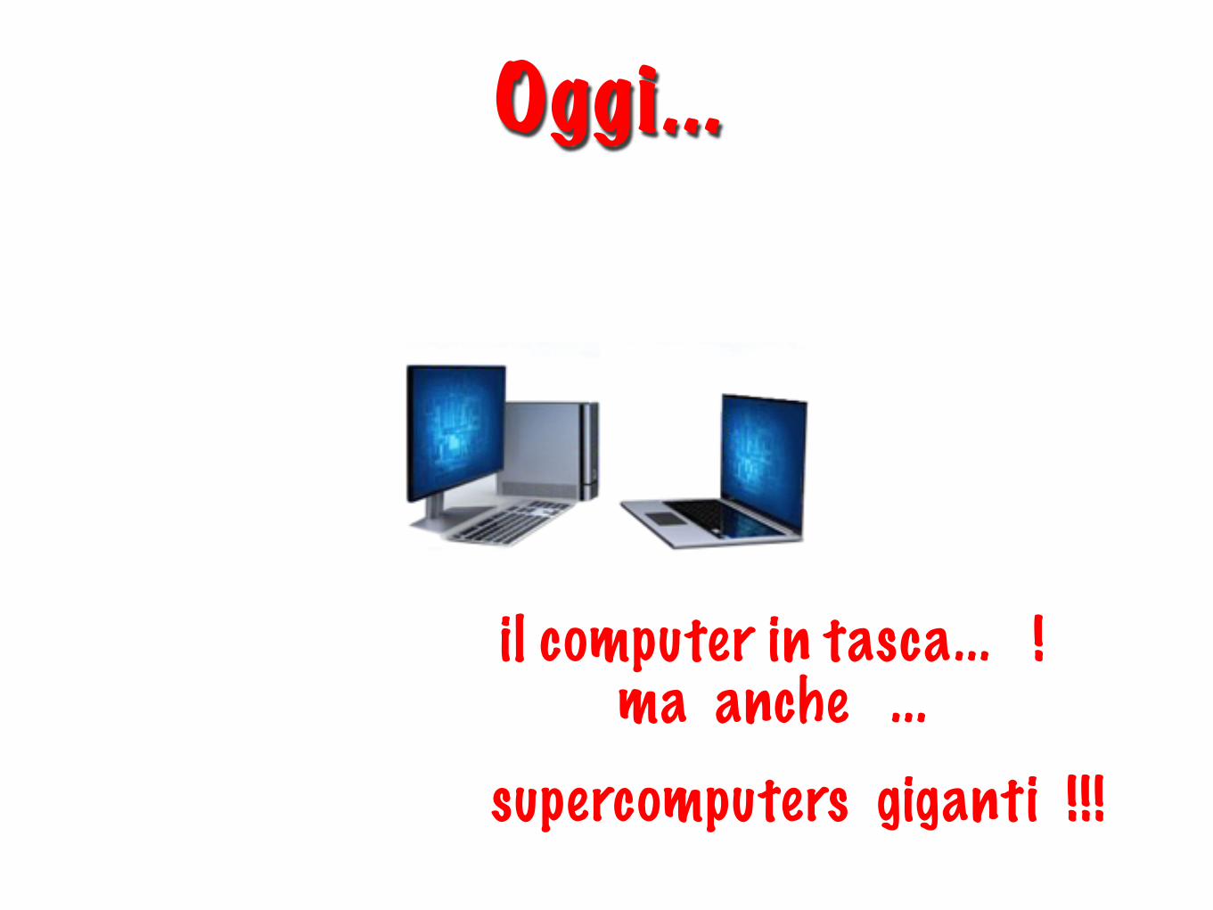
Oggi...

il computer in tasca... !ma anche ...

supercomputers giganti !!!

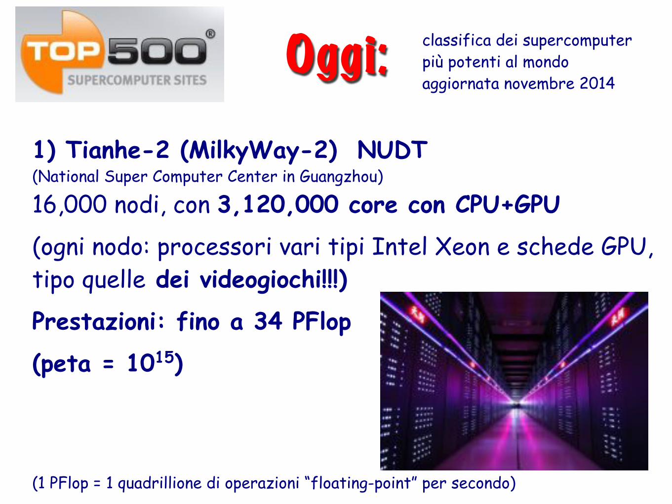
Oggi:1) Tianhe-2 (MilkyWay-2) NUDT(National Super Computer Center in Guangzhou)

16,000 nodi, con 3,120,000 core con CPU+GPU

(ogni nodo: processori vari tipi Intel Xeon e schede GPU, tipo quelle dei videogiochi!!!)

Prestazioni: fino a 34 PFlop

(peta = 1015)

(1 PFlop = 1 quadrillione di operazioni “floating-point” per secondo)

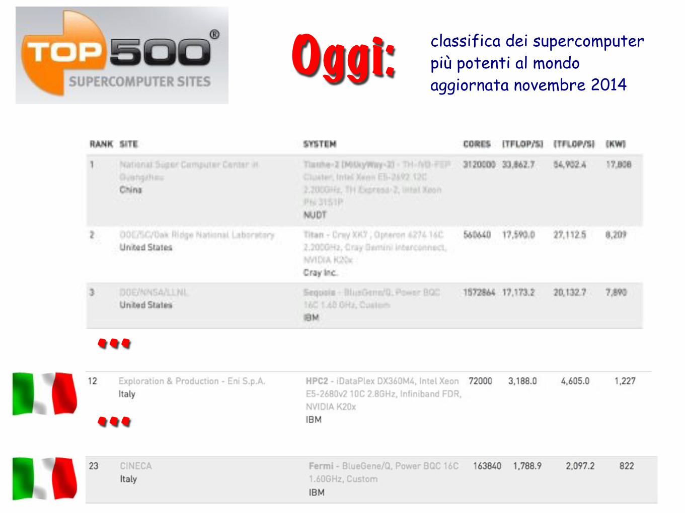
classifica dei supercomputer più potenti al mondoaggiornata novembre 2014

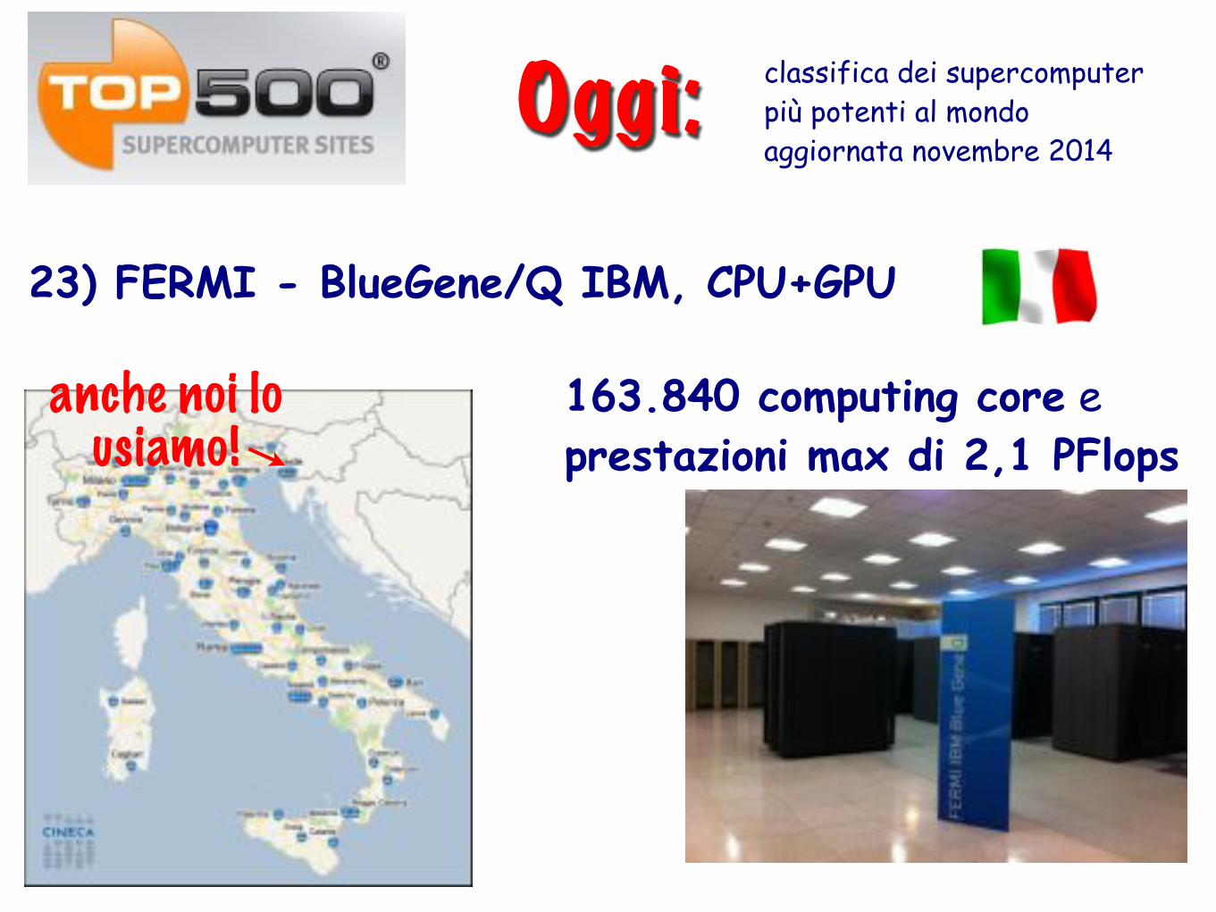
163.840 computing core e prestazioni max di 2,1 PFlops

classifica dei supercomputer più potenti al mondoaggiornata novembre 2014

23) FERMI - BlueGene/Q IBM, CPU+GPU

Oggi:

anche noi lo usiamo!

Oggi:

...

...

classifica dei supercomputer più potenti al mondoaggiornata novembre 2014

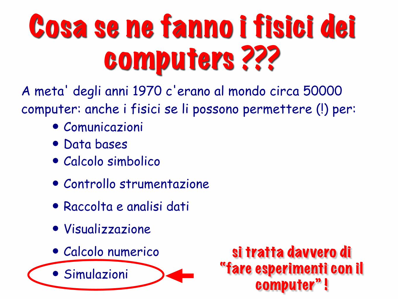
A meta' degli anni 1970 c'erano al mondo circa 50000 computer: anche i fisici se li possono permettere (!) per:

• Comunicazioni• Data bases• Calcolo simbolico

• Controllo strumentazione

• Raccolta e analisi dati

• Visualizzazione

• Calcolo numerico

• Simulazionisi tratta davvero di

“fare esperimenti con il computer” !

Cosa se ne fanno i fisici dei computers ???

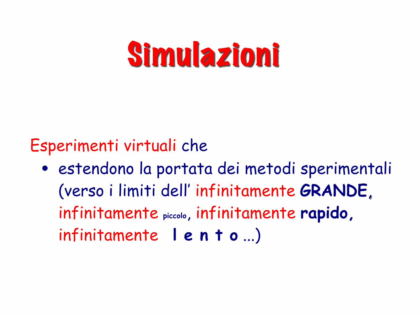
Esperimenti virtuali che• estendono la portata dei metodi sperimentali

(verso i limiti dell’ infinitamente GRANDE, infinitamente piccolo, infinitamente rapido, infinitamente l e n t o ...)

Simulazioni

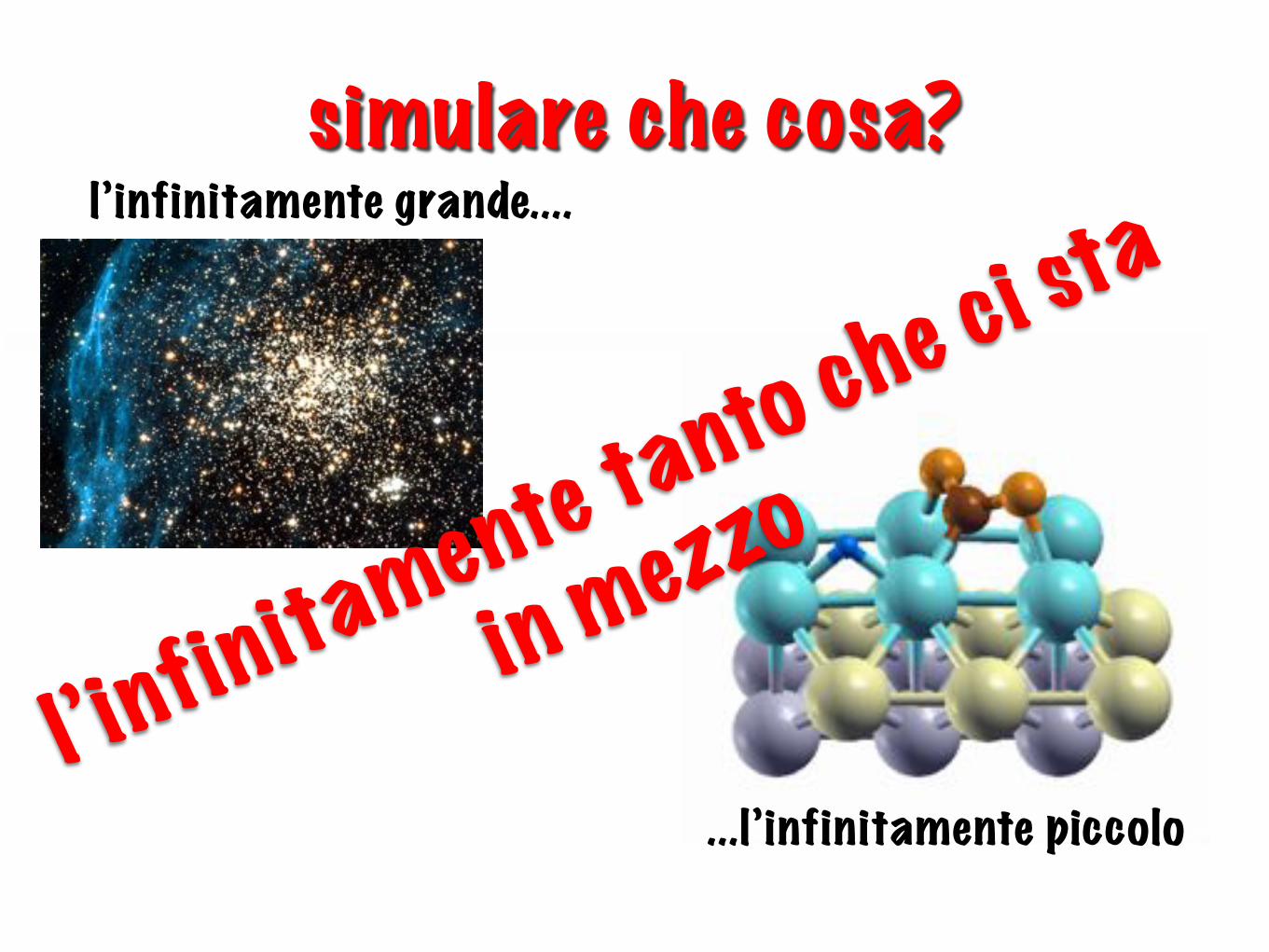
simulare che cosa?l’infinitamente grande....

...l ’infinitamente piccolol’infinitamente tanto che ci sta

in mezzo

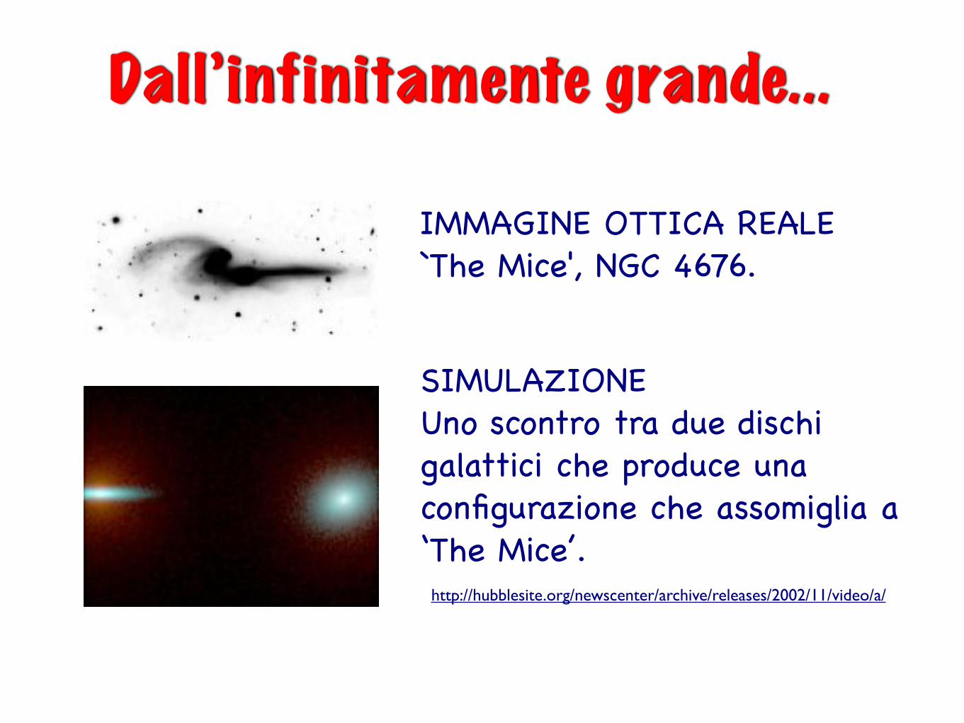
IMMAGINE OTTICA REALE`The Mice', NGC 4676.

SIMULAZIONEUno scontro tra due dischi galattici che produce una configurazione che assomiglia a ‘The Mice’.

Dall’infinitamente grande...

http://hubblesite.org/newscenter/archive/releases/2002/11/video/a/

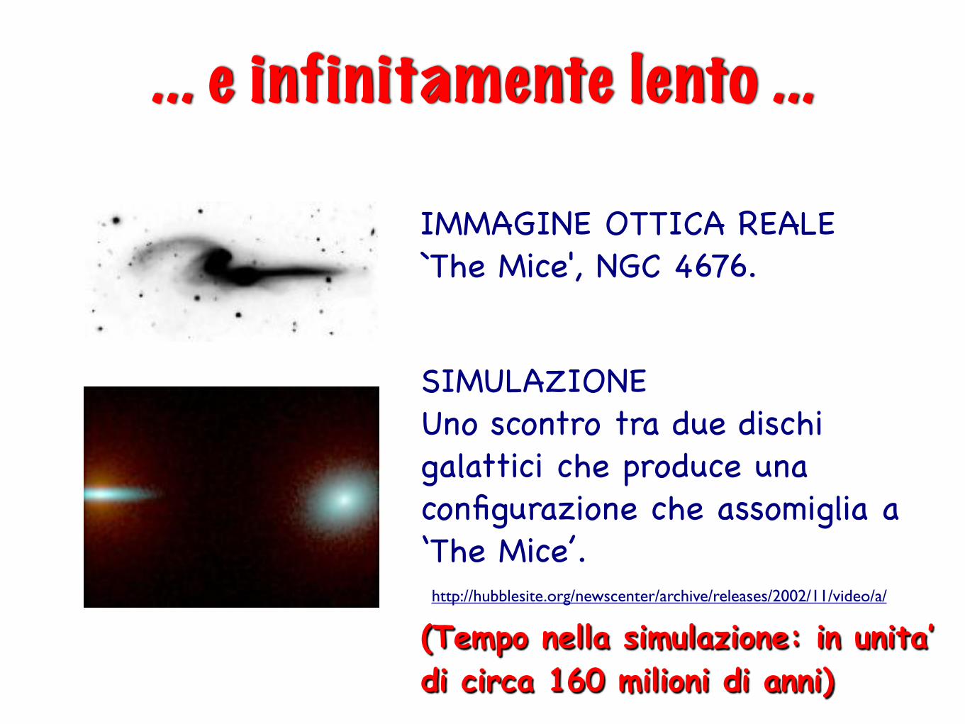
IMMAGINE OTTICA REALE`The Mice', NGC 4676.

SIMULAZIONEUno scontro tra due dischi galattici che produce una configurazione che assomiglia a ‘The Mice’.

(Tempo nella simulazione: in unita’ di circa 160 milioni di anni)

... e infinitamente lento ...

http://hubblesite.org/newscenter/archive/releases/2002/11/video/a/

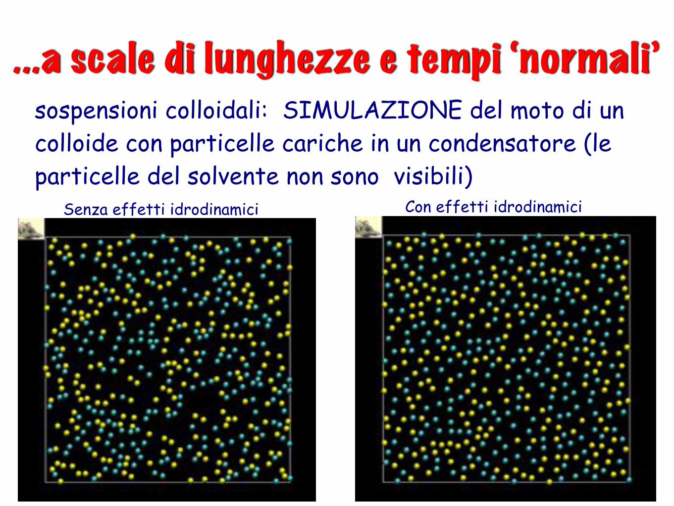
Senza effetti idrodinamici Con effetti idrodinamici

sospensioni colloidali: SIMULAZIONE del moto di un colloide con particelle cariche in un condensatore (le particelle del solvente non sono visibili)

...a scale di lunghezze e tempi ‘normali’

• perche’ ci interessa?

• quali sono i limiti dell’osservazione sperimentale?

• quali contributi puo’ dare la simulazione ?

... fin verso il limite “nano”

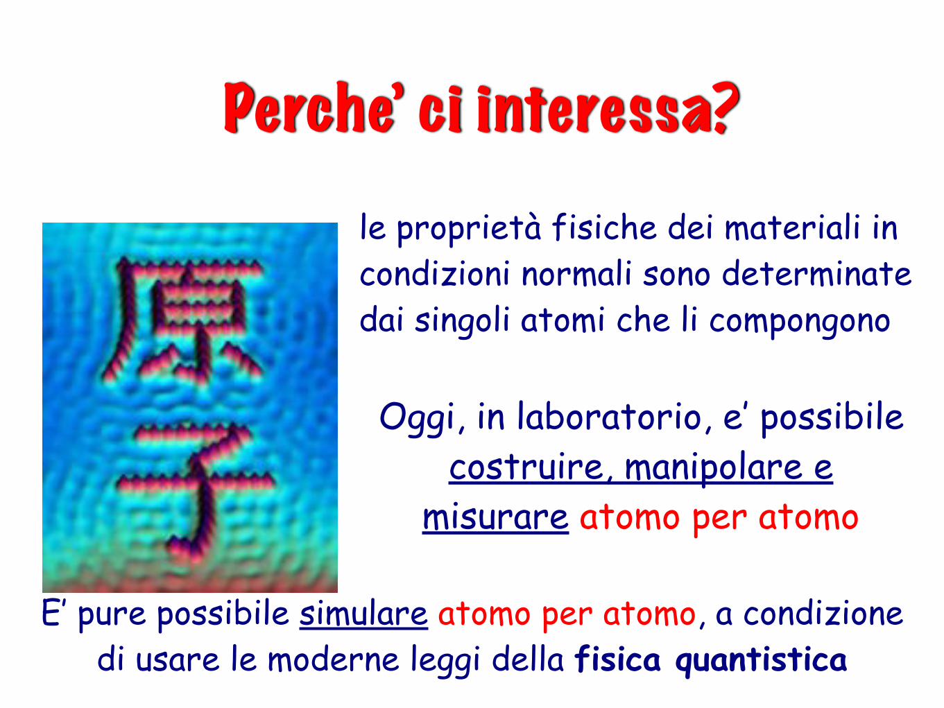
Perche’ ci interessa?

Oggi, in laboratorio, e’ possibile costruire, manipolare e

misurare atomo per atomo

le proprietà fisiche dei materiali in condizioni normali sono determinate dai singoli atomi che li compongono

E’ pure possibile simulare atomo per atomo, a condizione di usare le moderne leggi della fisica quantistica

Superfici e catalisi

simulazione

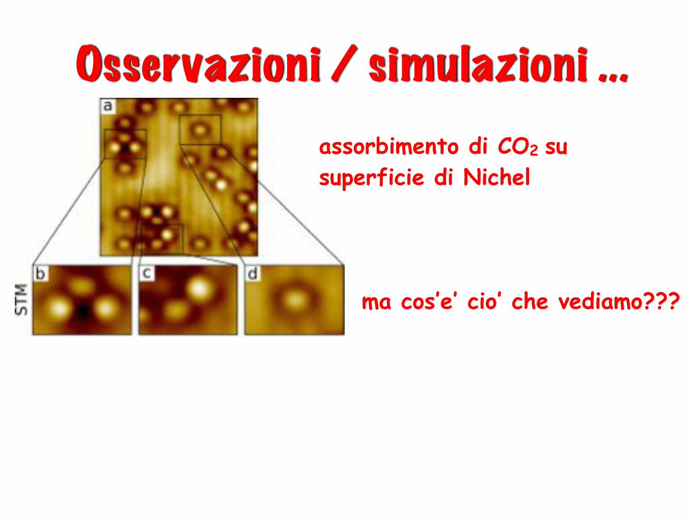
Osservazioni / simulazioni ...assorbimento di CO2 su superficie di Nichel

ma cos’e’ cio’ che vediamo???

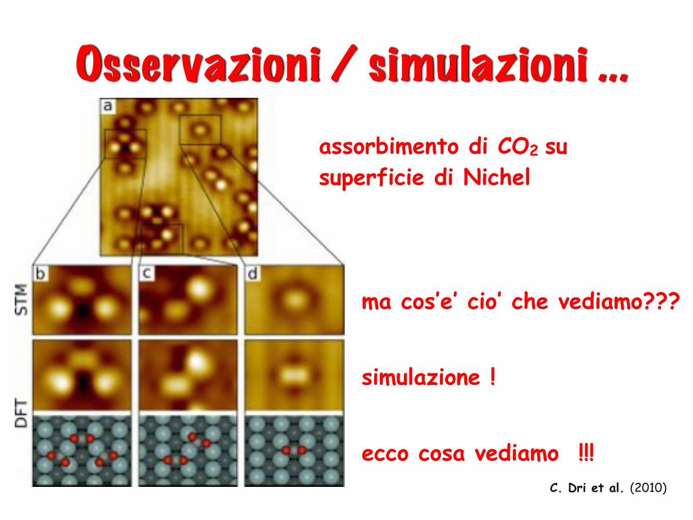
simulazione !

Osservazioni / simulazioni ...assorbimento di CO2 su superficie di Nichel

ma cos’e’ cio’ che vediamo???

ecco cosa vediamo !!!C. Dri et al. (2010)

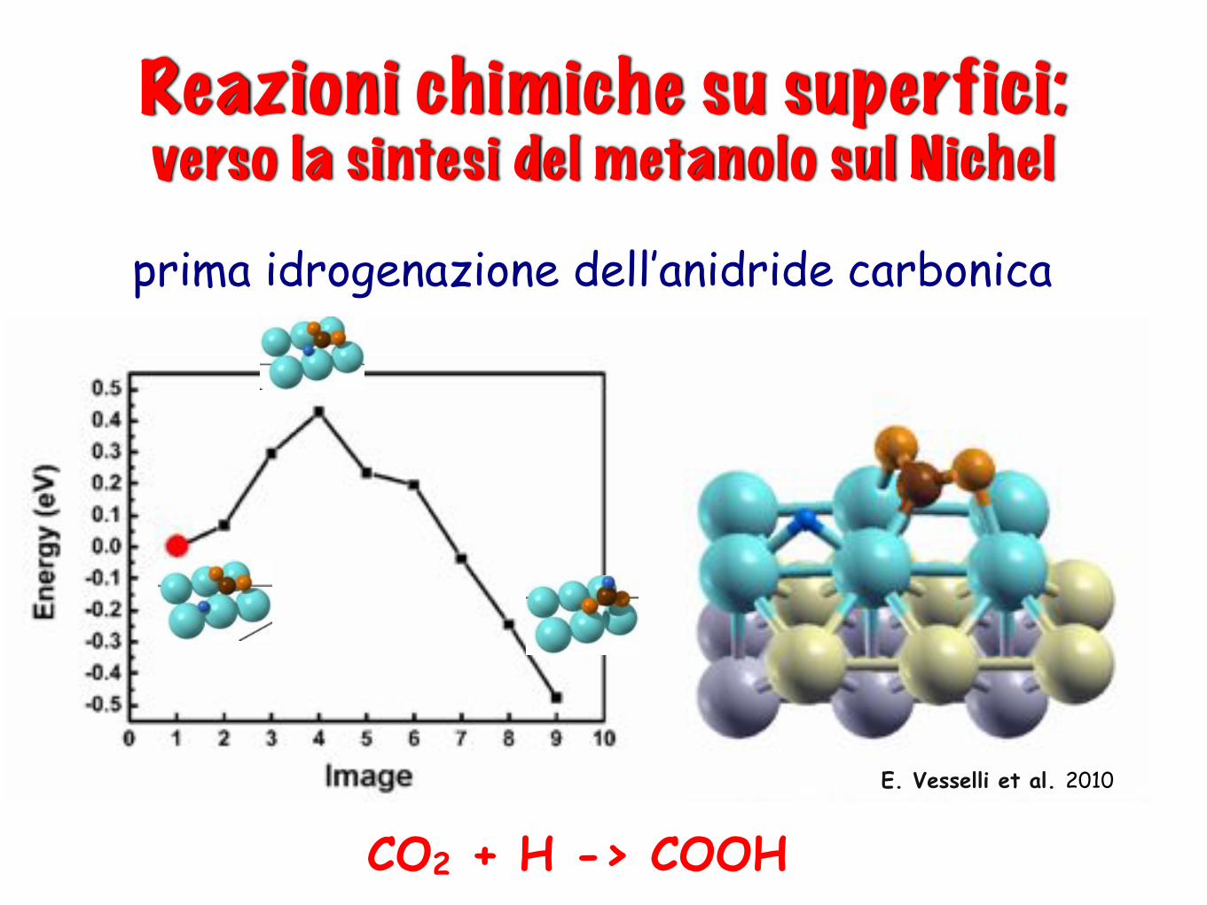
Reazioni chimiche su superfici:verso la sintesi del metanolo sul Nichel

prima idrogenazione dell’anidride carbonica

CO2 + H -> COOH

E. Vesselli et al. 2010

Nanoparticelle

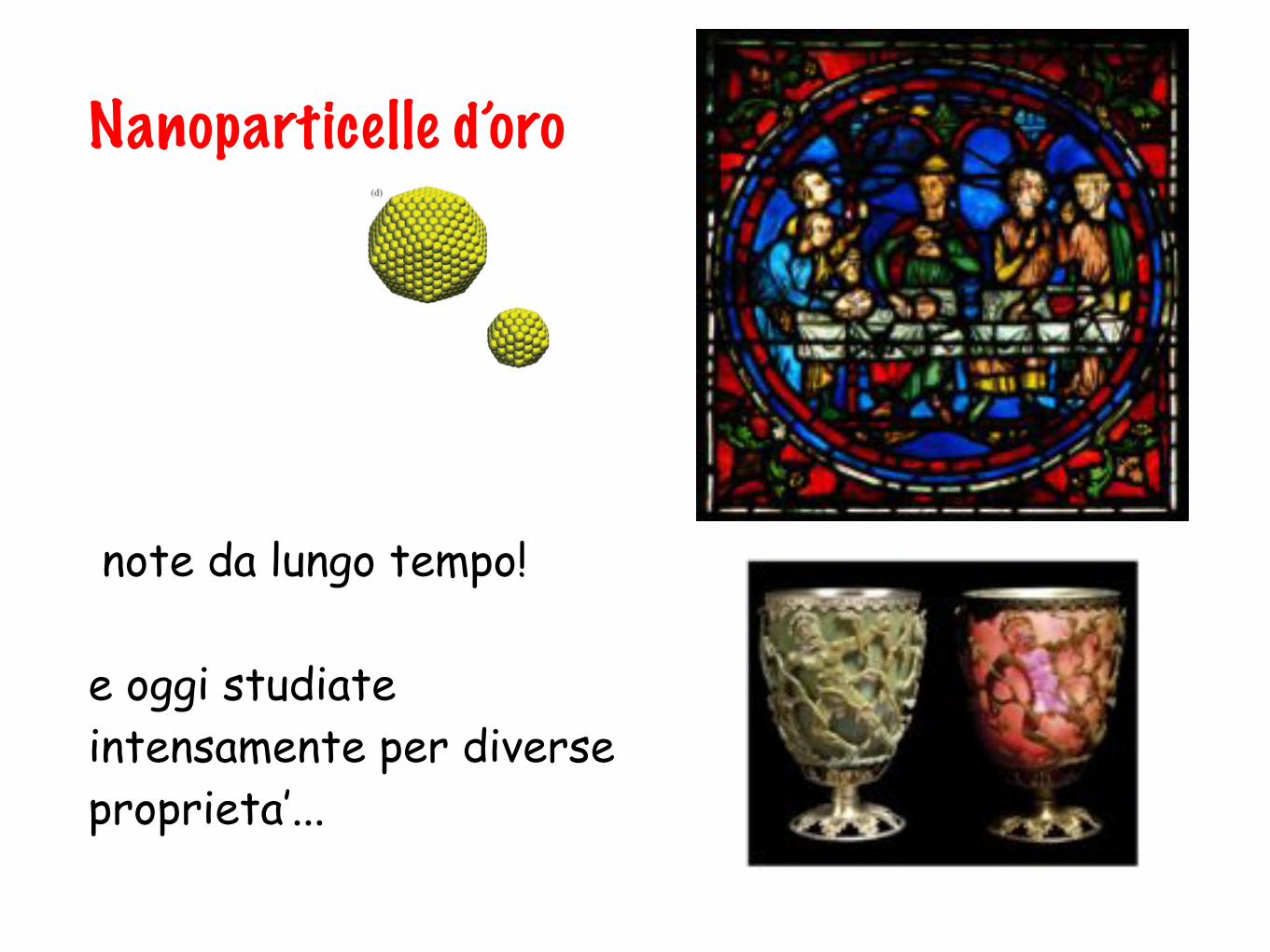
Nanoparticelle d’oro

after 1 ns. As can be seen on the figure, as the nanoparticlediameter decreases, a very strong surface disorder is observed,a phenomenon that fairly disappears as the particle sizeincreases.

For instance, in the case of Au55, the icosahedra structure iscompletely lost due to the strong S–Au interaction, comparablein magnitude to the Au–Au interaction on the outer layers ofthe gold nanoparticles (see Table 1).

At 300 K, there is a competition between perpendicularbonding (S–Au) and lateral ones (Au–Au). In Fig. 6, theatomic structure of Au147–(SR)n and Au309–(SR)n, frames (b)and (c), also reveals the formation of gold adatoms (characterized

by the low coordination number), which in most cases arebonded to one or two thiolate molecules. Several RS–Au–SRstructural motifs are formed during the LD simulation.However, due to the fact that thermal e!ects are present inour simulation model, a well-defined structure cannot becaptured. In the case of Au923–(SR)n the surface of the particleappears slightly disordered, but the internal core keeps theicosahedra structure. A remarkable feature of all of thesesimulations is the self-assembly of the alkane chains due tothe collective van der Waals interactions.It is interesting to point out the agreement of our results to

those reported by Garzon et al.,35 where by means of DFTcalculations, they have found that the e!ect of a methylthiolmonolayer, approximately 24 SCH3 molecules on a Au38cluster, is strong enough to produce a dramatic distortion onthe gold cluster, resulting in a disordered geometry for themost stable Au38(SCH3)24 capped nanoparticle.Closer inspection of the atomic configurations, by means of

computing the pair distribution function, reveals a contractionof the Au–Au distance, with respect to the equilibrium Au–Audistance in bare clusters, as the particle size decreases. Fig. 7shows the first nearest neighbor’s distribution of Au–Aubonds for the first four members of the icosahedra family.As can be observed in Fig. 7, the maximum of the peak is

displaced to lower values as the nanoparticle diameterdecreases. It is interesting to note that when the diameter ofthe nanoparticles is around 2.2 nm (B309 atoms) the Au–Aucontraction is released, due to the many-body character of themetallic bond.

Conclusions

In the present study we have shown theoretical evidenceconfirming the strong surface disorder on the structure ofthiol protected gold nanoparticles in the range 1–4 nm. Thehigh resolution electron microscopy images obtained were inagreement with the theory proposed revealing that when thenanoparticles size is lower than 2–3 nm the surface of the

Fig. 6 Initial (left) and last (right) configurations taken from the

Langevin dynamics simulation after adsorption of butanethiolate

molecules. (a) Au55–(SR)n, (b) Au147–(SR)n, (c) Au309–(SR)n,

(d) Au923–(SR)n at 300 K. See the text for details. (Yellow spheres:

Au atoms, red: S and silver bars: alkane-chain.)

Table 1 Internal energy of gold atoms on di!erent sites according tothe Second Moment Tight Binding potential (SMTB) and bindingenergy of S–Au on flat (111) surface and on-top Au adatoms accordingto our potential

Site Energy/eV

Au on Au(111) facets !3.44Au on borders !3.12S–Au(111) !1.84S–Au(adatom) !2.93

Fig. 7 Nearest neighbor’s distribution for 1-butanethiol capped gold

nanoparticles (dashed red lines) and bare gold NPs (full black line) for

di!erent core sizes (Au13, Au55, Au147, Au309). Langevin dynamics

conditions: 300 K and x = 100 ps!1.

This journal is "c the Owner Societies 2010 Phys. Chem. Chem. Phys., 2010, 12, 11785–11790 | 11789

Publ

ished

on

09 A

ugus

t 201

0. D

ownl

oade

d by

Uni

vers

ita S

tudi

di T

rieste

on

14/0

4/20

14 0

9:41

:06.

View Article Online

after 1 ns. As can be seen on the figure, as the nanoparticlediameter decreases, a very strong surface disorder is observed,a phenomenon that fairly disappears as the particle sizeincreases.

For instance, in the case of Au55, the icosahedra structure iscompletely lost due to the strong S–Au interaction, comparablein magnitude to the Au–Au interaction on the outer layers ofthe gold nanoparticles (see Table 1).

At 300 K, there is a competition between perpendicularbonding (S–Au) and lateral ones (Au–Au). In Fig. 6, theatomic structure of Au147–(SR)n and Au309–(SR)n, frames (b)and (c), also reveals the formation of gold adatoms (characterized

by the low coordination number), which in most cases arebonded to one or two thiolate molecules. Several RS–Au–SRstructural motifs are formed during the LD simulation.However, due to the fact that thermal e!ects are present inour simulation model, a well-defined structure cannot becaptured. In the case of Au923–(SR)n the surface of the particleappears slightly disordered, but the internal core keeps theicosahedra structure. A remarkable feature of all of thesesimulations is the self-assembly of the alkane chains due tothe collective van der Waals interactions.It is interesting to point out the agreement of our results to

those reported by Garzon et al.,35 where by means of DFTcalculations, they have found that the e!ect of a methylthiolmonolayer, approximately 24 SCH3 molecules on a Au38cluster, is strong enough to produce a dramatic distortion onthe gold cluster, resulting in a disordered geometry for themost stable Au38(SCH3)24 capped nanoparticle.Closer inspection of the atomic configurations, by means of

computing the pair distribution function, reveals a contractionof the Au–Au distance, with respect to the equilibrium Au–Audistance in bare clusters, as the particle size decreases. Fig. 7shows the first nearest neighbor’s distribution of Au–Aubonds for the first four members of the icosahedra family.As can be observed in Fig. 7, the maximum of the peak is

displaced to lower values as the nanoparticle diameterdecreases. It is interesting to note that when the diameter ofthe nanoparticles is around 2.2 nm (B309 atoms) the Au–Aucontraction is released, due to the many-body character of themetallic bond.

Conclusions

In the present study we have shown theoretical evidenceconfirming the strong surface disorder on the structure ofthiol protected gold nanoparticles in the range 1–4 nm. Thehigh resolution electron microscopy images obtained were inagreement with the theory proposed revealing that when thenanoparticles size is lower than 2–3 nm the surface of the

Fig. 6 Initial (left) and last (right) configurations taken from the

Langevin dynamics simulation after adsorption of butanethiolate

molecules. (a) Au55–(SR)n, (b) Au147–(SR)n, (c) Au309–(SR)n,

(d) Au923–(SR)n at 300 K. See the text for details. (Yellow spheres:

Au atoms, red: S and silver bars: alkane-chain.)

Table 1 Internal energy of gold atoms on di!erent sites according tothe Second Moment Tight Binding potential (SMTB) and bindingenergy of S–Au on flat (111) surface and on-top Au adatoms accordingto our potential

Site Energy/eV

Au on Au(111) facets !3.44Au on borders !3.12S–Au(111) !1.84S–Au(adatom) !2.93

Fig. 7 Nearest neighbor’s distribution for 1-butanethiol capped gold

nanoparticles (dashed red lines) and bare gold NPs (full black line) for

di!erent core sizes (Au13, Au55, Au147, Au309). Langevin dynamics

conditions: 300 K and x = 100 ps!1.

This journal is "c the Owner Societies 2010 Phys. Chem. Chem. Phys., 2010, 12, 11785–11790 | 11789

Publ

ished

on

09 A

ugus

t 201

0. D

ownl

oade

d by

Uni

vers

ita S

tudi

di T

rieste

on

14/0

4/20

14 0

9:41

:06.

View Article Online

note da lungo tempo!

e oggi studiate intensamente per diverse proprieta’...

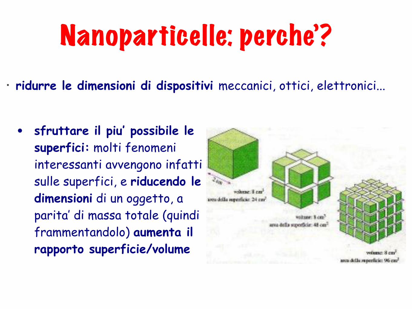
• sfruttare il piu’ possibile le superfici: molti fenomeni interessanti avvengono infatti sulle superfici, e riducendo le dimensioni di un oggetto, a parita’ di massa totale (quindi frammentandolo) aumenta il rapporto superficie/volume

Nanoparticelle: perche’?• ridurre le dimensioni di dispositivi meccanici, ottici, elettronici...

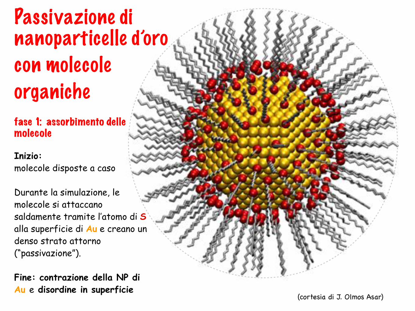
fase 1: assorbimento delle molecole

Inizio: molecole disposte a caso

Durante la simulazione, le molecole si attaccano saldamente tramite l’atomo di S alla superficie di Au e creano un denso strato attorno (“passivazione”).

Fine: contrazione della NP di Au e disordine in superficie

(cortesia di J. Olmos Asar)

Passivazione di nanoparticelle d’oro con molecole organiche

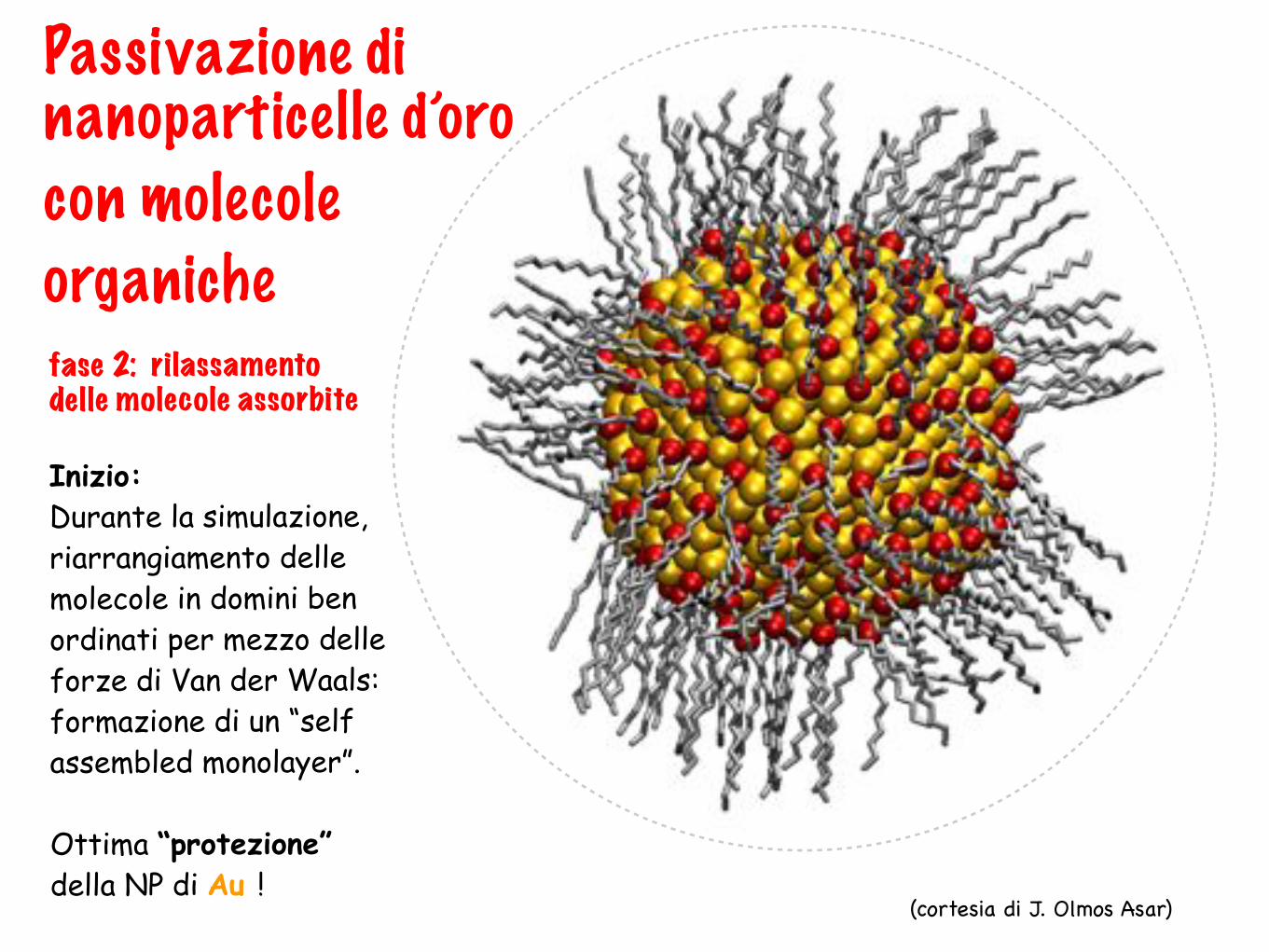
fase 2: rilassamento delle molecole assorbite

Inizio:Durante la simulazione, riarrangiamento delle molecole in domini ben ordinati per mezzo delle forze di Van der Waals:formazione di un “self assembled monolayer”.

Ottima “protezione” della NP di Au !

(cortesia di J. Olmos Asar)

Passivazione di nanoparticelle d’oro con molecole organiche

nanoparticles was highly disordered. In addition, when thegold clusters were smaller than 2 nm, a crystalline structurecould not be resolved. Evidence of small Au nucleus andisolated adatoms and chain of gold with unusual Au–Audistances were also observed.

Langevin dynamics simulations using a new semi-empiricalapproach to realistically describe the complex S–Au energylandscape are used to explore the structure of butanethiolatecapped Au nanoparticles, in the range 1–4 nm. In generalterms, a very good agreement has been found between thestructures of the synthesized nanoparticles and that simulated.For a direct comparison, in Fig. 8, two Au nanoparticles ofsimilar size are shown. As can be seen the structure of theparticles presents the same structural behavior, i.e. a strongsurface disorder with the formation of Au ad atoms.

Acknowledgements

M.M.M. wishes to thank CONICET, Welch foundationagency project #AX-1615, to the ICNAM of the Universityof Texas, Secyt-UNC, Program BID (PICT 2007-00340,2006-0946 and PME 2006-1581) for financial support.J.A.O.-A. thanks CONICET for the fellowship. The authorswould also like to thank Dr Larry F. Allard for technicalsupport.

Notes and references

1 A. Manna, T. Imae, K. Aoi and M. Okazaki, Mol. Simul., 2003,29, 661–665.

2 R. Hong, G. Han, J. M. Fernandez, B. Kim, N. S. Forbes andV. M. Rotello, J. Am. Chem. Soc., 2006, 128, 1078–1079.

3 M. M. Mariscal and S. A. Dassie, Recent Advances in Nanoscience,Research Signpost Pub., Trivandrum, India, 2007.

4 A. Ulman, S. D. Evans, Y. Shnidman, R. Sharma, E. Eilers andJ. C. Chang, J. Am. Chem. Soc., 1991, 113, 1499–1506.

5 D. J. Lavrich, S. M. Wetterer, S. L. Bernasek and G. Scoles,J. Phys. Chem. B, 1998, 102, 3456–3465.

6 C. Vericat, G. A. Benitez, D. E. Grumelli, M. E. Vela andR. C. Salvarezza, J. Phys.: Condens. Matter, 2008, 20,184004.

7 J. Hautman and M. Klein, J. Chem. Phys., 1989, 91, 4994–5001.8 A. Pertsin and M. Grunze, Langmuir, 1994, 10, 3668–3674.9 Y. Yourdshahyan and A. M. Rappe, J. Chem. Phys., 2002, 117,825–833.

10 M. J. Esplandiu, M. L. Carot, F. P. Cometto, V. A. Macagno andE. M. Patrito, Surf. Sci., 2006, 600, 155–172.

11 W. D. Luedtke and U. Landman, J. Phys. Chem., 1996, 100,13323–13329.

12 P. D. Jadzinsky, G. Calero, C. J. Ackerson, D. A. Bushnell andR. D. Kornberg, Science, 2007, 318, 430–433.

13 A. Cossaro, R. Mazzarello, R. Rousseau, L. Casalis, A. Verdini,A. Kohlmeyr, L. Floreano, S. Scandolo, A. Morgante, M. L. Kleinand G. Scoles, Science, 2008, 321, 943–946.

14 Y. Li, G. Galli and F. Gygi, ACS Nano, 2008, 2, 1896–1902.15 M. W. Heaven, A. Dass, P. S. White, K. M. Holt and

R. W. Murray, J. Am. Chem. Soc., 2008, 130, 3754–3755.16 J. Akola, M. Walter, R. L. Whetten, H. Hakkinen and

H. Gronbeck, J. Am. Chem. Soc., 2008, 130, 3756–3757.17 B. J. Henz, T. Hawa and M. R. Zachariah, Langmuir, 2008, 24,

773–783.18 N. Gonzalez-Lakunza, N. Lorente and A. Arnau, J. Phys. Chem.

C, 2007, 111, 12383–12390.19 F. P. Cometto, P. Paredes Olivera, V. A. Macagno and

E. M. Patrito, J. Phys. Chem. B, 2005, 109, 21737–21748.20 A. Bencini, G. Rajaraman, F. Totti and M. Tusa, Superlattices

Microstruct., 2009, 46, 4–9.21 R. Maha!y, R. Bhatia and B. J. Garrison, J. Phys. Chem., 1997,

101, 771–773.22 K. S. S. Liu, C. W. Yong, B. J. Garrison and J. C. Vickerman,

J. Phys. Chem. B, 1999, 103, 3195–3205.23 M. Brust, M. Walker, D. Bethell, D. J. Schi!rin and R. Whyman,

J. Chem. Soc., Chem. Commun., 1994, 801.24 C. Gutierrez-Wing, P. Santiago, J. A. Ascencio, A. Camacho and

M. J. Yacaman, Appl. Phys. A: Solid Surf., 2000, 71, 237–243.25 T. G. Schaa!, M. N. Schafigullin, J. T. Khoury, I. Vezmar,

R. L. Whetten, W. G. Cullen, P. N. First, C. Gutierrez-Wing,J. Ascencio and M. J. Jose-Yacaman, J. Phys. Chem. B, 1997, 101,7885–7891.

26 R. L. Whetten, J. T. Khoury, M. M. Alvarez, S. Murthy,I. Vezmar, Z. L. Wang, P. W. Stephens, C. L. Cleveland,W. D. Luedtke and U. Landman, Adv. Mater., 1996, 8, 428.

27 www.hremresearch.com.28 P. Maksymovych, D. C. Sorescu and J. T. Yates, Phys. Rev. Lett.,

2006, 97, 146103.29 The adsorption energy of RS/Au(100) and the staple motif

(RS–Au–SR)/Au(111) was calculated by us, using DFT/GGAwithin the e!ective core potential approach and doublez-polarization basis set.

30 D.-e. Jiang, M. L. Tiago, W. D. Luo and S. Dai, J. Am. Chem.Soc., 2008, 130, 2777–2779.

31 F. Cleri and V. Rosato, Phys. Rev. B: Condens. Matter, 1993, 48,22–33.

32 A. K. Rappe, C. J. Casewit, K. S. Colwell, W. A. Goddard III andW. M. Ski!, J. Am. Chem. Soc., 1992, 114, 10024–10035.

33 M. P. Allen and D. J. Tildesley, Computer Simulation of Liquids,Clarendon Press, Oxford, 1987.

34 J. Nocendal and S. J. Wright, Numerical Optimization, Springer,New York, 1999, p. 224.

35 I. L. Garzon, J. A. Reyes-Nava, J. I. Rodrıguez-Hernandez,I. Sigal, M. R. Beltran and K. Michaelian, Phys. Rev. B: Condens.Matter Mater. Phys., 2002, 66, 073403.

Fig. 8 A comparison between an experimental and a theoretical

structure of a gold nanoparticle capped by alkanethiol molecules of

similar size.

11790 | Phys. Chem. Chem. Phys., 2010, 12, 11785–11790 This journal is !c the Owner Societies 2010

Publ

ished

on

09 A

ugus

t 201

0. D

ownl

oade

d by

Uni

vers

ita S

tudi

di T

rieste

on

14/0

4/20

14 0

9:41

:06.

View Article Online

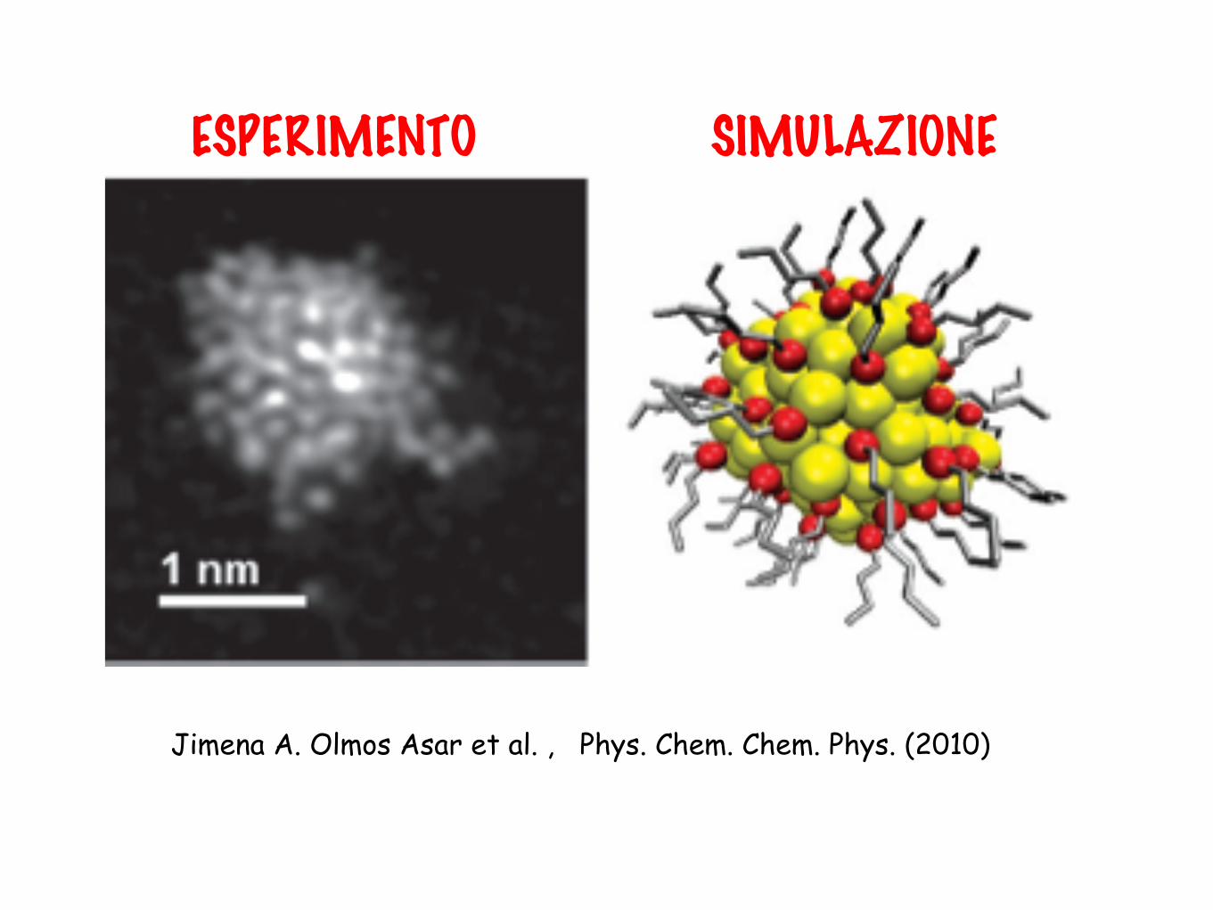
Jimena A. Olmos Asar et al. , Phys. Chem. Chem. Phys. (2010)

ESPERIMENTO SIMULAZIONE

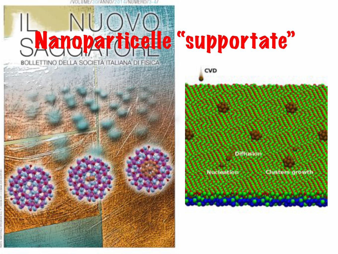
Nanoparticelle “supportate”

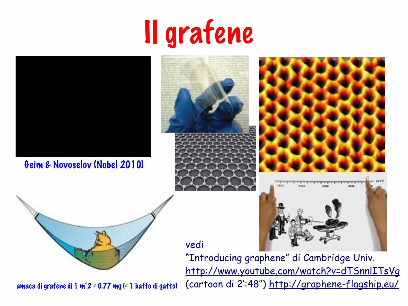
amaca di grafene di 1 m^2 = 0.77 mg (= 1 baffo di gatto)

Geim & Novoselov (Nobel 2010)

Il grafene

vedi“Introducing graphene” di Cambridge Univ.http://www.youtube.com/watch?v=dTSnnlITsVg(cartoon di 2’:48’’) http://graphene-flagship.eu/

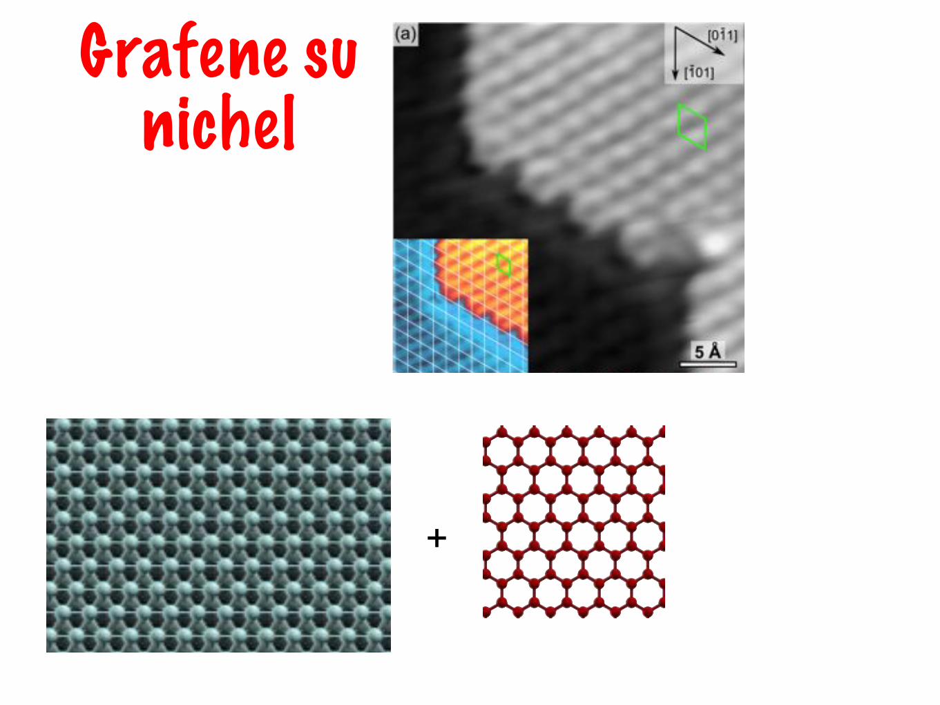
Grafene su nichel

6

Figure 1. Graphene edges on Ni(111). (a) STM image acquired at RT and showing a graphene

island (right) grown on top of a Ni terrace (left) [V=-10mV, I=20nA]. Inset: a grid intersecting

on top of the Ni atoms is drawn on a zoom in (a). A two-color scale is used to better highlight the

Ni atoms. (b) Stick-and-ball model of a graphene layer on Ni(111). Blue lines indicate cuts

passing at hollow C atoms and oriented along the six high-symmetry directions. The expected

Page 10 of 26

ACS Paragon Plus Environment

Nano Letters

123456789101112131415161718192021222324252627282930313233343536373839404142434445464748495051525354555657585960

+

La simulazione fornisce la spiegazione di come cresce il grafene sul substrato metallico di Nie il ruolo della temperatura e dell’idrogeno

suggerimento: possibile meccanismo di stoccaggio dell’idrogeno?

6

Figure 1. Graphene edges on Ni(111). (a) STM image acquired at RT and showing a graphene

island (right) grown on top of a Ni terrace (left) [V=-10mV, I=20nA]. Inset: a grid intersecting

on top of the Ni atoms is drawn on a zoom in (a). A two-color scale is used to better highlight the

Ni atoms. (b) Stick-and-ball model of a graphene layer on Ni(111). Blue lines indicate cuts

passing at hollow C atoms and oriented along the six high-symmetry directions. The expected

Page 10 of 26

ACS Paragon Plus Environment

Nano Letters

123456789101112131415161718192021222324252627282930313233343536373839404142434445464748495051525354555657585960

Grafene su nichel

• approccio deterministico

• approccio stocastico/probabilistico (metodi Monte Carlo)

...ma come si fa a fare delle simulazioni ???

Esempio: moto dei pianeti

L’approccio deterministico

conosco le equazioni che descrivono un sistema fisiconon so come risolverle con “carta e matita” (soluzione analitica);chiedo al computer di risolverle per me .... anche in maniera approssimata (soluzione numerica)

The deterministic method�

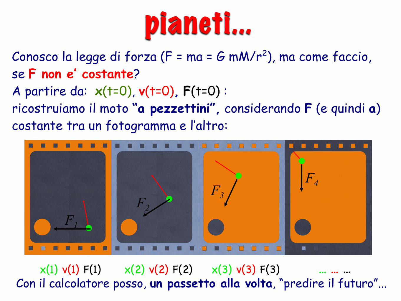
x(1) v(1) F(1) � x(2) v(2) F(2)� x(3) v(3) F(3)� ... ... …�

F1�F2�

F3�F4�

Discretization of the equation of motion and iteration: �Conosco la legge di forza (F = ma = G mM/r2), ma come faccio, se F non e’ costante? A partire da: x(t=0), v(t=0), F(t=0) : ricostruiamo il moto “a pezzettini”, considerando F (e quindi a) costante tra un fotogramma e l’altro:

pianeti...

Con il calcolatore posso, un passetto alla volta, “predire il futuro”...

!"#$%&'()*+,# ')(+&-.#+/0)&.%/&#1&2%34"*+( 5+1)0#%/+&.%/.1",#6)

!"#"$%&'$(')*&#'

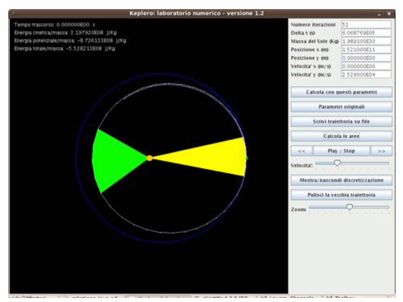
Questa applicazione calcola e visualizza il moto di un pianeta (in generale di un oggetto orbitante) attorno ad una stella. Per il calcolo, si implementa l'algoritmo di Verlet. La parte di calcolo è concentrata nella classe MotoPianeta.L'interfaccia grafica utente, descritta nella classe Keplero (la quale implementa anche il metodo main necessario per avere un programma eseguibile) dà il risultato qui riportato:

I vari campi consentono di modificare i parametri del calcolo (predefiniti: Terra intorno al Sole, con discretizzazione ad una settimana). I pulsanti permettono di effettuare una animazione dell'orbita, di cambiare i parametri di visualizzazione, di scrivere su file, di ripristinare i parametri predefiniti. Il programma consente di mostrare le ultime due traiettorie calcolate, così da confrontare direttamente il risultato di valori fisici diversi (nell'esempio sopra riportato, in blu scuro la traiettoria della Terra e in chiaro con una velocità iniziale ridotta).Le quantità fisiche più rilevanti sono visualizzate all'interno dell'area del grafico. Inoltre, un pulsante consente di effettuare il calcolo delle aree, mostrando anche graficamente l'uguaglianza dell'area spazzata in tempi uguali. Infine, è possibile esportare su file la traiettoria, incluso la velocità, l'accelerazione e l'energia cinetica e potenziale.

78&9+::()#%&7;<; =)>?&8@AB

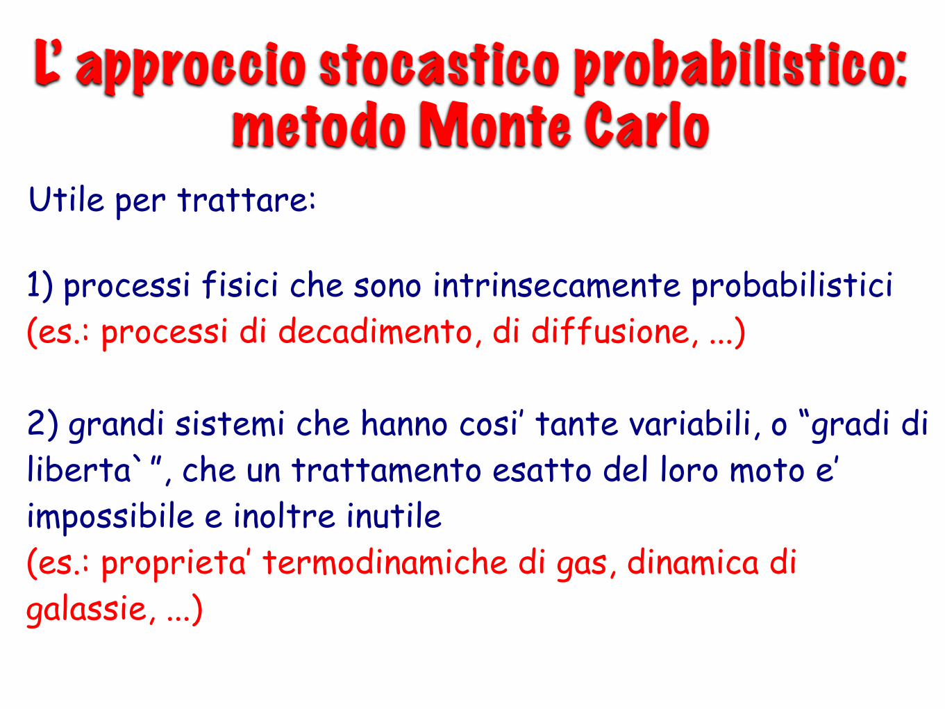
1) processi fisici che sono intrinsecamente probabilistici (es.: processi di decadimento, di diffusione, ...)

2) grandi sistemi che hanno cosi’ tante variabili, o “gradi di liberta`”, che un trattamento esatto del loro moto e’ impossibile e inoltre inutile (es.: proprieta’ termodinamiche di gas, dinamica di galassie, ...)

Utile per trattare:

L’ approccio stocastico probabilistico:metodo Monte Carlo

qualunque procedura che fa uso di variabili casuali, ossia variabili i cui valori sono aleatori

ma con una ben definita distribuzione statistica

L’ approccio stocastico probabilistico:metodo Monte Carlo

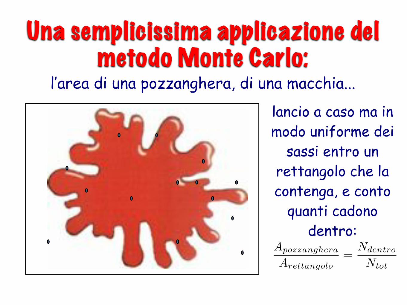
Una semplicissima applicazione delmetodo Monte Carlo:

l’area di una pozzanghera, di una macchia...

Una semplicissima applicazione delmetodo Monte Carlo:

l’area di una pozzanghera, di una macchia...

Apozzanghera

Arettangolo=

Ndentro

Ntot

lancio a caso ma in modo uniforme dei

sassi entro un rettangolo che la contenga, e conto

quanti cadono dentro:

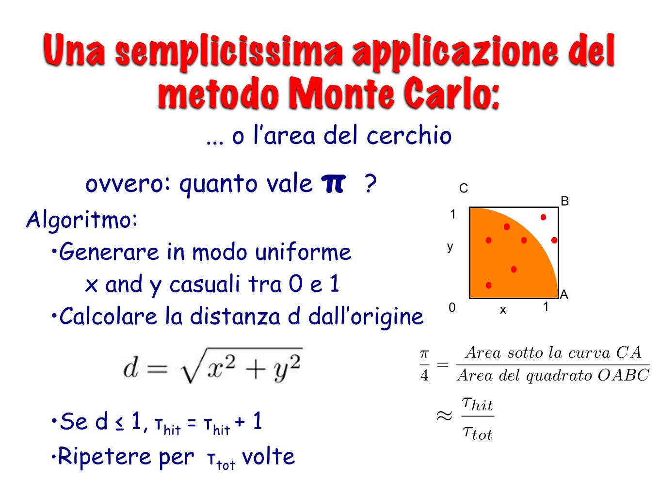
ovvero: quanto vale π ?

A1

CB

y

x0

1Algoritmo:•Generare in modo uniforme x and y casuali tra 0 e 1•Calcolare la distanza d dall’origine

•Se d ≤ 1, τhit = τhit + 1•Ripetere per τtot volte

!

!hit

!tot

!

4=

Area sotto la curva CA

Area del quadrato OABC

Una semplicissima applicazione delmetodo Monte Carlo:

... o l’area del cerchio

“fare fisica con il computer”sul fronte della scienza:

proporre modelli e meccanismi al fine di aiutare la formulazione delle leggi fondamentali della natura

spiegare le proprietà dei sistemi macroscopici a partire dalle equazioni che determinano la dinamica dei loro costituenti microscopici

sul fronte della tecnologia:

proporre materiali e dispositivi con determinate proprietà

...ma...

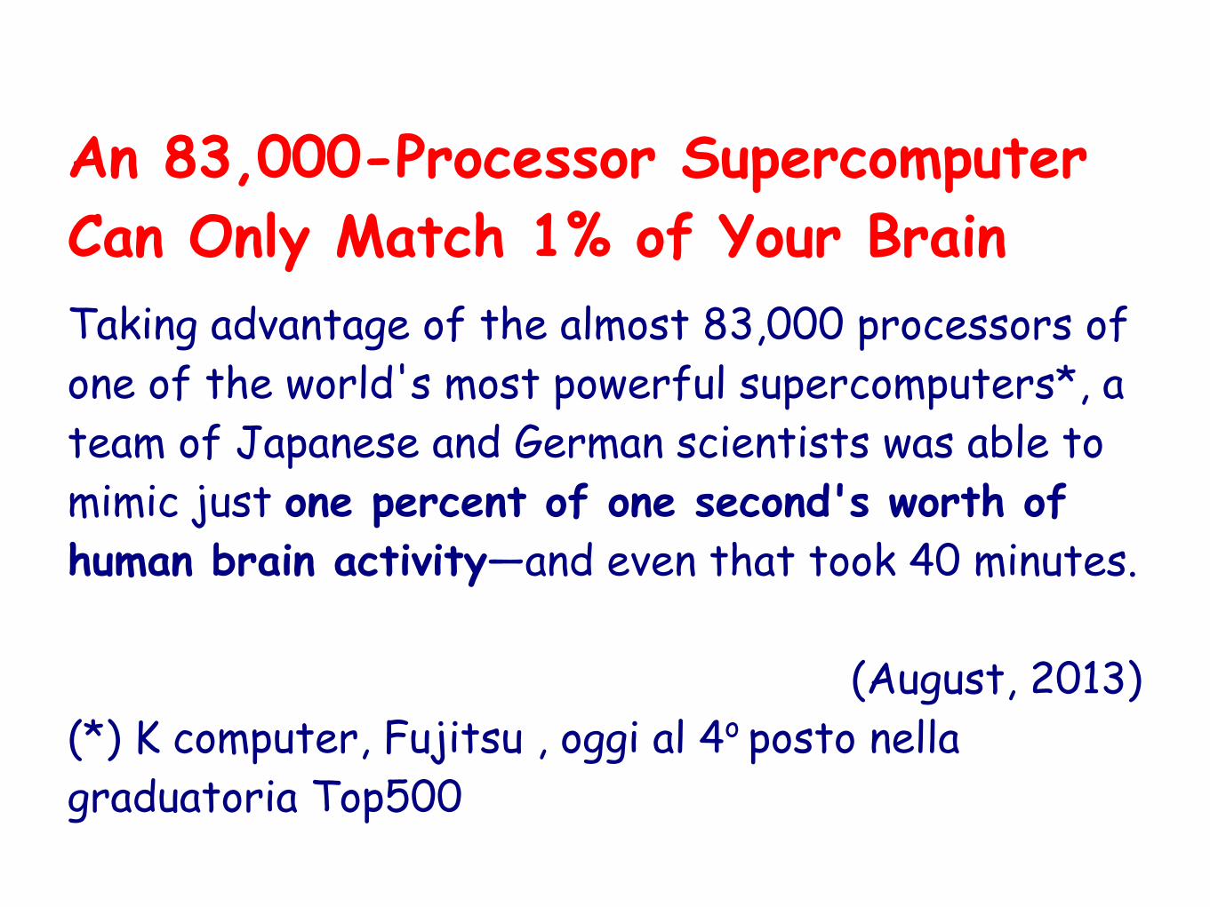
An 83,000-Processor Supercomputer Can Only Match 1% of Your BrainTaking advantage of the almost 83,000 processors of one of the world's most powerful supercomputers*, a team of Japanese and German scientists was able to mimic just one percent of one second's worth of human brain activity—and even that took 40 minutes.

(August, 2013) (*) K computer, Fujitsu , oggi al 4o posto nella graduatoria Top500

che cosa vuol dire per voi questa frase ???che cosa rappresenta per voi il computer e che

uso ne fate???e quale uso pensate di farne in futuro???

The computer is a tool for clear thinking

[Freeman J. Dyson]

domanda per voi!!!

il computer e’ solo un piccolo aiuto...

nella meravigliosa avventura umana

della conoscenza !

The computer is a tool for clear thinking

[Freeman J. Dyson]

interessati a proseguire ancora un po’ in questa

avventura?

http://www.laureescientifiche.units.it/

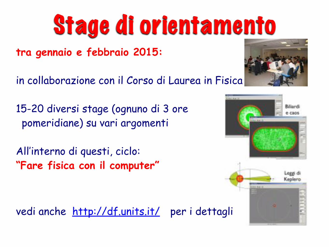
Stage di orientamentotra gennaio e febbraio 2015:

in collaborazione con il Corso di Laurea in Fisica

15-20 diversi stage (ognuno di 3 ore pomeridiane) su vari argomenti

All’interno di questi, ciclo:“Fare fisica con il computer”

vedi anche http://df.units.it/ per i dettagli

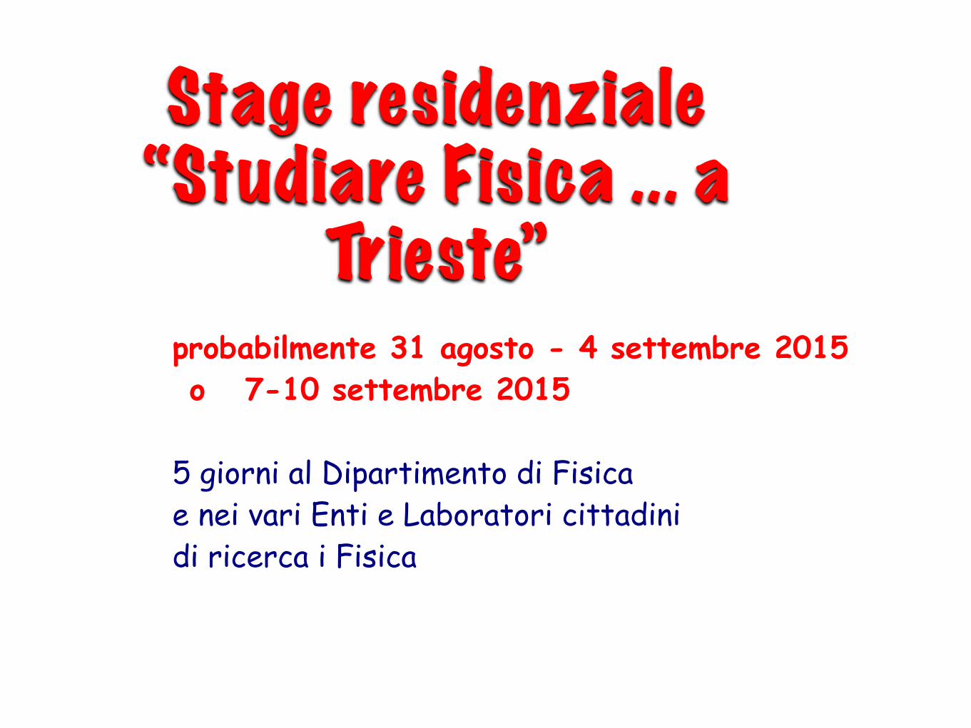
Stage residenziale“Studiare Fisica ... a

Trieste” probabilmente 31 agosto - 4 settembre 2015 o 7-10 settembre 2015

5 giorni al Dipartimento di Fisicae nei vari Enti e Laboratori cittadinidi ricerca i Fisica

...insomma, le occasioni non mancano... di fisica ce n’e’ per tutti i gusti!

... e l’importante e’ sempre saper osservare e stupirsi...

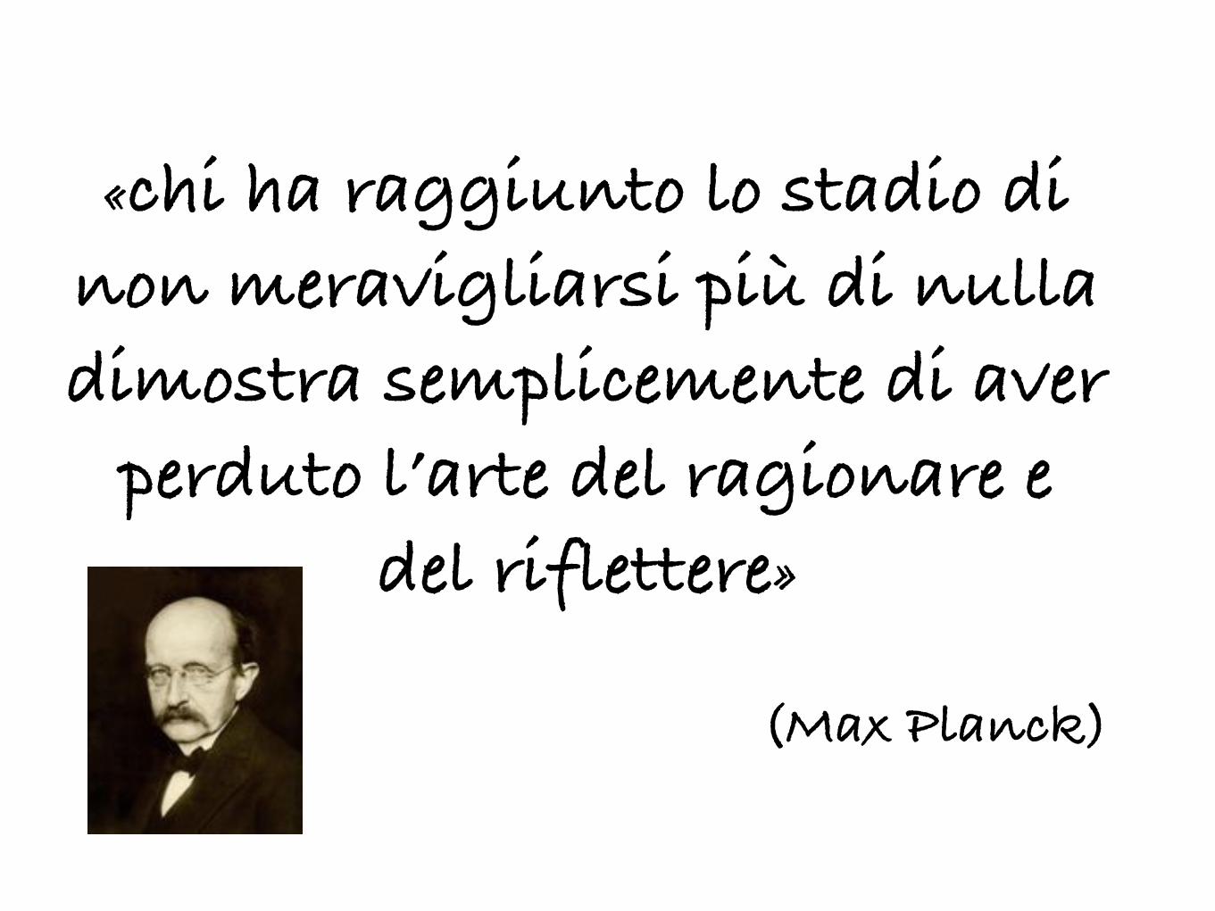
«chi ha raggiunto lo stadio di non meravigliarsi più di nulla dimostra semplicemente di aver

perduto l’arte del ragionare e del riflettere»

(Max Planck)

grazie perl’attenzione!