Fast simulation of stabilizer circuits using a graph-state representation

Fast simulation of stabilizer circuits using a graph-state representation

Simon Anders1,* and Hans J. Briegel1,2

1Institut für Theoretische Physik, Universität Innsbruck, Innsbruck, Austria2Institut für Quantenoptik und Quanteninformation der Österreichischen Akademie der Wissenschaften, Innsbruck, Austria

�Received 25 April 2005; published 21 February 2006�

According to the Gottesman-Knill theorem, a class of quantum circuits—namely, the so-called stabilizercircuits—can be simulated efficiently on a classical computer. We introduce an algorithm for this task, whichis based on the graph-state formalism. It shows significant improvement in comparison to an existing algo-rithm, given by Gottesman and Aaronson, in terms of speed and of the number of qubits the simulator canhandle. We also present an implementation.

DOI: 10.1103/PhysRevA.73.022334 PACS number�s�: 03.67.Lx, 02.70.�c

I. INTRODUCTION

Protocols in quantum-information science often use en-tangled states of a large number of qubits. A major challengein the development of such protocols is to actually test themusing a classical computer. This is because a straight-forwardsimulation is typically exponentially slow and hence intrac-table. Fortunately, the Gottesman-Knill theorem �1,2� statesthat an important subclass of quantum circuits can be simu-lated efficiently: namely, so-called stabilizer circuits. Theseare circuits that use only gates from a restricted subset, theso-called Clifford group. Many techniques in quantum infor-mation use only Clifford gates, most importantly the stan-dard algorithms for entanglement purification �3–7� and forquantum error correction �8–11�. Hence, if one wishes tostudy such networks, one can simulate them numerically.

The usual proof of the Gottesman-Knill theorem �asstated, e.g., in �2�� contains an algorithm that can carry outthis task in time O�N3�, where N is the number of qubits.Especially for the applications just mentioned, one is inter-ested in a large N: For entanglement purification one mightwant to study large ensembles of states and for quantumerror correction concatenations of codes. The cubic scalingrenders this extremely time consuming, and a more efficientalgorithm should be of great use.

Recently, Aaronson and Gottesman presented such an al-gorithm �and an implementation of it called CHP� in Ref.�12�, whose time and space requirements scale only quadrati-cally with the number of qubits. In the present paper, wefurther improve on this by presenting an algorithm that fortypical applications only requires time and space ofO�N log N�. While Aaronson and Gottesman’s simulator,when used on an ordinary desktop computer, can simulatealready systems of several thousands of qubits in a reason-able time, we have used our simulator for over 106 qubits.This provides a valuable tool for investigating complex pro-tocols such as our study of multiparty entanglement purifi-cation protocols in Ref. �13�.

The crucial new ingredient is the use of so-called graphstates. Graph states have been introduced in �14� for the

study of entanglement properties of certain multiqubit sys-tems; they were used as starting point for the one-way quan-tum computer �i.e., measurement-based quantum computing��15� and found to be suited to give a graphical description ofCalderbank-Shor-Steane �CSS� codes �for quantum error cor-rection� �16�. Graph states take their name from the conceptof graphs in mathematics: Each qubit corresponds to a vertexof the graph, and the graph’s edges indicate which qubitshave interacted �see below for details�.

There is an intimate correspondence between stabilizerstates �the class of states that can appear in a stabilizer cir-cuit� and graph states: Not only is every graph state a stabi-lizer state, but also every stabilizer state is equivalent to agraph state in the following sense: Any stabilizer state can betransformed to a graph state by applying a tensor product oflocal Clifford �LC� operations �17–19�. We shall call theselocal Clifford operators the vertex operators �VOp’s�.

To represent a stabilizer state in computer memory, onestores its tableau of stabilizer operators, which is an N�Nmatrix of Pauli operators and hence takes space of orderO�N2� �see below for details�. Gottesman and Aaronson’ssimulator extends this matrix by another matrix of the samesize �which they call the destabilizer tableau�, so that theirsimulator has space complexity O�N2�. A graph state, on theother hand, is described by a mathematical graph, which, forreasons argued later, only needs space of O�N log N� in typi-cal applications. Hence, much larger systems can be repre-sented in memory if one describes them as graph statessupplemented with the list of VOp’s. However, we also needefficient ways to calculate how this representation changes,when the represented state is measured or undergoes aClifford-gate application. The effect of measurements hasbeen extensively studied in �20�, and gate application is whatwe will study in this paper, so that we can then assembleboth to a simulation algorithm.

This paper is organized as follows: We first review thestabilizer formalism, the Gottesman-Knill theorem, and thegraph-state formalism in Sec. II. There, we will also explainour representation in detail. Section III explains how thestate representation changes when Clifford gates are applied.This is the main result and the most technical part of thepaper. For the simulation of measurements, we can rely onthe studies of Ref. �20�, which are reviewed and applied for*Electronic address: [email protected]

PHYSICAL REVIEW A 73, 022334 �2006�

1050-2947/2006/73�2�/022334�9�/$23.00 ©2006 The American Physical Society022334-1

http://dx.doi.org/10.1103/PhysRevA.73.022334

our purpose in Sec. IV. Having exposed all parts of the simu-lator algorithm, we continue by presenting our implementa-tion of it. A reader who only wishes to use our simulator andis not interested in its internal working may want to readonly this section. Section VI assesses the time requirementsof the algorithm’s components described in Secs. III and IVin order to prove our claim of superior scaling of perfor-mance. We finish with a conclusion �Sec. VII�.

II. STABILIZER AND GRAPH STATES

We start by explaining the concepts mentioned in the in-troduction in a formal manner.

Definition 1. The Clifford group CN on N qubits is definedas the normalizer of the Pauli group PN:

CN = �U � SU�2N��UPU† � PN " P � PN� ,

PN = �±1, ± i��I,X,Y,Z��N, �1�

where I is the identity and X, Y, and Z are the usual Paulimatrices.

The Clifford group can be generated by three elementarygates �see, e.g., �2��: the Hadamard gate H, the � /4 phaserotation S, and a two-qubit gate, either the controlled NOT�CNOT� gate �X or the controlled phase gate �Z:

H =1�2

1 1

1 − 1 S = 1 0

0 i ,

�X =�1 0 0 0

0 1 0 0

0 0 0 1

0 0 1 0� �Z =�

1 0 0 0

0 1 0 0

0 0 1 0

0 0 0 − 1� . �2�

The significance of the Clifford group is due to theGottesman-Knill theorem ��1�; see also �2��.

Theorem 1. A quantum circuit using only the followingelements �called a stabilizer circuit� can be simulated effi-ciently on a classical computer: �a� preparation of qubits incomputational basis states, �b� quantum gates from the Clif-ford group, and �iii� measurements in the computational ba-sis.

The proof of the theorem is simple after one introducesthe notion of stabilizer states �21�.

Definition 2. An N-qubit state �� is called a stabilizerstate if it is the unique eigenstate with eigenvalue +1 of Ncommuting multilocal Pauli operators Pa �called the stabi-lizer generators�:

Pa�� = �� , Pa � PN, a = 1,¼,N .

�These N operators generate an Abelian group, the stabilizer,of 2N Pauli operators that all satisfy this stabilization equa-tion.�

Computational basis states are stabilizer states. Further-more, if a Clifford gate U acts on a stabilizer state �� , thenew state U�� is a stabilizer state with generators UPaU†

�PN. Hence, the state in a stabilizer circuit can always be

described by the stabilizer tableau, which is a matrix of N�N operators from �I ,X ,Y ,Z� �where each row is precededby a sign factor�. The effect of an n-qubit gate can then bedetermined by updating nN elements of the matrix, which isan efficient procedure.

Instead of on the stabilizer tableau, we shall base our staterepresentation on graph states.

Definition 3. An N-qubit graph state �G is a quantum stateassociated with a mathematical graph G= �V ,E�, whose �V�=N vertices correspond to the N qubits, while the edges Edescribe quantum correlations, in the sense that �G is theunique state satisfying the N eigenvalue equations

KG�a��G = �G , a � V,

with KG�a� = �x

�a� �b�ngbh a

�z�b�

¬ Xa �b�ngbh a

Zb,

�3�

where ngbh aª �b � �a ,b��E� is the set of vertices adjacentto a �14–16�.

The following theorem states that the edges of the graphcan be associated with phase gate interactions between thecorresponding qubits.

Theorem 2. If one starts with the state �+ �N

=�a�VHa�00¼0 , one can easily construct �G by applying�Z on all pairs of neighboring qubits:

�G = ��a,b��E

�Zab�a�V

Ha�0 �N. �4�

�Proof: insert Eq. �4� into Eq. �3� �20�.�As the operators KG

�a� belong to the Pauli group, all graphstates are stabilizer states, and so are the states which we getby applying local Clifford operators C�C1 to �G . For suchstates, we introduce the notation

�G;C ª �G;C1,C2,¼,CN ª �i=1

N

Ci�G . �5�

It has been shown that all stabilizer states can be broughtinto this form �17–19�; i.e., any stabilizer state is LC equiva-lent to a graph state. �We call two states LC equivalent if onecan be transformed into the other by applying a tensor prod-uct of local Clifford operators.� Finding the graph state thatis LC equivalent to a stabilizer state given by a tableau canbe done by a sort of Gaussian elimination as explained in�17�.

This is what we shall use to represent the current quantumstate in the memory of our simulator. Figure 1 shows for anexample state the tableau representation that is usually em-ployed �and also used by Aaronson and Goldesman’s CHPprogram, albeit in a modified form� and our representation.The tableau representation requires space of order O�N2�. Westore the graph in adjacency list form �i.e., for each vertex, alist of its neighbors is stored�, which needs space of order

O�Nd�, where d is the average vertex degree �number ofneighbors� in the graph. We also store a list of the N localClifford operators C1 ,¼ ,CN, which transform the graphstate �G into the stabilizer state �G ;C . We call these opera-tors the vertex operators. As there are only 24 elements in the

S. ANDERS AND H. J. BRIEGEL PHYSICAL REVIEW A 73, 022334 �2006�

022334-2

local Clifford group, each VOP is represented as a number in0,¼, 23. The scheme to enumerate the 24 operators will bedescribed in �22�. Note that we can disregard global phasesof the VOP’s as they only lead to a global phase of the fullstate of the simulator.

As we shall see later, we may typically assume that d=O�log N�. Hence, our representation needs considerablyless space in memory than a tableau—namely, O�N log N�,including O�N� for the VOP list.

The Gaussian elimination needed to transform a stabilizertableau to its graph-state representation is slow �time com-plexity O�N3��, and so we should better not use it in oursimulator. But usually, one starts with the initial state �0 �N,and if we write this state already in graph-state form, thetableau representation is never used at all.

From Eq. �4�, it is clear that the initial state can be writtenas a graph with no edges and Hadamard gates acting on allvertices:

�0 �N = ��1,¼,N�,��;H,¼,H .

III. GATES

When the simulator is asked to simulate a Clifford gate,the current stabilizer state is changed and its graph represen-tation has to be updated to correctly reflect the action of thegate. How to do this is the main technical result of this paper.

A. Single-qubit gates

In the graph representation, applying local �single-qubit�Clifford gates becomes trivial: if C�C1 is applied to qubit a,we replace this qubit’s VOP Ca by CCa.

B. Two-qubit gates

It is sufficient if the simulator is capable of simulating asingle multi-qubit gate: As the entire Clifford group is gen-erated, e.g., by H, S, and �Z, all gates can be constructed byconcatenating these. We chose to implement �Z, the phasegate, as this is �because of its role in Eq. �4�� most natural forthe graph-state formalism.

In the following discussion, the two qubits onto which thephase gate acts are called the operand vertices and denotedwith a and b. All other qubits are called nonoperand verticesand denoted c, d,¼ .

To solve the task, we have to distinguish several cases.Case 1. The VOP’s of both operand vertices are in Z,

where Zª �I ,Z ,S ,S†� denotes the set of those four localClifford operators that commute with �Z �the other 20 op-erators do not�. In this case, applying the phase gate issimple: We use the fact that �due to Eq. �4�� applying a phasegate on a graph state just toggles an edge:

�Zab��V,E� = ��V,E � ��a,b�� ,

where � denotes the symmetric set difference A�Bª �A�B� \ �A�B�; i.e., the edge �a ,b� is added to the graphif is was not present before; otherwise, it is removed.

FIG. 1. A stabilizer state �� represented indifferent ways: �a� as stabilizer tableau; i.e., thestate is stabilized by the group of Pauli operatorsgenerated by the operators in the four rows. Thisrepresentation needs space O�N2� for N qubits.�b�, �c� as LC equivalence to a graph state. �b�shows the graph, with the VOP’s given by theirdecomposition into the group generators �H ,S�.�c� is the data structure that represents �b� in ouralgorithm. The VOP’s are now specified usingnumbers between 0 and 23 �which enumerate the�C1�=24 LC operators�. Here, we need space

O�Nd�, where d is the average vertex degree—i.e., the average length of the adjacency lists.Writing G for the graph in �b�, we can use thenotation of Eq. �5� and write �� = �G ;H , I ,HS ,S .

FAST SIMULATION OF STABILIZER CIRCUITS¼ PHYSICAL REVIEW A 73, 022334 �2006�

022334-3

Case 2. The VOP of at least one of the operand vertices isnot in Z. In this case, just toggling the edge is not allowedbecause the �Zab cannot be moved past the non-Z VOP. Butthere is a way to change the VOP’s without changing thestate, which works in the following case.

Case 2.2. Both operand vertices have nonoperand neigh-bors. Here, the following operation will help.

Definition 4. The operation of local complementationabout a vertex a of a graph G= �V ,E�, denoted La, is theoperation that inverts the subgraph induced by the neighbor-hood of v:

La�V,E� = �V,E � ��b,c��b,c � ngbh a�� .

This operation transforms the state into a local-Cliffordequivalent one, as the following theorem, taken from�17,20�, asserts.

Theorem 3. Applying the local complementation La onto agraph G yields a state �LaG =U�G , with the multilocal uni-tary

U = �− iXa �b�ngbh a

�iZb � �KG�a�.

Note that the operator �iZ is related to the phase operatorS of Eq. �2�: �iZ=ei�/4S† and

�iX = �− iX† =1�2

1 − i

− i 1 .

An obvious consequence of theorem 3 is the following.Corollary 1. A state �G ;C� is invariant under application

of La to G, followed by an updating of C according to

Cb � �Cb�iX for b = a ,

Cb�− iZ for b � ngbh a ,

Cb otherwise.� �6�

Now note that the local Clifford group is generated notonly by S and H but also by �−iX and �iZ, the Hermitianadjoints of the operators right multiplied by the VOP’s in Eq.�6�. Our simulator has a look-up table that spells out everylocal Clifford operator as a product of—as it turns out, atmost five—of these two operators times a disregarded globalphase. For example, the table’s line for H reads

H � �− iX�iZ�iZ�iZ�− iX . �7�

This allows us now to reduce the VOP Ca of any noniso-lated vertex a to the identity I by proceeding as follows: Thedecomposition of Ca taken from the look-up table is readfrom right to left. When a factor �−iX is read we do a localcomplementation about a. This does not change the state ifthe correction of Eq. �6� is applied, which right-multiplies afactor �iX to Ca. This factor �iX cancels with the factor �−iXat the right-hand end of Ca’s decomposition, so that we nowhave a VOP with a shorter decomposition.

If the rightmost operator of the decomposition is �iZ, wedo a local complementation about an arbitrarily chosenneighbor of a, called a’s “swapping partner.” Now, the cor-rection operation will lead to a factor S being right multipliedby Ca, again shortening the decomposition.

Note that a local complementation about a never changesthe edges incident on a and hence, if a was nonisolated in thebeginning of the procedure, it will stay so. This is important,as only a nonisolated vertex can have a swapping partner.Hence, the procedure can be iterated, and �as the decompo-sitions have a maximum length of 5� after at most five itera-tions, we are left with the identity I as VOP.

We apply the described “VOP reduction procedure” toboth operand vertices. After that, both vertices are the iden-tity, and we can proceed as in case 1.

One might wonder, however, whether the use of the VOPreduction procedure on the second operand vertex b spoilsthe reduction of the VOP of the first operand a. After all, acould be a neighbor of b or of the swapping partner c of b.Then, if a local complementation Lb or Lc is performed, thecompensation according to Eq. �6� changes the neighborhoodof b and c �which include a�. But note that a neighbor of theinversion center only gets a factor �−iZ�S†. As S† generatesZ, this means that after the reduction of b, the VOP of amight be no longer the identity but it is still an element of Z,and we are allowed to go on with case 1.

But what happens if one of the vertices does not have anonoperand neighbor that could serve as swapping partner?This is the next case.

Case 2.2. At least one of the operand vertices is isolatedor only connected to the other operand vertex. We first as-sume that the other vertex is nonconnected in the same sense.

Case 2.2.1. Both operand vertices are either completelyisolated or only connected with each other. Then, we canignore all other vertices and have to study only a finite,rather small number of possible states.

Let us denote by • • the two-vertex graph with no edgesand by •—• the two-vertex graph with one edge. There areonly very few possible two-qubit stabilizer states: namely,those in

S2 ª ��G;C1,C2 �G � �• •,• − •�,C1,C2 � C1� . �8�

Of course, many of the assignments on the right-hand sidedescribe the same state, such that �S2��2�242. Rememberthat the phase gate �Z1,2 �being a Clifford operator� maps S2bijectively onto itself.

The function table of �Z1,2�S2: �G ;C1 ,C2 � �G� ;C1� ,C2�

can easily be computed in advance �we did it with Math-ematica� and hard coded into the simulator as a look-uptable. This table contains 2�242 lines such as

�• •,C�13�,C�2� � �• − •,C�0�,C�2� , �9�

where the C�i��i=0,¼ ,23� are the Clifford operators in theenumeration detailed in �22� �e.g., C�0�= I, C�2�=Y�.

Note that many of the assignments to C1 and C2 in Eq. �8�describe the same state. Hence, we have a choice in the op-erators C1�, C2� with which we represent the results of thephase gate in the look-up table. It turns out �by inspection ofall the possibilities� that we can always choose the operatorssuch that the following constraint is fulfilled.

Constraint 1. If C1�C2��Z, choose C1�, C2� such thatagain C1��C2��Z.

The use of this will become clear soon.


022334-4

Case 2.2.2. We are left with one last case—namely, thatone vertex, let it be a, is connected with nonoperand neigh-bors, but the other vertex b is not—i.e., has either no neigh-bors or only a as neighbor. Then, we proceed as follows: Weuse iterated local complementations to reduce Ca to I. After

that, we may use the look-up table as in case 2.2.1. That thisis allowed even though a is connected to a nonoperand ver-tex is shown in the following: First note that the state afterthe reduction of Ca to I can be written �following Eq. �5��as

�where =0,1 indicates whether �a ,b��E�. Observe that Cb

has been moved past the operators �Zcd. This is allowedbecause none of the �Zcd acts on b.

We now apply �Zab to this state. �Zab can be movedthrough all the phase gates and vertex operators above theleft brace so that it stands right in front of the S2 state �� ab

which is separated from the rest. Thus, the table �9� fromcase 2.2.1 may be used. �This would not be the case if, in thestate above the brace marked with �*�, the two operand ver-tices were still entangled with other qubits.� The look-up inthe table will give new operators Ca�, Cb� and a new �, so thatthe new state has the following form:

�Zab��V,E�;C = �c�V\�a,b�

Cc ��c,d��E\��a,b��

�Zcd

�Ca�Cb��Zab�� + + ¯ + . �10�

For this to be a state in our usual �G ;C form �5�, the twooperators Ca� and Cb� have to moved to the left, through the�Zcd. For Cb�, this is no problem, as b was assumed to beeither isolated or connected only to a, so that Cb� commuteswith ��c,d��E\��a,b��Zcd, as the latter operator does not act onb. The vertex a, however, has connections to nonoperandneighbors, so that some of the �Zcd act on it. We may moveit only if Ca��Z �as this means that it commutes with �Z�.Luckily, due to constraint 1 imposed above, we can be surethat Ca��Z, because Ca= I�Z.

Figure 2 shows as listing in pseudocode how these resultscan be used to actually implement the controlled phase gate�Z.

IV. MEASUREMENTS

In a stabilizer circuit, the simulator may be asked at anypoint to simulate the measurement of a qubit in the compu-tational basis. How the outcome of the measurement is de-termined and how the graph representation has to be updatedin order to then represent the post-measurement state will beexplained in the following.

To measure a qubit a of a state �G ,C in the computa-tional basis means to measure the qubit in the underlyinggraph state �G in one of the three Pauli bases. Writing themeasurement outcome as , this means

I + �− 1�Za

2�G,C = �

b�V\�a�Cb I + �− 1�Za

2Ca�G

= �b�V\�a�

CbCa

I + �− 1�Ca†ZaCa

2�G .

�11�

As Ca is a Clifford operator, PaªCa†ZaCa� �Xa ,Ya ,Za ,

−Xa ,−Ya ,−Za�. Thus, in order to measure qubit a of �G ,C inthe computational basis, we measure the observable Pa on�G . Note that in case that Pa is the negative of a Paulioperator, the measurement result to be reported by thesimulator is the complement of , the result given by the X,Y, or Z measurement on the underlying graph state �G .

How is the graph G changed and how do the vertex op-erators have to be modified if the measurement��I± Pa� /2��G is carried out? This has been worked out indetail in Ref. �20�, which we now briefly review for thepresent purpose.

The simplest case is that of P= ±Z. Here, the statechanges as follows:

�12�


022334-5

The value of is chosen at random �using a pseudo-random-number generator�. To update the simulator state, the VOP’sare right multiplied by the underbraced operators �*� and theedges incident on a are deleted as indicated in the ket.

A measurement of the Y observable �P= ±Y� requires acomplementation of the edges set according to

E � E � ��b,c��b,c � ngbha�

and a change in the VOP’s as follows:

Cb � Cb�− iZ�†� for b � ngbha � �a� ,

where the dagger in parentheses is to be read only for mea-

surement result =1.The most complicated case is the X measurement which

requires an update of edges and VOP’s as follows:

E � E � ��c,d��c � ngbhb,d � ngbha�

� ��c,d��c,d � ngbhb � ngbha�

� ��b,d��d � ngbha \ �b�� ,

Cc ��CcZ

for c = a ,

Cc�iY�†� for c = b �read ‘‘ † ’’ only for = 1� ,

CcZ for c � �ngbh a \ ngbh b \ �b�

�for = 0� ,

ngbh b \ ngbh a \ �a�

�for = 1� ,�

Cc otherwise.

��13�

Here, b is a vertex chosen arbitrarily from ngbh a and

�iY =1�2

1 − 1

1 1 .

In all these cases the measurement result is chosen atrandom. Only in the case of the measurement of Pa= ±X an

isolated vertexis the result always =0 �which means an ac-tual result of =0 for Pa=X and =1 for Pa=−X�.

V. IMPLEMENTATION

The algorithm described above has been implemented inC�� in object-oriented programming style. We have usedthe GNU Compiler Collection �GCC� �24� under Linux, butit should be easy to compile the program on other platformsas well �28�. The implementation is done as a library to allowfor easy integration into other projects. We also offer bind-ings to PYTHON �25�, so that the library can be used by PY-

THON programs as well. �This was achieved using SWIG

�26�.�The simulator, called “GRAPHSIM,” can be downloaded

from �23�.A detailed documentation of the library is supplied with it.

To demonstrate the usage here at least briefly, we give Fig. 3

FIG. 2. Pseudocode for controlled phase gate ��Z� acting onvertices a and b �“cphase”� and for the two auxiliary routines “re-move VOP” and “local complementation”.


022334-6

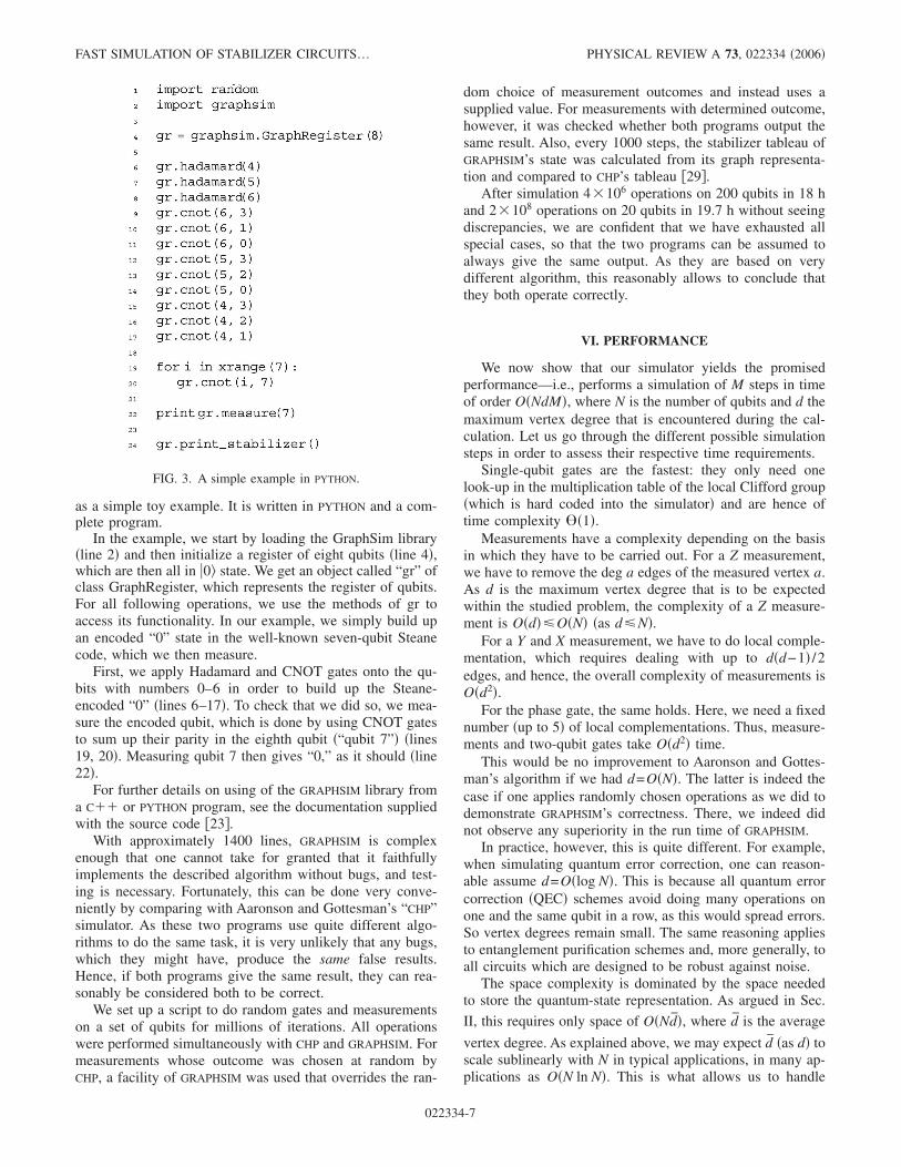
as a simple toy example. It is written in PYTHON and a com-plete program.

In the example, we start by loading the GraphSim library�line 2� and then initialize a register of eight qubits �line 4�,which are then all in �0 state. We get an object called “gr” ofclass GraphRegister, which represents the register of qubits.For all following operations, we use the methods of gr toaccess its functionality. In our example, we simply build upan encoded “0” state in the well-known seven-qubit Steanecode, which we then measure.

First, we apply Hadamard and CNOT gates onto the qu-bits with numbers 0–6 in order to build up the Steane-encoded “0” �lines 6–17�. To check that we did so, we mea-sure the encoded qubit, which is done by using CNOT gatesto sum up their parity in the eighth qubit �“qubit 7”� �lines19, 20�. Measuring qubit 7 then gives “0,” as it should �line22�.

For further details on using of the GRAPHSIM library froma C�� or PYTHON program, see the documentation suppliedwith the source code �23�.

With approximately 1400 lines, GRAPHSIM is complexenough that one cannot take for granted that it faithfullyimplements the described algorithm without bugs, and test-ing is necessary. Fortunately, this can be done very conve-niently by comparing with Aaronson and Gottesman’s “CHP”simulator. As these two programs use quite different algo-rithms to do the same task, it is very unlikely that any bugs,which they might have, produce the same false results.Hence, if both programs give the same result, they can rea-sonably be considered both to be correct.

We set up a script to do random gates and measurementson a set of qubits for millions of iterations. All operationswere performed simultaneously with CHP and GRAPHSIM. Formeasurements whose outcome was chosen at random byCHP, a facility of GRAPHSIM was used that overrides the ran-

dom choice of measurement outcomes and instead uses asupplied value. For measurements with determined outcome,however, it was checked whether both programs output thesame result. Also, every 1000 steps, the stabilizer tableau ofGRAPHSIM’s state was calculated from its graph representa-tion and compared to CHP’s tableau �29�.

After simulation 4�106 operations on 200 qubits in 18 hand 2�108 operations on 20 qubits in 19.7 h without seeingdiscrepancies, we are confident that we have exhausted allspecial cases, so that the two programs can be assumed toalways give the same output. As they are based on verydifferent algorithm, this reasonably allows to conclude thatthey both operate correctly.

VI. PERFORMANCE

We now show that our simulator yields the promisedperformance—i.e., performs a simulation of M steps in timeof order O�NdM�, where N is the number of qubits and d themaximum vertex degree that is encountered during the cal-culation. Let us go through the different possible simulationsteps in order to assess their respective time requirements.

Single-qubit gates are the fastest: they only need onelook-up in the multiplication table of the local Clifford group�which is hard coded into the simulator� and are hence oftime complexity �1�.

Measurements have a complexity depending on the basisin which they have to be carried out. For a Z measurement,we have to remove the deg a edges of the measured vertex a.As d is the maximum vertex degree that is to be expectedwithin the studied problem, the complexity of a Z measure-ment is O�d��O�N� �as d�N�.

For a Y and X measurement, we have to do local comple-mentation, which requires dealing with up to d�d−1� /2edges, and hence, the overall complexity of measurements isO�d2�.

For the phase gate, the same holds. Here, we need a fixednumber �up to 5� of local complementations. Thus, measure-ments and two-qubit gates take O�d2� time.

This would be no improvement to Aaronson and Gottes-man’s algorithm if we had d=O�N�. The latter is indeed thecase if one applies randomly chosen operations as we did todemonstrate GRAPHSIM’s correctness. There, we indeed didnot observe any superiority in the run time of GRAPHSIM.

In practice, however, this is quite different. For example,when simulating quantum error correction, one can reason-able assume d=O�log N�. This is because all quantum errorcorrection �QEC� schemes avoid doing many operations onone and the same qubit in a row, as this would spread errors.So vertex degrees remain small. The same reasoning appliesto entanglement purification schemes and, more generally, toall circuits which are designed to be robust against noise.

The space complexity is dominated by the space neededto store the quantum-state representation. As argued in Sec.

II, this requires only space of O�Nd�, where d is the average

vertex degree. As explained above, we may expect d �as d� toscale sublinearly with N in typical applications, in many ap-plications as O�N ln N�. This is what allows us to handle

FIG. 3. A simple example in PYTHON.


022334-7

substantially more qubits than is possible with the O�N2�tableau representation.

As a first practical test, we used GRAPHSIM to simulateentanglement purification of cluster states with the protocolof Ref. �7�. This has been a starting point of a detailed analy-sis of the communication costs of establishing multipartiteentanglement states via noisy channels �13�. Figure 4 dem-onstrates that GRAPHSIM is indeed suitable for this purpose.Note that for the rightmost data points, the register holds30 000 qubits.

As we did a Monte Carlo simulation, we had to loop thecalculation very often and still got an output within a fewhours. For simulations involving several millions of qubitsand a large number of runs, we waited about a week for theresults when using eight processors in parallel. We redidsome of these calculations in a more controlled testing envi-ronment as a benchmark for GRAPHSIM. Figure 5 shows theresults in a log-log plot.

VII. CONCLUSION

To summarize, we have used recent results on graph statesto find a very space-efficient representation of stabilizer

states and determined how this representation changes underthe action of Clifford gates. This can be used to simulatestabilizer circuits more efficiently than previously possible.The gain is not only in simulation speed, but also in thenumber of manageable qubits. In the latter, at least two or-ders of magnitude are gained. We have presented an imple-mentation of our simulation algorithm and will soon publishresults about entanglement purification which makes use ofour technique.

ACKNOWLEDGMENTS

We would like to thank Marc Hein for most helpful dis-cussions. This work was supported in part by the AustrianScience Foundation �FWF�, the Deutsche Forschungsge-meinschaft �DFG�, and the European Union �Grant Nos. IST-2001-38877 and IST-2001-39227, OLAQUI, SCALA�.

�1� D. Gottesman, e-print quant-ph/9807006.�2� M. A. Nielsen and I. L. Chuang, Quantum Computation and

Quantum Information �Cambridge University Press, Cam-bridge, England, 2000�.

�3� C. H. Bennett, G. Brassard, S. Popescu, B. Schumacher, J. A.Smolin, and W. K. Wootters, Phys. Rev. Lett. 76, 722 �1996�.

�4� D. Deutsch, A. Ekert, R. Jozsa, C. Macchiavello, S. Popescu,and A. Sanpera, Phys. Rev. Lett. 77, 2818 �1996�.

�5� M. Murao, M. B. Plenio, S. Popescu, V. Vedral, and P. L.Knight, Phys. Rev. A 57, R4075 �1998�.

�6� E. N. Maneva and J. A. Smolin, in Quantum Computation andQuantum Information, edited by J. S. J. Lomonaco �AMS,Providence, RI, 2002�; also e-print quant-ph/0003099.

�7� W. Dür, H. Aschauer, and H. J. Briegel, Phys. Rev. Lett. 91,107903 �2003�.

�8� P. W. Shor, Phys. Rev. A 52, R2493 �1995�.�9� A. M. Steane, Phys. Rev. Lett. 77, 793 �1996�.

�10� A. R. Calderbank and P. W. Shor, Phys. Rev. A 54, 1098�1996�.

�11� A. M. Steane, Proc. R. Soc. London, Ser. A 452, 2551 �1996�.�12� S. Aaronson and D. Gottesman, Phys. Rev. A 70, 052328

�2004�.�13� C. Kruszynska, S. Anders, W. Dür, and H. J. Briegel, e-print

quant-ph/0512218�14� H. J. Briegel and R. Raußendorf, Phys. Rev. Lett. 86, 910

�2001�.

FIG. 4. Comparison of the performance of CHP and GRAPHSIM. Asimulation of entanglement purification was used as sample appli-cation. The register has 1000 times the size of the states to hold anensemble of 1000 states.

FIG. 5. Benchmark of GRAPHSIM for very large registers. En-tanglement purification—specifically, the purification of ten-qubitcluster states with the protocol of Ref. �7�—was used as sampleproblem. The register was filled up with cluster states to make alarge ensemble, and two protocol steps were simulated. The averagetime per operation was obtained from the total run time �27�.


022334-8

�15� R. Raußendorf, D. E. Browne, and H. J. Briegel, Phys. Rev. A68, 022312 �2003�.

�16� D. Schlingemann and R. F. Werner, Phys. Rev. A 65, 012308�2002�.

�17� M. Van den Nest, J. Dehaene, and B. De Moor, Phys. Rev. A69, 022316 �2004�.

�18� M. Grassl, A. Klappenecker, and M. Rötteler, in Proceedingsof the 2002 IEEE International Symposium on InformationTheory, �IEEE, New York, 2002�, p. 45.

�19� D. Schlingemann, e-print quant-ph/0111080.�20� M. Hein, J. Eisert, and H. J. Briegel, Phys. Rev. A 69, 062311

�2004�.�21� D. Gottesman, Ph.D. thesis, California Institute of Technology,

1997, e-print quant-ph/9705052.�22� S. Anders �unpublished�.�23� The described software can be found at http://

homepage.uibk.ac.at/homepage/c705/c705213/work/graphsim.html

�24� The GCC Team, The GNU Compiler Collection, software athttp://gcc.gnu.org

�25� PYTHON, programming language developped by Guido vanRossum et al., http://www.python.org

�26� SWIG (simplified wrapper and interface generator), softwaredeveloped by David M. Beazley et al., http://www.swig.org

�27� Giving the time per operation in seconds is of use only whenone specifies the machine which has run the code: We usedLinux computers with AMD Opteron processors, clocked with2.2 GHz. Only one the machine’s several processors was dedi-cated to our computation task. The code was compiled usingthe GNU C�� compiler �version 3.2.3� with 64-bit target and“O3” optimization.

�28� We use only ISO Standard C�� with one exception: The hashset template is used, which is, though, not part of the standard,supplied by most modern compilers.

�29� This was done with a Mathematica subroutine which tries tofind a row adding and swapping arrangement to transform onetableau into the other.


022334-9

Documents

Fast simulation of stabilizer circuits using a graph-state representation